Static Games of Complete Information: Subgame Perfection

APEC 8205: Applied Game Theory

Objectives

• Why is Nash not enough in dynamic games of complete information?

• Subgame Perfect Refinement to Nash Equilibrium– What is a subgame?

– Definition of Subgame Perfect Equilibrium

– Application of Subgame Perfect Equilibrium• Stackelberg Duopoly

• Stackelberg Rent Seeking

– Empirical Weaknesses of Subgame Perfection

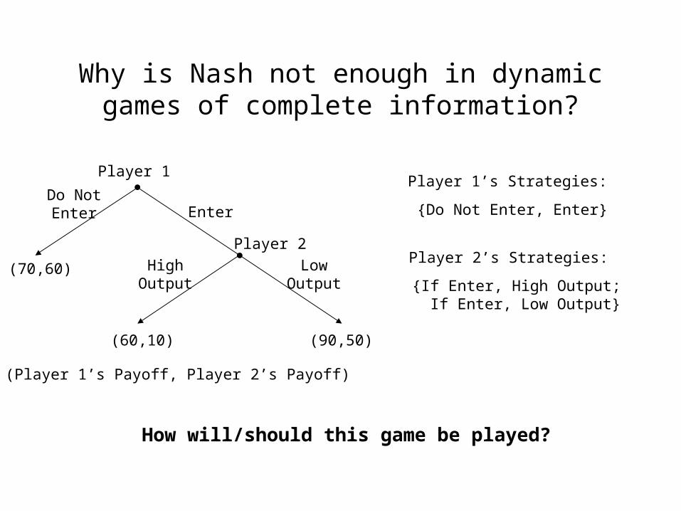
Why is Nash not enough in dynamic games of complete information?

Player 1

EnterDo NotEnter

(70,60)

(Player 1’s Payoff, Player 2’s Payoff)

Player 2

HighOutput

LowOutput

(60,10) (90,50)

Player 1’s Strategies:

{Do Not Enter, Enter}

Player 2’s Strategies:

{If Enter, High Output; If Enter, Low Output}

How will/should this game be played?

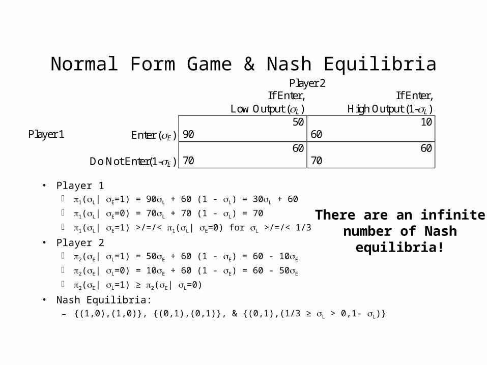
Normal Form Game & Nash Equilibria

• Player 1 1(L| E=1) = 90L + 60 (1 - L) = 30L + 60

1(L| E=0) = 70L + 70 (1 - L) = 70

1(L| E=1) >/=/< 1(L| E=0) for L >/=/< 1/3

• Player 2 2(E| L=1) = 50E + 60 (1 - E) = 60 - 10E

2(E| L=0) = 10E + 60 (1 - E) = 60 - 50E

2(E| L=1) ≥ 2(E| L=0)

• Nash Equilibria: – {(1,0),(1,0)}, {(0,1),(0,1)}, & {(0,1),(1/3 ≥ L > 0,1- L)}

Player 2 If Enter,

Low Output (L) If Enter,

High Output (1-L)

Player 1

Enter (E) 50

90 10

60

Do Not Enter(1-E) 60

70 60

70

There are an infinitenumber of Nash

equilibria!

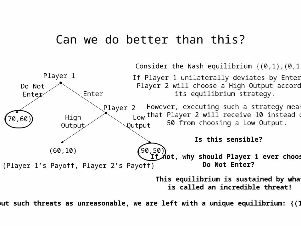
Can we do better than this?

Player 1

EnterDo NotEnter

(70,60)

(Player 1’s Payoff, Player 2’s Payoff)

Player 2

HighOutput

LowOutput

(60,10) (90,50)

Consider the Nash equilibrium {(0,1),(0,1)}!

If Player 1 unilaterally deviates by Entering,Player 2 will choose a High Output according

its equilibrium strategy.

However, executing such a strategy meansthat Player 2 will receive 10 instead of

50 from choosing a Low Output.

Is this sensible?

If not, why should Player 1 ever chooseDo Not Enter?

This equilibrium is sustained by whatis called an incredible threat!

If we rule out such threats as unreasonable, we are left with a unique equilibrium: {(1,0),(1,0)}!

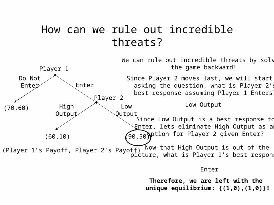
How can we rule out incredible threats?

Player 1

EnterDo NotEnter

(70,60)

(Player 1’s Payoff, Player 2’s Payoff)

Player 2

HighOutput

LowOutput

(60,10) (90,50)

We can rule out incredible threats by solvingthe game backward!

Since Player 2 moves last, we will start byasking the question, what is Player 2’s

best response assuming Player 1 Enters?

Low Output

Since Low Output is a best response toEnter, lets eliminate High Output as an

option for Player 2 given Enter?

Now that High Output is out of thepicture, what is Player 1’s best response?

Enter

Therefore, we are left with the unique equilibrium: {(1,0),(1,0)}!

Subgame Definition

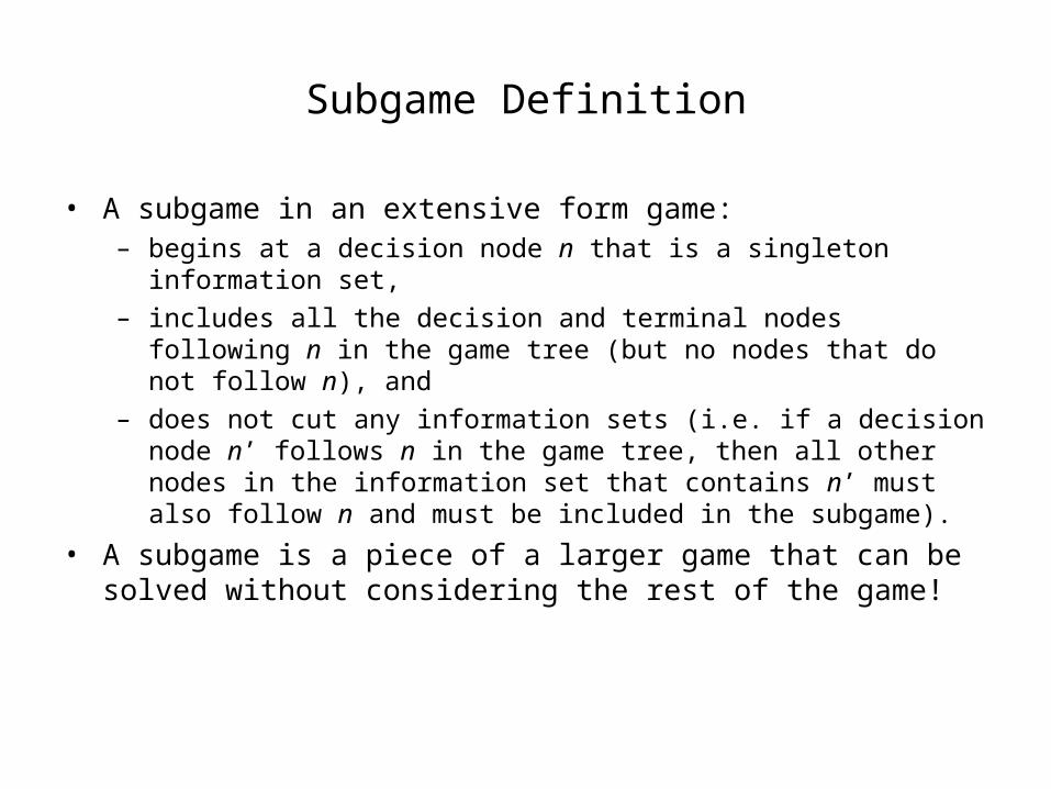
• A subgame in an extensive form game:– begins at a decision node n that is a singleton information set,

– includes all the decision and terminal nodes following n in the game tree (but no nodes that do not follow n), and

– does not cut any information sets (i.e. if a decision node n’ follows n in the game tree, then all other nodes in the information set that contains n’ must also follow n and must be included in the subgame).

• A subgame is a piece of a larger game that can be solved without considering the rest of the game!

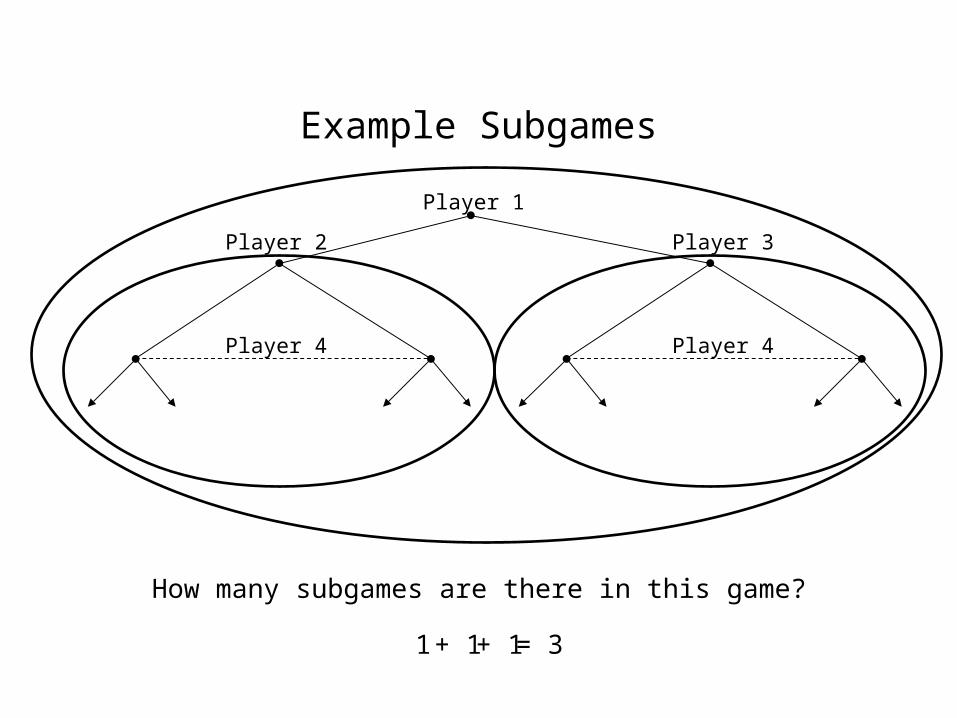
Example Subgames

Player 1

Player 2 Player 3

Player 4 Player 4

How many subgames are there in this game?

1 + 1 + 1 = 3

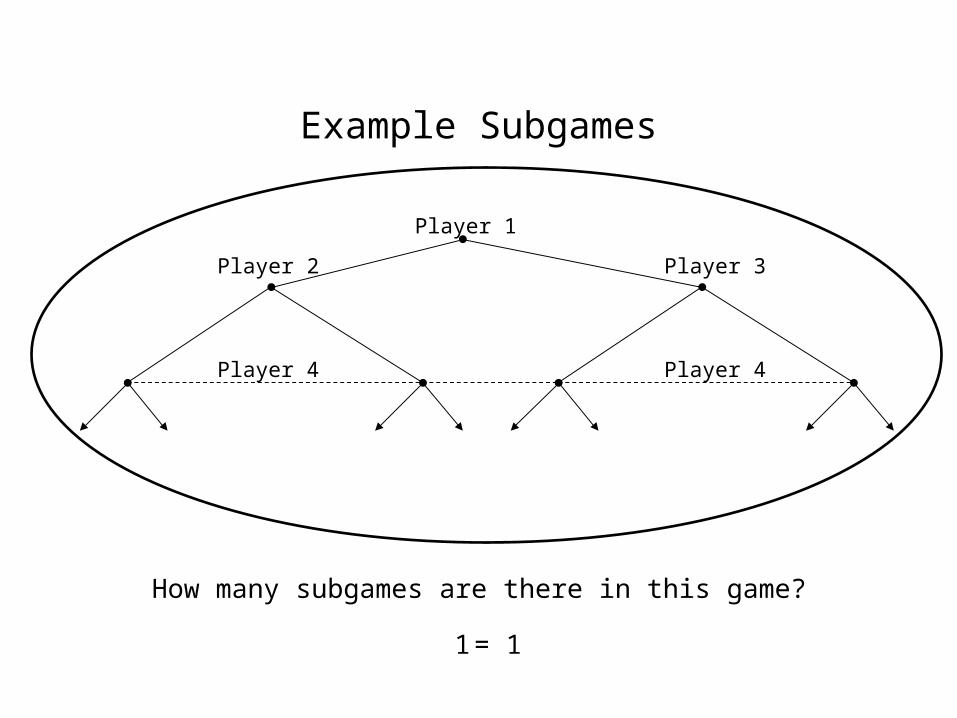
Example Subgames

Player 1

Player 2 Player 3

Player 4 Player 4

How many subgames are there in this game?

1 = 1

Subgame Perfect Equilibrium

• A Nash equilibrium is subgame perfect if the players’ strategies constitute a Nash equilibrium in every subgame (Selten, 1965).

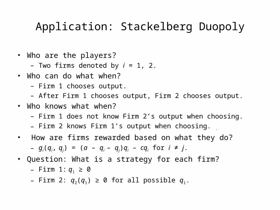
Application: Stackelberg Duopoly

• Who are the players?– Two firms denoted by i = 1, 2.

• Who can do what when? – Firm 1 chooses output.

– After Firm 1 chooses output, Firm 2 chooses output.

• Who knows what when?– Firm 1 does not know Firm 2’s output when choosing.

– Firm 2 knows Firm 1’s output when choosing. .

• How are firms rewarded based on what they do?– gi(qi, qj) = (a – qi – qj)qi – cqi for i ≠ j.

• Question: What is a strategy for each firm?– Firm 1: q1 ≥ 0

– Firm 2: q2(q1) ≥ 0 for all possible q1.

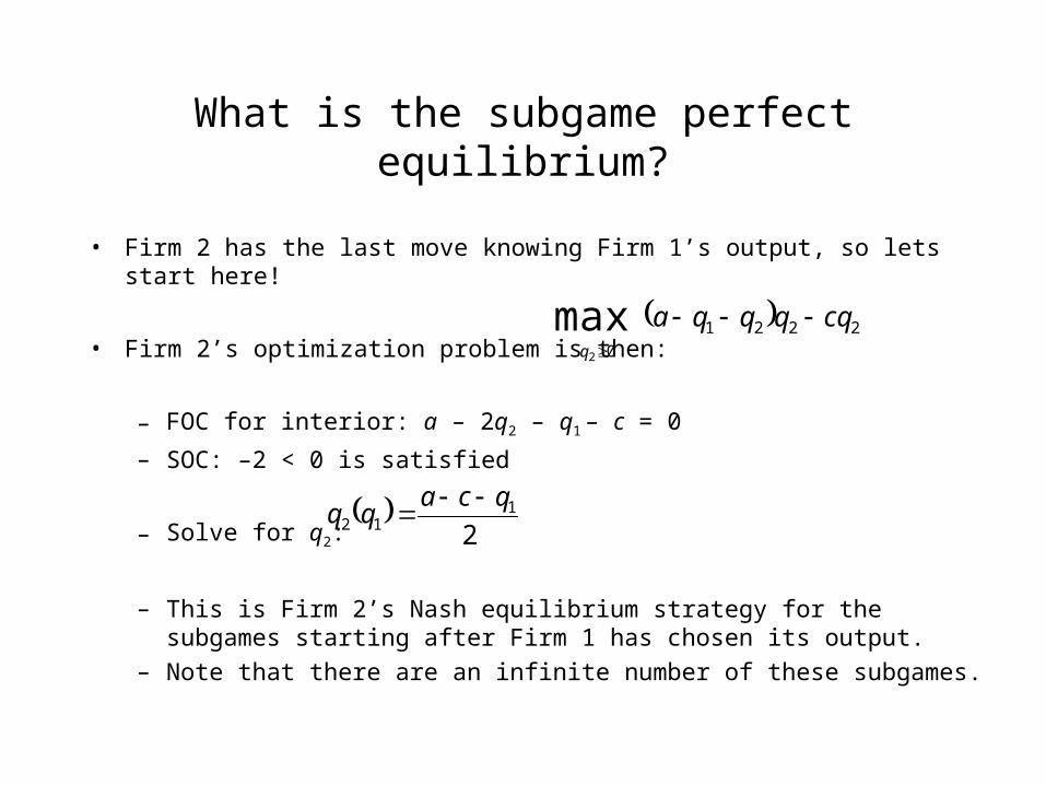
What is the subgame perfect equilibrium?

• Firm 2 has the last move knowing Firm 1’s output, so lets start here!

• Firm 2’s optimization problem is then:

– FOC for interior: a – 2q2 – q1 – c = 0

– SOC: –2 < 0 is satisfied

– Solve for q2:

– This is Firm 2’s Nash equilibrium strategy for the subgames starting after Firm 1 has chosen its output.

– Note that there are an infinite number of these subgames.

2221

0

max2

cqqqqaq

2

112

qcaqq

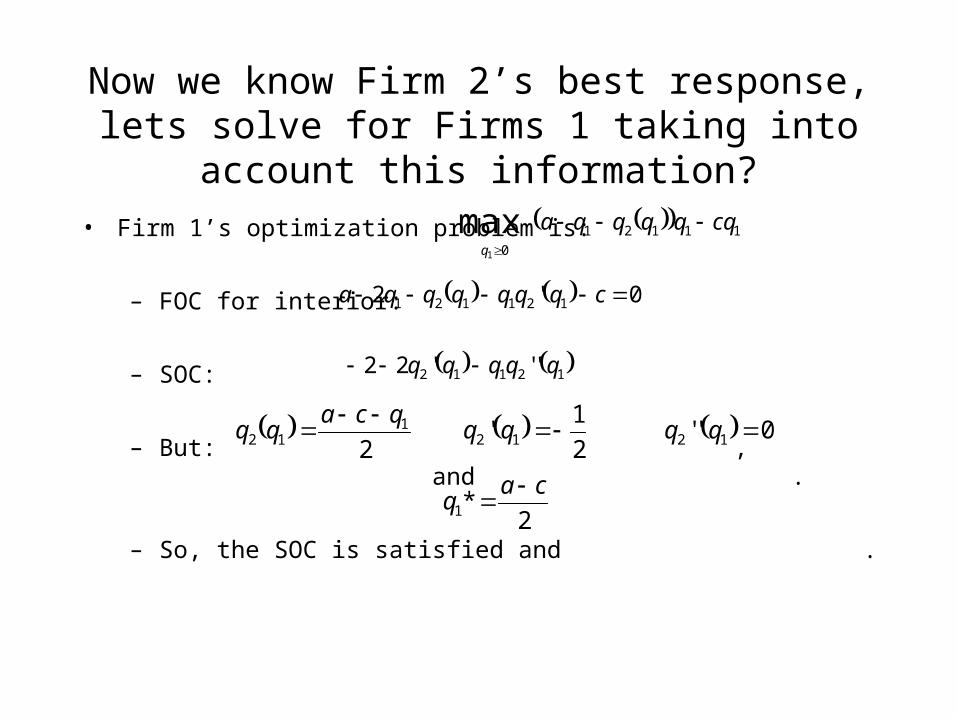
Now we know Firm 2’s best response, lets solve for Firms 1 taking into account this information?

• Firm 1’s optimization problem is:

– FOC for interior:

– SOC:

– But: , and .

– So, the SOC is satisfied and .

11121

0

max1

cqqqqqaq

2

112

qcaqq

0'2 121121 cqqqqqqa

12112 '''22 qqqqq

2

1' 12 qq 0'' 12 qq

2*1

caq

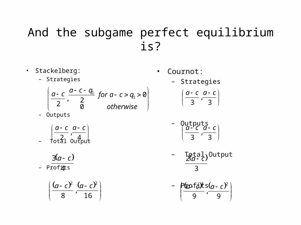
And the subgame perfect equilibrium is?

• Stackelberg:– Strategies

– Outputs

– Total Output

– Profits

• Cournot:– Strategies

– Outputs

– Total Output

– Profits

otherwise

qcaforqcaca

0

02,

21

1

3,

3

caca

4,

2

caca

4

3 ca

3,

3

caca

3

2 ca

9

,9

22 caca

16

,8

22 caca

Implications Regarding the Impacts of Better Information for Firm 2

• Output– Firm 1’s Increases

– Firm 2’s Decreases

– Total Increases

• Profit– Firm 1’s Increases

– Firm 2’s Decreases

– Total Profit Decreases

Even though Firm 2 has better information to make its choice, it is worse off!

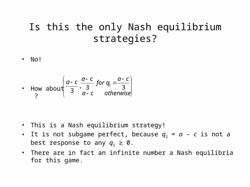
Is this the only Nash equilibrium strategies?

• No!

• How about ?

• This is a Nash equilibrium strategy!

• It is not subgame perfect, because q2 = a – c is not a best response to any q1 ≥ 0.

• There are in fact an infinite number a Nash equilibria for this game.

otherwiseca

caqfor

caca33,

31

Application: Stackelberg Rent Seeking

• Who are the players?– Two firms denoted by i = 1, 2 competing for a lucrative contract worth Vi.

• Who can do what when? – Firm 1 chooses effort (x1) for preparing its proposal.

– After Firm 1 chooses effort, Firm 2 chooses effort (x2).

• Who knows what when?– Firm 1 does not know Firm 2’s effort when choosing.

– Firm 2 knows Firm 1’s effort when choosing. .

• How are firms rewarded based on what they do?– gi(xi, xj) = Vi xi / (xj + xj) – xi for i ≠ j.

• Question: What is a strategy for each firm?– Firm 1: x1 ≥ 0

– Firm 2: x2(x1) ≥ 0 for all possible x1.

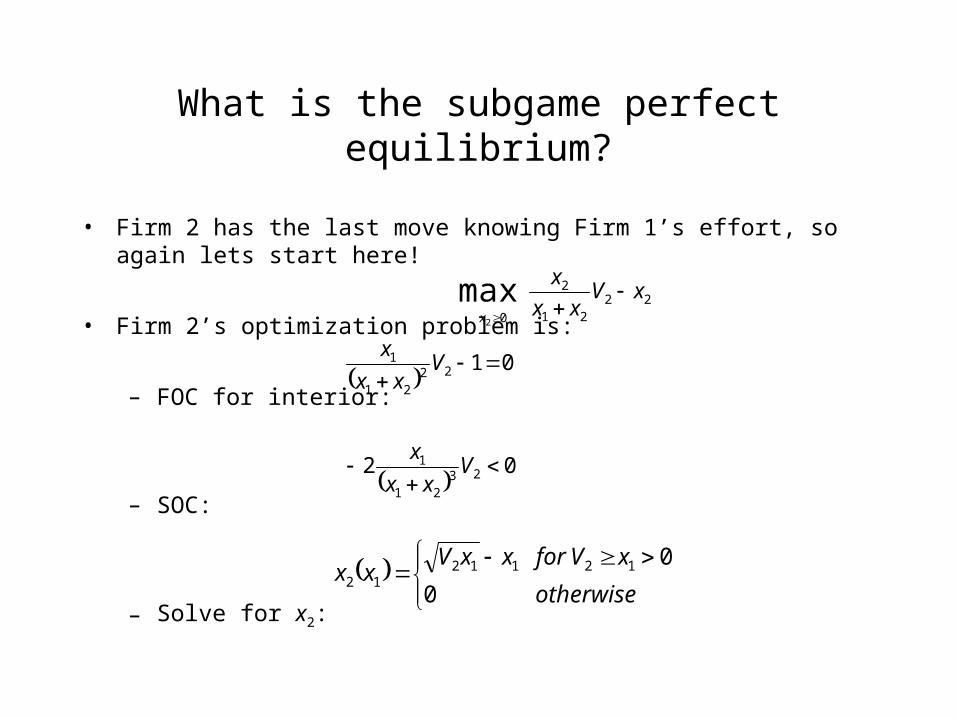
What is the subgame perfect equilibrium?

• Firm 2 has the last move knowing Firm 1’s effort, so again lets start here!

• Firm 2’s optimization problem is:

– FOC for interior:

– SOC:

– Solve for x2:

2221

2

0

max2

xVxx

x

x

otherwise

xVforxxVxx

0

01211212

0122

21

1

Vxx

x

02 23

21

1

Vxx

x

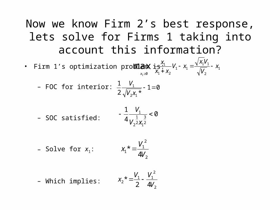
Now we know Firm 2’s best response, lets solve for Firms 1 taking into account this information?

• Firm 1’s optimization problem is:

– FOC for interior:

– SOC satisfied:

– Solve for x1:

– Which implies:

1

2

1111

21

1

0

max1

xV

VxxV

xx

x

x

01*2

1

12

1 xV

V

04

1

2

3

12

1

2

1 xV

V

2

21

1 4*

V

Vx

2

211

2 42*

V

VVx

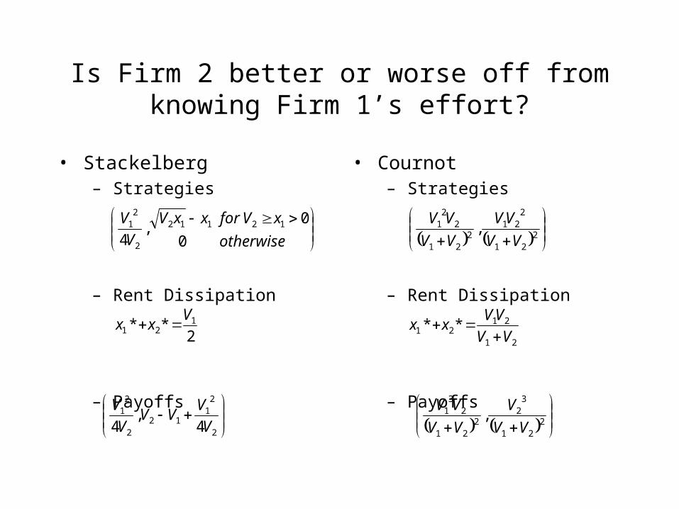
Is Firm 2 better or worse off from knowing Firm 1’s effort?

• Stackelberg– Strategies

– Rent Dissipation

– Payoffs

• Cournot– Strategies

– Rent Dissipation

– Payoffs

otherwise

xVforxxV

V

V

0

0,

412112

2

21

221

221

221

22

1 ,VV

VV

VV

VV

2

21

122

21

4,

4 V

VVV

V

V

221

32

221

23

1 ,VV

V

VV

VV

2** 1

21

Vxx

21

2121 **

VV

VVxx

Implications

• Firm 1 better off with Firm 2 knowing its effort.

• Firm 2 may be better or worse off knowing Firm 1’s effort:– Better off if V2 > V1 > 0

– Worse off if 2V2 > V1 > V2

• So we can get results contrary to the duopoly model. Having more information is not always bad!

• Why?– Information Effect: Beneficial to Second Mover

– Timing Effect: Detrimental to Second Mover

• In the Duopoly model with linear demand the timing effect always dominates.

• In the Rent Seeking model, the information effect can dominate.

Predictive Weaknesses of Subgame Perfection

• Incredible Threats That Are Actually Credible

• Pareto Improving Non-Equilibrium Play

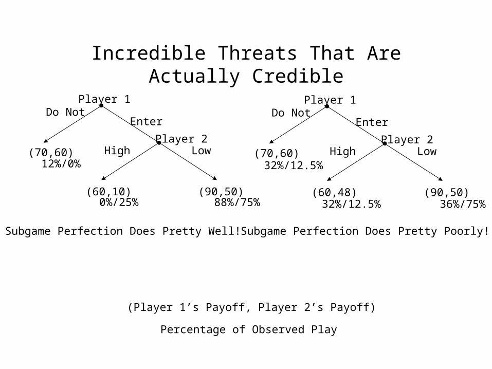
Incredible Threats That Are Actually Credible

(Player 1’s Payoff, Player 2’s Payoff)

Player 1

EnterDo Not

(70,60)Player 2

High Low

(60,10) (90,50)

12%/0%

0%/25% 88%/75%

Player 1

EnterDo Not

(70,60)Player 2

High Low

(60,48) (90,50)

32%/12.5%

32%/12.5% 36%/75%

Subgame Perfection Does Pretty Well! Subgame Perfection Does Pretty Poorly!

Percentage of Observed Play

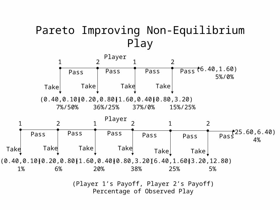
Pareto Improving Non-Equilibrium Play

(Player 1’s Payoff, Player 2’s Payoff)

7%/50% 36%/25% 37%/0% 15%/25%

5%/0%

1% 6% 20% 38% 25% 5%

4%

(0.40,0.10) (0.20,0.80) (1.60,0.40) (0.80,3.20)

(6.40,1.60)

Player1 2 1 2

Take

Pass

Take

Pass

Take

Pass

Take

Pass

Player

(0.40,0.10) (0.20,0.80) (1.60,0.40) (0.80,3.20) (6.40,1.60)

1 2 1 2

(3.20,12.80)

1 2(25.60,6.40)

Take

Pass

Take

Pass

Take

Pass

Take

Pass

Take

Pass

Take

Pass

Percentage of Observed Play