Embed Size (px)
Citation preview
Static and Dynamic Networks in Interbank Markets
Ethan Cohen-Cole∗
Econ One Research
Eleonora Patacchini
Cornell University
Yves Zenou
Stockholm University and IFN
This version: December 18, 2014
Abstract
This paper proposes a model of network interactions in the interbank market. Our
innovation is to model systemic risk in the interbank network as the propagation of
incentives or strategic behavior rather than the propagation of losses after default.
Transmission in our model is not based on default. Instead, we explain bank prof-
itability based on competition incentives and the outcome of a strategic game. As
competitors’ lending decisions change, banks adjust their own decisions as a result:
generating a ‘transmission’ of shocks through the system. We provide a unique equi-
librium characterization of a static model, and embed this model into a full dynamic
model of network formation. We also determine the key bank, which is the bank that
is crucial for the stability of the financial network.
Keywords: Financial networks, interbank lending, interconnections, network cen-
trality, key banks.
JEL Classification: G10, C21, D85.
∗Ethan Cohen-Cole: Managing Director, Econ One Research. 2040 Bancroft Ave #200. Berkeley, CA94708, USA. Email: [email protected]. Eleonora Patacchini: Cornell University, Department of Eco-
nomics, Ithaca, NY 14853, USA. Email: [email protected]. Yves Zenou: Stockholm University, Department
of Economics, 106 91 Stockholm, Sweden. E-mail: [email protected]. We are very grateful to the Editors
and two anonymous reports for helpful comments. We also thank Carefin — Bocconi Centre for Applied
Research in Finance for financial support. Cohen-Cole also thanks the CIBER and the US Department of
Education for support. All errors are our own.
1
1 Introduction
Since the onset of the financial crisis in 2007, the discourse regarding bank safety has shifted
strongly from the riskiness of financial institutions as individual firms to concerns about
systemic risk.1 As the crisis evolved, the public debate did as well, with concerns about
systemic risk evolving from too-big-to-fail (TBTF) considerations to too-interconnected-to-
fail (TITF) ones. The academic and policy literature has followed, with the growth of papers
that discuss network linkages in the financial system.2 This literature’s largest success has
been identifying and describing the properties of financial networks. Prior to the crisis,
most observers knew that financial institutions were connected, and that knowledge has now
expanded to recognize, for example, that the banking system is largely tiered, that the CDS
market exhibits small-world properties (Peltonen et al, 2013), and that the largest 50 or so
institutions in the EU are highly connected (Alves et al, 2013). A variety of other papers
find similar features in other markets and sub-components of the same markets (see Alves
et al 2013 for a good review of recent literature).
A second success of the recent literature is a schematic linking of network properties and
patterns to economic outcomes. By successfully appropriating the terminology and methods
of other fields and applying them to the graph of various financial markets, we are beginning
to learn the broad correlations between networks and outcomes. For example, one can look
at the structure of the network before, during and after the crisis and then correlate the
observed economic outcomes with the network structure. See for example Puhr et al (2012)
and Fricke and Lux (2012). The former shows changes through the crisis and the latter
stability, though they treat different markets.
1Indeed, there is a wide range of research on the importance of interbank markets, including some that
address the systemic risk inherent to these markets. Some examples include Freixas et al. (2000), Iori and
Jafarey (2001), Boss et al (2004), Furfine (2003), Iori et al. (2006), Soramäki et al. (2007), Pröpper et al.
(2008), Cocco et al. (2009), Mistrulli (2011), and Craig and Von Peter (2010). Each of these discuss some
network properties or discuss the importance of these markets to systemic risk evaluation.2A general perception and intuition has emerged that the interconnectedness of financial institutions is
potentially as crucial as their size. A small subset of recent papers that emphasize such interconnectedness
include Acemoglu et al. (2012), Adrian and Brunnermeier (2009), Allen et al. (2012), Amini et al. (2010),
Boyson et al. (2010), Cabrales et al. (2013), Cohen-Cole et al. (2014), Danielsson et al. (2009) and Elliott
et al. (2014).
2
Finally, a third branch of research has undertaken the difficult task of modeling the
economics that drive agent participation in the network. The current financial networks
literature is largely based on random network and preferential attachment models which both
use models from the applied mathematics and physics literature (Albert and Barabási 2002;
Easley and Kleinberg 2010; Newman 2010). The preferential attachment model (Barabási
and Albert 1999) is effectively based on a random network approach, since agents form links
in a probabilistic way leading to more popular nodes being more likely to be chosen (the so-
called rich-get-richer model). To this class of models belong simplified networks with simple
shocks, including models of cascading default.
This paper has two goals. First, we seek to add to a portion of the field that has received
little attention - the link between propagation of financial risk and agent incentives on a
network. It is well known and accepted that banks act strategically given the market and
regulatory incentives they face. We apply the new methods of optimization in networks
(Goyal 2007; Jackson 2008; Jackson and Zenou 2014) to the interbank market with a point-
in-time spatial model of homogeneous banks and no defaults. Using these methods, we are
able to precisely identify the equilibrium quantity of lending attributable to the network
structure.
The closest papers to our in the literature are Acemoglu et al. (2012) and Elliott et
al. (2014), as well as an earlier paper by Gai and Kapadia (2010). These papers explore
the propagation of shocks in financial institutions networks. Networks in these papers are
debt holdings or interbank lending, and shock propagation originates from an institution’s
failure to pay some or all of its debts. The three papers’ principal results reflect a spectrum
of potential shocks from small to huge. Acemoglu et al. (2012) focus on the extremes and
Elliott et al. (2014) highlight that intermediate cases can be particularly worrysome. These
papers also discuss the gamut of network structures in terms of the consequences of shocks.
Gai and Kapadia (2010) highlight that the location of a shock and connectivity of a network
will impact the outcome of a shock. Elliott et al. (2014) add a dimension to the analysis by
including the level of cross-holdings of the network in addition to diversification of holdings.3
3While we don’t explore in this paper, our paper shares with Elliot et al. (2014) the possibility of non-
monotonicity of impact from shocks. They occur in our model due to the generalizability of network structure
3
We complement this line of research by exploring a different dimension of shocks - ones
that do not emerge from a bankruptcy or other failure to pay. Instead, we explore shocks
that occur as a result of financial incentives in the absence of default. Financial institutions
regularly adjust market participation. Indeed, markets are characterized by increasingly fast
reoptimizations of portfolios and asset holdings. These changes have lightning-fast impacts;
as a result, changes in bank incentives can lead to changes in holdings long before any defaults
take place or even in the complete absense of defaults. Bank runs and repo runs are simple
examples of the potential adverse consequences of these actions.
By describing the bank optimization without default, we can then determine the impact
on the network structure itself. In addition to being able to comment on the extant properties
of different network structures, the model here can link the network structure to specific bank
incentives and behaviors. For policy makers, this linkage is crucial. Much as competition
regulators need an understanding of the behavior of market participants in order to make
informed policy decisions as to the regulation of a given industry, a bank regulator must have
information on bank behavior and incentives in order to make policy decisions. Our paper is
among a relatively small set of papers to both explicitly model a set of bank behaviors and
describe how behaviors change as a function of a complex market structure.
Our second goal is to use the description of bank behavior within a network to illus-
trate how an understanding of this behavior can be formalized into a measure of systemic
risk. In particular, we provide a measure that formally links the structure of a network to
the propagation of incentives. We again look at a system without defaults, and illustrate
how small changes in uncertainty, risk, or behavior can propagate through a network; this
propagation leads to changes in volumes and prices in concrete and measurable ways. In-
deed, we provide a closed form solution for each. This propagation is well understood from
an institutional perspective; what remains is to link this type of phenomenon explicitly to
network theoretical tools so that these phenomena can be understood structurally. Institu-
tionally, there is broad acceptance of the presence of contagion effects; fear of risk can spread
rapidly in a variety of forms. The structural view is important because the exact topology
and in Elliot et al. (2014) because of the presence of two dimensions of network connectivity.
4
of the network can fundamentally alter incentives and prices. Much in the same way that
Elliott, Golub and Jackson (2014) calculate how particular network structures can be linked
to particular default cascades, we provide a mechanism to link a shock without default to
particular cascades. This provides a measure of total systemic risk, as well as illustrates a
method to calculate the contribution of individual banks to this total. Importantly, both of
these measures emerge directly from the optimization problem of banks.
To further capture the fact that financial networks are rapidly changing, we take the
modeling exercise another step forward. As shocks hit a system, the existing pattern of
network links will evolve over time. As such, reduced form and/or static spatial models of
systemic risk may be insufficient for understanding the importance of interconnectedness on
financial markets. With this in mind, we explicitly embed our static model into a complete
dynamic model of network formation. Thus, we are able to characterize not only the equilib-
rium pattern of behavior at each point in time, but also describe how this behavior evolves
over time. As banks form and break links, the structure of the network will change, and the
nature of systemic risk with it. Our model is useful in that we can discuss how systemic
events emerge even in the absence of defaults (e.g. runs on the bank, flights to quality, etc.).
Once we have developed the static and dynamic models, we look at the impact of the
removal of a bank from the network on total activity. We derive an exact formula for the
“key bank”, i.e. the bank which once removed from the network reduces total activity (here
total volume of loans) the most. This policy can help a regulatory authority (such as the
European Central Bank) to decide which bank should be bailed out in case of a financial
crisis.
2 Static Model
2.1 Notation and model
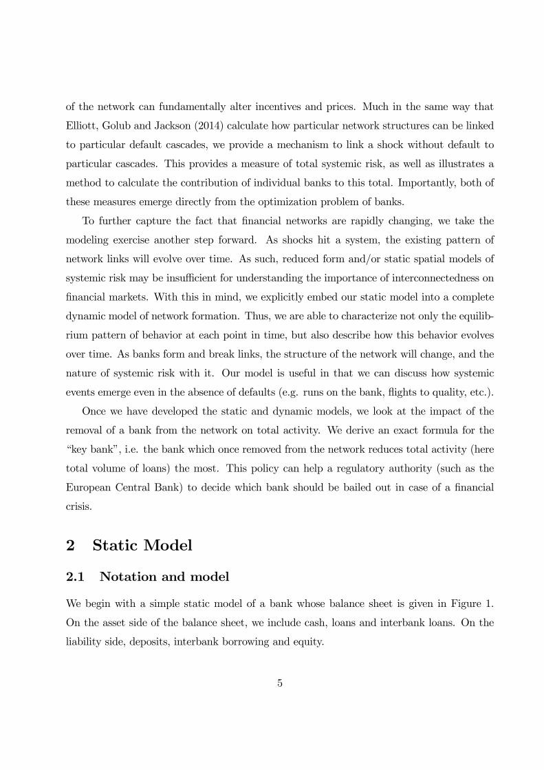
We begin with a simple static model of a bank whose balance sheet is given in Figure 1.
On the asset side of the balance sheet, we include cash, loans and interbank loans. On the
liability side, deposits, interbank borrowing and equity.
5
Assets Liabilities
Cash Deposits
Equity = eiInterbank loans = qi
Loans Interbank borrowing
Figure 1: Balance sheet
Our primary object of interest will be either interbank loans or interbank deposits. In
addition, we specify a basic leverage constraint for each bank as:
≥
where is the equity of bank and is the leverage constraint. For simplicity, we group
cash and loans into a single variable (i.e. loans + cash = ). Then we can write that
interbank loans at each point in time must satisfy two criterion. One, given a value for
liabilities and for ,
= −
The equality condition simply means that banks must match assets and liabilities. The
assumption that interbank loans are the remaining choice on the balance sheet reflects the
nature of this market. Precise deposits balances are determined by customer preferences,
non-interbank loans are typically much longer maturity and cannot be underwritten or sold
on a moment’s notice with any reliability, and equity takes weeks or months to issue. Thus,
in the perspective of a day or two, one of the only free variables for a bank to clear its balance
sheet is the interbank market.4
4We abstract for now from the ability to borrow from the central bank. This is an alternate mechanism
6
Two, the leverage constraint requires that
≥ + (1)
This reflects the fact that banks cannot lend funds greater than some multiple of their equity.
For example, in the 2000s, European banks were not bound explicitly by a leverage constraint.
However, Basel capital constraints formed a type of upper bound on the quantity of lending
possible. We include this feature particularly because new Basel III regulations explicitly
discuss additional capital requirements for Systemically Important Financial Institutions
(SIFIs). The borrowing side obviously has no such constraint.
As we develop the model, two key features will emerge: global strategic substitutability
and local strategic complementarities. These will show that, as total quantities in the market
increase, prices will fall. However, at the local level, between two agents, there will be an
incentive to increase prices when quantities increase due to the complementarity effect. The
model will find an equilibrium where these effects are balanced.
To our knowledge, the fact that we incorporate both local and global components adds
to the financial networks literature; by incorporating both the direct network influences as
well as the system-wide effects, our model is particularly suited to the description of financial
markets. These markets are influenced both by prices (global) and network impacts (local).
We look at a population of banks. We define for this population a network ∈ G as aset of ex-ante identical banks = {1 } and a set of links between them. We assumeat all times that there are least two banks, ≥ 2. Links in this context can be defined ina variety of ways. In other work, they have represented the exchange of a futures contract
(Cohen-Cole et al., 2014). In the banking networks that we study, the links will represent
the presence of a interbank loan. This means, in particular, that the network is directed
because bank may make a loan to bank (there is thus a link between them) while bank
may not make a loan to bank .
In the language of graph theory, in a directed graph, a link has two distinct ends: a
head (the end with an arrow) and a tail. Each end is counted separately. The sum of
to match the balance sheet. However, this type of borrowing typically comes at a penalty rate. We return
to penalty rate borrowing in the policy section at end.
7
head endpoints count toward the indegree and the sum of tail endpoints count toward the
outdegree. Because here we consider loans between banks, we will only consider outdegrees.
Formally, we denote a link from bank to bank as = 1 if bank has given a loan to
bank , and = 0, otherwise. The set of bank ’s direct links is: () = { 6= | = 1}.The cardinality of this set is denoted by () = |()|. In other words, the outdegree ofbank , denoted by (), is the number of loans bank has given, that is () =
P .
The −square adjacency matrix G of a network keeps track of the direct connections in
this network. Because the network is directed, G is asymmetric.5
We hypothesize that these direct links produce a reduction in costs of the collaborating
banks. In other words, we assume that a financial institution’s cost of doing business is
lowered through their financial connections to other institutions, and by their neighbors
doing more business. Although the following is outside the model, it is intuitive that if a
financial institution has a neighbor that does a lot of business, that institution will be
able to lend money more reliably to when requires it, reducing the cost to of using
the interbank market to make up balance sheet shortfalls. This creates a new mechanism
through which shocks can be transmitted. We believe that this mechanism is particularly
appealing because it provides a natural motivation for financial connections to be established
and can also help explain the observed structure of the interbank market.
This assumption seems to be strongly supported empirically. Treasury operations for a
small deposit-taking entity with a single link typically consist of a daily phone call from
the bank CFO to a regular, and typically much larger, counterparty to arrange to lending
to the larger counterpary. For example, in the case of e-MID,6 the small bank must incur
the fixed costs of participating even though it has only a single link. These operations are
expensive to maintain as it takes the direct participation of senior management of the small
bank to generate the loan. As banks increase their connections; however, the average unit
costs associated with managing a treasury operation strongly decrease in the number of
5Vectors and matrices will be denoted in bold and scalars in normal text.6The e-MID SPA (or e-MID) was the reference marketplace for liquidity trading in the Euro area during
the period 2002-2009. It was the first electronic marketplace for interbank deposits (loans), a market that
has traditionally been conducted bilaterally.
8
counterparties. Some evidence for this is seen in the fact that only a few banks serve as
de-facto moneycenter banks. These institutions are capable of managing a multiplicity of
links because of the high fixed and low average cost per counterparty.
We will model the quantity choice (i.e. volume of loans) based on competition in quanti-
ties of lending a la Cournot between banks with a single homogenous product (a loan). We
do not model the borrowing market but our analysis would be the same if we only focused on
borrowers and not lenders. The distinction between lenders and borrowers is useful for three
reasons. First, it allows us to look separately at what happens to each side of the market.
Second, it allows us to use well-established competition frameworks, such as Cournot which
are based on the idea of a group of firms competing for customer business. Looking only at
one side of the market (here interbank loans) allows this view. Third, looking at each side
of the market individually reflects the fact that we need gross lending amounts to under-
stand competitive forces. If a bank borrows $100 and lends $99, to understand the network,
we need to know both quantities; a netted $1 borrowing does not capture the complexity
and scale of the interactions. Recall that we will precisely identify which banks lend to and
borrow from which other banks.
We assume the following standard linear inverse market demand where the market price
is given by:
= −X∈
(2)
where 0. This means that we assume that the loan market is integrated since there is a
single market-clearing price and each bank is path-connected with any other bank (network
component). This is true in the interbank market, for example the e-MID market. As stated
above, we only look at one side of the market. If we analyze the lenders’ behavior only, then
determines the price (interest rate) of loans between banks. If we study the borrowers’
behavior, then reflects the price of borrowing between banks. Observe that issues like the
riskiness of the lenders or borrowers are ignored here. As stated above, in this paper, we
focus on the lenders’ behavior.
The marginal cost of each bank ∈ is (). The profit function of each bank in a
9
network is therefore given by:
() = − ()
= −X∈
− ()
where is the loan quantity produced by bank . We assume throughout that is large
enough so that price and quantities are always strictly positive.
Our specification of inter-related cost functions is as follows. The cost function is assumed
to be equal to:
() = 0 −
"X
=1
#(3)
where 0 0 represents a bank’s marginal cost when it has no links while 0 is the cost
reduction induced by each link formed by a bank. The parameter could be bank specific
as well so that , but for simplicity of notation, we do not report this case.
Equation (3) means that the marginal cost of each bank is a decreasing function of
the quantities produced by all banks 6= that have a direct link with bank . As stated
above, this is because the operational costs of a trading floor or treasury operation decline
per dollar of loan as loan size increases. This is the specification that drives the functional
relationships between banks.
To ensure that we obtain a reasonable solution, we assume that 0 is large enough so that
() ≥ 0, ∀ ∈ , ∀ ∈ G. The profit function of each bank can thus be written as:
() = − ()
= −X∈
− 0 +
X=1
= − 2 −X 6=
+
X=1
(4)
where ≡ − 0 0.
We highlight a few features of equation (4). First, we can see that profits are a negative
function of total loans. This we call global strategic substitutability, as the effect operates
10
only through the market and not through the direct links that form the network. So as
increases,()
is reduced as demand falls.
Second, we can see that profit is increasing in the quantity of direct links, via the cost
function impact. This we refer to as local strategic complementarities since if is linked with
, then if increases()
is increased because of the reduction in the cost. Total profits
are of course, dependent on the two jointly.
Third, we can define as the cross partial of profitability with respect to a bank’s
quantity change and another bank’s quantity change. We have:
=2()
=
( = −1 + if = 1
= −1 if = 0(5)
so that ∈ { }, for all 6= with ≤ 0.This last feature highlights the mechanism of the model. A shock to a connected bank
changes the incentives of a bank to lend, precisely through the function (5). Notice that
the model generates systemic risk insofar as shocks that impact a given bank, such as an
exogenous decrease in capital and ability to lend, pass through to the rest of the market
through a competition mechanism. The global effect of the reduction in lending by a single
bank is an increase by others. The local effect, however, that passes through the network
linkages, is that costs increase. As a result, loan volumes of direct network links decline as
well. Once network links change their choices, their links do so as well, and so on.
This dual effects and implicit tradeoffs have policy implications. Competition in a net-
work context / connected industries requires an understanding of how firms’ interconnections
impact their pricing and volume decisions. These linkages can lead to local cascades and
reductions in total lending even when the system as a whole is not at risk.
2.2 Equilibrium loans
Consider a Cournot game in which banks choose a volume of interbank lending conditional
on the actions of other banks. This game requires common knowledge of the actions of other
banks. Agents have the defined profit function in (4), which implies that cost is intermediated
by the network structure.
11
It is easily checked that the first-order condition for each bank is given by:
∗ = −=X=1
+
X=1
(6)
We now characterize the Nash equilibrium of the game. Denote by b ( ) the ( ×1) vector of Katz-Bonacich centralities, which is formally defined in Appendix 1. For all
b( )∈IR, denote ( ) = 1 ( ) + + ( ) as the sum of its coordinates.
Proposition 1 Consider a network game where links are represented by loans between
banks and where the profit function of each bank is given by (4). Then this game has a
unique Nash equilibrium in pure strategies if and only if (G) 1. This equilibrium q∗ is
interior and given by:
q∗ =
1 + ( )b ( ) (7)
The equilibrium profit is then given by:
∗ = (∗ )2=
22 ( )
[1 + ( )]2 (8)
This result is a direct application of Theorem 1 in Ballester et al. (2006). Appendix
2 shows in more detail how the first order condition can be written as a function of Katz-
Bonacich centrality. It also provides an example.
This solution is useful for a couple of reasons: One, notice that this equation provides a
closed form solution to the game with any number of banks and to calculate output, only
the matrix of interconnections G and the bank specific cost functions are needed. Two, this
equation provides the basis for estimation of any network linked bank decision. We explore
this implication in more detail below in Section 3.
A key parameter in this equilibrium result is , the coefficient in the equation (18) that
measures how much of a shock to a given bank is passed on to connected banks. While we
don’t explore in this paper, our paper shares with Elliot et al. (2014) the possibility of non-
monotonicity of impact from shocks. They occur in our model due to the generalizability
of network structure and in Elliot et al. (2014) because of the presence of two dimensions
of network connectivity. The equilibrium in our model is a measure of the pass-through
12
rate, but notice that diverse network structures lead to potentially widely diverse impacts
of shocks that depend on the location and severity of the shock as well as the structure of
the network.
To illustrate this issue, denote by ∗ the Nash equilibrium in loan quantities where
there is no network and by ∗ the same quantity where banks are connected by a network
(defined by (7). We have the following result, which proof is given in Appendix 3.
Proposition 2 Assume that (G) 1. Then,
∗ = ∗
+
(1 + )
"
X=1
∗ −
X 6=
X=1
∗
# (9)
In the case of a dyad, i.e., we have:
∗ =3
(3− )∗ (10)
Proposition 2 illustrates that is a multiplier and, in our context, is a measure of systemic
risk that propagates risk through incentives. The intuition of equation (9) is clear. Total
output is higher with networks than without networks and the difference is measured as
∗ − ∗ =¡
1+
¢P
=1
P
=1 ∗ 0. In other words, total lending increases by this
value when network effects are present. This implies that prices of loans are much lower with
networks since ∗ = ∗+¡
1+
¢P
=1
P
=1 ∗ , which creates even more interactions
(i.e. loans). As a result, profits are also higher with networks. The implications is clear. In
normal times, the system relies on network structure to boost lending and profits - without
the network, both would be lower. As a result, even in the absence of any actual losses,
shocks to structure are costly in part because they unwind this benefit at a rapid pace. We
continue this notion by articulating a measure of system risk that measures the system’s
fragility vis-a-vis the collapse or contraction of the network benefit.
In (10), we consider the dyad, i.e. the case of two banks and ( = 2). In that case,
the multiplier is equal to 3 (3− ) 1. One can see that this multiplier increases in
so that the higher is , the higher is the quantity of loans that will be given to each bank.
This means, in particular, that if there is a shock to this economy, , the systemic risk, will
propagate the risk at a factor of 3 (3− ). In other words, if for example = 05, then
13
an isolated bank will provide a volume of loans equal to ∗ while if it has only a single
connection, its volume increases by 20%.
2.3 Equilibrium prices
One of the powerful features of the model is that it provides a structural link between the
network pattern and the equilibrium market price for interbank loans. Changing the network
structure changes equilibrium prices. Indeed, this is true because these prices incorporate the
network benefit. Throughout this paper, our cost function is closely related to our findings.
We emphasize this tight relationship between a cost function and the incentives to lend in
a financial network not because this is the sole possible description of the market. Instead,
it enables us to illustrate the fact that incentives impact prices / volumes through network
architecture in a clear and measureable way. This can be observed through two features of
the model. First, the equilibrium quantity for each bank is expressed precisely in (7). As
the sum of these quantities change, the global effect, as in any market, will be to influence
prices. This is what we labeled global strategic substitutability, above. Two, the individual
patterns of links in the network will influence the local loan decisions. These local strategic
complementarities also influence aggregate prices.
To be more precise, using the linear inverse market demand (2) and (7), we obtain the
following equilibrium price of loan transactions:
∗ = −X∈
∗ = − ( )
1 + ( )(11)
where = ( − 0).
Example 1 Consider the two following directed networks:
14
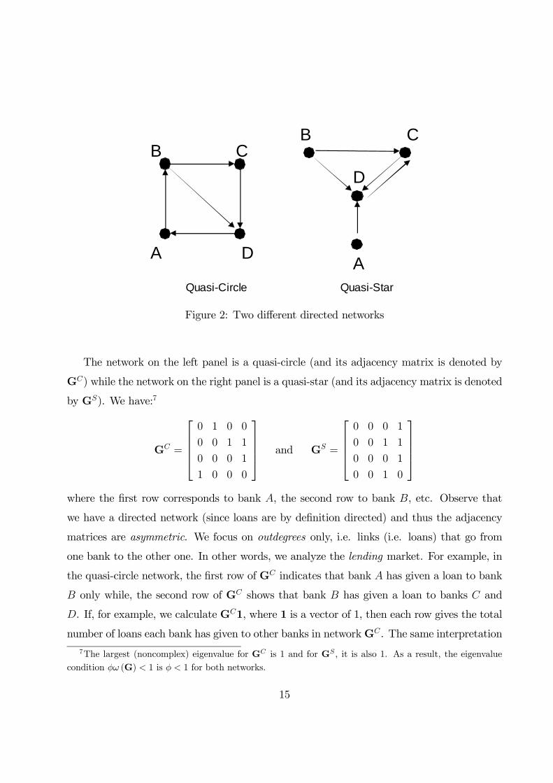
Quasi-Circle Quasi-Star
A
B C
D
D
A
B C
Figure 2: Two different directed networks
The network on the left panel is a quasi-circle (and its adjacency matrix is denoted by
G) while the network on the right panel is a quasi-star (and its adjacency matrix is denoted
by G). We have:7
G =
⎡⎢⎢⎢⎣0 1 0 0
0 0 1 1
0 0 0 1
1 0 0 0
⎤⎥⎥⎥⎦ and G =
⎡⎢⎢⎢⎣0 0 0 1
0 0 1 1
0 0 0 1
0 0 1 0
⎤⎥⎥⎥⎦where the first row corresponds to bank , the second row to bank , etc. Observe that
we have a directed network (since loans are by definition directed) and thus the adjacency
matrices are asymmetric. We focus on outdegrees only, i.e. links (i.e. loans) that go from
one bank to the other one. In other words, we analyze the lending market. For example, in
the quasi-circle network, the first row of G indicates that bank has given a loan to bank
only while, the second row of G shows that bank has given a loan to banks and
. If, for example, we calculate G1, where 1 is a vector of 1, then each row gives the total
number of loans each bank has given to other banks in networkG. The same interpretation
7The largest (noncomplex) eigenvalue for G is 1 and for G , it is also 1. As a result, the eigenvalue
condition (G) 1 is 1 for both networks.
15
can be made for G. Observe also the two networks have the same total number of banks
(4) and have the same total numbers of loans (5) but have a different structure.
In this framework, the Katz-Bonacich centrality is a measure of “popularity” since the
most central bank (i.e. node) is the one that makes the higher number of loans (i.e. links).
Fortunately, the symmetry of the adjacency matrix does not play any role in the proof
of Proposition 1 and thus the results are true for both directed and undirected networks.
We can see here how prices vary as a function of even relatively small changes in network
structure. Using Proposition 1, the unique Nash equilibrium is given by:⎡⎢⎢⎢⎣∗∗∗∗
⎤⎥⎥⎥⎦ = ( − 0)
5 + 5+ 62 + 23 − 4
⎡⎢⎢⎢⎣1 + + 22 + 3
1 + 2+ 22 + 3
1 + + 2
1 + + 2 + 3
⎤⎥⎥⎥⎦for the quasi-circle network and⎡⎢⎢⎢⎣
∗∗∗∗
⎤⎥⎥⎥⎦ = ( − 0)
5
⎡⎢⎢⎢⎣1
1 +
1
1
⎤⎥⎥⎥⎦for the (quasi)star-shaped network. The quasi-circle network where bank has the highest
Katz-Bonacich centrality (and thus provides the highest number of loans) is less symmetric
than the (quasi)star-shaped one. Bank is the second most active bank because it provides
a loan to - followed by bank and then bank . On the contrary, for the quasi-star
network, banks , , and provide the same number of loans while bank has the highest
Katz-Bonacich centrality. This is because they all lend to the same bank, .
What is interesting here is the impact of network structure on the aggregate equilibrium
price of loans. In the circle network, each loan is priced at
∗ =
¡1− 3 − 4
¢ + (4 + 5+ 62 + 33)0
5 + 5+ 62 + 23 − 4
where is the market demand from equation (2) and is the coefficient in the equation (18).
For the star-shaped network, we obtain:
∗ =(1− ) + (4 + ) 0
5
16
As a result, with four banks , , and , depending on the network structure, the price
for loans can differ. Indeed, it is easily verified that ∗ ∗. This reflects the fact that the
quasi-star network induces less competition and thus less loan output than the quasi-circle
network. This example also highligts that cost complementarities are the key force behind
the impact of networks on competition.
2.4 Equilibrium behavior with leverage constraints
Remember that we have a leverage constraint given by (1). We need to check that the Nash
equilibrium satisfies this condition. Define ≡ − . Since , and are purely
exogenous variables, we consider three possibilities.
Proposition 3 Assume that (G) 1. Then,
() If no banks are constrained by the leverage constraint, i.e., the equilibrium quantity of
loans ∗ , defined by (7), is such that ∗ ≤ , for all = 1 , then all banks play the
Nash equilibrium quantity of loans ∗ defined by (7).
() If all banks are constrained so that ∗ , for all = 1 , in equilibrium, all banks
provide loans equal to ∗ = ≡ −.
() If some banks are constrained by the leverage constraint and some are not, then banks
for which ∗ ≤ will provide loans made by ∗ , defined in (7), while those for which
∗ , will provide ∗ = ≡ −.
This difference between constrained and unconstrained suggests that increasing the frac-
tion of constrained banks leads to a smaller fraction of banks propagating incentives through
the network. This can have a range of potential impacts on total systemic risk and the
allocation of risk in the system. Indeed, when increases, more and more banks are con-
strained in their loan possibilities and are more likely to hit the leverage constraint so that
∗ = ≡ −. Interestingly, this depends on the network structure so that the same
bank with the same leverage constraint can behave differently depending on the network it
17
belongs to. Consider again Example 1 (Figure 2) and assume for bank that8
( − 0)¡1 + + 2
¢5 + 5+ 62 + 23 − 4
( − 0)
5
This implies that ∗ and ∗ and thus, in equilibrium,
∗ =( − 0)
¡1 + + 2
¢5 + 5+ 62 + 23 − 4
and ∗ = ≡ −
In other words, the same bank in the quasi-circle network will provide its Nash equilibrium
quantity of loans, but in the star-shaped network will hit the leverage constraint and will
lend loans so that ∗ = . This is true for a given . When increases then banks are
more likely to hit the leverage constraint and will not provide their “optimal” (i.e. Nash
equilibrium) quantity of loans. The policy implication is that leverage constraints limit
lending not only via directly constrainted banks by also by an addiitonal amount as these
restrictions propagate through the network.
3 Framework for empirical analysis
We begin by defining a network of banks. Banks conduct transactions with other banks
nearly continuously; as such, we make an assumption about what defines a network. Since
the vast majority of transactions are overnight transactions and banks use the interbank
loan market for rectifying deposit imbalances, one can surmise that a reasonable network is
characterized by the transactions that occur in a short time frame. A one-day time period
is a natural time period to start with. That said, many overnight interbank loans are rolled
over the following day. While the lending bank typically has the option to withdraw funding,
the persistence in relationships implies that the networks that determine lending choices may
be slightly longer than a day. We will use one day as a benchmark measure of networks.
8Observe that, since 1, we have:
( − 0)¡1 + + 2
¢5 + 5+ 62 + 23 − 4
( − 0)
5
18
Further supporting the use of a short-term network measure, the model above takes the
interbank lending/borrowing decision as the tool to balance the bank’s assets and liabilities,
taking the remainder of the balance sheet as given. Once we consider other assets and
liabilities with longer maturities, alternate network measures may be important.
Assume that there are networks in the economy, defined by the number of days. Each
network contains banks. We can then estimate the direct empirical counterpart of the
first-order condition in the static model above, equation (6):
= + 1
X=1
+ , for = 1 ; = 1 (12)
where = 12 − 1
2
P
=1 6= This equation indicates that the equilibrium quantity choice
of a bank is a function of quantity choices of others in the same market. We denote as
the lending or borrowing of bank in the network ; =P
=1 is the number
of direct links of ; 1
P=1 is a spatial lag term; and is a random error term.
The spatial lag term is equivalent to an autoregressive term in a time regression: a length-
three connection in this model through lending connections is akin to a three period lag in a
time series autoregressive model. This model is the so-called spatial lag model in the spatial
econometric literature and can be estimated using Maximum Likelihood (see, e.g. Anselin
1988).
4 Dynamic Model
In this section, we extend the model set out in Section 2 to include strategic link formation
amongst banks. This step is crucial in that it permits us to include in our analysis not only
the quantity and price choices amongst banks conditional on their existing network, but also
their decisions on how to change the network structure itself. The model here will show the
equilibrium outcome network structure conditional on these strategic choices. Such a model
gives us the ability to validate that our static model results are reasonable insofar as they are
not contradicted by strategic network formation incentives. It also allows us to investigate
how strategic behavior can impact network structure and liquidity availability.
19
Our central modeling assumptions will be that links are formed based on the profitability
tradeoff that emerges from the game in the static model. Effectively, banks know that the
game will be played in the subsequent period and that all other banks are also making
network formation decisions. Based on these, banks can choose whether or not to form a
link; that is, to make a loan to a new bank. We will also specify an exogenous probability
of link formation, .9
To describe the network formation process we follow König et al. (2014a). Let time be
measured at countable dates = 1 2 and consider the network formation process (())∞=0
with () = (()) comprising the set of banks = {1 } together with the set oflinks (i.e. loans) () at time . We assume that initially, at time = 1, the network is empty.
Then every bank ∈ optimally chooses its quantity ∈ R+ as in the standard Cournotgame with no network. Then, a bank ∈ is chosen at random and with probability
∈ [0 1] forms a link (i.e. loan) with bank that gives it the highest payoff. We obtain
the network (1). Then every bank ∈ optimally chooses its quantity ∈ R+, and thesolution is given by (7). The profit of each bank is then given by (8) and only depends on its
Katz-Bonacich centrality, that is, its position in the network. At time = 2, again, a bank
is chosen at random and with probability decides with whom she wants to form a link
while with probability 1− this bank has to delete a link if she has already one. Because
of (8), the chosen bank will form a link with the bank that has the highest Katz-Bonacich
centrality in the network. And so forth.
As stated above, the randomly chosen bank does not create or delete a link randomly. On
the contrary, it calculates all the possible network configurations and chooses to form (delete)
a link with the bank that gives it the highest profit (reduces the least its profit). It turns out
that connecting to the bank with the highest Katz-Bonacich centrality (deleting the link with
the agent that has the lowest Katz-Bonacich centrality) is a best-response function for this
bank. Indeed, at each period of time the Cournot game described in Section 2 is played and
it rationalizes this behavior since the equilibrium profit is increasing in its Katz-Bonacich
9While we don’t discuss in detail, this asssumption can be relaxed in a number of ways. For example,
König et al. (2010) show that a capacity constraint, what this model would interpret as a capital constraint,
generates similar network patterns.
20
centrality (see 8).
To summarize, the dynamics of network formation is as follows: At time , a bank is
chosen at random. With probability bank creates a link to the most central bank while
with complementary probability 1− bank removes a link to the least central bank in its
neighborhood.
Characterization of equilibrium We would like to analyze this game and, in par-
ticular, to determine, in equilibrium, how many links banks will have. More importantly,
we would like to describe the entire distribution of links for banks in the network. This
degree distribution gives the percentage of banks with number of links (degree) = 1 .
Recall that the decision to add or delete a connection to another bank is made based on
bank optimization decisions that emerge from our static model.
Our results follow the work in König et al. (2014a) who show that, at every period, the
emerging network is a nested split graph or a threshold network, whose matrix representation
is stepwise. This means that agents can be rearranged by their degree rank and, conditional
on degree 6= 0, agents with degree are connected to all agents with degrees larger than. Moreover, if two agents have degrees such that , this implies that their
neighborhoods satisfy N ⊂ N. Below, we will show how closely the theoretical patterns
implied by this model are replicated in the data.
Denote by ( ) the number of agents with degree ≤ 2 at time . It can be shown
that the dynamic evolution is given by:
( 0 + 1)−( 0) =
µ1−
¶(+ 1 0) +
(− 1 0)− 1
( 0) (13)
(0 0 + 1)−(0 ) =
µ1− 2
¶−
(0 ) +
µ1−
¶(1 ) (14)
These equations mean that the probability of adding connections to banks with degree is
proportional to the number of nodes with degree − 1 (resp. + 1) when selected for nodeaddition (deletion). The dynamics of the adjacency matrix (and from this the complete
structure of the network) can be directly recovered from the solution of these equations.
Since the complement of a nested split graph is a nested split graph, we can derive the
stationary distribution of networks for any value of 12 1 if we know the corresponding
21
distribution for 1−. With this symmetry in mind we restrict our analysis in the following
to the case of 0 ≤ 12. Let {()}∞=0 be the degree distribution with the -th element(), giving the number of nodes with degree in (), in the -th sequence () =
{()}−1=0 . Further, let () = () denote the proportion of nodes with degree and
let = lim→∞ E(()) be its asymptotic expected value (as given by ). In the following
proposition (König et al., 2014a), we determine the asymptotic degree distribution of the
nodes in the independent sets for sufficiently large.
Proposition 4 Let 0 ≤ 12. Then the asymptotic expected proportion of nodes in
the independent sets with degrees, = 0 1 ∗, for large is given by
=1− 21−
µ
1−
(15)
where
∗( ) =ln³(1−2)2(1−)
´ln¡1−
¢
These equations precisely define the equilibrium degree distribution in the interbank
market. The ability to reorganize - again based on incentives - allows one to understand how
policy interventions may impact dynamic outcomes.
5 Policy implications: Which bank is key?
In this section, we would like to use our static model of Section 2 to answer the following
questions: When one bank is taken out of the network, or when one bank is hit by a shock,
how do prices and quantities change? How does the network structure affect the answer?
Which networks are more or less resilient? Can a policy maker improve resilience to shocks
using some simple intervention. To address these questions, we will use the concept of “key
player” introduced by Ballester et al. (2006). If a regulatory authority such as the European
Central Bank, the Federal Reserve Bank or the Banque de France needs to decide which
bank should be bailed out because it is crucial for the “stability” of the bank system, then
this bank will be the key player or key bank. In other words, the key bank is the one whose
removal from the network would result in the largest reduction in total loan activity.
22
Formally, consider the previous model and denote by ∗() =X=1
∗ the total Nash
equilibrium level of loans in network , where ∗ is the Nash equilibrium loan quantity
produced by bank and given by (7). Denote also by [−] the network without bank .
Then, following Ballester et al. (2006), to determine the key bank, the planner will solve the
following problem:
max{∗()−∗([−]) | = 1 }
When the network is fixed, this is equivalent to:
min{∗([−]) | = 1 } (16)
Denote M( ) = (I−G)−1 so that the Katz-Bonacich centrality is defined as: b( ) =(I−G)−1 1. An element ofM( ) corresponding to the cell ( ) is denoted by .
Definition 1 Assume () 1. The intercentrality or key-player centrality measure
( ) is defined as follows:
( ) =[( )]
2
(17)
Ballester et al. (2006) derive the following result:
Proposition 5 A bank ∗ is the key player that solves (16) if and only if ∗ is the bank with
the highest intercentrality in , that is, ∗( ) ≥ ( ), for all = 1 .
The intercentrality measure (17) of bank is the sum of ’s centrality measures in , and
’s contribution to the centrality measure of every other bank 6= also in . It accounts
both for one’s exposure to the rest of the group and for one’s contribution to every other
exposure.
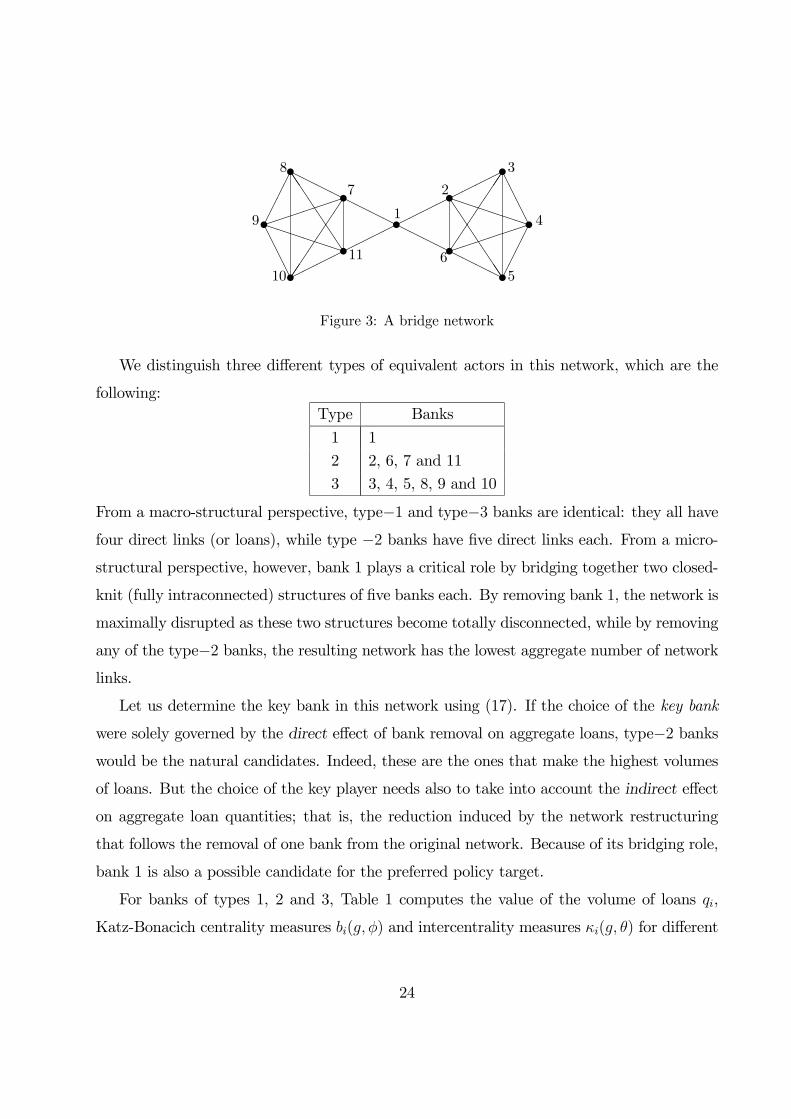
To understand this concept, consider the network described in Figure 3 with eleven
banks and three different types of players: 1, 2 and 3. This example was proposed by
Ballester et al. (2006). For the sake of the exposition, we look at an undirected network so
that if bank provides a loan to bank then the reverse is also true.
23
tt t
tt
1
3
2
6
4
5
HHHH
³³³³
³³
©©©©
JJJJJJJ
PPPPPPAAAA
¢¢¢¢
t©©
©©©©
©©HHHHHHHH
tt t
tt
8
7
11
9
10
¢¢¢¢
AAAA
³³³³
³³
PPPPPP
HHHH
JJJJJJJ
©©©©
Figure 3: A bridge network
We distinguish three different types of equivalent actors in this network, which are the
following:
Type Banks
1 1
2 2, 6, 7 and 11
3 3, 4, 5, 8, 9 and 10
From a macro-structural perspective, type−1 and type−3 banks are identical: they all havefour direct links (or loans), while type −2 banks have five direct links each. From a micro-
structural perspective, however, bank 1 plays a critical role by bridging together two closed-
knit (fully intraconnected) structures of five banks each. By removing bank 1, the network is
maximally disrupted as these two structures become totally disconnected, while by removing
any of the type−2 banks, the resulting network has the lowest aggregate number of networklinks.
Let us determine the key bank in this network using (17). If the choice of the key bank
were solely governed by the direct effect of bank removal on aggregate loans, type−2 bankswould be the natural candidates. Indeed, these are the ones that make the highest volumes
of loans. But the choice of the key player needs also to take into account the indirect effect
on aggregate loan quantities; that is, the reduction induced by the network restructuring
that follows the removal of one bank from the original network. Because of its bridging role,
bank 1 is also a possible candidate for the preferred policy target.
For banks of types 1, 2 and 3, Table 1 computes the value of the volume of loans ,
Katz-Bonacich centrality measures ( ) and intercentrality measures ( ) for different
24

values of and for = 1. In each column, a variable with a star identifies the highest
value.10
0.1 0.2
Bank Type
1 0077 175 292 0072 833 4167∗
2 0082∗ 188∗ 328∗ 0079∗ 917∗ 4033
3 0075 172 279 0067 778 3267
Table 1: Katz-Bonacich centralities versus intercentralities
First note that type−2 firms always display the highest Katz-Bonacich centrality mea-sures. These banks have the highest number of direct connections. Besides, they are directly
connected to the bridge bank 1, which gives them access to a very wide and diversified span
of indirect connections. Altogether, they are the most −central banks.For low values of , the direct effect on loan reduction prevails, and type−2 banks are
the key players −those with highest intercentrality measure . In other words, they are thecrucial banks in the system. When increases, however, the most active banks are no longer
the key players. There indirect effects matter a lot, and removing bank 1 from the network
results in the highest joint direct and indirect negative effect on aggregate loan volume.11
The individual Nash equilibrium loan quantities of the network game are proportional
to the equilibrium Katz-Bonacich centrality network measures, while the key player is the
bank with the highest intercentrality measure. As the previous example illustrates, these
two measures need not coincide. This is not surprising, as both measures differ substantially
in their foundation. Whereas the equilibrium-Katz-Bonacich centrality index derives from
strategic individual considerations, the intercentrality measure solves the planner’s optimal-
ity collective concerns. In particular, the equilibrium Katz-Bonacich centrality measure fails
to internalize all the network payoff externalities banks exert on each other, while the in-
tercentrality measure internalizes them all. More formally, the measure κ( ) goes beyond
10We can compute the highest possible value for compatible with our definition of centrality measures,
equal to b = 2
3+√41' 0 213.
11Note that the network [−1] has twenty different links, while [−2] has nineteen links. In fact, when is
small enough, the key player problem minimizes the number of remaining links in a network, which explains
why type−2 banks are the key player when = 01 in this example.
25
the measure b( ) by keeping track of all the cross-contributions that arise between its
coordinates 1( ) ( ).
Definition 1 specifies a clear relationship between ( ) and b( ). Holding ( )
fixed, the intercentrality ( ) of bank decreases with the proportion ( )( ) of
’s Katz-Bonacich centrality due to self-loops, and increases with the fraction of ’s centrality
amenable to out-walks.
It is important to understand the concept of key player in the interbank loan market.
The key bank or key player is the one whose exit will be the most costly for the system in
terms of total loan activity. However, the loss on total output (volume of loans) depends on
the systemic risk parameter , which measures the multiplier effects following the removal
of a bank.12 In other words, if, in the network of Figure 3, bank 1 would exit this market,
then the loss of total activity in terms of loans will be the highest. This is true only if is
high enough (here = 02) because, in that case, it will propagate beyond direct neighbors.
To illustrate this point, consider again the network in Figure 3. It is easily verified that,
when = 01, removing bank 1 leads to a decrease of 1751% of total loans quantities while
removing bank 2 leads to a decrease of 2012%. On the contrary, when = 02, these figures
are 8333% and 7857%, for bank 1 and 2, respectively.13 In other words, when = 02, if
bank 1 would exit from the interbank market, then the reduction in the total volume of loans
in this network will be as high as 8333%. This is because, when bank 1 exits the market, it
not only affects the banks it is directly linked with (banks 2, 6, 7 and 11) but also indirectly
affects all the other banks in the interbank market. The way it affects the other banks is
12In the peer-effect literature, is referred to as the social multiplier (see, in particular, Glaeser et al.,
2003; Jackson and Zenou, 2014; Liu et al., 2014).13Indeed, it easily verified that:
1 ( 01) ≡ ( 01)− ³[−1] 01
´= 19586− 16667 = 2919
2 ( 01) ≡ ( 01)− ³[−2] 01
´= 19586− 16305 = 3281
and
1 ( 02) ≡ ( 02)− ³[−1] 02
´= 91667− 50 = 41667
2 ( 02) ≡ ( 02)− ³[−2] 02
´= 91667− 51334 = 40333
26
proportional to the “distance” in the network and it is discounted by a factor of for banks
that are at a distance from bank 1.
We can now easily answer the questions we asked at the beginning of this section. First,
when a bank is taken out of the network, or when one bank is hit by a shock, we can
see now how prices and quantities change and how it depends on the network structure.
Indeed, using (2), we can analyze the effect on prices when a bank exits the market since, in
equilibrium,P∈
= ( ) [1 + ( )]. In fact, it is easily verified that the difference
in prices is inversely related to the difference in total quantities. For example, when = 02
and taking = 1, removing bank 1 or bank 2 from the market will lead to an increase of
8182% and 7711% in prices, respectively. It should also be clear that a policy maker can
improve the resilience to shocks using a simple intervention based on the identification of
the key bank. In a crisis setting, a policy maker would have additional rationale for support
to a key institution. Or conversely, it would have a pre-crisis rationale for re-arranging the
network importance to minimize the system’s dependence on a given institution. Finally,
network structure is also playing an important role since the key player will differ depending
on the network structure. For example, in a star-shaped network, the key player will always
be the central node, while, in other networks, like the one in Figure 3, it will depend on
the magnitude of the systemic risk . Indeed, to identify which networks are more or less
resilient is a more complicated question that refers to a network design policy (Belhaj et al.,
2014; König et al., 2014b). Given what we have shown here, it should be clear that regular
networks (such as the complete network or the circle) should be more resilient since the exit
of one bank from the market should have a relative lower impact on total activity since all
banks have the same activity (and all have the same Katz-Bonacich centralities).
6 Concluding remarks
We have constructed two models of the interbank loan market, a static and dynamic one.
Then, using these models, we have presented a measure of systemic risk in this market,
which is a precise measure of the aggregate liquidity cost of a reduction in lending by an
individual financial institution. This systemic risk measure is presented as an innovation vis-
27
a-vis existing approaches. It is based on the foundation of a microfounded dynamic model of
behavior. As well, it provides a tool to understand the transmission of shocks that extends
beyond default events and generalized price shocks. In the combination of these lies our tool;
the competitive responses made by banks generate the transmission of shocks in our model
and provide a tractable method of measuring and understanding systemic risk.
Our approach is designed to understand the role of network structure on interbank lend-
ing. As with any model, there are some limitations to the exercise. From a policy perspective,
we emphasize the utility of using a structural approach to networks. To the extent that the
model captures bank behavior, it allows policymakers the ability to test interventions with
an eye both to how banks will optimize in the short-run and how networks will form and
re-form under each assumption. We have also examined how a policymaker could monitor
more closely the key bank, which is the bank that is crucial for the stability of the financial
system.
An example is how one can interpret in our model with the imposition of the ECB’s
full allotment policy. This policy permitted banks to access credit lines from the ECB in
unlimited quantities at a fixed rate. We can model this by removing many higher risk banks
(or key banks) from the market. It is a straightforward result of the static model that the
removal will lower average demand in this market as well as reduce average risk.
A second example is the use of exceptional capital cushions for SIFIs. Our approach
allows one both to identify the SIFIs that are the largest contributors to systemic risk and
determine what occurs if these banks face increased, and now binding, capital constraints.
To identify the largest contributors, the static model indicates simply that the banks with
the highest Katz-Bonacich centrality are those with the highest contribution.
Using this information, an avenue for future research would be to evaluate optimal reg-
ulatory policy in the presence of networks. Given a particular objective function for the
regulator, such as minimizing volatility or minimizing total systemic risk, the approach here
could yield a set of capital constraints that solve the regulator’s problem. Notice that these
constraints would not necessarily have any of the cyclicality problems that a static, fixed
constraint does. For example, the regulator could optimize over contribution to systemic
28
risk over a period of time that includes recessions. Then, a capital cushion that depends on
the contribution to risk and position in the network would vary against the cycle.
We note in closing that the core assumption of our paper that cost is decreasing the
quantities of connections is central to our results. In other markets, and potentially in
subsections of the market we discuss, this reverse could be true. The network implications
would change if the cost function operated differently, but the insight that agent incentives
are a function of the market structure would remain intact. We leave exploration of the
details of this to future research.
References
[1] Acemoglu, D., A. Ozdaglar, and A. Tahbaz-Salehi (2012), “Systemic risk and stability
in financial networks,” mimeo.
[2] Adrian, T., and M. Brunnermeier (2009), “CoVaR,” Federal Reserve Bank of New York,
mimeo.
[3] Afonso, G., A. Kovner. and A. Schoar (2011), “Stressed, not frozen: The Federal funds
market in the financial crisis,” Journal of Finance 66, 4, 1109-39.
[4] Albert, R. and A.-L. Barabási (2002), “Statistical mechanics of complex networks,”
Review of Modern Physics 74, 47-97.
[5] Allen, F, A. Babus and E. Carletti (2012), “Asset commonality, debt maturity and
systemic risk ,” Journal of Financial Economics, 104, 519-534.
[6] Allen, F. and D. Gale (2000), “Financial Contagion,” Journal of Political Economy,
108,1-33.
[7] Alves, I, S. Ferrari, P. Franchini, J. Heam, P. Jurca, S. Langfield, F. Liedorp, A. Sanchez,
S. Tavolaro, and G. Vuillemey (2013), “The structure and resilience of the European
interbank market,” European Systemic Risk Board (ESRB) Occasional Paper No. 3.
29
[8] Amini, H., R. Cont, and A. Minca (2010) “Stress testing the resilience of financial
networks,” Unpublished manuscript, Columbia University.
[9] Anselin, L., (1988), Spatial Econometrics: Methods and Models, Boston: Kluwer Acad-
emic Publishers.
[10] Ballester, C., A. Calvo-Armengol, A. and Y. Zenou (2006), “Who’s who in networks.
Wanted: The key player,” Econometrica, 74, 1403-1417.
[11] Barabási, A.-L. and R. Albert (1999), “Emergence of scaling in random networks,”
Science 286 (5439), 509-512.
[12] Belhaj, M., Bervoets, S. and F. Deroïan (2014), “Using network design as a public
policy tool,” Unpublished manuscript, Aix-Marseille School of Economics.
[13] Bonacich, P. (1987), “Power and centrality: A family of measures,” American Journal
of Sociology, 92, 1170-1182.
[14] Boss, M., H. Elsinger, M. Summer and S. Thurner (2004), “Network topology of the
interbank market,” Quantitative Finance, 4:6, 677-684.
[15] Boyson, N., C. Stahel, and R. Stulz (2010), “Hedge fund contagion and liquidity shocks,”
Journal of Finance, 65, 1789-1816.
[16] Cabrales, A., P. Gottardi, and F. Vega-Redondo (2013), “Risk-sharing and contagion
in networks,” mimeo.
[17] Calvó-Armengol, A., E. Patacchini, and Y. Zenou (2009), “Peer effects and social net-
works in education,” Review of Economic Studies, 76, 1239-1267.
[18] Cocco, J., F. Gomes, and N. Martin (2009), “Lending relationships in the interbank
market,” Journal of Financial Intermediation, 18, 1, 24-48
[19] Cohen-Cole, E., A. Kirilenko, and E. Patacchini (2014), “Trading network and liquidity
provision,” Journal of Financial Economics, forthcoming.
30
[20] Craig, B. and G. Von Peter (2010) “Interbank Tiering and Money Center Banks,” FRB
of Cleveland Working Paper No. 10-14.
[21] Danielsson, J., H. Shin, J-P. Zigrand (2009), “Risk appetite and endogenous risk,”
Mimeo.
[22] Debreu, G. and I.N. Herstein (1953), “Nonnegative square matrices,” Econometrica 21,
597-607.
[23] Easley, D. and J. Kleinberg (2010), Networks, Crowds, and Markets: Reasoning About
a Highly Connected World, Cambridge: Cambridge University Press.
[24] Elliott, M.L., Golub, B. and M.O. Jackson (2014), “Financial networks and contagion,”
American Economic Review 104, 3115-3153.
[25] Farboodi, M. (2014): “Intermediation and Voluntary Exposure to Counterparty Risk,”
Mimeo.
[26] Freixas, X., B. Parigi, and J. Rochet, (2000), “Systemic Risk, Interbank Relations and
Liquidity Provision by the Central Bank,” Journal of Money, Credit and Banking 32,
611-638.
[27] Fricke, D. and Lux, T. (2012), “Core-periphery structure in the overnight money market:
Evidence from the e-MID trading platform”, Kiel Institute for the World Economy
Working Paper No. 1759.
[28] Furfine, C. (2003), “Interbank exposures: Quantifying the risk of contagion,” Journal
of Money, Credit and Banking, 35, 1, 111-128.
[29] Gai, P. and S. Kapadia (2010), “Contagion in financial networks,” Bank of England
Working Paper No. 383.
[30] Glaeser, E.L., Sacerdote, B.I. and J.A. Scheinkman (2003), “The social multiplier,”
Journal of the European Economic Association 1, 345-353.
31
[31] Goyal, S. (2007), Connections: An Introduction to the Economics of Networks, Prince-
ton: Princeton University Press.
[32] Herring, R. and S. Wachter (2001), “Real estate booms and banking busts: An inter-
national perspective,” University of Pennsylvania, mimeo.
[33] Iori, G. and S. Jafarey (2001), “Criticality in a model of banking crisis,” Physica A,
299, 205-212.
[34] Iori, G., S. Jafarey, and F. Padilla (2006), “Systemic risk on the interbank market,”
Journal of Economic Behavior and Organization, 61, 4, 525-542.
[35] Jackson, M.O. (2008), Social and Economic Networks, Princeton: Princeton University
Press.
[36] Jackson, M.O. and Y. Zenou (2014), “Games on networks”, In: P. Young and S. Zamir
(Eds.), Handbook of Game Theory Vol. 4, Amsterdam: Elsevier Publisher, pp. 91-157.
[37] Katz, L. (1953), “A new status index derived from sociometric analysis,” Psychometrika
18, 39-43.
[38] König, M., C. Tessone, and Y. Zenou (2010), “From assortative to dissortative networks:
The role of capacity constraints,” Advances in Complex Systems 13, 483-499.
[39] König, M.D., Tessone, C. and Y. Zenou (2014a), “Nestedness in networks: A theoretical
model and some applications,” Theoretical Economics 9, 695-752.
[40] König, M.D., Liu, X. and Y. Zenou (2014b), “R&D networks: Theory, empirics and
policy implications,” CEPR Discussion Paper No. 9872.
[41] Liu, X. E. Patacchini, Y. Zenou and L.-F. Lee (2012), “Criminal networks: Who is the
key player?” CEPR Discussion Paper No. 8772.
[42] Liu, X., Patacchini, E. and Y. Zenou (2014), “Endogenous peer effects: Local aggregate
or local average?” Journal of Economic Behavior and Organization 103, 39-59.
32
[43] Mistrulli, P. (2011), “Assessing financial contagion in the interbank market: Maximum
entropy versus observed interbank lending patterns,” Journal of Banking and Finance
35, 1114-1127.
[44] Newman, M.E.J. (2010), Networks: An Introduction, Oxford: Oxford University Press.
[45] Peltonen, T., Scheicher, M. and G. Vuillemey (2013), “The network structure of the
CDS market and its determinants,” European Central Bank, mimeo.
[46] Pröpper, M., I. Lelyveld and R. Heijmans (2008), “Towards a network description of
interbank payment flows,” DNB Working Paper No. 177/May 2008, De Nederlandsche
Bank
[47] Puhr, C., R. Seliger, and M. Sigmund (2012), “Contagiousness and Vulnerability in the
Austrian Interbank Market”, OeNB Financial Stability Report, No 24, Oesterreichische
Nationalbank, December.
[48] Soramäki, K., M.. Bech, J. Arnold, R. Glass and W. Beyeler (2007), “The topology of
interbank payment flows,” Physica A 379, 317-333.
33
Appendix: Theoretical results
Appendix 1: The Katz-Bonacich network centrality
The Katz-Bonacich network centrality measure is due to Katz (1953), and latter extended
by Bonacich (1987). It provides a measure of direct and indirect links in a network. Effec-
tively, a relationship between two banks is not made in isolation. If bank A lends money to
bank B, and bank B already lends to bank C, the strategic decisions of bank A will depend,
in part on the strategic decisions of B. Of course, B’s decisions will also be a function of C’s.
The Katz-Bonacich measure will help keep track of these connections and, as we will see in
the subsequent section, has a natural interpretation in the Nash solution.
Let G be the th power of G, with coefficients [] , where is some integer. The matrix
G keeps track of the indirect connections in the network: [] ≥ 0 measures the number
of paths of length ≥ 1 in from to .14 In particular, G0 = I, where I is the identity
matrix. Denote by (G) the largest eigenvalue of G.
Definition 2 Consider a network with adjacency −square matrix G and a scalar ≥ 0such thatM( ) = (I−G)−1 is well-defined and non-negative. Let 1 be the −dimensionalvector of ones. Then, if (G) 1, the Katz-Bonacich centrality of parameter in is
defined as:
b( ) =
+∞X=0
G1 = [I−G]−1 1 (18)
These expressions are all well-defined for low enough values of . It turns out that an
exact strict upper bound for the scalar is given by the inverse of the largest eigenvalue
of G (Debreu and Herstein, 1953). The parameter is a decay factor that scales down
the relative weight of longer paths. If M( ) is a non-negative matrix, its coefficients
( ) =P+∞
=0 [] count the number of paths in starting from and ending at ,
14A path of length from to is a sequence h0 i of players such that 0 = , = , 6= +1, and
+1 0, for all 0 ≤ ≤ − 1, that is, players and +1 are directly linked in g. In fact, [] accounts
for the total weight of all paths of length from to . When the network is un-weighted, that is, G is a
(0 1)−matrix, [] is simply the number of paths of length from to .
34
where paths of length are weighted by . An element of the vector b( ) is denoted by
( ). For all b( )∈IR, ( ) = 1 ( ) + + ( ) is the sum of its coordinates.
Observe that, by definition, the Katz-Bonacich centrality of a given node is zero when the
network is empty and is greater than 1 if the network is not empty. It is also null when
= 0, and is increasing and convex with .
Appendix 2: Nash equilibrium in loans
Let us show how the first order condition can be written as a function of Katz-Bonacich
centrality. For each bank = 1 , maximizing (4) leads to:
∗ = −X
=1
∗ +
X=1
∗ (19)
We can write this equation in matrix form to obtain:
q∗ = 1− Jq∗ + Gq∗
where J is a × matrix of 1. Since Jq∗ = ∗1, this can be written as
q∗ = (I− G)−1(− ∗)1
= (− ∗)b ( )
Multiplying to the left by 1 and solving for ∗ gives:
∗ = ( )
1 + ( )
where ( ) = 1b ( ). Plugging back ∗ into the previous equation gives
q∗ =
1 + ( )b ( )
which is (7).
Existence and uniqueness of equilibrium are guaranteed by the condition (G) 1,
which ensures that the matrix (I− G)−1is non-singular. Interiority of equilibrium is
straightforward to show.
35
Appendix 3: Network versus no network equibrium
Consider the same banks but without a network (i.e. = 0) so that there are no links
(or loans) between them and = 0. In that case, the profit of each firm is given by:
= −X
=1
− 0
The Nash equilibrium is such that:
∗ = −X
=1
∗
where ≡ − 0. Summing the first-order conditions, we obtain:
∗ =
µ
1 +
¶ (20)
where ∗ =P
=1
∗ , so that
∗ =
1 + (21)
Let us now define the Nash equilibrium quantities when banks are connected through a
network. The first-order condition (6) is:
∗ = −X
=1
∗ +
X=1
∗
or in matrix form
q∗ = 1− Jq∗ + Gq∗
where J is a × matrix of 1. Since Jq∗ = ∗1, this can be written as
q∗ = 1− ∗1+ Gq∗
Multiplying to the left by 1, we get
∗ =
µ
1 +
¶+
µ
1 +
¶1Gq∗
36

or equivalently:
∗ =
µ
1 +
¶+
µ
1 +
¶ X=1
X=1
(22)
By plugging back this equation into the first-order condition, we obtain:
∗ =
(1 + )+
X=1
∗ −
µ
1 +
¶ X=1
X=1
which is equivalent to:
∗ =
(1 + )+
µ
1 +
X=1
∗ −
µ1
1 +
X 6=
X=1
∗ (23)
which is (9) and can be written as:
∗ =
(1 + )| {z }quantity produced with no network
+
(1 + )
"
X=1
∗ −
X 6=
X=1
∗
#| {z }
extra quantity due to multiplier effects
Let us now consider the dyad, i.e. the case of two banks and ( = 2). Assume first
that there is no network (i.e. = 0) so that no bank gives a loan to the other. In that case,
using (21), each bank will produce
∗ = ∗ = ∗
=
3
Consider now the simplest possible network, that is each bank gives loans to the other
bank, i.e., 12 = 21 = 1. The adjacency matrix is:15
G =
Ã0 1
1 0
!We easily obtain:
b ( ) =1
(1− )
Ã1
1
!and thus the unique Nash equilibrium is given by:
q∗ =
1 + 21−
b ( ) =
3−
Ã1
1
!15There are two eigenvalues: 1−1 and thus (G) = 1. Thus the condition from Proposition 1, (G) 1,
is now given by: 1.
37

that is
∗ = ∗ = ∗
=
3−
Since 1, then this solution is always positive and unique and
∗ =
3−
3= ∗
In fact, we have:
∗ = ∗ +
3 (3− )
or equivalently
∗ =3
(3− )∗
which is (10).
38