General rights Copyright and moral rights for the publications made accessible in the public portal are retained by the authors and/or other copyright owners and it is a condition of accessing publications that users recognise and abide by the legal requirements associated with these rights.

• Users may download and print one copy of any publication from the public portal for the purpose of private study or research. • You may not further distribute the material or use it for any profit-making activity or commercial gain • You may freely distribute the URL identifying the publication in the public portal

If you believe that this document breaches copyright please contact us providing details, and we will remove access to the work immediately and investigate your claim.

Downloaded from orbit.dtu.dk on: Apr 09, 2018

Static and dynamic effective stress coefficient of chalk

Alam, Mohammad Monzurul; Fabricius, Ida Lykke; Christensen, Helle Foged

Published in:Geophysics

Link to article, DOI:10.1190/GEO2010-0414.1

Publication date:2012

Document VersionEarly version, also known as pre-print

Link back to DTU Orbit

Citation (APA):Alam, M. M., Fabricius, I. L., & Christensen, H. F. (2012). Static and dynamic effective stress coefficient of chalk.Geophysics, 77(2), L1-L11. DOI: 10.1190/GEO2010-0414.1

Static and dynamic effective stress coefficient of chalk

M. Monzurul Alam1, Ida Lykke Fabricius1, and Helle Foged Christensen2

ABSTRACT

Deformation of a hydrocarbon reservoir can ideally be usedto estimate the effective stress acting on it. The effective stressin the subsurface is the difference between the stress due tothe weight of the sediment and a fraction (effective stresscoefficient) of the pore pressure. The effective stress coeffi-cient is thus relevant for studying reservoir deformationand for evaluating 4D seismic for the correct pore pressureprediction. The static effective stress coefficient n is estimatedfrom mechanical tests and is highly relevant for effectivestress prediction because it is directly related to mechanicalstrain in the elastic stress regime. The corresponding dynamiceffective stress coefficient α is easy to estimate from densityand velocity of acoustic (elastic) waves. We studied n and αof chalk from the reservoir zone of the Valhall field, North

Sea, and found that n and α vary with differential stress (over-burden stress-pore pressure). For Valhall reservoir chalk with40% porosity, α ranges between 0.98 and 0.85 and decreasesby 10% if the differential stress is increased by 25 MPa. Incontrast, for chalk with 15% porosity from the same reservoir,α ranges between 0.85 and 0.70 and decreases by 5% due to asimilar increase in differential stress. Our data indicate that αmeasured from sonic velocity data falls in the same range asfor n, and that n is always below unity. Stress-dependent be-havior of n is similar (decrease with increasing differentialstress) to that of α during elastic deformation caused by porepressure buildup, for example, during waterflooding. By con-trast, during the increase in differential stress, as in the case ofpore pressure depletion due to production, n increases withstress while α decreases.

INTRODUCTION

The effective stress in a hydrocarbon reservoir typically increasesduring primary production of oil and gas or may decrease due towaterflooding. In both cases, the effective stress changes as a resultof altering the pore fluid pressure. A high porosity and low indura-tion makes the hydrocarbon reservoirs in chalk relatively suscepti-ble to deformation when subjected to increasing effective stress.Compaction in the reservoir and subsidence at the surface mayoccur due to this deformation. This is a major challenge duringproduction, as exemplified in the North Sea chalk fields(Hermansson and Gudmundsson, 1990; Kristiansen, 1998; Barkvedand Kristiansen, 2005).The Valhall field is a mid-sized (167 million Sm3) North Sea oil

field at a depth of approximately 2400 meters true vertical depthsubsea (TVDSS). The chalk is characterized by high overpressure,undersaturated oil and a high porosity. Typical porosity in this

reservoir is 35% to 50% and typical matrix permeability is 1 to10 mD, but presence of fractures increases overall permeability(Kristiansen et al., 2005). The exceptionally high porosity wasprobably preserved in the chalk by early oil emplacement and anoverpressure of approximately 20 MPa (Andersen 1995). The stresscondition at the beginning of oil production are listed in Table 1.Due to production for more than 20 years, the overpressure has de-clined to 17 MPa (Tjetland et al., 2007). Consequently, part of thereservoir has compacted and subsidence of the sea floor has reachedmore than 5 m and increases by 0.25 m/year (Kristiansen et al.,2005). Geomechanics modeling related to stress and strain asso-ciated with this compaction is required for estimating the stabilityof wells and platform as well as for the selection of future welllocations.Compaction due to reduction of pore pressure is commonly seen

in highly porous chalk reservoirs. Prediction of compaction could

Manuscript received by the Editor 21 December 2010; revised manuscript received 1 September 2011; published online 16 February 2012; corrected versionpublished online 22 February 2012.

1Technical University of Denmark, Department of Civil Engineering, Lyngby, Denmark. E-mail: mmal@byg.dtu.dk; ilfa@byg.dtu.dk.2Danish Geotechnical Institute (GEO), Lyngby, Denmark. E-mail: hfc@geo.dk.

© 2012 Society of Exploration Geophysicists. All rights reserved.

L1

GEOPHYSICS, VOL. 77, NO. 2 (MARCH-APRIL 2012); P. L1–L11, 8 FIGS., 2 TABLES.10.1190/GEO2010-0414.1

Downloaded 23 May 2012 to 192.38.67.112. Redistribution subject to SEG license or copyright; see Terms of Use at http://segdl.org/

help designing production strategy. If 4D seismic data can be usedfor the prediction of pore pressure, it is possible to establish arealistic geomechanics model. However, pore pressure should beutilized in a proper way for more accurate compaction prediction.We study the effect of pore pressure in terms of the effective

stress, calculated by using the effective stress coefficient (Biot,1941). We measure static effective stress coefficient n from mechan-ical loading tests and compare with dynamic effective stress coeffi-cient, α, calculated from elastic wave velocities. We furtherinvestigate which effective stress coefficient is relevant for rapidchange in pore pressure as in the case of hydrocarbon production.

REVIEW OF THE EFFECTIVE STRESSCOEFFICIENT

Effective stress coefficient

The effective stress concept was originally introduced byTerzaghi (1923) as the difference between the overburden stress(from the weight of the sediments) σv and pore pressure Pp. Froma rock mechanics view, pore pressure can be seen as working on theinternal surface of the rock grains (Engstrøm, 1992). If we, as anexample, consider stress in the vertical direction in chalk and focuson a single grain, then the pore pressure can only counteract theoverburden stress on the part of the horizontal projection of thegrain surface that are in contact with pore fluid. An increase in sur-face contact between the chalk grains will thus reduce the pore pres-sure influence on effective stress (Figure 3 of Fabricius, 2010). Biot(1941) characterized this reduction by a coefficient, α. The effectivestress is then ideally the difference between the total stress σv and afraction α of the pore pressure Pp:

σeff ¼ σv − αPp: (1)

Terzaghi (1923) studied loose granular sediments, where the con-tact area among the grain surfaces is negligible and consequently αis close to unity. Therefore, the differential overburden stress(σv − Pp) is equal to the effective stress for these sediments. How-ever, most rocks are cemented to some extent and therefore havemore stable grain-to-grain contacts. It makes α less than unity.Due to deformation in a rock mechanics process, there is a possi-bility of increased or decreased grain contact (softening or harden-ing behavior). If this happens, the value of α will also change. Forthis reason, mechanical behavior of a rock should be affected by thechanging coefficient α.Biot’s (1941) theory was developed on the basis of linear elas-

ticity and reversible strain. Therefore, the coefficient α is typicallycalculated from the density and velocity of ultrasonic sound wavepropagation in dry rocks (Banthia et al., 1965, Todd and Simmons,1972; Christensen and Wang, 1985; Mavko and Jizba, 1991; Prasad

and Manghnani, 1997; Frempong et al., 2007; Mavko and Vanorio,2010); which produces very small linear elastic strain. We denote itas dynamic effective stress coefficient and use the same symbol α asBiot (1941) because Biot’s (1941) derivation is for a purely elasticsystem, which can only be calculated from dynamic measurements.The coefficient, α is calculated from dry bulk modulus Kdry (mod-ulus of the mineral frame) and bulk modulus of the mineral consti-tuting the frame, K0

α ¼ 1 −Kdry

K0

: (2)

For rocks containing practically only one mineral in the frame,K0 can be assumed equal to the value for that mineral. For chalk, weassume calcite mineralogy (K0 ¼ 75 GPa; citations in Mavko et al.,2009). Kdry is calculated from the compressional velocity VP andshear velocity VS as measured on the dry rock, as well as drydensity ρdry:

Kdry ¼ ρdryV2P − 4∕3ρdryV2

S: (3)

Based on laboratory measurements of stress dependent sonicvelocity, several authors have noted that α is a function of stress(e.g., Banthia et al., 1965; Todd and Simmons, 1972; Christensenand Wang, 1985; Engstrøm, 1992; Frempong et al., 2007) althoughin the ideal case, α should be constant. Failure to satisfy the assump-tions of Biot’s (1941) theory, such as constant grain contact area anddrainage condition could be reasons for nonconstant dynamic effec-tive stress coefficient.In a static case, the strain amplitude is higher than in the dynamic

case and strain contains elastic and plastic components. Therefore,effective stress coefficient can be different for these two cases. Wedenote the effective stress coefficient for the static case with n.

Earlier studies

Theoretically the effective stress coefficient is extensively studied(e.g., Geertsma, 1957; Nur and Byerlee, 1971; Todd and Simmons,1972; Carroll and Katsube, 1983; Mavko and Jizba, 1991; Berry-man, 1992; Dvorkin and Nur, 1993; Gurevich, 2004; Ciz et al.,2008). Pressure dependent dynamic effective stress coefficient αis measured by several authors (e.g., Banthia et al., 1965; Toddand Simmons, 1972; Christensen and Wang, 1985; Mavko andJizba, 1991; Hornby, 1996; Prasad and Manghnani, 1997;Frempong et al., 2007; Mavko and Vanorio, 2010). In addition,Geertsma (1957), Nur and Byerlee (1971), Frempong et al.(2007) as well as Omdal et al. (2009) design experimental setupsand conduct mechanical tests to measure the static effective stresscoefficient. Although most studies are made on sandstones, Banthiaet al. (1965) study Austin chalk, and Omdal et al. (2009) study chalkfrom the Stevns outcrop in Denmark.For the 20% porosity Austin chalk, Banthia et al. (1965) find that

the dynamic effective stress coefficient varies from 0.70 to 0.60 inthe differential stress range from 3.5 to 14 MPa. Omdal et al. (2009)define two different static effective stress coefficients from hydro-static loading tests; the elastic and the plastic. The elastic effectivestress coefficient they determined with an initial effective stressequal to 5 MPa and the plastic effective stress they determined withan initial effective stress equal to 15 MPa. For the >40% porositywater saturated Stevns chalk, they find that the elastic static effec-tive stress coefficient varies from 0.60 to 0.80 in the differential

Table 1. Valhall field stress data (Andersen, 1995). Depthmeasured from sea surface (total vertical depth subsea orTVDSS).

Depth(TVDSS) (m)

Pore pressure(MPa)

Hydrostaticpressure (MPa)

Overburdenstress (MPa)

2400 44.5 25.2 48.3

2700 46.4 28.4 54.3

L2 Alam et al.

Downloaded 23 May 2012 to 192.38.67.112. Redistribution subject to SEG license or copyright; see Terms of Use at http://segdl.org/

stress range between 0 and 30 MPa. The plastic effective stress coef-ficient for the same chalk ranges between 0.75 and 0.60 in the samestress range. The most important aspect of their finding is the op-posite trend of elastic and plastic effective stress coefficients. Whilethe elastic effective stress coefficient increases with increasingeffective stress, the plastic effective stress coefficient decreases(Omdal et al., 2009).Because the effective stress coefficient is described as a bulk

property, most of its theoretical formulation and consequentlythe experimental determination is made under hydrostatic stressconditions (e.g., Nur and Byerlee, 1971; Carroll and Katsube,1983; Dvorkin and Nur, 1993; Gurevich, 2004; Ciz et al., 2008;Mavko and Vanorio, 2010). However, the stress geometry in thesubsurface is most unlikely to be hydrostatic. The first experimentalapproach of determining the static effective stress coefficient ismade by Geertsma (1957). He describes that in a reservoir the pre-vailing boundary condition is a constant vertical boundary and theabsence of rock bulk deformations in the horizontal directions. Thisindicates that a static effective stress coefficient determined for uni-axial confined stress (uniaxial deformation) conditions will be morerelevant in a reservoir compaction study.

Effective stress relevant for rapid change in stress

Reservoir compaction is monitored by 4D seismic utilizingchanges in sonic velocity and changing thickness of layers. To relatethis deformation to changes in pore pressure, the effective stresscoefficient must be known. So the question is whether we mayuse α calculated from well log data to estimate n? Numerous studiesof elastic rock properties, such as Young’s modulus, Poisson’s ratio,bulk modulus, and shear modulus, show significant difference be-tween static and dynamic elastic properties (Simmons and Brace,1965; King, 1969; Cheng and Johnston, 1981; Montmayeur andGraves, 1985; Jizba and Nur, 1990; Tutuncu and Sharma, 1992;Tutuncu et al., 1994; Plona and Cook, 1995; Yale et al., 1995;Wang, 2000; Olsen et al., 2008a; Fjær, 2009). Most authors pointto microcracks as a major cause of the discrepancy. Other causesinclude strain amplitude (Simmons and Brace, 1965; Cheng andJohnston, 1981; Plona and Cook, 1995), frequency (Simmonsand Brace, 1965; Tutuncu and Sharma, 1992), viscoelasticity(Tutuncu and Sharma, 1992), inelasticity (Cheng and Johnston,1981; Jizba and Nur, 1990), and stress path (Montmayeur andGraves, 1985; Yale et al., 1995; Fjær, 2009). Plona and Cook(1995) suggest that crack formation at grain contacts during me-chanical loading could significantly deviate the static Young’s mod-ulus from the dynamic Young’s modulus. Olsen et al. (2008a)suggest that the difference in drainage condition between a staticand a dynamic experiment is a major source of difference betweenmeasured static and dynamic properties. They pointed out that thecorrect way of comparing dynamic and static Young’s modulus forsaturated samples is to compare dynamic Young’s modulus to theundrained static Young’s modulus.Several authors have found that α may be different for different

physical properties. Teufel and Warpinski (1990) find differenteffective stress coefficients for velocity and for permeability.Berryman (1992) derives a set of effective stress coefficients fordifferent physical properties of rocks, such as porosity, permeabil-ity, electrical conductivity, pore volume compressibility, and bulkcompressibility. However, the effective stress that is relevant forcompaction and subsidence is the effective stress coefficient for

strain. This static effective stress coefficient n ideally should be de-termined from rock mechanics tests designed on the basis of thetheoretical definition of Biot (1941).All these studies suggest that the stress dependence of the static

effective stress coefficient n must be established to use 4D seismicdata for monitoring reservoir compaction and changes in pore pres-sure. In addition, an investigation on how this stress dependent n isrelated to α would allow estimation of n from logging data. If it ispossible to establish the relationship between α and n, the predictionof pore pressure will become easier and more accurate.

DATA

Two 1-inch vertical plugs from the reservoir zone of Valhall field,North Sea are investigated for determining the static effective stresscoefficient (Table 2). Plugs are cleaned for salt and hydrocarbons bysoxhlet extraction. The samples are first refluxed by methanol toremove salts. Methanol is boiled at 110°C and the vapor is con-densed by flowing water at 12°C. The absence of measurable chlor-ide is checked by 0.03 M AgNO3 after stopping the process forthree days, while the samples in the flask are immersed in methanol.After removing salts, the samples go through toluene refluxing forhydrocarbon removal. Toluene is boiled at 64.5°C and the vapor iscondensed by flowing water at 12°C. This process is continued untila clear toluene solution is found after interrupting the process forthree days, with the samples immersed in toluene. Cleaned samplesare dried in an oven at 55°C for two days.Density as well as stress-dependent dry velocity data for 41 1.5-

inch-diameter vertical core plugs of variable lengths from one ver-tical well and three deviated wells from the same field are alsostudied for stress dependency of α. Data of these core samplesare obtained from the Valhall operators. They were collected at hy-drostatic confined stress condition between 2 and 35 MPa.Drying of a sample could have an impact on effective stress coef-

ficient as stiffness of a sedimentary rock can be influenced by thepore fluid (Fabricius et al., 2010). Andreassen and Fabricius (2010)show that failure in a rock occurs at lower stresses if it is saturatedwith fluids having lower kinematic viscosity. As air has higher ki-nematic viscosity (approximately 15 × 10−6 m2∕s) than brine (ap-proximately 1.2 × 10−6 m2∕s), dry (air saturated) rock will behavestronger than brine-saturated rocks. The fluid effect on the strengthof rocks can be characterized by Biot’s (1956) critical frequency,fc ¼ ðφηÞ∕ð2πρflkÞ, which is calculated from porosity (φ), liquidpermeability (k), fluid density (ρfl) and viscosity (η). The higher thecritical frequency, the stronger is the rock (Andreassen andFabricius, 2010). The effect is more prominent in low-permeabilityrocks, such as chalk, as fluid flow is strongly affected by the specific

Table 2. Vertical chalk samples from Valhall field; length (l),diameter (d), porosity (ϕ), gas permeability (kg),compressional velocity (VP), and shear velocity (VS). Velocityis measured at dry condition in the vertical directionapplying 3 MPa axial stress.

SampleID

l(mm)

d(mm)

ϕ(%)

kg(mD)

CaCO3(%)

VP(km∕s)

VS(km∕s)

6AT4-3 13.2 24.9 32 1.1 81 3.12 1.95

6AT4-5 18.9 24.9 40 3.5 93 2.30 1.45

Effective stress coefficient of chalk L3

Downloaded 23 May 2012 to 192.38.67.112. Redistribution subject to SEG license or copyright; see Terms of Use at http://segdl.org/

surface due to smaller effective pore radius (Fabricius et al., 2010).However, to avoid further complications, we consider air-saturatedrocks as dry rocks.

METHODS

In the present study, we derive n for 1D deformation from theoriginal definition of Biot (1941). We further set up experimentsfor determining the stress-dependent static effective stress coeffi-cient n from a 1D stress condition. In addition, we calculate thedynamic effective stress coefficient α from density and sonic velo-cities measured on core plugs. We compare n and α for chalks fromtwo porosity groups; 30% and 40%. We then present a model basedon the isoframe model (Fabricius, 2003) to illustrate the relationshipbetween porosity and effective stress coefficient as a function ofgrain contact cement.

Characterization

Porosity is determined with a helium porosimeter. Gas perme-ability (kg) is measured by flowing nitrogen gas through the samplesinside a Hassler-type core holder. The carbonate content in the sam-ples is determined by HCl dissolution followed by titration withNaOH. The minerals in the rock are determined by X-ray diffrac-tion (XRD). Polished thin sections are prepared from epoxy-impregnated side trims and backscatter-electron (BSE) imagesare recorded by a JEOL JSM 5900 LV electronic microscope at1280 × 960 pixels resolution on a 42.0 × 31.5 μm area to identifythe texture, according to Dunham’s classification (Dunham, 1962).

Model based on grain contact cement

We use the isoframe model (Fabricius, 2003) to quantify theamount of resistance pore fluid can offer against the overburdenstress in a cemented rock frame. Isoframe modeling is a mixingprocedure that allows the determination of a theoretical modulus,using an upper Hashin-Strikman bound (Hashin and Shtrikman,1963) for mixing of a solid frame and a suspension. By changingthe isoframe value (IF), the theoretical compressional modulus is setequal to the actual compressional modulus derived from compres-sional velocity data. A higher isoframe value indicates a higherdegree of grain-to-grain surface contact due to, e.g., grain contactcementation. This makes the effective stress coefficient lower.

Dynamic effective stress coefficient α

The dynamic effective stress coefficient α is calculated by usingequation 2 and equation 3, considering K0 as the bulk modulus ofpure calcite (Mavko et al., 2009). Sonic velocity is measured by anultrasonic pulse transmission method in dry samples up to 4 MPahydrostatic pressure. The pulse is generated in a spike generator andtransformed with a set of transducers to P- and S-waves with a cen-ter frequency at 0.7 MHz. The signal is recorded from an oscillo-scope, and velocity is determined from “first break” for the P-waveand “first zero crossing” for the S-wave.Ideally, sonic measurement should be taken at uniaxial condition

(as we did for static measurement). However, due to the limitationof the equipment as well as to be able to compare with a larger dataset from the Valhall operator, we use the hydrostatic stress conditionfor the sonic measurements during our own laboratory tests. Be-cause we use the same sample for static measurement, velocity data

is not collected above 4 MPa to avoid damage to the sample. Weexpect that the stress dependency of the dynamic parameter above4 MPa is negligible when compared with the static parameter.

Static effective stress coefficient n

During mechanical loading, n is determined based on Biot’s(1941) general theory of 3D consolidation. We derive the equationfor n under uniaxially confined stress conditions (Appendix A):

n ¼ 1 −

�∂ea∂Pp

�σd�

∂ea∂σd

�Pp

; (4)

where ea is the axial strain in a 1D deformation, Pp is the porepressure and σd is the differential stress.This equation is in accordance with the theoretical derivation of

Todd and Simmons (1972) and as exemplified in the experimentaldata of Christensen and Wang (1985) for a hydrostatically confinedsystem.

Translation of hydrostatic stressinto equivalent uniaxial stress

Static measurements are done at uniaxially confined stress con-dition and the dynamic measurements are done at hydrostatic stresscondition. In addition, a larger data set obtained from the Valhalloperator are measured at hydrostatic condition. Therefore, we cal-culate equivalent uniaxial stress σa for the hydrostatic measure-ments by using a translation factor, as explained by Teeuw (1971):

σa ¼1

3

�1þ ν

1 − ν

�σ; (5)

where σ is the hydrostatic stress. Poisson’s ratio ν is calculated fromcompressional velocity, VP and shear velocity, VS as

ν ¼ ðV2P − 2V2

SÞ2ðV2

P − V2SÞ: (6)

Teeuw’s (1971) derivation assumes that the rock is isotropic, andtherefore, the horizontal stresses in the reservoir are equal to oneanother. It also assumes a constant Poisson’s ratio. It should benoted that Nieto et al. (1990) claim that Teeuw’s assumptionsyield horizontal stresses which are only a lower limit. In addition,Andersen (1988) shows that for a North Sea sandstone, Poisson’sratio increases from 0.22 to 0.30 between 0 and 55 MPa hydrostaticstress condition.

EXPERIMENTAL SETUP

An experimental setup is designed so that the required conditionson which equation 4 is derived can be fulfilled (Figure 1). The setupconsists of a thick-walled steel cell so that radial strain may be ne-glected and strain can be calculated from the axial deformation eaonly. Axial stress σa and pore pressure Pp are controlled by a valvesystem so that (∂ea∕∂Pp) at constant differential stress (σa − Pp) aswell as (∂ea∕∂σd) at constant pore pressure can be measured. Aconstant stress rate of 2.78 kPa∕s (10 MPa∕h) is used duringloading and unloading. The theoretical strain-stress relationship

L4 Alam et al.

Downloaded 23 May 2012 to 192.38.67.112. Redistribution subject to SEG license or copyright; see Terms of Use at http://segdl.org/

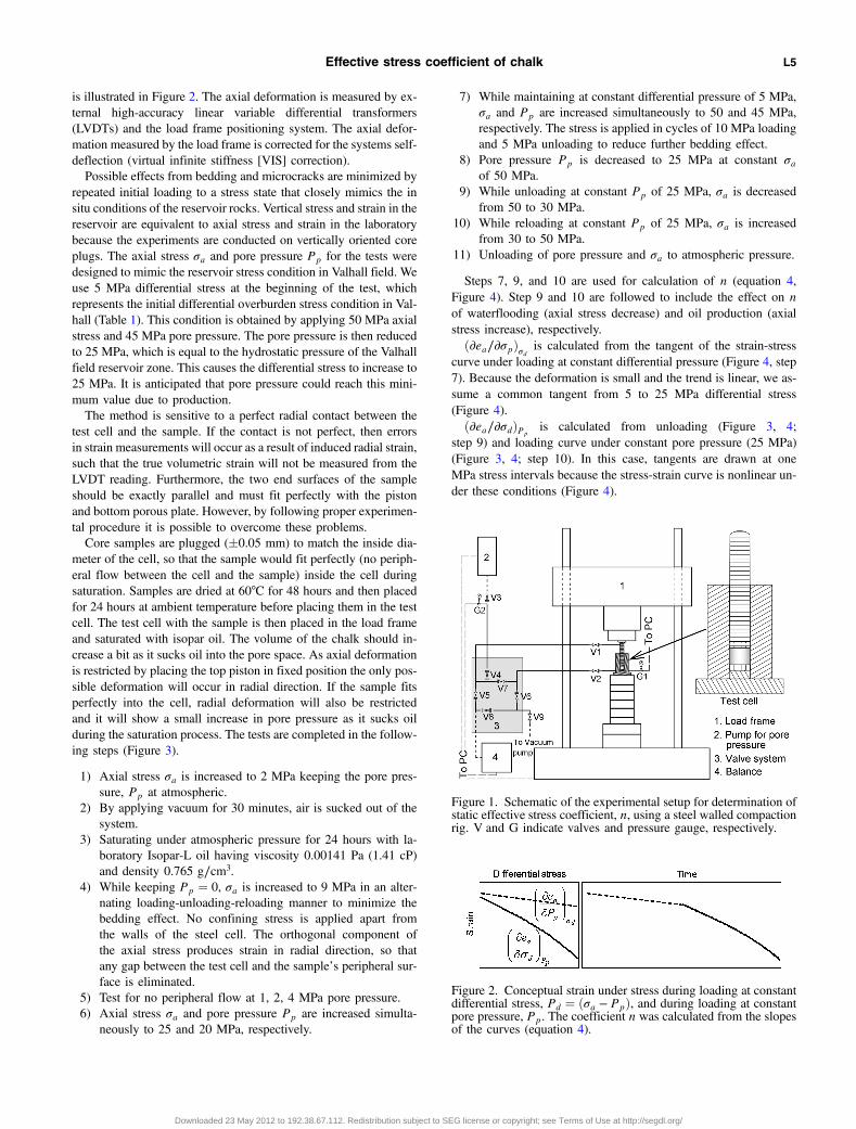
is illustrated in Figure 2. The axial deformation is measured by ex-ternal high-accuracy linear variable differential transformers(LVDTs) and the load frame positioning system. The axial defor-mation measured by the load frame is corrected for the systems self-deflection (virtual infinite stiffness [VIS] correction).Possible effects from bedding and microcracks are minimized by

repeated initial loading to a stress state that closely mimics the insitu conditions of the reservoir rocks. Vertical stress and strain in thereservoir are equivalent to axial stress and strain in the laboratorybecause the experiments are conducted on vertically oriented coreplugs. The axial stress σa and pore pressure Pp for the tests weredesigned to mimic the reservoir stress condition in Valhall field. Weuse 5 MPa differential stress at the beginning of the test, whichrepresents the initial differential overburden stress condition in Val-hall (Table 1). This condition is obtained by applying 50 MPa axialstress and 45 MPa pore pressure. The pore pressure is then reducedto 25 MPa, which is equal to the hydrostatic pressure of the Valhallfield reservoir zone. This causes the differential stress to increase to25 MPa. It is anticipated that pore pressure could reach this mini-mum value due to production.The method is sensitive to a perfect radial contact between the

test cell and the sample. If the contact is not perfect, then errorsin strain measurements will occur as a result of induced radial strain,such that the true volumetric strain will not be measured from theLVDT reading. Furthermore, the two end surfaces of the sampleshould be exactly parallel and must fit perfectly with the pistonand bottom porous plate. However, by following proper experimen-tal procedure it is possible to overcome these problems.Core samples are plugged (�0.05 mm) to match the inside dia-

meter of the cell, so that the sample would fit perfectly (no periph-eral flow between the cell and the sample) inside the cell duringsaturation. Samples are dried at 60°C for 48 hours and then placedfor 24 hours at ambient temperature before placing them in the testcell. The test cell with the sample is then placed in the load frameand saturated with isopar oil. The volume of the chalk should in-crease a bit as it sucks oil into the pore space. As axial deformationis restricted by placing the top piston in fixed position the only pos-sible deformation will occur in radial direction. If the sample fitsperfectly into the cell, radial deformation will also be restrictedand it will show a small increase in pore pressure as it sucks oilduring the saturation process. The tests are completed in the follow-ing steps (Figure 3).

1) Axial stress σa is increased to 2 MPa keeping the pore pres-sure, Pp at atmospheric.

2) By applying vacuum for 30 minutes, air is sucked out of thesystem.

3) Saturating under atmospheric pressure for 24 hours with la-boratory Isopar-L oil having viscosity 0.00141 Pa (1.41 cP)and density 0.765 g∕cm3.

4) While keeping Pp ¼ 0, σa is increased to 9 MPa in an alter-nating loading-unloading-reloading manner to minimize thebedding effect. No confining stress is applied apart fromthe walls of the steel cell. The orthogonal component ofthe axial stress produces strain in radial direction, so thatany gap between the test cell and the sample’s peripheral sur-face is eliminated.

5) Test for no peripheral flow at 1, 2, 4 MPa pore pressure.6) Axial stress σa and pore pressure Pp are increased simulta-

neously to 25 and 20 MPa, respectively.

7) While maintaining at constant differential pressure of 5 MPa,σa and Pp are increased simultaneously to 50 and 45 MPa,respectively. The stress is applied in cycles of 10 MPa loadingand 5 MPa unloading to reduce further bedding effect.

8) Pore pressure Pp is decreased to 25 MPa at constant σaof 50 MPa.

9) While unloading at constant Pp of 25 MPa, σa is decreasedfrom 50 to 30 MPa.

10) While reloading at constant Pp of 25 MPa, σa is increasedfrom 30 to 50 MPa.

11) Unloading of pore pressure and σa to atmospheric pressure.

Steps 7, 9, and 10 are used for calculation of n (equation 4,Figure 4). Step 9 and 10 are followed to include the effect on nof waterflooding (axial stress decrease) and oil production (axialstress increase), respectively.ð∂ea∕∂σpÞσd is calculated from the tangent of the strain-stress

curve under loading at constant differential pressure (Figure 4, step7). Because the deformation is small and the trend is linear, we as-sume a common tangent from 5 to 25 MPa differential stress(Figure 4).ð∂ea∕∂σdÞPp

is calculated from unloading (Figure 3, 4;step 9) and loading curve under constant pore pressure (25 MPa)(Figure 3, 4; step 10). In this case, tangents are drawn at oneMPa stress intervals because the stress-strain curve is nonlinear un-der these conditions (Figure 4).

Figure 2. Conceptual strain under stress during loading at constantdifferential stress, Pd ¼ ðσa − PpÞ, and during loading at constantpore pressure, Pp. The coefficient n was calculated from the slopesof the curves (equation 4).

Figure 1. Schematic of the experimental setup for determination ofstatic effective stress coefficient, n, using a steel walled compactionrig. V and G indicate valves and pressure gauge, respectively.

Effective stress coefficient of chalk L5

Downloaded 23 May 2012 to 192.38.67.112. Redistribution subject to SEG license or copyright; see Terms of Use at http://segdl.org/

The theory used for calculating the static effective stress coeffi-cient assumes that there is no elastic hysteresis. This is only possibleif the rock is perfectly elastic, which is rare in nature. To address thechange in elasticity, the stress gradient is measured for very small(1 MPa) stress intervals. On this scale, the hysteresis is so small thatit can be neglected.

RESULTS

Characterization

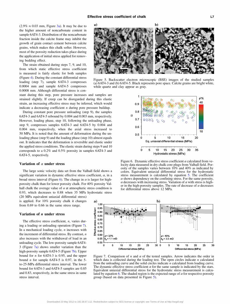
The two studied samples are notably different in porosity, perme-ability, and mineralogy (Table 2). Sample 6AT4-3 is used as a re-presentative for 30% porosity chalk and sample 6AT4-5 is used as arepresentative for 40% porosity chalk from the Valhall field. Thestudied chalk is classified as mudstone according to Dunham(1962) classification (Figure 5). Sample 6AT4-5 has fairly purecalcite mineralogy (93% CaCO3), whereas, sample 6AT4-3 con-tains a significant amount of noncarbonate (81% CaCO3). Thenoncarbonate fraction in sample 6AT4-3 comprises quartz andkaolinite. Sample 6AT4-5 contains illite in addition to quartz andkaolinite.

Deformation and porosity change in static test

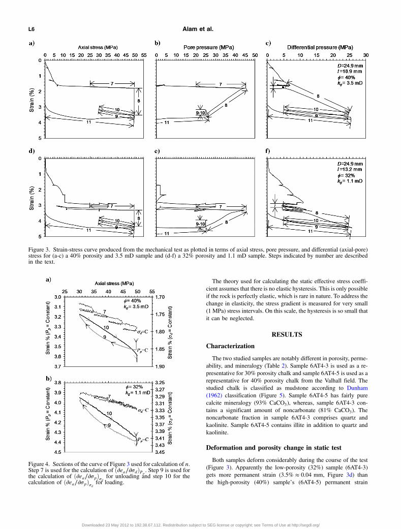
Both samples deform considerably during the course of the test(Figure 3). Apparently the low-porosity (32%) sample (6AT4-3)gets more permanent strain (3.5% ≈ 0.04 mm, Figure 3d) thanthe high-porosity (40%) sample’s (6AT4-5) permanent strain

Figure 3. Strain-stress curve produced from the mechanical test as plotted in terms of axial stress, pore pressure, and differential (axial-pore)stress for (a-c) a 40% porosity and 3.5 mD sample and (d-f) a 32% porosity and 1.1 mD sample. Steps indicated by number are describedin the text.

Figure 4. Sections of the curve of Figure 3 used for calculation of n.Step 7 is used for the calculation of ð∂ea∕∂σdÞPp

. Step 9 is used forthe calculation of ð∂ea∕∂σpÞσd for unloading and step 10 for thecalculation of ð∂ea∕∂σpÞσd for loading.

L6 Alam et al.

Downloaded 23 May 2012 to 192.38.67.112. Redistribution subject to SEG license or copyright; see Terms of Use at http://segdl.org/

(2.9% ≈ 0.03 mm, Figure 3a). It may be due tothe higher amount of noncarbonate content insample 6AT4-3. Distribution of the noncarbonatefraction inside the calcite frame may inhibit thegrowth of grain contact cement between calcitegrains, which makes this chalk softer. However,most of the porosity reduction takes place duringthe application of initial stress applied for remov-ing bedding effect.The strain obtained during steps 7, 9, and 10,

from which static effective stress coefficientis measured is fairly elastic for both samples(Figure 4). During the constant differential stressloading (step 7), sample 6AT4-3 compresses0.0004 mm and sample 6AT4-5 compresses0.0008 mm. Although differential stress is con-stant during this step, pore pressure increases and samples arestrained slightly. If creep can be disregarded during this elasticstrain, an increasing effective stress may be inferred, which wouldindicate a decreasing coefficient n during pore pressure buildup.During constant pore pressure unloading (step 9), the samples

6AT4-3 and 6AT4-5 rebound by 0.004 and 0.003 mm, respectively.However, loading phase, step 10, following the unloading phase,step 9, compresses samples 6AT4-3 and 6AT4-5 by 0.004 and0.004 mm, respectively, when the axial stress increased to50 MPa. It is noted that the amount of deformation during the un-loading phase (step 9) and the loading phase (step 10) almost equalsout. It indicates that the deformation is reversible and elastic underthe applied stress conditions. The elastic strain during steps 9 and 10corresponds to a 0.2% and 0.5% porosity in samples 6AT4-3 and6AT4-5, respectively.

Variation of α under stress

The large sonic velocity data set from the Valhall field shows asignificant variation in dynamic effective stress coefficient, α, in abroad stress interval (Figure 6). The change in α is larger for high-porosity chalk than for lower porosity chalk. For 40% porosity Val-hall chalk the average value of α at atmospheric stress condition is0.93, which decreases to 0.88 when 35 MPa hydrostatic stress(20 MPa equivalent uniaxial differential stress)is applied. For 10% porosity chalk it changesfrom 0.69 to 0.66 in the same stress range.

Variation of n under stress

The effective stress coefficient, n, varies dur-ing a loading or unloading operation (Figure 7).In a mechanical loading cycle, n increases withthe increment of differential stress. By contrast, nalso increases with the withdrawal of load in anunloading cycle. The low-porosity sample 6AT4-3 (Figure 7a) shows smaller variation than thehigh-porosity sample 6AT4-5 (Figure 7b). Upperbound for n for 6AT4-3 is 0.95, and the upperbound n for sample 6AT4-5 is 0.97, in the 5-to-25-MPa differential stress interval. The lowerbound for 6AT4-3 and 6AT4-5 samples are 0.85and 0.83, respectively, in the same stress in samestress interval.

Figure 5. Backscatter electron microscopic (BSE) images of the studied samples(a) 6AT4-3 and (b) 6AT4-5. Black represents pore space. Calcite grains are bright white,while quartz and clay appear as gray.

Figure 6. Dynamic effective stress coefficient α calculated from ve-locity data measured in dry chalk core plugs from Valhall field. Por-osity of the samples varies between 10% and 40% as indicated bycolors. Equivalent uniaxial differential stress for the hydrostaticstress measurement is calculated by equation 5. The coefficientα shows dependency on the confining stress. For the same porosity,α decreases with increasing stress. Variation of α with stress is high-er in the high-porosity samples. The rate of decrease of α decreasesfor differential stress above 12 MPa.

Figure 7. Comparison of n and α of the tested samples. Arrow indicates the order inwhich data is collected during the loading test. The open circles indicate n calculatedfrom the unloading curve and the solid circles indicate n calculated from loading curve.The dynamic effective stress coefficient α for the same sample is indicated by the stars.Equivalent uniaxial differential stress for the hydrostatic stress measurement is calcu-lated by equation 6. The shaded region is the expected range of α for respective porositygroup (based on data presented in Figure 5).

Effective stress coefficient of chalk L7

Downloaded 23 May 2012 to 192.38.67.112. Redistribution subject to SEG license or copyright; see Terms of Use at http://segdl.org/

The variations with stress of n and α for the studied samples areshown in Figure 7. We made a prediction of stress dependent α foreach porosity group from the distribution in the large data set(Figure 6) as indicated by the shaded region in Figure 7.

DISCUSSION

Behavior of α

The dynamic effective stress coefficient of chalk is in several pa-pers described as a function of porosity only (e.g., Krief et al., 1990;Engstrøm, 1992). However, this kind of relationship may not fullyrepresent the behavior of α. Our results indicate that α is not (only) aporosity-dependent coefficient. Laboratory (dynamic) measure-ments demonstrate that in the range of 20 MPa, differential stressα can vary up to 10% (Figure 6) for high-porosity reservoir chalkfrom Valhall. This observation is in accordance with Gommesenet al. (2007). They find α as a positive function of porosity withgradient defined by the cementation between grains contacts.The variation of α can be illustrated by means of effective med-

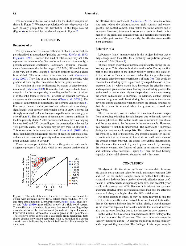
ium model (Fabricius, 2003). It indicates that it is possible to have arange in α for the same porosity depending on the fraction of miner-al in the solid frame (Figure 8). For chalk of constant porosity, αdecreases as the cementation increases (Olsen et al., 2008b). Thedegree of cementation is indicated by the isoframe values (Figure 8).For poorly cemented rocks (low isoframe value), α does not changesignificantly with porosity and remains close to unity, whereas forstrongly cemented rocks, α decreases rapidly with decreasing por-osity (Figure 8). The influence of cementation is more significant inthe low-porosity chalk. A 20% porosity chalk may have a α rangingbetween 0.60 and 0.92, depending on the cementation, whereas for40% porosity chalk, the variation may be less than 0.1 (Figure 8).This observation is in accordance with Alam et al. (2010): theyshow that during the diagenesis process of deep sea carbonate ooze,α does not decrease with porosity unless cementation between thegrain contacts starts to develop.Contact cement precipitation between the grains depends on the

diagenetic process of the chalk which in turn impacts on the value of

the effective stress coefficient (Alam et al., 2010). Presence of fineclay may reduce the calcite-to-calcite grain contacts and conse-quently, the contact cement. This makes the frame weaker and αincreases. However, increases in stress may result in elastic defor-mation of the grains and contact cement and therefore increasing thearea of the grain contact. Consequently, the effective stress coeffi-cient decreases.

Behavior of n

Laboratory (static) measurements in this project indicate that nmay change more than 10% for a probably insignificant porositychange of 0.5% (Figure 7).The test results show that n increases significantly during the un-

loading cycle. This behavior is similar to that of α. During the firstpart of the unloading of the higher porosity sample, the static ef-fective stress coefficient n has lower value than the possible rangeof dynamic effective stress coefficient α (Figure 7b). This could bebecause the unloading cycle is preceded by a rapid decrease in porepressure (step 8), which would have increased the effective stressand expanded grain contact area. During the unloading process thegrains tend to restore their original shape, thus contact area amongthe grains reduces and n increases. In addition, contact cementbetween the grains could break during this process as the cementdevelops during diagenesis when the grains are already strained, sothat the cement is strained when the grains are relaxed andvice versa.There is a sudden drop in n when the direction of stress changes

from unloading to loading. It could happen due to the rapid reversalof loading direction. The system could take some time to equilibrateand the stress state to be the same in the entire sample. However,this behavior is not fully understood. The coefficient n increasesduring the loading cycle (step 10). This behavior is opposite tothe trend of α, and is unexpected. One possible reason for this in-crease in n is that the increment of axial stress could break some ofthe contact cement between the grains (irreversible deformation).This decreases the amount of grain to grain contact. By breakingthe contact cement, the fraction of grain in suspension increasesand isoframe value decreases (Figure 8). Thus, the load bearingcapacity of the solid skeleton decreases and n increases.

CONCLUSION

The dynamic effective stress coefficient, α as calculated from so-nic data is not a constant value for chalk and ranges between 0.80and 0.95 for the studied samples from the Valhall field. Our me-chanical tests indicate that α predicts the static effective stress coef-ficient, n, well for chalk with porosity near 30%, and acceptably forchalk with porosity near 40%. Because it is evident that dynamicand static effective stress coefficients are less than one, the effectivestress will always be higher than the differential stress.For rapid change in stress, it may be more relevant to use the

effective stress coefficient n derived from mechanical tests ratherthan α. Our results indicate that for Valhall chalk, n would increaseas the reservoir depletes. Our results indicate that n could increasealso during waterflooding due to the increase in pore pressure.In the Valhall field, reservoir compaction and stress history of the

rock are monitored by 4D seismic. The stress induced changes invelocity measured during 4D seismic monitoring include porosityand compressibility alteration. The findings of this project may be

Figure 8. Theoretical bounds for effective stress coefficient to-gether with isoframe curves for a calcite (bulk modulus 75 GPa)and brine (bulk modulus 2.40 GPa) system. Reuss (1929) gives soft-est and Voigt (1910) gives stiffest bounds of a fluid-solid system.The coefficient α calculated from core data sorted according to hy-drostatic stress of the measurement (as indicated by color code).Equivalent uniaxial differential stress is given in the parenthesis.The effective stress coefficient n calculated from mechanical tests(black circles) shows good agreement with α. Variation of n duringa static test is indicated by the black bold vertical line through thedata point.

L8 Alam et al.

Downloaded 23 May 2012 to 192.38.67.112. Redistribution subject to SEG license or copyright; see Terms of Use at http://segdl.org/

used to analyze the stress induced mechanical changes in the rocksdue to pore pressure changes, which could assist in better under-standing of 4D seismic response.

ACKNOWLEDGMENTS

The financial support from BP Norway and the other Valhall part-ners (Hess, Shell, and Total) is gratefully acknowledged. The inter-pretation and conclusions in this paper is the authors and do notnecessarily represent the view of the Valhall license. Special thanksto Tron G. Kristiansen of BP Norway for providing data and sam-ples. We thank Kathrine Hedegaard and Frederik P. Ditlevsen of theDanish Geotechnical Institute (GEO) for helping with the experi-mental setup.

APPENDIX A

DERIVATION OF EFFECTIVE STRESSCOEFFICIENT UNDER UNIAXIAL STRESS

Let us consider σx, σy, and σz as the normal stress componentsparallel with the x, y, and z coordinate axes, respectively, and thecorresponding shear stress component as τx, τy, and τz. Deformationcorresponding to the stress components σx, σy, σz, τx, τy, and τz areex, ey, ez, γx, γy, and γz, respectively. Additionally, in a rock filledwith pore fluid, θ is the increment in porosity due to an increment influid pressure Pp.Let us consider a uniaxial system in compression, for which σx ¼

σy ¼ þσr and σz ¼ þσa.According to Terzaghi (1923), pore fluid pressure Pp will act in

the opposite direction of the principal stresses σx, σy, and σz, hence,deformation equations as expressed by Biot (1941, equation 2.4)become

ex ¼ −σxE

þ ν

Eðσy þ σzÞ þ

Pp

3H; (A-1a)

ey ¼ −σyE

þ ν

Eðσz þ σxÞ þ

Pp

3H; (A-1b)

ez ¼ −σzE

þ ν

Eðσx þ σyÞ þ

Pp

3H; (A-1c)

where E is the Young’s Modulus and H is a physical constant de-fined by Biot (1941) as a measure of the modulus of the rock for achange in pore pressure.Here, we consider negative sign for compression, which changes

the signs of the original derivation of Biot (1941). Biot (1941) madethe basic derivation based on tensile forces and described how to usethese equations for rocks, in which the stress is compressive, and hechanged the sign in Section 3 of his paper (Biot, 1941).The radial component of the compressive force creates tensile

stress in the axial direction. Therefore, the strain component inthe axial direction due to the radial stress has opposite (positive)sign of the strain component due to the axial stress (equation A-1).For uniaxial systems where radial deformation is constrained,

we get

ex ¼ ey ¼ er ¼ 0 and ez ¼ ea (A-2)

From equation A-1c,

ea ¼ −σaE

þ ν

Eðσr þ σrÞ þ

Pp

3H;

ea ¼ −σaE

þ ν

Eð2σrÞ þ

Pp

3H: (A-3)

From equation A-1a or equation A-1b,

σr ¼ν

ð1 − νÞ σa þ1

ð1 − νÞEPp

3H: (A-4)

Inserting value of σr from equation A-4 in equation A-3,

ea ¼ −σaE

þ 2ν

E

�ν

ð1 − νÞ σa þ1

ð1 − νÞEPp

3H

�þ Pp

3H;

σa ¼Eð1 − νÞ

ð1þ νÞð1 − 2νÞ ea þE

ð1 − 2νÞPp

3H: (A-5)

From the relationship among compressional modulus M,Young’s modulus E, shear modulus μ, and Poisson’s ratio ν:

M ¼ Eð1 − νÞð1þ νÞð1 − 2vÞ and

E ¼ 2μð1þ νÞ:

Hence equation A-5 becomes

σa ¼ Mea þ2ð1þ νÞ3ð1 − 2νÞ

μ

HPp: (A-6)

As defined by Biot (1941), 2ð1þνÞ3ð1−2νÞ

μH ¼ α is the effective stress

coefficient for 3D consolidation. This would indicate that α isthe same for 3D and confined uniaxial deformation. For uniaxialdeformation under static condition, we denote this coefficient asn, therefore

σa ¼ Mea þ nPp: (A-7)

Differentiating equation A-7 with respect to differential stresswhen pore pressure is constant

�∂ea∂σd

�Pp

¼ 1

M: (A-8a)

Differentiating equation A-7 with respect to pore pressure whendifferential stress is constant

�∂ea∂Pp

�σd

¼ 1 − nM

: (A-8b)

Effective stress coefficient of chalk L9

Downloaded 23 May 2012 to 192.38.67.112. Redistribution subject to SEG license or copyright; see Terms of Use at http://segdl.org/

From equation A-8a and equation A-8b,

n ¼ 1 −

�∂ea∂Pp

�σd�

∂ea∂σd

�Pp

: (A-9)

REFERENCES

Alam, M. M., M. K. Borre, I. L. Fabricius, K. Hedegaard, B. Røgen, Z.Hossain, and A. S. Krogsbøll, 2010, Biot’s coefficient as an indicatorof strength and porosity reduction: Calcareous sediments from KerguelenPlateau: Journal of Petroleum Science and Engineering, 70, 282–297.

Andersen, M., 1988, Predicting reservoir-condition PV compressibilityfrom hydrostatics stress laboratory data: SPE Reservoir Engineering, 3,1078–1082, doi: 10.2118/14213-PA.

Andersen, M. A., 1995, Petroleum research in North Sea chalk:RF-Rogaland Research, 174.

Andreassen, K. A., and I. L. Fabricius, 2010, Biot critical frequency appliedto description of failure and yield of highly porous chalk with differentpore fluids: Geophysics, 75, E205–E213, doi: 10.1190/1.3504188.

Banthia, B. S., M. S. King, and I. Fatt, 1965, Ultrasonic shear wave velo-cities in rocks subjected to simulated overburden pressure and internalpore pressure: Geophysics, 30, 117–121, doi: 10.1190/1.1439526.

Barkved, O. I., and T. Kristiansen, 2005, Seismic time-lapse effects andstress changes: Examples from a compacting reservoir: The LeadingEdge, 24, 1244–1248, doi: 10.1190/1.2149636.

Berryman, J. G., 1992, Effective stress for transport properties ofinhomogeneous porous rock: Journal of Geophysical Research, 97,17409–17424, doi: 10.1029/92JB01593.

Biot, M. A., 1941, General theory of three-dimensional consolidation:Journal of Applied Physics, 12, 155–164, doi: 10.1063/1.1712886.

Biot, M. A., 1956, Theory of propagation of elastic waves in a fluid-saturated porous solid. I. Low-frequency range: Journal of the AcousticalSociety of America, 28, 168–178, doi: 10.1121/1.1908239.

Carroll, M. M., and N. Katsube, 1983, The role of Terzaghi effective stress inlinearly elastic deformation: Journal of Energy Resources Technology,105, 509–511, doi: 10.1115/1.3230964.

Cheng, C. H., and D. H. Johnston, 1981, Dynamic and static moduli: Geo-physical Research Letters, 8, 39–42, doi: 10.1029/GL008i001p00039.

Christensen, N. I., and H. F. Wang, 1985, The influence of pore pressure andconfining pressure on dynamic elastic properties of Berea sandstone: Geo-physics, 50, 207–213, doi: 10.1190/1.1441910.

Ciz, R., A. F. Siggins, B. Gurevich, and J. Dvorkin, 2008, Influence of mi-croheterogeneity on effective stress law for elastic properties of rocks:Geophysics, 73, no. 1, E7–E14, doi: 10.1190/1.2816667.

Dunham, R. J., 1962, Classification of carbonate rocks according to deposi-tional texture, in W. E. Ham, ed., Classification of carbonate rocks – Asymposium: American Association of Petroleum Geologists, 1, 108–121.

Dvorkin, J., and A. Nur, 1993, Dynamic poroelasticity: A unified modelwith the squirt and the Biot mechanisms: Geophysics, 58, 524–533,doi: 10.1190/1.1443435.

Engstrøm, F., 1992, Rock mechanical properties of Danish North Sea chalk:4th North Sea Chalk Symposium.

Fabricius, I. L., 2003, How burial diagenesis of chalk sediments controlssonic velocity and porosity: AAPG Bulletin, 87, 1755–1778, doi:10.1306/06230301113.

Fabricius, I. L., 2010, A mechanism for water weakening of elastic moduliand mechanical strength of chalk: 80th Annual International Meeting,SEG, Expanded Abstracts, 2736–2740.

Fabricius, I. L., G. T. Bachle, and G. P. Eberli, 2010, Elastic moduli of dryand water-saturated carbonates: Effect of depositional texture, porosity,and permeability: Geophysics, 75, no. 3, N65–N78, doi: 10.1190/1.3374690.

Fjær, E., 2009, Static and dynamic moduli of a weak sandstone: Geophysics,74, no. 2, WA103–WA112, doi: 10.1190/1.3052113.

Frempong, P., A. Donald, and S. D. Butt, 2007, The effect of pore pressuredepletion and injection cycles on ultrasonic velocity and quality factor in aquartz sandstone: Geophysics, 72, no. 2, E43–E51, doi: 10.1190/1.2424887.

Geertsma, J., 1957, The effect of fluid pressure decline on volumetricchanges of porous rocks: Petroleum Transactions, AIME, 210, 331–340.

Gommesen, L., I. L. Fabricius, T. Mukerji, G. Mavko, and J. M. Pedersen,2007, Elastic behaviour of North Sea chalk: A well-log study: Geophy-sical Prospecting, 55, 307–322, doi: 10.1111/gpr.2007.55.issue-3.

Gurevich, B., 2004, A simple derivation of the effective stress coefficient forseismic velocities in porous rocks: Geophysics, 69, 393–397, doi:10.1190/1.1707058.

Hashin, Z., and S. Shtrikman, 1963, A variational approach to thetheory of the elastic behaviour of multiphase materials: Journal of theMechanics and Physics of Solids, 11, 127–140, doi: 10.1016/0022-5096(63)90060-7.

Hermansson, L., and J. S. Gudmundsson, 1990, Influence of production onchalk failure in the Valhall field: European Petroleum Conference.

Hornby, B. E., 1996, An experimental investigation of effective stress prin-ciples for sedimentary rocks: 66th Annual International Meeting, SEG,Expanded Abstracts, 1707–1710.

Jizba, D., and A. Nur, 1990, Static and dynamic moduli of tight gas sand-stones and their relation to formation properties: SPWLA 31st AnnualLogging Symposium.

King, M. S., 1969, Static and dynamic elasticmoduli of rocks under pressure:Proceedings of the 11th U. S. Rock Mechanics Symposium, 329–351.

Krief, M., J. Garat, J. Stellingwerff, and J. Ventre, 1990, A petrophysicalinterpretation using the velocities of P and S waves (full waveformsonic):: The Log Analyst, 31, 355–369.

Kristiansen, T., 1998, Geomechanical characterization of the overburdenabove the compacting chalk reservoir at Valhall: SPE/ISRM RockMechanics in Petroleum Engineering

Kristiansen, T., O. Barkved, K. Buer, and R. Bakke, 2005, Production-induced deformations outside the reservoir and their impact on 4Dseisimic: International Petroleum Technology Conference.

Mavko, G., and D. Jizba, 1991, Estimating grain scale fluid effects onvelocity dispersion in rocks: Geophysics, 56, 1940–1949, doi: 10.1190/1.1443005.

Mavko, G., T. Mukerji, and J. Dvorkin, 2009, The rock physics handbook:Tools for seismic analysis of porous media, 2nd ed.: Cambridge Univer-sity Press.

Mavko, G., and T. Vanorio, 2010, The influence of pore fluids and frequencyon apparent effective stress behavior of seismic velocities: Geophysics,75, no. 1, N1–N7, doi: 10.1190/1.3277251.

Montmayeur, H., and R. M. Graves, 1985, Prediction of static elastic/mechanical properties of consolidated and unconsolidated sands fromacoustic measurements: Basic measurements in SPE Annual TechnicalConference and Exhibition.

Nieto, J. A., D. P. Yale, and R. J. Evans, 1990, Core compaction correction-a different approach: Advances in core evaluation accuracy and precisionin reserves estimation: in F. Paul Worthington, ed.: Advances in CoreEvauluation: Accuracy and precision in reserves estimation: Gordonand Breach Science Publishers, 139–158.

Nur, A., and J. D. Byerlee, 1971, An exact effective stress law for elasticdeformation of rock with fluids: Journal of Geophysical Research SolidEarth, 76, 6414–6419, doi: 10.1029/JB076i026p06414.

Olsen, C., H. F. Christensen, and I. L. Fabricius, 2008a, Static and dynamicYoung’s moduli of chalk from the North Sea: Geophysics, 73, no. 2,E41–E50, doi: 10.1190/1.2821819.

Olsen, C., K. Hedegaard, I. L. Fabricius, andM. Prasad, 2008b, Prediction ofBiot’s coefficient from rock-physical modeling of North Sea chalk: Geo-physics, 73, no. 2, E89–E96, doi: 10.1190/1.2838158.

Omdal, E., H. Breivik, K. E. Næss, G. G. Ramos, T. G. Kristiansen, R. I.Korsnes, A. Hiort, and M. V. Madland, 2009, Experimental investigationof the effective stress coefficient for various high porosity outcrop chalks:43rd U.S. Rock Mechanics Symposium and 4th U.S.-Canada RockMechanics Symposium.

Plona, T. J., and J. M. Cook, 1995, Effects of stress cycles on static anddynamic Young’s moduli in Castlegate sandstone: 35th U.S. Symposiumon Rock Mechanics.

Prasad, M., and M. H. Manghnani, 1997, Effects of pore and differentialpressure on compressional wave velocity and quality factor in Bereaand Michigan sandstones: Geophysics, 62, 1163–1176, doi: 10.1190/1.1444217.

Reuss, Z. A. A., 1929, Berechnung der Fliessgrenze von Mischkristallen aufgrund der Plastizitätsbedingungen für Einkristalle: Zeitschrift für Ange-wandte Mathematik und Mechanik, 9, 49–58.

Simmons, G., and W. F. Brace, 1965, Comparison of static and dynamicmeasurements of compressibility of rocks: Journal of GeophysicalResearch, 70, 5649–5656, doi: 10.1029/JZ070i022p05649.

Teeuw, D., 1971, Prediction of formation compaction from laboratorycompressibility data: SPE Journal, 11, 263–271.

Terzaghi, K., 1923, Die Beziehungen zwischen Elastizitat und Innendruck:Sitzungsberichte, Akademie der Wissenschaften, K I. IIa 132 (3-4),105–121.

Teufel, L. W., and N. R. Warpinski, 1990, Laboratory determination ofeffective stress laws for deformation and permeability of chalk: 3rd NorthSea Chalk Symposium.

Tjetland, G., T. Kristiansen, and K. Buer, 2007, Reservoir managementaspects of early waterflood response after 25 years of depletion in theValhall field: International Petroleum Technology Conference.

Todd, T., and G. Simmons, 1972, Effect of pore pressure on thevelocity of compressional waves in low-porosity rocks: Journal of Geo-physical Research, 77, 3731–3743, doi: 10.1029/JB077i020p03731.

L10 Alam et al.

Downloaded 23 May 2012 to 192.38.67.112. Redistribution subject to SEG license or copyright; see Terms of Use at http://segdl.org/

Tutuncu, A. N., A. L. Podio, and M. M. Sharma, 1994, Strainamplitude and stress dependence of static moduli in sandstonesand limestones in P. P. Nelson, and S. E. Laubach, eds., Rock mecha-nics: Models and measurements challenges from industry: Balkema,489–496.

Tutuncu, A. N., and M. M. Sharma, 1992, Relating static and ultrasoniclaboratory measurements to acoustic log measurements in tight gas sands:SPE Annual Technical Conference and Exhibition.

Voigt, W., 1910, Lehrbuch der kristallphysik: B.G. Terebner.Wang, Z., 2000, Dynamic versus static elastic properties of reservoir rocks,in Z. Wang, and A. Nur, eds., Seismic and acoustic velocities in reservoirrocks; Volume 3: Recent developments: Geophysics Reprint Series, 19,531–539.

Yale, D. R., J. A. Nieto, and S. P. Austin, 1995, The effect of cementation onthe static and dynamic mechanical properties of the Rotliegendes sand-stone: 35th U. S. Symposium on Rock Mechanics.

Effective stress coefficient of chalk L11

Downloaded 23 May 2012 to 192.38.67.112. Redistribution subject to SEG license or copyright; see Terms of Use at http://segdl.org/