Static and Dynamic Contact Angle Measurement on Rough Surfaces UsingSessile Drop Profile Analysis with Application to Water Management in

Low Temperature Fuel Cells

By

Vinaykumar Konduru

A THESIS

Submitted in partial fulfillment of the requirements for the degree of

MASTER OF SCIENCE

(Mechanical Engineering)

MICHIGAN TECHNOLOGICAL UNIVERSITY

2010

Copyright © 2010 Vinaykumar Konduru

This thesis, “Static and Dynamic Contact Angle Measurement on Rough SurfacesUsing Sessile Drop Profile Analysis with Application to Water Management in LowTemperature Fuel Cells,” is hereby approved in partial fulfillment for the requirementsfor the Degree of MASTER OF SCIENCE IN Mechanical Engineering.

Department of Mechanical Engineering – Engineering Mechanics

Advisor:Dr. Jeffrey S. Allen

Committee Member:Dr. Jaroslaw Drelich

Committee Member:Dr. Chang Kyoung Choi

Department Chair:Professor William W. Predebon

Date:

Abstract

Fuel Cells are a promising alternative energy technology. One of the biggest problemsthat exists in fuel cell is that of water management. A better understanding ofwettability characteristics in the fuel cells is needed to alleviate the problem of watermanagement. Contact angle data on gas diffusion layers (GDL) of the fuel cellscan be used to characterize the wettability of GDL in fuel cells. A contact anglemeasurement program has been developed to measure the contact angle of sessiledrops from drop images. Digitization of drop images induces pixel errors in the contactangle measurement process. The resulting uncertainty in contact angle measurementhas been analyzed. An experimental apparatus has been developed for contact anglemeasurements at different temperature, with the feature to measure advancing andreceding contact angles on gas diffusion layers of fuel cells.

Acknowledgments

I owe my deepest gratitude to my advisor Dr. Jeffrey Allen for whose continuoussupport, patience and guidance enabled me in all time of research and writing thisthesis. I would also like to thank the entire MNiT research group and Chelsey Smithin particular for the help she provided in collecting the data for my work.

Contents

Abstract iii

Acknowledgments iv

Table of Contents vi

List of Figures viii

List of Tables ix

1 Introduction 11.1 Techniques for Measuring Contact Angle . . . . . . . . . . . . . . . . 3

1.1.1 Wilhelmy Plate Method . . . . . . . . . . . . . . . . . . . . . 31.1.2 Goniometry . . . . . . . . . . . . . . . . . . . . . . . . . . . . 4

1.2 Contact Angle on Rough Surfaces . . . . . . . . . . . . . . . . . . . . 5

2 Sessile Drop Profile Analysis 72.1 Numerical Optimization . . . . . . . . . . . . . . . . . . . . . . . . . 102.2 Code Verification . . . . . . . . . . . . . . . . . . . . . . . . . . . . . 13

3 Accuracy in Contact Angle Measurement 143.1 Drop edge detection . . . . . . . . . . . . . . . . . . . . . . . . . . . 143.2 Edge Detection Accuracy . . . . . . . . . . . . . . . . . . . . . . . . . 163.3 Uncertainty in Exact Scale Calculation . . . . . . . . . . . . . . . . . 183.4 Illumination Control . . . . . . . . . . . . . . . . . . . . . . . . . . . 193.5 Solid-Liquid Interface Detection . . . . . . . . . . . . . . . . . . . . . 19

4 Experimental Procedure 234.1 Experimental Setup . . . . . . . . . . . . . . . . . . . . . . . . . . . . 234.2 Static Measurement . . . . . . . . . . . . . . . . . . . . . . . . . . . . 254.3 Dynamic Contact Angle Measurement . . . . . . . . . . . . . . . . . 254.4 Humidity Control . . . . . . . . . . . . . . . . . . . . . . . . . . . . . 25

v

5 Results 265.1 Asymmetry in Drop Profile . . . . . . . . . . . . . . . . . . . . . . . 275.2 Static Contact Angle Data . . . . . . . . . . . . . . . . . . . . . . . . 295.3 Dynamic Contact Angle on GDL . . . . . . . . . . . . . . . . . . . . 30

6 Conclusion 366.1 Summary . . . . . . . . . . . . . . . . . . . . . . . . . . . . . . . . . 366.2 Recommendations . . . . . . . . . . . . . . . . . . . . . . . . . . . . . 37

Appendices 38

A Abbreviations 39

B Contact Angle Measurement Programs 412.1 scale . . . . . . . . . . . . . . . . . . . . . . . . . . . . . . . . . . . . 412.2 needle_Scale . . . . . . . . . . . . . . . . . . . . . . . . . . . . . . . 452.3 Contact Angle Measurement Program . . . . . . . . . . . . . . . . . . 472.4 Functions . . . . . . . . . . . . . . . . . . . . . . . . . . . . . . . . . 56

2.4.1 abs_data_pts . . . . . . . . . . . . . . . . . . . . . . . . . . . 562.4.2 bc_optimization . . . . . . . . . . . . . . . . . . . . . . . . . 572.4.3 bc_optimization_la . . . . . . . . . . . . . . . . . . . . . . . 592.4.4 cfinder . . . . . . . . . . . . . . . . . . . . . . . . . . . . . . . 612.4.5 cfinder_la . . . . . . . . . . . . . . . . . . . . . . . . . . . . . 632.4.6 contact_angle . . . . . . . . . . . . . . . . . . . . . . . . . . . 652.4.7 drop_properties . . . . . . . . . . . . . . . . . . . . . . . . . . 662.4.8 edge_detector . . . . . . . . . . . . . . . . . . . . . . . . . . . 662.4.9 error . . . . . . . . . . . . . . . . . . . . . . . . . . . . . . . . 672.4.10 exact_data . . . . . . . . . . . . . . . . . . . . . . . . . . . . 682.4.11 image_analysis . . . . . . . . . . . . . . . . . . . . . . . . . . 692.4.12 image_input . . . . . . . . . . . . . . . . . . . . . . . . . . . 702.4.13 initial_guess . . . . . . . . . . . . . . . . . . . . . . . . . . . 712.4.14 laplace . . . . . . . . . . . . . . . . . . . . . . . . . . . . . . . 732.4.15 plane . . . . . . . . . . . . . . . . . . . . . . . . . . . . . . . . 742.4.16 pixel_data . . . . . . . . . . . . . . . . . . . . . . . . . . . . . 762.4.17 profile_split . . . . . . . . . . . . . . . . . . . . . . . . . . . . 792.4.18 scale_data . . . . . . . . . . . . . . . . . . . . . . . . . . . . . 792.4.19 volume . . . . . . . . . . . . . . . . . . . . . . . . . . . . . . . 80

2.5 images_reader . . . . . . . . . . . . . . . . . . . . . . . . . . . . . . . 812.6 Data_modifier . . . . . . . . . . . . . . . . . . . . . . . . . . . . . . 83

vi

List of Figures

1.1 PEM Fuel Cell Assembly . . . . . . . . . . . . . . . . . . . . . . . . . 11.2 Young’s Model of Sessile Drop . . . . . . . . . . . . . . . . . . . . . . 31.3 Contact angle measurement using Wilhelmy Plate method . . . . . . 41.4 Wetting on Rough Surfaces . . . . . . . . . . . . . . . . . . . . . . . 5

2.1 Variation in drop shape with respect to B . . . . . . . . . . . . . . . 92.2 Variation in drop shape with respect to c (cm−2) at constant B = 0.4 102.3 Calculation of error over the drop profile. (offsets are exagerrated) . . 112.4 Variation of error vs capillary constant . . . . . . . . . . . . . . . . . 112.5 Error Optimization . . . . . . . . . . . . . . . . . . . . . . . . . . . . 122.6 Error Optimization . . . . . . . . . . . . . . . . . . . . . . . . . . . . 12

3.1 Drop Edge Detection (GDL: Toray T060,9%PTFE(wt)) . . . . . . . . 143.2 Edge Detection Approximation . . . . . . . . . . . . . . . . . . . . . 153.3 Change in pixel intensity along normal to drop profile . . . . . . . . . 163.4 Distribution of ∆θ between Position 3 and Positions 1, 2, 4 and 5 . . 173.5 Error in Contact Angle Measurements with Error in Scale Calculation 183.6 Error in θ with Solid-Liquid Interface (Scale = 2µm/pixel) . . . . . . 203.7 Error in θ with Solid-Liquid Interface (Scale = 2µm/pixel) . . . . . . 213.8 Error in θ with Solid-Liquid Interface (Scale = 5µm/pixel) . . . . . . 22

4.1 Schematic Diagram of experimental setup for ADSA . . . . . . . . . . 234.2 Image of the stage with enclosure . . . . . . . . . . . . . . . . . . . . 244.3 Setup for liquid infusion and withdrawl . . . . . . . . . . . . . . . . . 24

5.1 SEM images of GDL samples tested for contact angle measurement . 275.2 Difference in θ between left and right side of drop . . . . . . . . . . . 285.3 Static Contact Angle on Baseline vs temperature . . . . . . . . . . . 295.4 Advancing Contact Angle on Toray obtained for 3 test runs at 25° C . 305.5 Advancing Contact Angle on Mitsubishi vs temperature . . . . . . . . 315.6 Receding Contact Angle on Mitsubishi vs temperature . . . . . . . . 315.7 Advancing Contact Angle on SGL vs temperature . . . . . . . . . . . 32

vii

5.8 Receding Contact Angle on SGL vs temperature . . . . . . . . . . . . 325.9 Advancing Contact Angle on Freudenberg vs temperature . . . . . . . 335.10 Receding Contact Angle on Freudenberg vs temperature . . . . . . . 335.11 Advancing Contact Angle on Toray vs temperature . . . . . . . . . . 345.12 Receding Contact Angle on Toray vs temperature . . . . . . . . . . . 345.13 Receding Contact Angle on Mitsubishi . . . . . . . . . . . . . . . . . 35

viii

List of Tables

2.1 Comparision of data points . . . . . . . . . . . . . . . . . . . . . . . . 92.2 Code Verification for θ = 160 ◦; c = 13.45 cm−2 . . . . . . . . . . . . 13

3.1 Samples used for pixel error estimation . . . . . . . . . . . . . . . . . 183.2 Variation of Contact Angle with Edge Detection . . . . . . . . . . . . 183.3 Variation of Contact Angle with Edge Detection . . . . . . . . . . . . 19

5.1 GDL samples tested . . . . . . . . . . . . . . . . . . . . . . . . . . . 265.2 Pore size distribution of the tested GDL samples . . . . . . . . . . . . 265.3 Difference in Contact Angle for Left and Right Side of Drop . . . . . 285.4 Mean static contact angle on GDLs at different temperatures . . . . . 30

ix

Chapter 1. Introduction

In a proton exchange membrane (PEM) fuel cell, hydrogen and oxygen react to formelectricity, water and heat. The basic assembly of a PEM fuel cell consists of polymerelectrolyte membrane which is sandwiched between two electrodes. These electrodeswhich are called gas diffusion layers (GDL) are made up of carbon cloth or carbon pa-per. A catalyst layer is bonded to the polymer membrane. This catalyst layer helps inaccelerating the rate of reactions. The GDL is coated with poly(tetrafluoroethylene)(PTFE) to make the surface hydrophobic. This aides in the removal of water to thesurface of GDL. Such an arrangement of GDLs with a polymer electrolyte membranewith catalyst forms a single fuel cell and is commonly called as membrane electrodeassembly (MEA). Different cells are connected together by means of bipolar plates.The bipolar plates have channels built into them that carry the reactants to the fuelcell and also collect the water produced in the fuel cell (Figure 1.1).

e

e e

eHydrogen Oxygen

Anode Cathode

Polymer Electrolyte

Membrane

Bipolar

Plate

H

Figure 1.1. PEM Fuel Cell Assembly

1

During operation, hydrogen in passed over anode and oxygen over cathode. Atanode, hydrogen gas dissociates producing protons and electrons. Protons travelthrough the electrolyte membrane while electrons travel through the circuit. Atcathode, they react with oxygen to form water. These reactions are given in Equations(1.1)-(1.3).

At Anode: H2 = 2H+ + 2e− (1.1)

At Cathode: O2 + 4H+ + 4e− = 2H2O (1.2)

Net cell Reaction: 2H2 +O2 = 2H2O (1.3)

Water management in a fuel cell plays a vital role for the optimal performance ofa fuel cell. Water that is formed at cathode during the fuel cell operation is removedby the reactant flow. The membrane is kept hydrated as the proton conductivityincreases with water content. If excess water is withdrawn, the membrane will dryout and thereby increasing the resistance to the motion of protons reducing the fuelcell performance. If the water removal rate is slow, the excess water that is producedforms plugs in the channels and thereby blocking the path of reactant gases andreducing the number of available reaction sites severely hampering fuel cell operation[Larminie and Dicks, 2003].

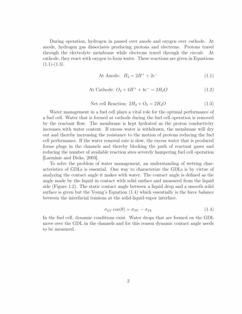
To solve the problem of water management, an understanding of wetting char-acteristics of GDLs is essential. One way to characterize the GDLs is by virtue ofanalyzing the contact angle it makes with water. The contact angle is defined as theangle made by the liquid in contact with solid surface and measured from the liquidside (Figure 1.2). The static contact angle between a liquid drop and a smooth solidsurface is given but the Young’s Equation (1.4) which essentially is the force balancebetween the interfacial tensions at the solid-liquid-vapor interface.

σLV cos(θ) = σSV − σSL (1.4)

In the fuel cell, dynamic conditions exist. Water drops that are formed on the GDLmove over the GDL in the channels and for this reason dynamic contact angle needsto be measured.

2

σLV

σSV

σSLSolid

Vapor

Fluid

Figure 1.2. Young’s Model of Sessile Drop showing relationship between InterfacialTensions

1.1 Techniques for Measuring Contact Angle

Several techniques exist to determine the contact angle, principal among thembeing the Wilhelmy Plate method and goniometry.

1.1.1 Wilhelmy Plate Method

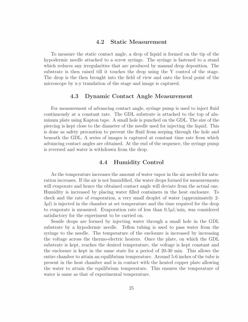
This technique can be used to measure the contact angle if the surface tension ofthe liquid is known. Similarly, if the contact angle for the given solid-liquid pair isknown, surface tension of the liquid can be obtained with this method. Wilhelmy platemethod essentially consists of a rectangular plate on which angle is to be measuredand a reservoir of the fluid kept below the plate. To measure the contact angle, thefluid is raised towards the plate until it touches the plate (Figure 1.3). The changein the weight of the plate (∆W ) occurs because of the liquid adhering to the plate.This change in weight is measured and with the knowledge of the wetted perimeter(p), the contact angle (θ) is measured from Equation 1.5.

σ cos(θ) =∆W

p(1.5)

This method of measuring the contact angle is not suitable for rough and poroussubstrates such as GDLs. The fibrous surface of a GDL coupled with pores makes itdifficult to measure the perimeter and may also result in wicking of the fluid into theGDL which result in incorrect weight measurements producing incorrect contact angleresults. A modification of the Wilhelmy plate method is the Single Fiber Wilhelmymethod in which the plate is replaced by a single fiber of the substrate. The singlefiber however is not an accurate representation of the actual GDL surface.

3

Wilhelmy

Plate

Fluid

Figure 1.3. Contact angle measurement using Wilhelmy Plate method

1.1.2 Goniometry

In goniometry, an image of the drop is obtained and contact angle is measured fromthe drop image. An elementary method is to draw a tangent and the solid-liquidinterface along the drop profile and measure the contact angle. This method is verycrude and the obtained angle is dependent on the judgement of the user and hencethis method is not suitable for scientific applications.

For very small drops with Bond number (Bo) less than 1, spherical cap approxi-mation can be applied in which the drop shape is approximated to that of a sphereby neglecting the effects of gravity. This approximation fails if the Bond numberbecomes greater than 1 as the effects of gravity cannot be neglected. The small slopeapproach [Allen, 2003] presents a simple model to obtain contact angles which areless than 30° but can be applied to drops of any size.

(

1

R1

+1

R2

)

σ = ∆P (1.6)

Contact angle measurement by fitting a curve to the drop edge gets rid of the sizeconstraints imposed by previous methods. Multiple points on the drop edge are se-lected from the images and a B-spline [Stalder et al., 2006] or any other curve is fittedto these profile points. Another approach is to model the drops using the Laplace-Young equation (1.6). A numerical solution to this equation was first developed byBashforth and Adams [1883]. Hartland and Hartley [1976] solved the Laplace-Youngequation numerically using the fourth order Runge-Kutta method and obtained theexact drop profile for different drop parameters. Cheng et al. [1990] followed a sim-

4

ilar approach and developed a technique called Axisymmetric Drop Shape Analysis(ADSA), to fit the obtained theoretical drop profiles to the drop edge obtained fromthe images.

Young’s equation (1.4) is applicable to systems with smooth and homogeneoussurfaces only. On rough and heterogenous surfaces as found on GDLs, contact anglesobtained using Young’s correlation would be incorrect. Modifications to the Young’sequation have been established previously and will be discussed in Section 1.2

1.2 Contact Angle on Rough Surfaces

w

(a) Wenzel

c

(b) Cassie-Baxter

Figure 1.4. Wetting on Rough Surfaces

A drop of liquid on a rough surface can take either of the two forms a) Totalwetting (Figure 1.4a), where the liquid wets the entire rough surface; or b) Partialwetting (Figure 1.4b), where vapor is trapped between the liquid and the troughs ofthe rough surface. For the case of total wetting, Wenzel [1936] developed Equation1.7 to model the apparent contact angle (θW ) on rough surfaces. Roughness factor (r)is the ratio of the true surface area and the projected surface area. For non-wettingsurfaces (θ > 90°), an increase in roughness would increase the apparent contactangle and for wetting surfaces (θ < 90°), increased surface roughness woud reduce theapparent contact angle.

cos(θW ) = r cos(θY ) (1.7)

Cassie and Baxter [1944] developed Equation 1.8 to model contact angle on het-erogenous surfaces, where fi is the fraction area of each surface under the liquid andθYi

is the contact angle for the same surface. For the case of partial wetting withvapor trapped between the solid and liquid, 1.8 takes the form of Equation 1.9, wheref1 is the fractional area for the solid-liquid interface and f2 is the fractional area forthe pores.

cos(θC) =∑

fi cos(θYi) (1.8)

5

cos(θC) = f1 cos(θY )− f2 (1.9)

The Wenzel 1.7 and Cassie-Baxter 1.9 do not consider the irregularities that occurat the solid-liquid-vapor contact line. Several modifications to these equations havebeen published. Drelich and Miller [1993], have suggested modifications to the aboveequations for different configurations of the surface at the contact line. However, dueto the lack of a uniform surface on a GDL, these equations are not applicable onGDLs.

6

Chapter 2. Sessile Drop Profile

Analysis

The Laplace equation of capillarity is the mathematical balance between the surfacetension forces and gravitational forces, for two fluids separated by an interface.

(

1

R1

+1

R2

)

σ = ∆P (2.1)

where σ is the interfacial tension, ∆ P is the pressure difference across the interface,R1 and R2 are the two principal radii at the apex. The pressure difference consists oftwo components, the hydrostatic pressure (Pg) and the pressure due to the curvature(Pσ). These are expressed as

∆Pg = ρgz (2.2)

∆Pσ =2σ

b(2.3)

Thus for any sessile drop, at a height of z from apex, the Laplace equation can beexpressed as

(

1

R1

+1

R2

)

σ =2σ

b+ ρgz (2.4)

At apex of the drop, due to symmetry of an axisymmetric drop, R1 = R2 = b

where b is the radius of curvature at the apex. The two radii of curvature can beexpressed in terms of the arc length and the angle of the tangent to the interface byrecognizing that

1

R1

=dθ

ds(2.5)

1

R2

=sin(θ)

x(2.6)

7

Equation (2.4) is then expressed as

dθ

ds=

2

b+

ρgz

σ−

sin(θ)

x(2.7)

To solve equation (2.7), it is non-dimensionalized using the capillary constant,c, which is the ratio of physical properties of the fluid, namely the density, surfacetension and gravity and has the dimensions of 1/length2.

c =ρg

σ(2.8)

The non-dimensionalized parameters that are needed to define the drop profile are

X = xc1

2 (2.9)

Z = zc1

2 (2.10)

B = bc1

2 (2.11)

S = sc1

2 (2.12)

In non-dimensionalized form, equation (2.7) is expressed as

dθ

dS=

2

B+ Z −

sin(θ)

X(2.13)

Equation (2.13) with the geometric definitions, equations (2.14) and (2.15) forma set of first order differential equations which are solved numerically to obtain therequired drop profile.

dX

dS= cos(θ) (2.14)

dZ

dS= sin(θ) (2.15)

In order to solve the above set of equations, different solvers exist in MATLAB®.The ode45 solver, which utlizes the Runge-Kutta method, was selected to obtain thedrop profile. To validate the obtained profile, a comparison is made between the pro-file obtained from ode45 and the numerical data published by Hartland and Hartley[1976]. Data points at θ = 90° are selected for comparision (Table 2.1). The obtainedprofile points are accurate and deviate only in the fourth digit, which enables us toconclude that an accurate drop profile is generated.

8

Table 2.1. Comparision of data points with numerical data published byHartland and Hartley [1976]

BHartland and Hartley ODE45

X90 Z90 X90 Z90-1.50 .0316175 .0316102 0.031627 0.031658-1.25 .0562045 .0561636 0.056224 0.056221-1.00 .0998342 .0996054 0.099872 0.099588-0.75 .176906 .175646 0.176973 0.175620-0.50 .311216 .304568 0.311345 0.304596-0.25 .536715 .505309 0.537020 0.5054500.00 .885291 .766710 0.885116 0.7669080.25 1.35895 1.02957 1.359368 1.0295980.50 1.92291 1.23563 1.923322 1.2357020.75 2.53445 1.370590 2.534496 1.3706681.00 3.16457 1.44869 3.164281 1.448872

−0.8 −0.6 −0.4 −0.2 0 0.2 0.4 0.6 0.8

−0.1

0

0.1

0.2

0.3

0.4

0.5

0.6

0.7

X−Direction

Z−

Dire

ctio

n

0.05

0.1

0.15

0.25

0.35

0.5

0.751

1.52

Figure 2.1. Variation in drop shape with respect to dimensionless radius of curvatureat apex, B

To generate a drop profile in non-dimensional co-ordinates, value of only the de-pendent variable B is needed. Figure 2.1 shows the drop profiles that are obtained fordifferent values of B. The drop profiles are dimensionalised by dividing them with c1/2.The capillary constant thus acts as a scaling factor for the generated drop profiles.Figure 2.2 shows drops generated with same B but at different values of capillaryconstant.

9

−1.5 −1 −0.5 0 0.5 1 1.5

0

0.2

0.4

0.6

0.8

1

1.2

1.4

1.6

1.8

X−Direction

Z−

Dire

ctio

n

2015

105

25

30

Figure 2.2. Variation in drop shape with respect to c (cm−2) at constant B = 0.4

2.1 Numerical Optimization

The error between the Laplacian curve and the drop profile is defined as the sumof the normal distance between the drop profile and the Laplacian curve. By applyingsuitable edge detection techniques described in Section 3.1 the drop edge is obtained.On this edge, co-ordinates of N number of points are obtained (Figure 2.3). Tocalculate the error between the Laplacian curve and the actual profile, a normal isdrawn from the N points onto the estimated Laplacian curve. The length of thenormal gives the magnitude of error at that point. The total error is the sum ofmagnitude of distances calculated for all points. The distance is positive if the datapoint on the drop lies on one side of the the Laplacian curve and negative if it lies onthe other side.

If B is kept constant and only fluid properties are changed by varying c, the errorobtained for a given drop is minimum only for one value of c. This c would then bethe optimal capillary constant corresponding to that value of B. The error obtainedfor this B-c pair would be the absolute minimum error that exists for B. Thus fordifferent values of B, the error is obtained and the one that yields minimum errorgives the solution from which contact angle is determined. Following is the procedurethat is utilized to obtain accurate drop profiles:

1. Guess the initial value of B, which is close to the actual value. The programInitial guess performs this function and utilizes the algorithm developed byStacey [2009].

2. Five values of B, two on each side of the initial guess, are selected. Obtain

10

i1

i2

i3

iN−2

iN−1

iN

X

Z

θ

Figure 2.3. Calculation of error over the drop profile. (offsets are exagerrated)

the capillary constant for each that results in minimum error by employing thebisection method (Figure 2.4).

3. Out of these five, the value that yields minimum error and adjacent two values

8 10 12 14 16 18 200

0.2

0.4

0.6

0.8

1

1.2

1.4

Capillary constant, c (cm−2

)

Err

or

betw

een D

rop (

B =

1.4

67)

and L

apla

cia

n c

urv

e

B = 1.267

B = 1.467

B = 1.667

Figure 2.4. Variation of error vs capillary constant at same non-dimensionalized radiusof curvature at apex, B. Actual drop B = 1.467, c = 13.45 (cm−2)

11

are retained and the other two values are discarded. The span between theremaining three values is divided equally to obtain 2 more values of B wherethe error is calculated again. This procedure is repeated till the limit of errorin B is within ±5e−5 (Figure 2.5 and 2.6). Typically 10 iterations are requiredto achieve this accuracy.

1.35 1.4 1.45 1.5 1.55 1.60

0.005

0.01

0.015

0.02

0.025

0.03

B

Cu

mu

lative

Err

or

1

2

3

4

5

6

7

Initial Guess

New Points

Figure 2.5. Error optimization (First iteration). (True B = 1.467, c = 13.45 cm−2)Points 1-5: Error at initial values of B. Points 1 and 5: Discarded after step 1.Points 6 and 7: New guessed values.

1.43 1.44 1.45 1.46 1.47 1.48 1.49 1.50

1

2

3

4

5

6

7

8x 10

−3

B

Cu

mu

lative

Err

or

2

6

3

7

4

8

9 Previous Iteration

New Points

Figure 2.6. Error optimization (Second iteration). (True B = 1.467, c = 13.45 cm−2)Points 2 and 4: Discarded after step 2. Points 8 and 9: New guessed values.

12

Figure 2.5 shows the results from the first iteration. Circles (points 1-5) representthe initially guessed values while the squares (points 6-7) represent the new valuesfor the next iteration. (Figure 2.6) shows the results from second iteration. Circlesrepresent data from previous iteration while the squares represent new data points.Comparing the two figures, it is seen that the error in the drop profile reduces foreach iteration.

2.2 Code Verification

To test the accuracy with which the code determines the contact angle, a dropprofile was generated using the Laplace-Young equation. Twenty one points selectedfrom this profile and the co-ordinates of these points were supplied to the program.The program can be said to operate accurately if the obtained values of b, c and thecontact angle are the same as those that were used to generate the profile. Cheng et al.[1990] discusses the effect of the number of points used for edge detection on theresultant contact angle. Significant improvement in accuracy was not seen whenmore points were selected. Table 2.2 shows the obtained values of b and c andthe actual values. Also the corresponding theta that is obtained from the program isshown. The test validates that for a given drop profile the program yields an accuratecontact angle. It also shows that twenty one points are sufficent for contact anglecalculation. However, selection of more points would result in a better estimation ofthe drop edge [Neumann and Spelt, 1996] at the expense of computational time.

Table 2.2. Code Verification for θ = 160 ◦; c = 13.45 cm−2

Actual Obtainedb c b θ

0.15 13.4506 0.1500 159.940.20 13.4502 0.2000 159.990.25 13.4497 0.2500 159.980.30 13.4504 0.3000 159.990.35 13.4501 0.3500 159.990.40 13.4500 0.4000 160.000.45 13.4497 0.4500 159.990.50 13.4502 0.5000 159.990.75 13.4501 0.7500 159.991.00 13.4499 1.0000 159.991.50 13.4500 1.5000 159.992.00 13.4500 2.0000 159.99

13

Chapter 3. Accuracy in Contact Angle

Measurement

The accuracy in contact angle measurement depends upon the image processing tech-nique that is applied for extracting the drop edge from the sessile drop images. Thischapter explains in details the effect of inaccuracies in edge detection on contact anglemeasurement.

3.1 Drop edge detection

(a) Sessile Drop

Region of Interest

(b) Gray-scale Image

(c) Pixelation in Gray-Scale Image

Figure 3.1. Drop Edge Detection (GDL: Toray T060,9%PTFE(wt))

The drop image (Figure 3.1a) is converted into a gray-scale image (Figure 3.1b)by thresholding. The gray-scale image consists of a dark foreground representing the

14

drop and a white background. The edge of the drop, however, is not accurate as itconsists of step changes in the profile (Figure 3.1c). An actual drop profile is expectedto be smooth and continuous. In addition, the obtained profile would depend on thevalue set for thresholding. To obtain the accurate drop edge [Cheng et al., 1990],intensities of pixels along a normal across the drop edge are found (Figure 3.2).The pixel intensities for 11 pixels along with a cubic spline fit is shown in Figure3.3. From the figure, we see a sharp drop in pixel intensity as we move from thebackground into the drop. The edge of the drop is expected to be in a region alongthe spline where the gradient is high. From Figure 3.3, it is evident that there lies anuncertainty in exact edge detection and the edge is therefore approximated to lie inthe region of 2-3 pixels along the normal. The effect of this uncertainty on contactangle measurements in explained in detail in Section 3.2. This procedure of findingthe edge along the normal is repeated over the entire drop profile. To further increasethe accuracy by eliminating the step changes that occur at the edge, a second-orderleast square polynomial is fitted to 11 adjacent points along the edge, and the dropedge is obtained from these polynomials.

Normal

Position 1

Position 2

Position 3

Position 4

Position 5

Figure 3.2. Edge Detection Approximation

15

1 2 3 4 5 6 7 8 9 10 110

50

100

150

200

250

300

Pixels Normal to Drop Edge

Pix

el In

tensity

Position 1

Position 2

Position 3

Position 4

Position 5

Figure 3.3. Change in pixel intensity along normal to drop profile. Pixel intensitiesfor Figure 3.2.

3.2 Edge Detection Accuracy

The uncertainty that exists in drop edge detection causes the obtained contactangles to become a function of the methodology that is used for edge detection. Theedge, can be defined to lie anywhere along spline with a high gradient (Figure 3.3). Toanalyze this effect, the region along the spline with steep pixel intensity gradient wasselected. The lower limit was obtained by averaging the pixel intensity for the darkest4 pixels (Pixels 1-4 in Figure 3.3). This limit corresponds to the lowest illuminationintensity where the drop can be located. A similar upper limt was set by the 4 brighestpixels (pixels 8-11 in Figure 3.3). However, from Figure 3.3, it is seen that there exists5 pixels (7-11) that have the intensity of 255 and hence the resulting average of the4 pixels would also be 255. To eliminate the possibility of an error that could occurwhen this average intensity is 255, the maximum value upper limit is set at 253. Theresulting difference in drop edge co-ordinates as well as the contact angle was foundto be miniscule and hence this approximation is considered valid. For situations whenthe average of the 4 brightest pixels is different from 255, the obtained average is setas the upper limit. Three more equally spaced locations were selected in the regionbetween the upper and lower limits. Figure 3.2 shows the drop edge that is obtainedfor each approximation. The drop edge obtained by each method would move deeperinto the drop as the pixel intensity level is lowered in the algorithm. For this reason,edge obtained by the approximation corresponding to Position 5 is not appropriatefor accurate contact angle determination, but is considered in the analysis.

16

−3 −2 −1 0 1 2 3 4 50

20

40

60

80

100

Difference in θ

Co

un

ts

(a) Position 1

−1 −0.5 0 0.5 10

10

20

30

40

50

Difference in θ

Co

un

ts

(b) Position 2

−2 −1 0 1 20

20

40

60

80

Difference in θ

Co

un

ts

(c) Position 3

−8 −6 −4 −2 0 2 4 6 80

20

40

60

80

Difference in θC

ou

nts

(d) Position 4

Figure 3.4. Distribution of ∆θ between Position 3 and Positions 1, 2, 4 and 5 forsamples in Table 3.1

Different sessile drop images with contact angle varying from 30° to 160° wereselected and were processed with these approximations for edge detection and thecorresponding contact angle for each method was obtained. Table 3.1 gives detailsof the samples used to obtain the images for this analysis. Figure 3.4 shows thedistribution of error in contact angle that is obtained for positions 1, 2, 4 and 5 whencompared with the contact angle obtained for Position 3. Table 3.2 summarizes thestatistical parameters of the error in contact angle measurements. An explanation forthis change in contact angle can be attributed to the change in the drop profile shapethat occurs as different edge detection schemes are implemented. For the purposeof edge calculation, data points corresponding to Position 3, i.e. midway betweenthe upper and lower limits, are selected following an analogy similar to Cheng et al.[1990].

17

Table 3.1. Samples used for pixel error estimation

Substrate Fluid Average obtained θ

Plexiglass 80% Tripropylene Glycol - 20% Water 38°±2Plexiglass 40% Tripropylene Glycol - 60% Water 57.5°±1.8Plexiglass 20% Tripropylene Glycol - 80% Water 67.5°±5.5

RainX Water 100°±3EGC1720 Water 109°±5

Toray Water 158°±3

Table 3.2. Variation of Contact Angle with Edge Detection for samples in Table 3.1

Mean Error Standard Deviation95% Region of Certaintylower limit Upper limit

Position 1 0.21 0.65 -0.86 1.28Position 2 0.05 0.26 -0.38 0.48Position 4 -0.11 0.55 -1.01 0.79Position 5 -0.05 2.13 -3.33 3.45

3.3 Uncertainty in Exact Scale Calculation

The program Scale calculates the scale by analyzing the images of the stage mi-crometer. The program accounts for any vertical mis-alignments of the micrometer.However, pixelation of image creates an inherent error in scale calculation and theerror is of the order ±1 pixel. To test the effect of this error on contact angle mea-surements, drop images with different contact angles were analysed by inducing errorin the obtained scale. Error of ±1, ±2 pixels per millimeter was induced in the scalecalculation and the results were compared with actual calculated scale.

−0.16 −0.12 −0.08 −0.04 0 0.04 0.08 0.12 0.160

20

40

60

80

Error in θ for ± 1 pixel

Co

un

ts

(a) ±1 Pixel

−0.16 −0.12 −0.08 −0.04 0 0.04 0.08 0.12 0.160

10

20

30

40

50

60

Error in θ for ± 2 pixels

Co

un

ts

(b) ±2 Pixel

Figure 3.5. Error in Contact Angle Measurements with Error in Scale Calculation

18

Table 3.3. Variation of Contact Angle with Edge Detection

Mean Error Standard Deviation95% Region of CertaintyLower limit Upper limit

±1 Pixel 3.2e-4 0.03 -0.05 0.05±2 Pixels 5.5e-5 0.03 -0.06 0.06

Figure 3.5 shows the distribution of error of ±1 and ±2 pixels per millimeter,calculated against the contact angles obtained with no error in scale. Table 3.3shows the statistical data for the same test. From the results it is evident thaterrors in the estimation of the scale for the drop images have no effect on contactangle measurements. This is because the the drops are non-dimensionalized using thecapillary constant and it accommodates errors in absolute scale calculation. However,with an incorrect scale physical drop properties cannot be calculated accurately.

3.4 Illumination Control

Apart from estimation required to select the cutoff point for edge detection dis-cussed in Section 3.2, the brightness of the source of illumination affects the obtainedprofile and hence the contact angle measured by ADSA. If the source is too bright, itcauses the drop edge to move inside the drop when compared to the image with idealbrightness. To minimize this effect, an image of a needle of known outer diameteris taken and its diameter is measured. The gain of the camera is changed until thecalculated diameter of the needle from the images compare to the actual diameter ofthe needle.

3.5 Solid-Liquid Interface Detection

The accuracy with which the solid-liquid interface, i.e. the surface of the substrateis detected plays a very important part in determining an accurate contact angle.After the fit between the Laplacian curve and the drop profile is made, the co-ordinatesof the substrate’s surface are used to cut-off the Laplacian curve and at this pointthe angle is calculated. For smooth surfaces, reflection from the surface aids in betterdetection of the solid-liquid interface (Figure 3.6a). The rough and porous surfaceof GDL makes it difficult to detect the interface (Figure 3.6b). In addtion, veryhigh contact angles found on GDLs further hampers the ability to detect the exactinterface and unless it becomes almost impossible to detect the interface within anaccuracy of ±1 pixel.

An attempt has been made to test the effect of error in solid-liquid interfacedetection in contact angle measurement. For this purpose, theoretical drop profiles

19

(a) Sessile Drop on Smooth Surface (b) Sessile Drop on GDL

Figure 3.6. Error in Contact Angle Measurements with Error Solid-Liquid InterfaceDetection. Scale = 2µm/pixel

were generated using different values of b. Error of ±0.5 and ±1 pixels was induced..Error of -1 pixel indicate the location of interface was detected above the originallocation by 1 pixel. Simply, it means the drop height reduced by 1 pixel. Similarly,error of +1 pixel indicates an increase of 1 pixel in drop height.

Before the comparison is made, it is important to note that different magnificationsused for capturing the drop images alter the dimensions of pixels in the image. Thusdifferent drops will have a different resultant error even if they have a same magnitudeof pixel error. The effect of inaccuracies in solid-liquid interface determination wascalculated by generating drops of different sizes by varying b from 0.1 to 1 cm. Figures3.7 and 3.8 show the error in contact angle calculation when the error in interfacedetection was varied from -1 pixel to +1 pixel. Figure 3.7 shows the error when themagnification is 2µm/pixel while Figure 3.8 corresponds to a magnification 5µm/pixel.These values of magnification were selected as they approximately represented themaximum and minimum magnification that could be obtained in the experiementalapparatus. A discrepency is seen in Figure 3.8d for θ = 170°. This is because atθ = 170°, an error of +1 pixel causes the resulting contact angle to exceed 180°. As180° is the maximum contact angle that can exist, error is restricted to 10°. Followingpoints can be asserted from these figures:

• For constant magnification and solid-liquid pair and the same error in interfaceestimation

– Smaller drops result in a larger error as compared to bigger drops at constantcontact angle.

20

– Contact angle regimes of θ < 30° and θ > 140° are largely dependent on theaccuracy of interface detection

– Beyond θ=50° the calculated contact angle becomes highly sensitive to thecalculated interface. In this regime, accurate calculation of the solid-liquidinterface is of utmost importance.

• Higher magnifications, i.e., more pixels per mm yield a smaller error than lowermagnifications

20 40 60 80 100 120 140 160 180

−10

−8

−6

−4

−2

0

Actual Contact Angle (θ)

Err

or

in m

easure

ment (θ

)

b =0.1

b = 0.2

b = 0.3

b = 0.5

b = 0.75

b = 1

(a) -1 Pixel

20 40 60 80 100 120 140 160 180

−5

−4

−3

−2

−1

0

Actual Contact Angle (θ)

Err

or

in m

easure

ment (θ

)

b =0.1

b = 0.2

b = 0.3

b = 0.5

b = 0.75

b = 1

(b) -0.5 Pixel

20 40 60 80 100 120 140 160 1800

2

4

6

8

10

Actual Contact Angle (θ)

Err

or

in m

ea

su

rem

en

t (θ

)

b =0.1

b = 0.2

b = 0.3

b = 0.5

b = 0.75

b = 1

(c) +0.5 Pixel

20 40 60 80 100 120 140 160 1800

5

10

15

Error in measurement (θ)

Err

or

in m

ea

su

rem

en

t (θ

)

b =0.1

b = 0.2

b = 0.3

b = 0.5

b = 0.75

b = 1

(d) +1 Pixel

Figure 3.7. Error in Contact Angle Measurements with Error Solid-Liquid InterfaceDetection. Scale = 2µm/pixel

In the program, the soild-liquid interface surface is calculated by finding the in-tensities of pixels normal to the surface. The pixel with maximum intensity gradientis then found along this normal. This procedure is repeated over the entire visiblesurface of the substrate (part of the substrate without the drop). A straight line isfitted to these points of maximum intensity gradients by the method of least squares.This line is approximated at the surface of the solid and the location where the dropprofile intersects this line is the calculated solid-liquid interface. If the automatedprocedure fails to locate the solid-liquid interface, the program images_reader is runwhich allows the user to reposition the interface.

21

20 40 60 80 100 120 140 160 180

−20

−15

−10

−5

0

Actual Contact Angle (θ)

Err

or

in m

ea

su

rem

en

t (θ

)

b =0.1

b = 0.2

b = 0.3

b = 0.5

b = 0.75

b = 1

(a) -1 Pixel

20 40 60 80 100 120 140 160 180

−10

−8

−6

−4

−2

0

Error in measurement (θ)

Err

or

in m

ea

su

rem

en

t (θ

)

b =0.1

b = 0.2

b = 0.3

b = 0.5

b = 0.75

b = 1

(b) -0.5 Pixel

20 40 60 80 100 120 140 160 1800

5

10

15

Actual Contact Angle (θ)

Err

or

in m

ea

su

rem

en

t (θ

)

b =0.1

b = 0.2

b = 0.3

b = 0.5

b = 0.75

b = 1

(c) +0.5 Pixel

20 40 60 80 100 120 140 160 1800

5

10

15

20

Actual Contact Angle (θ)

Err

or

in m

ea

su

rem

en

t (θ

)

b =0.1

b = 0.2

b = 0.3

b = 0.5

b = 0.75

b = 1

(d) +1 Pixel

Figure 3.8. Error in Contact Angle Measurements with Error Solid-Liquid InterfaceDetection. Scale = 5µm/pixel

22

Chapter 4. Experimental Procedure

4.1 Experimental Setup

Projector

Lens array

Lab J ack

Heater

Köhler Illumination Enclosure for

humidity Control Long Distance

Microscope

CCD

Camera

Syringe

Pump

Figure 4.1. Schematic Diagram of experimental setup for ADSA

The contact angle measurement apparatus, shown in Figure 4.1, consists of asource of illumination, the stage to place the drops and a microscope coupled toCCD camera. Köhler illumination is used as it provides a beam of light of equalintensity. This helps in producing drop images with a good contrast between thedrop and the background. The stage consists of an X-Y translation stage (VelmexAXY2509W1) on which a labjack (Thorlabs L200) is mounted which enables X-Y-Zmovement. A long distance microscope (Infinity K2/S) is coupled to a CCD camera(PULNIX TM-1325CL). The camera is connected to framegrabber (EPIX EL1DB)and the images are captured using EPIX XCAP, a software that controls the cameraon IBM Intellistation Z Pro (6223-7BU) workstation.

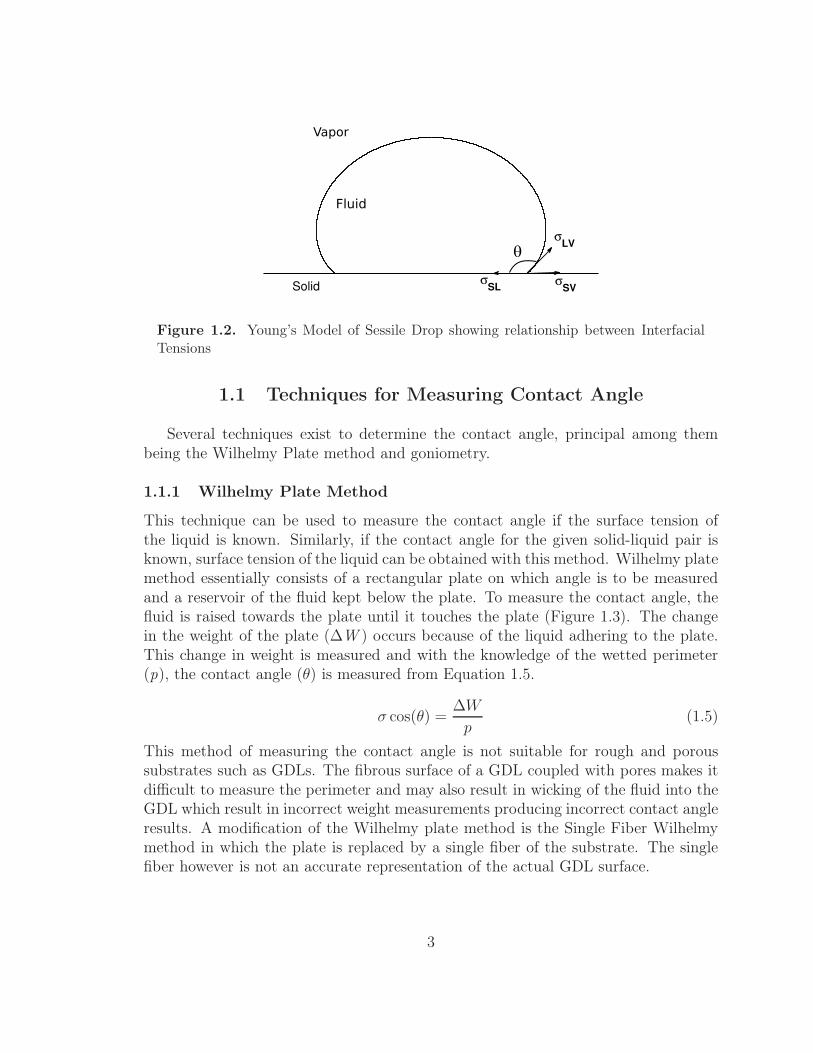
Figure 4.2 shows the stage of the experimental apparatus with the heat enclo-sure installed. The top of the stage consists of a copper block which is heated byfour thermo-electric heaters (Marlow Industries DT12-6-01L). The temperature iscontrolled by varying the voltage across the heaters. The heat enclosure consists oftwo glass windows through which drop images are taken. The glass is coated withIndium-Tin Oxide which is heated by passing current through it. Heating of the glassprevents condensation of water vapor at higher temperatures on the glass when theenclosure is humidified.

23

ITO coated

Glass

Microscope

Thermo-electric

coolers

Figure 4.2. Image of the stage with enclosure

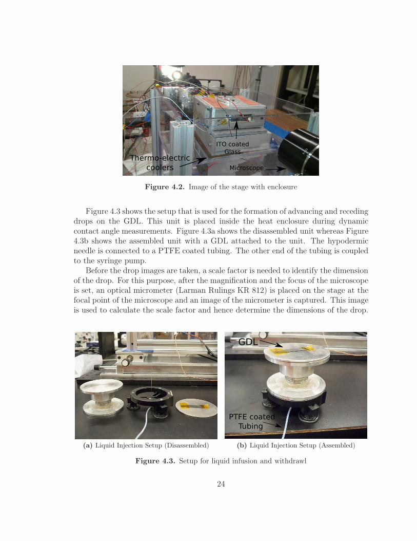
Figure 4.3 shows the setup that is used for the formation of advancing and recedingdrops on the GDL. This unit is placed inside the heat enclosure during dynamiccontact angle measurements. Figure 4.3a shows the disassembled unit whereas Figure4.3b shows the assembled unit with a GDL attached to the unit. The hypodermicneedle is connected to a PTFE coated tubing. The other end of the tubing is coupledto the syringe pump.

Before the drop images are taken, a scale factor is needed to identify the dimensionof the drop. For this purpose, after the magnification and the focus of the microscopeis set, an optical micrometer (Larman Rulings KR 812) is placed on the stage at thefocal point of the microscope and an image of the micrometer is captured. This imageis used to calculate the scale factor and hence determine the dimensions of the drop.

(a) Liquid Injection Setup (Disassembled)

GDL

PTFE coated

Tubing

(b) Liquid Injection Setup (Assembled)

Figure 4.3. Setup for liquid infusion and withdrawl

24

4.2 Static Measurement

To measure the static contact angle, a drop of liquid is formed on the tip of thehypodermic needle attached to a screw syringe. The syringe is fastened to a standwhich reduces any irregularities that are produced by manual drop deposition. Thesubstrate is then raised till it touches the drop using the Y control of the stage.The drop is the then brought into the field of view and onto the focal point of themicroscope by x-y translation of the stage and image is captured.

4.3 Dynamic Contact Angle Measurement

For measurement of advancing contact angle, syringe pump is used to inject fluidcontinuously at a constant rate. The GDL substrate is attached to the top of alu-minum plate using Kapton tape. A small hole is punched on the GDL. The size of thepiercing is kept close to the diameter of the needle used for injecting the liquid. Thisis done as safety precaution to prevent the fluid from seeping through the hole andbeneath the GDL. A series of images is captured at constant time rate from whichadvancing contact angles are obtained. At the end of the sequence, the syringe pumpis reversed and water is withdrawn from the drop.

4.4 Humidity Control

As the temperature increases the amount of water vapor in the air needed for satu-ration increases. If the air is not humidified, the water drops formed for measurementswill evaporate and hence the obtained contact angle will deviate from the actual one.Humidity is increased by placing water filled containers in the heat enclosure. Tocheck and the rate of evaporation, a very small droplet of water (approximately 2-3µl) is injected in the chamber at set temperature and the time required for the dropto evaporate is measured. Evaporation rate of less than 0.5µl/min, was consideredsatisfactory for the experiment to be carried on.

Sessile drops are formed by injecting water through a small hole in the GDLsubstrate by a hypodermic needle. Teflon tubing is used to pass water from thesyringe to the needle. The temperature of the enclosure is increased by increasingthe voltage across the thermo-electric heaters. Once the plate, on which the GDLsubstrate is kept, reaches the desired temperature, the voltage is kept constant andthe enclosure is kept in the same state for a period of 20-30 min. This allows theentire chamber to attain an equilibrium temperature. Around 5-6 inches of the tube ispresent in the heat chamber and is in contact with the heated copper plate allowingthe water to attain the equilibrium temperature. This ensures the temperature ofwater is same as that of experimental temperature.

25

Chapter 5. Results

With aim to understand the wetting characteristics of fuel cells, different GDL sampleswere tested under static and dynamic conditions and also at different temperatures.The GDL samples with composition are shown in Table 5.1. SEM images of the testedsamples in shown in Figure 5.1. PTFE coating in the samples is seen as the webbingin between the fibers. Apart from Freudenberg which has intertwined structure, allother samples consists of carbon fibers. Pore size distribution for three samples isshown in Table 5.2.

Table 5.1. GDL samples tested

Baseline Mitsubishi MRC 105 9% PTFE (weight) with MPLSGL SGL 25 BCFreudenberg Freudenberg H2315 with MPLToray Toray TFP-H-060 7% PTFE

Table 5.2. Pore size distribution of the tested GDL samples (Nishith Parikh, MTU,unpublished data)

SGL Freudenberg TorayAverage Pore Radius (µm) 8.25 15.92 13.2

Standard Deviation 8 19.5 9.75

26

(a) Mitsubishi (b) SGL

(c) Freudenberg (d) Toray

Figure 5.1. SEM images of GDL samples tested for contact angle measurement

5.1 Asymmetry in Drop Profile

The surface of a GDL is highly rough and porous. The contact angle obtainedon such a surface becomes dependent on the profile of the surface where the drop isdeposited. This results in different contact angles on the left and right side of thedrop. Figure 5.2 shows the image of a water drop on Toray obtained during advancingcontact angle measurements. From the figure, it is seen that the contact angle at theleft side of the drop is lower than the angle on the right side of the drop. Duringdynamic contact angle measurements, in many runs, pinning of the drop on one sideoccured while the movement of the contact line would take place on the other side.For such cases, only the data on the side with contact line movement is considered.

27

Table 5.3. Difference in Contact Angle for Left and Right Side of Drop.Fluid: Water, Substrate: Toray

Temperature Equatorial θ θ Difference(°C) Radius (cm) Left Right in θ

25

0.109 153.8 152.7 1.10.088 153.7 151.9 1.80.11 156.2 153.1 3.10.100 154.0 155.8 1.80.124 151.8 154.0 3.2

55

0.080 153.9 152.5 1.60.127 158.0 153.5 4.50.089 152.1 151.7 0.40.088 154.5 153.9 0.60.923 154.8 155.5 0.7

85

0.086 154.2 152.8 1.10.103 153.7 156.4 0.70.093 154.6 155.8 1.20.096 153.1 153.7 0.60.089 153.3 151.7 1.6

Figure 5.2. Difference in θ between left and right side of drop

28

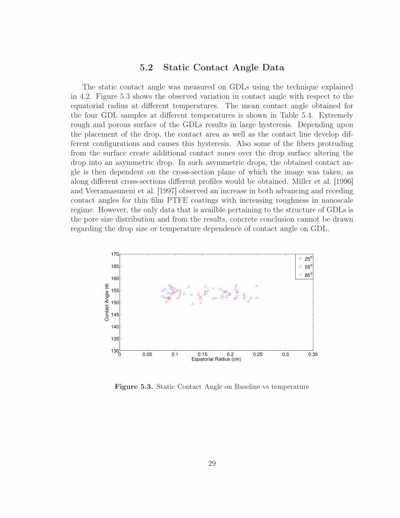
5.2 Static Contact Angle Data

The static contact angle was measured on GDLs using the technique explainedin 4.2. Figure 5.3 shows the observed variation in contact angle with respect to theequatorial radius at different temperatures. The mean contact angle obtained forthe four GDL samples at different temperatures is shown in Table 5.4. Extremelyrough and porous surface of the GDLs results in large hysteresis. Depending uponthe placement of the drop, the contact area as well as the contact line develop dif-ferent configurations and causes this hysteresis. Also some of the fibers protrudingfrom the surface create additional contact zones over the drop surface altering thedrop into an asymmetric drop. In such asymmetric drops, the obtained contact an-gle is then dependent on the cross-section plane of which the image was taken, asalong different cross-sections different profiles would be obtained. Miller et al. [1996]and Veeramasuneni et al. [1997] observed an increase in both advancing and recedingcontact angles for thin film PTFE coatings with increasing roughness in nanoscaleregime. However, the only data that is availble pertaining to the structure of GDLs isthe pore size distribution and from the results, concrete conclusion cannot be drawnregarding the drop size or temperature dependence of contact angle on GDL.

0 0.05 0.1 0.15 0.2 0.25 0.3 0.35130

135

140

145

150

155

160

165

170

Equatorial Radius (cm)

Conta

ct A

ngle

(θ)

25o

55o

85o

Figure 5.3. Static Contact Angle on Baseline vs temperature

29

Table 5.4. Mean static contact angle on GDLs at different temperatures

GDL 25° C 55° C 85° CMitsubishi 154.2 ±3 154.8 ±3.5 154.3 ±3.5SGL 25BC 151.7 ±4 149.1 ±4.5 150.5 ±3

Freudenberg 148.2 ±4.5 147.5 ±5 145.8 ±4.5Toray T060 154.7 ±3 153.6 ±2.5 154.3 ±2

5.3 Dynamic Contact Angle on GDL

Advancing and receding contact angles were measured on the samples and theresults are plotted in Figure 5.5 through 5.12. Figure 5.4 shows the variation incontact angle that was observed when multiple runs were carried out on the samesample. Different runs result in a wide range of advancing contact angles for thesame sample, the cause of which can be attributed to reasons explained previously inSection 5.2. On Baseline, Freudenberg and Toray, lower advancing contact angles wereobtained at higher temperatures. On SGL, a similar behavior is observed for smallerdrops. However at larger drop size, this change became negligible. Low contact anglesobserved on Baseline and Toray for small drop sizes is observed because of the contactline being pinned and the drops size being increased.

0.1 0.15 0.2 0.25 0.3 0.35130

135

140

145

150

155

160

165

170

Equatorial Radius (cm)

Conta

ct A

ngle

(θ)

Test 1

Test 2

Test 3

Figure 5.4. Advancing Contact Angle on Toray obtained for 3 test runs at 25° C

The receding contact angles however show a definite reduction in contact angleas the temperature is increased. As the drop volume is reduced, the contact linewould move towards the needle. But beyond a certain point, it would be pinned

30

0.1 0.15 0.2 0.25 0.3 0.35135

140

145

150

155

160

165

170

Equatorial Radius (cm)

Conta

ct A

ngle

(θ)

25o

55o

85o

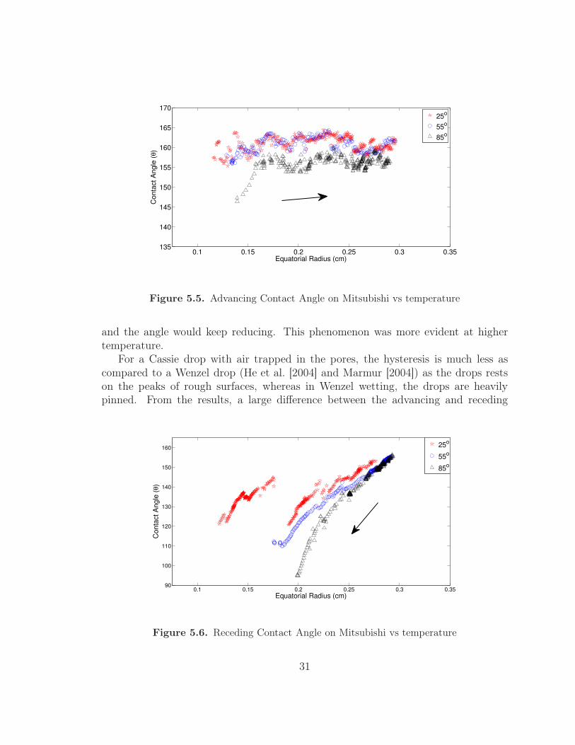
Figure 5.5. Advancing Contact Angle on Mitsubishi vs temperature

and the angle would keep reducing. This phenomenon was more evident at highertemperature.

For a Cassie drop with air trapped in the pores, the hysteresis is much less ascompared to a Wenzel drop (He et al. [2004] and Marmur [2004]) as the drops restson the peaks of rough surfaces, whereas in Wenzel wetting, the drops are heavilypinned. From the results, a large difference between the advancing and receding

0.1 0.15 0.2 0.25 0.3 0.3590

100

110

120

130

140

150

160

Equatorial Radius (cm)

Conta

ct A

ngle

(θ)

25o

55o

85o

Figure 5.6. Receding Contact Angle on Mitsubishi vs temperature

31

0.1 0.15 0.2 0.25 0.3 0.35135

140

145

150

155

160

165

170

Equatorial Radius (cm)

Conta

ct A

ngle

(θ)

25o

55o

85o

Figure 5.7. Advancing Contact Angle on SGL vs temperature

contact angles is observed and hence Wenzel wetting occurs on GDLs. This type ofwetting is also expected during the operation of fuel cell as water droplets are formedin the pores and on the GDL.

Another observation that was made during experiments was the vibration of sessiledrops on hydrophobic GDLs at larger drop volumes. For a sessile drop with highcontact angle, a large volume of the drop is supported on a small contact area. At

0.1 0.15 0.2 0.25 0.3 0.3590

100

110

120

130

140

150

160

Equatorial Radius (cm)

Conta

ct A

ngle

(θ)

25o

55o

85o

Figure 5.8. Receding Contact Angle on SGL vs temperature

32

0.1 0.15 0.2 0.25 0.3 0.35135

140

145

150

155

160

165

170

Equatorial Radius (cm)

Conta

ct A

ngle

(θ)

25o

55o

85o

Figure 5.9. Advancing Contact Angle on Freudenberg vs temperature

high drop volumes, typically 50-60 µl and above, the drop starts to vibrate becauseof the small vibrations that exists in the stage. This produces a large variation in themeasured contact angle at high drop volumes.

Receding contact angle at 25 °C on Mitsubishi GDL in Figure 5.6 is replotted inFigure 5.13c. A large discontinuity in contact angle is visible between the data pointsat A (Figure 5.13a) and B (Figure 5.13b). Smaller discontinuities are also visible

0.1 0.15 0.2 0.25 0.3 0.3590

100

110

120

130

140

150

160

Equatorial Radius (cm)

Conta

ct A

ngle

(θ)

25o

55o

85o

Figure 5.10. Receding Contact Angle on Freudenberg vs temperature

33

0.1 0.15 0.2 0.25 0.3 0.35135

140

145

150

155

160

165

170

Equatorial Radius (cm)

Conta

ct A

ngle

(θ)

25o

55o

85o

Figure 5.11. Advancing Contact Angle on Toray vs temperature

at points C, D and E. These jumps in contact angles occur when the contact linemoves rapidly from one position to another as the drop volume is reduced. Such avariation in contact angle due to rapid contact line motion is seen on other GDLsas well. Movement of the contact line also affect the advancing contact angle and itmanifests as the wavy or oscillatory trend in advancing contact angles. If the contactline is pinned or moves slowly, increase in the drop volume results in an increase in

0.1 0.15 0.2 0.25 0.3 0.3590

100

110

120

130

140

150

160

Equatorial Radius (cm)

Conta

ct A

ngle

(θ)

25o

55o

85o

Figure 5.12. Receding Contact Angle on Toray vs temperature

34

(a) A (b) B

0.1 0.15 0.2 0.25 0.3 0.3590

100

110

120

130

140

150

160

Equatorial Radius (cm)

Conta

ct A

ngle

(θ)

A

BC

D

E

25o

(c) Receding Contact Angle on Mitsubishi

Figure 5.13. Receding Contact Angle on Mitsubishi

the contact angle. Beyond a certain value, represented by the ‘peaks’, the contact linemoves rapidly which causes the contact angle to reduce. This phenomenon repeatsresulting in the oscillatory nature of the advancing contact angles.

35

Chapter 6. Conclusion

6.1 Summary

A program to determine the contact angle has been developed in MATLAB®.The program is automated to analyze multiple images which enables the calculationof advancing and receding contact angles. The contact angles are determined byfitting an ideal sessile drop profile curve obtained from the Laplace-Young equationwith the drop edge profile obtained from the drop images. The existing setup forthe measurement of contact angles was modified to incorporate a heat enclosure tomaintain the humidity at higher temperatures, which is necessary to prevent dropletevaporation. The new setup allows for injection and removal of water on the surfaceof GDL from which advancing and receding contact angles are obtained. Also, thesemeasurements were performed at different temperatures.

Accuracy in contact measurement is dependent on the drop deposition method,drop profile acquisition method and the accuracy in determining the solid-liquid in-terface. For drops with contact angles less than 90°on a smooth surface, solid-liquidinterface in determined with high accuracy making the results more accurate. ForGDLs, the high contact angles coupled with porous and rough fibrous surface restrictsthe accuracy in determining the contact angles.

Pixelation of drop images induces uncertainty in the contact angle measurement.As the drop edge obtained from image processing deviates more from the actual dropprofile, the uncertainty increases. Incorrect scale calculations produce no effect onthe contact angle obtained from images. At high contact angles, the inability in exactsolid-liquid interface detection further increases the error.

Advancing and receding and contact angles were collected for four GDL samplesat three different temperatures. Contact angle hysteresis that exists on GDL sam-ples hinders any concrete conclusion to be drawn from the experimental results foradvancing measurements. Advancing Contact angles obtained from multiple runs onGDLs result in a wide range of values which are comparable to that obtained at othertemperatures. A decrease in receding contact angle is observed as the temperatureis increased in all samples except SGL. Static contact angles obtained on GDL aredependent on the drop deposition technique.

36

6.2 Recommendations

Experiments to measure contact angles on GDLs should be performed with careand precision as the hysteresis produces a large variation in results. For a betterunderstanding of the wetting characteristics of the GDLs more experiments need tobe performed. This will allow a better statistical analysis of wetting in GDLs. Also,the experiments were performed on new or unused samples. Similar experimentsshould be conducted on ‘end-of-life’ samples as it may be helpful in understandingthe changes that take place in the wetting characteristics of GDLs during the lifecycle.

37

APPENDICES

38

Appendix A. Abbreviations

θ Contact angleθa Advancing contact angleθr Receding contact angleθC Cassie-Baxter’s contact angleθY Young’s contact angleθW Wenzel’s Contact Angleρ Densityσ Surface tensionσLV Liquid-vapor interfacial tensionσSL Solid-liquid interfacial tensionσSV Solid-vapor interfacial tension

ADSA Axisymmetric Drop Shape Analysisb Radius of curvature at apexB Non-dimensional radius of curvature at apexBo Bond numberc Capillary constantf Fractional Areag Gravitational constantGDL Gas Diffusion Layerp Perimeter∆P Change in pressure∆Pg Change in hydrostatic pressure∆Pσ Change in pressure across curved interfacePEM Proton Exchange MembranePTFE PolytetrafluoroethyleneR1 First principal radius of curvatureR2 Second principal radius of curvaturer Roughness factors Arc Length of drop surfaceS Non-dimensional arc Length of drop surface

39

∆W Change in weightx Horizontal distanceX Non-dimensional horizontal distancez Vertical distanceZ Non-dimensional vertical distance

40

Appendix B. Contact Angle

Measurement Programs

2.1 scale

% This function creates sc.mat which contains the scale factor for

the

% drop images. Enter the number of scales taken and import them.

% First zoom the images and select a suitable point on the leftmost

line

5 % which has uniformly varying pixel intensity. Then select the top or

the

% bottom part of the same line used initially. Do the same for

rightmost

% line. Enter the scale im mm for each image

%%

10

a = input('enter number of scales'); % Enter the number of scale

images.

scale_img = zeros(1,a);

pix_ind_x = −7:1:7; % Pixels used for spline fit in

x

15 nop = 30;

for j = 1:a

pix_x = zeros(nop,length(pix_ind_x));

pix_z = pix_x;

20

% Opens filepath of previously opened folder

oldpath=char(textread('filepath.dat','%s','whitespace',''));

% Lets user select full filepath of image graphically

25 [filename,filepath]=uigetfile([oldpath,'*.tif'],'open file:');

fid=fopen('filepath.dat','w');

fprintf(fid,'%s',filepath);

fclose(fid);

30 % Saves image to 'scale_fig' from specific filepath as selected

above

scale_fig = imread([filepath,filename]);

figure, imshow(scale_fig, [])

35 x_top = zeros(1,2); % x coordinate of top/bottom

z_top = zeros(1,2); % z coordinate of top/bottom

for k = 1:2

figure, imshow(scale_fig, [])

40 pause(7);

if k == 1

[xl, zl]=ginput(1); % Select scale points

else

[xr, zr]=ginput(1); % Select scale points

45 end

pause(5)

[x_top(k) z_top(k)] = ginput(1); % Select top point for

tilt

end

50 x_l(1:nop) = (xl−(nop/2)+1):1:(xl+nop/2);

z_l(1:nop) = zl;

x_r(1:nop) = (xr−(nop/2)+1):1:(xr+nop/2);

z_r(1:nop) = zr;

55 pixel_index_l = zeros(nop,length(pix_ind_x)); % Pixel intensity

saved here

pixel_index_r = zeros(nop,length(pix_ind_x)); % Pixel intensity

saved here

for k = 1:nop

pix_x_l(k,1:length(pix_ind_x)) = round(x_l(k)) + pix_ind_x;

60 pix_z_l(k,1:length(pix_ind_x)) = round(z_l(k));

for m = 1:(length(pix_ind_x))

pixel_index_l(k,m) = double(scale_fig(pix_z_l(k,m),

pix_x_l(k,m)));

end

65 end

for k = 1:nop

pix_x_r(k,1:length(pix_ind_x)) = round(x_r(k)) + pix_ind_x;

pix_z_r(k,1:length(pix_ind_x)) = round(z_r(k));

42

70

for m = 1:(length(pix_ind_x))

pixel_index_r(k,m) = double(scale_fig(pix_z_r(k,m),

pix_x_r(k,m)));

end

end

75

tilt = atand((z_top(2)−z_top(1))/(x_top(2)−x_top(1)));

multiplier = (z_top(2)−z_top(1))/cosd(tilt)−(z_top(2)−z_top(1));

n_pts = length(pix_ind_x);

80 x_opt_l = zeros(1,nop);

x_opt_r = zeros(1,nop);

% Fits a spline curve and finds location of minimum pixel

intensity

for k = 1:nop

85 base_pts_x = linspace(pix_x_l(k,1),pix_x_l(k,end),(n_pts*100)

+1);

spline_fit_x = spline(pix_x_l(k,:),pixel_index_l(k,:),

base_pts_x);

x_opt_l(k) = base_pts_x(find((spline_fit_x) == min(

spline_fit_x),1,'first'));

end

90 for k = 1:nop

base_pts_x = linspace(pix_x_r(k,1),pix_x_r(k,end),(n_pts*100)

+1);

spline_fit_x = spline(pix_x_r(k,:),pixel_index_r(k,:),

base_pts_x);

x_opt_r(k) = base_pts_x(find((spline_fit_x) == min(

spline_fit_x),1,'first'));

end

95

for k = 1:nop

pixels(k) = x_opt_r(k)−x_opt_l(k);

end

mm = input('Enter size of scale in mm: ');

100 cm = mm/10;

scale_all = zeros(nop,1);

for k = 1:nop

105 scale_all(k)=(abs(pixels(k)/cm))+((abs(z_top(2)−z_top(1)))/(abs(

x_l(k)−x_r(k))))*multiplier;

end

scale_img(1,j) = mean(scale_all);

end

43

110 save sc.mat scale_img;

% eof

44

2.2 needle_Scale

clc

clear

close all

no_p = 41; %Max permitted value 100

5 k = 1;

filepath = 'C:\ABCD\ABCD\'; % Enter filepath

filename = ('needle.tif'); % Enter filename

10 needle_img_uint = imread([filepath,filename]);

needle_img = double(needle_img_uint);

figure, imshow(needle_img, [])

15 pause(5)

[x, z]=ginput(4);

%% For left side

Z_l = (round(z(1)):1:round(z(2)));

20 Z_r = (round(z(3)):1:round(z(4)));

X_l = round((x(1)+x(2))/2);

X_r = round((x(3)+x(4))/2);

25 for j = 1:length(Z_l)

pixel_ind = X_l+ ((−no_p):1:(no_p));

for k = 1:(no_p*2+1)

30 pixel_data(k) = needle_img(Z_l(j),pixel_ind(k));

end

ind = find(pixel_data ≤ 80,1,'first');

35 mean_top = mean(pixel_data(1:ind));

mean_bot = mean(pixel_data((ind+1):end));

avg_int = (mean_top+mean_bot)/2;

40

base_pts = linspace(pixel_ind(1),pixel_ind(end),(no_p*200));

spline_fit = spline(pixel_ind,pixel_data,base_pts);

diff_int = abs(avg_int − spline_fit);

45

45

x_l(j) = base_pts(find(min(diff_int)==diff_int));

k = k+1;

end

50

%% For right side

for j = 1:length(Z_r)

55 pixel_ind = X_r+ ((−no_p):1:(no_p));

for k = 1:(no_p*2+1)

pixel_data(k) = needle_img(Z_r(j),pixel_ind(k));

end

60

ind = find(pixel_data ≤ 80,1,'first');

mean_top = mean(pixel_data(1:ind));

65

mean_bot = mean(pixel_data((ind+1):end));

avg_int = (mean_top+mean_bot)/2;

70 base_pts = linspace(pixel_ind(1),pixel_ind(end),(no_p*200));

spline_fit = spline(pixel_ind,pixel_data,base_pts);

diff_int = abs(avg_int − spline_fit);

75 x_r(j) = base_pts(find(min(diff_int)==diff_int));

k = k+1;

end

80 x_mean_l = mean(x_l);

x_mean_r = mean(x_r);

scale_pic = x_mean_r − x_mean_l;

85 load sc.mat

Diamater_needle = scale_pic/scale_img

% eof

46

2.3 Contact Angle Measurement Program

% Main program for contact angle measurement

clear

close

5 clc

%% Load scale

load sc.mat % loads previously saved scale

S_span=(0:.0001:3.5); % S_span is the step variable for ode45 solver

10

%% Analysis parameters

% These parameters affect the number of points and their location on

drop profile where calculations are done

No_ind = 21; % No of points where fit is calculated;

15 No_pt_slp = 16; % No of pts used for quadratic fit on each side

dif_slp = 3; % Difference in pixels for slope calcutation

cut_off = 17; % difference between the end pt on the drop and

last pt where error is calculated

%% Load properties and images

20

total_imgs = input('Enter total number of images'); % Number of

images

total_scl = input('Enter total number of scales'); % Number of

scales

expt_type = input('Entrer the type of experiment: 1−Static, 2−

Advancing'); % Type of Experiment

25 prefix_img = input('Enter a prefix if it exists (Press Enter if

nothing exist)'); % Prefix to image number

start_no_img = input('Enter Image Start Number'); % Number of 1st

image

range_lim = input('Range of images: For 1−10 Enter 1 For 11−99 Enter

2 For 101−999 Enter 3 '); % The Range of images

file_location = input('Enter Filepath (ex: C:\Folder\Folder\

Image_Folder\) :','s')'; % Location of images

file_location = file_location';

30

d_side = input('Enter side for More accuracy: Left = 1, Right = 2,

Both = 3 : '); % The side where more accuracy is needed

A = struct('scale_i',{},'folder_i',{},'file_i',{},'x_data_all_i',{},'

z_data_all_i',{},'x_l_i',{},'z_l_i',{},'x_r_i',{},'z_r_i',{},'

apex_x_i',{},'apex_z_i',{},'xpl_i',{},'zpl_i',{},'xpr_i',{},'zpr_i

47

',{}); % Structure for variables

35 Data = zeros(total_imgs,13); % Variable to store data

Err_data = zeros(total_imgs,72); % Variable to store data

for i = 1:total_imgs

40 [I,A(i).folder_i,A(i).file_i] = image_input(i,expt_type,

prefix_img,start_no_img,range_lim,file_location); % Images

input here

[BW,A(i).IC_i] = image_analysis(I); % Image

converted to Black and White

[boundary] = edge_detector(BW); % Boundary of

drop

[mean_l,mean_r,A(i).xpl_i,A(i).xpr_i,A(i).zpl_i,A(i).zpr_i ] =

plane( A(i).IC_i,boundary ); % Detects the solid−liquid

interface

[A(i).x_data_all_i,A(i).z_data_all_i,A(i).x_l_i,A(i).z_l_i,A(i).

x_r_i,A(i).z_r_i,A(i).apex_x_i,A(i).apex_z_i] = profile_split(

boundary,mean_l,mean_r); % Data points obtained

45 close all

display(A(i).file_i);

if total_scl > 1

scl = input('Enter scale number');

A(i).scale_i = scale_img(scl);

50 else

A(i).scale_i = scale_img(1,1);

end

end

55 clear I_sobel I BW boundary

%% Main loop

for r = 1:total_imgs

60

folder = A(r).folder_i;

file = A(r).file_i;

scale = A(r).scale_i;

IC = A(r).IC_i;

65 x_data_all = A(r).x_data_all_i;

z_data_all = A(r).z_data_all_i;

x_l = A(r).x_l_i;

z_l = A(r).z_l_i;

x_r = A(r).x_r_i;

70 z_r = A(r).z_r_i;

apex_x = A(r).apex_x_i;

apex_z = A(r).apex_z_i;

xpl_i = A(r).xpl_i;

48

zpl_i = A(r).zpl_i;

75 xpr_i = A(r).xpr_i;

zpr_i = A(r).zpr_i;

%% Indices of the points for left profile

80

ind_l = floor(0:((length(x_l)−cut_off)/(No_ind−1)):(length(x_l)−

cut_off));

ind_r = floor(0:((length(x_r)−cut_off)/(No_ind−1)):(length(x_r)−

cut_off));

85 %% This finds the points where the average of slope is calculated

if ind_l(2)< (No_pt_slp+2) || ind_r(2)< (No_pt_slp+2)

No_pt_slp = min(abs((ind_l(2)−1)),abs((ind_r(2)−1)));

end

90

x_avg_slope_l = zeros(No_ind,(2*No_pt_slp+1));

z_avg_slope_l = x_avg_slope_l;

95 for k = 2:No_ind

ind_slope = (−No_pt_slp:1:+No_pt_slp)+ind_l(k);

x_avg_slope_l(k,:) = x_l(ind_slope);

z_avg_slope_l(k,:) = z_l(ind_slope);

end

100

x_avg_slope_r = zeros(No_ind,(2*No_pt_slp+1));

z_avg_slope_r = x_avg_slope_r;

for k = 2:No_ind

105 ind_slope = (−No_pt_slp:1:+No_pt_slp)+ind_r(k);

x_avg_slope_r(k,:) = x_r(ind_slope);

z_avg_slope_r(k,:) = z_r(ind_slope);

end

110 %% Finds the average slope

avg_slope_l = zeros(No_ind,1);

if (2*No_pt_slp+1)−(2*dif_slp) == 0

115 dif_slp = dif_slp −1;

elseif (2*No_pt_slp+1)−(2*dif_slp) == −1

dif_slp = dif_slp −2;

end

120 for k = 2:No_ind

49

slope_temp = zeros(1,((2*No_pt_slp+1)−(2*dif_slp)));

for j = (dif_slp+1):(2*No_pt_slp+1)−dif_slp

% slope carried bet 3 pts

slope_temp(k,j−dif_slp) = (z_avg_slope_l(k,j+dif_slp)−

z_avg_slope_l(k,j−dif_slp))/(x_avg_slope_l(k,j+dif_slp

)−x_avg_slope_l(k,j−dif_slp));

end

125 avg_slope_l(k,1) = mean(slope_temp(k,:));

end

avg_slope_r = zeros(No_ind,1);

130 for k = 2:No_ind

slope_temp = zeros(1,((2*No_pt_slp+1)−(2*dif_slp)));

for j = (dif_slp+1):(2*No_pt_slp+1)−dif_slp

% slope carried bet 3 pts

slope_temp(k,j−dif_slp) = (z_avg_slope_r(k,j+dif_slp)−

z_avg_slope_r(k,j−dif_slp))/(x_avg_slope_r(k,j+dif_slp

)−x_avg_slope_r(k,j−dif_slp));

end

135 avg_slope_r(k,1) = mean(slope_temp(k,:));

end

%% check_l/r is used to vary the pixel direction

140 check_l = zeros(No_ind,1);

for k = 1:No_ind

if avg_slope_l(k,1) ≥0 && avg_slope_l(k,1)≤ tan(22.5*pi/180)

145

check_l(k) = 1;

elseif avg_slope_l(k,1) > tan(22.5*pi/180) && avg_slope_l(k

,1)≤ tan(67.5*pi/180)

check_l(k) = 2;

150 elseif avg_slope_l(k,1) > tan(67.5*pi/180) || avg_slope_l(k

,1)≤ tan(112.5*pi/180)

check_l(k) = 3;

elseif avg_slope_l(k,1) > tan(112.5*pi/180) && avg_slope_l(k

,1)≤ tan(157.5*pi/180)

155 check_l(k) = 4;

elseif avg_slope_l(k,1) > tan(157.5*pi/180) && avg_slope_l(k

,1) < 0

check_l(k) = 5;

end

50

160

end

check_r = zeros(No_ind,1);

165 for k = 1:No_ind

if avg_slope_r(k,1) ≥0 && avg_slope_r(k,1)≤ tan(22.5*pi/180)

check_r(k) = 1;

170 elseif avg_slope_r(k,1) > tan(22.5*pi/180) && avg_slope_r(k

,1)≤ tan(67.5*pi/180)

check_r(k) = 2;

elseif avg_slope_r(k,1) > tan(67.5*pi/180) || avg_slope_r(k

,1)≤ tan(112.5*pi/180)

175 check_r(k) = 3;

elseif avg_slope_r(k,1) > tan(112.5*pi/180) && avg_slope_r(k

,1)≤ tan(157.5*pi/180)

check_r(k) = 4;

elseif avg_slope_r(k,1) > tan(157.5*pi/180) && avg_slope_r(k

,1) < 0

180

check_r(k) = 5;

end

end

185

%% Finds the Data points on drop profile

[ x_sub_l,z_sub_l ] = pixel_data(x_data_all,z_data_all,x_l,z_l,

apex_x,apex_z,No_ind,No_pt_slp,ind_l,check_l,IC);

[ x_sub_r,z_sub_r ] = pixel_data(x_data_all,z_data_all,x_r,z_r,

apex_x,apex_z,No_ind,No_pt_slp,ind_r,check_r,IC);

190

%%

x_abs_l = zeros(No_ind,1);

z_abs_l = x_abs_l;

195 x_plot_l = zeros(size(x_sub_l));

z_plot_l = x_plot_l;

x_plot_r = zeros(size(x_sub_r));

z_plot_r = x_plot_r;

200 for k = 1:No_ind

[ x_abs_l(k,1),z_abs_l(k,1),x_plot,z_plot ] = abs_data_pts(

x_sub_l(k,:),z_sub_l(k,:),k);

51

x_plot_l(k,:) = x_plot;

z_plot_l(k,:) = z_plot;

end

205

x_abs_r = zeros(No_ind,1);

z_abs_r = x_abs_r;

for k = 1:No_ind

210 [ x_abs_r(k,1),z_abs_r(k,1),x_plot,z_plot ] = abs_data_pts(

x_sub_r(k,:),z_sub_r(k,:),k);

x_plot_r(k,:) = x_plot;

z_plot_r(k,:) = z_plot;

end

215 %% Restructuring points

true_apex_x = x_abs_r(1);

true_apex_z = z_abs_r(1);

220 apex_diff_x = apex_x − true_apex_x;

apex_diff_z = apex_z − true_apex_z;

x_lhs = x_abs_l − true_apex_x;

z_lhs = z_abs_l − true_apex_z;

225

x_rhs = x_abs_r − true_apex_x;

z_rhs = z_abs_r − true_apex_z;

230 x_plot_l = x_plot_l − true_apex_x;

z_plot_l = z_plot_l − true_apex_z;

x_plot_r = x_plot_r − true_apex_x;

z_plot_r = z_plot_r − true_apex_z;

235 %%

xpl = xpl_i − true_apex_x;

zpl = zpl_i − true_apex_z;

xpr = xpr_i − true_apex_x;

zpr = zpr_i − true_apex_z;

240

%% clear

clear avg_slope_l avg_slopr_r check_l check_r cut_l cut_r dh_l

dh_r

clear height_l height_r ind_l ind_r ind_slopr slope_temp

245 clear x_abs_l x_abs_r x_avg_slope_l x_avg_slope_r x_sub_l x_sub_r

clear z_abs_l z_abs_r z_avg_slope_l z_avg_slope_r z_sub_l z_sub_r

%% Scaling done here

52

250 [x_left_cm,z_left_cm, x_right_cm,z_right_cm,xl_cm,xr_cm,zl_cm,

zr_cm ] = scale_data(x_lhs,z_lhs,x_rhs,z_rhs,xpl,xpr,zpl,zpr,

scale);

%%

p_l = polyfit(xl_cm,zl_cm,1);

255

p_r = polyfit(xr_cm,zr_cm,1);

p_l(1) = −p_l(1);

260 %% Find optimum 'b' 'c'

if d_side == 1

[b_l,c_l] = bc_optimization(−x_left_cm,z_left_cm,No_ind);

[b_r,c_r] = bc_optimization_la(x_right_cm,z_right_cm,No_ind);

265 elseif d_side == 2

[b_l,c_l] = bc_optimization_la(−x_left_cm,z_left_cm,No_ind);

[b_r,c_r] = bc_optimization(x_right_cm,z_right_cm,No_ind);

else

[b_l,c_l] = bc_optimization(−x_left_cm,z_left_cm,No_ind);

270 [b_r,c_r] = bc_optimization(x_right_cm,z_right_cm,No_ind);

end

275 %% finds theta

[x_ly_l,z_ly_l,theta_l,vol_l,Err_theta_l] = contact_angle(b_l,c_l

,p_l,S_span,scale);

[x_ly_r,z_ly_r,theta_r,vol_r,Err_theta_r] = contact_angle(b_r,c_r

,p_r,S_span,scale);

%% Finds drop volume and theta

280 drop_volume = (vol_l+vol_r)/2;

[ eq_radius,wet_radius,drop_height_l,drop_height_r] =

drop_properties( x_ly_l,z_ly_l,x_ly_r,z_ly_r);

tilt_left = atand(−p_l(1));

tilt_right = atand(p_r(1));

285 %%

xl_n = −x_ly_l*scale;

zl_n = z_ly_l*scale;

xr_n = x_ly_r*scale;

zr_n = z_ly_r*scale;

290

x_l_n = xl_n + true_apex_x;

z_l_n = zl_n + true_apex_z;

53

x_r_n = xr_n + true_apex_x;

z_r_n = zr_n + true_apex_z;

295

%%

p_l_i = polyfit(xpl_i,zpl_i,1);

p_r_i = polyfit(xpr_i,zpr_i,1);

300

x_new_l = linspace(1,(xpl_i(end)+80),500);

x_new_r = linspace((xpr_i(1)−80),xpr_i(end),500);

305 z_new_l = polyval(p_l_i,x_new_l);

z_new_r = polyval(p_r_i,x_new_r);

figure

310 imshow(IC);

hold on

plot(x_l_n,z_l_n,'g',x_r_n,z_r_n,'g');

plot(x_new_l,z_new_l,'c',x_new_r,z_new_r,'c')

315 imagenumber = file(1:end−4);

imagefolder = [folder,'Images\',imagenumber,'_drop','.fig'];

saveas(gcf,imagefolder)

clear gcf

close all

320

%% Plots LY profile

figure

for k = 1:No_ind

hold on

325 plot(x_plot_l(k,:)/scale,z_plot_l(k,:)/scale,'r');

plot(x_plot_r(k,:)/scale,z_plot_r(k,:)/scale,'r');

end

330 plot((−x_ly_l),z_ly_l,'b',x_ly_r,z_ly_r,'b')

set(gca,'YDir','reverse');

axis([−.5 .5 −.5 .5]);

axis square

335 % Saves the figure

imagenumber = file(1:end−4);

imagefolder = [folder,'Images\',imagenumber,'.fig'];

saveas(gcf,imagefolder)

clear gcf

340 close all

54

%% Solution stored in the m file

Data(r,:) = [ eq_radius wet_radius drop_height_l

drop_height_r c_l c_r b_l b_r drop_volume tilt_left

tilt_right theta_l theta_r];

Err_data(r,:) = cat(1,Err_theta_l,Err_theta_r);

345 No_pt_slp = 16; % No of pts used for quadratic fit on

each side

dif_slp = 3;

end

%% Saves the result

350 datafolder = [folder,'Data\','Data'];

errfolder = [folder,'Data\','Err_data'];

strutfolder = [folder,'Data\','Struct_A'];

save(datafolder,'Data')

save(errfolder,'Err_data')

355 save(strutfolder,'A')

55

2.4 Functions

Here is a list of all of the functions used in the contact angle measurementprogram in alphabetical order.

2.4.1 abs_data_pts

function [ x_abs,z_abs,xx,pp ] = abs_data_pts(x,z,iter)

% This function fits a quadratic curve between the points and

% finds optimum point.

5 fit = 2; % Fit types

n = length(x);

if iter == 1

10 xx = x(1):((x(end)−x(1))/(n*50)):x(end);

p = polyfit(x,z,fit);

pp = polyval(p,xx);

z_abs = min(pp);

15 x_abs = xx(find(pp == z_abs)); %#ok<FNDSB>

xx = x;

pp = polyval(p,xx);

else

20

dx = diff(x);

if any(dx≤0)

zz = z(1):((z(end)−z(1))/(n−1)):z(end);

25 p = polyfit(z,x,fit);

pp = polyval(p,zz);

x_abs = pp((n+1)/2);

z_abs = zz((n+1)/2);

30

xx = pp;

pp = zz;

else

xx = x(1):((x(end)−x(1))/(n−1)):x(end);

35 p = polyfit(x,z,fit);

pp = polyval(p,xx);

x_abs = xx((n+1)/2);

z_abs = pp((n+1)/2);

56

40 end

end

end

45

%eof

2.4.2 bc_optimization

function [b_opt,c_opt] = bc_optimization(x_n,z_n,N)

S_span=(0:.001:6); % S_span is the step variable for ode45 solver

step_i = 0.1;

5

%%

c = 13.45;

[b_initial] = Initial_guess(x_n,z_n,c,N);

Bini = b_initial*(c^.5) ;

10

if Bini ≤ .2005

step_i = (Bini−0.005)/2;

end

15 Bnew = [(Bini−2*step_i) (Bini−step_i) (Bini) (Bini+step_i) (Bini+2*step_i)];

C = zeros(1,5);

err = zeros(1,5);

for j = 1:length(Bnew);

20 [ C(j),err(j) ] = cfinder(Bnew(j),c,x_n,z_n,N,S_span );

end

ind = find(min(abs(err))==abs(err));

25 Cnew = zeros(1,5);

errnew = Cnew;

%%

30 while (step_i)>0.0001

if ind == 1

57

Bnew1 = [(Bini−6*step_i) (Bini−5*step_i) (Bini−4*step_i) (

Bini−3*step_i) (Bini−2*step_i)];

Cnew(5) = C(1);

35 errnew(5) = err(1);

condn = 1;

elseif ind == 5

Bnew1 = [(Bini+2*step_i) (Bini+3*step_i) (Bini+4*step_i) (

Bini+5*step_i) (Bini+6*step_i)];

40 condn = 2;

Cnew(1) = C(5);

errnew(1) = err(5);

else

45 Bnew1 = [(Bnew(ind)−step_i) (Bnew(ind)−.5*step_i) (Bnew(ind))

(Bnew(ind)+.5*step_i) (Bnew(ind)+step_i)];

condn = 3;

Cnew(1) = C(ind−1);

Cnew(3) = C(ind);

Cnew(5) = C(ind+1);

50 errnew(1) = err(ind−1);

errnew(3) = err(ind);

errnew(5) = err(ind+1);

end

55 %%

if condn == 1

for j = 1:4

[ Cnew(j),errnew(j) ] = cfinder(Bnew1(j),c,x_n,z_n,N,

S_span );

60 end

elseif condn ==2

for j = 2:5

[ Cnew(j),errnew(j) ] = cfinder(Bnew1(j),c,x_n,z_n,N,

S_span );

end

65 elseif condn == 3

for j = [2,4]

[ Cnew(j),errnew(j) ] = cfinder(Bnew1(j),c,x_n,z_n,N,

S_span );

end

end

70

ind = find(min(abs(errnew))==abs(errnew));

if length(ind)>1

ind = round(mean(ind));

75 end

58

C = Cnew;

err = errnew;

step_i = step_i/2;

80

Bini = Bnew1(3);

Bnew = Bnew1;

end

85

c_opt = Cnew(ind);

B_opt = Bnew1(ind);

b_opt = B_opt/(c_opt^.5);

90 end

% eof

2.4.3 bc_optimization_la

function [b_opt,c_opt] = bc_optimization_la(x_n,z_n,N)

% Optimization with low accuracy for faster processing

S_span=(0:.001:6); % S_span is the step variable for ode45 solver

5 step_i = 0.1;

%%

c = 13.45;

10 [b_initial] = Initial_guess(x_n,z_n,c,N);

Bini = b_initial*(c^.5) ;

if Bini ≤ .2005

15 step_i = (Bini−0.005)/2;

end

Bnew = [(Bini−2*step_i) (Bini−step_i) (Bini) (Bini+step_i) (Bini+2*step_i)];

20 C = zeros(1,5);

err = zeros(1,5);

for j = 1:length(Bnew);

59

[ C(j),err(j) ] = cfinder(Bnew(j),c,x_n,z_n,N,S_span );

25 end

ind = find(min(abs(err))==abs(err));

Cnew = zeros(1,5);

30 errnew = Cnew;

%%

while (step_i)>0.005

35

if ind == 1

Bnew1 = [(Bini−6*step_i) (Bini−5*step_i) (Bini−4*step_i) (

Bini−3*step_i) (Bini−2*step_i)];

Cnew(5) = C(1);

40 errnew(5) = err(1);

condn = 1;

elseif ind == 5

Bnew1 = [(Bini+2*step_i) (Bini+3*step_i) (Bini+4*step_i) (

Bini+5*step_i) (Bini+6*step_i)];

45 condn = 2;

Cnew(1) = C(5);

errnew(1) = err(5);

else

50 Bnew1 = [(Bnew(ind)−step_i) (Bnew(ind)−.5*step_i) (Bnew(ind))

(Bnew(ind)+.5*step_i) (Bnew(ind)+step_i)];

condn = 3;

Cnew(1) = C(ind−1);

Cnew(3) = C(ind);

Cnew(5) = C(ind+1);

55 errnew(1) = err(ind−1);

errnew(3) = err(ind);

errnew(5) = err(ind+1);

end

60

%%

if condn == 1

for j = 1:4

65 [ Cnew(j),errnew(j) ] = cfinder(Bnew1(j),c,x_n,z_n,N,

S_span );

end

elseif condn ==2

for j = 2:5

60

[ Cnew(j),errnew(j) ] = cfinder(Bnew1(j),c,x_n,z_n,N,

S_span );

70 end

elseif condn == 3

for j = [2,4]

[ Cnew(j),errnew(j) ] = cfinder(Bnew1(j),c,x_n,z_n,N,

S_span );

end

75 end

%% % % % % % % % % % %

ind = find(min(abs(errnew))==abs(errnew));

80

if length(ind)>1

ind = round(mean(ind));

end

85 C = Cnew;

err = errnew;

step_i = step_i/2;

Bini = Bnew1(3);

90 Bnew = Bnew1;

end

%%

95 c_opt = Cnew(ind);

B_opt = Bnew1(ind);

b_opt = B_opt/(c_opt^.5);

100 end

% eof

2.4.4 cfinder

function [ C,err ] = cfinder(Bini,c,x_n,z_n,N,S_span )

% This function finds the optimum `c' for given B

b = Bini/(c^.5);

5

61

[S,Y] = ode45(@laplace,S_span,[0 1e−100 0],[],b,c); % may need to

increase second input if curve does not loop

Z=Y(:,1);

10 i=1;

while Z(i)<Z(i+1); % finds where contact angle is 180 degrees (

cutoff point)

i=i+1;

end;

15 x_ly(1:i,1)=Y(1:i,2); % Drop height dimensionless

z_ly(1:i,1)=Y(1:i,1); % Drop x dimension dimensionless

clear S_ly S Z Y x_ly_or_c z_ly_or_c

20 %%

iter = 1;

c1 = 10;

c2 = 20;

25

x_lynew = x_ly/(c1^.5);

z_lynew = z_ly/(c1^.5);

[error_profile1] = error_drop_new_w_sign(x_n,z_n,x_lynew,z_lynew,N );

clear x_lynew z_lynew

30

x_lynew = x_ly/(c2^.5);

z_lynew = z_ly/(c2^.5);

[error_profile2] = error_drop_new_w_sign(x_n,z_n,x_lynew,z_lynew,N );

%#ok<NASGU>

clear x_lynew z_lynew

35

close all

while iter ≤16

c3 = (c1+c2)/2;

x_lynew = x_ly/(c3^.5);

40 z_lynew = z_ly/(c3^.5);

[error_profile] = error_drop_new_w_sign(x_n,z_n,x_lynew,z_lynew,N

);

clear x_lynew z_lynew

if error_profile*error_profile1<0

45 c2 = c3;

error_profile2 = error_profile; %#ok<NASGU>

else

c1 = c3;

error_profile1 = error_profile;

50 end

62

iter = iter+1;

end

C = c3;

err =abs( error_profile);

55 clear x_ly z_ly S Z Y

end

% eof

2.4.5 cfinder_la

function [ C,err ] = cfinder_la(Bini,c,x_n,z_n,N,S_span )

%UNTITLED2 Summary of this function goes here

% Detailed explanation goes here

5 b = Bini/(c^.5);

[S,Y] = ode45(@laplace,S_span,[0 1e−100 0],[],b,c); % may need to

increase second input if curve does not loop

10 Z=Y(:,1);

i=1;

while Z(i)<Z(i+1); % finds where contact angle is 180 degrees (cutoff

point)

i=i+1;

15 end;

x_ly(1:i,1)=Y(1:i,2);%/(c^.5); % Drop height dimensionless

z_ly(1:i,1)=Y(1:i,1);%/(c^.5); % Drop x dimension

dimensionless

20

clear S_ly S Z Y x_ly_or_c z_ly_or_c

25 %%

iter = 1;

c1 = 10;

c2 = 19;

63

30

x_lynew = x_ly/(c1^.5);

z_lynew = z_ly/(c1^.5);

[error_profile1] = error_drop_new_w_sign(x_n,z_n,x_lynew,z_lynew,N );

clear x_lynew z_lynew

35

x_lynew = x_ly/(c2^.5);

z_lynew = z_ly/(c2^.5);

[error_profile2] = error_drop_new_w_sign(x_n,z_n,x_lynew,z_lynew,N );

%#ok<NASGU>

40 clear x_lynew z_lynew

close all

while iter ≤9

45 c3 = (c1+c2)/2;

x_lynew = x_ly/(c3^.5);

z_lynew = z_ly/(c3^.5);

[error_profile] = error_drop_new_w_sign(x_n,z_n,x_lynew,z_lynew,N

);

clear x_lynew z_lynew

50 if error_profile*error_profile1<0

c2 = c3;

error_profile2 = error_profile; %#ok<NASGU>

else

c1 = c3;

55 error_profile1 = error_profile;

end

% atr(iter) = error_profile;

iter = iter+1;

60 end

C = c3;

err =abs( error_profile);

% close all

65 clear x_ly z_ly S Z Y

70

end

64

2.4.6 contact_angle

function [x_ly_profile,z_ly_profile,theta,drop_vol,Err_t] =

contact_angle(b,c,p,S_span,scale )

% This function finds the final contact angle

[S,Y] = ode45(@laplace,S_span,[0 1e−100 0],[],b,c); % may need to

increase second input if curve does not loop

5 Z = Y(:,1);

i = 1;

while Z(i)<Z(i+1); % finds where contact angle is 180 degrees (cutoff

point)

i = i+1;

10 end

x_ly = zeros(i,1);

z_ly = zeros(i,1);

15 x_ly(1:i,1)=Y(1:i,2)/(c^.5); % Drop height dimensionless

z_ly(1:i,1)=Y(1:i,1)/(c^.5); % Drop x dimension

dimensionless

j = 1;

20 while(z_ly(j) ≤ (p(1)*x_ly(j)+p(2)))&& j<(i−10) ;

j = j+1;

end

ind_end = j;

25 x_ly_profile = x_ly(1:ind_end);

z_ly_profile = z_ly(1:ind_end);

angle = Y(ind_end,3)*180/pi; % Angle

30 theta = angle;

drop_vol = volume(z_ly,x_ly,z_ly_profile(end));

drop_height = z_ly_profile(end);

35

%%

Err_t = zeros(1,51); % Error matrix for interface correction

for j = −25:1:25

Err_t(1,j) = Y(find(z_ly ≤ drop_height+j/scale,1,'last'));

40 end

65

end

% eof

2.4.7 drop_properties

function [ eq_rad,wet_rad,drop_ht_l,drop_ht_r] = drop_properties( x_l

,z_l,x_r,z_r)

% Finds physical drop properties

eq_rad = (max(abs(x_l)) + max(abs(x_r)))/2;

5 wet_rad = (abs(x_l(end) + abs(x_r(end))))/2;

drop_ht_l = z_l(end);

drop_ht_r = z_r(end);

10 end

% eof

2.4.8 edge_detector

function [flip_bound]=edge_detector(Black_White)

% This function converts the image into grayscale

% from Russell Stacy (2009)

5 boundary_full = bwtraceboundary(Black_White,[1,1],'S'); % Find total

boundary of image

bound1 = boundary_full(find(boundary_full(:,2)==(length(Black_White

(1,:))−1), 1, 'last' ):length(boundary_full(:,1))−max(

boundary_full(:,1)),1); % trim the full boundary of column one to

eliminate the image edge

bound2 = boundary_full(find(boundary_full(:,2)==(length(Black_White

(1,:))−1), 1, 'last' ):length(boundary_full(:,1))−max(

boundary_full(:,1)),2); % trim the full boundary of column two to

eliminate the image edge

10

66

bound = [bound2,bound1]; % Recombine the two colums to form a

vector of values [x,y]

flip_bound = flipud(bound); % The "bound" vector is in reverse order

of data points from right to left. flipud() flips the vectors to

follow data points from left to right

end

15

% eof

2.4.9 error

function [error_profile] = error_drop(x_cm,z_cm,x_ly,z_ly,N )

% Finds the error in the drop profile

nop = 200; %Number fo points for fit

5 N_ly = length(x_ly);

distance1 = zeros(N_ly,1);

distance2 = zeros(nop,1);

distance_min = zeros(N,1);

distance_min_sign = zeros(N,1);

10

%%

weigh = 1;% sqrt(1:1:N);

for j = 2:N

15

for k = 1:N_ly

distance1(k,1) = sqrt( (x_cm(j)−x_ly(k))^2 + (z_cm(j)−z_ly(k)

)^2 );

end

20 ind_z = find(min(distance1)==distance1);

if ind_z == N_ly;

ind_z = ind_z−2;

end

25

ind = (ind_z−2):1:(ind_z+2);

p = polyfit(x_ly(ind),z_ly(ind),2);

x_cut = linspace(x_ly(ind(1)),x_ly(ind(end)),nop);

30 z_cut = polyval(p,x_cut);

for k = 1:nop

67

distance2(k) = sqrt((x_cut(k)−x_cm(j))^2+(z_cut(k)−z_cm(j))

^2);

end

35

ind_min = find(min(distance2)==distance2);

if x_cm(j) < x_cut(ind_min)

sign_error = 1;

40 else

sign_error = −1;

end

distance_min(j,1) = min(distance2)*weigh;

45 distance_min_sign(j,1) = sign_error*min(distance2)*weigh;

end

error_profile = sum(distance_min)*(abs(sum(distance_min_sign))/sum(

distance_min_sign));

50 end

% eof

2.4.10 exact_data

function [ x,z ] = exact_data(x_fit,z_fit,check,pixel_index)

% Based on input value of check, this function gives exact profile

data;

n_pts = length(x_fit);

5

if check == 1 || check == 5

base_pts_z = linspace(z_fit(1),z_fit(end),(n_pts*100)+1);

spline_fit_z = spline(z_fit,pixel_index,base_pts_z);

10

median_up_z = median(pixel_index(1:5));

median_dn_z = median(pixel_index((end−5):end));

intensity_z = (median_up_z+median_dn_z)/2;

15 dif_z = abs(intensity_z−spline_fit_z);

x = mean(x_fit);

z = base_pts_z(find(dif_z == min(dif_z),1,'first'));

68

20 elseif check == 2 || check == 4

base_pts_x = linspace(x_fit(1),x_fit(end),(n_pts*100)+1);

base_pts_z = linspace(z_fit(1),z_fit(end),(n_pts*100)+1);

25 spline_fit_x = spline(x_fit,pixel_index,base_pts_x);

median_up_x = median(pixel_index(1:5));

median_dn_x = median(pixel_index((end−5):end));

30 intensity_x = (median_up_x+median_dn_x)/2;

dif_x = abs(intensity_x−spline_fit_x);

x = base_pts_x(find(dif_x == min(dif_x),1,'first'));

z = base_pts_z(find(dif_x == min(dif_x),1,'first'));

35

elseif check == 3

base_pts_x = linspace(x_fit(1),x_fit(end),(n_pts*100)+1);

spline_fit_x = spline(x_fit,pixel_index,base_pts_x);

40

median_up_x = median(pixel_index(1:5));

median_dn_x = median(pixel_index((end−5):end));

intensity_x = (median_up_x+median_dn_x)/2;

45 dif_x = abs(intensity_x−spline_fit_x);

x = base_pts_x(find(dif_x == min(dif_x),1,'first'));

z = mean(z_fit);

50 end

end

% eof

2.4.11 image_analysis

function [Black_White,Trimmed_image]=image_analysis(Cropped_Image)

% This funtion produces the black and white image

co=10; % co is cutoff for top and bottom and left and right of image

5

69

thresh=0.85;

BW1=im2bw(Cropped_Image,thresh); % thresh is the threshold of the

image for converting to black and white.

10 Trimmed_image=Cropped_Image(co:length(Cropped_Image(:,1))−co,co:

length(Cropped_Image(1,:))−co);

Black_White=BW1(co:length(BW1(:,1))−co,co:length(BW1(1,:))−co);

end

15 % eof

2.4.12 image_input

function [Drop_Image,filepath,filename]=image_input(im_no,ex_type,

prefix_img,start_no,range_lim,filepath)

% This function reads the images

image_no = start_no+im_no−1; % Image number

5 image_names = num2str(image_no); % Image number in string

if ex_type == 2 % Adds 0s if required

if range_lim == 3

if image_no <10

10 image_names = ['0','0',image_names];

elseif image_no ≥10 && image_no <100

image_names = ['0',image_names];

end

elseif range_lim == 2

15 if image_no <10

image_names = ['0',image_names];

end

end

end

20

filename = [prefix_img,image_names,'.tif']; % Image name

Drop_Image = imread([filepath,filename]); % Image read

end

25

% eof

70

2.4.13 initial_guess

function [b_initial] = Initial_guess(x_n,z_n,c,N)

% Initial guess. Extracted from Russell Stacy (2009)

S_span = 0:.002:5;

5 up = N−5;

%%

iter = 1;

b1=3;

10 b2=.01;

bb=[b1 b2]; % range of b values to use

for j=1:2;

15

b=bb(j); % set b as individual values of b

[S,Y] = ode45(@laplace,S_span,[0 1e−100 0],[],b,c);

Z=Y(:,1);

20

i=1;

while Z(i)<Z(i+1);

i=i+1;

end;

25 x_ly(1:i,j)=Y(1:i,2)/(c^.5);

z_ly(1:i,j)=Y(1:i,1)/(c^.5);

end;

30 %% Error

[d1,z1]=min(abs(z_n(N−up)−z_ly(:,1))); % find indice of laplace data

that closely matches raw data

error_b1=x_n(N−up)−x_ly(z1,1); % finds relative horizontal

error of end of trim data

35 [d2,z2]=min(abs(z_n(N−up)−z_ly(:,2))); % find indice of laplace data

that closely matches raw data

error_b2=x_n(N−up)−x_ly(z2,2); % finds relative horizontal

error of end of trim data

if error_b1*error_b2>0 && error_b1<0;

fprintf('choose smaller b2 value');

40 elseif error_b1*error_b2>0 && error_b1>0;

fprintf('choose larger b1 value');

71

return

end;

45 error_b=min(abs([error_b1 error_b2]));

%% Minimization

c_change=.1;

50 b=(b1+b2)/2;

b3=b;

while (iter≤20);

clear x_ly z_ly S_ly Phi_ly Z

55

[S,Y] = ode45(@laplace,S_span,[0 1e−100 0],[],b3,c); % may need

to increase span of S if curve does not loop

Z=Y(:,1); % the first column of Y is the Z data. Needs to be

defined to find cutoff point below.

i=1;

60 while Z(i)<Z(i+1); % finds where contact angle is 180 degrees (

cutoff point)

i=i+1;

end;

% Output Variables

65

x_ly_1(1:i)=Y(1:i,2)/(c^.5); % Drop height

dimensionless

z_ly_1(1:i)=Y(1:i,1)/(c^.5); % Drop width

dimensionless

[d3,z3]=min(abs(z_n(N−up)−z_ly_1)); % find indice of laplace data

that closely matches raw data

70 error_b3=x_n(N−up)−x_ly_1(z3); % finds relative horizontal

error of end of trim data

if error_b3*error_b1>0;

b1=b3;

error_b1=error_b3;

75 error_b=error_b1;

else

b2=b3;

error_b2=error_b3;

error_b=error_b2;

80 end;

b=b3;

b3=(b1+b2)/2;

iter = iter+1;

72

85 end;

b_initial = b3;

end

2.4.14 laplace

%Derek Fultz and Russ Stacy

%7−24−07

%

% LAPLACE defines the ordinary differential equations to be solved.

5 % z=drop height

% x=distance from axis to drop interface

% phi=contact angle

% 1/b=radius of curvature at apex

% s=arc length

10 %

% NON−DIMENSIONALIZE Z,X,S,B USING C^(1/2)

% B=b*c^(1/2)

% X=x*c^(1/2)

% Z=z*c^(1/2)

15 % S=s*c^(1/2)

%

% No need to define X,Z,S for equations

%

% KEY OF VARIABLE DEFINITIONS FOR SYSTEM

20 % Z=y(1); Z'=dy(1); Z' is with respect to S

% X=y(2); X'=dy(2); X' is with respect to S

% phi=y(3); phi'=dy(3); phi' is with respect to S

%

% Z'=sin(phi)

25 % X'=cos(phi)

% phi'=2/B+Z−(sin(phi)/X)

function [dy]=laplace(s,y,m,n)

dy = zeros(3,1); % a column vector

30

B=m*n^.5; % non−dimensionalized curvature at apex

dy(1)=sin(y(3));

dy(2)=cos(y(3));

35 dy(3)=(2/B)+y(1)−(sin(y(3))/y(2));

73

end

% eof

2.4.15 plane

function [mean_left,mean_right,x_plane_left,x_plane_right,

z_plane_left,z_plane_right ] = plane( I,boundary )

% This function finds the Solid−Liquid Interface

ini_z = boundary(:,2);

5

z_left_temp = ini_z(1:10); % 10 pixels from left edge of

image

z_right_temp = ini_z(end−10:end); % 10 pixels from left edge of

image

plane_left_ini = round(mean(z_left_temp)); % Mean of left plane

10 plane_right_ini = round(mean(z_right_temp)); % Mean of right plane

apex_z_ind = (find(boundary(:,2)== min(boundary(:,2)),1,'first'));

x_left = boundary(1:apex_z_ind,1);

15 z_left = boundary(1:apex_z_ind,2);

x_right = boundary((apex_z_ind+1):end,1);

z_right = boundary((apex_z_ind+1):end,2);

20 cutoff_x_l = x_left(find(z_left == (plane_left_ini − 20),1,'last'));

cutoff_x_r = x_right(find(z_right == (plane_right_ini − 20),1,'first'

));

z_left_int = I((plane_left_ini−18):(plane_left_ini+18),1:cutoff_x_l)

;

z_right_int = I((plane_right_ini−18):(plane_right_ini+18),cutoff_x_r:

end);

25

z_left_img = double(z_left_int);

z_right_img = double(z_right_int);

%%

30

for j = 1:length(z_left_img(1,:))

for i = 1:(length(z_left_img(:,1))−4)

74

dz_left(i,j) = (z_left_img(i,j)−8*z_left_img(i+1,j)+8*z_left_img(i+3,j)−z_left_img(i+4,j))/12;

end

35 end

for j = 1:length(z_right_img(1,:))

for i = 1:(length(z_right_img(:,1))−4)

dz_right(i,j) = (z_right_img(i,j)−8*z_right_img(i+1,j)+8*z_right_img(i+3,j)−z_right_img(i+4,j))/12;

40 end

end

%%

45 for j = 1:length(z_left_img(1,:))

plane_left(j) = round(mean(find(abs(dz_left(:,j)) == max(abs(

dz_left(:,j))) )));

end

for j = 1:length(z_right_img(1,:))

50 plane_right(j) = round(mean(find(abs(dz_right(:,j)) == max(abs(

dz_right(:,j))) )));

end

%%

55 z_plane_left = plane_left + plane_left_ini−17;

z_plane_right = plane_right + plane_right_ini−17;

%%

60 I1 = I;

for j = 1:length(z_left_img(1,:));

I1(round(z_plane_left(j)),j)=255;

end

65 for j = 1:length(z_right_img(1,:));

k = cutoff_x_r + j −1;

I1(round(z_plane_right(j)),k)=226;

end

70 mean_left = round(mean(z_plane_left));

mean_right = round(mean(z_plane_right));

%%

75 p_l = polyfit(1:length(z_plane_left),z_plane_left,1);

p_r = polyfit(cutoff_x_r:length(I(1,:)),z_plane_right,1);

75

%%

80 x_plane_left = 1:length(z_plane_left);

x_plane_right = cutoff_x_r:length(I(1,:));

end

85 % eof

2.4.16 pixel_data

function [ x_sub,z_sub ] = pixel_data(x_all,z_all,x_pts,z_pts,apex_x,

apex_z,N,N_op,ind,check_xy,crop_im )

% This function gives the sub−pixel data for N_op points

x_mat = zeros(N,(2*N_op+1)); % here 21 pts of x are

stored (−10:10) for N points

5 z_mat = x_mat;

x_sub = x_mat; % here exact 21 pts of

x are stored (−10:10) for N points

z_sub = z_mat;

10 %%

for j = 1:N

if j == 1

apex_indice = round((find(z_all == 0,1,'first')+find(z_all ==

0,1,'last'))/2);

15 ind_pts = (−N_op:1:N_op) + apex_indice;

x_mat(1,:) = x_all(ind_pts);

z_mat(1,:) = z_all(ind_pts);

else

ind_pts = (−N_op:1:N_op) + ind(j);

20 x_mat(j,:) = x_pts(ind_pts);

z_mat(j,:) = z_pts(ind_pts);

end

end

25 x_mat = x_mat+apex_x; % apex added to make

compatible with image

z_mat = z_mat+apex_z;

76

pix_ind = 15; % no of points taken in

image for spline fit

pixel_index = zeros(1,(pix_ind)); % stores pixel data

30

for j = 1:N

check = check_xy(j);

if check == 1

pix_ind_z = −7:1:7;

35 for k = 1:(2*N_op+1)

pix_x(1,1:(pix_ind)) = x_mat(j,k);

pix_z = z_mat(j,k) + pix_ind_z;

for m = 1:(pix_ind)

pixel_index(1,m) = double(crop_im(pix_z(m),pix_x(m)))

;

40 end

[x_sub(j,k),z_sub(j,k)] = exact_data(pix_x,pix_z,check,

pixel_index);

end

elseif check == 2

45

pix_ind_x = −7:1:7;

pix_ind_z = 7:−1:−7;

for k = 1:(2*N_op+1)

50

pix_x = x_mat(j,k)+ pix_ind_x;

pix_z = z_mat(j,k)+ pix_ind_z;

for m = 1:(pix_ind)

55 pixel_index(1,m) = double(crop_im(pix_z(m),pix_x(m)))

;

end

[x_sub(j,k),z_sub(j,k)] = exact_data(pix_x,pix_z,check,

pixel_index);

end

60

elseif check == 3

pix_ind_x = −7:1:7;

65 for k = 1:(2*N_op+1)

pix_x(1,1:length(pix_ind_x)) = x_mat(j,k) + pix_ind_x;

pix_z(1,1:length(pix_ind_x)) = z_mat(j,k);

70 for m = 1:(pix_ind)

77

pixel_index(1,m) = double(crop_im(pix_z(m),pix_x(m)))

;

end

[x_sub(j,k),z_sub(j,k)] = exact_data(pix_x,pix_z,check,

pixel_index);

75 end

elseif check == 4

pix_ind_x = −7:1:7;

80 pix_ind_z = −7:1:7;

for k = 1:(2*N_op+1)

pix_x(1,1:length(pix_ind_x)) = x_mat(j,k)+ pix_ind_x;

85 pix_z(1,1:length(pix_ind_z)) = z_mat(j,k)+ pix_ind_z;

for m = 1:(pix_ind)

pixel_index(1,m) = double(crop_im(pix_z(m),pix_x(m)))

;

end

90 [x_sub(j,k),z_sub(j,k)] = exact_data(pix_x,pix_z,check,

pixel_index);

end

elseif check == 5

95 pix_ind_z = −7:1:7;

for k = 1:(2*N_op+1)

pix_x(1,1:length(pix_ind_z)) = x_mat(j,k);

100 pix_z(1,1:length(pix_ind_z)) = z_mat(j,k) + pix_ind_z;

for m = 1:(pix_ind)

pixel_index(1,m) = double(crop_im(pix_z(m),pix_x(m)))

;

end

105

[x_sub(j,k),z_sub(j,k)] = exact_data(pix_x,pix_z,check,

pixel_index);

end

end

110

end

end

78

115 %eof

2.4.17 profile_split

function [x_data_all,z_data_all,x_l,z_l,x_r,z_r,apex_x,apex_z] =

profile_split( boundary,mean_l,mean_r)

%%

apex_z = min(boundary(:,2)); %

Gives z position of apex

apex_x = boundary(round(mean(find(boundary(:,2) == apex_z))),1); %

Gives x position of apex

5

x_data_all = boundary(:,1) − apex_x; % all x data

z_data_all = boundary(:,2) − apex_z; % all z data

apex_ind = round((find(z_data_all == 0,1,'first')+find(z_data_all ==

0,1,'last'))/2);

10

z_left = z_data_all(1:apex_ind);

z_right = z_data_all((apex_ind+1):end);

z_cut_l = find(z_left == ((mean_l−20)−apex_z),1,'last');

15 z_cut_r = find(z_right == ((mean_r−20)−apex_z),1,'first')+apex_ind;

x_data = x_data_all(z_cut_l:z_cut_r);

z_data = z_data_all(z_cut_l:z_cut_r);

20 apex_ind_n = round((find(z_data == 0,1,'first')+find(z_data == 0,1,'

last'))/2);

x_l = x_data(apex_ind_n:−1:1); % Note apex is the start and the

end point

z_l = z_data(apex_ind_n:−1:1);

25 x_r = x_data(apex_ind_n:end);

z_r = z_data(apex_ind_n:end);

end

2.4.18 scale_data

79

function [x_left_cm,z_left_cm, x_right_cm,z_right_cm,xl_cm,xr_cm,

zl_cm,zr_cm ] = scale_data(x_left,z_left,x_right,z_right,xpl,xpr,

zpl,zpr,scale)

% Scale the data

x_left_cm = x_left/scale;

5 z_left_cm = z_left/scale;

x_right_cm = x_right/scale;

z_right_cm = z_right/scale;

10 xl_cm = xpl/scale;

xr_cm = xpr/scale;

zl_cm = zpl/scale;

zr_cm = zpr/scale;

15 end

% eof

2.4.19 volume

function [drop_vol] = volume(z_ly_1,x_ly_1,drop_height_nd)

% This function finds the volume using washers scheme

Z_ly_ind = find(z_ly_1 ≤ drop_height_nd); % Index of end point on

drop

5

Z_ly = z_ly_1(1:length(Z_ly_ind)); % End Z

X_ly = x_ly_1(1:length(Z_ly_ind)); % End X

V = zeros(length(Z_ly)−1,1); % Size of Volume matrix

10

for n = 2:length(Z_ly)

V(n−1) = pi*(((X_ly(n)+X_ly(n−1))/2)^2)*(Z_ly(n)−Z_ly(n−1));

end

15 drop_vol = sum(V)*1000;

end

% eof

80

2.5 images_reader

%% This program load the 'xxx_drop.fig' files to check for error

clear

clc

5

mult = 1;

image_no = 1; % Start image no

end_no = 100; % End image no

10 k = 0;

j = 1;

step_size = 1;

15 filepath = 'C:\ABCD\ABCD\Images\';

Image = image_no;

while image_no ≤ end_no

20

image_names = num2str(image_no);

if image_no <10

image_names = ['0','0',image_names];

25 elseif image_no ≥10 && image_no <100

image_names = ['0',image_names];

end

filename = ['A',image_names,'_drop','.fig'];

30

open([filepath,filename]);

l = input('');

if isempty(l)

35 Correction(j,1) = 0;

else

Correction(j,1) = l;

end

40 r = input('');

if isempty(r)

Correction(j,2) = 0;

else

Correction(j,2) = r;

81

45 end

close gcf

if step_size == 1

j = j+1;

50 image_no = image_no+mult*step_size;

elseif step_size == 2

Correction(j+1,:) = Correction(j,:);

j = j+2;

image_no = image_no+mult*step_size;

55 elseif step_size == 3

Correction(j+1,:) = Correction(j,:);

Correction(j+2,:) = Correction(j,:);

j = j+3;

image_no = image_no+mult*step_size;

60 elseif step_size == 4

Correction(j+1,:) = Correction(j,:);

Correction(j+2,:) = Correction(j,:);

Correction(j+3,:) = Correction(j,:);

j = j+4;

65 image_no = image_no+mult*step_size;

end

Image(j) = image_no;

end

70

save('C:\ABCD\ABCD\Data\Correction.mat','Correction')

% eof

82

2.6 Data_modifier

% Loads and does all the modifications

clc

clear

5 filepath = 'C:\ABCD\ABCD\';

mid1 = 26;

mid2 = 77;

10 %%

Data_file = [filepath,'Data\','Data.mat'];

Corr_file = [filepath,'Data\','Correction.mat'];

Err_file = [filepath,'Data\','Err_data.mat'];

15 D1 = load(Data_file);

C1 = load(Corr_file);

E1 = load(Err_file);

Vol = D1.Data(:,9,1);

20 Error_Data = E1.Err_data(:,:,1);

%%

Theta_l = D1.Data(:,12,1);

25 Theta_r = D1.Data(:,13,1);

plot(Vol,Theta_l,'ro',Vol,Theta_r,'bo')

legend('Left','Right')

30 Corr_l_1 = C1.Correction(:,1,1);

Corr_r_1 = C1.Correction(:,2,1);

%%

35 if length(Theta_l) 6= length(Corr_l_1)

fprintf('Dimensions of Corr1 mismatch')

Corr_l_1 = C1.Correction(1:length(Theta_l),1,1);

Corr_r_1 = C1.Correction(1:length(Theta_r),2,1);

end

40

%%

Correction_l = Corr_l_1;

Correction_r = Corr_r_1;

83

45

%%

for j = 1:length(Vol)

if Correction_r(j) == 0

50 Theta_r_mod(j,1) = Theta_r(j);

elseif round(Correction_r(j)) 6= Correction_r(j)

adder = (Correction_r(j)−floor(Correction_r(j)))*(Error_Data(

j,(mid2+ceil(Correction_r(j))))−Error_Data(j,(mid2+floor(

Correction_r(j)))));

Theta_r_mod(j,1) = Error_Data(j,(mid2+floor(Correction_r(j)))

)+adder;

55

else

Theta_r_mod(j,1) = Error_Data(j,(mid2+Correction_r(j)));

end

60

if Correction_l(j) == 0

Theta_l_mod(j,1) = Theta_l(j);

65 elseif round(Correction_l(j)) 6= Correction_l(j)

adder = (Correction_l(j)−floor(Correction_l(j)))*(Error_Data(

j,(mid1+ceil(Correction_l(j))))−Error_Data(j,(mid1+floor(

Correction_l(j)))));

Theta_l_mod(j,1) = Error_Data(j,(mid1+floor(Correction_l(j)))

)+adder;

70 else

Theta_l_mod(j,1) = Error_Data(j,(mid1+Correction_l(j)));

end

end

75

Final_Data = cat(2,Vol,Theta_l,Theta_r,Theta_l_mod,Theta_r_mod);

save([filepath,'Final_data.mat'],'Final_Data')

80

%%

figure

plot(Vol,Theta_l_mod,'ro',Vol,Theta_r_mod,'bo')

85 % eof

84

REFERENCES

James Larminie and Andrew Dicks. Fuel Cells Systems Explained. John Wiley &Sons Ltd„ 2003.

Jeffrey S. Allen. An analytical solution for determination of small contact angles fromsessile drops of arbitrary size. Journal of Colloid and Interface Science, 261(2):481– 489, 2003. ISSN 0021-9797.

A.F. Stalder, G. Kulik, D. Sage, L. Barbieri, and P. Hoffmann. A snake-based ap-proach to accurate determination of both contact points and contact angles. Col-

loids and Surfaces A: Physicochemical and Engineering Aspects, 286(1-3):92 – 103,2006. ISSN 0927-7757.

F. Bashforth and J.C. Adams. An Attempt to Test the Theories of Capillary Action by

Comparing the theoretical and Measured Forms of Drops of Fluid-Liquid. CambrideUniversity Press, London, 1883.

Stanley Hartland and Richard W. Hartley. Axisymmetric Fluid-Liquid Interfaces.Elsevier, 1976.

P. Cheng, D. Li, L. Boruvka, Y. Rotenberg, and A.W. Neumann. Automation of ax-isymmetric drop shape analysis for measurements of interfacial tensions and contactangles. Colloids and Surfaces, 43(2):151 – 167, 1990. ISSN 0166-6622. SelectedPapers from a Symposium on Recent Progress in Interfacial Tensiometry, held atthe Third Chemical Congress of North America.

Robert N. Wenzel. Resistance of solid surfaces to wetting by water. Industrial &

Engineering Chemistry, 28(8):988–994, August 1936. ISSN 0019-7866.

A. B. D. Cassie and S. Baxter. Wettability of porous surfaces. Trans. Faraday Soc.,40:546–551, 1944. ISSN 0014-7672.

Jaroslaw Drelich and Jan D. Miller. Modification of the cassie equation. Langmuir,9(2):619–621, February 1993. ISSN 0743-7463.

85

Russell Stacey. Contact angle measurement technique for rough surfaces. Master’sthesis, Michigan Technological University, 2009.

A. W. Neumann and Jan K. Spelt, editors. Applied Science Thermodynamics. MarcelDekker, Inc., 1996.

J. D. Miller, S. Veeramasuneni, J. Drelich, M. R. Yalamanchili, and G. Yamauchi.Effect of roughness as determined by atomic force microscopy on the wetting prop-erties of ptfe thin films. Polym Eng Sci, 36(14):1849–1855, 1996. ISSN 1548-2634.

S. Veeramasuneni, J. Drelich, J. D. Miller, and G. Yamauchi. Hydrophobicity of ion-plated ptfe coatings. Progress in Organic Coatings, 31(3):265 – 270, 1997. ISSN0300-9440.

Bo He, Junghoon Lee, and Neelesh A. Patankar. Contact angle hysteresis on roughhydrophobic surfaces. Colloids and Surfaces A: Physicochemical and Engineering

Aspects, 248(1-3):101 – 104, 2004. ISSN 0927-7757.

Abraham Marmur. The lotus effect: Superhydrophobicity and metastability. Lang-

muir, 20(9):3517–3519, April 2004. ISSN 0743-7463.

86