Embed Size (px)
Citation preview
Static and dynamic behaviour of mechanical controlsystems of slow-running wind turbinesBos, Kees; Schoonhoven, Huib; Verhaar, J.
Published: 01/01/1983
Document VersionPublisher’s PDF, also known as Version of Record (includes final page, issue and volume numbers)
Please check the document version of this publication:
• A submitted manuscript is the author's version of the article upon submission and before peer-review. There can be important differencesbetween the submitted version and the official published version of record. People interested in the research are advised to contact theauthor for the final version of the publication, or visit the DOI to the publisher's website.• The final author version and the galley proof are versions of the publication after peer review.• The final published version features the final layout of the paper including the volume, issue and page numbers.
Link to publication
Citation for published version (APA):Bos, K., Schoonhoven, H., & Verhaar, J. (1983). Static and dynamic behaviour of mechanical control systems ofslow-running wind turbines. (TU Eindhoven. Vakgr. Transportfysica : rapport; Vol. R-592-D). Eindhoven:Technische Hogeschool Eindhoven.
General rightsCopyright and moral rights for the publications made accessible in the public portal are retained by the authors and/or other copyright ownersand it is a condition of accessing publications that users recognise and abide by the legal requirements associated with these rights.
• Users may download and print one copy of any publication from the public portal for the purpose of private study or research. • You may not further distribute the material or use it for any profit-making activity or commercial gain • You may freely distribute the URL identifying the publication in the public portal ?
Take down policyIf you believe that this document breaches copyright please contact us providing details, and we will remove access to the work immediatelyand investigate your claim.
Download date: 03. Jun. 2018
Static and dynamic behaviour of
mechanical control systems of
slow-running wind turbines.
April 1983
R 592 D
Kees Bos
Huib Schoonhoven
Jan Verhaar
DOCUMENT ATIECENTRUM B.O.S, - THE.
class.
dv.
datum
Under responsibility of
Prof. Dr. C.A. ten Seldam.
University of Amsterdam.
Pr>eface.
This ~epo~t is the ~esult of p~actical work as a part of a study in
expe~imental physics at the Unive~sity of Amste~dam (UvA) by th~ee
students.
The majo~ part of this ~epo~t conce~s the dynamic behavio~ of-wind
t~bines equiped with a mechanical cont~ol system in particular the
so-called inclined hinged vane system.
The outline of this s~ey was established in consultation with the
Stee~ing committee Windene~gy Developing countries (SWD). This orga
nisation is a.o. concerned with the possibiZities of wind energy uti
lisation in developing countries. Cooperative members of this o~ga
nisation are a.o. the Eindhoven University of Technology (THE) and
DHV~ consulting engineers at Ame~sfoo~t.
As for the UvA this project was car~ied out unde~ responsibility of
Dr. C.A. ten SeZdam~ Professo~ of Physics at the Van de~ Waals institute.
The authors wish to express their gratitude to Ir. A. Adema (DHV)~
Ir. P.T. Smulders and I~. H. van der Spek (THE) for thei~ construc
tive advice, and, of co~se, to Dr. Ten Seldam for his close guidance
and neve~lasting patience. F~thermore they wish to thank the mechani
cal wo~kshop fo~ their technical assistance and Mrs. J. Thomas for
he~ st~aight-fo~ard manner of se~ving tea and coffee.
Summa~y.
A mathematiaal model of a wind turbine with a meahaniaal aont~ol
system has been set up in o~de~ to inve8tigate its dynamia beha
vio~.
A aompute~ p~og~am to enabLe simuLation of this behavio~ has
been developed.
WindtunneL expe~iment8, using a saale model, have been pe~formed
on both ~oto~ and vanes to determine the nat~e of ae~odynamia
fo~aes and to~ques aating on them. Using the same equipment
~egi8t~ations have been obtained of the 8tatia and dynamia be
haviou~.
Comp~iBon of ~esults of the aompute~ modeL and expe~iments showed
aaaeptabZe ag~eement.
Contents.
Prefaae
Summa:roy
Glossary of symbols
I General introduction
II Theory
2.1 Introduction
2.2 System geometry and coordinate systems
2.2.1 Introduction
2.2.2 System geometry
2.2.3 Coordinate systems
2.2.4 Summary coordinate systems
2.3 Aerodynamic forces and torques
2.3.1 Introduction
2.3.2 Rotor
2.3.3 Vane behaviour in uniform flow
2.3.4 Main vane
2.3.5 Auxiliary vane
2.4 Forces and moments of other nature
2.4.1 Introduction
2.4.2 Gravitational force
2.4.3 Dissipative moments
2.5 The differential equations
2.5.1 Introduction
2.5.2 Introductory remarks on the differential equations
2.5.3 Differential equation X-axis
2.5.4 Differential equations Sand Z-axis o
2.6 Preset angles
2.6.1 Introduction
2.6.2 Preset angle auxiliary vane
2.6.3 Preset angle main vane
2.7 Summary differential equations inclined hinged vane control system
2.8 Differential equations in dimensionless form
2.8.1 Introduction
2.8.2 Dimensionless numbers and quantities
2.8.3 Similitude of a scale model's and a prototype's dynamic
behaviour
1
3
5
5
6
6
6
7
13
15
15
15
19
23
26
28
28
28
29
31
31
31
33
34
49
49
49
49
54
56
56
56
62
2.9 System analysis
2.9.1 Introduction
2.9.2 System characterization
2.9.3 Static behaviour
2.9.4 Dynamic behaviour
III Computer simulation
3.1 Introduction
3.2 Computer simulation of physical models
3.3 Why use THTSIM?
3.4 Properties of THTSIM
3.5 Some restrictions of THTSIM
3.6 General outline of the computer program for windmill simulation
IV Computer model
4.1 Introduction
4.2 Description of the computer model
4.2.1 Motion about the rotor axis
4.2.2 Calculation of the rotor torque Qr
4.2.3 Friction due to ball bearing D x
4.2.4 The load torque Ql
4.2.5 The power output
4.2.6 Motion about the Z -axis and S-axis o
4.2.7 Moment auxiliary vane M av
4.2.8 Blocking of the shaft
4.2.9 The yawing moment M
4.2.10 Moments due to aerodynamic forces on the main vane,
Mz(Fmv} and M (F ) smv
4.2.11 Friction due to trunnion bearing D z
4.2.12 Moment of weight M (G) s
4.2.13 Friction due to ball bearing D s
4.2.14 Moment of inertia I' z
4.2.15 Interaction moments due to motion about the Z-axis o
and S-axis
4.2.16 Windspeed and wind direction, V(t} and X(t)
4.2.17 Constants and parameters
4.3 Simulation of windsignals
4.4 Time delay for the main vane
4.5 Notes about the accuracy of the simulation program
4.6 Some results of the computer model
Page
64
64
64
66
66
71
71
71
72
72
75
77
80
80
81
81
81
82
82
83
83
84
84
85
85
87
89
89
89
90
91
92
94
95
96
99
V Experiments
5.1 Introduction
5.2 Description of the test model
5.2.1 The test rotors
5.2.2 The shaft of the test model
5.3 The research program
5.3.1 Testing apparatus and procedure
5.3.1.1 Wind tunnel set-up, general for our tests
5,3.1.2 Force-measuring instrumentation
5.3.1.3 The instrumentation for angular velocity measurement
5.3.1.4 Wind speed measurement
5.3.1.5 The registrations apparatus for static and dynamical
behaviour
5.3.2 The measuring procedures
5.3.2.1 Tests on vanes
5.3.2.2 Measurements of the yawing moment
5.3.2.3 Static behaviour
5.3.2.4 Dynamic behaviour
5.3.2.5 Moments of inertia
5.4 Results of measurements
5.4.1 Measurements on the vanes
5.4.2 Measurements of the yawing moment
5.4.3 Static behaviour
5.4.4 The dynamic behaviour
5.5 Discussion of the results
5.5.1 Measurements on the vanes
Page
100
100
102
102
105
107
107
107
108
108
108
109
110
110
111
111
112
112
113
113
114
115
115
116
116
5.5.2 The yawing moment 118
5.5.3 The stationary behaviour 121
5.5.4 The dynamical behaviour 123
5.6 Results of the computer model 125
5.6.1 The static behaviour calculated with the computer model 125
5.6.2 The dynamic behaviour calculated with the computer model 126
VI Conclusions and recommendations 128
6.1 Some conclusions regarding constructive aspects 128
6.2 Simulation of other wind turbines 130
6.3 Suggestions for further investigation 132
VII References and further literature 133
List of appendices (separate).
I
II
III
IV
V
VI
VII
VIII
IX
X
XI
XII
XIII
XIV
XV
16-41
The ecliptic control system. Equations of motion using
Newtonian dynamics. + Relationships between y, y , R
g Expression of h' and R in unit
~g -g Kinetic energy of a rigid body.
and R+. g
vectors .!o' 1.0 and .!o
Components of vane's inertial angular velocity ~ along x2 '
T1 and 81 axis.
Expression for Woo
Physical interpretations of T • x
FORTRAN linearization program.
Two dimensional functions in THTSHi.
Block diagrams windmill computer simulation program THTSIM.
Listing windmill computer simulation program THTSIM.
Respons of the system for different friction parameters.
Computer values for various functions.
Free motion of the system.
Simulation with random windsignal.
Appendices concerning the scale model, experimental set up,
measurements and computer results.
- I -
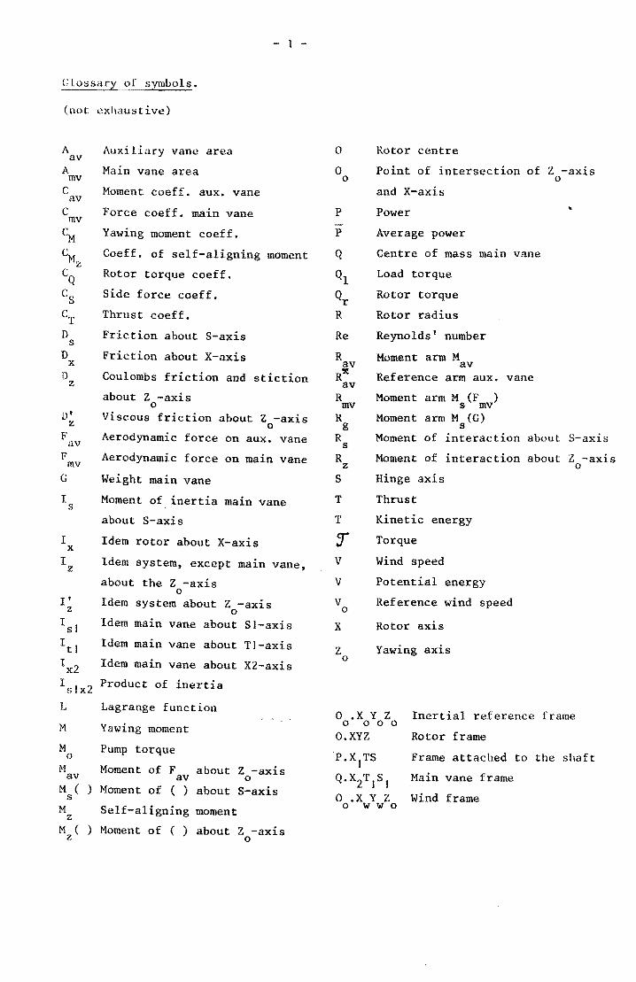
GLossary of synlbols.
(not exhaustive)
A av
A mv C av C mv eM c Mz C
Q Cs CT D
s D
x D
z
0' z
F av F
mv G
I s
I x
I z
I I
z
Is)
Itl
Ix2
Islx2
L
M
M o
M av M ( )
s M
z M ( )
z
Auxiliary vane area
Main vane area
Moment coeff. aux. vane
Force coeff. main vane
Yawing moment coeff.
Coeff. of self-aligning moment
Rotor torque coeff.
Side force coeff.
Thrust coeff.
Friction about S-axis
Friction about X-axis
Coulombs friction and stiction
about Z-axis o
Viscous friction about Z-axis o
Aerodynamic force on aux. vane
Aerodynamic force on main vane
Weight main vane
Moment of inertia main vane
about S-axis
Idem rotor about X-axis
Idem system, except main vane,
about the Z-axis o
Idem system about Z-axis o
Idem main vane about S)-axis
Idem main vane about TI-axis
Idem main vane about X2-axis
Product of inertia
Lagrange function
Yawing moment
Pump torque
Moment of F about Z-axis av 0
Moment of ( ) about S-axis
Self-aligning moment
Moment of ( ) about Z-axis 0
o o o
Re
R av RX
av R mv
R
R
R
S
T
T
v V
V
g
s
z
o
x
z o
Rotor centre
Point of intersection of Z-axis o
and X-axis
Power
Average power
Centre of mass main vane
Load torque
Rotor torque
Rotor radius
Reynolds' number
Moment arm M av Reference arm aux. vane
Moment arm M (F ) s mv
Moment arm M (G) s
Moment of interaction about S-axis
Moment of interaction about Z-axis o
Hinge axis
Thrust
Kinetic energy
Torque
Wind speed
Potential energy
Reference wind speed
Rotor axis
Yawing axis
0 .X Y Z Inertial reference frame 0 000
O.XYZ Rotor frame
P.X)TS Frame attached to the shaft
Q.X2TIS1 Main vane frame
0 .X Y Z Wind frame 0 w w 0
a
c
d x
d s
d z
f
g
h mv h
g m
t ~
B
y
6 o
p
D o
(J
T X
T S
T Z
~mv
- 2 -
Axial interference factor
Blade chord
Friction parameter
Friction parameter
Friction parameter
Distance rotor plane Z-axis 0
Gravitational acceleration
See page 7
See page 7
Mass main vane
Dimensionless time variable
Friction parameter Z-axis o
Interpolation factor
Load parameter
position angle main vane
Projection of y on x Y plane o 0
Preset angle main vane
Initial value of y
position angle shaft
Yawing angle
Initial value of ,
Angle between Sand Z-axis o
Idem but in case ~ I 0
See page 49
Tip speed ratio
Optimum tip speed ratio
Kinematic viscosity of air
Preset angle aux. vane
Air density
Air density at standard P, T
Scale factor
Time constant X-axis
Time constant S-axis
Time constant Z-axis o
Angle between X -axis and proo
jection of vane arm on X Y -o 0
plane
~ Angle of attack main tPmv vane
X Wind direction w
Main vane's inertial angular
speed
11 Angular speed rotor
11 Dimensionless angular speed ~
-3-
! General introduction
In rural areas in most developing countries there is a strong urge for water
for both human as well as agricultural needs. Among others wind energy systems
are employed for this purpose. Cost aspects and the availability of materials
account for the interest in purely mechanical wind energy systems.
To avoid damage caused by high wind speeds, control systems are utilized,
whose control properties ought to meet the following demands:
i. limitation of the rotor's angular speed to protect rotor, trans
fer system and load
ii. avoidance of oscillatory behaviour to prevent the occurence of
excessive forces and torques
One of the current control systems is the so-called inclined hinged vane con
trol system with auxiliary vane.
Closely related are control systems in which the function of the auxiliary
vane is replaced by rotor excentricity or in which the inclined hinge is re
placed by a spring providing the retarding moment.
Although under stationary conditions the behaviour of a wind energy system
utilizing an inclined hinged vane control system turns out to be predictable,
its field performance gives rise to several questions.
The aim of this survey was to develop a mathematical model for this system
and to develop a computer program to enable continuous simulation.
Furthermore wind tunnel tests on a scale model were carried out to determine
the nature of the aerodynamic forces and torques acting on its component parts.
In chapter II a mathematical model is set up for the first above mentioned
sytem. Besides this chapter contains a section in which the system different
ial equations, constituting the mathematical model, are put into dimension
less form, followed by an attempt to investigate scaling problems.
It ends with an approach in terms of input-output relations.
Chapter III deals with the computer simulation of physical models. It intro
duces the interactive simulation language THTSIM. Finally it presents the
outline of a computerprogram for simulation of the system in question.
Chapter IV presents a detailed description of the computer program and some
results.
In chapter V the results of wind tunnel tests are presented. Furthermore it
contains a discussion on the agreement of results of both computer program
and wind tunnel tests.

-4-
Finally, chapter VI contains an evaluation on the results.
The reader is kindly requested to accept our apologies for any abuse of
english grammar and language, that might occur in this report.
- 5 -
II Theory
2.1 Introduction
In this chapter a mathematical model is set up that will be employed to
simulate the system's dynamic behaviour.
With 'the system', rotor, shaft and both vanes will be meant. The system
boundary secludes the system from its surroundings to which all other wind
turbine parts, as well as the air flow and the load belong.
The system is acted upon by a number of forces and torques exerted by its
surroundings. According to their nature, they can be divided into three
groups:
i. aerodynamic
ii. gravitational
iii. dissipative forces and torques
Obviously, the surroundings in their turn.are affected by the system.
The system is one with three rotational degrees of freedom, its :dynamic
behaviour including rotational motion of
- the rotor about its own axis
- the shaft about the yawing axis
- the main vane about its inclined hinge axis
As a consequence the model consists of three differential equations apart
from a number of supplementary relationships. These differential equations
will turn out to be coupled and non-linear.
Before deriving them, system geometry and the coordinate systems used for
the description of its behaviour, are dealt with in section 2.2.
In sections 2.3 and 2.4 the above mentioned forces and torques will be dis
cussed in detail.
Except for rotor motion about its own axis, for which the differential equa
tion is set up in a straightforward way, the equations that constitute the
model will be derived by means of Langrange's equations (section 2.5).
In section 2.6 a general discussion of preset angles is given.
Section 2.7 is meant to give an overview of the model equations.
In section 2.8 the model equations will be put into dimensionless form, thus
extending their validity considerably.
Finally, in section 2.9 a system analytical approach is made.
- 6 -
2.2 System geometry and coordinate systems
2.2.1 Introduction
This section will be concerned with system geometry (2.2.2) and the coor-
dinate systems used in describing the system's behaviour (2.2.3).
The main vane is assumed to have no preset angle in order to avoid unneces
sary complications in deriving the equations of motion. A general discussion
of preset angles is given in section 2.6.
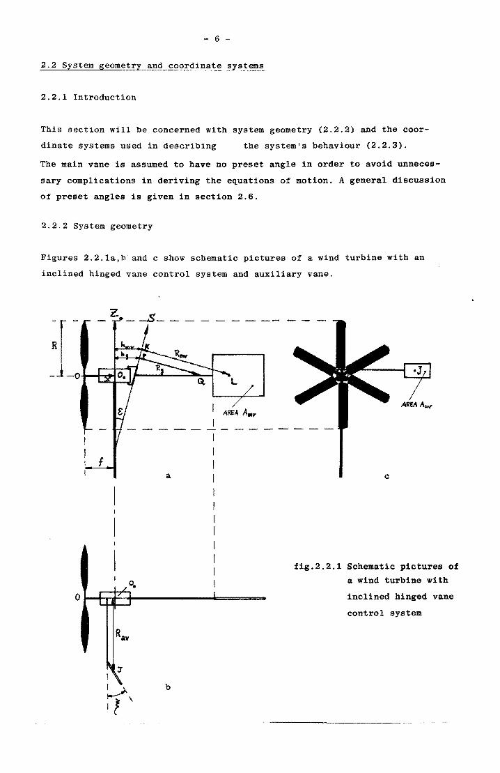
2.2 2 System geometry
Figures 2.2.1a,p and c show schematic pictures of a wind turbine with an
inclined hinged vane control system and auxiliary vane.
R
f
/0.
0 I -. I
RAY
~ :r 1
~\
a
b
I I I I I I I I I I I I
c
fig.2.2.1 Schematic pictures of
a wind turbine with
inclined hinged vane
control system
- 7 -
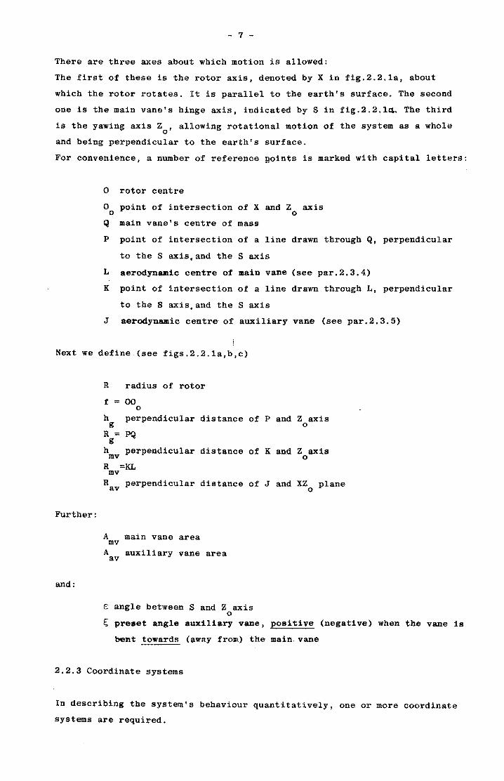
There are three axes about which motion is allowed:
The first of these is the rotor axis, denoted by X in fig.2.2.1a, about
which the rotor rotates. It is parallel to the earth's surface. The second
one is the main vane's hinge axis, indicated by S in fig.2.2.1~. The third
is the yawing axis Z , allowing rotational motion of the system as a whole o
and being perpendicular to the earth's surface.
For convenience, a number of reference Roints is marked with capital letters:
o rotor centre
o point of intersection of X and Z axis o 0
Q main vane's centre of mass
P pOint of intersection of a line drawn through Q, perpendicular
to the S axis,and the Saxis
L aerodynamic centre of main vane (see par.2.3.4)
K point of intersection of a line drawn through L, perpendicular
to the S axis. and the Saxis
J aerodynamic centre of auxiliary vane (see par.2.3.5)
Next we define (see figs.2.2.1a,b,c)
Further:
and:
R radius of rotor
f = 00 o
h g perpendicular distance of P and Z axis
o R = PQ
g h perpendicular distance of K and Z axis
mv 0
R =KL mv
R perpendicular distance of J and XZ plane av 0
A main vane area mv A auxiliary vane area av
s angle between Sand Z axis o
~ pre.et angle auxiliary vane, positive (negative) when the vane is
bent towards (away from) the main vane
2.2.3 Coordinate systems
In describing the system's behaviour quantitatively. one or more coordinate
systems are required.
- 8 -
It is of great importance to have clear agreements about the coordinate
sytems to be used.
They will all be right-handed systems having an orthonormal set of base
vectors. Coordinate axes will be denoted by capital letters (e.g. X,Y,Z).
Small letters will be used to indicate the corresponding unit vectors.
In order to emphasize their vector character, they are accompanied with'
a small dash below them (e.g. !.,x..,~), as will all other vector quantities
in later sections. Small letters only (e.g. x,y,z), will denote coordinates.
We now consider the X, S and Z axis of the previous paragraph to be coordio
nate axes of coordinate systems to be defined below.
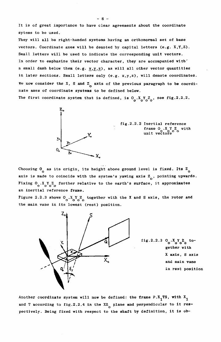
The first coordinate system that is defined, is 0 .X Y Z , see fig.2.2.2. o 000
x.
fig.2.2.2 Inertial reference frame 0 .X Y Z with unit vegto~so 0
Choosing 0 as its origin, its height above ground level is fixed. Its Z o 0
axis is made to coincide with the system's yawing axis Z , pointing upwards. o
Fixing 0 .X Y Z fUrther relative to the earth's surface, it approximates o 000
an inertial reference frame.
Figure 2.2.3 shows 0 .X Y Z together with the X and S axis, the rotor and o 000
the main vane in its lowest (rest) position.
fig.2.2.3 0 .X Y Z too 000
gether with
X axIs, Saxis
and main vane
in rest position
Another coordinate system will now be defined: the frame P.X1TS, with Xl
and T according to fig.2.2.4 in the XZ plane and perpendicular to it reso
pectively. Being fixed with respect to the shaft by definition, it is ob-
- 9 -
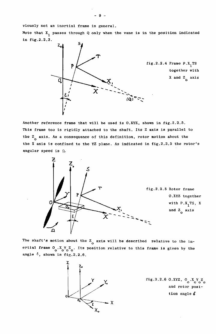
viously not an inertial frame in general.
Note that Xl passes through Q only when the vane is in the position indicated
in fig.2.2.3.
fig.2.2.4 Frame P.XITS
together with
X and Z axis o
Another reference frame that will be used is O.XYZ, shown in fig.2.2.5.
This frame too is rigidly attacbed to the shaft, Its Z axis is parallel to
the Z axis. As a consequence of this definit~on. rotor motion about the o
the X axis is confined to the YZ plane. As indicated in fig.2.2,5 the rotor's
angular speed is n.
l • s
fig.2.2.5 Rotor frame
O.XYZ together
with P. Xl TS, X
and Z axis o
The shaft's motion about the Z axis will be described relative to the In-. 0
ertial frame 0 .X Y Z . Its position relative to this frame is given by the o 000
angle 0, shown in fig.2.2.6.
2. l ..
x
fig.2.2.6 O.XYZ, 0 .X Y Z o 000
and rotor posi-
tion angle 6
- 10 -
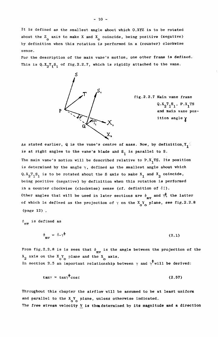
It is defined as the smallest angle about which O.XYZ is to be rotated
about the Z axis to make X and X coincide, being positive (negative) o 0
by definition when this rotation is performed in a (counter) clockwise
sense.
For the description of the main vane's motion, one qther frame is defined.
This is Q.X2
T1
S1
of fig.2.2.7, which is rigidly attached to the vane.
s
p
fig.2.2.7 Main vane frame
Q.X2T1S1
, P.X1
T8
and main vane pos-
i tion angle 'K
As stated earlier, Q is the vane's centre of mass. Now, by definition.T1
is at right angles to the vane's blade and 81
is parallel to S.
The main vane's motion will be described relative to P.X1TS. Its position
is determined by the angle y, defined as the smallest angle about which
Q.X2T1S1 is to be rotated about the S axis to make Xl and X2 coincide,
being positive (negative) by definition when this rotation is performed
in a counter clockwise (clockwise) sense (cf. definition of o!).
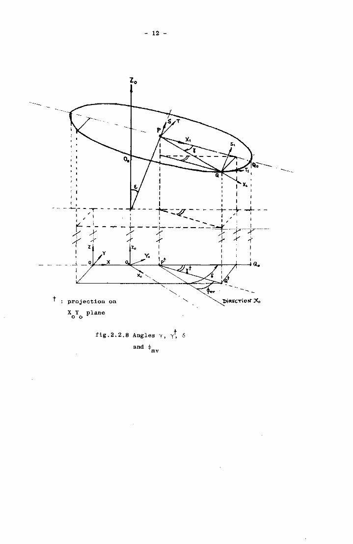
Other angles that will be used in later sections are ¢ and y~ the latter mv
of which is defined as the projection of y on the X Y plane, see fig.2.2.8 o 0
(page 12) •
$ is defined as mv
(2.1)
From fig.2.2.8 is is seen that ¢ is the angle between the projection of the mv
X2 axis on the X Y plane and the X axis. 000
In section 2.5 an important relationship between y and ytWil1 be derived:
tany tany+cosE: (2.57)
Throughout this chapter the airflow will be assumed to be at least uniform
and parallel to the X Y plane, unless otherwise indicated. o 0
The free stream velocity! is thea determined by its magnitude and a direction
- 11 -
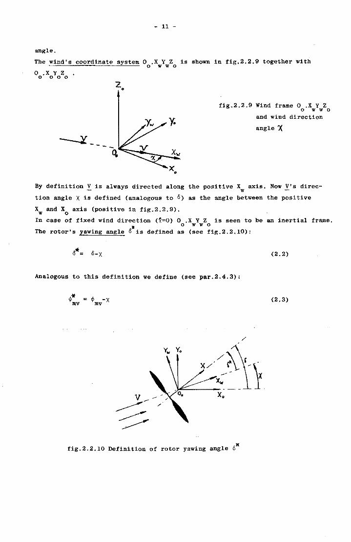
angle.
The windts coordinate system 0 .X Y Z is shown in fig.2.2.9 together with o w w 0
o .X Y Z o 000
Z II
fig.2.2.9 Wind frame 0 .X Y Z o w w 0
y. and wind direction
angle ?(
x.
By definition V is always directed along the positive X axis. Now Vts direcw
tion angle X is defined (analogous to 0) as the angle between the positive
X and X axis (positive in fig.2.2.9). w 0
In case of fixed wind direction (~=O) 0 .X Y Z is seen to be an inertial frame. " 0 w w 0
The rotorts yawing angle 0 is defined as (see fig.2.2.10):
0·= o-x
Analogous to this definition we define (see par.2.4.3):
cj>~ = If> -X mv mv
J(
fig.2.2.10 Definition of rotor yawing angle 0
/'
(2.2)
(2.3)
---
t
- 12 -
, .
, I
projection on
X Y plane o 0
fig.2.2.8 Angles y, y~ 8
and 4> mv
--
- 13 -
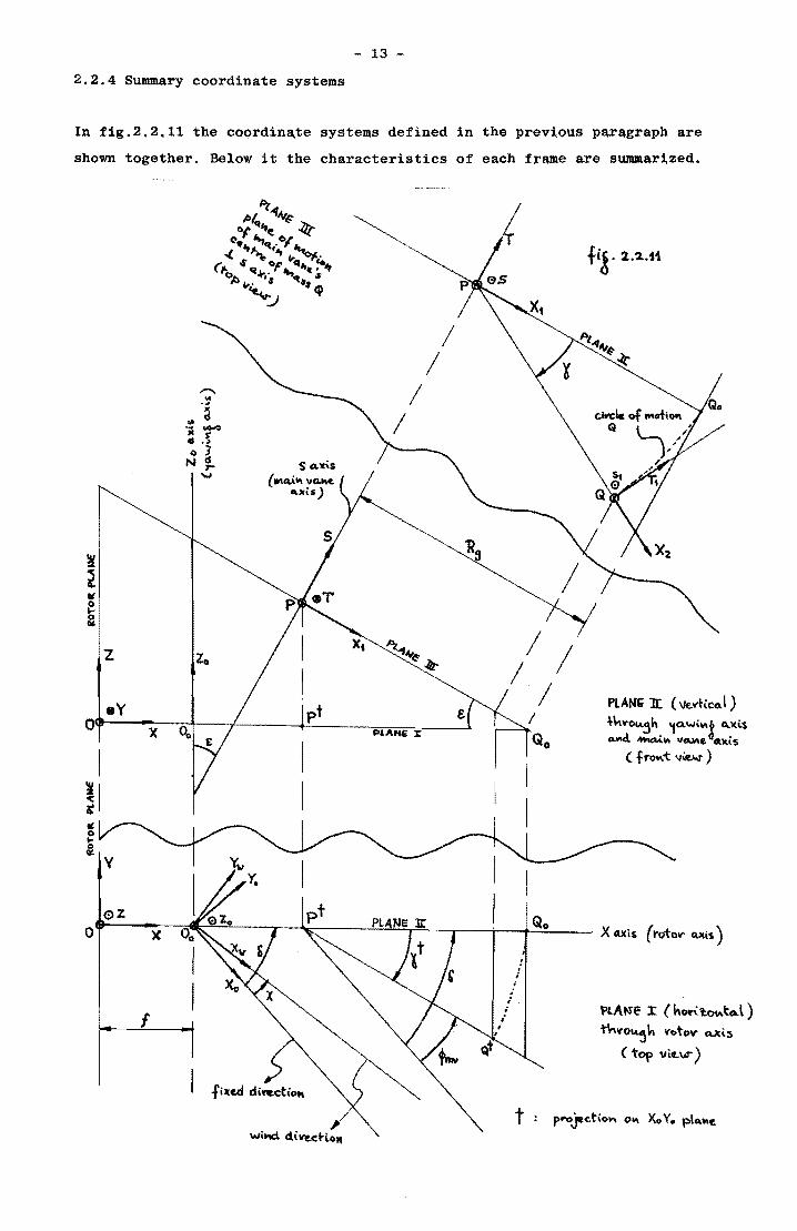
2.2.4 Summary coordinate systems
In fig.2.2.11 the cOQrdin~te systems defined in the PreviQus paragraph are
shown together. Below it the characteristics of each fr~e are summarized.
~ t " i
z ZO
.Y 0 X
II t Ii: 0 t-o CIt
f
/
/ /
/
PLAtt .. x
/ / / /
! i
i , ,..
PlAf{& lI: (\le.vt~cQ. \ ) -\-~you.~h '1Q.Wi.IiI~ D..l(i.$
CLoo4 ~1iI v_e. ()Q.lC.t5
( frolll.t \f\le.l.r )
~lAN"e ::t (hcw\'tcIllt:Cl.l) ~V'o~ k yotov cu:;i.:s
(top vi~W")
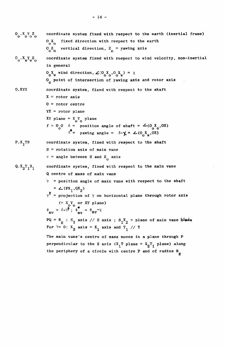
o .X Y Z o 000
o .X Y Z o w w 0
O.XYZ
- 14 -
coordinate system fixed with respect to the earth (inertial frame)
o X fixed direction with respect to the earth o 0
o Z vertical direction, Z = yaw.ing axis 000
coordinate system fixed with respect to wind velocity, non-inertial
in general
o X wind direction, ..!~O X ,0 X ) = X o woo 0 w
o point of intersection of yawing axis and rotor axis o
coordinate system, fixed with respect to the shaft
X = rotor axis
o = rotor centre
YZ = rotor plane
XY plane = X Y plane o 0
f = 0 0 o
o = 0*=
position angle of shaft = ~(O X ,OX) o 0
yawing angle = 0--.1 = ~(O X ,OX) ,. ow
coordinate system, fixed with respect to the shaft
S = rotation axis of main vane
£ = angle between Sand Z axis o
coordinate system, fixed with respect to the main vane
Q centre of mass of main vane
y = position angle of main vane with respect to the shaft
= '-- (PX1
,QX2
)
yt = projection of y on horizontal plane through rotor axis
(= X Y or XY plane) 00* = o_yt. ~ = '" -X , mv "'mv ~ mv
PO = R • g 81 axis II 8 axis; S1X2 = plane of main vane bt8de For y= 0: X2 axis = Xl axis and Tl II T
The main vane's centre of mass moves in a plane through P
perpendicular to the Saxis (X1
T plane = X2Tl plane) along
the periphery of a circle with centre P and of radius R g
- 15 -
2.3 Aerodynamic forces and torques
2.3.1 Introduction
This section will be concerned with the aerodynamic
and torques to which the system is subjected.
part of the forces
Forces and torques on rotors are dealt with below (2.3.2).
As an introduction to and a special case of main vane (2.3.4) and auxiliary
vane aerodynamics (2.3.5), vane behaviour in uniform flow is viewed in 2.3.3.
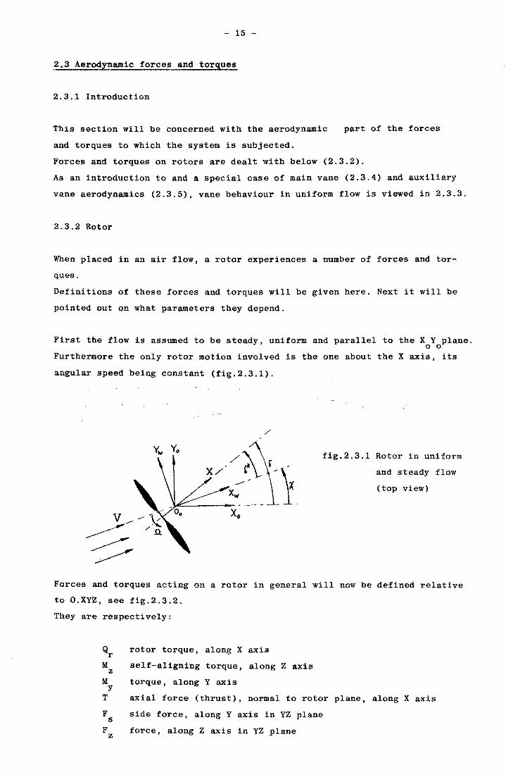
2.3.2 Rotor
When placed in an air flow, a rotor experiences a number of forces and tor
ques.
Definitions of these forces and torques will be given here. Next it will be
pointed out on what parameters they depend.
First the flow is assumed to be steady, uniform and parallel to the X Y plane. o 0
Furthermore the only rotor motion involved is the one about the X axis, its
angular speed being constant (fig.2.3.1).
/
fig.2.3.1 Rotor in uniform
and steady flow
(top view)
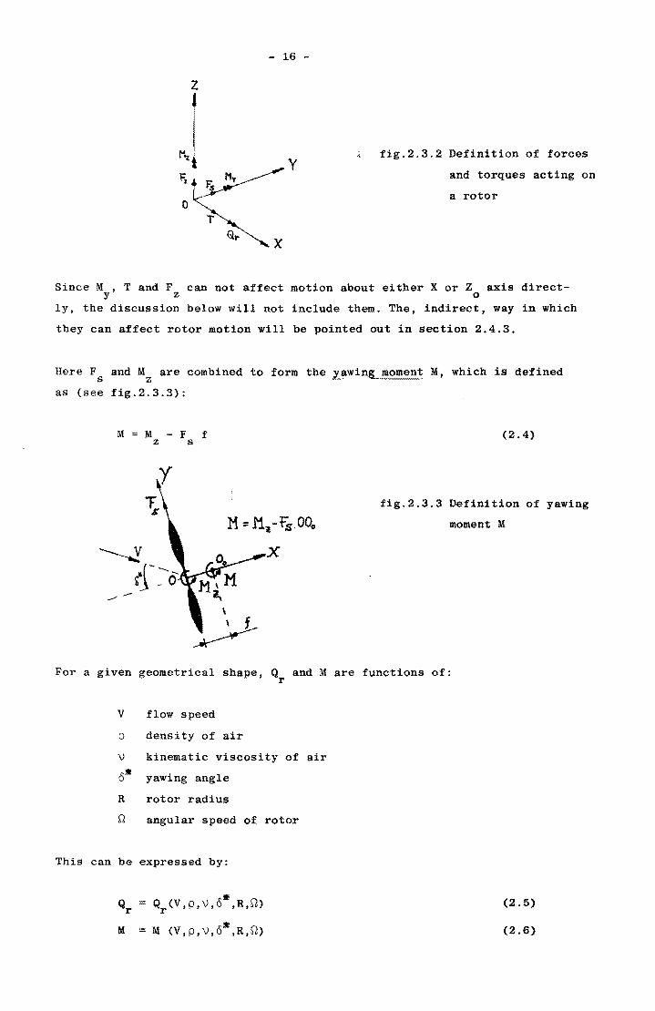
Forces and torques acting on a rotor in general will now be defined relative
to O.XYZ, see fig.2.3.2.
They are respectively:
Qr rotor torque, along X axis
M self-aligning torque, along Z axis z M torque, along Y axis y T axial force (thrust), normal to rotor plane, along X axis
F side force, along Y axis in YZ plane s F force, along Z axis in YZ plane z
z
o T
- 16 -
x
fig.2.3.2 Definition of forces
and torques acting on
a rotor
Since M , T and F can not affect motion about either X or Z axis direct-y Z 0
ly, the discussion below will not include them. The, indirect, way in which
they can affect rotor motion will be pointed out in section 2.4.3.
Here Fs and Mz
are combined to form the yawing moment M, which is defined
as (see fig.2.3.3):
M M z
F f s
\ \ f ~
(2.4)
fig.2.3.3 Definition of yawing
moment M
For a given geometrical shape, Q and M are functions of: r
V flow speed
p density of air
\! kinematic viscosity of air
o· yawing angle
R rotor radius
Q angular speed of rotor
This can be expressed by:
J! Qr(V,P,\!,O ,R,Q) (2.5)
J! = M (V,p,V,o ,R,Q) (2.6)
- 17 -
Applying Buckingham's IT-theorem, the following dimensionless groups of
parameters can be formed:
CQ
Qr = 2. 3 lpy TIR (rotor) torque coefficient
CM M =
iOV2TIR3
yawing moment coefficient
A QR
=-V
tip-speed ratio
0· yawing angle
Re VR =-
'J Reynolds' number
Relations (2.5) and (2.6) transform into:
• = CQ(A,O ,Re)
• CM(A,O ,Re)
(2.7)
(2.8)
(2.9)
(2.2)
(2.10)
(2.11)
(2.12)
As lift and drag characteristics hardly depend on Re for a slow-running
rotor's blade profile, (2.11) and (2.12) can be written as:
(2.13)
(2.14)
NOTE that, if steady flow is assumed, one may put x=O without loss of
generality. In that case the yawing angle o· equals 0 (see CHAPTER V).
In Ittl theoretical CQ
, Cs ~see definition (2.15» 'SxidCT(thrust coefficient,
defined in a way similar to Cs) can be found.
This is done for a 16-bladed wind turbine by means of a simple theoretical
model. According to 1131 this so-called classical model can not account for
the self-aligning moment M . z
Experimental work has been done by the authors of 141, 1,,'1, 1.'1 and 1131, concerning C
Q only.
In CHAPTER V other wind tunnel tests on slow-running rotors will be present
ed. These tests concern the yawing moment.
From fig.2.3.3 it can be seen that the aligning behaviour of a rotor (re
lated to both F and M ; aligning: tendency to decrease 0·) strongly de-s z
- 18 -
pends on the value of f.
In 101 it is stated that for slow-running wind turbines this aligning be
haviour is less pronounced than for fast-running wind turbines, probably
being due to a difference in side force.
In 1,1 the effects of non-uniform and non-axial flow (8*rO) on forces and
* torques are investigated, the latter being valid for small 8 only.
It should be emphasized that for CM
to be equal for two turbines of differ
ent size, mere geometrical similitude of their rotors is not sufficient.
They should have the same fiR ratio too, as will become clear from the fol
lowing.
Defining the rotor's side force coefficient CSand self-aligning torque coef
ficient CM by: z
M C = z
Mz .1 V2 R3 2P 'IT
(2.15)
(2.16)
Cs and CMz
' like CQ
and CM' turn out to be functions of A and a*. Using (2.8), (2.15) and (2.16), (2.4) can be written as:
(2.17)
• • Now, for two rotors of equal geometrical shape, both CM
(A,a ) and CS(A,Q ) z
are equal. For CM
to be equal for both turbines, fiR should be equal, as
can be seen from (2.17). In fact this is ordinary geometrical similitude of
the two turbines, concerning relevant dimensions.
Allowing Q, V and X to be functions of time, the following assumption is
made.
The aerodynamic flow around the blades is steady. This means that it needs
much less time to adjust itself to changes in wind velocity (i.e. V and X)
than the rotor's angular speed Q does,
Further the effects of a non-zero (inertial) angular velocity 0 on Q and r
M are neglected, assuming 0 to be sufficiently small.
Their evaluation would, in essence, require knowledge of how a non-uniform
- 19 -
disturbance velocity field affects the forces and torques acting on a
rotor.
The last assumption that is made is that Q and M are in no way affected r
by the presence of the vanes and the shaft,
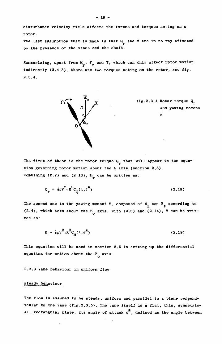
Summarizing, apart from M ,F and T, which can only affect rotor motion y z
indirectly (2.4.3), there are two torques acting on the rotor, see fig.
2.3.4.
fig.2.3.4 Rotor torque Q r
and yawing moment
M
The first of these is the rotor torque Q that wrIl appear in the equa-r
tion governing rotor motion about the X axis (section 2.5).
Combining (2.7) and (2.13), Q can be written as: r
The second one is the yawing moment M, composed of M and F according to z s
(2.4), which acts about the Z axis. With (2.8) and (2.14), M can be writo
ten as:
(2.19)
This equation will be used in section 2.5 in setting up the differential
equation for motion about the Z axis. o
2.3.3 Vane behaviour in uniform flow
steady behaviour
The flow is assumed to be steady, uniform and parallel to a plane perpend
icular to the vane (fig.2.3.5). The vane itself is a flat, thin, symmetric
• aI, rectangular plate. Its angle of attack ~ , defined as the angle between
- 20 -
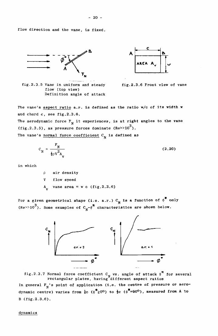
flow direction and the vane, is fixed.
___ : --¢·V~ ----.... f\_
"FN
fig.2.3.5 Vane in uniform and steady flow (top view) Definition angle of attack
c A ~
AREA Av
fig.2.3.6 Front view of vane
The vane's aspect ratio a.r. is defined as the ratio w/c of its width w
and chord c, see fig.2.3.6.
The aerodynamic force FN it experiences, is at right angles to the vane 3
(fig.2.3.5), as pressure forces dominate (Re»10 ).
The vane's normal force coefficient CN
is defined as
(2.20)
in which
p air density
V flow speed
A vane area = w c (fig.2.3.6) v
• For a given geometrical shape (i.e. a.r.) CN
is a function of ~ only
(Re»103). Some examples of CN-~· characteristics are shown below.
elll
1
If
---- '1>
-----Q.t': • 1
., ---- ¢
fig.2.3.7 Normal force coefficient C vs. angle of attack ~K for several rectangular plates, havingNdifferent aspect ratios
In general FN's point of application (i.e. the centre of pressure or aero-
dynamic centre) varies from ic (~·~Oo) to tc (~·=900), measured from A to
B (fig.2.3.6).
- 21 -
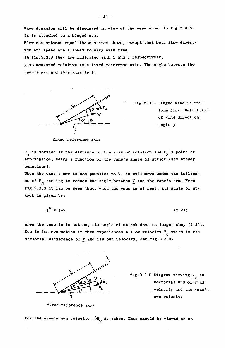
Vano dynamics will be discu.sed in viow of the vane shown in f11. 2 •3 •8 •
It is attached to a hinged arm.
Flow assumptions equal those stated above, except that both flow direct
ion and speed are allowed to vary with time.
In fig.2.3.8 they are indicated with X and V respectively.
X is measured relative to a fixed reference axis. The angle between the
vane's arm and this axis is $.
fixed reference axis
fig.2.3.8 Hinged vane in uni
form flow. Definition
of wind direction
angle X
Rv is defined as the distance of the axis of rotation and FN'S point of
application, being a function of the vane's angle of attack (see steady
behaviour).
When the vane's arm is not parallel to !, it will move under the influen
ce of FN tending to reduce the angle between! and the vane's arm. From
fig.2.3.8 it can be seen that, when the vane is at rest, its angle of at
tack is given by:
$- = $-X (2.21)
When the vane is in motion, its angle of attack does no longer obey (2.21).
Due to its own motion it then experiences a flow velocity V which is the -c
vectorial difference of V and its own velocity, see fig.2.3.9.
fixed reference axis
fig.2.3.9 Diagram showing V as -c
vectorial sum of wind
velocity and the vane's
own velocity
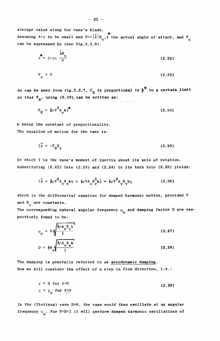
For the vane's own velocity. ~R is taken. This should be viewed as an v
- 22 -
average value along the vane's blade.
Assuming ~-X to be small and V»I~'R ,~the actual angle of attack, and V v c
can be expressed by (see fig.2.3.9):
v '" V c
(2.22)
(2.23)
. '
As can be seen from fig.2.3.7, eN is proportional to ~ to a certain limit
so that FN, using (2.22), can be written as:
k being the constant of proportionality.
The equation of motion for the vane is:
.. 14> = -F R N v
(2.24)
(2.25)
in which I is the vane's moment of inertia about its axis of rotation.
Substituting (2.22) into (2.24) and (2.24) in its turn into (2.25) yields:
(2.26)
which is the differential equation for damped harmonic motion, provided V
and R are constants. v
The corresponding natural angular frequency 000
and damping factor D are res-
pectively found to be:
00 o
D
JiPA R k' V v v I
The damping is generally referred to as aerodynamic damping.
(2.27)
(2.28)
Now we will consider the effect of a step in flow direction, i.e.:
x = 0 for t<O
X = X for t"O o
(2.29)
In the (fictious) case D=O, the vane would then oscillate at an angular
frequency w . For O<D<l it will perform damped harmonic oscillations of o
frequency w':
w' = w ft_D2' o
- 23 -
(2.30)
Measurements performed by Der Kinderen and Van Meel 191 on a vane's oscilla
tory behaviour show a good agreement with theory.
When 0=1, vane motion is critically damped, while for D>l it is overdamped.
Note that w' increases with wind speed V and that D is independent of V.
For most vanes D turns out to be small «.25), implying wt~w • however desio
rable it would be to have critically damped or overdamped vanes.
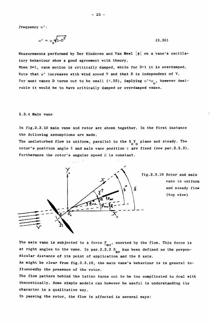
2.3.4 Main vane
In fig.2.3.10 main vane and rotor are shown together. In the first instance
the following assumptions are made.
The undisturbed flow is uniform, parallel to the X Y plane and steady. The o 0
rotor's position angle 0 and main vane position yare fixed (see par.2.2.3).
Furthermore the rotor's angular speed n is constant.
fig.2.3.10 Rotor and main
-=-----
vane in uniform
and steady flow
(top view)
The main vane is subjected to a force F ,exerted by the flow. This force is -mv
at right angles to the vane. In par.2.2.2 R has been defined as the perpen-mv
dicular distance of its point of application and the Saxis.
As might be clear from fig.2.3.10, the main vane's behaviour is in general in
fluencedby the presence of the rotor.
The flow pattern behind the latter turns out to be too complicated to deal with
theoretically. Some Simple models can however be useful in understanding its
character in a qualitative way.
In passing the rotor, the flow is affected in several ways:
- 24 -
As energy is extracted in general from the flow by the rotor, the flow's
speed in the rotor's wake will be less than V. According to momentum theo
ry 191 it is about one third of the original flow speed, when !=O and maxi
mum power is extracted from the flow.
From Newton's third law it follows that it is rotational too in general,
its angular velocity and the rotor's angular velocity having opposite signs.
For slow-running wind turbines this wake rotation turns out to be greater
than for fast-running wind turbines. This is due to a difference in rotor
torque CQ
' this torque being relatively high for slow-running turbines.
In general, flow direction is affected too. A simple model might account for
this deflection: In exerting a side force !S on the rotor (see par.2.3.2),
the flow experiences, again by Newton's third law, in its turn a force -!S' causing its direction to change.
Furthermore, the flow possesses vorticity, originating at the rotor.
Summarizing, in general the flow near the vane is far from uniform.
For a given geometrical shape F is a function of: mv
any characteristic length
V - flow speed
p - mass density of air
n - angular speed of rotor
• o - yawing angle
• ~mv - see fig.2.3.10 and par.2.2.3
The main vane's dimensionless force coefficient C is defined as: mv
C = mv
F mv
in which A is the vane's area. mv _
C is then found to be some function Of~· 0 and A mv mv'
~ . C = C ($ ,o,A) mv mv mv
(2.31)
(2.32)
It is important to note that definition (2.31) is not equivalent to (2.20)
unless the flOW, the vane is in, is uniform, parallel to the X2T1 plane (in
dependent of y), steady and its speed equals V, which is never the case.
C mv would then, like CN' be a function of the angle of attack alone.
For a non-inclined vane (£=0) wind tunnel tests concerning (2.32) have been
carried out 12tl. A brief discussion of them can be found in par.5.3.2.1.
~. 25 -
When the vane is in motion with respect to the shaft (YrO) , F is also mV
a function of y (or ~ when &=0), causing the vane to be aerodynamically mv
damped (cf. par.2.3.3 'dynamics').
Defining the vane's speed-ratio:
11=
and maintaining definition (2.31) for C ,(2.32) should then be changed mv
into the more general form:
.. * C· = C (t ,5,~,1l) mv mv mv (2.34)
It is however hardly possible to determine this functional form experiment
ally.
In order to take account of the vane's own motion all the same, a number of
simplifications is made at this pOint.
... . + C is a function of cp and 0 only
mv mv
it '* C = C (cp ,0) mv mv mv
(2.35)
+ The flow behind the rotor is uniform and steady, regardless the value .. of O.
+ Flow direction is not affected by the rotor. In other words, the flow
1s not deflected.
+ When at rest, the vane's angle of attack equals (cf.(2.21»
(2.3)
+ To take account of the vane's own motion, the vane's angle of attack • • is written as (cf.(2.22»: mv
'* <Pmv (2.36)
The factor (I-a) in the last term is introduced to express that flow
speed behind the rotor is only a fraction of the original flow speed
V. It is given a constant value of 1/3 in that term, which is the ap-• proximate value when 0=0 and maximum power is extracted from the flow
(see par.2.3.3 'dynamics')
3$ R ;; A. mv mv
'i'mv-X+ V (2.37)
- 26 -
Using (2.31) and (2.35), F can now be written as: mv
F mv
2 it tI = !pV A C (¢ ,0) mv mv mv (2.38)
When ~, V, X, ¢:v and a*are also allowed to be functions of time, (2.37) and
(2.38) are assumed still to be valid without any further notice.
Furthermore it is assumed that the main vane's behaviour is not affected by
the auxiliary vane.
It is important to note that as a consequence of the first assumption above,
any change of wind velocity will arrive simultaneously at the rotor and the
main vane. More attention to this phenomenon will be paid in par. ~.~ .
Equation (2.38), completed with (2.37) and (2.2) will be used in setting up
the differential equations governing motion about Sand Z axis (section 2.5). o
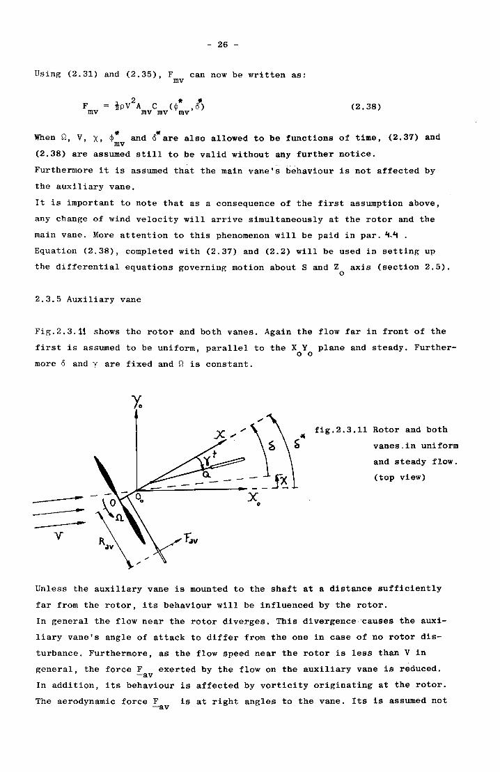
2.3.5 Auxiliary vane
Fig.2.3.11 shows the rotor and both vanes. Again the flow far in front of the
first is assumed to be uniform, parallel to the X Y plane and steady. Furthero 0
more 0 and yare fixed and ~ is constant.
"
-")~~
~-=~-----X
o
--y
fig.2.3.11 Rotor and both
vanes. in uniform
and steady flow.
(top view)
Unless the auxiliary vane is mounted to the shaft at a distance sufficiently
far from the rotor, its behaviour will be influenced by the rotor.
In general the flow near the rotor diverges. This divergence, :causes the auxi
liary vane's angle of attack to differ from the one in case of no rotor dis
turbance. Furthermore, as the flow speed near the rotor is less than V in
general, the force F exerted by the flow on the auxiliary vane is reduced. -av
In addition, its behaviour is affected by vorticity originating at the rotor.
The aerodynamic force F is at right angles to the vane. Its is assumed not -av
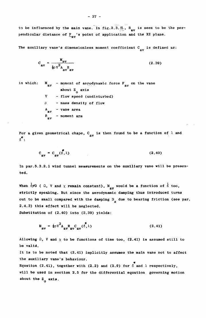
- 27 -
to be influenced by the main vane. In fig.2.3.j1., R is seen to be the perav
pendicular distance of F 's point of application and the XZ plane. -av
The auxiliary vane's dimensionless moment coefficient C is defined as: av
C av
= Mav iPV2A--R
av av
(2.39)
in which: M - moment of aerodynamic force F on the vane av av about Z axis
o V - flow speed (undisturbed)
p - mass density of flow
A - vane area av R - moment arm
av
For a given geometrical chape, C is then found to be a function of A and av
0"':
* C = C (o,A) av av (2.40)
In par.5.3.2.l wind tunnel measurements on the auxiliary vane will be presen
ted.
. . When o~O ( n, V and X remain constant), M would be a function of 0 too,
av strictly speaking. But since the aerodynamic damping thus introduced turns
out to be small compared with the damping D due to bearing friction (see par. z
2.4.3) this effect will be neglected.
Substitution of (2.40) into (2.39) yields:
(2.41)
Allowing n, V and X to be functions of time too, (2.41) is assumed still to
be valid.
It is to be noted that (2.41) implicitly assumes the main vane not to affect
the auxiliary vane's behaviour.
* Equation (2.41), together with (2.2) and (2.9) for 0 and A respectively,
will be used in section 2.5 for the differential equation governing motion
about the Z axis. o
- 28 -
2.4 Forces and moments of other nature
2.4.1 Introduction
Apart from aerodynamic forces and moments, the system is subjected to forces
and moments of other nature.
Below in par.2.4.2 the force of gravity on the main vane is viewed.
Par.2.4.3 deals with the dissipative moments acting on the system.
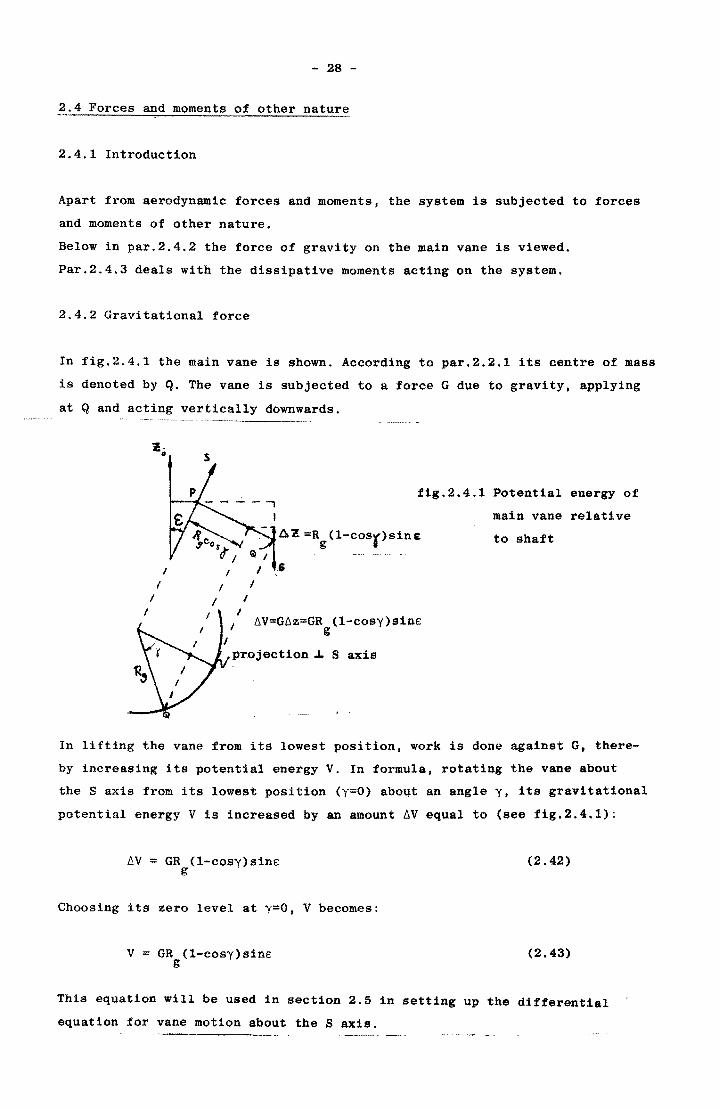
2.4.2 Gravitational force
In fig.2.4.1 the main vane is shown. According to par.2.2.1 its centre of mass
is denoted by Q. The vane is subjected to a force G due to gravity, applying
at Q and acting vertically downwards.
~-II .s
--, I
fig.2.4.1 Potential energy of
main vane relative
I
I I
I
I I
I
I
I
I
I I
I
.o.z =Rg (l-coSr)Sine
G
I 6V=G6z=GR (l-cosy)sinE g
projection.J. Saxis
to shaft
In lifting the vane from its lowest position, work is done against G, there
by increasing its potential energy V. In formula, rotating the vane about
the S axis from its lowest position (y=O) about an angle y, its gravitational
potential energy V is increased by an amount 6V equal to (see fig.2.4.1):
~V = GR (l-cosy)sinE g
Choosing its .zero level at y=O, V becomes:
V = GR (l-cosy)sinE g
(2.42)
(2.43)
This equation will be used in section 2.5 in setting up the differential
equation for vane motion about the Saxis.
- 29 -
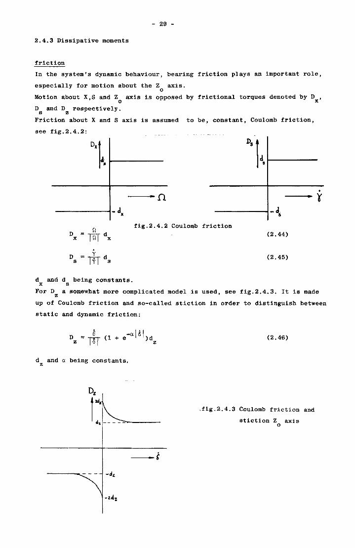
2.4.3 Dissipative moments
friction
In the system's dynamic behaviour, bearing friction plays an important role,
especially for motion about the Z axis. o
Motion about X,S and Z axis is opposed by frictional torques denoted by D , o x
D and D respectively. s z
Friction about X and S axis is assumed to be, constant, Coulomb friction,
see fig.2.4.2:
1), t I cl, 1------
• -----n -_. ¥ -----.... -d. It ------I-cJ a
n fig.2.4.2 Coulomb friction
d x
D d x =w x
. D = Y d
s ill s
and d being constants. s
(2.44)
(2.45)
For D z
a someWhat more complicated model is used, see fig.2.4.3. It is made
up of Coulomb friction and so-called stiction in order to distinguish between
static and dynamic friction:
8 -a\51 D = TTT (1 + e )d
z IVI z
d and a being constants. z
Dz
r eI .... - - - -"':::------
. ,
(2.46)
.fig.2.4.3 Coulomb friction and
stiction Z axis o
- 30 -
As for D • three effects have been neglected: z
- F • T and M • all three acting on the rotor, can not influence rotor z y behaviour directly (see par.2.3.2). They do however affect D • their z • contribution being a function of V, 0 and A.
- When both 6 and n are non-zero, the system behaves as a gyroscope.
The gyroscopical moment involved has an approximate magnitude of I no x
in which I represents the rotor's moment of inertia about the X axis. x • It may affect D • its effect being such that high 0 are opposed! z - The static loadings on the shaft's bearings and so D , depend on the z
vane's position relative to the shaft
the load
Under normal conditions, the rotor is coupled to a load, exerting a torque
QI on the rotor axis.
In general, this load torque is a function of the rotor's angular speed n and some load parameter S ( a field current for instance):
(2.47)
As for the load, any possible frictional torque will be assumed to be in
cluded in Ql or will be neglected.
- 31 -
2.5 The differential equations
2.5.1. Introduction
In this section the differential equations that constitute the model will be
derived.
First some introductory remarks on the differential equations will be made
(par.2.5.2).
Then in par.2.5.3 the differential equation for rotor motion about the X
axis is set up.
The differential equations for rotor motion about the S andZ axis are more o
difficult to derive. This is due to the fact that motion about S and Z axis o
can not be viewed apart from each other, since they are coupled mechanically.
In section 2.3 aerodynamic forces and moments on rotor and vanes have been
discussed. Obviously a number of them will appear in the equations governing
motion about S and Z axis. o
Yet we will first deal with mechanics only. i.e. with the question how motion
about S and Zo axis are coupled, disregarding for the moment the precise form
of the aerodynamic forces and moments involved (par.2.5.4).
This will be done by means of a mechanical analog of the system, using Lagran
ge's equations.
An alternative approach is made in APPENDIX I, using common Newtonian dynamics,
the results of which are valid for the ecliptic control system only.
Finally, returning to the original system, the differential equations gover
ning motion about S and Z axis will be set up. o
2.5.2 Introductory remarks on the differential equations
As stated earlier, the system is one with three rotational degrees of freedom.
The three coupled differential equations that govern its behaviour are, in
essence, torque. equations of the form:
moment of inertia x angular acceleration - Etorques = 0
Starting from this form, the differential equations for all three axes are
now viewed in more detail.
1. The torques involved in rotor motion about the X axis are:
Qr rotor torque eq.(2.18)
Ql load torque (2.47)
- 32 -
D moment of friction about X axis (2.44) x
The differential equation will take the form (par.2.5.3):
in which: I moment of inertia of rotor about X axis x
Q rotor's angular acceleration about X axis
2. For main vane motion about the S axis we already have:
(2.48)
M (F ) moment of aerodynamic force F (2.38) on main vane s mv mv
M (G) s
about Saxis
moment of gravitational force G on main vane (par.2.4.2)
on main vane about Saxis
Ds f.rictional torque about Saxis (2.45).
The differential equation will turn out to take the form:
I~y - M (F ) + M (G) + D ~ s mv s s
R = 0 s
(2.49)
in which: I moment of inertia of main vane about Saxis s ..
y angular acceleration of main vane about Saxis
R additional torque due to mutual interaction of shaft and s
main vane motion
3, For shaft and main vane motion about the Z axis we already have: o
M yawing moment (2.19)
M aerodynamic moment exerted on the shaft by the auxiliary av vane
M (F ) moment of aerodynamic force F (2.38) on main vane about z mv mv
Z axis o
D frictional torque about Z axis (2.46) Z 0
The differential equation governing motion about the Z axis will take the o
form:
I "
I 0 - M - M + M (F ) + D z av z mv z R = 0 z
(2.50)
- 33-
in which: I' moment of inertia about Z axis of the system as a whole. Z 0
..
It has an accent with it to indicate that it is not a
constant, but depending on the main vane's position and
motion relative to the shaft
o angular acceleration of shaft about Z axis o
R additional torque, due to mutual interaction of motion about Z
Sand Z axis o
Using Lagrange's equations, R and R as well as I' will appear to be found s Z Z
relatively easily.
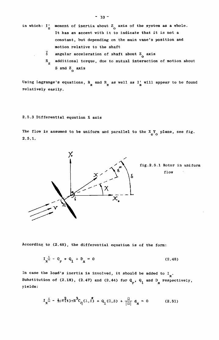
2.5.3 Differential equation X axis
The flow is assumed to be uniform and parallel to the X Y plane, see fig. o 0
2.5.1.
,/
fig.2.5.l Rotor in uniform
flow
According to (2.48), the differential equation is of the form:
I Q - Q + Q + D = 0 x r 1 x (2.48)
In case the load's inertia is involved, it should be added to I . x
Substitution of (2.18), (2.47) and (2.44) for Qr
, Ql
and Dx respectively,
yields:
(2.51)
- 34 -
the differential equation for rotor motion about the X axis, in which
• d 0 -X(t) see fig.2.5.1 (2.2)
), == ~ (2.9) V(t)
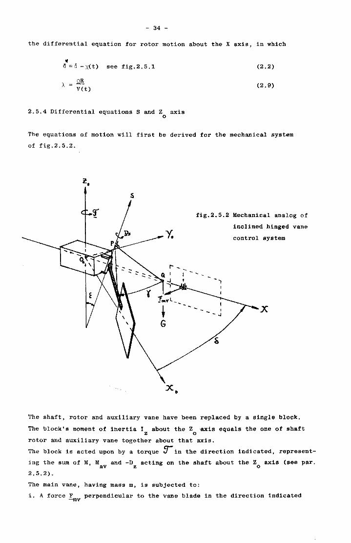
2.5.4 Differential equations Sand Z axis o
The equations of motion will first be derived for the mechanical system
of fig.2.5.2.
s
fig.2.5.2 Mechanical analog of
inclined hinged vane
control system
x
The shaft, rotor and auxiliary vane have been replaced by a single block.
The block's moment of inertia I about the Z -axis equals the one of shaft Z 0
rotor and auxiliary vane together about that axis.
The block is acted upon by a torque sr-in the direction indicated, represent
ing the sum of M, M and -D acting on the shaft about the Z axis (see par. av Z 0
2.5, 2).
The main vane, having mass m, is subjected to:
i. A force F perpendicular to the vane blade in the direction indicated -mv
- 35 -
ii. The force of gravity ~, acting downwards (for cQnvenience, !mv and G
are only shown for the dQtted vane, i.e. the vane in its lowest posi
tion)
iii. A torque D due to friction about the Saxis s
The coordinate systems to be used equal those of p~r.2.2.3.
As can be easily verified, this mechanical system h~s two degrees of free
dom: Two independent coordinates are required to specify completely the
position of both its component parts.
Here we will use 0 and y (fig.2.5.2 and par.2.2.3), specifying the position
of the block and the vane respectively.
The equations of motion will be obtained by applying Lagrange's equations.
For this mechanical system they are:
= Fl( (2.52a)
(2.52b)
y and 0 are referred to as generalized coordinates.
T, representing the system's total kinetic energy, should be expressed in
terms of these generalized coordinates and their derivatives.
The so-called generalized forces Fy and Fo' that appear at the right-hand
sides of (2.52) can be found by writing out an expression for the work ~W y
and ~Wo ' done by all applied forces and moments on the block and the vane,
which must shift in position as a result of an infinitesimal increase ~y in
y and ~o in 0 respectively. Then from the relations:
(2.53a)
(2.53b)
Fy and Fo follow at once.
When there are conservative forces among the forces applied, so that they can
be derived from some potential function V (F=-gradV), (2.52) may be written
as:
(2.54a)
(2.S4b)
- 36 -
in which L, the Lagrangian function, is defined as:
L:: T-V (2.55)
In (2.54) it is assumed that V in not a function of i and ,.
L too, should be expressed in term of the generalized coordinates ¥ and &. The generalized forces are found in the way indicated above, but now taking
account of the non-conservative ones only.
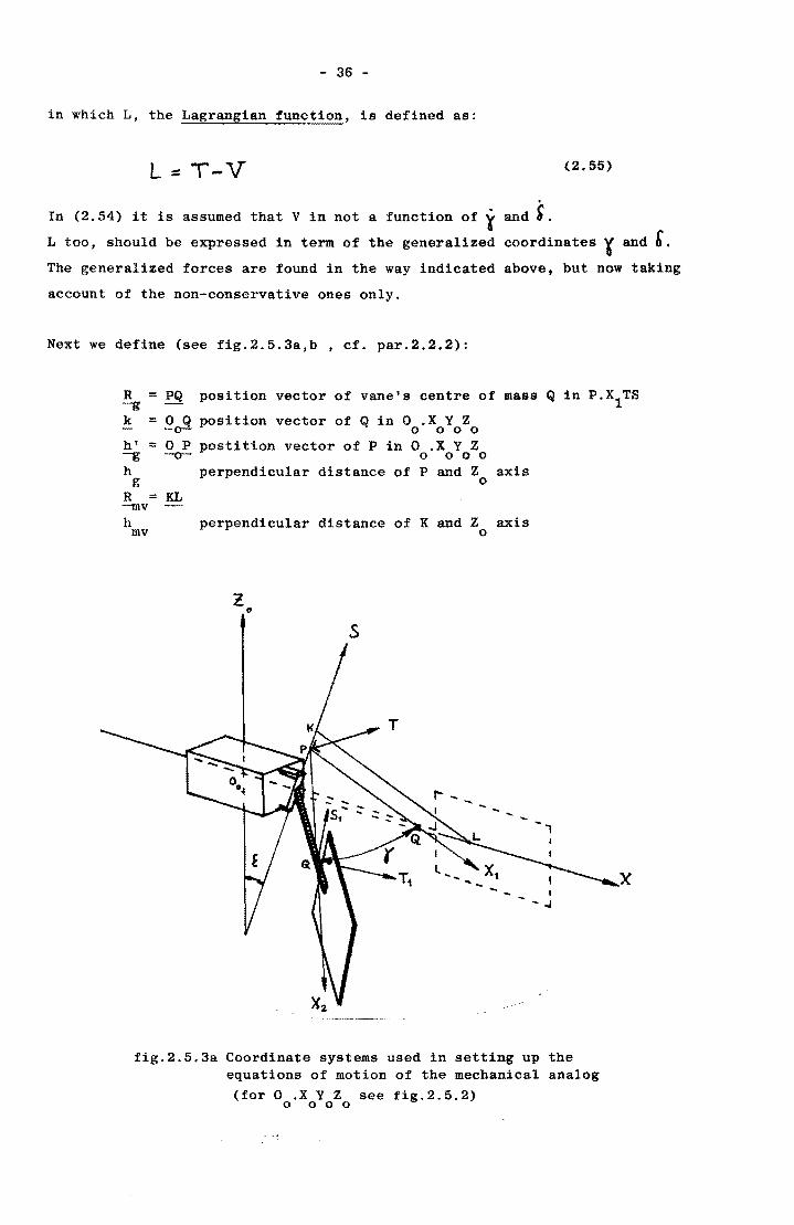
Next we define (see fig.2.5.3a,b , cf. par.2.2.2):
R = PQ -g
position vector of vane's centre of mass Q in P.X1TS
k = ht = -g h
g
o Q position vector of Q in 0 .X Y Z -0--- 0 0 0 0
o P postition vector of P in 0 .X Y Z -0-- 0000
perpendicular distance of P and Z o
R = KL -mv
axis
h perpendicular distance of K and Z axis mv 0
2 o
s
fig.2.5.3a Coordinate systems used in setting up the equations of motion of the mechanical analog (for 0 .X Y Z see fig.2.5.2)
o 000
- 37 -
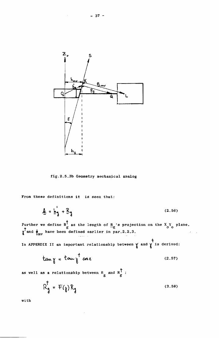
s
L
h
fig.2.5.3b Geometry mechan.ical analog
From these definitions it is seen that:
Further we define Rt as the length of R 's projection on the X Y plane. g -g 0 0
ltand tmv have been defined earlier in par.2.2.3.
t In APPENDIX II an important relationship between ~ and ~ is derived:
as well as a relationship between R g
with
and Rt g
(2.57)
(2.58)
- 38 -1
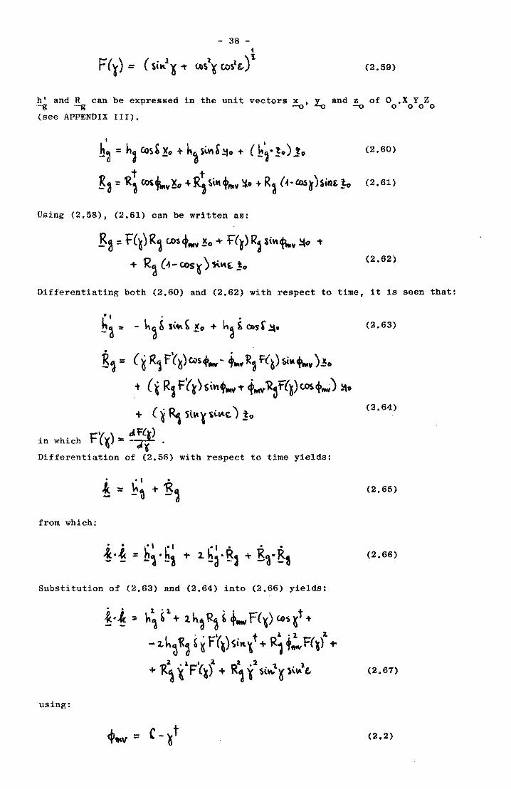
F (¥) = ($'tt~ -t (,O~l~ cost£...) 1
(2.59)
hI and R can be expressed in the unit vectors x , y and z of 0 .X Y Z -g -g ~ "'-0 ~ 0000
(see APPENDIX III).
. , hd = h, (45~~o + h~S~~'!10 + (~f!o)jo
Ea = 'R~ co~tIrlV!o +R; ~i"'t"'V ~o + Ra (.t- C05 K)Slnt!-o
Using (2.58), (2.61) can be written as:
Ea = F(~) 1<1 c.os+ftIV!o -+ +(~) R, SiVl<l\n ~o -t
+ 1(~ (" ... <:.os ~ ) 1\.Vl£ !o
(2.60)
(2.61)
(2.62)
Differentiating both (2.60) and (2.62) with respect to time, it is seen that:
. , . h~:It - h~ ~ '"" ~ ~o + h~ £ OISr.~. . , . IS,:: (i R, F(~)~s+_ - +lftt 'R, F(~) ~lM'-" ).30
t (~R1f~~)$\~+..,'t ~MV'R3f(l)c.os.+lIW) 110
+ (~~ Sl\t"i~(' ) ,!o
r'f. ) = ~\l~ inWhichrl~ tAl" Differentiation of (2.56) with respect to time yields:
from which:
Substitution of (2.63) and (2.64) into (2.66) yields:
!.!:: h,'2.+ lh~'R~'+_f('()cos~t+ - :z.h~ 1<4' i F'(\)~irt~t + R; +~F(¥)2. i-
l. .a. I 1 I ,1 1. 1 ... 'R~ ~ Flk) + R,,, Silt\, ~ )i~ l,
using:
(2.63)
(2.64)
(2.65)
(2.66)
(2.67)
(2.2)
- 39 -
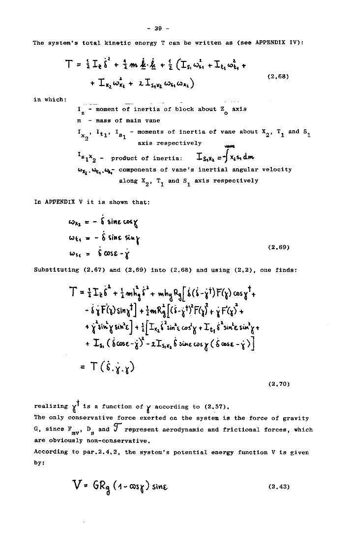
The system's total kinetic energy T can be written as (see APPENDIX IV):
(2.68)
in which:
I - moment of inertia of block about Z axis z 0
m - mass of main vane
I ,Itl , ISl - moments of inertia of vane about X2 , Tl and S1 x2 axis respectively WMe
product of inertia: I s"x1 =-/ x,~ c:l."" ~.l'~t.~t components of vane's inertial angular velocity
along X2 , T1 and S1 axis respectively
In APPENDIX V it is shown that:
. "'11.1 :: - , 'flint c..os. '(
W~i ,. - ~ ~i .. t $i"'t wst 1\11: G cost - ~
(2.69)
substituting (2.67) and (2.69) into (2.68) and using (2.2), one finds:
T :llI~,1 T llM .. ;rl -to ~ha~[i(~-it)F(I)c.oSlt+ - & i F(")~in~t] + IftI~;[(S-~ttf(~t t ~ t(¥):l +
+ ~ \ii ~ ,, .. I t ] i i [ IJ(l '\ml.t Go$l~ + Itt f' 5i..le:. 'iul~ +
+ Is. (~W$t -i)t. - %.ISIX1 t ~i.hL CNS ~ (S COi& -" )]
realizing ~t is a function of r according to (2,.57).
(2.70)
The only conservative force exerted on the system is the force of gravity
G, since F t D and ~ represent aerodynamic and frictional forces, which mv s are obviously non-conservative.
According to par.2.4.2, the system's potential energy function V is given
by:
(2.43)
- 40 -
The Lagrangian function L (2.55) is then found by subtracting (2.43) from
(2.70).
Carrying out the differential operations on L in a straightforward manner
according to (2.54), would yield an enormous amount of terms, containing,
in addition to b, l' ~tand their derivatives, F(¥) and its derivatives with
respect to I' It is therefore that an approximation is made at this point.
The Lagrangian function will be expanded in a MacLaurin series of the form:
(2.71)
l Neglecting terms of order ~ and higher, the differential operations of (2.54)
will be carried out.
For F(~) one finds:
From (2.72):
For It, from (2,57):
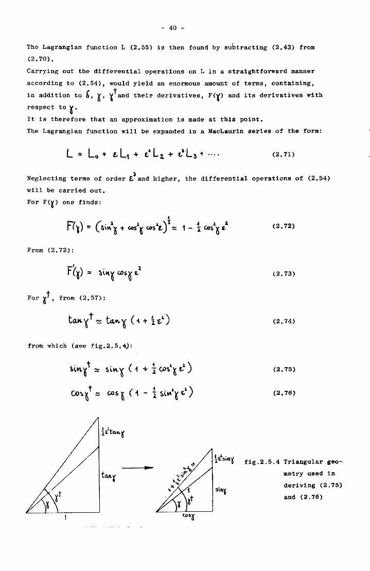
from which (see fig.2,5.4):
f.~~ l t ::t S \.11\.'( (.1
(x)\~t = GOS~ (1
....
(2.72)
(2.73)
(2.74)
(2.75)
(2.76)
fig.2.5.4 Triangular geo
metry used in
deriving (2.75)
and (2.76)
- 41 -
Defining:
(2.77)
rl t . (.l ) n,\I\. ~ ~ 'S'\.\I\. ~ -t + l <:.os t.t t,t
= h"'-(~-t(l). ~'( + (3 eosCf (2.78)
from which
(2.79)
and
(2.80)
o For &=15 , approximations (2.72) and (2.79) are both better than .1%.
substituting (2.72), (2.73), (2.75), (2.76), (2.79) and (2.80) into (2.70),
one finds, neglecting terms of order &3 and higher:
for the terms containing mh R : g g
~\.t~ ~ r t(,_~1) f(~)Q)Sxt - t ~ fr~)$(~,t]
~ M ~1 ~ [ ~ (' -j ) - t ~t (.OS ~ ,1J
Equation (2.43) for V becomes:
Collecting terms, one finds for Lo' L1 pnd L2 respectively:
(2.81)
(2.82)
(2.83)
(2.84)
- 42 -
(2.85)
For the main vane's moment of inertia I about the S axis, one can write: s
(see fig.2.5.3.a)
(2.88)
Using (2.88), (2.85) and (2.87) may be written as:
(2.89)
(2.90)
Since the differential operators in (2.54) are linear, Lo' Ll and L2 may
be treated separately:
- 43 -
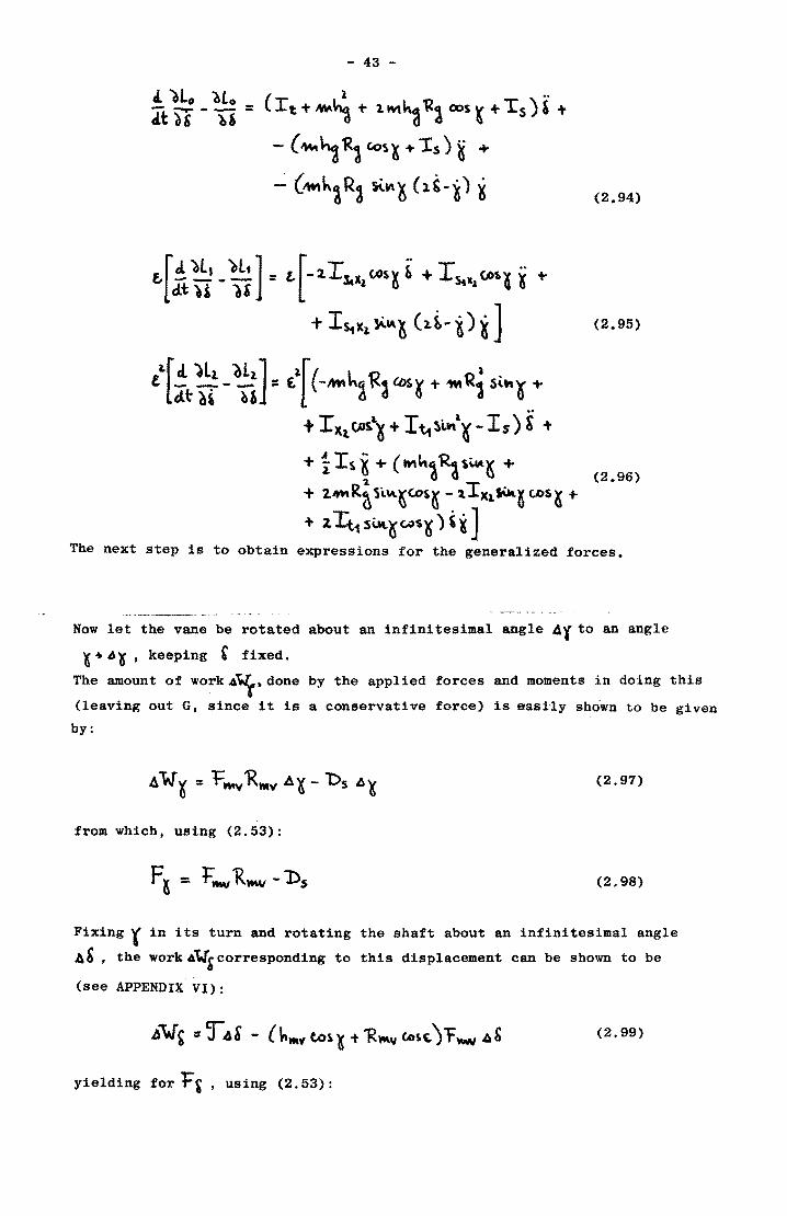
! ~ -~ = (It T ~h~ ... 1. tv1k4 'Ret cos v + Is) & ... tLt ), 0' '0 a <l \\
- (~~ 'R~ Cos ~ + 1:s ) ~ +
~ (!WI ~~ R~ $i.", ~ (1' -~) ~
t..[~ ~ -~] =- t.[-2.I14Xl to5X r; + I s•l ! to'l j ... dt ~1 dS
+ I~x1. "'~~ Cl.t- ~) ~ ]
£'[it ~-~] = El[(_ .... ~ R3 ""~ + ... ~ $'''~ +
+ Ixl. (.OS~~ + It. ~i.\,\l~ - Is ) ~ +
+ i Is ~ + ( .... t...d ~ $i.4.t~ +
+ 2.~R~ 'Si.\I\.~(.os~ -1IX1$iJ.t~ (..OS~ ...
+ 2. Tt1 S""~CN'i~ ) ,~ ]
(2.94)
(2.95)
(2.96)
The next step is to obtain expressions for the generalized forces.
Now let the vane be rotated about an infinitesimal angle 41 to an angle
l +.6l ' keeping , fixed.
The amount of work4~.done by the applied forces and moments in doing this
(leaving out G, since it is a conservative force) is easily shown to be given
by:
(2.97)
from which, using (2.53):
(2.98)
Fixing r in its turn and rotating the shaft about an infinitesimal angle
AS , the work 4V, corresponding to this displacement can be shown to be
(see APPENDIX VI):
(2.99)
yielding for F~ , using (2.53):
- 44 -
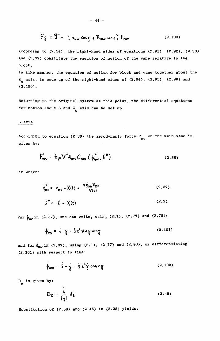
(2.100)
According to (2.54), the right-hand sides of equations (2.91), (2.92), (2.93)
and (2.97) constitute the equation of motion of the vane relative to the
block.
In like manner, the equation of motion for block and vane together about the
Zo axis, is made up of the right-hand sides of (2.94), (2.95), (2.96) and
(2.100).
Returning to the original system at this point, the differential equations
for motion about Sand Z axis can be set up. o
Saxis
According to equation (2.38) the aerodynamic force F on the main vane is mV
given by:
(2.38)
in which:
(2.37)
(2.2)
For +M~in (2.37), one can write, using (2.1), (2.77) and (2.79):
(2.101)
And for +Mvin (2.37), using (2.1), (2.77) and (2.80), or differentiating
(2.101) with respect to time:
D is given by: s
Ds
Substitution of (2.38) and (2.45) in (2.98) yields:
(2.102)
(2.45)
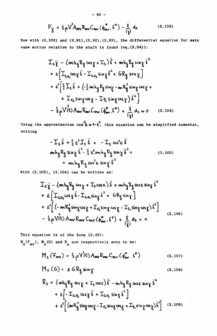
- 45 -
(2.103)
Now with (2.103) and (2.91),(2.92),(2.93), the differential equation for main
vane motion relative to the shaft is found (eq.(2.54»:
Is~ - (..m~,'R, c.os~ + Is)' -+ *,h~~ Si~~ ,1-T £ [IS,x
1CoS lr ~ - I SIl(l \~"'~ &1 + GR1 s-;.~ ~ ]
1.[" I" ( 1 + E.. I s~ + -i'*~aR3S\~~-*,~~$i"~c.oS1(+
+ I)(~ s"" ~ ~ ~ - I 't\ ~ ~ ~ OI~ '( ) ~ ~ ] :1 •
- ~fV(t)A ... v'RMVCVMV (,:.~IE) + ! lAs:= 0 . I"~ (2.104)
2 I. Using the approximation cos &~4-t, this equation can be simplified somewhat,
wri ting
.. ~.. .. - Is! + 1 £, Is & = - Is Cos'£.'
·1 '\ l, 'R '1
~h~ 'R~ ~IA ~ , - 'i £. ~"'a ~ SiM~ b = (2.105)
'1 • 1
=- iW\,h~ 'R~ Co~ £,. S\.~'( S
With (2.105), (2.104) can be written as:
(2.106)
This equation is of the form (2.49):
M (F ), M (G) and R are respectively seen to be: s mv s s
M s (Fmv) = 1 (' Vl(t).A tKV ~'"" c..,v (ct: . &*) (2.107)
M,CG):: l.6R~<i\."'¥ (2.108)
'Rs = (M~ ~ o.,~ ~ i- TS c.ou:) ( - "'" h~ R, (0,£ si"'l ~ a-
t f.[- I sIxz ())S~, + IStltl, S\~l t1] T £t[ (""~i Si"lCO'~- IlCl ~~~(p'~ +It,Sh'~""~) ~1] (2.109)
- 46 -
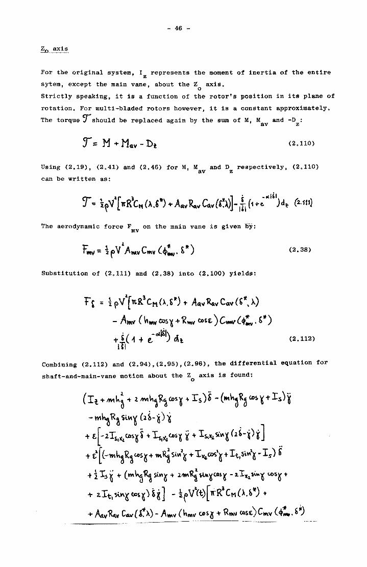
axis
For the original system, I represents the moment of inertia of the entire z
sytem, except the main vane, about the Z axis. o
Strictly speaking, it is a function of the rotor's position in its plane of
rotation. For multi-bladed rotors however, it is a constant approximately.
The torque ~shoUld be replaced again by the sum of M, M and -D : av z
(2.110)
Using (2.19), (2.41) and (2.46) for M, M and D respectively, (2.110) av z
can be written as:
The aerodynamic force F on the main vane is given oy: mv
Substitution of (2.111) and (2.38) into (2.100) yields:
t~ ::: tf>VlltRlC..tt(A.&t) T A""'Ro.,,CtW('~) .. )
- Afft'l (~ww C>s ~ -+ ~*" to~€. ) C.w.r (ct:V . ~")
l' ~( ~ + e.-allil) mt hi
(2.38)
(2.112)
Combining (2.112) and (2.94),(2.95),(2.96), the differential equation for
shaft-and-main-vane motion about the Z axis is found: o
(Ii. + IM~~ + 2. IWlh1 ~~ Gosl "" Is)S - ( .... hO ~d Go!, ~ l' Is) i - Wl~ 'R~ ~il'l~ (li- ~) ~
+E.[-lI; ... "",i. I~>(o ..... ~ ¥ + Is. .. 5i.~ C.'-l)i] + ([(-'WIh~ R~ (.os~+ 'tI\~ SiV\2G + TXJCO'1.\~ + ItISiVl) - Is) ~
+iI.5~ + (m~~s\W\~ 1- l~~\t-Kw~ -2.Ixt.'"''6' U>S~ ..
+ 2.It\5t\,\~(jgs~)~~] - I~Vl.(t)[1rR)CM(A.b*) +
... A..v'&tv c .. ,,( !~).) - A",,, (h",y ~S~ -+ RnI." ~s£)C",v (,:.. b')
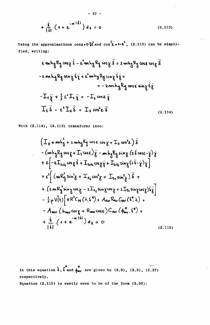
- 47 -
, _ ... 16)
+ ITt (-i + e. ) J.} = 0 (2.113)
t' 2 1 Using the approximations cost'1-~t and cos l,a"-E. , (2.113) can be simpli-
fied, writing:
". a.... ... a.~hO R~ CDS~ ~ - €.'W\~?, ~1 c..os~ S : l'm~O ~~ ~f CD~~ ~
-2.1M~1~ ~~l 'i + f.lNll\"'a~ \iM~ ~~ ': = - '2.lW\h~ ~1 CO~E $~~ ~~
-Is~ + i t1Is i = -Is CO$&~'
I S ~ - t. 1 Is ~ = I S cosl. £, S
With (2.114), (2.113) transforms into:
(I~+"""~i + ~~~R~ LOS£. (.i)fI~T I~ CO$lt,) ~
- (.~",h~R~ GOs{+Isc.ost)~ -..m~~R3S~~~ (1'CASE-~)i
t t [ -~IStlCz. UX ~ , + 15111 (;)S X ~ + ISllt1 S~"~ (2. ~ -~ ) ~ ] 1.[ ( 2 1 ••
... £ ~~ S~\A. ~ + Ixz cosl
O -to It1 S~~ ~ b +
+ (2"" R{ .. " ~ <0< ~ - IT., ....... 1\"" ~ uIt, ,u.~,". t)t ~ ] - f e V(i:) [ trR1CH (~. ~ tt) + AQAr'Rctv C4 " (~~.\) +
- A""" (h",,, Cos 1 + RM\I (A:)S& ) C tIlV (,.! . ,~) +
6 -ed")
(2.114)
+ -:- (-1 + e. tA'i' = 0 1" (2.115)
.. * In this equation A, , and + ... ~ are given by (2.9), (2.2), (2.37)
respectively.
Equation (2.115) is easily seen to be of the form (2.50):
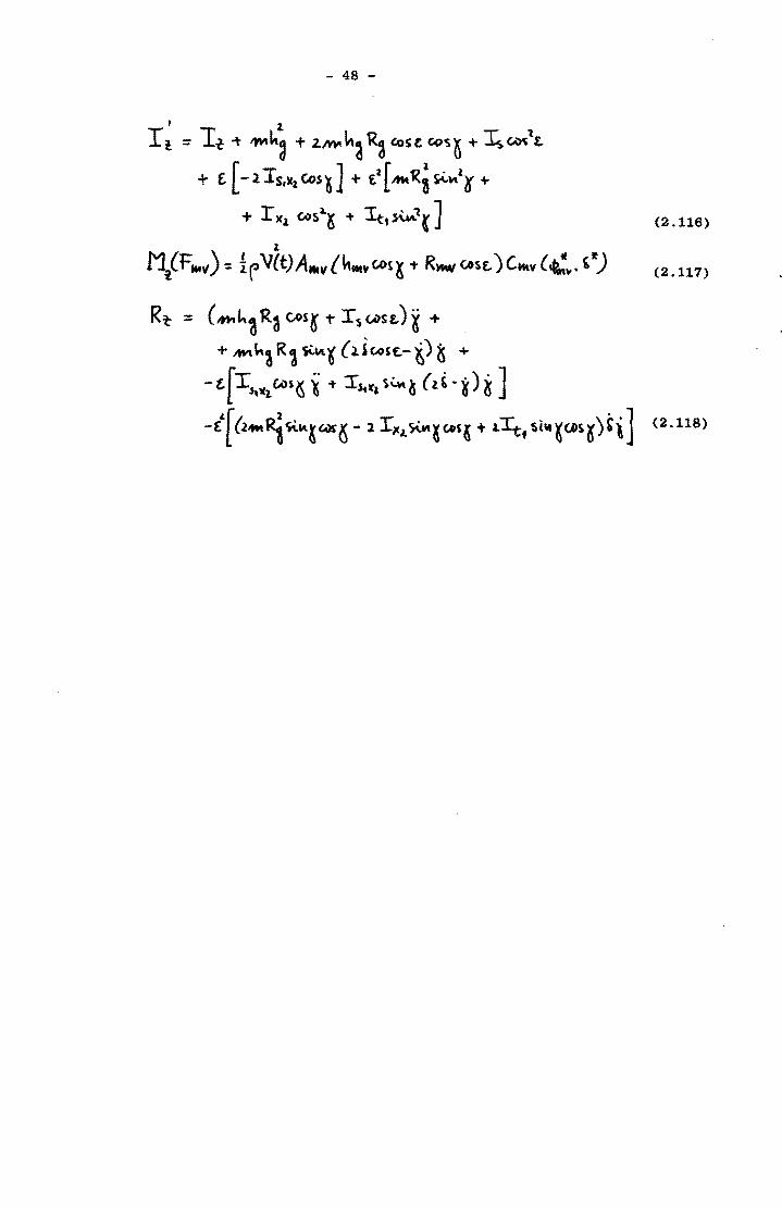
- 48 -
, 1.
Ie::; Ii- l' ~ k3 + 2.~ ka ~ GoS t: GO'S n ... I:. GoiX It.
+ £ [-2 Is,,! CoS~] + f.l[ A'tl~3 ~"",l.~ +
... r It.l CAlS~~ -+ It1 ~t ] 1
MiF ... ~): fl"V(t)A ... v{\, .... c.o\:~ ... R*YC'Ost.)C .... ,,("'~. ,~)
Rt = (Nhh~ Ra c;.os~ TIs (;oS&) ~ +
T hll\h~ R1 ~~ (;tiCAlSt:.-~) ~ +
-t[ IS'''l c.os~ i -+ I SIIC, s':''''~ (l~ - ~) ~ ]
(2.116)
(2.117)
-l[ 6It1tRi~tl~G!)f~ - 1 I,l(l.Si.""lCRS~ + 1.Itf $i"~C»S~)'\] (2.118)
- 49 -
2.6 Preset angles
2.6.1 Introduction
In general both the main vane and the auxiliary vane possess so-called
preset angles in order to improve the system's behaviour.
In the following paragraphs it will be pointed out briefly what their effects
are on the sytem's control properties.
It will also be indicated what changes should be made in the system's diffe
rential equations when a preset angle for the main vane is employed.
2.6.2 Preset angle auxiliary vane
As stated in par.2.2.2 the auxiliary vane may have a preset angle ~ , which
is defined as the angle between the vane's blade and the rotor plane (YZ plane).
The auxiliary vane is often given a preset angle in order to improve the sys
tem's behaviour.
As for the system's dynamic behaviour, preset angles for the auxiliary vane
have been found to be of much interest as stabilizing devices.
Results of windtunnel tests concerning both static and dynamic behaviour for
several preset angles will be given in section 5.4.
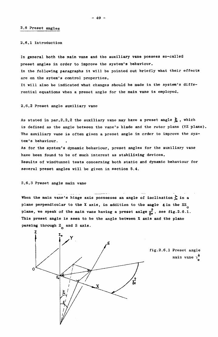
2.6.3 Preset angle main vane
When the main vane's hinge axis possesses an angle of inclination~ in a
plane perpendicular to the X axiS, in addition to the anile ~in the XZ o
plane, we speak of the main vane having a preset anlge~!, see fig.2.6.1.
This preset angle is seen to be the angle between X axis and the plane
paSSing through Z and Saxis. o
z
fig.2.6.1 Preset angle
main vane yt o
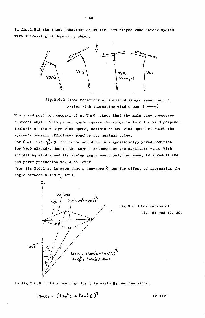
- 50 -
In fig.2.6.2 the ideal behaviour of an inclined hinged vane safety system
with increasing windspeed is shown.
t V
V'llfO
fig.2.6.2 Ideal behaviour of inclined hinged vane control
system wi th increasing wind speed (-)
The yawed position (negative) at V = 0 shows that the main vane possesses
a preset angle. This preset angle causes the rotor to face the wind perpend
icularly at the design wind speed, defined as the wind speed at which the
system's overall efficiency reaches its maximum value.
For ~:&o, 1.e, ... ! .. o, the rotor would be in a (positively) yawed pOSition
for V = 0 already, due to the t.orque produced by the auxiliary vane. With
increasing wind speed its yawing angle would only increase. As a result the
net power production would be lower.
From fig.2.6.1 it is seen that a non-zero ~ has the effect of increasing the
angle between Sand Z axis, o
S fig.2.6.3 Derivation of
(2.119) and (2.120)
In fig.2.6.3 it is shown that for this angle ~ one can write:
1
tQM.t1 :. (ttL"'1. £ + t~l. t. )1 (2.119)
- 51 -
and, for t! : t tdM.t,
~'10· -.. t~t (2.120)
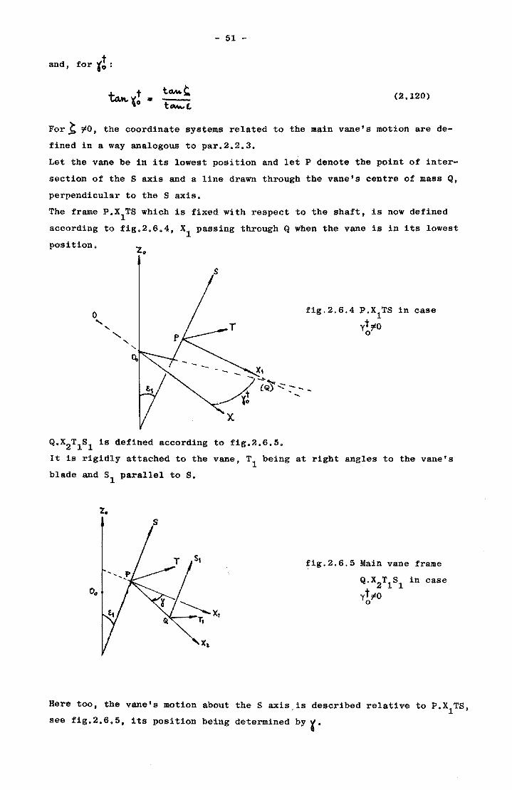
For ~ ~O, the coordinate systems related to the main vane's motion are de
fined in a way analogous to par.2.2.3.
Let the vane be in its lowest position and let P denote the point of inter
section of the 8 axis and a line drawn through the vane's centre of mass Q,
perpendicular to the 8 axis.
The frame P.X1TS which is fixed with respect to the shaft, is now defined
according to fig.2.6.4, Xl passing through Q when the vane is in its lowest
pOSition.
o " " "
s
" "
Q.X2T1S1 is defined according to fig.2.6.5.
fig.2.6.4 P,X1
TS in case
yt~o o
It is rigidly attached to the vane, T1 being at right angles to the vane's
blade and 81
parallel to S.
~ig.2.6.5 Main vane frame
Q.X2
T1
S1
in case
yt~o o
Here too, the vane's motion about the S axis,is described relative to P.X1
TS,
see fig.2.6.5, its position being determined by l'
- 52 -
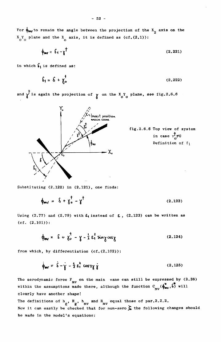
For ,mvto remain the angle between the projection of the X2
axis on the
X Y plane and the X axis, it is defined as (cf.(2.1»: 000
(2.221)
in which '1 is defined as:
(2.222)
and l is again the projection of r on the XoYo plane, see fig.2.6.6
~------------~-------Xo
Substituting (2.122) in (2.121), one finds:
f1g.2.6.6 Top view of system
in case yt;tO o
Defin1 tion of 01
(2.123)
Using (2.77) and (2.79) with t. instead of t., (2.123) can be written as
(cf. (2.101»:
(2.124)
from which, by differentiation (cf.(2.102»:
(2.125)
The aerodynamic force F on the main vane can still be expressed by (2.38) mv * r*
within the assumptions made there, although the function C (~MV'O) will mv T clearly have another shape!
The definitions of h , R , h and R equal those of par.2.2.2. g g mv mv
Now it can easily be checked that for non-zeroJ; the following changes should
be made in the model's equations:
- 53 -
i.. £ should be replaced by £1 everywhere (eq. (2.119»
.d. instead of (2.101) and (2.102), (2.124) and (2.125) should be used respect
i vely, ¥t being given by (2.120)
- 54 -
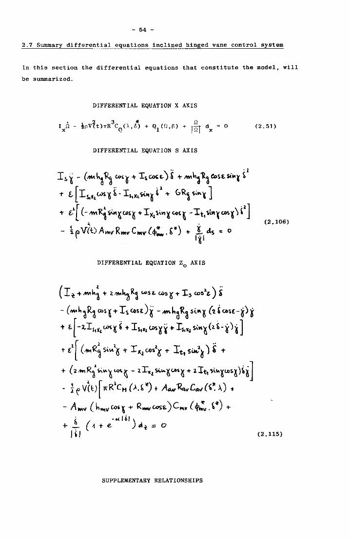
2.7 Summary differential equations inclined hinged vane control system
In this section the differential equations that constitute the model, will
be summarized.
DIFFERENTIAL EQUATION X AXIS
DIFFERENTIAL EQUATION SAXIS
-, . 1
I s ~ - (MIt h~ 1 Got; ~ -+ Is. ~ £-) & -t-,om ka 'R~ &s [. Si" ¥ ~
... e. [ I SIll eNS l ~ - IslXa. ~t\~ C -+ &R1 '5~t\ '( ]
T £,l[ (-IM'R'sitot~c.oSK +I)Cl\illl~Cot' -It\\tM~c.osl),lJ 1 •
- t(.)V(t)Anti'Rn."CMV(+!...'W) + ! as:: 0 \ .... Iii
DIFFERENTIAL EQUATION Zo AXIS
(I ~ + M'lki + 2.!WI~ ~ ('os £. (4):) ~ T I'., ('()51~ ) ~
- (~hdRd (;Os, T Is C6U:)~ - ..... h~f{3 s~.~ (2' O>Sf-~) ~
+ L [ -l.ISilCL <..eX ~ , + I S• X1 (;IS X ~ + rilll. Si.~ (2.' -~ ) ~]
T l[ (""R~ S,,,,l~ + I •• CAls1K .. It, s~~ ) ~ T
+ ('''''R{ " .. ~ -~ - lI •• -~"'.~ +11t. ·U.l ... ·~ )~l] - ! e vet:) [ «R1CH (A.' *) t AAu ~CCl" ('~).) ...
- AM" (h!l¥l\l Cos l -+- R"",GoS&) CtI\y (,.:, • ~~) +
f, -edi,)
(2.51)
(2.106)
+ _, (-t + e fA!, = 0
'" (2.115)
SUPPLEMENTARY RELATIONSHIPS
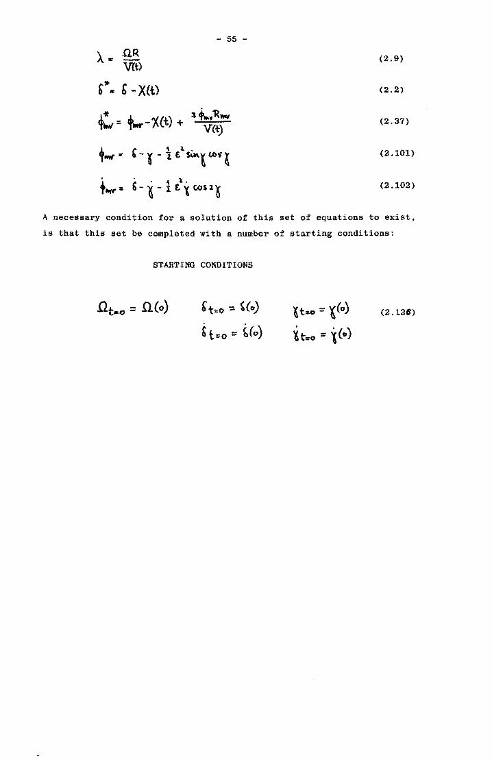
- 55 -
A- nR (2.9) -Vet)
,,.. b - X{t) (2.2)
~ 3 + ... "R_ +"'" = t--'X(t) + V(.f;) (2.37)
''''' or
, "t . -, - 1. t Sl.M.l u>s ~ (2.101)
. , - ~ - 1 £t ~ CO$ 1 ~ ;11'1'1': (2.102)
A necessary condition for a solution of this set of equations to exist,
is that this set be completed with a number of starting conditions:
STARTING CONDITIONS
bt=O :; ~(o)
t teo ::: teo) l t=o ::: ,(0)
'(teo = l(o)
(2.126)
- 56 -
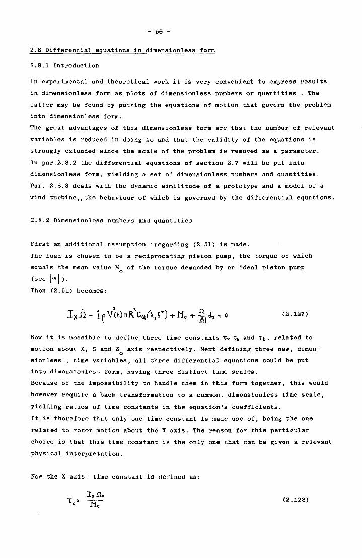
2.8 Differential equations in dimensionless form
2.8.1 Introduction
In experimental and theoretical work it is very convenient to express results
in dimensionless form as plots of dimensionless numbers or quantities. The
latter may be found by putting the equations of motion that govern the problem
into dimensionless form.
The great advantages of this dimensionless form are that the number of relevant
variables is reduced in doing so and that the validity of the equations is
strongly extended since the scale of the problem is removed as a parameter.
In par.2.8.2 the differential equations of section 2.7 will be put into
dimensionless form, yielding a set of dimensionless numbers and quantities.
Par. 2.8.3 deals with the dynamic similitude of a prototype and a model of a
wind turbine" the behaviour of which is governed by the differential equations.
2.8.2 Dimensionless numbers and quantities
First an additional assumption regarding (2.51) is made.
The load is chosen to be a reciprocating piston pump, the torque of which
equals the mean value M of the torque demanded by an ideal piston pump o
(see 14"1 ) . Then (2.51) becomes:
(2.127)
Now it is possible to define three time constants ~V,T6 and Tt, related to
motion about X, Sand Z axis respectively. Next defining three new, dimen-o
sionless , time variables, all three differential equations could be put
into dimensionless form, having three distinct time scales.
Because of the impossibility to handle them in this form together, this would
however require a back transformation to a common, dimensionless time scale,
yielding ratios of time constants in the equation's coefficients.
It is therefore that only one time constant is made use of. being the one
related to rotor motion about the X axis. The reason for this particular
choice is that this time constant is the only one that can be given a relevant
physical interpretation.
Now the X axis' time constant is defined as:
(2.128)
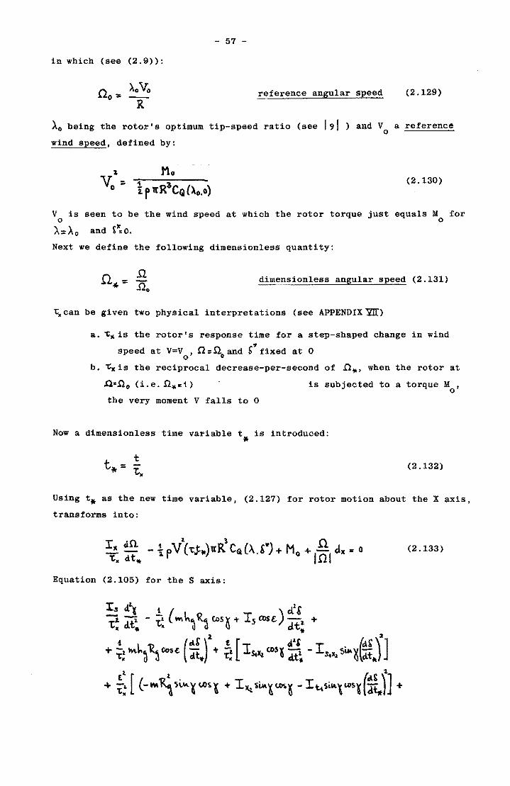
- 57 -
in which {see (2.9»:
reference angular speed (2.129)
AO being the rotor's optimum tip-speed ratio (see 191 ) and V a reference o wind speed, defined by:
~
V:::. o
Mo (2.130)
V is seen to be the wind speed at which the rotor torque just equals M for o 0
A=Ao and tlr: O.
Next we define the following dimensionless quantity:
dimensionless angular speed (2.131)
't. can be given two physical interpretations (see APPENDIX W)
a. -C" is the rotor's response time for a step-shaped change in wind 'II
speed at V=V , .Q::: nand b fixed at 0 o 0
b. ~is the reciprocal decrease-per-second of !)., when the rotor at
,a .. n o (Le . .0 .... 1) is subjected to a torque M , o
the very moment V falls to 0
Now a dimensionless time variable t. is introduced:
(2.132)
Using t. as the new time variable, (2.127) for rotor motion about the X axis,
transforms into:
(2.133)
Equation (2.105) for the Saxis:
1:" d,ll t ( ) d.2& "'-t!:it!. -:a W\h'a 1(~ c.>sn ... Is (x)s£. clt: +
+ ~ "'I.~ ~ ... c (~t.,f + ~ [ I"" " .. , ~ - I .... sUo ~~.lJ + ~~ [ (-"'R1 ~'-~~ ('()"'l + I~ $",~ ~~ .. I~StllL' lDsl(lll] ...
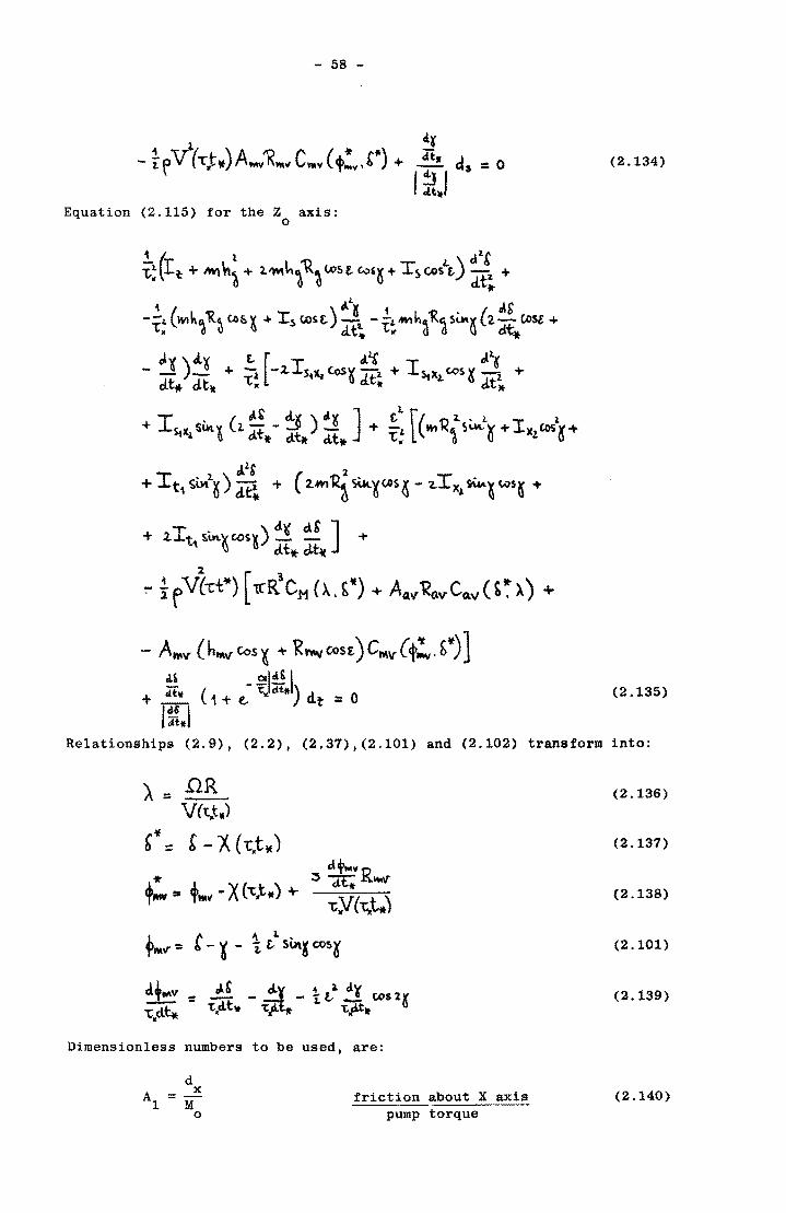
- 58 -
Equation (2.115) for the Z axis: o
1 f-r 1. ) ,,1& 'i"!\" i: + 1W\t.~ + 2.'W\~61<~(.oStCo'~+ Tsc.os't d.t1 +
~
i ( ) 6..1.5 1 ( J,g -i; WI h ~ 'R~ t;)~ ~ + rs (;os t :it~ - i; tM hd'Rd SlM ~ 2. D.~ (;}St +
J" )..A.~ L [T Ii~ I £ll.K - - - + 1 -.t St~ (.oSn 't}. + ~x~ cos ~ --'i +
cL~ <Lt. 1:,. a. 'It dtJt
I . (ilt d,l() d.~ ] £4 f( 1"12.. 1. I 1 + Stlt]. SI.tl ~ 2. tit. - ttit dt* + 't; l IN! "'~ S\.\I\., ~ + )(1. C05 K +
tAlG 1
+ It" sul~) d:tt. + (2.Wl1 Sik.~(A)S~ - ,Ix ... ~~ to$~ +
+ .tIt" SoiA'IGOsl) ~ tiS' ] + I,) clt. cLt-w
~ IrV(-rt*) [lCIfeM (A. ~*) + Atl"~ClVCo.V(~~ X) +
- A~v (h...,Cos~ + Rr't\yCOSt)CMV'(;~'S*)}
(2.134)
.4' _ ~I:! I + cUll ( 1 + (.. ~ it) dt ::: 0 (2.135)
I~*I Relationships (2.9), (2.2), (2.37),(2.101) and (2.102) transform into:
Dimensionless numbers to be used, are:
d A =~
1 M o
friction about X axis pump torque
(2.136)
(2.137)
(2.138)
(2.101)
(2.139)
(2.140)
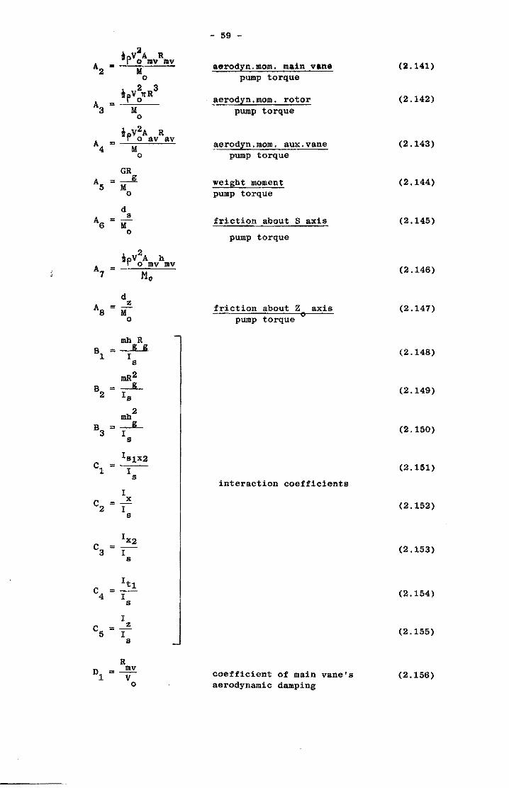
• V2
A R P 0 IIlV IIlV A • 2 M
o
trV!'ltR3
Aa = M o
i V2A R P 0 av av M
o
GR A =---K
5 M o
d s
A6 = M o
mbR
B1 = --f-K s
mR2
B2 = ~ Is
mb2
B3=~ s
- 59 -
aerodyn.mom. main vane pump torque
aerodyn.mom. rotor pump torque
aerodyn.mom. aux. vane pump torque
weight moment pump torque
friction about Saxis
pump torque
friction about Z axis o pump torque
interaction coefficients
coefficient of main vane's aerodynamic damping
(2.141)
(2.142)
(2.143)
(2.144)
(2.145)
(2.146)
(2.147)
(2.148)
(2.149)
(2.150)
(2.151)
(2.152)
(2.153)
(2.154)
(2.155)
(2.156)
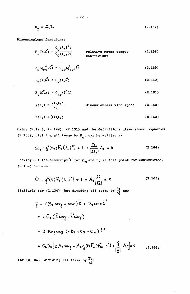
- 60 -
Dimensionless functions:
'It .. it 11-F2(~ .t> = c (+ .'> Tmv mv mv
F4(~~).) = C (S~).) av
g(t,.) = V(t,t,.) V
o
relative rotor torque coefficient
dimensionless wind speed
(2.157)
(2.158)
(2.159)
(2.160)
(2.161)
(2.162)
(2.163)
Using (2.128). (2.129). (2.131) and the definitions given above, equation
(2.133), dividing all terms by M • can be written as: o
(2.164)
Leaving out the subscript '.' for n. and t, at this point for convenience.
(2.162) becomes:
• If) n .n - ~ 1. ( t) F1 {A, , + 1 + A" iill = 0
:Is Similarly for (2.134), but dividing all terms by ~ now:
"C:1I
.. -7-i - (B" c.os~ + GOS{. ) S + B" CoS£. S
+- e-C1 (S COS~ - ~\t ... ~)
For (2.135). dividing all terms by :ts: "t.~
(2.165)
(2.166)
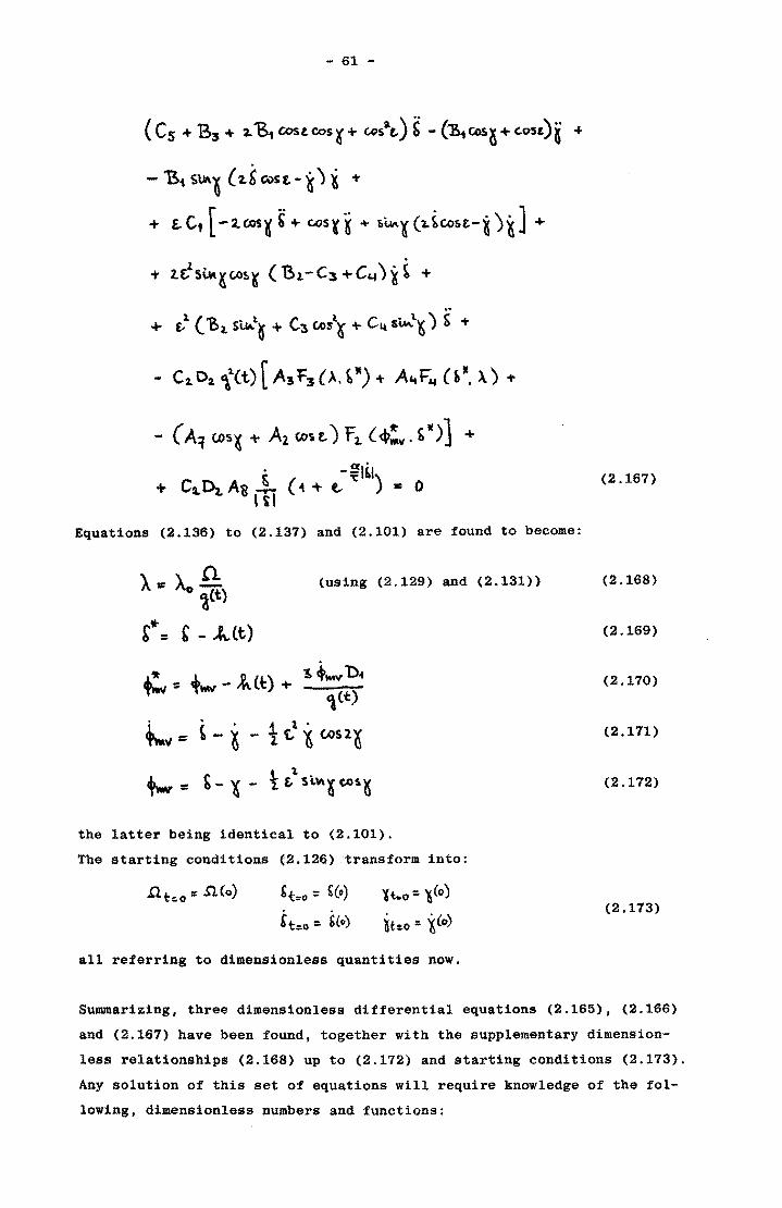
- 61 -
(cs +B3+ 2.151cost.Cos~+GOS1c.)~ -('B1CoS~+C.O")~ ...
- 'Bi SU\l (2.~ cost. - i) i i"
+ £. C, [ - 2.GOSK G + c.os¥ K + \\.IA'( (l.~cost- ~ )~] +
i' 2.&lst"'~~~ ('B1-C3 +c~) i t +
... £,1 ("B~ Sw.l~ + C3 (A)S<~ + Cit S"""l.~ ) & i"
- (A1 (.OS,( + A2 COS t. ) Fl. (<l>!V . t")] +
. -gl'l + C:&.Dl. Ai ~ (-1 + t.. "C ) • 0
I t I
Equations (2.136) to (2.137) and (2.101) are found to become:
A= >..~) (using (2.129) and (2.131»
.. t = ,- ..l(t)
+:v::: +-r - ~(t) + 1> +tMV 1)1 ,et )
+-\1:: t - ~ - t {..t i ~s 2 G
the latter being identical to (2.101).
The starting conditions (2.126) transform into:
't.,o = 'Co)
tt::.o:; &(0)
It.o:; leo)
~tc:o ::. ~(o)
all referring to dimensionless quantities now.
(2.167)
(2.168)
(2.169)
(2.170)
(2.171)
(2.172)
(2.173)
Summarizing, three dimensionless differential equations (2.165), (2.166)
and (2.167) have been found, together with the supplementary dimension
less relationships (2.168) up to (2.172) and starting conditions (2.173).
Any solution of this set of equations will require knowledge of the fol
lowing, dimensionless numbers and functions:
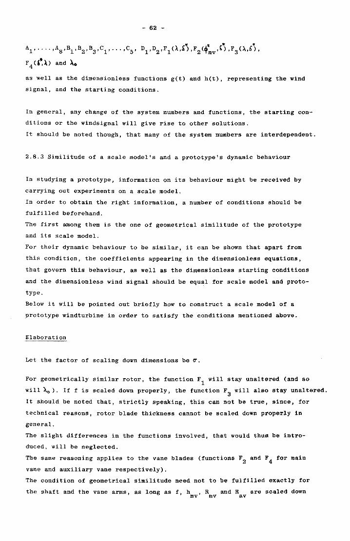
- 62 -
.. It (''II: ,.
Al'····,AS,Bl'B2·Ba'Cl'····CS' Dl'D2'Fl(l.~).F2('mv·~),Fa(X,&),
F 4 ( ,~ ).) and ).0
as well as the dimensionless functions g(t) and h(t). representing the wind
si.gnal. and the starting conditions.
In general. any change of the system numbers and functions. the starting con
ditions or the windsignal will give rise to other solutions.
It should be noted though. that many of the system numbers are interdependent.
2.8.a Similitude of a scale model's and a prototype's dynamic behaviour
In studying a prototype, information on its behaviour might be received by
carrying out experiments on a scale model.
In order to obtain the right information, a number of conditions should be
fulfilled beforehand.
The first among them is the one of geometrical similitude of the prototype
and its scale model.
For their dynamic behaviour to be similar, it can be shown that apart from
this condition, the coefficients appearing in the dimensionless equations.
that govern this behaviour. as well as the dimensionless starting conditions
and the dimensionless wind signal should be equal for scale model and proto
type.
Below it will be pOinted out briefly how to construct a scale model of a
prototype windturbine in order to satisfy the conditions mentioned above.
Let the factor of scaling down dimensions be ~.
For geometrically similar rotor, the function Fl will stay unaltered (and so
will Ao). If f is scaled down properly, the function Fa will also stay unaltered.
It should be noted that, strictly speaking, this can not be true, since, for
technical reasons. rotor blade thickness cannot be scaled down properly in
general.
The slight differences in the functions involved, that would thus be intro
duced. will be neglected.
The same reasoning applies to the vane blades (functions F2 and F4 for main
vane and auxiliary vane respectively).
The condition of geometrical similitude need not to be fulfilled exactly for
the shaft and the vane arms, as long as f, h ,R and R are scaled down mv mv av
- 63 -
properly. Small deviations from the original design will not affect the cor-
respondence seriously.
M is scaled down by o
-3 IT ,since it is proportional to the pump's piston area
(a-2
) and the pump's -1 crank arm (a ) .
Then from (2.130) it is seen that V is equal for prototype (PT) and scale o
model (8M).
For Al (2.140) to be equal for PT and SM, dx
should be reduced bya-3
This
turns out to be automatically the case, when the rotor is scaled down in twa
dimensions (aspect dimensions; blade thickness unchanged). I is then found x
to fall down to a-4 of its original value.
The following dimensionless numbers are now easily seen to stay unchanged in
scaling down: A2 ,A3
,A4
and A7
.
For SM D2 is found to become IT times as great as for PT, since by (2.129)
o =Q.a (!), while ~x(2.128) is found not to change. The product of D2 °SM OPT
and C2
appearing in the differential equations (2.166) and (2.167) should
however be equal for PT and SM, so that I s
3 should be reduced by a factor IT
Inspection of A5,A6,B1,B2,B3 C1
'C3 and C4 shows that the following main vane 3
parameter products, should, like I j all be scaled down by a factor a : s
GR g
mR2 g
mb2 g
mbR g g
d s
This might be accomplished by a suitable choice of materials. If these conditions
are found to be impossible to meet simultaneously, compromises will have to
be made for sheer necessity.
As for D1 , it is seen to become a times as small for 8M as for PT. In other
words, within the choices made here, it is impossible to scale down the proto-
type in such a manner that the main vane's 'aerodynamic damping' is not spoiled. 3 From (2.155) it is seen that I should be reduced by a factor a ,
z as should d z
in (2.147), which might again be accomplished by a suitable choice of materials.
Further the dimensionless input signals get) and h(t) should be equal for 8M
and PT.
Finally. the starting conditions (2.173) should be equal for 8M and PT. Note
that for SM, nt=O (non-dimensionless) should be given a value cr times as great
as for PT.
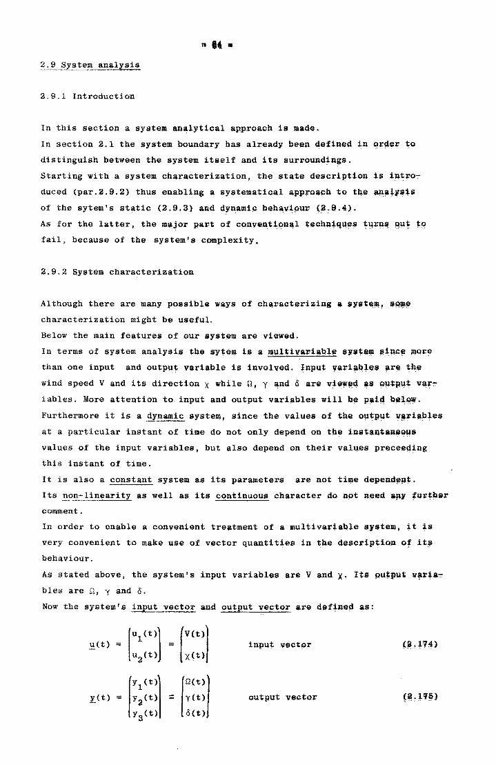
2.9 System analysis
2.9.1 Introduction
In this section a system $llalytical approach is made.
In section 2.1 the system boundary has already been defined in order ~o
distinguish between the system itself and its surroundings.
Starting with a system characterization, the state description is intro
duced (par.2.9.2) thus enabling a systematical apPfoa~h to tn.e ~~t'~~S
of the sytem's static (2.9.3) and dynamic beh~yiour (?9.4).
As for the latter, the major part of cQnyen~ional techniques tHr~~ 8~t to fail, because of the system's complexity.
2.9.2 System characterization
Although there are many possible ways of characterizing a sYite~, s9~~
characterization might be useful.
Below the main features of our system are viewed.
In terms of system analysis the sytem is a multivar.iab,le syst;elll sin/!~ !'lore
than one input and output variable is involved. Input variab,les ar~ ~~e
wind speed V and its direction X while n, Y aqd G are vi~w~d as OH~PHt v~r~ iables. More attention to input and output variables will be Paip be~ew~ Furthermore it is a dynamic system, since the values of the output v~riables
at a particular instant of time do not only depend on the instantaneoHS
values of the input variables, but also depend on their values precee~tng
this instant of time.
It is also a constant system as its parameters are not time depend~~t.
Its non-linearity as well as its continuous character do not n~ed ~P1 'u~t~er
comment.
In order to enable a convenient treatment of a multi variable s1_tam, it ~s
very convenient to make use of vector quantities in the description of its
behaviour.
As stated above, the system's input variables are V and X~ Its Qu~put v~~~a~
bles are ~, Y and o. Now the system's input vector and output vector are define~ as:
[U1 (t)j rV(t)] ~(t) = =
u2(t) X(t)
input vector ~~L 114)
['1 (t)1 rt)j x..(t) = Y2(t) :- yet)
Y3(t) oCt)
output vector
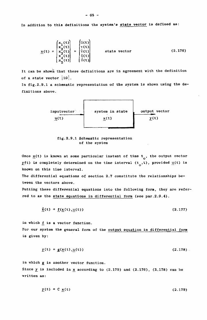
- 65 -
In addition to this definitions the system's state vector is defined as:
state vector (2.176)
It can be shown that these definitions are in agreement with the definition
of a state vector 1101.
In fig.2.9.1 a schematic representation of the system is shown using the de
fini tions above.
input vector .. system in state
E.(t) ~(t)
fig.2.9.1 Schematic representation of the system
output vector
L(t)
Once ~(t) is known at some particular instant of time t , the output vector o
_y(t) is completely determined on the time interval (t ,t), provided u(t) is o -
known on this time interval.
The differential equations of section 2.7 constitute the relationships be
tween the vectors above.
Putting these differential equations into the following form, they are refer
red to as the state equations in differential form (see par.2.9A).
(2.177)
in which f is a vector function.
For our system the general form of the output equation in differential form
is given by:
(2.178) .
in which £ is another vector function.
Since 1. is included in ~ according to (2.175) and (2.176), (2.178) can be
written as:
l.(t) = C ~(t) (2.179)
- 66 -
in which C, the output matrix is given by:
C = I~ ~ ~ ~ ~l o 0 0 1 0
(2.180)
(2.177) and (2.178) together constitute the system equations.
2.9.3 Static behaviour
The system's static behaviour is defined as the set of solutions L(~) to
the system's static equations. The latter are found by putting all time de
rivatives of x to 0 in the system's differential equations.
Since, for clear reasons, X is not involved in static behaviour, the system's
static behaviour is given by L(Ul):
= [~~~~l o(V)
(2.181)
Solving the static equations requires the use of special techniques since
they are coupled and non-linear. One of them is the generalized Newton-Raph
son method 121. .
A more easy and reliable method is suggested at the end of section 3.4.
2.9.4 Dynamic behaviour
The system's dynamic behaviour is governed by the three, non-linear and coup
led differential equations of section 2.7, one of which is of first order and
two of second order.
It is defined as the behaviour performed by the system when it is not in a
state in which x3=x
5=O, see (2.176)
In order to obtain quantitative information on this dynamic behaviour and in
particular the system's stability properties, the equations in differential
form (2.177) may be linearized near such a state.
As a first attempt this is done for £=0 (except in M (G) for clear reasons) s
and for u2
=X=0 (constant wind direction).
With £=0 the differential equations of section 2.7 transform into:
(2.182)
" .. .. 2 I y-(mh R +1 )o+mh R sinyo +M (G)+D -M (Fmv> = 0 s g g s g g s s s
(2.183)
2" . (I +mh +2mh R cosy+I )o-(mh R cosy+I )y-mh R siny(2o-y)y+
z g g g s g g s g g
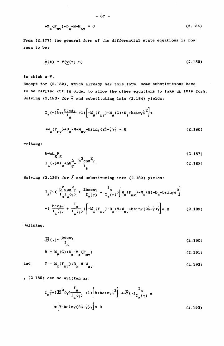
- 67 -
+M (F )+D -M-M = 0 z mv z av (2.184)
From (2.177) the general form of the differential state equations is now
seen to be:
i(t) ::: f(!.(t) ,u) (2.185)
in which u=V.
Except for (2.182), whic,h alreidy has this form, some substitutions have
to be carried out in order to allow the other equations to take up this form.
Solving (2.183) for y and substituting into (2.184) yields:
writing:
.. bcoey [ ,2] I (y)'+( I .+1) -M (F )-M (G)+D +bsinyc +
z s mv s s s
+M (F )+D -M-M -bSiny(25-y)y = 0 z mv z av
b=mh R g g
2 I (y):::I +mh -
z z g
..
2 2 b cos Y
I s
Solving (2.186) for 0 and substituting into (2.183) yields:
Defining:
and
.::B(y): bcosy I
s
W = M (G)+D -M (F ) s s s mv
Y = M (F )+D -M-M z mv z av
, (2.189) can be written as:
(2.186)
(2.187)
(2.188)
(2.189)
(2.190)
(2.191)
(2.192)
(2.193)
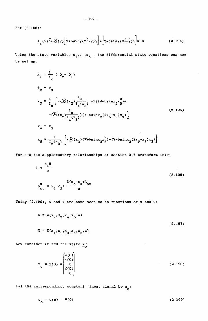
- 68 -
For (2.186):
(2.194)
Using the state variables x1 , ... x5
' the differential state equations can now
be set up.
1 ( Qr- Ql) xl =
I x
x2 = x3
I
x3 = [-(~(X2)Iz~X2) +1)(W+bSiDX2X:)+ I s I
-(lS(X2)Iz~X2)}(Y-bSinX2(2X5-X3)X3)] (2.195)
x4
:: x5
1 [-13 (X2 ) (W+bSiDX2X!>-(Y-bSinX2(2X5-X3)X3)] Xs = I z (X2
)
For 8=0 the supplementary relationships of section 2.7 transform into:
lIE
<Pmv
u
Using (2.196), Wand Yare both seen to be functions of x and u:
Now consider at t=O the state x : -0
~ = ~(O) =
0(0) yeO)
o 0(0)
o
Let the corresponding, constant, input signal be u : o
U :: u(o) = V(O) o
(2.196)
(2.197)
(2.198)
(2.199)
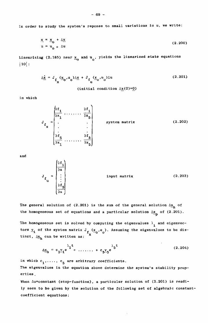
- 69 -
In order to study the system's reponse to small variations in u, we write:
x = x + t;~ -0
U = U + t.u o
(2.200)
Linearizing (2.185) near ~ and uo
' yields the linearized state equations
110 1 :
Jf
(x ,u )t.x + Jf
(x ,u )t;u -00- -00
(2.201) X U
(initial condition t;~(O)=Q)
in which
af1 af1
aXl .............
aX5
Jf = system matrix (2.202)
x
di5 df5
aXl ..............
dXS
and
= input matrix (2.203)
The general solution of (2.201) is the sum of the general solution t;~h of
the homogeneous set of equations and a particular solution t;x of (2.201). -p
The homogeneous set is solved by computing the eigenvalues A. and eigenvecJ.
tors Yi of the system matrix Jf
(~,uo)' Assuming the eigenvalues to be dis-
tinct, ~~h can be written as: x
(2.204)
in which c1 ' .... , 0 5 are arbitrary coefficients.
The eigenvalues in the equation above determine the system's stability prop
erties
When ~u=oonstant (step-function), a particular solution of (2.201) is readi-
ly seen to be given by the solution of the following set of algebraic constant
coefficient equations:
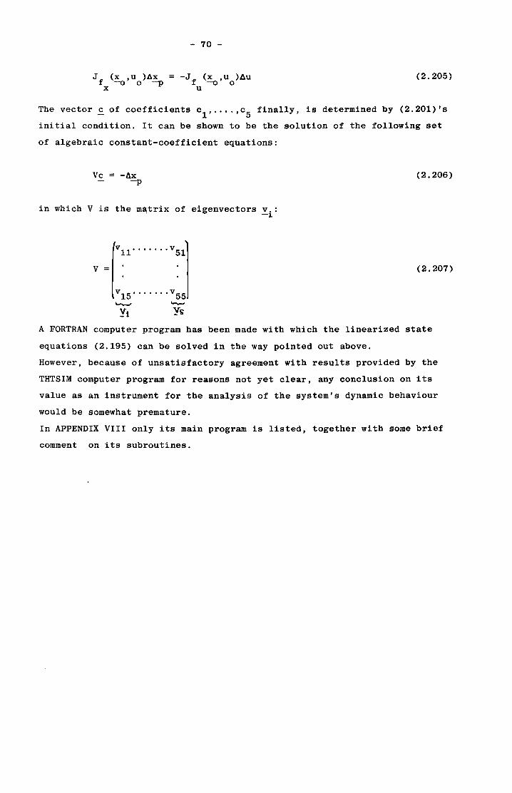
- 70 -
Jf
(x ,u )~x = -Jf
(x ,u )Au x-o 0 --p U-o 0
(2.205)
The vector c of coefficients c1
' ..•. ,c5
finally, is determined by (2.201)'s
initial condition. It can be shown to be the s.olution of the following set
of algebraic constant-coefficient equations:
Vc = -Ax --p
in which V is the matrix of eigenvectors v.: -~
V !Vll ....... v 51
= V~5 ••••••• V~5 ~ .......... Yt Ys
(2.206)
(2.207)
A FORTRAN computer program has been made with which the linearized state
equations (2.195) can be solved in the way pointed out above.
However, because of unsatisfactory agreement with results provided by the
THTSIM computer program for reasons not yet dlear, any conclusion on its
value as an instrument for the analysis of the system's dynamic behaviour
would be somewhat premature.
In APPENDIX VIII only its main program is listed, together with some brief
comment on its subroutines.
- 71 -
III Computer simulation.
3. 1 Introduction.
For evaluating the steady-state behaviour of windmi,lls with mecha.ni.cal safety
and control systems there exist sev~ral analysts. See f.i. 111,121
These programs give results confirmed in windtunnel tests. However the dynami
cal behaviour of these windmills in the field gives rise to many questions.
It was decided therefore that the developing of a computer program that could
predict the dynamical behaviour of such a system was of great interest.
A program like that could be used to see whether a system is uneasy or un
stable and how this is influenced by changing of system parameters meanwhile,
of course, without letting go of the safety qualities. It can also give an
impression of the power output under fluctuating wind conditions.
In this chapter we will deal with some information on continuous simulation
language and programs, with THTSIM, the language we used, and the general
outline of a windmill simulation program.
3.2 Computer simulation of physical models.
Computers are systems designed to implement mathema,t:i,caJ relationships. These
can be idealized relationships of a physical model.
One application of computers, computer simulation, substitutes a computer Im
plemented model for real system components in experiments conducted for pur
poses of design, training or partial tests.
Convention~y computers are classified as Analog computers when the machine
variables are considered to vary continuously and as Digital computers when
they are discrete-state systems. Hybrid computation is a technique to combine
the advantages of both Analog and Digital computation. An advantage of Analog
computation is the high computation speed. Advantages of Digital computers
are accuracy and memory storage.
WhatE!ver kind of computer is chosen, for simulation an idealized mathematical
model of the system in study has to be set up_
The great use of simulation programs is the ease to change system parameters
or input signals and to no~ce the changes in behaviour that occur. To do so
in reality would be laborious and expensive.

- 72 -
3.3 tilly use THTSIM?
We thought it toolaborious to develop our own continuous computer simulation
language. Though it would be pos to do so in FORTRAN, the aim of our
work was not to become a specialist in computer languages but to simulate
the behaviour of windmills. When looking for a simulation language THTSIM
was recommended for our purpose. THTSIM is a language for interactive simu
lation of continuous and hybrid systems on a PDP 11 minicomputer \ISI (Di
gital computer)
A PDP 11 computer was available for use in a nearby physical laboratory of
the UvA. THTSIM appeared to be very easy to handle especialy because of the
block diagram notation familiar with a notation for analog computation in
use at UvA and part of our curriculum.
In spite of some shortcomings of THTSIM, see section 3.5, we have continued
to work with it.
3.4 Properties of THTSIM.
As stated before, THTSIM is a language for interactive simulation of conti
nuous systems. Floating point arithmetic is used requiring no scaling. The
model can be specified in block diagram form (or, but of no importance to
us, in bond graph form or a free mixture of both).
Advantages are the interactive character of the language and the floating
point arithmetic.
A THTSIM program consists of four sections:
I. Structure
2. Parameters
3. Plotblocks
4. Timing.
The structure contains in block diagram notation the differential equations
governing the system and all other mathematical relationships.
The section parameters contains all additional information on the system
such as initial values, constants and gain factors, data points that provide
functions etc.
The section plotblocks contains the information on what variables are desired
as output and on what scale they are to be plotted.
- 73 -
The section timing contains the integration step size and the end time of the
simulation run.
To form the structure of a program the mathematical relations have to be re
written in block diagram form. For this all kinds of blocks are provided.
Blocks for mathematical operations such as adding (SUM), multiplying (MUL,
GAI(n) or ATT(enuate» and integration (INT).
Blocks for mathematical functions as sine (SIN), square root (SQT), logarithm
(LOG), absolute value (ABS) etc.
There are blocks to create functions by stating data points (FNC) and to fetch
data points from file (DAT).
There are blocks for convenient handling of a lot of problems. For an exhaustive
list see the users manual \15'1
Every loop in a THTSIM structure must at least contain one so-called history
block, such as an integration block. If this condition is not met naturally
it c,m be met by introducing an algebraic delay block (AnL).
To give an idea of the use of THTSIM the user's manual example is copied here,
see fig 3.1. The command "SD" at the end of the illustration means: Start si
mulation, output on display.
A list of commands is at hand to start and terminate programs, change sections,
list the program, file manipulation etc.
A print-plot can be made showing at most four variables at a time plotted
against time. This is done by stating the variable numbers and their scales.
In the example the symbol "0" stands for time. Time on the horizontal axis
can be replaced by any optional variable to plot variables one against each
other. Beside output in the form of a print plot on a display a numerical
output can be obtained by the command "SNit. Here the maximum amount of output
variables is five.
Output can be stored on file and used again in a later run.
The program can be interupted at any time and proceded afterwards, if neces
sary 'N'ith calling the actual values of variables of interest.
Some t=xamples of programs that can be made are:
The response of a system (windmill) to an increase of the windspeed or a varia
tion of the wind direction.
The rHsponse of a system on sine or triangle windspeed variations of different
frequencies in order to test oscillatory modes.
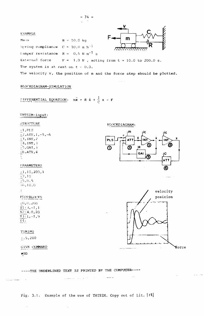
- 74
l::XAMPLE ---~,~--
F Mi:I~;s m 10.0 kq
;';f,r.ing cnmpliance C 10.0 10 N- 1
I·c\lllper resistance R 0.') N 10- 1 s
Ext.erndl force F 1.0 N , acting trom t 10.0 to 200.0 s.
The syst.em is at rest on t '"' 0.0.
The velocity v, the position of rn and the force step should be plotted.
BLOCKDIAGRAM-SIMULATION
]; [FFERENT IAL EQUATION:
:r:~i'I'S IM- input:
STRUCTURE
:l,PLS : 2,ATT, 1,-5,-6 -=-3,INT,2 : 4, INT, } : S,GAI, 3 :..6 ,ATT ,4
PARAMETI<;RS
-=-1,10,200,1 : 2,10 : ':' I (). ')
: n, 1 (). ()
PI ,( )'J'BLOCKS ~ ...... ------.-:0,0,200 ~1_:_ J , - 1 , 1 Y2:4,O,20 Y3: ,-1,9 Y,1 :
TIMING
:.5,200
(; 1 Vl': t~OMMAND
#SD
1 mx + R x + - x = F
C
BLOCKDIAGRAM:
--_ ..... __ .
I velocity
position .. /<~'.
----THE UNDERLINED TEXT IS PRINTED BY THE COMPUTER----
Fig. 3.1. Example of the use of THTSIM. Copy out of Lit. Ilsl
oree
- 75 -
Th8 response of a system on a reallike windsignal.
Modifications can be made and the changes in behaviour can be made visible.
Ultimately also steady state points for different windspeeds can be calcu
lated by offering the system a constant wind signal for a longer period.
3.5 Some restrictions of THTSIM.
After discussion of the qualities of THTSIM we here state some of the res
trictions of this computer language. Some of them concern input and output
facilities and some concern the tools to build a program, so the missing
of certain blocks.
First some input/output comments.
I. No command is available for a selective listing of a part of the program.
The command "Lit gives a listing of the entire program with inclusion of all
data in function blocks and the statements that run the program, plotblocks
etc. For a short program this is not a problem but for a program of about 400
blocks with extensive function blocks among them such a listing consumes much
time and paper.
Pricipally block numbers can be used without any logical order in the num
be~s. This was told us to be the reason for not having a selective listing
command. However we built the program in such a manner that clusters of
block numbers perform certain sub programs. It would therefore be very con
venient to be able to list only a specified part to check its structure thereby
suppressing of all data figures involved.
2. It is impossible to list more than five output variables simultaneously.
We have found that to little in some cases. If one wants more output varia
bles the program has to be run again.
3. There is no possibility of adding text to the program, no title, nor ex
planations or comments.
Comments on the complete set of blocks available are:
A. We seriously missed a function block to compose a function of more than
one variable. THTSIM is equipped with a FNC block that, provided with data
points (X,Y), gives a continuous function of X by means of interpolation
among the data points. However for functions of two variables such a block
is not present. We had several functions like that, f.i. C = C (A,t). With q q
use of other blocks this problem can be overcome but it requires a lot of
work. Some examples of how this can be solved are given below.
- 76 -
AI. Say F = F(A,B). Evaluate the functions F ~ F(A) for equidistant values of
B. Put these functions in function blocks (FNC) and build a linear interpolator
for intermediate values of B. A scheme of this type of solution is given in
Appendix IX
A2. Evaluate one function (£.i. F = F(A,O» for one value of B and calculate
the factors to multiply this function by for other values of B and chosen
values of A. Evaluate the coefficients of the function f = a+bB+cB2+dB3 •••
that represent these factors as accurate as wanted for the chosen values of
A. Then all coefficients a,b,c ••• are to be put in function blocks as a func
tion of A and f is evaluated for intermediate values of A. By multiplying the
base function with f the function F = F(A,B) is evaluated. A scheme of this
procedure can be found in Appendix IX
A3. Tricks and treats with analytical functions in combination with one of
the above mentioned methods;,
B. THTSIM is provided with a relais switch that chooses one desired input
out of three possible input in respons of a fourth input. We missed a block
working oppositely: In response to one input the other input follows one out
of three branches afterwards. Such a block could be used to call in alterna
tive means of calculation when mathematical problems might arise, such as di
viding by zero. The provided blocks require that all branches of the program
can be calculated. This is done first. After that a choice is made. In some
problems it would be more convenient to first choose a branche and than cal
culate it, somewhat like the FORTRAN "IF" statement.
c. A possibility to reset a block to its initial value during the program run
if a certain condition is met is not present.
D. An algebraic delay with a variable delay time as function of a second in
put variable. (Though we recognize the problems for this one).
.... 77-
3.6 General outline of the computer program for windmill simulation.
This section is meant to give a general view of the computer program for
simulation of a wind turbine. Therefore it will make use of the differen
tial equations that govern the behaviour of a windmill with a mechanical
control system such as derived in chapter II. A summary of these differen
tial equations and other relations that have been made is given in sec
tion 2.8.
A detailed discussion of the computer program will be given in chapter IV.
The reader who is not interested in such a detailed discussion can jump
forward to chapter V after this section.
The system is one with three rotational degrees of freedom, thus the THTSIM
program is. in essence, a set of three coupled differential equations of
the form:
angular acceleration = L • torque I Moment of inertia . ax~s ax~s
and consecutive integrations
The equations describe motion of the rotor about the X-axis, motion of the
shaft + main vane + rotor about the Z -axis and motion of the main vane o
about the S-axis (inclined hinge axis).
The equations of section 2.7 can be written as follows: . ~ = {-Q - D + Q } I I
~ x r x 3.1
6 == {M + M - M (F ) - D + R } I It av z mv z z z 3.2
y = {M (F ) - M (G) - D + R } I I s mv s s s s 3.3
Fig. 3.2 shows a general outline of the computer program. The calculations
of the angular accelerations, velocities and displacements can be found in
the third column. In the left margin the three axes are indicated. The
numbers in fig. 3.2 refer to block numbers in the actual THTSIM program.
The right-hand sides of the equations 3.1 to 3.3 contain parameters and
functions of a specific turbine. They can be distinguished. besides a di
vision according to the axes, after their nature:
-The aerodynamical torque Q and the aerodynamic moments M, M (F ), M (F ) r zmv smv and M • av
-The gravitational moment M (G). s
- 78 -
-The dissipative moments Ql' D ,D and D x z s
-The moments due to mutual interaction, Rand R z s
-The moments of inertia about the three axes I , I' (the accent denoting that x z
the term is not a constant) and I . s
In the general outline the moments can be found in the second column, ex
cept for the moments of inertia. In the computer model all right-hand
terms of 3.1-3.3 have to be evaluated. This is done by stating all parame
ters and providing all necessary functions. The initial values of angular
velocities and angular displacements have to be set. Finally the last fune
tions, windspeed and wind direction, the major input variables, have to be
stated. They are represented by hexagonal blocks in fig. 3.2.
The velocities and positions are calculated by integration over a short
period. These supply the information for the next integration step. This
goes on until a certain preset time is met. The chosen output variables
can be made visible on a screen.
For reasons of clearness several feedbacks and crosslines between axes
are omitted in this scheme 3.2 but they can be traced by looking at the 1n
puts of the second column. Each integration step this program is run from
left to right and restarted with the newly calculated values.
Each of the blocks in this general outline will be dealt with in detail
in chapter IV. There the discussion will follow a division based on the
three axes.
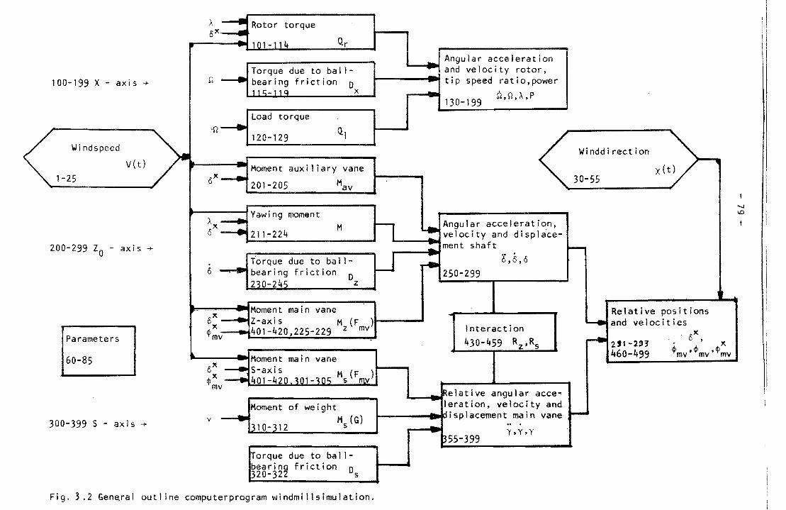
100-199 x - axis ~
Windspeed
A ~ Rotor torque 6x~
101-114 Qr
Torque due to ballf/, ---..j bea ring f ric t ion 0
115-]19 x
Load torque >Q~ Q
1120-129 I
V(t) Moment auxiliary vane x
1-25 6 201-205 Mav
200-299 z -o ax is -+
Ax ----I Yawl ng moment
o ---e-t 211-224 M
o Torque due to ball
""""""bearing friction D 230-2it2 z
I Angular acceleration
~~ .... and velocity rotor, ~--------.~- tip speed ratio,power
~
130-199 Q,Q,A,P
Angular acceleration, velocity and displace
'----.... ment shaft
6,6,6 250-299
Winddirection
30-55
I--
~
x Moment main vane 6 Z-axis M (F )1-----~~v 401-420,225-229 z mv Interaction
430-459 Rz,Rs
Relative positions ~and velocities
Parameters
OX .... ---. ~x v)
60-85
300-399 S - axis -+ y
mv
Moment of weight
~-112 Ms(G)
~orque due to bal 1-bearing friction D 320-322 s
Fig. 3.2 Gen~ral outline computerprogram windmillsimulation.
~ __ ... "r.elative angular acce~ leration, velocity and
r-------~ .. ~~~isplacement main vane .--
~55-399 Y,Y,Y
~2'1-2!H 460-499
oX . ' x 4>mv·4>mv·4>mv
"-I 1.0
- 80 -
IV. Computer model.
4.1 Introduction.
This chapter is meant to give a detailed description of the computer model
for simulation of a windmill with mechanical control system. Section 4.2
lists all the statements of the program with comments and if possible the
mathematical meaning. In the text, numbers between brackets ( ) refer to
block numbers in the program. Underlined numbers refer to constants.
The data points from FNC (function) blocks are omitted. They can be found
in App. XI wich gives a complete listing of the program.
Section 4.3 deals with a 'wind model' that is used in combination with
the main program.
Section 4.4 deals with a problem for the main vane, time delay, that is
not taken in account in the computer model.
Section 4.5 provides some essential remarks about the accuracy of the
computer model.
Section 4.6 finally provides some results of the computer model that are not
dealt with in other sections of this report (See also Chapter V).
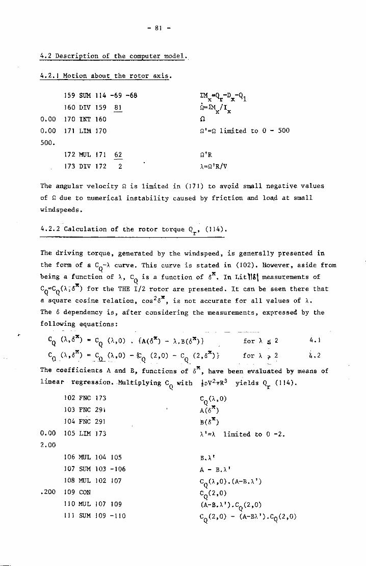
- 81 -
4.2 Description of the computer model..
4.2.1 Motion about the rotor axis.
159 SUM 114 -69 -68
160 DIV 159 81
0.00 170 INT 160
0.00 171 LIM 170
500.
172MUL 171 62 -
173 DIV 172 2
EM -Q -D -Q x r x 1 Q=EM /1 x x fi
Q'=Q limited tq 0 - 500
The angular velocity Q is limited in (171) to avoid small negative values
of Q due to numerical instability caused by friction and lo.a.d at small
windspeeds.
4.2.2 Calculation of the rotor torque Q , (114). r
The driving torque, generated by the windspeed, is generally presented in
the form of a CQ-A curve. This curve is stated in (102). However, aside from
being a function of A, CQ
is a function of ox, In Litll8\ measurements of
CQ"CQ(A;15X) for the THE 1/2 rotor are presented. It can be seen there that
a square cosine relation, cos 215x , is not accurate for all values of A.
The 0 dependency is, after considering the measurements, expressed by the
following equations:
CQ (A,Ox) ~ CQ (A,O) . {A(ox) - A.B(6x)}
x x C <)( A , a ) - C1L ~~, 0) - {C Q (2, ° ) - C Q ( 2 , a )}
for A ~ 2
for A ?' 2
4. ]
~.2
The coefficients A and B, functions of ox, have been evaluated by means of
linear regression. Multiplying CQ
with. iPV2 1TR3 yields Qr (114).
102 FNC 173 CQ(A,O) )03 FNC 291 A(ox)
104 FNC 291 B(ox)
0.00 105 LIM 173 At-A limited to 0 -2.
2.00
106 MUL ] 04 105 B.A' ]07 SUM 103 -106 A - B.A' 108 MUL 102 ] 07 CQ(A,O).(A-B.A')
.200 109 CON CQ(2,O)
110 MOL 107 109 (A-B.A').CQ(2,0) 111 SUM 109 -110 C
Q(2,O) - (A-BA').CQ(2,O)
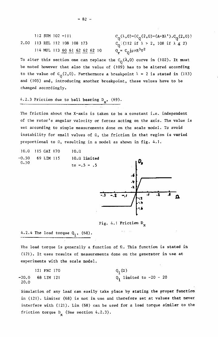
- 82 -
112 SUM 102 -1 II
2.00 113 REL 1 12 108 108 173
CQ
(A,0)-{CQ
(2,0)-(A-BA').CQ
(2,0)}
CQ
, (112 if A > 2, 108 if A .s 2)
114 MUL 113 60 61 62 62 62 10 Q = C ~p'ITR3V2 r Q
To alter this section one can replace the CQ(A,O) curve in (102). It must
be noted however that also the value of (109) has to be altered according
to the value of CQ
(2,0). Furthermore a breakpoint A = 2 is stated in (113)
and (105) and, introducing another breakpoint, these values have to be
changed accordingly.
4.2.3 Friction due to ball bearing D , (69). x
The friction about the X-axis is taken to be a constant i.e. independent
of the rotor's angular velocity or forces acting on the axis. The value is
set according to simple measurements done on the scale model. To avoid
instability for small values of Q, the friction in that region is varied
proportional to n, resulting in a model as shown in fig. 4.1.
10.0
-0.50 0.50
115 GAl 170
69 LIM lIS
10.n
10.0 limited
to -.5 - .5
-.l -.2 -,I
Fig. 4.1 Friction Dx
4.2.4 The load torque Ql' (68).
.• .D.
The load torque is generally a function of ~. This function is stated in
(121). It uses results of measurements done on the generator in use at
experiments with the scale model.
-20.0 20.0
121 FNC 170
68 LIM 121
Q1
(Q)
Q1
limited to -20 - 20
Simulation of any load can easily take place by stating the proper function
in (121). Limiter (68) is not in use and therefore set at values that never
interfere with (121). Lim (68) can be used for a load torque similar to the
friction torque D (See section 4.2.3). x
4.2.5 The power output. - 83 -
The instantaneous power, transferred to the load, is calculated in (130).
The total work done is calculated by integration of (130) in (131). Divi-
ding by time (20) yields the average power transferred to the load. To cal
by the load, all these figures have to be multiplied culate the net work done
by the load's efficiency.
130 MUL 68 170 QI·n 0.00 131 INT 130 Total work done
132 DIV 131 20 Average power output
4.2.6 Motion about the Z -axis and S-axis. o
The shaft and the main vane form a coupled system. The motion about the
Z -axis is expressed in 0, being the position of the shaft relative to a o fixed reference axis, ~ and 8. OX is the position of the shaft relative
to the wind direction. The motion about the S-axis is expressed in y, be-. ing the main vane's position (relative to the shaft), y and y. (There is
no yX). From 0 and y the position of the main vane relative to the reference
axis, ~ ,can be found as well as the position of the main vane relative mv
to the wind direction, ~x • Because of this coupled system, the moment of mv
inertia about the Z -axis is not a constant but a function of the position o
and motion of the main vane. It will be called I'. Also the interaction z
terms Rand R occur as a result of motion about each of the axes. A des-z s
cription of them can be found in section 4.2.14 Interaction.
The function of the two relays (261,263) will be explained in section
4.2.11. They switch as function of the logic 'AND' (241) which is, most
of the time, zero.
0.50
-10.0
0.50
0.00
0.00
0.00
0.00
57.3
250 SUM 203 208 223 -228 448
259 SUM 234 250 -79
260 DIV 259 438
261 REL 262 262 260 241
262 GAl 270
263 REL 233 270 270 241
264 ADL 261
265 ADL 263
270 INT 261
280 INT 263
281 GAl 280
290 SUM 280 -32
E'M =M +'blocking'+YrM (F )+R zav zrnv z
EM = D +E'M -D' z z z z 8= EM /1' z z ;5 (if (241 )=0, (262) othe-rwise, see sec. 4.2.11 also)
-10.t to reset (270)
6 (if (241)=0, (233)=0 otherwise, see ~ec. 4.2.11 also) ADL 0 To avoid algebraic loops
ADL 8 to avoid algebraic loops
o o IS in degrees
ox= 0 - X
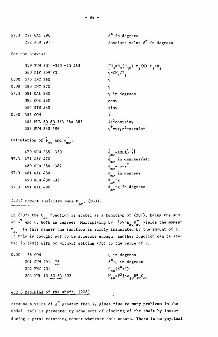
57.3 291 GAl 290
292 ABS 291
For the S-axis:
359 SUM 301 -310 -75 455
360 DIV 359 83
0.00 370 INT 360
0.00 380 INT 370
57.3 381 GAl 380
383 COS 380
384 STN 380
0.50 385 CON
386 MUL 80 80 383 384 385
387 SUM 380 386
Calculation of ~ and mv ¢mv:
470 SUM 265 -370
57.3 471 GAl 470
480 SUM 280 -387
57.3 481 GAl 480
490 SUM 480 -32
57.3 491 GAl 490
- 84 -
4.2.7 Moment auxiliary vane M , (203). av
o'l!: in degrees
Absolute value o'l!: in degrees
EM =M (F )-M (G)-D +R .. ssmv s ss y=D1 /1 . s s y
y
y in degrees
cosy
siny
! h;2cosysiny
Y+=Y+!82coSysiny
¢ =ADL(5-y) mv ~ in degrees/sec
mv + ¢mv= o-y
¢ in degrees mv ¢mv-X
"'mv-X in degrees
In (202) the C function is stated as a function of (201), being the sum av of 6'l!: and ~, both in degrees. Multiplying by !pV2A R· yields the moment av av M . In this manner the function is simply translated by the amount of ~. av If this is thought not to be accurate enough, another function can be sta-
ted in (202) with or without setting (76) to the value of ~.
0.00 76 CON
201 SUM 291 76
202 FNC 201
203 MUL 10 60 63 202
4.2.8 Blocking of the shaft, (208).
~ in degrees
o~+!;; in degrees
C (Q~+!;;) av
M =V2.~pA R* C av av av av
Because a value of o~ greater than ~~ gives rise to many problems in the
model, this is prevented by some sort of blocking of the shaft by intro-
ducing a great retarding moment whenever this occurs. There is no physical
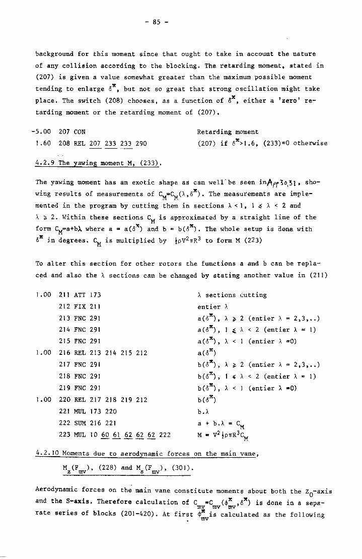
- 85 -
background for this moment since that ought to take in account the nature
of any collision according to the blocking. The retarding moment, stated in
(207) is given a value somewhat greater than the maximum possible moment
tending to enlarge ox, but not so great that strong oscillation might take
place. The switch (208) chooses, as a function of ox, either a 'zero' re
tarding moment or the retarding moment of (207).
-S.OO 207 CON Retarding moment
1.60 208 REL 207 233 233 290 (207) if oX>I.6, (233)=0 otherwise
4.2.9 The yawing moment M, (233).
The yawing moment has an exotic shape as can well' be seen inAfr ~ 0,'31, sho
wing results of measurements of ~=~(A.Ox). The measurements are imple
mented in the program by cutting them in sections A <: t, 1 ~ A <: 2 and
A ~ 2. Within these sections CM is approximated by a straight line of the
form ~.a+bA where a - a(o~) and b = b(6x). The whole setup is done with
OX in degrees. CM is multiplied by ~pV2~R3 to form M (223)
To alter this section for other rotors the functions a and b can be repla
ced and also the A sections can be changed by stating another value in (211)
1.00 2.11 ATT 173 A sections Cutting
212 FIX 211 entier A
213 FNC 291 x a( 0 ), A ~ 2 (entier A = 2,3 ••• )
214 FNC 291 x I A <: 2 (en tier A = 1) a (0 ), ~
215 FNC 291 x a(o ), A <: (entier A =0)
1.00 216 REL 213 214 215 212 a(ox)
217 FNC 29] b(ox), A ~ 2 (entier A :: 2,3, .. )
218 FNC 291 b(ox), " A < 2 (entier A = 1)
219 FNC 291 b(6x), A <: (entier A -0)
1.00 220 REL 217 218 219 212 b(ox)
221 MUL 173 220 b.A
222 SUM 216 221 a + b.A :: CM 223 MOL to 60 61 62 62 62 222 M = V2~p~R3C ----- M
4.2.10 Moments due to aerodynamic forces on the main vane,
M (F ), (228) and M (F ), (301). z mv s mv
Aerodynamic forces on the main vane constitute moments about both the Z-axis o and the S-axis. Therefore calculation of C -C (~x ox) is done in a sepa
mv mv mv' rate series of blocks (201-420). At first ¢x is calculated as the following
mv
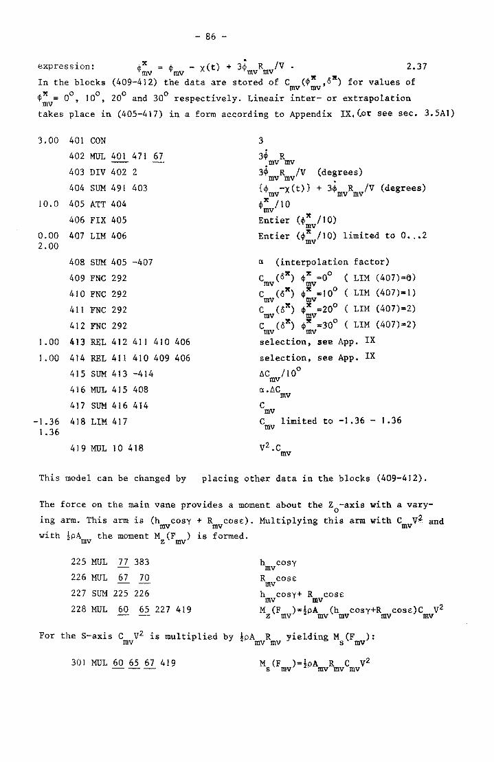
- 86 -
expression: x • / ¢ = ¢ - x(t) + 3$ R V. mv mv mv mv x x 2.37
In the blocks (409-412) the data are stored of C (¢ ,0) for values of mv mv ¢x = 00
100 200 and 300 respectively. Lineair inter- or extrapolation mv • , takes place in (405-417) in a form according to Appendix LX.(pr see sec. 3.5AI)
3.00 401 CON
402 MUL 401 471 67
403 DIV 402 2
404 SUM 491 403
10.0 405 ATT 404
406 FIX 405
0.00 407 LIM 406 2.00
408 SUM 405 -407
409 FNC 292
410 FNC 292
411 FNC 292
4]2 FNC 292
1.00 413 REL 412 411 410 406
1.00 414 REL 411 410 409 406
415 SUM 413 -414
416 MUL 415 408
417 SUM 416 414
-1.36 418 LIM 417 1.36
419 MUL 10 418
3
3~ R mv mv 3$ R /V (degrees) mv mv {¢ -X(t)} + 3~ R /V (degrees) mv mv mv ¢x /10
mv Entier (¢x /10) mv Entier (¢x /10) limited to 0 •.• 2 mv
a (interpolation factor)
C (Ox) ¢x =00 (LIM (407)=0) mv mv
C (ox) ¢x _100 (LIM (407)=1) mv mv
C (ox) ¢x =200 ( LIM (407)=2)
mv mv C (ox) ¢x =300
( LIM (407)=2) mv mv
selection, see App. IX
selection, see App. IX
~c / I 00
mv a.flC mv C mv C limited to -1.36 - 1.36 mv
This model can be changed by placing other data in the blocks (409-412).
The force on the main vane provides a moment about the Z -axis with a varyo ing arm. This arm is (h cosy + R COSE). Multiplying this arm with C V? and mv mv mv with !pA the moment M (F ) is formed.
mv z mv
225 MUL 77 383
226 MUL 67 70
227 SUM 225 226
228 MUL 60 65 227 419 - -
h cosy mv R COSE mv h cosy+ R cose: mv mv M (F )=~pA (h cosy+R cose:)C V2 zmv mvmv mv mv
For the S-axis C V2 is multiplied by iPA R yielding M (F ): mv mvmv s mv
301 MUL 60 65 67 419 M (F )=~pA R C V2 s mv mv mv mv
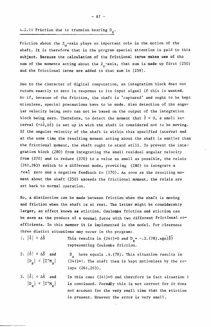
- 87 -
4.2.11 Friction due to trunnion bearing D . z
Friction about the Z -axis plays an important role in the motion of the o shaft. It is therefore that in the program special attention is paid to this
subject. Because the calculation of the frictional terms makes use of the
sum of the moments acting about the Z -axis, that sum is made up first (250) o
and the frictional terms are added to that sum in (259).
Due to the character of digital computation, an integration block does not
return exactly to zero in response to its input signal if this is wanted.
So if, because of the friction, the shaft is 'captured' and ought to be kept
mtionless, special precautions have to be made. Also detection of the angu-
lar velocity being zero can not be based on the output of the integration
block being zero. Therefore, to detect the moment that & = 0, a small in-. . terval (-60,60) is set up in wich the shaft is considered not to be moving.
If the angular velocity of the shaft is within this specified interval and
at the same time the resulting moment acting about the shaft is smaller than
the frictional moment, the shaft ought to stand still. To prevent the inte
gration block (280) from integrating the small residual angular velocity
from (270) and to reduce (270) to a value as small as possible, the relais
(261,263) switch to a different mode, providi~g (280) to integrate a
rea1 zero and a negative feedback to (270). As soon as the resulting mo
ment about the shaft (250) exceeds the frictional m~ent, the relais are
set back to normal operation.
So. a distinction can be made between friction when the shaft is moving
and friction when the shaft is at rest. The latter might be considerably
larger, an effect known as stiction. Coulombs friction and stiction can
be seen as the product of a normal force with two different frtctional co
efficients. In this manner it is implemented in the model. For clearness
three distict situations may occur in the program:
1. 181 > 1:.6
2. 161 < 1:.6 and
IDzl < IE'Mzl
3 . 181 < 1:.8 and
ID 1 < IE'M I z z
This results in (241)=0 and D = -.2.(78).sgn(6) z representing Coulombs friction.
D z
here equals .4.(78). This situation results in
(241)=1. The shaft then is kept motionless by the re-
lays (261,263).
In this case (241)=0 and therefore in fact situation I
is continued. Formauy this is not correct for it does
not account for the very small time that the stiction
is present. However the error is very small.
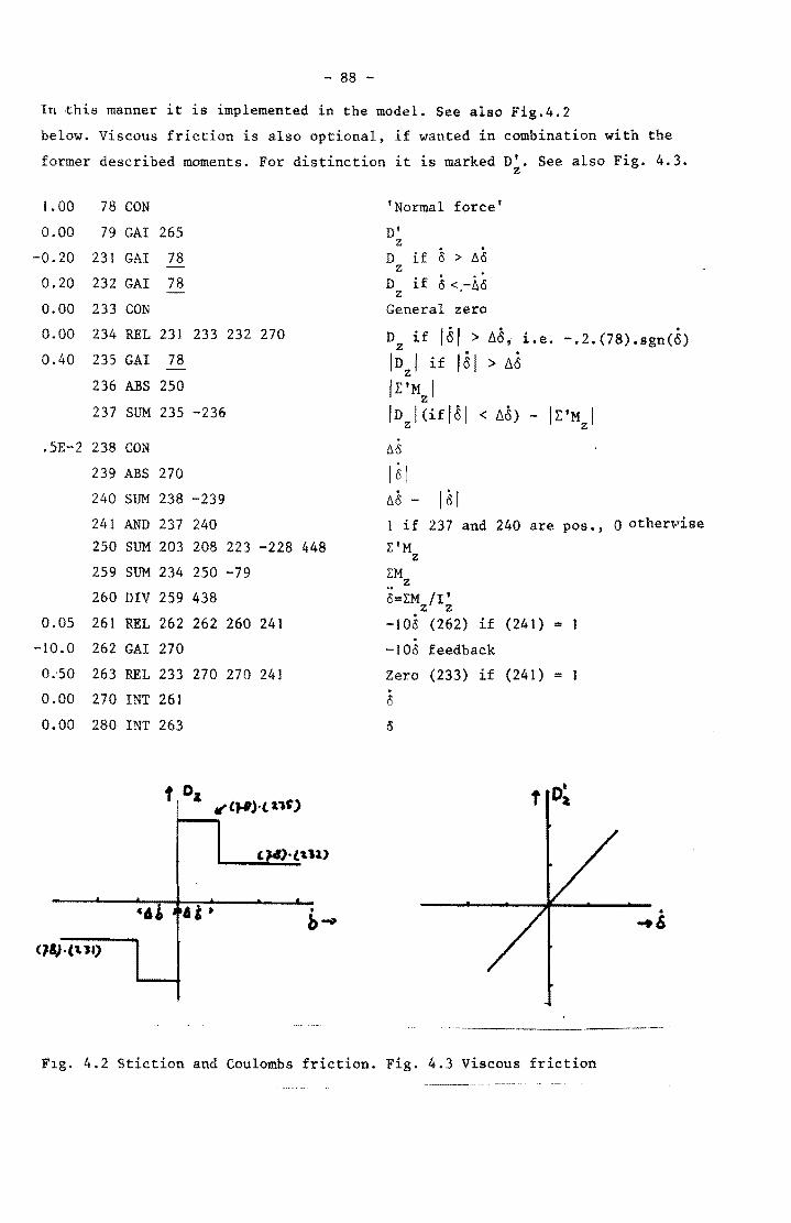
- 88 -
In -this manner it is implemented in the model. See also Fig.4.2
below. Viscous friction is also optional, if wanted in combination with the
former described moments. For distinction it is marked D'. See also Fig. 4.3. z
1.00 78 CON
0.00 79 GAl 265
-0.20 231 GAl 78
0.20 232 GAl 78
0.00 233 CON
0.00 234 REL 231 233 232 270
0.40 235 GAl 78
236 ABS 250
237 SUM 235 -236
.5E-2 238 CON
239 ABS 270
240 SUM 238 -239
241 AND 237 240 250 SUM 203 208 223 -228
259 SUM 234 250 -79
260 DIV 259 438
0.05 261 REL 262 262 260 241
-10.0 262 GAl 270
0~50 263 REL 233 270 270 241
0.00 270 INT 261
0.00 280 INT 263
'1,}.(\ II>
'Normal force'
D' z
D if 8 > 116 z
D if 5 < -68 z
General zero
Dz if I~I > 8d; i.e. -.2.(78).sgn(8)
ID I if 151 > 88 z IE'Mzl ID l(ifl~1 < 86) - IE'M I
Z z
M
161 M - 181 1 if 237 and 240 are pos •• 0 othen1ise
448 L'M z
:MZ
o=LM /1' z z -108 (262) if (241) = . -100 feedback
Zero (233) if (241) = . 6
o
-------------
F1g. 4.2 Stiction and Coulombs friction. Fig. 4.3 Viscous friction
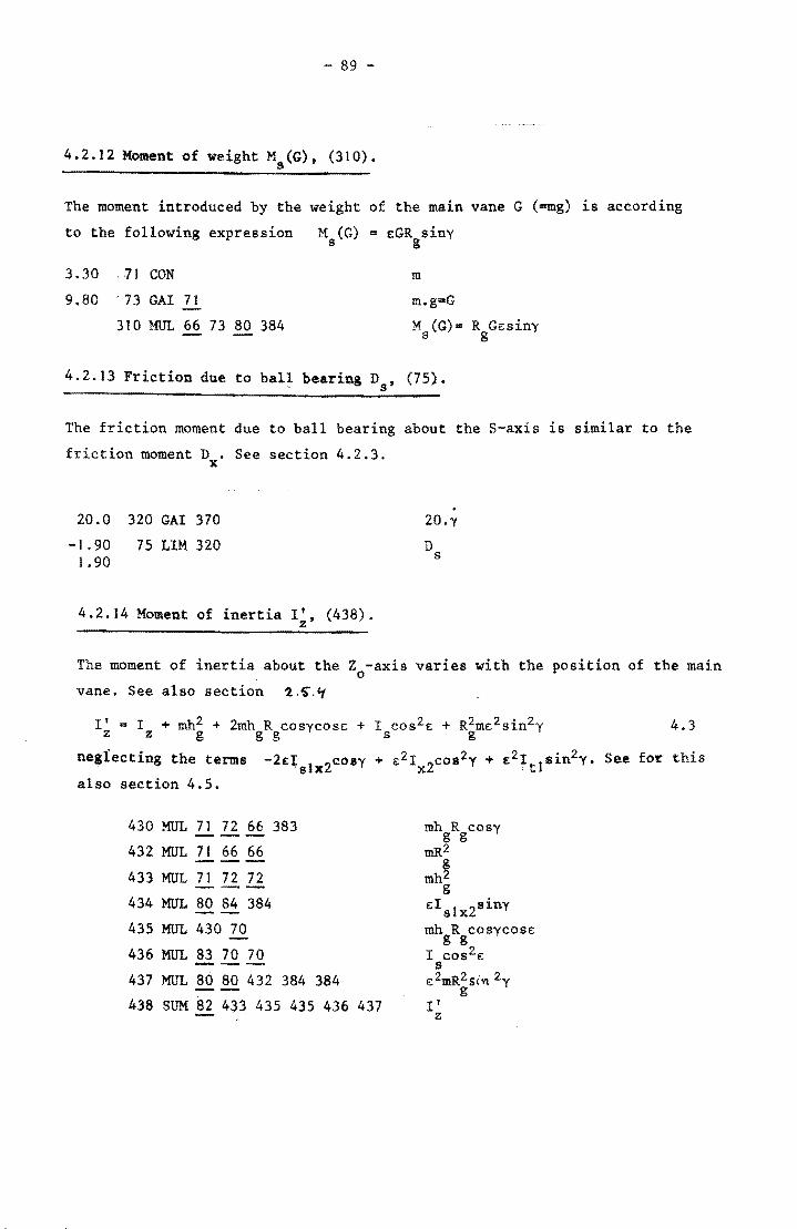
- 89 -
4.2.12 Moment of weight M (G), (310). s
The moment introduced by the weight of the main vane G (=mg) is according
to the following expression M (G) • EGR siny s g
3.30 71 CON
9.80 '73 GAl 71
310 MUL 66 73 80 384
m
m.g=G
M (G)= R Ge::siny s g
4.2.13 Friction due to ball bearing De' (75).
The friction moment due to ball bearing about the S-axis LS similar to the
friction moment D . See section 4.2.3. x
20.0 320 GAl 370
-1.90 75 LIM 320 1. 90
4.2.14 Moment of inertia It z' (438) •
. 20.y
D s
The moment of inertia about the Zo-axis varies with the position of the main
vane. See also section '1.~.'t
It - I + mh2 + 2mh R cosycose:: + I cos2e:: + R2me::2sin2y 4.3 z z g g g s g
11 • 2. 2 • 2 ne$ ectLng the terms -2£lslx2c08Y + £2Ix2co8 Y + £ It1sLn y. See for this
also section 4.5.
430 MUL 71 72 66 383 ---432 MUL 71 66 66
433 MUL 71 72 72
434 MUL 80 84 384
435 MUL 430 70
436 MUL 83 70 70
437 MUL 80 80 432 384 384
438 SUM 82 433 435 435 436 437
mh R cosy g g mR2
mh~ g
d s1x2siny
mh R cosycose:: g g I cos2e::
s e::2mR2si'Vl 2y
g If
Z
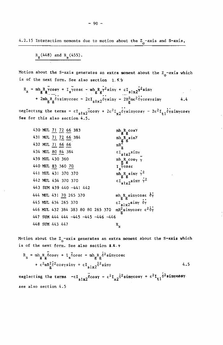
- 90 -
4.2.15 Interaction moments due to motion about the Z -axis and S-axis, o
R (448) and R (455). z s
Motion about the S-axis generates an extra ~roent about the Z -axis which o
is of the next form. See also section 1. ~.Y
R = roh R rcosy + I rcose -roh Ry2siny + 8ISIX2l2siny z gg ... ~~ ___ s gg
+ 2mhgRgoysinycos8 - 28Is1x2 oysiny - 2R~m82Sycosysiny 4.4
neglect1ng the terms - 8Is 1x2YCOSY + 28 2Ix20ysinycosy - 28 2It 18ysinycosy
See for this also section 4.5.
430 MUL 71 72 66 383 mh R cosY --- g g 431 MUL 71 72 66 384 mh R sinY --- ~ g 432 MUL 71 66 66 mR --- g 434 MUL 80 84 384 8Is1x2siny .. 439 MUL 430 360 mh R COSy Y 440 MUL 83 360 70
~ g I yeosE
s 441 HUL 431 370 370 mh R siny ·2 y
g g ·2 442 MUL 434 370 370 8Islx2siny y
443 SUM 439 440 -441 442
444 MUL 431 70 265 370 mh R sinycos8 ~y g g ••
445 MUL 434 265 370 8Is1x2 siny oy
446 MUL 432 384 383 80 80 265 370 mR2sinycosy 82Sy g
447 SUM 444 444 -445 -445 -446 -446
448 SUM 443 447
Motion about the Z -axis generates an extra moment about the S-axis which o
is of the next form. See also section 1.~. ¥
R mh R ~cosy + I 8COS8 - mh R S2sinycos8 s g g s g g
+ 82mR2S2cosysiny + 81 1 282siny g s x
4.5
neglecting the terms -ds1x25cosy - 82Ix2s2sinycosy + 82tt152Sinyeosy.
see also section 4.5
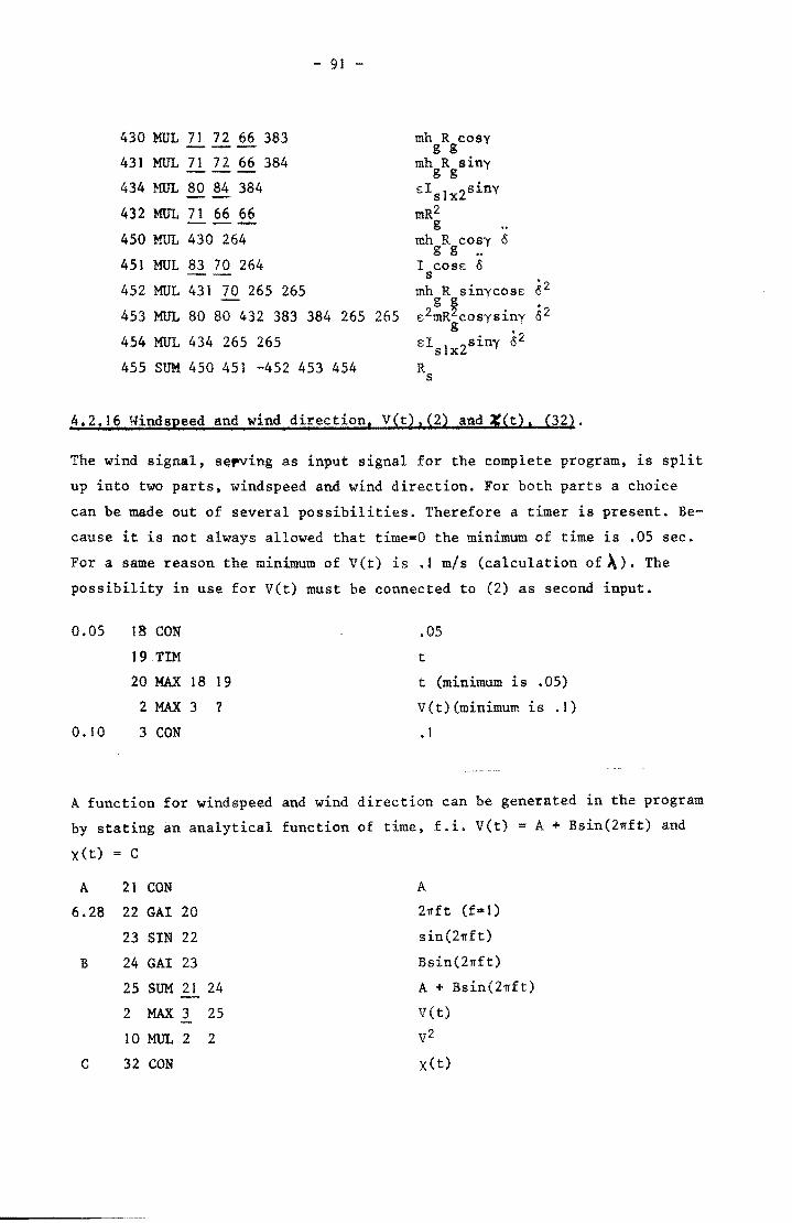
- 91 -
430 MOL 71 72 66 383 mh R cosy --- g g 431 MOL 71 72 66 384 mh R siny --- g g 434 MOL 80 84 384 d slx2siny
432 MOL 71 66 66 mR2 --- g
450 MUL 430 264 mh R cosy 0 g g ..
451 MOL 83 70 264 I COSE: <5 S ~2 452 MOL 431 70 265 265 mh R sinycosE:
453 MOL 80 80 432 383 384 265 265 E:2!R~COsysiny ~2 g •
454 MOL 434 265 265 lx2siny 02
455 SUM 450 451 -452 453 454 R S
4.2.16 tY-indspeed and wind direction, V(t).,2) and let), ~32l.
The wind signal, serving as input signal for the complete program, is split
up into two parts, windspeed and wind direction. For both parts a choice
can be made out of several possibilities. Therefore a timer is present. Be
cause it is not always allowed that time=O the minimum of time is .05 sec.
For a same reason the minimum of Vet) is .1 mls (calculation of ~). The
possibility in use for Vet) must be connected to (2) as second input.
0.05 18 CON .05
19 TIM t
20 MAX 18 19 t (minimum is .05)
2 MAX 3 ? V(t) (minimum is .1)
o. 10 3 CON . I
A function for windspeed and wind direction can be generated in the program
by stating an analytical function of time, f.i. Vet) = A + Bsin(2~ft) and
X(t) = C
A 21 CON A
6.28 22 GAl 20 21fft (f-l )
23 SIN 22 sin(2".ft)
B 24 GAl 23 Bsin(21rft)
25 SUM 21 24 A + Bsin(21Tft)
2 MAX 3 25 Vet)
10 MOL 2 2 v2
C 32 CON X (t)
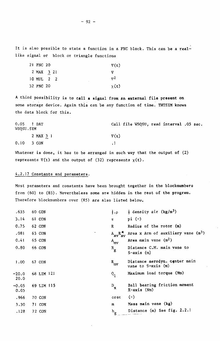
- 92 -
It is also possible to state a function in a FNC block. This can be a real
like signal or block or triangle functions
21 FNC 20 Vet) 2 MAX 3 21 V
10 MUL 2 2 v2
32 FNC 20 X (t)
A third possibility is to call a si8nal from an external file present on
some storage device. Again this can be any function of time. THTSIM knows
the data block for this.
0.05 1 DAT WSQSU.SIM
2 MAX 3
0.10 3 CON
Call file WSQSU, read interval .05 sec.
Vet)
• 1
Whatever is done, it has to be arranged in such way that the output of (2)
represents Vet) and the output of (32) represents X(t).
4.2.17 Constants and parameters.
Most parameters and constants have been brought together in the blocknumbers
from (60) to (85). Nevertheless some are hidden in the rest of the program.
Therefore blocknumbers over (85) are also listed below.
.635
3.14
0.75
.081
0.41
0.80
1.00
-20.0 20.0
-0.05 0;05
.966
3.30
.128
60 CON
61 CON
62 CON
63 CON
65 CON
66 CON
67 CON
68 LIM 121
69 LIM 115
70 CON
71 CON
72 CON
~.p
R
~ density air (kg/m3)
pi (-)
Radius of the rotor (m)
A R -= Area x Arm of auxiliary vane (m3) avav A Area main vane (m2)
mv R g
R mv
D x
cos€:
m
Distance C.M. main vane to S-axis (m)
Distance aerodyn. c4n~er main vane to S-axis (m)
Maximum load torque (Nm)
Ball bearing friction moment X-axis (Nm)
(-)
Mass main vane (kg)
Distance (m) See fig. 2.2.1
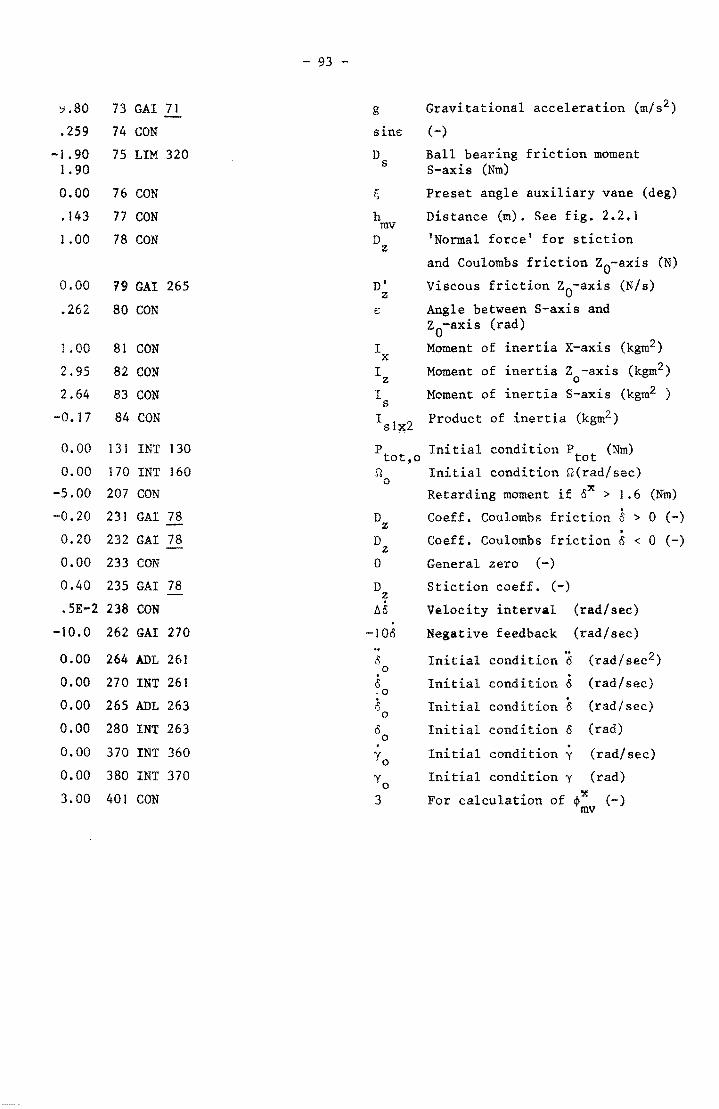
~,80
.259
-1.90 1. 90
0.00
.143
1.00
0.00
.262
1.00
2.95
2.64
-0.17
73 GAl 71
74 CON
75 LIM 320
76 CON
77 CON
78 CON
'19 GAl 265
80 CON
81 CON
82 CON
83 CON
84 CON
0.00 131 INT 130
0.00 170 INT 160
-5.00 207 CON
-0.20 231 GAl 78
0.20 232 GAl 78
0.00 233 CON
0.40 235 GAl 78
.5E-2 238 CON
-10.0 262 GAl 270
0.00 264 ADL 261
0.00 270 INT 261
0.00 265 ADL 263
0.00 280 INT 263
0.00 370 INT 360
0.00 380 INT 370
3.00 401 CON
- 93 -
g
sine
D s
~
h mv D z
D' z
I x
I z I
s I
sb!:2
Gravitational acceleration (m/s2)
(-)
Ball bearing friction moment S-axis (Nm)
Preset angle auxiliary vane (deg)
Distance (m). See fig. 2.2.1
'Normal force' for stiction
and Coulombs friction ZO-axis (N)
Viscous friction ZO-axis (N/s)
Angle between S-axis and Za-axis (rad)
Moment of inertia X-axis (kgm2 )
Moment of inertia Z-axis (kgm2 ) o
Moment of inertia S-axis (kgm2 )
Product of inertia (kgm2 )
P Initial condition Ptot (Nm) tot,o n Initial condition n(rad/sec)
o
D z D
z o
Retarding moment if OX > 1.6 (Nm)
Coeff. Coulombs friction 8 > 0 (-) . Coeff. Coulombs friction 0 < 0 (-)
General zero (-)
D Stiction coeff. (-) z
A5 Velocity interval (rad/sec)
-108 0, n
o
Negative feedback (rad/sec)
Initial condition 6 (rad/sec2) . Initial condition 0 (rad/sec) . Initial condition 0 (rad/sec)
Initial condition 0 (rad)
Initial condition y (rad/sec)
Initial condition y (rad)
For calculation of ~x (-) mv
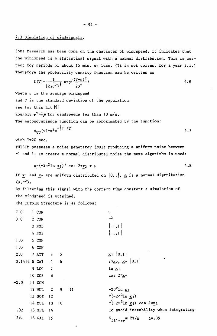
- 94 -
4.3 Simulation of windsignals.
Some research has been done on the character of windspeed. It indicates that;
the windspeed is a statistical signal with a normal distribution. This is cor
rect for periods of about 15 min. or less. (It is not correct for a year f.i.)
Therefore the probability density function can be written as
f(V)- 1 exp{(V-~)2} {21Tcr2 }! 2cr2
Whe~e ~ is the average windspeed
and cr is the standard deviation of the population
See for this Lit 191 Rou~hly v~=!p'for windspeeds les than 10 m/s.
The autocovariance function can be aproximated by the function:
~ (T)=cr2e-!-rl/T VV
with T=20 sec.
4.6
4.7
THTSlM posseses a noise generator (NOl) producing a uniform noise between
-1 and I. To create a normal distributed noise the next algorithm is used:
4.8
If !.l and ~2 are uniform distributed on ! 0,11. n is a normal distribution
(11 ,cr2 ).
By filtering this signal with the correct time constant a simulation of
the windspeed is obtained.
The THTSlM Structure is as follows:
7.0 CON 11
3.0 2 CON cr2
3 NOl I-I, I I 4 NOl ! -1,1 I
1.0 5 CON
1.0 6 CON
2.0 7 ATT 3 5 Xl 10,1 ! 3.1416 8 GAl 4 6 2~2, .!2 10,1 I
9 LOG 7 In ~.1
10 COS 8 cos 21T.!2
-2.0 11 CON
12 MUL 2 9 11 -2cr21n :1 13 SQT 12 1(-2cr2ln :1)
14 MUL 13 10 1(-2 C12ln :1) cos 271X2
.02 15 SPL 14 To avoid instability when integrating
28. 16 GAl 15 K = filter 2T16 A=.05
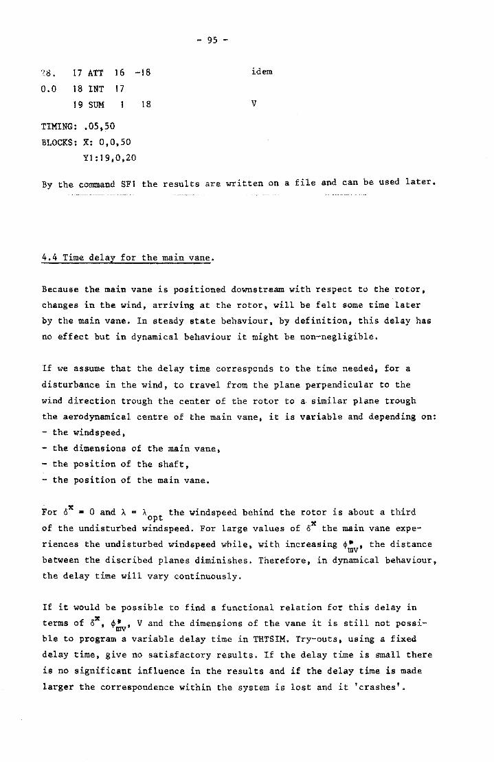
7.8, 17 ATT 16 -18
0.0 18 INT 17
19 SUM
TIMING: .05.50
BLOCKS: X: 0,0,50
Yl:19,0,20
18
- 95 -
idem
V
By the command SFt the results are written on a file and can be used later.
4.4 Time delay for the main vane.
Because the main vane is positioned downstream with respect to the rotor,
changes in the wind, arriving at the rotor, will be felt some time later
by the main vane. In steady state behaviour. by definition, this delay has
no effect but in dynamical behaviour it might be non-negligible.
If we assume that the delay time corresponds to the time needed, for a
disturbance in the wind, to travel from the plane perpendicular to the
wind direction trough the center of the rotor to a similar plane trough
the aerodynamical centre of the main vane, it is variable and depending on:
- the windspeed,
- the dimensions of the main vane,
- the position of the shaft,
- the position of the main vane.
For oX = ° and A = A the windspeed behind the rotor is about a third opt of the undisturbed windspeed. For large values of oX the main vane expe-
riences the undisturbed windspeed while. with increasing ~ •• the distance mv between the discribed planes diminishes. Therefore, in dynamical behaviour,
the delay time will vary continuously.
If it would be possible to find a functional relation for this delay in X terms of 5 , ~. , V and the dimensions of the vane it is still not possi-
mv ble to program a variable delay time in THTSIM. Try-outs, using a fixed
delay time, give no satisfactory results. If the delay time is small there
is no significant influence in the results and if the delay time is made
larger the correspondence within the system is lost and it 'crashes'.
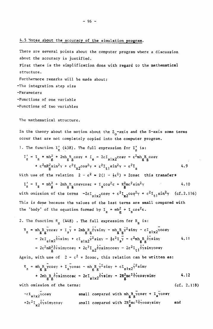
- 96 -
4.5 Notes about the accuracy of the simulation program.
There are several points about the computer program where a discussion
about the accuracy is justified.
First there is the simplification done with regard to the mathematical
structure.
Furthermore remarks will be made about:
-The integration step size
-Parameters
-Functions of one variable
-Functions of two variables
The mathematical structure.
In the theory about the motion about the Z -axis and the S-axis some terms o
occur that are not completely copied into the computer program.
1. The function It (438). The full expression for If is: z z
I' I + mh2 + Zmh R cosy + I - 2eI 1 2cosy - e2mh R cosy z z g g g s s x g g
+ e2mR2sin2y + e21 cos2y + e21 sin2y - e21 4.9 g x2 tl s
With use of the relation 2 - e2 "" 2(1 - !e2) '" Zeose: this transfer:s
I' = I + mh2 + 2mh R cosycose + I COS 28 + R2me: 2sin2y z z g g g s g
4. to
with omission of the terms -2els1x2cosy + E2Ix2CO~2y + (cf.2.116)
This is done because the values of the last terms are small compared with
the 'body' of the equation formed by I + mh2 + I cos2e:. z g s
2. The function R (448) • The full expression for R is: z z
R = mh R yeosy + I y + Zmh R cysiny - mh R y2siny - e1 1 2YCOSY z g g s g g g g s x
- ZeI 1 28ysiny + e1 1 2y2siny - !82r y - 82mh R 5ysiny 4.11 s x s x s g g
- ze:2mR~~ysinycosy + 2e:2Ix26ysinycosy - 2e2It16ysinycosy
Again, with use of 2 - 82 '" 2cose, this relation can be written as:
R z
mh R rcosy + I ycose - mh R y2siny g g s g g
+ 2mh R ~ysinycos€ - 2EI 1 25ysiny g g s x
with omission of the terms: ..
+ £Islx2y2siny
- 2R2m£2~ycosysiny g
., II •
-E:Is1x2Ycosy small compared with mh R yeosy + IsYcoSY g g
4.12
(cL 2. 118)
+2821xz6ysinycosy small compared with 2R2m82~yeosysiny and g
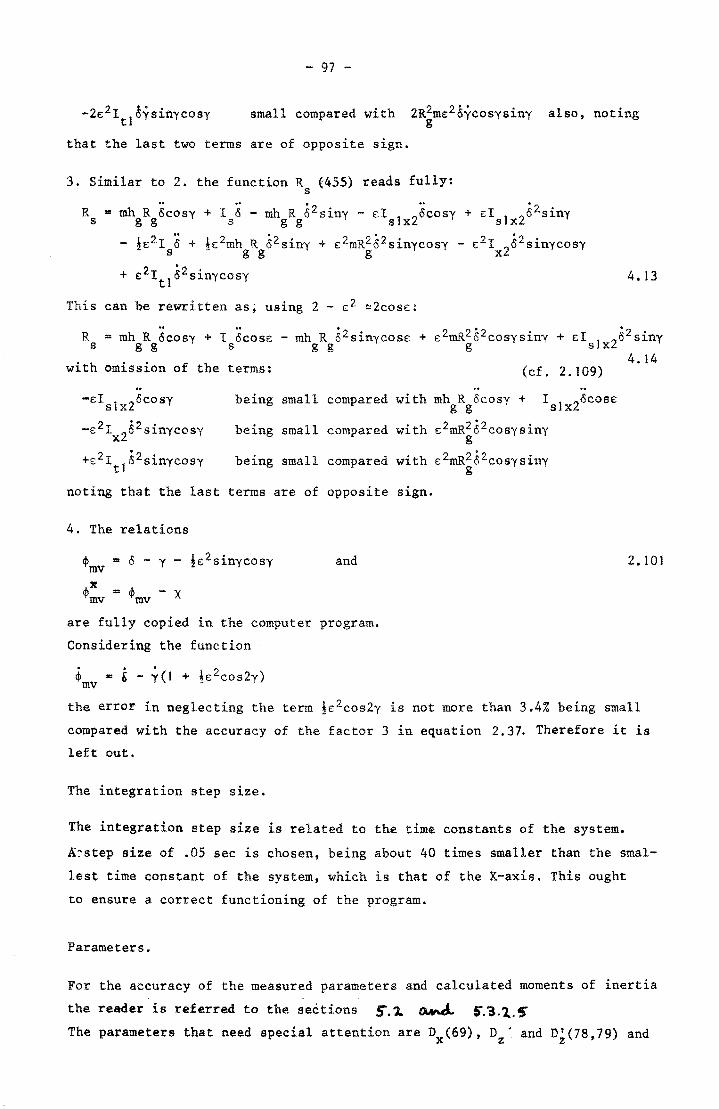
- 97 -
small compared with also, noting
that the last two terms are of opposite sign.
3. Similar to 2. the function R (455) reads fully: s ..
R = mh R ocos)' s g g
- h::LI 6 + s
+ 186 - mhgRg82Siny - eISlx25cosy + SIslx28Lsiny
!s2mh R 8Lsinv + eLmR28Lsinvcosv - s21 8Lsinycosy ~ g g , g" x2
+ e:Llt16Lsinycosy
This can be rewritten as; using 2 - SL ~2cose:
4. 13
R = mh R ~COSy + I 8cose - mh R 82sinycose + s2mRL~2cosysiny + SIslx28Lsiny s g g s g g g
with omission of the terms: (cf. 2. 109) .. ..
-sIs1x2ocosy being small compared with mh R oeos)' + Is1x2ocose: g g
-s21 62sinycosy being small compared with e2mR262cosysiny x2 g
+s2ItI82 sin)'cosy being small compared with e2mR262cosysiny g
noting that the last terms are of opposite sign.
4. The relations
~mv = 0 - y - !e2 sinycosy
x ~mv = ~mv - X
and
are fully copied 1n the computer program.
Considering the function
~ = 5 - y' (1 + ~s2cos2y) mv .
4.14
2.101
the error in neglecting the term is 2cos2Y is not more than 3.4% being small
compared with the accuracy of the factor 3 in equation 2.37. Therefore it is
left out.
The integration step size.
The integration step size is related to the time constants of the system.
~~step size of .05 sec is chosen, being about 40 times smaller than the smal
lest time constant of the system, which is that of the X-axis. This ought
to ensure a correct functioning of the program.
Parameters.
For the accuracy of the measured parameters and calculated moments of inertia
the reader is referred to the sections 5",1. ~ S.'3.l..S'
The parameters that need special attention are D (69), D ' and Dz'(78,79) and x z
- 98 -
DS (75). These friction coefficients are measured with the system at rest.
l'.:ost probably the.se. coefficients.. are not valid when the system is in motion. For Dz it ought to be 'noted that in dynamical behaviour for
ces are acting on the trunnion bearing caused by the thrust force on the
rotor, the gyroscopic moment and an unbalance of the weight of the rotor
and the main vane. How these varying forces influence the friction is not
clear. We expect that the effects are small in the scale model, but it is
clear that this is, in general, not the case for ~ull scale wi1llil.mills. If
there are forces that influence the friction about the Z -axis they can o
be taken in account via (78) which than, of course, no longer remains a
constant. That the friction terms about the zO-axis are important is il1u8-
trated in the appendix XII , showing motion under the same initial con-
ditions except for the friction about the Z-axis. . 0
Functions of one variable.
The functions of one variable occuring in the program, are the following:
Q1(f2) (121) and C (ox)(202). They are de'rived from measurements done on the av generator, see section 5.2, and on the auxiliary vane, see section 5.4.
x In fact C is not only a function of 0 , but also of A. In dynamic behaviour av therefore A-values occur that differ from the measurements. We stated the
C function separately for each configuration of t and RX • As the measu-av av
rements of C turned out to be exotic of shape and of small accuracy, the av curves are smoothed with rejection of extremities. A coorect form of the
C function is of crucial interest since often M is the major moment av av d ' . ~X ten ~ng to 1ncrease u •
Functions of two variables.
Functions of two variables (or more) form some kind of trouble in THTSIM.
The functions occuring are: CQ(A,ox),C.~(A,Qx) and C (¢x ,ox). The lacking f" mv mv
of a two dimensional interpolation function block implies that with tricks
and treats a workable version has to be made. This goes either with loss
of accuracy or with a huge set of blocks. A compromise has been made try
ing to ascertain a correct functioning in the working area.
x A satisfactory model is built for the function CQ(A,O ) giving good results
for OX smaller than 50° and acceptable results for oX > 50°.
For the yawing moment M(A,Ox) a 10% accuracy is reached within the section
1 < A < 2, but for values of A < 1 little can be said because of the lack
- 99 -
of adequate information from the measurements.
For the function C (~~ ,o~) the values are mv mv o x 0 derived for 0 ~ ~ ~ 30 only. mv
Within this section the values are within a 10% accuracy. It has to be noted
that ~~ seldom exceeds 300
mv
4.6 Some results of the computer model.
This section shows the aerodynamic functions as they operate whithin the com
puter model. It will also give some results of the c.m. that are not accounted
for in the sections that concern the comparison among wind tunnel tests and
computer results.
In the appendix XIII the graphs of CQ(A.o-), C (A,o·). C (o',~~) M mv mv
and Cav(~) as declared in the computer model are shown. They are placed
near the appendices that show the measured results to facilitate comparison.
In appendix XIV an image is shown of how the system responds if V = 0 ml sand
the main vane is given a deviation from its lowest position (y = 250 and
y = 400 resp.). The left part shows the system when all friction is omitted:
the system keeps oscillating. The right part shows the system when normal
friction is applied. To read the images the reader must realize that 0 and y
are defined in opposite direction. Therefore, by releasing the vane from a
positive angle y the shaft will move in the negative direction of o.
Finally two impressions are given for the system with two different auxiliary
vanes under a real like wind speed signal. App. XV~shows 40'seconds the angles
n ~nd, y and the angular velocity of the rotor for a winspeed about 10 m/s.
The auxiliary vane has a length of .86 m and the preset angle ~ =0°.
App XV~shows the same system but now with R· =1.06 m and ~ = -25°. The scales av are slightly different here for Q and V.
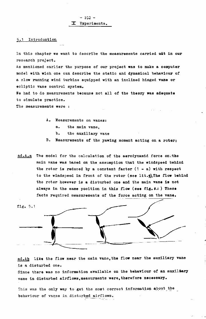
- ICC -I Experiments.
5.1 Introduction
In this chapter we want to describe the measurements carried Qat in our
research project.
As mentioned earlier the purpose of our project was to make a computer
model with wich one can describe the static and dynamical behaviour of
a slow running wind turbine equipped with an inclined hinged vane or
ecliptic vane control system.
We had to do measurements because not all of the theory was adequate
to simulate practice.
The measurements were :
A. Measurements on vanes:
a. the main vane,
b. the auxiliary vane
B. Measurements of the yawing moment acting on a roter;
ad.A.a The model for the calculation of the aerodynamid force on.:the
main vane was based on the assumption that the windspeed behind
the rotor is reduced by a constant factor (1 - a) with respect
fig. 5.1
to the windspeed in front of the rotor (see lit.~.The flow behind
the rotor however is a disturbed one and the main vane is not
always in the same position in this flow ( ••• fig. '.1 ) Thes.
facts required measurements of the force acting on the vane.
-
ad.Ab Lik. the flow near the main vane,the flow near the auxiliary vane
is a disturbed one. Since there was no information available on the behaviour of an au:xil_ary
vane in disturbed airflows,measurments were,therefore necessary.
This was the only way to get the most correct 1nformat~0~ about the
behaviour of vanes in distu~~d ai~flowso
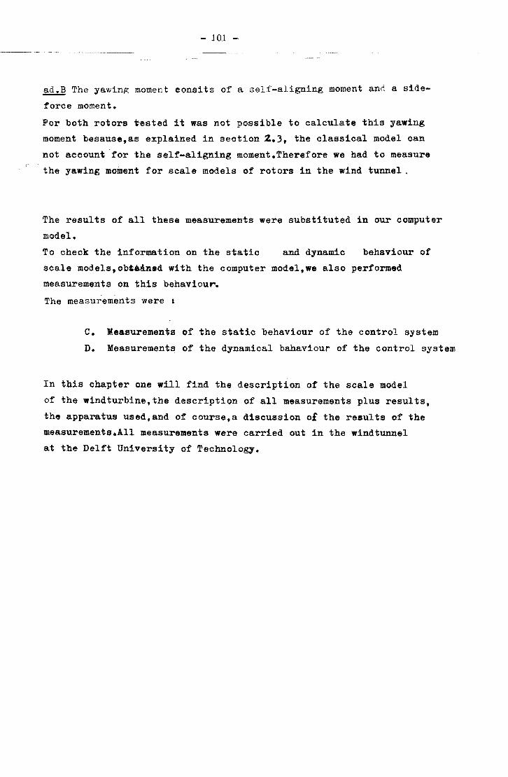
- JOJ -
ad.B The yawing moment consits of a self-aligning moment and a side
force moment.
For both rotors tested it was not possible to calculate this yawing
moment besause,as explained in section 2.3, the classical model can
not acoountfor the self-aligning moment.Therefore we had to measure
the yawing moment for scale models of rotors in the wind tunnel.
The results of all these measurements were substituted in our computer
model.
To cheek the information on the static and dynamic behaviour of
seale models,ob'&aned with the computer model,we also performed
measurements on this behaviour.
The measurements were :
c. Measurements of the static behaviour of the control system
D. Measurements of the dynamical bahaviour of the control system
In this chapter one will find the description of the scale model
of the windturbine,the description of all measurements plus results,
the apparatus used,and of course,a discussion o£ the results of the
measurements.AII measurements were carried out in the wind tunnel
at the Delft University of Technology.
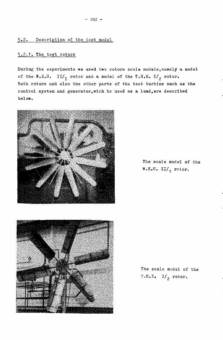
- 102 -
5.2. Description of the test model
5.2.1. The test rotors
During the experiments we used two rotors scale models,namely a model
of the W.E.U. 11/1 rotor and a model of the T.H.E. 1/2 rotor.
Both rotors and also the other parts of the test turbine such as the
control system and generator,wich is used as a load,are described
below.
The scale model of the
W.E.U. 11/1 rotor.
The scale model of the
T.H.E. 1/2 rotor.
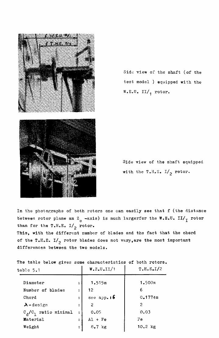
Side view of the shaft (of the
test model) equipped with the
W.E.D. II/1 rotor.
Side view of the shaft equipped
with the T.H.E. I/2 rotor.
In the photographs of both rotors one can easily see that f (the distance
b'etween rotor plane an Zo -axis) is much largerfor the W.E.D. II/I rotor
than for the T.H.E. I/2 rotor.
This, with the different number of blades and the fact that the chord
of the T.H.E. I/2 rotor blades does not vary,are the most important
differences between the two models.
The table below gives some characteristics
table 5.1
Diameter
Number of blades
Chord
A-design
Cd/C I ratio minimal
Material
Weight
W.E.TI.II/1
1.515m
12
see app. I' 2
0.05
Al + Fe
8.7 kg
of both rotors.
T.H.E.I/2
1.500m
6
0.1774m
2
0.03
Fe
10.2 kg
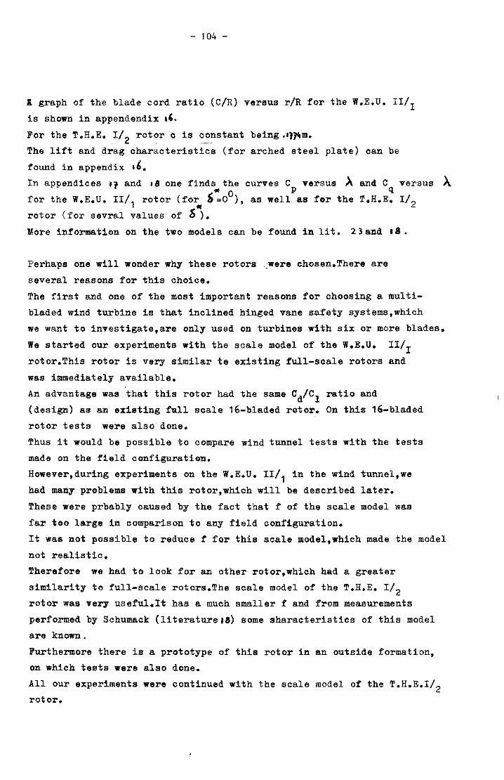
- 104 -
I graph of the blade cord ratio (c/R) versus r/R for the W.E.U. 11/1
is shown in appendendix I'. For the T .H.E. 112 rotor c is constant being "l1,m.
The lift and drag characteristics (for arched steel plate) can be
found in appendix ,6. In appendices '1 and ." one finds the curves C versus A and C versus A
* 0 p q for the W.E.U. III, rotor (fo~ S=O ), as well as for the T.H.E. 1/2
rotor (for sevral values of S). More information on the two models can be found in lit. 23 and 18.
Perhaps one will wonder why these rotors~were chosen. There are
several reasons for this choice.
The first and one of the most important reasons for choosing a multi
bladed wind turbine is that inclined hinged vane safety systems,which
we want to investigate,are only used on turbines with six or more blades.
We started our experiments with the scale model of the W.E.U. 11/1
rotor.This rotor is very similar te existing full-scale rotors and
was immediately available.
An advantage was that this rotor had the same Cd/Cl ratio and
(design) as an existing full scale 16-bladed rotor. On this 16-bladed
rotor tests were also done.
Thus it would be possible to compare wind tunnel tests with the tests
made on the field configuration.
However,during experiments on the W.E.U. 11/1 in the wind tunnel,we
had many problems with this rotor, which will be described later.
These were prbably caused by the fact that f of the scale model was
far too large in comparison to any field configuration.
It was not possible to reduoe f for this scale model,whieh made the model
not realistic.
Therefore we had to look for an other rotor,which had a greater
similarity to full-seale rotors.The seale model of the T.H.E. I/2
rotor was very useful.It has a much smaller f and from measurements
performed by Sohumack (literature,a) some sharacteristies of this model
are known.
Furthermore there is a prototype of this rotor in an outside formation,
on which tests were also done.
All our experiments were continued with the scale model of the T.H.E.I/2 rotor.
- 105 -
5.2.2. The shaft of the test model
The shaft (appendix 19 ) was mounted on the tower in such a way that
it was possible to rotate it about the tower axis.
To realize this we used a trunnion bearing. Other important requirements
were:
The main vane must be mounted on the shaft.At the same time the vane
should be able to move independently of the shaft.How this was
realized can be seen in appendix ., •
A fixed auxiliary vane must be added.
The rotation of the rotors is to be transmitted to the load (a gene
rator).In our case a pulley and V belt system was used (see photo
graph appendix 10)
The control system of our test model
During the experiments both rotors had a control system consisting
of an inclined hinged vane an. a fixed auxiliary vane.
In appendices 21 and 22 one finds the dimensions of the vane system and
its construction in the test model.
A short explanation of how this safety system works can be found in
(literature 12).
The generator.
It was not possible,for technical reasons,to use a reciprocating
waterpump (as the load of the rotor).A generator was used instead.
This,however raised a problem:a reciprocating pistonpump has a
torque which is constant approximately,while a generator has a
torque which is not constant in general.
However,the aim of our activities was to compose a dynamic model
of which the results could be compared to results of wind tunnel
experiments.
For this aim it did not matter what kind of load was used in the
dynamic model.The generator used was a Deko-Remy.a 24-voltage,
20-ampere generator.
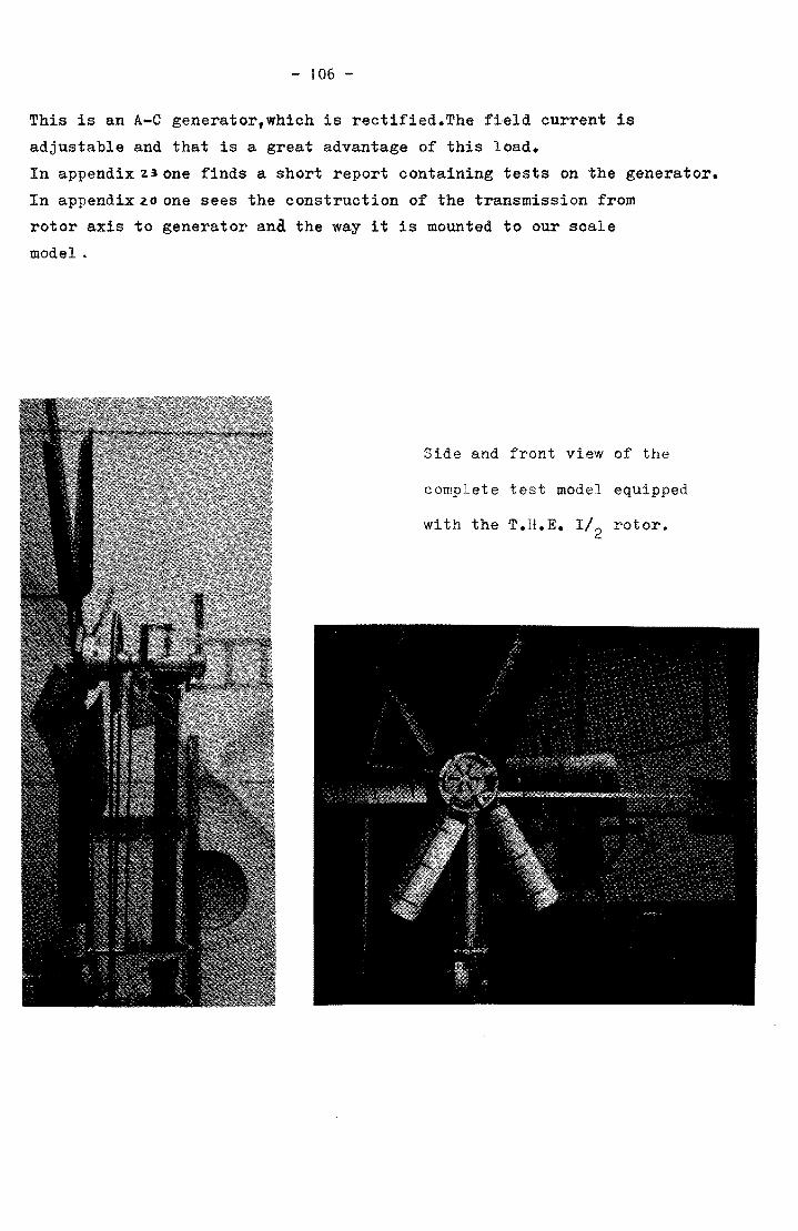
- 106 -
This is an A-C generator,which is rectified.The field current is
adjustable and that is a great advantage of this load.
In appendix ~30ne finds a short report containing tests on the generator.
In appendix 20 one sees the construction of the transmission from
rotor axis to generator ana the way it is mounted to our scale
model.
Side and front view of the
complete test model equipped
with the T.H.E. 1/2 rotor.
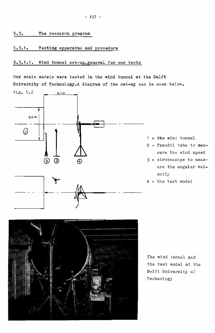
- 107 -
5.3. The research program
5.3.1. Testing apparatus and procedure
5.3.1.1. Wind tunnel set-up,general for our tests
Our scale models were tested in the wind tunnel at the Delft
University of Technology.A diagram of the set-up can be seen below.
fig. 5.2 1../ IW\
l..l. m
(j)
1 ® Q) @
',---- --
1 = the wind tunnel
2 = Prandtl tube to mea-
sure the wind speed
3 stroboscope to meas-
ure the angular vel-
ocity
4 the test model
The wind tunnel and
the test model at the
Delft University of
Technology
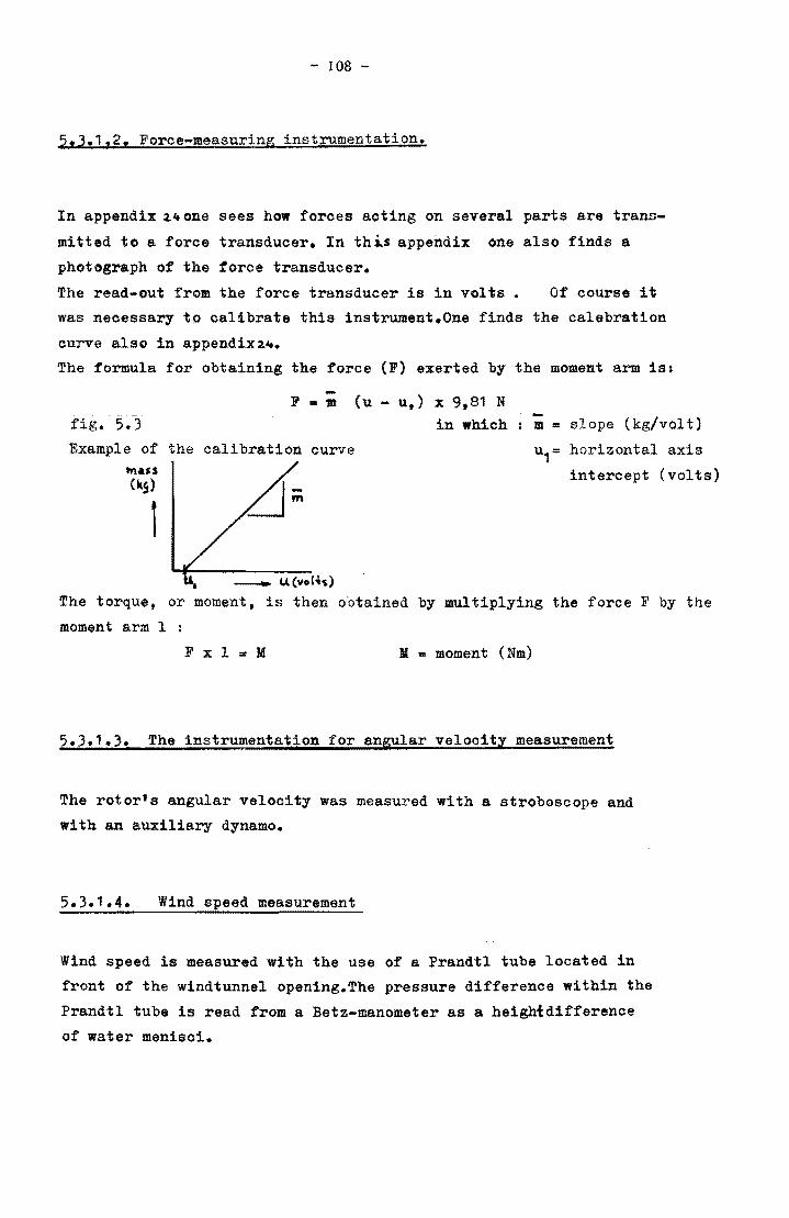
- 108 -
5,3.1,2. Force-measuring instrumentation.
In appendix ~40ne sees how forces acting on several parts are trans
mitted to a force transducer. In this appendix one also finds a
photograph of the foroe transduoer.
The read-out from the force transducer is in volts. Of course it
was necessary to calibrate this instrument.One finds the calebration
curve also in appendix~~.
The formula for obtaining the force (F) exerted by the moment arm is:
fig. 5.3 F = m (u - u,) x 9,81 N
in which
Example of the calibration curve "'&SS (kS)
t _ t.l(v.H",)
m = slope (kg/volt)
u1= horizontal axis
intercept (volts)
The torque. or moment. is then obtained by multiplying the force F by the
moment arm I
11 :: moment (Nm)
5.3.1.3. The instrumentation for angular velocity measurement
The rotor's angular velocity was measured with a stroboscope and
with an auxiliary dynamo.
Wind speed measurement
Wind speed is measured with the use of a Prandtl tube located in
front of the windtunnel opening.The pressure difference within the
Prandtl tube is read from a Betz-manometer as a height difference
of water menisci.
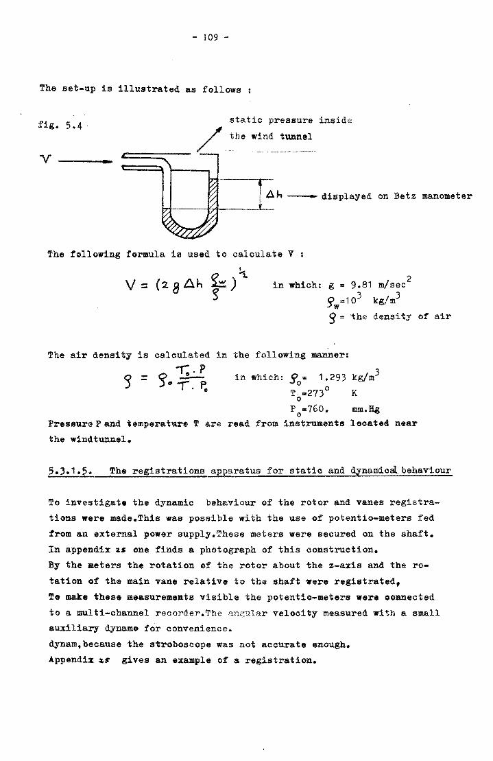
- 109 -
The set-up is illustrated as follows
static pressure inside
~ the wind tunnel fig. 5.4·
v ... c:=.=:;:---
~h • displayed on Betz manometer
The following formula is used to calculate V
~ v= (28 Ah f) in which: g :: 9.81 m/sac 2
5'w=103 kg/m3
<3:: the density of air
The air density is calculated in the following manner:
in which:
Pressure P and temperature T are read from
the wind tunnel.
5'0 = 1.293 kg/m3
T=273° K o p =760. mm.Hg o
instruments located near
The registrations apparatus for statio and dynamio&.behaviour
To investigate the dynamic behaviour of the rotor and vanes registra
tions ware made.This was possible with the use of potentia-meters fed
from an external power supply.These meters were secured on the ahaft.
In appendix 1.1 one finds a photograph of this construction.
By the meters the rotation of the rotor about the z-axis and the ro
tation of the main vane relative to the shaft were registrated,
T. make these measurements visible the potentia-meters were oonnected
to a multi-channel recorder. The anD;ular velocity measured with a small
auxiliary dynamo for convenience.
dynam,because the stroboscope was not accurate enough.
Appendi% ~s gives an example of a registration.
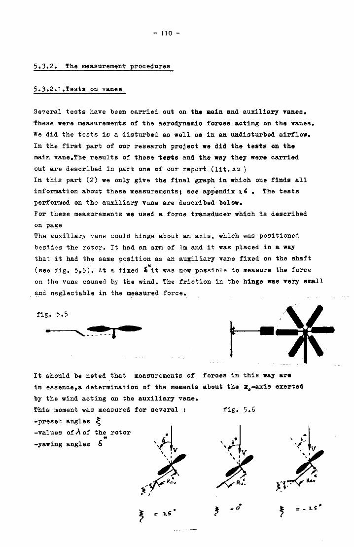
- 110 -
5.3.2. The measurement procedures
5.3.2.1.Tests on vanes
Several tests have been oarried out on the main and auxiliary vanes.
These were measurements of the aerodynamic foroes acting on the vanes.
We did the tests is a disturbed as well as in an undisturbed airflow.
In the first part of our research projeot we did the tests on the
main vane.The results of these ~e8.s and the way they were carried
out are desoribed in part one of our report (lit.~2)
In this part (2) we only give the final graph in whioh one finds all
information about these measurements I see app'endix :2.'. The tests
performed on the auxiliary vane are described below.
For these measurements we used a foroe transducer which is described
on page
The auxiliary vane could hinge about an axis, whioh was positioned
besides the rotor. It had an arm of 1m and it was placed in a way
that it had the same position as an auxiliary vane fixed on the shaft .. (see fig. 5,5). At a fixed' it was now possible to measure the foroe
on the vane caused by the wind. The friotion in the hinge was very small
and neglectable in the measured force.
fig. 5.5
"·--'·--~--I •
It should be noted that measurements of forces in this way are
in essenoe,a determination of the moments about the E.-axis exerte4
by the wind acting on the auxiliary vane.
This moment was measured for several fig. 5.6 -preset angles ~ -values ofAo! the rotor
'i~ ,,~ , ·1 " -yawing angles b
1 ;t j{ " I
- ~.~ " ,I
rl·· ~: R<l~ )/ ,
• , = _ l.S·
~ • , ::0
;: l.S
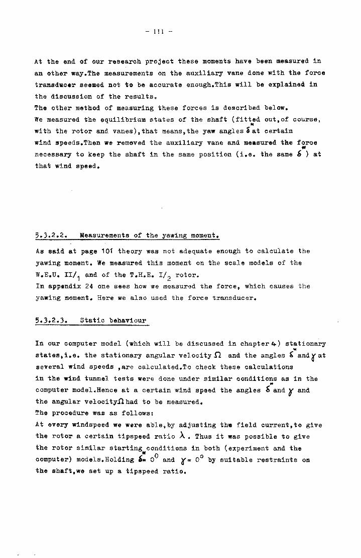
- III -
At the end of our research project these moments have been measured in
an other way.The measurements on the auxiliary vane done with the force
transd.oer se •• ed not to be acourate enough.This will be explained in
the discussion of the results.
The other method of measuring these forces is described below.
We measured the equilibrium states of the shaft (fitted outtof course, II
wi th the rotor and vanes) t that means, the yaw angles' at oertain
wind speeds.Then we removed the auxiliary vane and measured the foroe .. necessary to keep the shaft in the same position (i.e. the same ~ ) at
that wind speed.
Measurements of the yawing moment.
As said at page 101 theory was not adequate enough to calculate the
yawing moment. We measured this moment on the scale models of the
W.E.U. 11/1 and of the T.R.E. 1/2 rotor.
In appendix 24 one sees how we measured the force, which causes the
yawing moment. Here we also used the force transducer.
Static behaviour
In our computer model (which will be discussed in chapter 4) stationary w
states. i.e. the stationary angular velooity n and the angles' andr at
seYeral wind speeds tare calculated.To check these calculations
in the wind tunnel tests were done under similar conditions as in the .. computer model.Hence at a certain wind speed the angles , and 0 and
the angular velocityJlhad to be measured.
The procedure was as follows:
At every windspeed we were able,by adjusting th. field current,to give
the rotor a certain tipspeed ratio A. Thus it was possible to give
the rotor similar starting conditions in both (experiment and the
oomputer) models. Holding ,: 0° and r= 0° by suitable restraints on
the shaft,we set up a tipspeed ratio.
- 112 -
After that we removed the restraints on the shaft,so that it was ,. possible for b, '( and A to as~ume the stationary values.It was
simple to measure the angles ~ and r by using the potentio-meters.
Pictures of these meters and their cha racteristics can be seen
in appendix U ,as said o. page log.
5.3.2.4. Dynamic behaviour.
As said in the discussion of the apparatus used in section' .....
registrations of the dynamio behaviour of the rotor and vanes have
been made.In studing this behaviour we used two methods: 4t
The first: In a stationary' state (i.e. with constant ~,~ and ).. ) .. 0
we gave the shaft a deviation ( ~ ~ ) of about 30 • Then we let
go the shaft and registrated at the multi-channel recorder the 'It
changes ef ~, '1 and the angular velaei ty (Jl).
The second: inoreasing the windspeed from 0 to 14 m/seo with starting .. conditions v -0 m/sec, ,. 0°, r- 0° and, self-evi~ently, A. i. Hence it was possible to make a registration of b, yand the
angular Yeloeity course.
With these registrations it was very easy to find the wind speed at
which oscillations of the shaft with rotor and vanes occured.
These registrations were made by using the same potentia-meters,
as during the measuremants of the stationary states. in combination
with the multi-channel recorder.
Moments of inertia.
+ To describe the dynamic behaviour of the rotor vanes (of the oomplete
scale model) in our oomputer model we had to know the moments of
inertia of all the parts the soale model conmi.ts of.!h ••••• ments
were all measured by the physioal pendulum method. In appendix 27 one
finds all the results of the calculations of the moments of inertia
of all parts of the scale model.
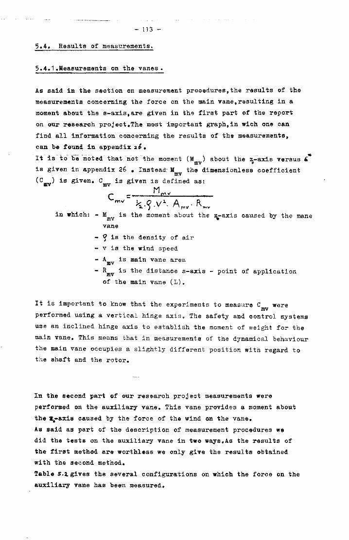
- 113 -
5.4. Results of measurements.
5.4.1.Measurements on the vanes.
As said in the seotion on measurement prooedures,the results of the
measurements concerning the force on the main vane,resulting in a
moment about the a-axis,are given in the first part of the report
on our reaearch project.The most important graph,in wioh one can
find all information oonoerning the results of the measurements,
can be found in appendix 2&.
It is to b-e-noted that not the ... moment (M ) about the z-axis versus , mv 0
is given in appendix 26 • Instead.]( the dimensionless coefficient mv
(Cmv) is given. C is given is defined as: mv M emil ::: -, -o-v",,;;,;,v;""-A---O--
.:s... ). . ~v' f\""v
in which: - Mmv is the moment about the ir&xis caused by the mane
vane
- ~ is the density of air
- v is the wind speed
- A is main vane area mv - R is the distance s-axis - point of application mv
of the main vane (L).
It is important to know that the experiments to measure C were mv
performed using a vertical hinge axis. The safety and oontrol systems
use an inclined hinge axis to establish the moment of weight for the
main vane. This means that in measurements of the dynamical behaviour
the main vane occupies a slightly different position with regard to
the shaft and the rotor.
In the second part Qf our researoh project measurements were
performed on the auxiliary vane. This vane provides a moment about
the Z.axis caused by the force of the wind on the vane.
As said as part of the description of measurement procedures we
did the tests on the auxiliary vane in two ways.As the results of
the first method are worthless we only give the results obtained
with the second method.
Tabl. S.~gives the several configurations on which the force on the
auxiliary vane has been measured.
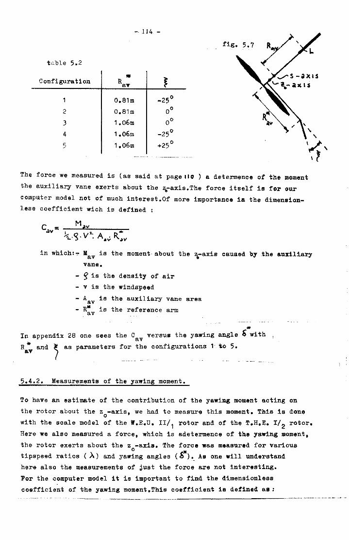
table 5.2
II Configuration R aT
1 0.81m
2 0.81m
.3 1.06m
4 1.06m
5 1.06m
-- 114 -
J _
250
00
0 0
_2,0
+25 0
" .. -~---.----
fig. 5.7
, , ,
'1' The force we measured is (as said at pagetlO ) a determence of the moment
the auxiliary vane exerts about the ~-axis.The force itself is for our
computer model not of much interest.Of more importance ia the dimensionless coefficient wich is defined :
C:. M;'II av I 2. D-
~ ,0. V . A . ~ - :') .IV ~'II
in which:~ Mav is the moment about the \-axis caused by the auxiliary vane.
- s> is the density of air
- v is the windspeed
- A is the auxiliary vane area av - Rit
av is the reference arm
... In appendix 28 one sees the Cav versua the yawing angle ~ with
R it and ~ as parameters for the configurations 1. too 5. aT I
5.4.2. Measurements of the yawing moment.
To have an estimate of the contribution of the yawing moment acting on
the rotor about the z -axis, we had to measure this moment. This is done o with the scale model of the W.E.U. II/1 rotor and of the T.H.E. 1/2 rotor.
Here We also measured a force, which is adetermence of the yawing moment,
the rotor exerts about the z -axis. The force was measured for various o " tipspeed ratios (A) and yawing angles (S ). As one will understand
here also the measurements of just the force are not interesting.
For the computer model it is important to find the dimensionless
coefficient of the yawing moment.This coefficient is define4 a8 :
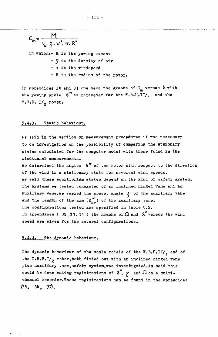
- 115 -
M eM = 1 '-":a..g.V:..,,-.R:
in which:- M is the yawing moment
- 9 is the density of air
- T is the windspeed
- R is the radiuB of the rotor.
In appendices 30 and 31 one sees the graphs of C versus X with m the y~wing angle SM as parameter for the W.E.U.II/
1 and the
T.H.E. 1/2 rotor.
Static behaviour.
As said in the section on measurement procedures it was necessary
to do investgation on the possibility of comparing the st~onar,y
states calculated for the oomputer model with these found in the
wind tunnel measurements.
We determined the angles £* of the rotor with respect to the direction
of the wind in a stationary state for severeal wind speeds.
As said these equilibrium states depend on the kind of safety system.
The systems we tested oonsisted of an inclined hinged vane and an
auxiliar,y vane.We varied the preset angle ; of the auxiliary vane
*' and the length of the arm (R ) of the auxiliary vane. av The configurations tested are specified in table 5.2.
In appendioes ( 32 ~.33. 34 ) the graphs of!l and S* versus the wind
speed are given for the several configurations.
The dynamic behaviour.
The dynamic behaviour of the scale models of the W.E.U.II/1 and of
the T.H.E.I/2 rotor,both fitted out with an inclined hinged vane
plus auxiliary vane,safety system,was investigated.As said this
could be done making registrations of ~Wf 'If and n on a mul ti
channel recorder. These registrations can be found in the appendices
(35" 36, 37) •
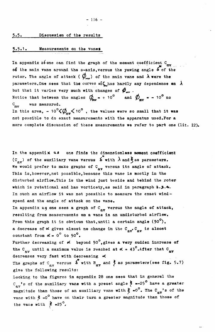
- 116 -
5.5. Discussion of the results
Measurements on the van ••
In appendix ~'one can find the graph of the moment coefficient C • mv
of the main vane around the a-axis,versus the yawing angle' of the
rotor. The angle of attack ( ~M~) of the main vane and A were the
parameters. One sees that the curves o£~has hardly any dependenoe en A but that it varies very much with ~hanges of ;1IIV . Notice that between the angles ¢mv" + 1 0° and ¢mv GO - 10
0 no
Cmv was measured.
In this area, - 100 <¢mT< 100
, the values were so small that it was
not possible to do exact measurements with the apparatus used.For a
more complete discussion of these measurements we refer to part one (lit. 22).
In the appendi)( 2.' one finds the dimensionless moment coefficient It
(Cav) of the auxiliary vane versus ~ with ~ and~as parameters.
We would prefer to make graphs of C versus its angle of attaok. av This is,however,not possible,besause this vane is mostly in the
disturbed airflow.This is the wind just beside and behind the rotor
which is rotational and has vorticety,as said in paragraph a.,.+. In such an airflow it was not possible to measure the exaot wind
speed and the angle of attack on the vane.
In appendix 4Q one sees a graph of C versus the angle of attack, ;;1 av
resulting from measerementa on a vane in an undisturbed airflow.
From this graph it is obvious that,until a certain angle (500 )t
a decrease of« gives almost no change in the C.C is almost av av oonstant from ~- 0° to 500
•
o Further decreasing of oC beyond 50 ,gives a very sudden inorease of
the Cav until a maximum value is reached at ~ = 43°.After that Cav decreases very fast with decreasing <
1t The graphs of C versus ~ with R and ~ as parameter. (see fig. 5.7) av av ( give the following results:
Looking to the figures in appendix 28 one sees that in general the
C 's of the auxiliary vane with a preset angle l _-25° have a greater av ( magnitude than those of an auxiliary vane with ~ =0°. The Cav's of the
vane with ~ _0° have on their turn a greater magnitude than those of
the vane wi th ~ _25°,
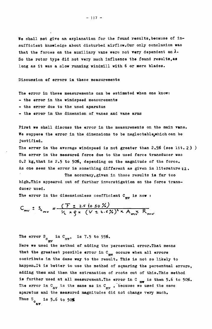
- 117 -
We shall not give an explanation for the found results,because of in
sufficient knowledge about dist~rbed airflow.Our only conclusion was
that the forces on the auxiliary vane were not very dependent onA.
So the rotor type did not very muoh influenoe the found results.a.
long as it was a slow running windmill with 6 or more blades.
Discussion of errors in these measurements
The error in these measurements can be estimated when one know:
- the error in the windspeed measurements
- the error due to the used aparatus
- the error in the dimension of vanes and vane arms
First we shall discuss the error in the measurements on the main vane.
We suppose the error in the dimensions to be neglectabl~whichcan be
justified.
The error in the average windspeed is not greater than 2.5% (see lit. 23 )
The error in the measured force due to the used force transducer was
0.2 kg,that is 2.5 to 50%, depending on the magnitude of the force.
As one sees the error is something different as given in literaturea~.
The accuraoy,given in those results is far too
high. This appeared out of further inverstigation on the force trans
ducer used.
The error in the dimensionless coefficient C is now : mv
The error S in C • is 7.5 to 55%. Cmv mv
Here we used the method of adding the percentual error. That means
that the greatest possible error in C occurs when all errors mv contribute in the dame way to the result. This is not so likely to
happen.It is better to use the method of squaring the peroentual errors,
adding them and then the extranation of roots out of this.This method
is further used at all measurement.The error in C is then 5.6 to 50%. mw
The error in Cav is the same as in Cmv • because we used the same
aparatu8 and the measured magnitudes did not change very much.
Thus S is 5.6 to 5~ c aT.
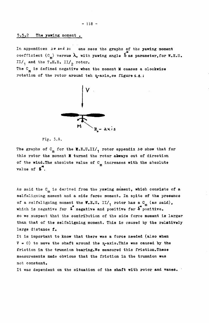
- 118 -
The yawing moment •
In appendices 30 a.nd 31 one sees the
coefficient (C ) versus A, with yawing m III, and the T.H.E. 1I/2 rotor.
graphs of the yawing moment .. angle S as parameter,for W.E.U.
The Cm is defined negative when the moment M ouases a olockwise
rotation of the rotor around tah ~-axis.se figure S.8.:
ax., s
Fig. S.B.
The graphs of Cm for the W.E.U.II/1
rotor appendix 30 show that for
this rotor the moment M turned the rotor aeways out of direction
of the wind.~he absolute value of C increases with the absolute .. value of , •
m
As said the C is derived from the yawing moment, whioh consists of a m
selfaligning moment and a side foroe moment. In spite of the presence
of a selfaligning moment the I'.E.U. 11/1 rotor has a C (as said), ~ * m
which is negative for ~ negative and positive for ~ positive.
so we suspect that the contribution of the side force moment is larger
than that of the selfaligning moment. This is caused by the relatively
large distanoe f.
It is important to know that there was a foroe needed (also when
V = 0) to move the shaft around the ~-axis.This was caused by the
friction in the trunnion bearing.We measured this friction. These
measurements made obvious that the friction in the trunnion was
not constant.
It was dependent on the situation of the shaft with rotor and vanes •.
- 119 -
HVTvever, the oontribution of this to the measured yawing moment was small.
As full-soale models in the field (in the normal situation) have a com-
parable yawing force ratio,this is not taken in
In appendices ~. one sees the graphs of Om measured on the T.H.E. 1/2
rotor. These are a little different from those obtained with the W.E.U • ... 11/1 rotor. The Cm changes (for almost all ~ ) with.Afrom positive to
negative or in the opposite way.At the T.H.E.I/2 rotor the selfaligning
moment had e big contribution to the yawing moment,which depends on
" a and X. This resal ted in a yawing moment that was for a certain value
of S·positive as well as negative depending on A.The most important
reason of this behaviour was the smaller f ,whioh was now oomparable
to that for full-soale models.Also during these measurements friotion
in the trunnion bearing has been measured.This was also here not con-.. stant and ohanged very muoh with changing S.
The average moment needed to overcome this friction was 0.525 Nm.
This was measured at a distance Rri0-]M from the z.-axis.When the yawing
moment is small,which often occured at the T.H.E. 1/2 rotor,the friction
will affect the measurements.The apparatus (the force transducer) we
used was not accurate enough for low values of the yawing moment.For
small values of Cm the rotor fluttered around the ~-axistwhich caused
relative changes in the foroe we wanted to measure. The results found
near the ~axis are therefore not reliable.
We drew the graphs of C versus A using the points with C ~ 0.0 1 only. m III m'
The grphs show that only C versus A with ,. 200 intersects the m
other graphs and d.es not vary much with the changing o£ X. ~.. 0
At •• ! 10 the yawing moment could not be measured,for the earlier mentioned reason.
Disoussion of errors in C m
The error in the yawing moment consists of:
- the error in the windspeedmeasurements
- the error caused by the used apparatus
- the negleotable error in dimensions of the system
The error in the windspeed is of course still about 2.5%oAlso at these
measurement~we had an error oaused by the used apparatus (the foroe
transducer).This was the error in the measured force,which determined
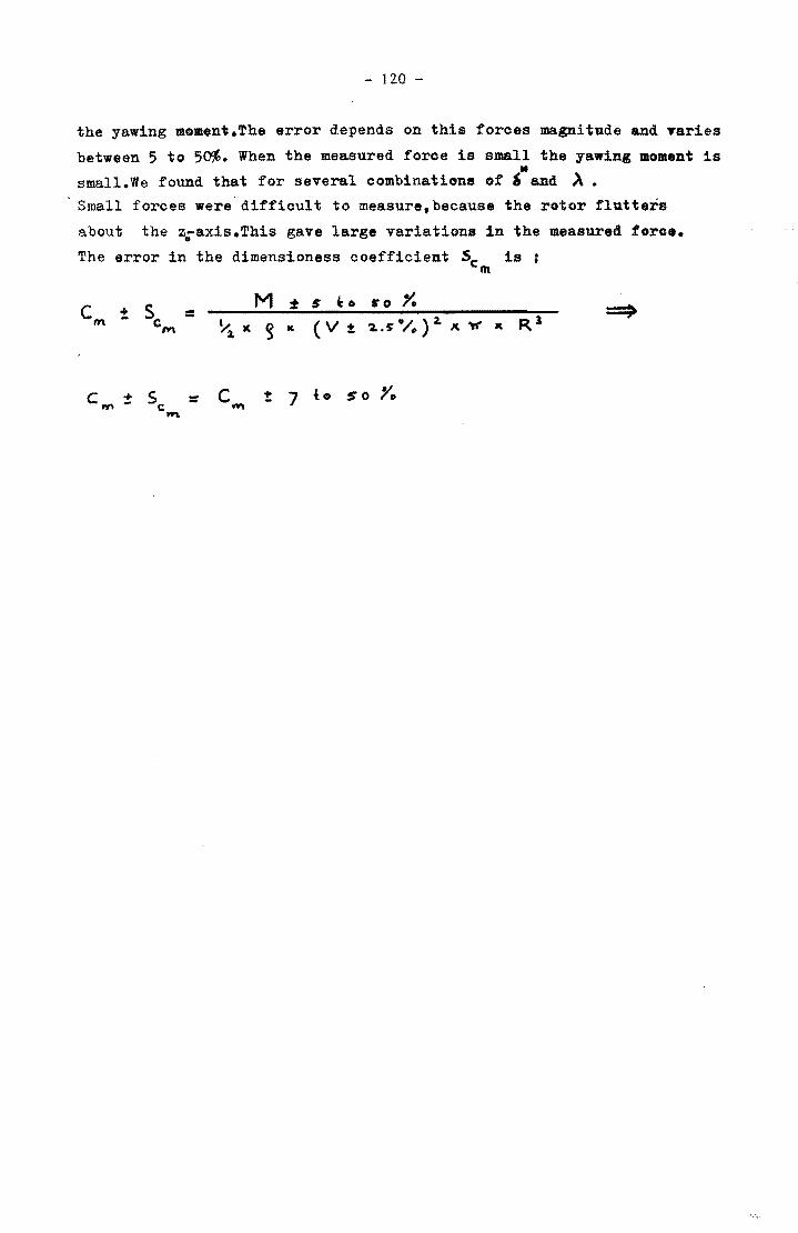
- 120 -
the yawing moment.The error depends on this forces magnitude and varies
between 5 to 50%0 When the measured force is small the yawing moment is If
small.We found that for several combinations of , and ~.
, Small forces were" difficul t to measure, because the rotor flutters
about the z:axis.This gave large variations in the measured force.
The error in the dimensioness ooefficient Sc is; m
eM ~ Sc M :t S ~. so Y. = '1.S' -/ .. ) 2- R,3 % K ~ ac; (V t x.'W' K M ~
eM ± Sc - C t 7 to so Yo - ~ ......
-121 . .-
5.5 • .3 The stationary behaviour
In the appendices .32,130,34 the graphs of the stationary behaviour of the T.H.E.I/2 rotor are given.There are no graphs of the stationary
behaviour of the •• E.U. III, rotor because this rotor was ver.y unstableo
There were no stationary stated to be found.Only some measurements of
the dynamical behaviour were done,which are described in &.~4.
Configuration' (appendix 31)
The T.H.E. 1/2 equipped with this safety system,demonstrates clearly
that with this system the angular speed could be limited.lncreasing
the windspeedngave in first instance an increasing of the angular 4rf
speed (n) and the angle of yaw ( h ).
fl,however,increased with V until a maximum was reached after which
it started to deorease. N
The increase of ~ wi th V depends on the point at which the equili-
brium of the moments around the ~-axis is reached.
The parameters such as dimension of vanes and vane arms,the preset
angles,the load and rotor type determine these moments.
The moment about the ~-axis out of the direetion of the wind is
almost entirely due to the force on the auxiliary vane.This is shawn
in table 5.3 in appendix 34.a .In this appendix one finds the moment about
the ?-axis caused by the auxiliary vane(M ) and the contribution ,. av of the yawing moment (M) about this axis.
Theae relllults are obtained by using the measurements on stationary
behaviour,the 0 av of the used auxiliary vane and the C m of the
T.H.E. I/2 rotor. More information on the moments about the ~-axis can be obtained
when mo •• measurements on the stationary behaviour of the main vane
are done.ln the measurements of stationary behaviour the angle of
yaw of the main vane was not measured.
When one wants to calculate the moment the main vane produces Mmv
about the z.axis one has to know this angle.The M varies namely mv . with the angle of yaw and also with ~. This is shown in appendix 26,
in which one finds the eoefficient(O )of the- yawing moment versus &'! mv The moment M must aqual the moments M and M.
mv u * As said configuration 1 showed an increase of S with increasing V • .. It is obvious that Sand 11 are very much conneeted,wich is shown
in appendix ll.AIl moments involved are funotions of ~, R:v and V.
- 122 -
Configuration 2 (Appendix 32)
This one is almost
preset angle ~ of
This resulted in a
the same as configuration 1 but o the auxilary vane from - 25 to
tf not so fast increase of S with
that we ohanged the
00
•
increasing winds peed
which, of course,caused a higher angular velocity (11). With this configuration!t was not clearly bounded.It is a pity that
we do not know the stationary of this configuration at windspeeds
higher than 12m/seo. This was caused by the fact in the windtunnel
it was possible to produce a windspeed greater than 14m/sec.
Configuration:3 (Appendix 33)
This one is different from 2 only in that we made the arm of the
auxiliary vane nonger (1.06 m instead of 0.81 m).The aspect of the
graphs is almost the same as those obtained at configuration 2. 11ft
The only difference is that g reached is higher and 11 is some-
thing smaller than at 2. Also here !l was not clearly bounded.
Configuration 4 (Appendix 33)
This one is the same as :3 only the preset angle was changed from o 0 o to-25. The aspect of the graphs of 1 and 4 is almost the same • ..
The difference is the fact that in 4 a increased faster with increa-
sing windspeed,which was, of course by the longer arm of the
auxiliary vane.Further it will be clear that the maximum value of 11 is smaller and found at a lower windspeed.Also the decrease of!l
beyond the maximum,wi~h further increase of V,was faster.
Confuguration 5 (Appendix 34)
.. Is as 4 only now the preset angle as + 25°.This resulted in & hardly
increasing with increasing windspeed.
That caused a steady increase of 11 • Thus this system did not limitfl
at all in the important range windspeeds,namely till 12m/sec.
It is to be noted that the stationary states will change when a
preset angle of the main vane is introduced. During these e2periments
the main vane had ( for teohnioal reasons ) no preset angle. Giving the
main vane a preset angle only the equilibrium states will change.
The aerodynamic behaviour, however remains the same. So it possible
to introduce this in the computer model without further complications.
~ J23 -
Discussion of errors in these measurements
The error in the stationary behaviour consists of
an error in the average windspeed of 2.5%
an error in the yawing angle '·of ,0 an error in the angular velocity (n) of.5 to 1 rad/sec.
The error in!l is due to the read off accurancy of the stroboscope
and (eTen more) the point at which one finds the frequenoy of the
rotor in conformity with the frequency of the stroboscope.At a
low angular velocity (!l) this gave an error of about 0.5 rad/sec.
which increases with increaslng!lto about' rad/sec. The error in
the measurements of 11 using the auxiliary dynamo is the same.
The auxiliary dynamo has been calibrated with the strobosoope.
5.5.4. The dynamioal behaviour
In appendiceli!US'-irone sees some examples of registrations of dynamical
behaviour made with a multi-channel recorder.They were done On the
W.E.U. II/1 rotor and the T.H.E.I/2 rotor.The examples 1 and 2
ooncern measurements on the W.E.U.II/1 rotor.From these it is obvious
that the behaviour of the W.E.U.II/1 rotor is not stable.lt was almost
impossible to find some stationary states.Giving the shaft with rotor tt 0
ancl vanes a displacement of ~ of about 30 resulted in large oscillations
as one can see in the registrations.
As already said the W.E.U.II/, rotor was unstable.This was due to a
large f, in comparison with full-scale models and the T.H.E.I/2 rotor.
The large f gave such a great side force moment,that the contribution
of this moment to the yawing moment was large compared to that of the
selfaligning moment.
The examples" -, concern the dynamical behaviour of the T.H.E. I/2 rotor. These -~exampfes concerIi~ the registra.tIon~s-o~f the-be-lla.-no·ur
of the rotor and vanes when they are unchained, after having had
a giving aside from the equilibrium state (see also appendices 36 and 37).
3 The model (according to configuration 2) got at a windspeed
of .,m/sec. a turn aside out of the equilibrium state of +A ~ • + 30· after which the system was unchained. One sees the
shaft is moving through the equilibrium state after wioh in
about 20 sec. the old equilibrium state is reached.
- 124 -
i The model under the same conditions as 1,but at windspeed of
10m/sec. The turn aside was + 270 out the equilibrium state
• 0 of '=57 .After unchaining it is to be denoted that the shaft
is moving with a greater speed through the equilibrium state.
It moves on to a yawing angle of 10°, after which the old
equilibrium state of S·: 57° is reached in about 30 sec.
i The model under the same concitions and at the same windspeed
of 10 m/sec.
The turn aside out of the equilibrium state is now in the
opposite way namely from S*= 57° to ~. 0°. After un
chaining the shaft moves through the equilibrium state and
reaches this state after about 100 sec.
6 The model according to configuration 3 got at windspeed of
fro/sec. a turn aside out of the equilibrium state of ~S. + 30°.
after unchaining one sees that also here the rotor moves through
its old equilibrium state.This one is reached after 10 sec.
Some more examples of dynamical behaviour are given.Allother (Apr'~7)
examples give the same view as described above.
There were no registrations made of ~and r at increasing the wind speed * 0 from 0 to 14 mlsec. with starting conditions V = 0 m/sec. ,6 = 0 ,
o r = 0 and, self-evidently, A = O. It had no sense to do that, because
the time necessary to increase the wind speed frem 0 to 14 mls.c. was
very long.
- 125 -
5.6. Results of the computer model.
5.6.1.The static behaviour calculated with the computer model.
For the oalculaUon of the~ static behavfour with the oomputer model
results of measurements were used.
The results used were:
! The yawing moment coeffiecient _2 The coeffioient C of the main Vane mv 1 The coefficient C of the auxiliary vane av
To use the results of 2 and 3 some oorreotions had te be made.
The dimensionless force coeffioient of the main vane baa to be
corrected fo~ its own speed.This correction was only neoessary
for the calculation of the dynamical behaviour.
The correotien factor was: 3 ¢.nv- A._v see. § 2..3.3. V
In the results of the measurements of the dimensionless force .. coefficient C (of the auxiliary vane) as funotion of ~ with av Ra~ and ~ as parameters were exotic of shape. See also the dis-
cussion of results of measurements.
Therefore the curves were smoothed under rejection of extremitieso
They can be found in appendices ~.
Using 1,2 and 3 in our oomputer model,gave results for the statio
behaviour which can be found in appendiees32-3~The static behaviour
acoording to caloulation with our computer model are the dotted
lines in these graphs.One sees that the oonformity between experiment
and oomputer model is reasonably good in the graphs '.2,3 and 50 !II
There were ~,~ {is , calculated in the computer model)deviates ... from , ( is b measured ) one sees a corresponding deviatiQll in
the opposite way in n . These deviations however lie in the
spreading of the measured as well as the caloulated results.
In 4 computer model and experiment are not very conform. Until V -'II
6 m/sec. both are quitte equal but for V )6m/seo. ~ increase more eM
with increasing V than ~ with the corresponding consequences for
11 in the opposite way. There is no waterproof explanattion for
this disorepance.
- 126 -
5.6,2. The dynamic behaviour oalculated with the computer model.
The dynamical behaviour of the T.H.E. I/2rotor,as measured,was simu
lated with the computer model.The conditions,such as the several
configurations of the scale model and the starting conditions,were
the same as during the measurements.Using the results of measurements
it was possible to check the accuracy of the computer model.
In appendix 38-41 0ne finds some results of measurements and corres
ponding (for what means the configuration and starting condition)
calculations of the dynamical behaviour.
The figures are results got with configuration 2,3 and 4, whioh
were tested at several winfspeeds.One sees that for these confi
gurations experiment and computer model do reasonable agree.
The difference between experiment and computer model is mainly
due to the behaviour of the main vane. The dynamical behaviour of
this vane in the computer model does not agree with the experiment.
From the registrations 4,' J 8 of r this is clear. There can be several
reasons for these differences :
- C~v was only measured in stationary states.Furthermore
the measurements were performed for a limited number of
parameter combinations.
Nevertheless these measurements were used to calculate the
dynamical behaviour.Calculation of C for an unknown value mv of ¢MV and A is therefore not very accurate.
-The correction for the vane's own motion is a poor approxi
mation of reality.One understands that when only the stationary
behaviour of the main vane is measured one will not know the influence of the vane's dynamical motion on the dynamical
behaviour of the shaft.
-Furthermore there were no measurements done on the influence
of the vane arm length R and preset angle ~ ,of the auxiliary av 5 vane,on the dynamical behaviour of the main vane.Looking to
the results one sees that ~ has for each configuration an
other value.More investigation should be necessary •.
-An other problem is that the computer model does not use a time
delay.This means that in the computer model the force on the
main vane is calculated with the windspeed felt by the rotor
on that moment.In practice the main vane will feel this wind
speed just after i to 1 second.The air needs time to pass the
rotor and to reach the main vane.See also ~ 4.4.
To create a correct model this effect should be introduced.
- 127 -
The last problem we met was that the dimensions of the a,irflow
were for some experiments to small.We had some oonfigurations
with which the main vane entered the boundary of the airflow -. when we unchained the rotor at 6 = 0 at a windspeed of 10 m/sec.
In the marginal area of the a,irflow the windspeed is mostly not
the same as in the centre of the wind airflow.Hence the force
on the main vane will change by entering this area, The experiments
whioh the main vane enters this area are therfore rejected.
Furthermore it has to be noted that investigation on the airflow
(windprofile) (see lit. 2' ) shows that also in the oentre the
windspeed is diffioult to fix exact.This also will give small
differences between oomputer model and experiment.
Conoluding one oan say that oomputer model and experiment do reasonable
agree with each other .Nevertheless it deserves a reoommendation to
optimalize the computer model, for with respeot to the problem of the
time delay and to do some more investifations on the behaviour of the
main vane,specially the dynamical behaviour.It has to be noted that the
error in measurements of C is very large specially for small values av is
of Cav • In the graphs the error indicated.One can understand (looking to
apr :nII:+2.8 ) that according to the magnitude of the error it is wrong <III:
to conclude that the ourves show the real oourse of C versus b. av
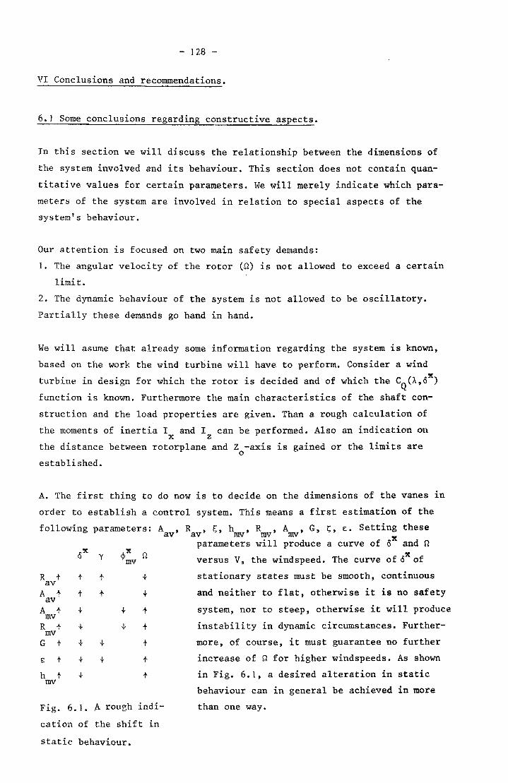
- 128 -
VI Conclusions and recommendations.
6.1 Some conclusions regarding constructive aspects.
In this section we will discuss the relationship between the dimensions of
the system involved and its behaviour. This section does not contain quan
titative values for certain parameters. We will merely indicate which para
meters of the system are involved in relation to special aspects of the
system's behaviour.
Our attention is focused on two main safety demands:
1. The angular velocity of the rotor (n) is not allowed to exceed a certain
limit.
2. The dynamic behaviour of the system is not allowed to be oscillatory.
Partially these demands go hand in hand.
We will asume that already some information regarding the system is known,
based on the work the wind turbine will have to perform. Consider a wind
turbine in design for which the rotor is decided and of which the CQ(A'O~) function is known. Furthermore the main characteristics of the shaft con
struction and the load properties are given. Than a rough calculation of
the moments of inertia I and I can be performed. Also an indication on x z the distance between rotorplane and Z -axis is gained or the limits are
o established.
A. The first thing to do now is to decide on the dimensions of the vanes in
order to establish a control system. This means a first estimation of the
following parameters: Aav' R ,~, h ,R ,A ,G,~, E. Setting these av rov rov rov parameters will produce a curve of o~ and n
R t av A t av A + mv R t rov G t
e: t
h t mv
t
t
+ + 1-
+ +
y
t
+
+ +
1-
1-
1-
1-
t
t
t
t
t
Fig. 6.1. A rough indi
cation of the shift in
static behaviour.
versus V, the windspeed. The curve of o~ of
stationary states must be smooth, continuous
and neither to flat, otherwise it is no safety
system, nor to steep, otherwise it will produce
instability in dynamic circumstances. Further
more, of course, it must guarantee no further
increase of n for higher windspeeds. As shown
in Fig. 6.1, a desired alteration in static
behaviour can in general be achieved in more
than one way.
- 129 -
B. After this the system must be looked upon critically to see if both
safety demands are met. Attention has to be paid to the preset angle of
the auxiliary vane (~) and to the ratio between the magnitude of the
yawing moment and the moment due to the force on the auxiliary vane.
The choice of these strongly affects both safety aspects. In general,
the force on the auxiliary vane produces the major moment tending to en
large o~ at lower windspeeds. But the coefficient of the moment of the
auxiliary vane C diminishes for large values of o~ while the coefficient av
of the yawing moment CM' in general, increases with both A and o~. There-
fore the contribution of the yawing moment becomes more important for
higher windspeeds.
Two properties are attached to the yawing moment if we consider a rise of
windspeed:
1. n will rise, the yawing moment will grow and accelerate the increase
of o~ thereby aiding to avoid a possible too large angular speed of
the rotor.
2. It might create an overshoot of the shaft in rotating out of the wind
direction. In result, n will drop to almost zero, the yawing moment is
strongly reduced by that and the shaft will return. In- other words os
cillatory behaviour is introduced. (This was observed by us in experi
ments with the WEU 11/1 scale model having a distance f far larger
than the scale model of the THE 1/21 see Appendix 36)
A conclusion here is that it might be dangerous to reserve the control
function mainly for the yawing moment. Only in proper cooperation with
the auxiliary vane a satisfying control system can be obtained. If R~ av is not much larger than the rotor radius R the forces on the auxiliary
vane are strongly affected by the rotor. This pleads for a large auxiliary
vane arm. The influence of the auxiliary vane on the behaviour of the
main vane is not studied by us.
In our experiments we found, for the configurations of the auxiliary
vane we used, which were limited because of the wind tunnel diameter,
that a negative preset angle of the auxiliary vane produced a C curve av diminishing hardly for a wide range of o~. This means that the the con-
trol quality of such system is mainly dependent on the variation of the
yawing moment. It might lead to the above quoted second property of the
yawing moment. A preset angle of the auxiliary vane ~ = 0 or a positive
- 130-
preset angle gives better results regarding the stability demand, provided
a good stationary result of OX versus V before.
C. In dynamic behaviour, the time constants T , t ,T indicate which part x s z
of the system will first respond on a variation in the windspeed. Though
they are different for each working point, they are strongly dependent on
the moments of inertia about the three axes involved. An ideal situation
would be established if T > t > T • This would mean that the first reac-x z s tion to a change of windspeed comes from the main vane. This adaption will
only be small. Next the shaft will rotate to its new equilibrium position
and last but not least the angular velocity of the retor will adapt itself.
Relatively large values of n would be eliminated. In our experimental set
up the response time of the rotor was smaller than that belonging to the
shaft. Whether the same holds in practical circumstances, with a water
pump instead of a generator, is something we have not studied but could
be done if complete information about a real system was available. A con
figuration like ours gives rise to an increase of n as a result of a lar
ger windspeed which is later cancelled by the new position of the shaft.
Thereby too high angular speed might occur.
Nor main vane motion, neither rotor motion about the Z -axis is aerodyo namically damped. At least not critically. Therefore energy has to be ex-
tracted from the motion about the Z -axis and the S-axis by introducing o
friction. Wether this friction must be larger or smaller than the fric-
tion residing in real configurations, we can not tell.
6.2 Simulation of other wind turbines.
The computer program, as presented in chapter IV, holds for one particu
lar wind turbine only. The results obtained so far are acceptable, taking
in account the complexity of the system and the accuracy of the measure
ments lying underneath of the program, but can not be aplied unquestionable
to other systems. They are limited to the particular case in study,
In order to simulate other wind turbine~with other safety and control
systems, modifications in the computer program will have to be made to ob
tain valueable results. It depends on the thoroughness with which this is
done how accurate the program will function in future. We hope that such
use will be fruitfull.
- 131 -
Other safety systems such as f.i. the ecliptic system instead of an inclined
hinge main vane axis are easely to introduce to the program. In this case the
moment of weight of the main vane must be changed in a function that counts
for the retarding moment caused by the spring. In the same wayan excentric
rotor instead of an auxiliary vane can be introduced if the resulting moment
of this excentric rotor is known. Other dimensions of parameters can simply
be adjusted in the program as long as it is clear that they do not interfere
with the form of the aerodynamic functions in use. This last remark will
probably cause the most problems.
From new c~ponents to a similar system or from completely different sys
tems the aerodynamic functions must be known to some extend to enable simu
lation. As far as we are now, the model for the behaviour of the main vane
is not satisfactory. For completely different dimensions of the auxiliary
vane an educated guess can be made about the overall character of this vane
but an exact quantitative form of the C (A,O~) function is hard to give av
because of the complicated influence of the rotor. But we expect the major
difficulties to occur for the yawing moment when completely different ro
tors at different distances from the shaft-axis will be used. Some model
or adequate experiments will have to be developed. Minor problems we expect
for the form of the CQ(A,OX) function
The merites of the program are mainly that it will enable to test small
modifications of the system without laborious experiments, but only after
having obtained and implemented the form of the aerodynamic functions cor
responding with the system of investigation.
- 132 -
6.3 Suggestions for .further investigation.
After having completed this report it has become clear that new experiments
done in a set up that would allow a higher accuracy are adviseable. This
would improve the results.
This concerns the following measurements:
1. The yawing moment but with separate measurements of the self-aligning
moment and the side force.
2. The static forces on the main vane
- for more values of o~.
- for negative values of ¢~ • mv
- for an inclined hinge instead of a vertical hinge.
3. Forces on the auxiliary vane for a wider range of parameters
4. Investigation of the influence of time delay for the main vane in
dynamical conditions.
5. Investigation of the influence of the rotational direction of the
rotor on the forces acting on the vanes. Such in order to determine
whether a right or left position of the auxiliary vane should be
preferred.
6, Investigation of the friction of the shaft. Whether and how much this
is influenced by the position of the main van~ and by the qyroscopic
moment.
Further: Adeption of the computer model to more accurate information.
Simulation of a similar system in field conditions with the computer model.
Adeption and testing of the computer model for completely different systems.
- 133 -
VII References and further literature.
I • J. Reurskens e.a.
2. Dahlquist Rjorck
3. S.H. Director "R..A. Rohrer
4. A. Hageman
5. A. Herwijn
6. L. Hoffman
7. Tv.F. Hughes J.A. Brighton
8. TN. Kaplan
9. W. der Kinderen J. van Meel
10. J.J. Kok R.G. Stassen
II. G.A. Korn J.V. l<Tai t
12. A. Kragten
13. G. Lenssen
14. F.H. Lysen
1 5. J. W. Meerman
16. K. Reynen
17. J.S. Rosko
18. M. Schumack
19. R.J. Stephenson
'Hindenergie Dictaat no. 3.323, TH Eindhoven. 1976.
~umerical methods Prentice Hall.
Introduction to system theory HcGraw-Hi11. 1972.
~1etingen aan een schaalmodel van de WEU-I/2-TH eindhoven. Transportfysica; R-494-D. 1981.
Veldmetingen aan het beveiligingsmechanisme van de WED-I/3 TH Eindhoven, Transportfysica; R-516-S. 1982.
Windtunnelmetingen aan een model van een 12 bladige windmolenrotor (Ghazipur, WED-II) TH Eindhoven, Transportfysica; R-373-S.
Fluid dynamics Schaum's outline series. McGraw-Hill. 1967.
Advanced Calculus Addison..,Vesley. 1972.
Field performance of wind power machines: system analysis and measuring methods. Application to a small wind generator TH Eindhoven, Transportfysica; R-516-S. 1982.
Signaaltheorie Dl III TH Delft, Meet-en regeltechniek.
Digital continuous system simulation Prentice-Hall. 1978.
Beveiliging windmolen d.m.v. een schuine staart TH Eindhoven, Transportfysica; R-289-D~ 1977.
Het zelfrichtende gedrag van scheef aangestroomde, snellopende windrotoren met horizontale as. TH Eindhoven, Transportfysica; R-423-A. 1980.
Introduction to wind energy SWD (p.o.box 85, Amersfoort) 82/1. 1982.
Interactive simulation language THTSIM, users manual TH Twente, Electrotechniek; 1241,1808. 1980.
Langzaamlopende windrotoren: metingen en cascade-be s chouwing en TH Eindhoven, Transportfysica; R-504-S. 1981.
Digital simulation of physical models Addison-vTesley. 1972.
Results of wind tunnel tests on the scale model of the THE 1/2 rotor TH Eindhoven, Transportfysica; R-408-S. 1979.
Mechanics and properties of matter Wiley and sons. 1979.

20. G. Vossers P.T. Smulders
21. D.A. Wells
22. C. Bos H. Schoonhoven J. Verhaar
23. P. Franssen
- 134 -
Fysische transportverschijnselen I + II TH Eindhoven, Technische natuurkunde; 3.322
Lagrangian dynamics Schaum's outline series. McGraw-Hill.
Onderzoek naar het statisch en dynamisch gedrag van mechanische regel- en beveiligingssystemen van langzaamlopende windmolens. I Universiteit van Amsterdam, physische experimenteerkunde. 1980.
Windtunnelmetingen aan een langzaamlopende windmolenrotor (type WEU II/I, Ghazipur) C ••• ) TH Eindhoven, Transportfysica; R-402-S. 1979.
Static and dynamic behaviour of
mechanical control systems of
slow-running wind turbines.
APPENDICES.
April 1983
R 592 D
Kees Bos
Buib Schoonhoven
Jan Verhaar
DOCUMENTATfECENTRUM B.O.S. - THE.
class. idB II -?JSo-p... dv.
datum
BIBL. TECHNISCHE UNIVERSITEIT
EINDHOVEN
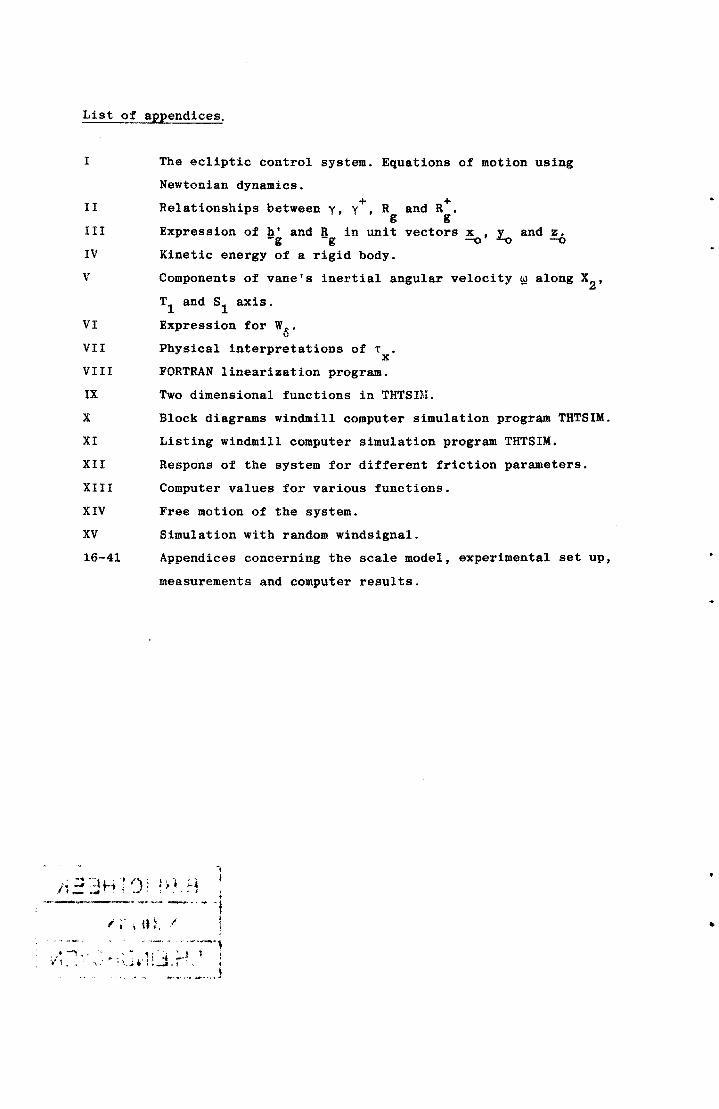
List of appendices.
I
II
III
IV
V
VI
VII
VIII
IX
X
XI
XII
XIII
XIV
XV
16-41
The ecliptic control system. Equations of motion using
Newtonian dynamics. + Relationships between y, y • R
g Expression of h' and R in unit -g -g Kinetic energy of a rigid body.
and R+. g
vectors .!o' 10 and .!o
Components of vane's inertial angular velocity ~ along X2 ,
Tl and 81 axis.
Expression for Woo
Physical interpretations of T • x
FORTRAN linearization program.
Two dimensional functions in THT8IM.
Block diagrams windmill computer simulation program THTSIM.
Listing windmill computer simulation program THT8IM.
Respons of the system for different friction parameters.
Computer values for various functions.
Free motion of the system.
Simulation with random windsignal.
Appendices concerning the scale model, experimental set uP.
measurements and computer results.
, -~ ~-I ' r)' \ 1 t..' h=~:.h' .~ t ~' ..• ,
"I I
i oM .... -;- - -- "'I
I ; \ H~. I I !
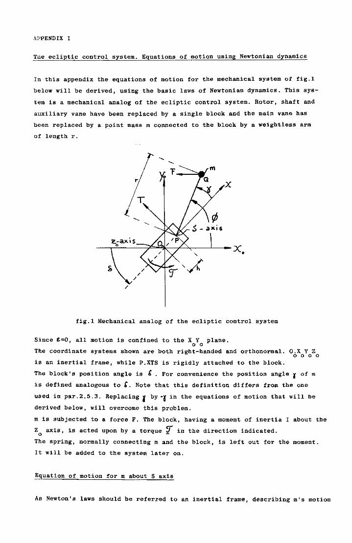
APPENDIX I
The ecliptic control system. Equations of motion using Newtonian dynamics
In this appendix the equations of motion for the mechanical system of fig.1
below will be derived, using the basic laws of Newtonian dynamics. This sys
tem is a mechanical analog of the ecliptic control system. Rotor, shaft and
auxiliary vane have been replaced by a single block and the main vane has
been replaced by a point mass m connected to the block by a weightless arm
of length r.
/
fig.1 Mechanical analog of the ecliptic control system
Since £=0, all motion is confined to the X Y plane. o 0
The coordinate systems shown are both right-handed and orthonormal. O.X Y Z o 0 0 0
is an inertial frame, while P.XTS is rigidly attached to the block.
The block's pOSition angle is 6 . For convenience the position angle ¥ of m
is defined analogous to 6. Note that this definition differs from the one
used in par.2.5.3. Replacing r bY·l in the equations of motion that will be
derived below, will overcome this problem.
m is subjected to a force F. The block, having a moment of inertia I about the
Z axis, is acted upon by a torque ~ in the direction indicated. o The spring, normally connecting m and the block, is left out for the moment.
It will be added to the system later on.
Equation of motion for m about Saxis
As Newton's laws should be referred to an inertial frame, describing m's motion
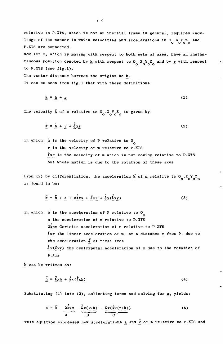
1.2
relative to P.XTS, which is not an inertial frame in general, requires know
ledge of the manner in which velocities and accelerations in 0 .X Y Z and o 000
P.XTS are connected.
Now let m, which is moving with respect to both sets of axes, have an instan
taneous position denoted by ~ with respect to 0 .X Y Z and by r with respect o 000
to P.XTS (see fig. 1).
The vector distance between the origins be ~.
It can be seen from fig.l that with these definitions:
k = h + r
The velocity k of m relative to 0 .X Y Z is given by: o 000
It = Ii + v + lxr
in which: Ii is the velocity of P relative to 0 0
v is the velocity of m relative to P.XTS
lxr is the veloci ty of m which is not moving relative
but whose motion is due to the rotation of these axes
(1)
(2)
to P.XTS
From (2) by differentiation, the acceleration k of m relative to 0 .X Y Z 000 0
is found to be:
in which:
..
k ..
2&xv + 'xr + tx<tXE.) = h + a + (3)
h is the accei:eration of P relative to 0 0
a the acceleration of m relative to P.XTS
2'xv Coriolis acceleration of m relative to P.XTS
€xr the linear acceleration of m, at a distance E. from P. due to
the acceleration , of these axes
tx(!XE.) the centripetal acceleration of m due to the rotation of
P.XTS
h can be written as:
(4)
Substituting (4) into (3), collecting terms and solving for~, yields:
a = k 2&xv fx(E.+~) ~. ~
A B
lx(!x(E.+~»
---------C
(5)
This equation expresses how accelerations a and k of m relative to P.XTS and
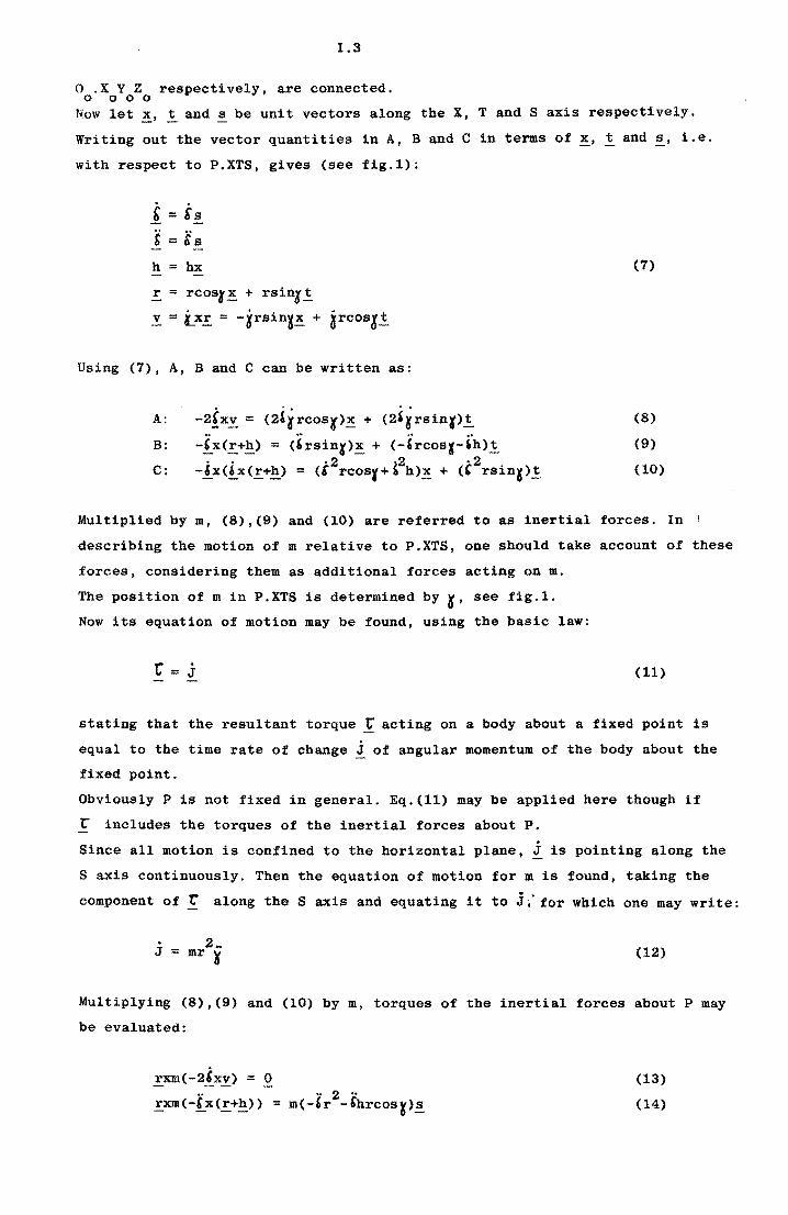
1.3
o .X Y Z respectively, are connected. o 000
Now let ~, ~ and ~ be unit vectors along the X, T and S axis respectively.
Writing out the vector quantities in A, Band C in terms of ~, t and~, i.e.
with respect to P.XTS, gives (see fig.l):
1 = Ss $ = Ss h :;; hx
!. = rcosK~ + rsinx~
Y = LX!. = -~rsin¥~ + ircosK~
Using (7), A, Band C can be written as:
A: -2!xy = (2'ircosl)~ + (2'irSinr)~ -Ix(!.+~)
.. ( -'rcosx-,'h)~ B: :;; (hsin¥)~ +
-!x(!.x(!.+!!.) ·2 ·2 ·2
C: = (6 rcosr+' h)~ + (' rsin,)~
(7)
(8)
(9)
(10)
Multiplied by m, (8),(9) and (10) are referred to as inertial forces. In I
describing the motion of m relative to P.XTS, one should take account of these
forces, considering them as additional forces acting on m.
The position of m in P.XTS is determined by ~, see fig.l.
Now its equation of motion may be found, using the basic law:
(11)
stating that the resultant torque ~ acting on a body about a fixed pOint is
equal to the time rate of change j of angular momentum of the body about the
fixed pOint.
Obviously p is not fixed in general. Eq.(ll) may be applied here though if
r includes the torques of the inertial forces about P.
Since all motion is confined to the horizontal plane, I is pointing along the
S axis continuously. Then the equation of motion for m is found, taking the
component of! along the S axis and equating it to j,' for which one may write:
2_ J = mr If (12)
Multiplying (8),(9) and (10) by m, torques of the inertial forces about P may
be evaluated:
!.xm(-21.xy) = 0
!.xm(-rx(!.+~) ) " 2 " = m(-'r -'hrcosr)~
(13)
(14)
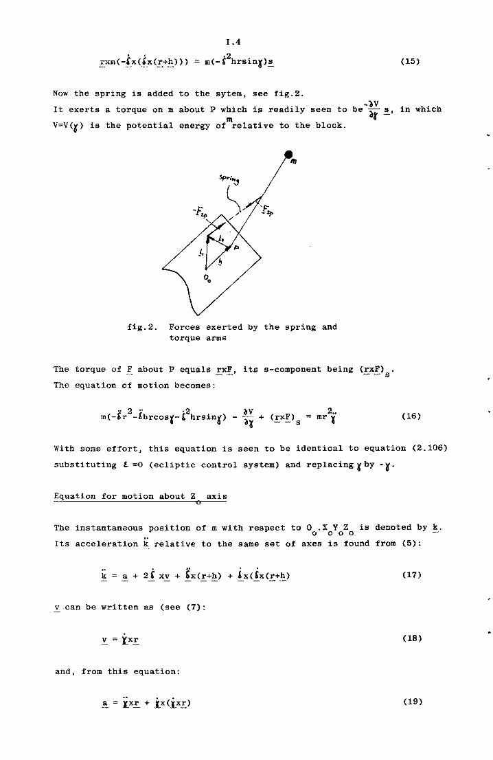
1.4
·2 m(-' hrsinK)~
Now the spring is added to the sytem, see fig.2.
(15)
-lV It exerts a torque on m about P which is readily seen to be ~ s, in which 111 r-
V=V(~) is the potential energy of relative to the block.
fig.2. Forces exerted by the spring and torque arms
The torque of ! about P equals rx!, its s-component being (~x!)s.
The equation of motion becomes:
(16)
With some effort, this equation is seen to be identical to equation (2.106)
substi tuting E.. =0 (ecliptic control system) and replacing t by -r.
Equation for motion about Z axis o
The instantaneous position of m with respect to 0 .X Y Z is denoted by ~. o 000 ..
Its acceleration k relative to the same set of axes is found from (5):
(17)
v can be written as (see (7):
v = txr (18)
and, from this equation:
(19)
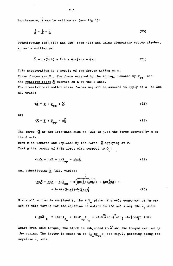
1.5
Furthermore, , can be written as (see fig.l):
!=1-i (20)
substituting (18),(19) and (20) into (17) and using elementary vector algebra,
k can be written as:
(21)
This acceleration is a result of the forces acting on m.
These forces are! , the force exerted by the spring, denoted by F ,and -sp the reactive force ~ exerted on m by the Saxis.
For translational motion these forces may all be assumed to apply at m, so one
may write:
or:
mk=F+F +.R -sp
-1< = F + F ..
-mk -sp
(22)
(23)
The force -~ at the left-hand side of (23) is just the force exerted by m on
the Saxis.
Next m is removed and replaced by the force -8 applying at P.
Taking the torque of this force with respect to 0 : o
-hxR= hxF + hxF - mhxk - -sp
and substituting k (21), yields: o II
-~xB = ~x! + EX!ap - m[ix(l:(!.x~» + hx(fX~) +
+ ~x(tx(tXE.) )+~(ixE.)]
(24)
(25)
Since all motion is confined to the X Y plane, the only component of intero 0
est of this torque for the equation of motion is the one along the Z axis: o
2"'2 .. = (hxF) + (hxF ) + m(-h b+hr+ sin~ -hr,cosy) (26) - - Zo - -sp Zo 0
Apart from this torque, the block is subjected to ~ and the torque exerted by
the spring. The latter is found to be.(11xF ), see fig.2, pointing along the - -sp
negative Z axis. o
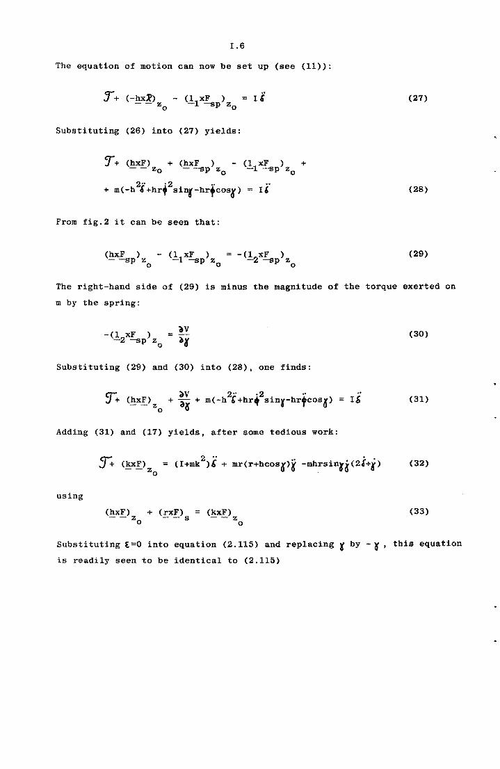
1.6
The equation of motion can now be set up (see (11»:
- (llXF ) = I' - -sp zo
(27)
Substituting (26) into (27) yields:
Jr+ (hxF) + (hxF) - (llxF ) + - - Zo - -sp Zo - -sp zo
2"'2 ., + m(-h ~+hr+ sinr-hr+cosK) :::: U (28)
From fig.2 it can be seen that:
(hxF ) - (llxF ) = -(1 xF ) - -sp Zo - -sp Zo -2 -sp Zo
(29)
The right-hand side of (29) is minus the magnitude of the torque exerted on
m by the spring:
(30)
Substituting (29) and (30) into (28), one finds:
r+ (hxF) --z (31)
o
Adding (31) and (17) yields, after some tedious work:
~ (~X!)z = (I+mk2)€ + mr(r+hcosK)i -mhrSin¥~(2i+i) (32)
o .
using
(hxF) + (rxF) - - zo - - s
:::: (kxF) --z
o (33)
Substituting £=0 into equation (2.115) and replacing r by -l' this equation
is readily seen to be identical to (2.115)
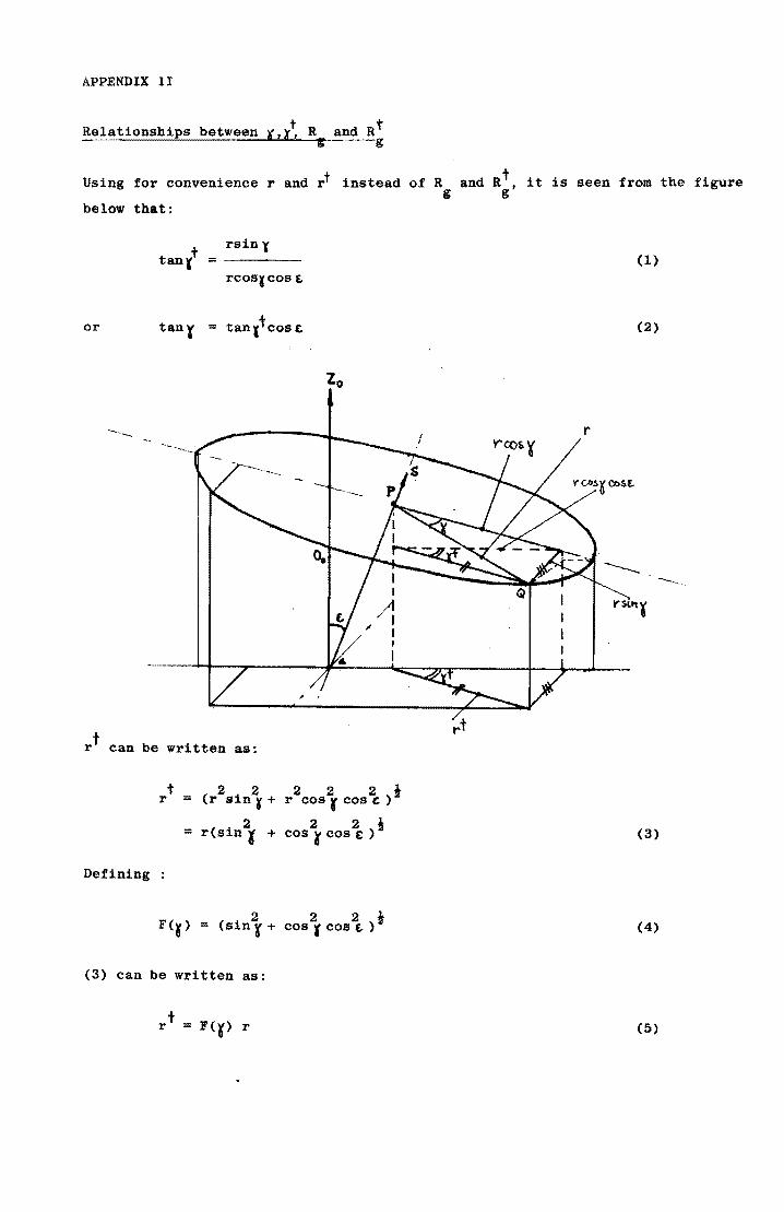
APPENDIX II
t Relationships between (,X, R and Rt g
Using for convenience rand rt instead of Rand Rt it is seen from the figure g g'
below that:
tan .,.t rsin~
= rcosxcos E-
or tan't ;; tanltcost.
"'---
rt can be written as:
t 2 2 r = (r sin ¥ +
2 = resin r +
Defining
(3) can be written as:
20
2 2 2! r cos r cos t! )
2 2! cos r cos t )
(1)
(2)
(3)
(4)
(5)
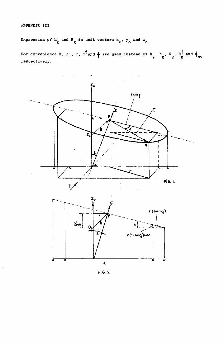
APPENDIX III
Expression of h' and R in unit vectors x ,y and z -g -- -g -0 "'"'0 -- -0
For convenience h, h', r, rtand & are used instead of h , h', R , Rt and! T g g g g Tmv
respectively.
-- ----..:..
--A
FIG. 1.
s
A B
FiG. 2.
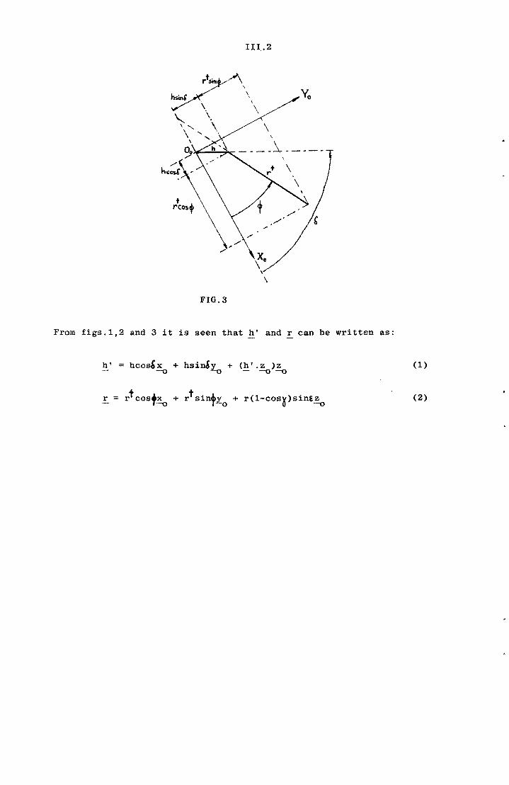
UI..2
r~\ ~ \
,,\. \ \" \ \ \"' .
\ " . ""~
\
FIG.3
From figs.1,2 and 3 it is seen that h' and r can be written as:
h' = hCos&~ + hsinbv + (h'.z )z v "'-0 - -0-0
(1)
(2)
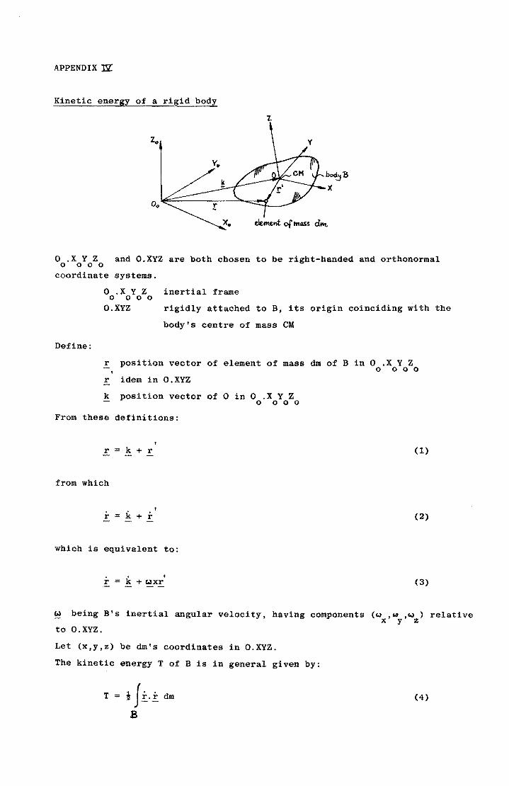
APPENDIX nz:
Kinetic energy of a rigid body
o .X Y Z 000 0
and O.XYZ are both chosen to be right-handed and orthonormal
coordinate systems.
o .X Y Z inertial frame o 000
O.XYZ rigidly attached to B, its origin coinciding with the
body's centre of mass eM
Define:
r position vector of element of mass dm of B in 0 .X Y Z o 000
r
k
idem in O.XYZ
position vector of 0 in 0 .X Y Z o 000
From these definitions:
r = k + r
from which
r = k + r
which is equivalent to:
r = It + c.:Ixr'
(1)
(2)
(3)
w being B's inertial angular velocity. having components (Q ,Q .~ ) relative x y z
to O.XYZ.
Let (x,y,z) be dm's coordinates in O.XYZ.
The kinetic energy T of B is in general given by:
T = i Ji.i dm (4)
B
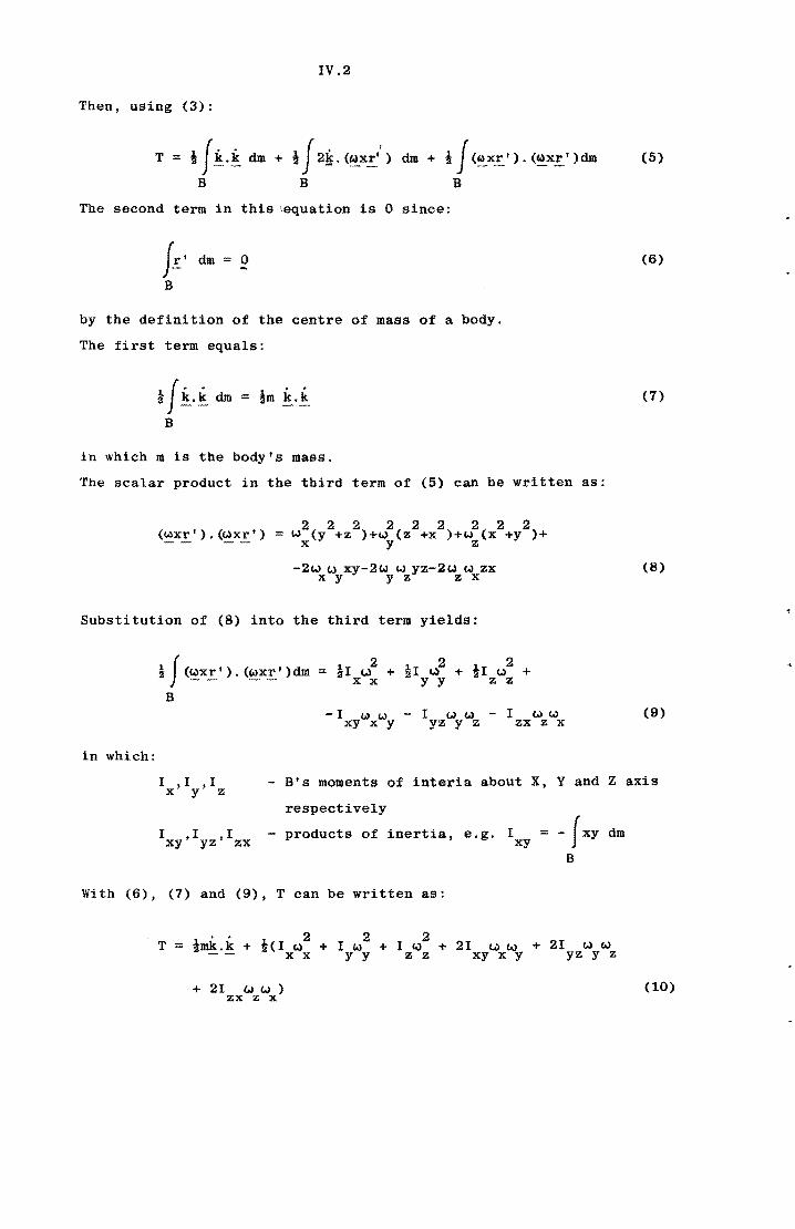
IV.2
Then, using (3);
T = i J !.. i dIn + i f 2~. (~xi ) B B
dm + 1 J (~x.!:.'). (~x!.·)dIn B
The second term in this :equation is 0 since:
f.!:.' dm = 0
B
by the definition of the centre of mass of a body.
The first term equals:
i f i·~ dm = im i·~ B
in which m is the body's mass.
The scalar product in the third term of (5) can be written as:
(~x.!:.'). (~xr') 222 222 222 = w (y +z )+w (z +x )+w (x +y )+ x y z
-2w w xy-2w w yz-2w w zx x y y z z x
Substitution of (8) into the third term yields:
i f (~xr I ) • (~x.!: I ) dm = i I ,i + i I (.)2 + 1 I w2
+ x x y y z z B
-I (.,) w - I (,) w - I w w xy x y yz y z zx z x
in which:
1 • I • I x Y z
- B's moments of interia about X,
I I I xy' yz' zx
respectively
products of inertia,
With (6), (7) and (9), T can be written as:
e.g. I xy
Y and
- [xy
B
Z
dm
. . 222 T = lmk.k + 1(1 w + 1 w + 1 w + 21 ~ w + 21 w w x x y y z z xy x y yz y z
(5)
(6)
(7)
(8)
(9)
axis
+ 21 w w ) (10) zx z x
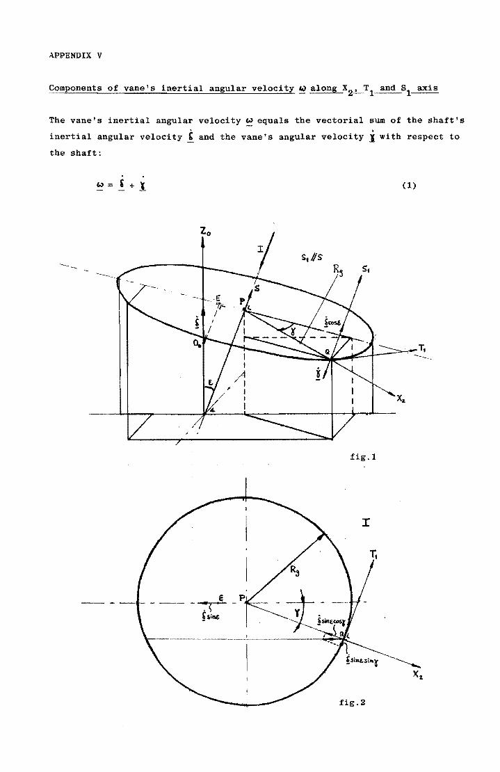
APPENDIX V
Components of vane's inertial angular velocity ~ along X2_._T1 and 81 axis
The vane's inertial angular velocity ~ equals the vectorial sum of the shaft's
inertial angular velocity' and the vane's angular velocity i with respect to
the shaft:
. w = ~ + I (1)
fig.1
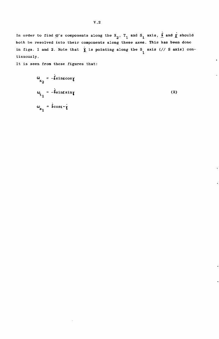
V.2
In order to find ~'s components along the x2
' Tl and Sl axis, , and X should
both be resolved into their components along these axes. This has been done
in figs. 1 and 2. Note that
tinuously.
1 is pointing along the S axis (II Saxis) con-1
It is seen from these figures that:
(.J = -!sin£cos~ x2
G.>t -6'sintsinl (2) 1
w bCOSE-"i sl
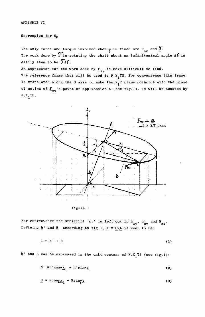
APPENDIX VI
Expression for Y!.$
The only force and torque involved when y is fixed are F and ~ o -mv-The work done by ~in rotating the shaft about an infinitesimal angle 4' is
easily seen to be 5fA'. An expression for the work done by F is more difficult to find.
-mv The reference frame that will be used is P.X1TS. For convenience this frame
is translated along the S axis to make the X1
T plane coincide with the plane
of motion of F 's point of application L (see fig.I). It will be denoted by -mv
K.X1TS.
fmv..l. ~ and. in 'X. T plQrlc.
figure 1
For convenience the subscript 'mv' is left out in h h' and R mv' mv mv
Defining h' and R according to fig.I, 1:= Qo~ is seen to be:
1 = h' + R (1)
h' and R can be expressed 1'n th it f K X TS ( 1 e un vectors 0 • 1 see fig. ):
h' =h'cOS«~l + h'si~s (2)
(3)
VI.2
Substitution of (2) and (3) into (1) yields:
l={h'COS~+RcOSX)~1 +h'sinus - RSinr! (4)
When the shaft is rotated this vector will not undergo any change in magni
tude since K is fixed. Its direction in inertial space is affected though,
since ~1' t and s change directions.
These changes in ~1' t and s are found as follows.
The components of an inertial angular velocity! in
The time rates of change of ~1' t and s are then found
· £x~l tcosLt ~1
· &xt -'cos£~1 'siIll s t :; :;
· 'xs 6 sin£ t s :;
from which:
to be:
(5)
(6)
fig.I).
Any change 41 in ! due to a change in , can, provided ( is fixed, be expressed
by (from (-4) :
Al =
Substituting (6) into (7) yields:
Finally. expressing F in ~1' t and s (see fig.l): -mv
F :; -F sintx - F cosvt -mv mv B-1 mv 0-
(7)
(8)
(9)
, the work F .Al done by F in rotating the shaft about an ang1eA'is found: -mv -mv
VI.3
F .41 = -(Rcos,+hcosr)F -mv - 0 mv
using (see fig.1):
h = h' (COSd.cos e. + sinG(sin&)
= htcos(cC-t)
(10)
(11)
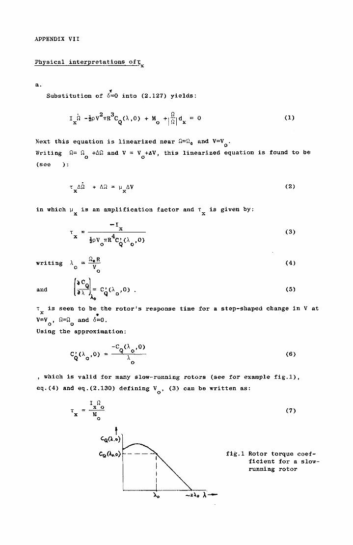
APPENDIX VI I
Physical interpretations of~ x
a. y
Substitution of 0=0 into (2.127) yields:
(1)
Next this equation is linearized near Q=Qo and V=V . o Writing Q= Q +~Q and V = V +AV, this linearized equation is found to be
o 0
(see ) :
jJ ~V x
(2)
in which JJx
is an amplification factor and Tx is given by:
-1 T = ________ ~x~ __ __
x ipv WR4CQ'(A ,0)
o 0
(3)
writing A = QoR o V
(4) o
and (5)
T is seen to be the rotor's response time for a step-shaped change in V at x
V=V 0'
Using
it
Q=Q and 0=0. o
the approximation:
-C (A ,0) C'(A 0) = Q 0
Q 0' A o
(6)
, which is valid for many slow-running rotors (see for example fig.1),
eq.(4) and eq.(2.130) defining Vo
' (3) can be written as:
I Q x 0
T =--x M
o
t ~(l.o)
Cg(Ao.o)
(7)
fig.1 Rotor torque coefficient for a slowrunning rotor
VII .2
b.
Consider a situation in which the rotor has an angular speed n and in o
which V=V • o
Now suppose V to drop to 0 suddenly and the rotor to be subjected to a torque
M at the same time. Neglecting aerodynamic damping, its equation of motion o
is then given by:
I n + M o x 0
Using n.= nino' the solution to this differential equation is:
M o
1 - I n t x 0
(8)
(9)
(7) is then seen to equal the reciprocal time rate of decrease of QM'
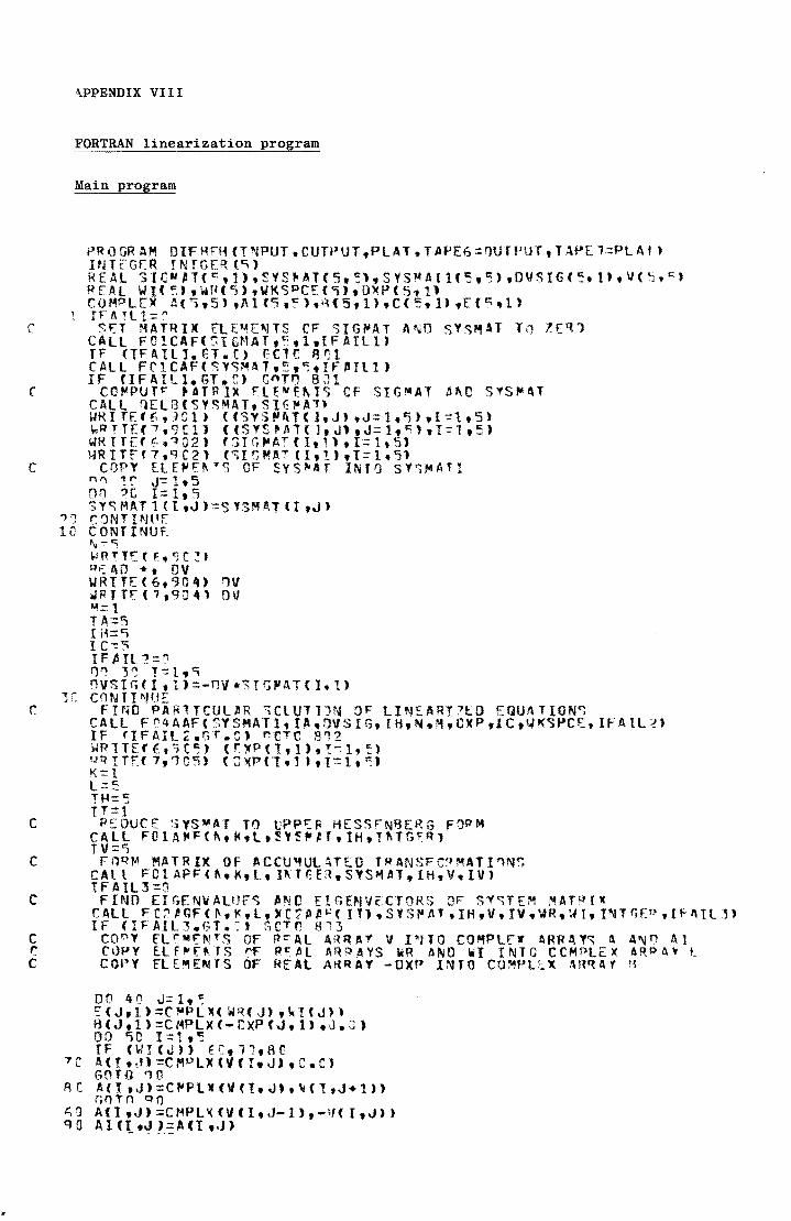
\PPENDIX VIII
FORTRAN linearization program
Main program
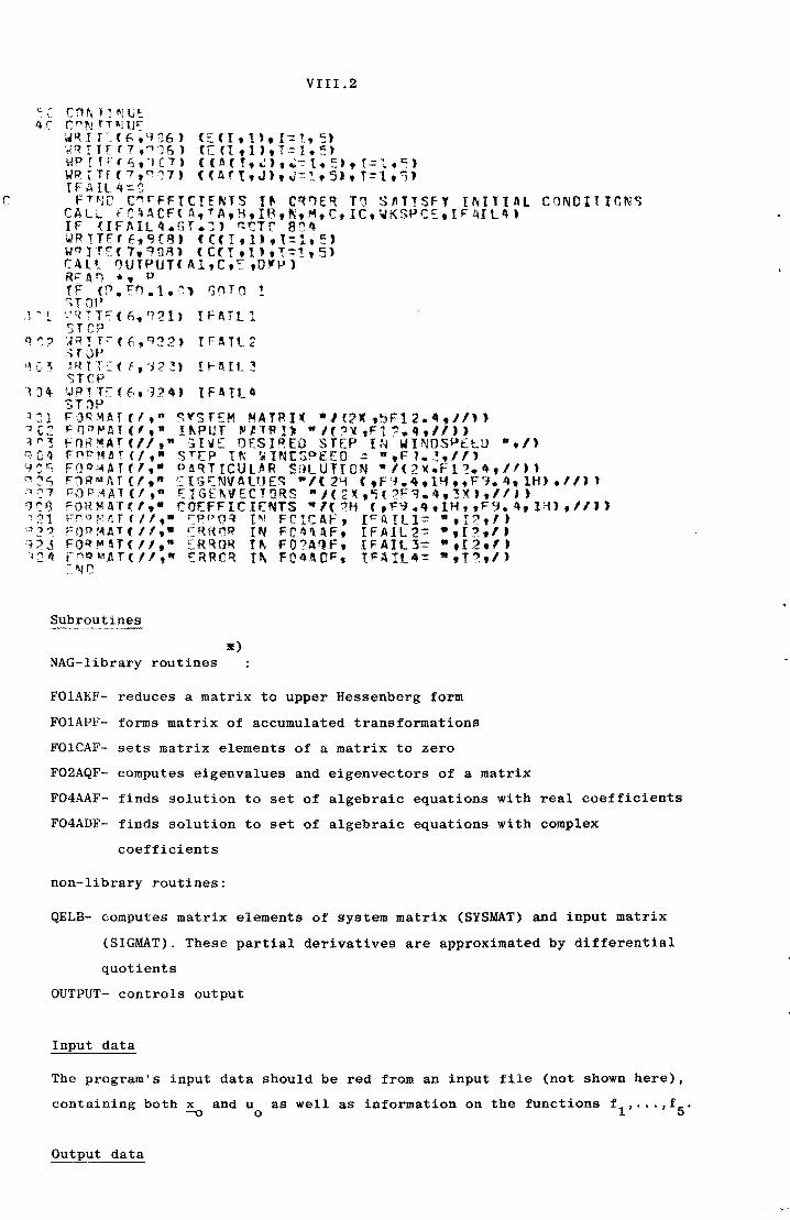
VIII,2
"';: cnr-.lTlIlU': 4C ~"~JrHjtJt::
'I'"
W~Ir (f"QQ6)
',I q r r 1: f 7 .'" 'J t. 1 Wp r T E ( I) t 1 C 7 , YR IT f{ 7, r:'I I) 7) IFAIL4-=!J FT~r c"rfFICIfNTS t~ Cq~ER TO SATISFY INITIAL CONDITIONS
CALL FC4ACF(A,TAtR,IBtNt~,CtIC,WKSPCEtIF4IL.} IF (IFAIl~.Gr.;l ~tTr ary4 wR1Tf(E,~(q) (((rtl)tt=l,~) WOIT[f1,9QA) (C(T,1'.T-=1,5) CALt QUTPUT(Al,Ct~,D'p) R~ A 11 .. , P IF (P.t:"O.l.~l GI')TO!. 'iTOP
r~ TT:: ( f;. 921) IF 1\ J l 1 STep ~qtT~(f,~22) IFayt2 "rJP J~nT_(ft'J2~) Irl\rl~ STep VPyT[(f.924) IF_tl4 ST :W ~Jq~ATCI,- ~YsrEM MATRI_ ·/(2X,5F12.4,1!" FOOPAT(f,· I~PUT ~'l~I) ·'('X,Fl~.4,11}) FORMAT(II,· iIVE OESIRED STEP IN WINDSPE~U ·,/) Fn~Mlf(/t- STEP IN ~lN[SPEEO ~ ·,Fl.~tll)
4Sr.; "1:;6 -'~7
'JS8 , 21 '12 , '':; 2.3
Fog~Ar(/,· PA~TICUl.R S~lUTION ·/(2~.Fl?4,1") F1RMAf(I,- ;::IG::::NVAUJ£~ "/[2!-f (,F'1.4.Ui .. F'j.4.1H) ,II) FOP~AT(/tft EIGE~VECTORS ftJ(2K,~(2Fq.4,3~),'lj) FORMAT(/,· COEFFICIENTS ·/(~H (,F9.4.1H"FY.4,lH),II') F~q~aT(I',· ~P"Oq 1M FCICAF, I~Alll= ·,12", FOOMAT(/f,- ~~HOR IN FC"AF. [fAll2= ·,12.1' FOq~~T(",· £RQOR T~ F02AQF, IFAIl3= ",I2,f' f"QMAT(II,· ERRCR r~ F04~CFt tFAIl4= -,12,/) ~~Q
Subroutines
NAG-library routines
FOIAKF- reduces a matrix to upper Hessenberg form
FOIAPF- forms matrix of accumulated transformations
FOICAF- sets matrix elements of a matrix to zero
F02AQF- computes eigenvalues and eigenvectors of a matrix
F04AAF- finds solution to set of algebraic equations with real coefficients
F04ADF- finds solution to set of algebraic equations with complex
coefficients
non-library routines:
QELB- computes matrix elements of system matrix (SYSMAT) and input matrix
(SIGMAT). These partial derivatives are approximated by differential
quotients
OUTPUT- controls output
Input data
The program's input data should be red from an input file (not shown here),
containing both ~ and Uo
as well as information on the functions f 1 ,· ",f5 ,
Output data
VIII .3
fhe program's output consists of the system and input matrix, the desired
step in wind speed. the particular solution, the eigenvalues and eigenvec
tors of the system matrix. the coefficients of the final solution (£) and
6x as a function of time.
Version Mark 6 April 1978
Distributor:
The business manager
NAG Central Office
7 Banbury Road
Oxford OX2 6NN
United Kingdom
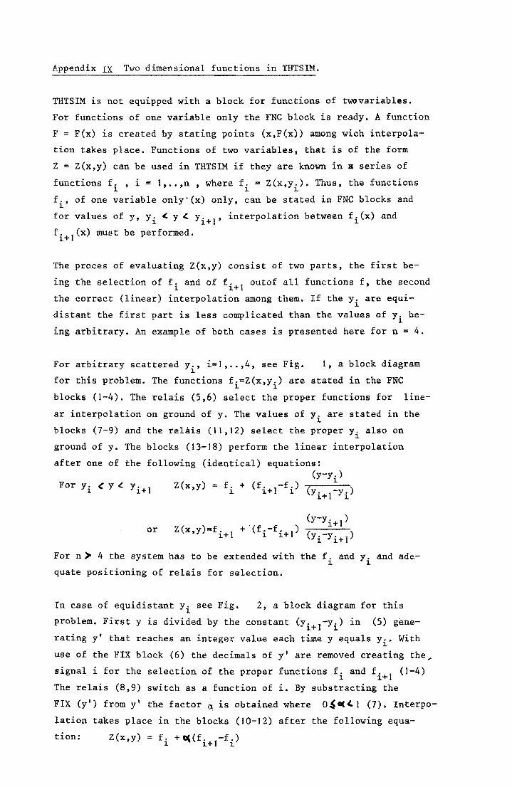
Appendix IX Two dimensional functions 1n THTSIM.
THTSIM is not equipped with a block for functions of twovariables.
For functions of one variable only the FNC block is ready. A function
F = F(x) is created by stating points (x,F(x» among wich interpola
tion takes place. Functions of two variables, that is of the form
Z = Z(x,y) can be used in THTSIM if they are known in a series of
functions f. , i = I, •• ,n , where f. = Z(x,y.). Thus, the functions 111 f., of one variable only'(x) only, can be stated in FNC blocks and
1
for values of y, Yi < y < Yi+l' interpolation between fi(x) and
f. I(x} must be performed. 1+
The proces of evaluating Z(x,y) consist of two parts, the first be
ing the selection of f. and of f. 1 outof all functions f, the second 1 1+
the correct (linear) interpolation among them. If the y. are equi-1
distant the first part is less complicated than the values of y. bel.
ing arbitrary. An example of both cases is presented here for n = 4.
For arbitrary scattered y., i=I, •• ,4, see Fig. l.
for this problem. The functions f.=Z(x,y.) are
I, a block diagram
stated in the FNC l. l.
blocks (1-4). The relais (5,6) select the proper functions for line-
ar interpolation
blocks (7-9) and
ground of y. The
after one of the
on ground of y. The values of y. are stated in the l.
the re1Ais (11,12) select the proper y. also on l.
blocks (13-18) perform the linear interpolation
following (identical) equations:
For y. < y <: y. 1 1. 1.+
(y-Yi) Z(x,y) = f. + (f. I-f.) ( )
l. 1.+ 1. Yi+I-Yi
(y-y i+1) or Z(x,y)=f. 1 + (f.-f·+ 1) ( )
1.+ l. l. Yi-Yi+l
For n> 4 the system has to be extended with the f. and y. and ade-1. 1.
quate positioning of re1ais for selection.
In case of equidistant Yi see Fig. 2, a block diagram for this
problem. First y is divided by the constant (Yi+l-Yi) in (5) gene
rating y' that reaches an integer value each time Y equals y .• With 1. use of the FIX block (6) the decimals of y' are removed creating the,
signal i for the selection of the proper functions f. and f. 1 (1-4) 1. l.+
The relais (8,9) switch as a function of i. By substracting the
FIX (y') from y' the factor ex is obtained where O",OC<'1 (7). Interpo
lation takes place in the blocks (10-12) after the following equa-
tion: Z(x,y) = + C( (f. 1-f.) l.+ 1.
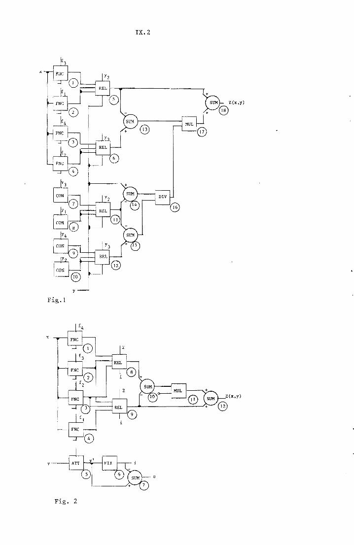
IX.2
SUM Z( f,;;\ x,y)
r---l I + ~ I MUL r-::
@
Fig.l
y-
Fig. 2
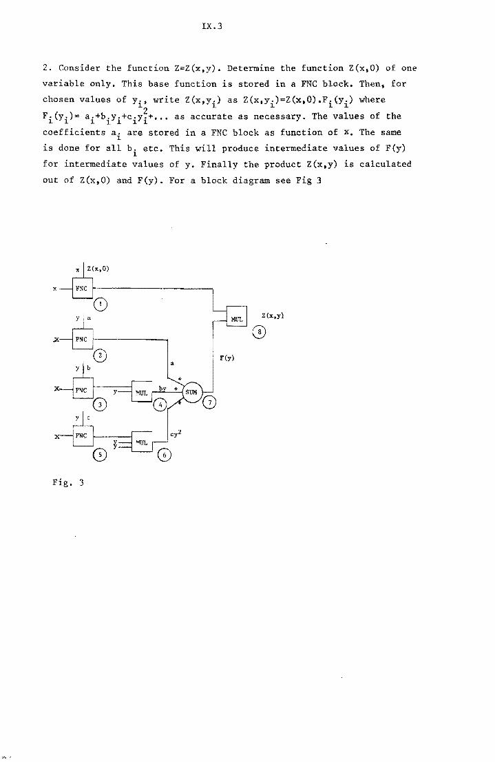
IX.3
2. Consider the function Z=Z(x,y). Determine the function Z(x,O) of one
variable only. This base function is stored in a FNC block. Then, for
chosen values of y., write Z(x,y.) as Z(x,y.)=Z(x,O).F.(y.) where ~2 ~ ~ ~ 1
F.(y.): a.+b.y.+c.y.+ ••• as accurate as necessary. The values of the ~ ~ 111 1 1
coefficients a i are stored in a FNC block as function of x. The same
is done for all b. etc. This will produce intermediate values of F(y) 1
for intermediate values of y. Finally the product Z(x,y) is calculated
out of Z(x,O) and F(y). For a block diagram see Fig 3
F(y)
Fig. 3
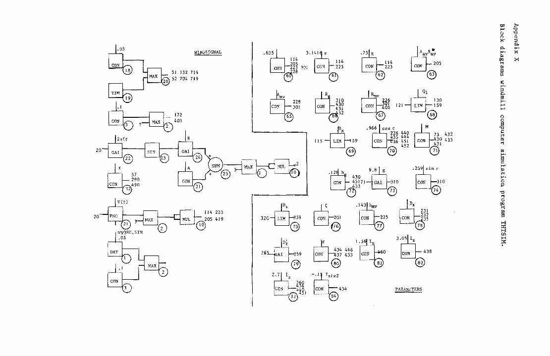
t:d :l>-I-' "0 0 "0 (l (1)
l'" ::; 0..
WINDSIGNAL o"Q '-'8 Gl:' 0.. .....
Gt ..... :<
114 114 III
114 ()Q ::<
CON d~i 301 CON ~23 CON 223 CON 205 t1 III
J32 714 ® a 704 719
62 CJ)
~ .....
El ~H :::I
E1: 0..
228 310 CON ~~ 121 LIM :~~
a CON 301 CON 430
..... I-'
43J I-'
172 ® ~32 ® ® 403 (l 0
n'B" ~ ~
73 432 c:: r1'
CON 30 433 (I)
431 t1
20 ® @ til ..... ~
08 H Tl"b I-' III
430 r1' .....
CON 43171 GAl 310 CON 310 0
6 3
® @ P
7 73 "0 t1
-fb Q 0 e201
()Q
114 223 231 t1
20 III
320 LIM 59 CON dJ~ a
@ @ 78 t-':l
I i"~O"M ::r:: t-':l
.05 30
Q til
~ ~ H
26 Al Z 59
~
"" 1 ~ 434 446 CON 438 CON 37 453
~~ @ @ @
CON 3 2 2~ bh t~~ CON 4*gl CON 434 PARAMETERS
® ®
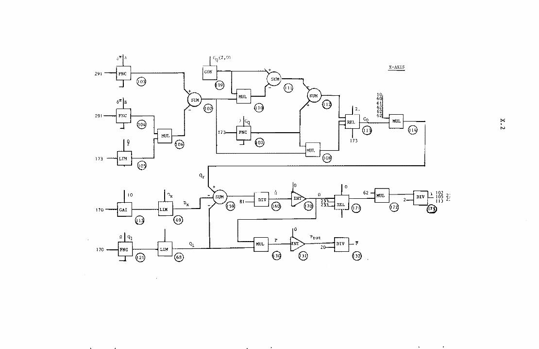
X-AXIS 291
291
N
173
173
170
170
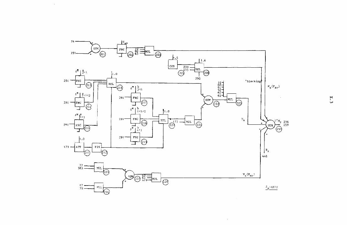
76---""","
291--_
29l
29l
WX~<l I
2Ql FNC '
173
77 383
67 70
~15
'blocking
+
448
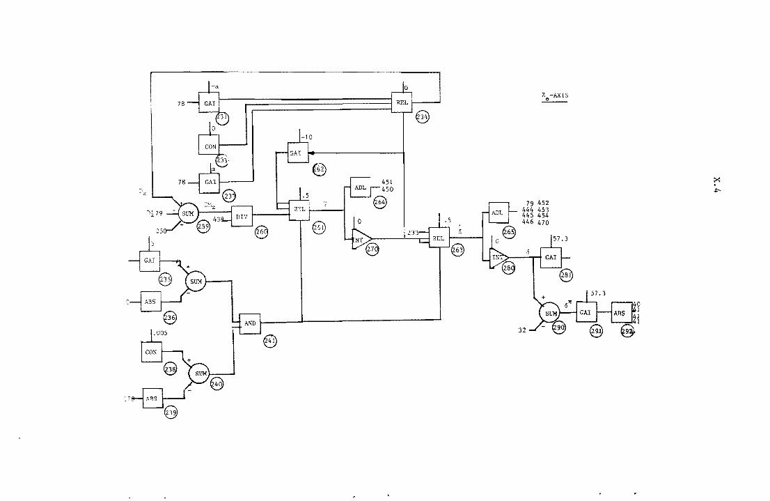
Z-AXIS .0. __
79 452 444 453 445 454 446 470
32
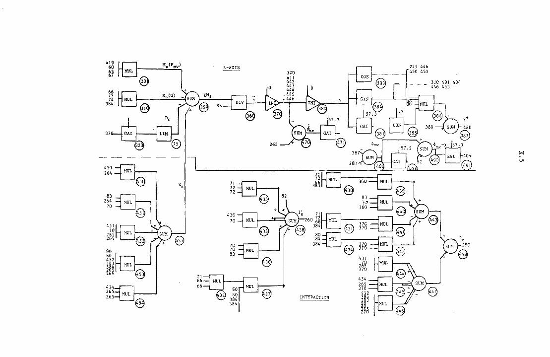
419 Ms(Fmv) 60 S-AXIS 225 446
~1 450 453
@ 310 431 434 0 - - - 446 453
66 Ms(G) 73
74 384 e 37
~ - --
Ln
430 264 H e Rs 71 3M 72
72 83 82
264 70
70 431
70 265 80 265 84
70E] 384
80 70 MUL 80 83 432 e 431
~n j~~ 71 66
434 66 265
30 @ 265 e 384 INTERACTION
384
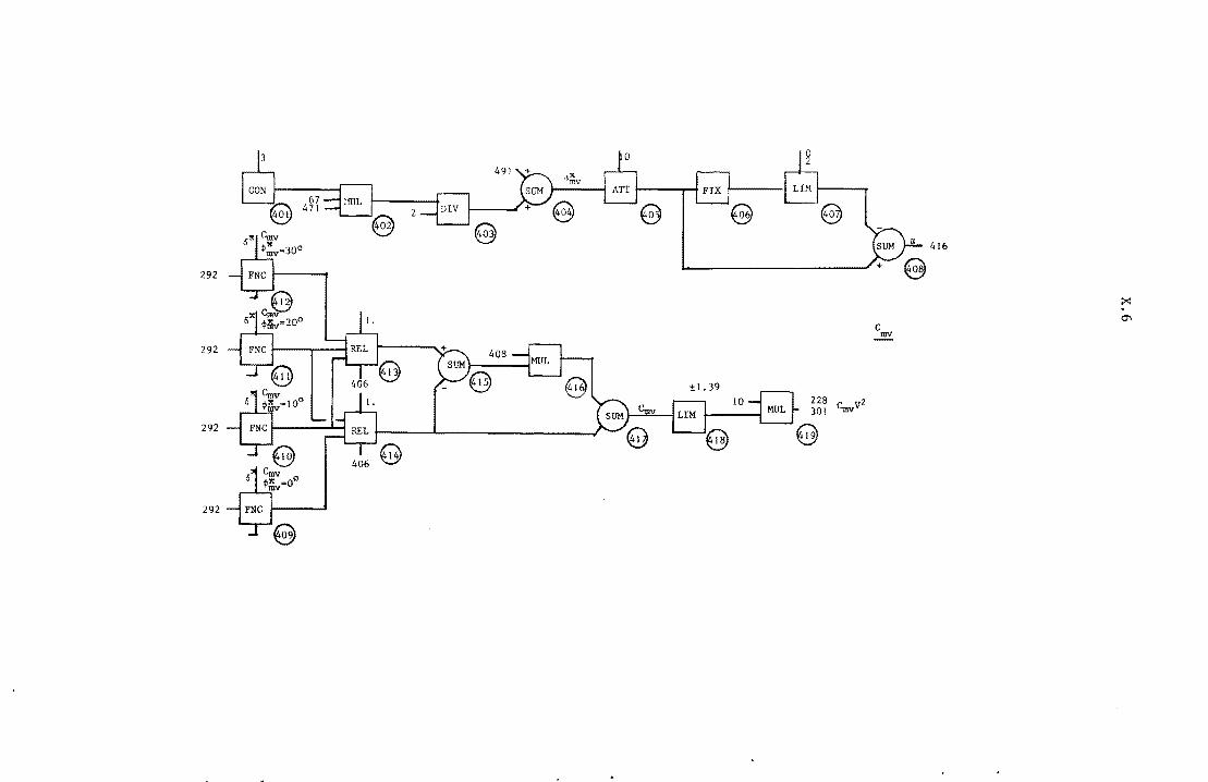
292
292
292
292
±1. 39
406
228 (' V2 30l '"'IllV
416
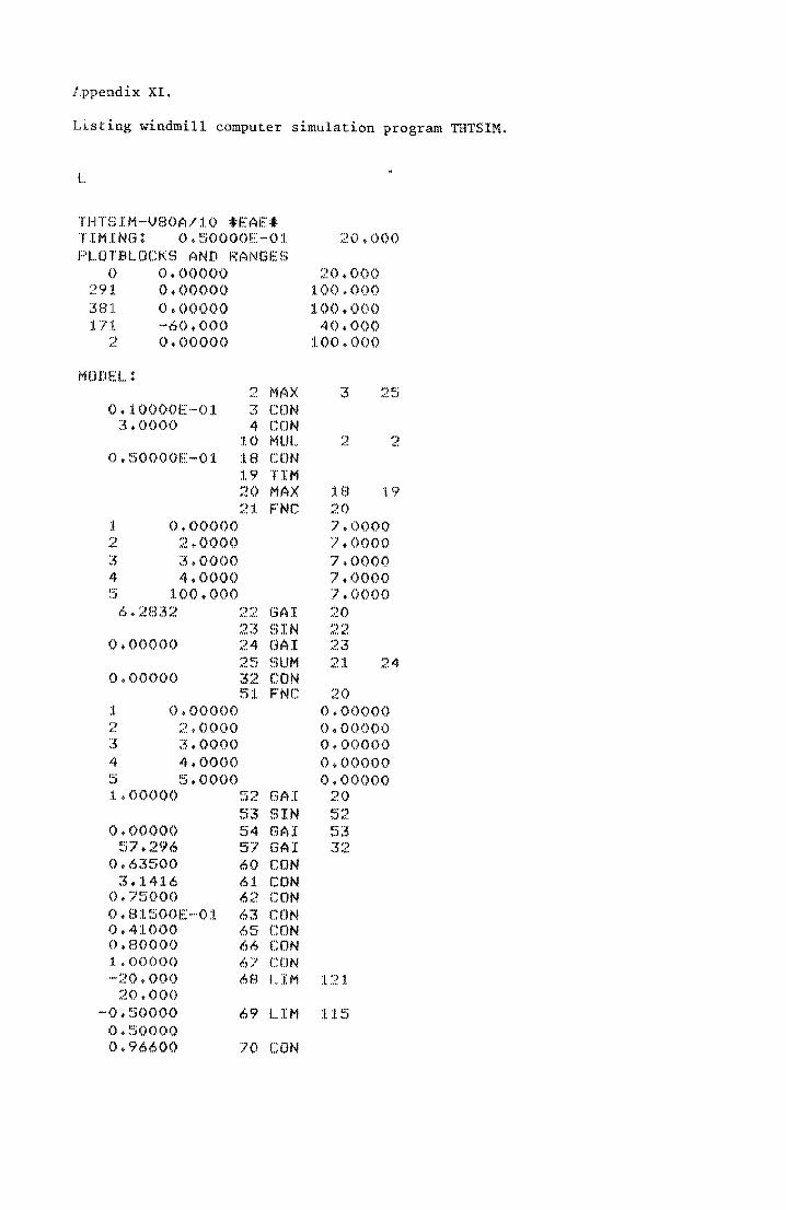
f~pendix XI.
Listing windmill computer simulation program THTSIM.
L
THTSIM-V80A/10 IEAEI TIMING: 0.50000E-01 20.000 PLOTBLOCKS AND RANGES
0 0.00000 20.000 291 0.00000 100.000 381 0.00000 100.000 171 -60.000 40.000
2 0.00000 100.000
MODELl 2 MAX 3 ~~ ,J
0.10000E-Ol 3 CON 3.0000 4 CON
10 MUL ~ , 2 0.50000E-Ol 18 CON
19 TIM 20 MAX 18 19 21 FNC 20
1 0.00000 7.0000 2 2.0000 7.0000 3 3.0000 7.0000 4 4.0000 7.0000 5 100.000 7.0000
6.2832 22 GAl 20 23 SIN 22
0.00000 24 GAl 23 ~~ ,J SUM 21 24
0.00000 32 CON 51 FNC 20
1 0.00000 0.00000 2 2.0000 0.00000 3 3.0000 0.00000 4 4.0000 0.00000 ~ J 5.0000 0.00000 1.00000 52 GAl 20
53 SIN 52 0.00000 54 GAl 53
57.296 57 GAl 32 0.63500 60 CON
3.1416 61 CON 0.75000 62 CON 0.81500E-01 63 CON 0.41000 65 CON 0.80000 66 CON 1.00000 67 CON -20.000 68 LIM 121
20.000 -0.50000 69 LIM 115
0.50000 0.96600 70 CON
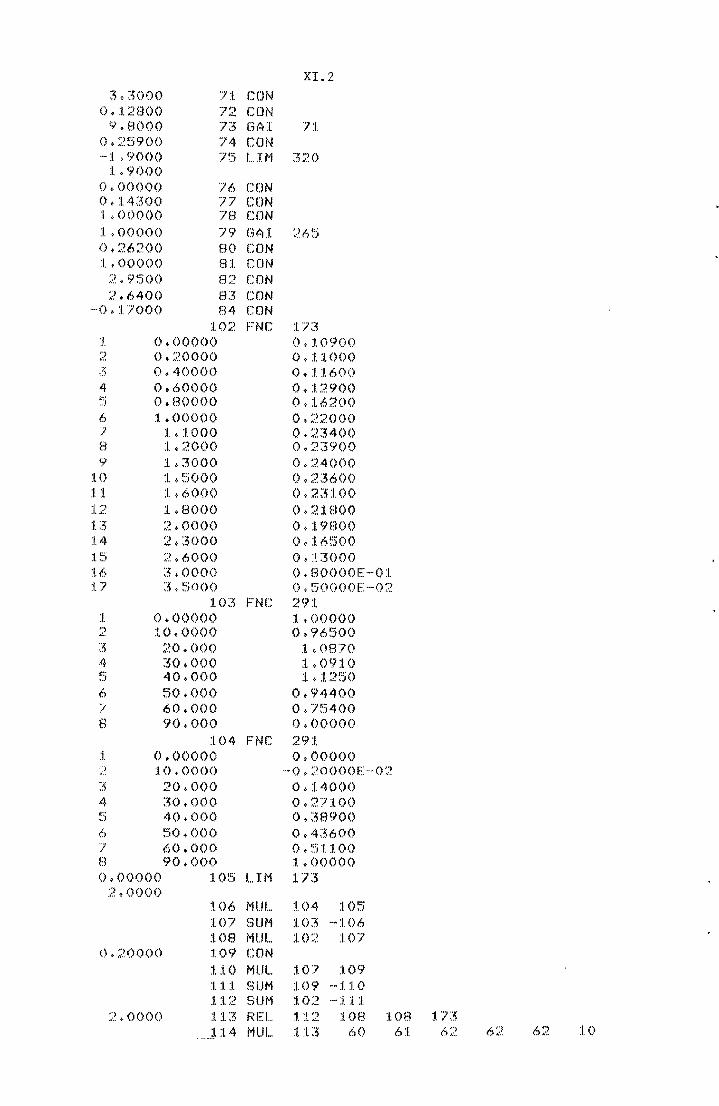
XI.2 3.3000 71 CON
0.12800 72 CON 9.8000 73 GAl 71
0.25900 74 CON -1.9000 75 LIM 320
1.9000 0.00000 76 CON 0.14300 77 CON 1.00000 78 CON 1.00000 79 GAl 265 0.26200 80 CON 1.00000 81 CON
2.9500 82 CON 2.6400 83 CON
-0.17000 84 CON 102 FNC 173
1 0.00000 0.10900 2 0.20000 0.11000 3 0.40000 0.11600 4 0.60000 0.12900 ~ J 0.80000 0.16200 6 1.00000 0.22000 7 1.1000 0.23400 8 1.2000 0.23900 9 1.3000 0.24000
10 1.5000 0.23600 11 1.6000 0.23100 12 1.8000 0.21800 13 2.0000 0.19800 14 2.3000 0.16500 15 2.6000 0.13000 16 3.0000 O.BOOOOE-Ol 17 3.5000 0.50000E-02
103 FNC 291 1 0.00000 1.00000 ~ , 10.0000 0.96500 3 20.000 1.0870 4 30.000 1.0910 ~ J 40.000 1.1250 6 50.000 0.94400 7 60.000 0.75400 8 90.000 0.00000
104 FNC 291 1 0.00000 0.00000 ~ 10.0000 -0.20000E-02 L
3 20.000 0.14000 4 30.000 0.27100 5 40.000 0.38900 6 50.000 0.43600 7 60.000 0.51100 8 90.000 1.00000 0.00000 105 LIM 173
2.0000 106 MUL 104 105 107 SUM 103 -106 108 MUL 102 107
0.20000 109 CON 110 MUL 107 109 111 SUM 109 -110 112 SUM 102 -111
2.0000 113 REL 112 108 108 173 114 MUL 113 60 61 62 62 62 10
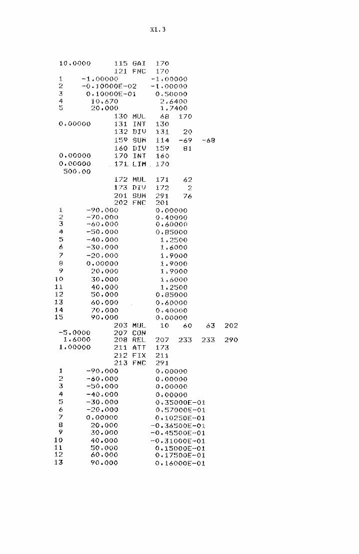
XI.3
10.0000 115 GAl 170 121 FNC 170
1 -1.00000 -1.00000 ~ -0.10000E-02 -1.00000 • 3 0.10000E-01 0.50000 4 10.670 2.6400 ~ J 20.000 1.7400
130 MUL 68 170 0.00000 131 INT 130
132 DIV 131 20 159 SUM 114 -69 -68 160 DIV 159 81
0.00000 170 INT 160 0.00000 171. LIM 170
500.00 172 MUL 171 6? -173 DIV 172 2 201 SUM 291 76 202 FNC 201
1 -90.000 0.00000 ~ , -70.000 0.40000 3 -60.000 0.60000 4 -50.000 0.85000 ~ J -40.000 1.2500 6 -30.000 1.6000 7 -20.000 1.9000 8 0.00000 1.9000 9 20.000 1.9000
10 30.000 1.6000 11 40.000 1.2500 12 50.000 0.85000 13 60.000 0.60000 14 70.000 0.40000 1~ J 90.000 0.00000
2()3 MUL 10 60 63 202 -5.0000 207 CON
1.6000 208 REL 207 233 233 290 1.00000 211 ATT 173
212 FIX 211 213 FNC 291
1 -90.000 0.00000 ~ • -60.000 0.00000 3 -50.000 0.00000 4 -40.000 0.00000 5 -30.000 0.35000E-Ol 6 -20.000 0.57000E-Ol 7 0.00000 0.10250E-01 8 20.000 -0.36500E-Ol 9 30.000 -0.45500E-Ol
10 40.000 -0.31000E-01 11 50.000 0.15000E-01 12 60.000 0.17500E-Ol 13 90.000 0.16000E-Ol
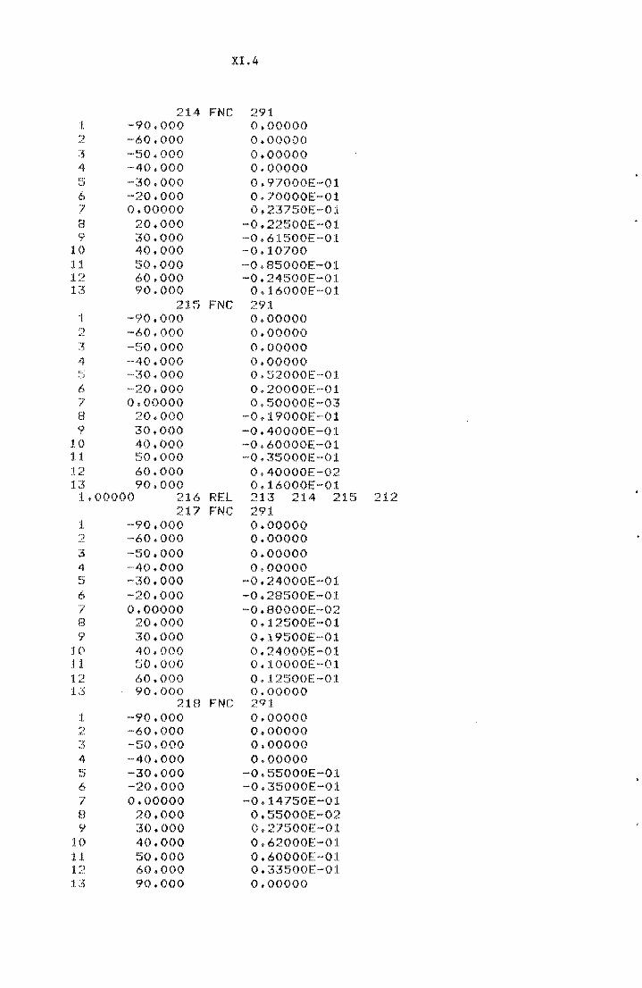
XI. 4
214 FNC 29:1 1 .. ·(to • 000 O.OOOO() r~ '-60.000 0.00000 ......
;3 .-.~j() • 000 O.OO()OO 4 ·-4().000 O.O()()OO ~::; ·-3O.O()() o • 9'70()()E ... ():I. 6 ""20.000 O. lOOOOE --O:l ? o.O()OOO O. ~~:57!:.)OE --O:l 8 20.000 -0. 22~.)OOE--O 1 9 :30.000 -0.6:1. ~')OOE -O:l
:to 40.000 '-0.:1.0700 :1.1 !SO • 000 --0. 85000e>··0 1 :I. ::? 60.0()O '-0 • 24~')()()E: --0:1. 1 ~5 90.000 O. :l6000E --0:1.
21 ~:; FNG 29:L :1 ._<y() • OO() o .OO()OO ") ,," .. '-60.000 O.()()()()() 3 -:::;0 + ()()() O.OO()OO 4 ····40.000 0.00000 C' ,.) ·_·30.0()() O. ~';2000E··-O:l. f) .. ··20.000 0.2()O()OE"-O:l. I' 0.00000 O. ~500()OE--03 El 20.()O() '-0. :l9000E -O:l 9 30.0()O -·0. 40()()OE"-O:t
to 40.()()O '-0. 60000E ... () 1 :t.1 !'':;O • O()O '-0. ;35000E --0:1. :1.2 60.000 0.4()OOOE-02 1.3 90.000 O. :1. 6000E --01
1.()OOOO 216 REL 21:3 214 21. ~.:; 212 2:L7 FNC 291
1 --(to .. 000 0.00000 ~~ '-60.000 0.00000 :~ '-50.000 0.00000 4 --40.000 O.O()OO() c:· ,.J --30.000 --O.24000E-O:l. I.> -<W.OO() -0. 28~.)()OE·-O:l. 7 O.()O()()O -0 .. 80()OOE "-02 8 :W.OOO O. :L 2500E "-01 9 30.0()() 0 .. :l n:;()OE--Ol
10 40.000 O. :?4000E--Ol .1J. ~jO .000 O.:l.OO()OE--O:L 12 6)0.000 O. :I. 2~5()OE --0:1. 1 ~5 90.0()O O.O()()()()
2:1.13 FNC 29:1. :I. -(10.000 O.()O()()() .") .,",. -60.000 0.00000 3 -~.:;O • 000 O.OO()OO 4 --40.000 O.OO()O() c;-,.J --30.000 -0 .. 55000E --O:L 6 "-:W.OOO -0.3500()E--O:L 7 0.00000 --0. :l47!50E-Ol B 20.0()0 () • !::;5()()()E -02 9 30.0()0 o • 27~500E --0:[
:1.0 40.()()O O. 6~?()()OF"·():I. :I. :I. ~;:.;O • 000 0 .. 6 (H) () ()[ .... ():J. 1.2 60.()()O (). 33~H)()E··-O:L :1.3 90.000 0.00000
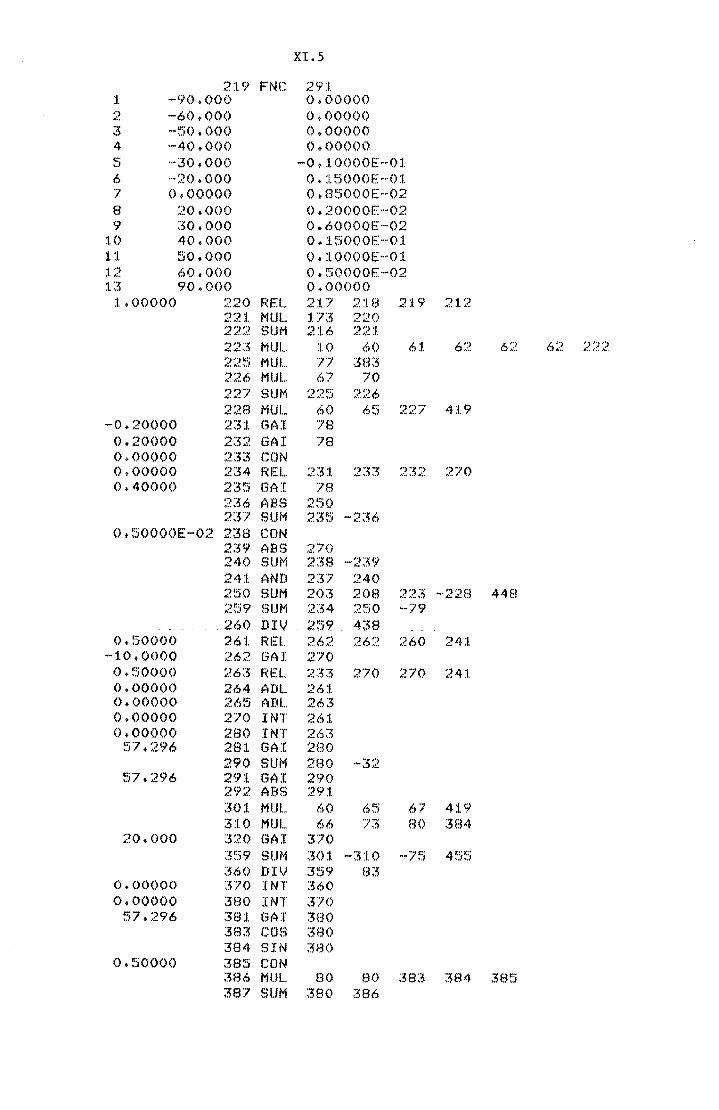
XI.5
219 FNC 291 1 -90.000 0.00000 2 -60.000 0.00000 3 -50.000 0.00000 4 -40.000 0.00000 ~ ~ -30.000 -0.10000E-01 6 -20.000 0.15000E-Ol 7 0.00000 0.85000E-02 8 20.000 0.20000E-02 9 30.000 0.60000E-02
10 40.000 0.!5000E-01 11 50.000 O.IOOOOE-O! 12 60.000 0.50000E-02 13 90.000 0.00000
1.00000 220 REL 217 218 219 212 221 MUL 173 220 222 SUM 216 221 223 MUL 10 60 61 6? - 62 6? h 222 225 MUL 77 383 226 MUL 6'7 70 227 SUM 225 226 228 MUL 60 65 227 419
-0.20000 231 GAl 78 0.20000 232 GAl 78 0.00000 233 CON 0.00000 234 REL 231 233 232 270 0.40000 235 GAl 78
236 ABS 250 237 SUM 235 -236
0.50000E-02 238 CON 239 ABS 270 240 SUM 238 -239 241 AND 237 240 250 SUM 203 208 223 -228 448 259 SUM 234 250 -79 260 DIV 259 438
0.50000 261 REL 262 262 260 241 -10.0000 262 GAl 270 0.50000 263 REL 233 270 270 241 0.00000 264 ADL 261 0.00000 265 ADL 263 0.00000 270 INT 261 0.00000 280 INT 263
57.296 281 GAl 280 290 SUM 280 -32
57.296 291 GAI 290 292 ABS 291 301 MUL 60 65 67 419 310 MUl 66 73 80 384
20.000 320 GAl 370 359 SUM 301 -310 -75 4~r J~
360 DIU 359 83 0.00000 370 INT 360 0.00000 380 INT 370
57.296 381 GAI 380 383 COS 380 384 SIN 380
0.50000 385 CON 386 MUL 80 80 383 384 385 387 SUM 380 386
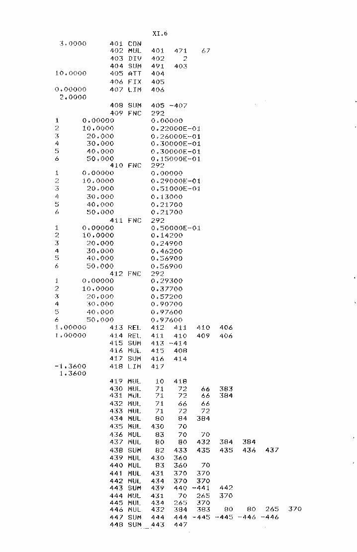
XI.ti
3.0000 401 CON 402 MUL 401 471 67 403 DIV 402 ~ , 4()4 SUM 491 4()3
10.0000 405 ATT 404 4()6 FIX 4()5
0.00000 407 LIM 406 2.0000
408 SUM 405 -407 4()9 FNC 292
1 0.00000 0.00000 ~ , 10.0000 0.22000E-Ol 3 20.000 0.26000E-Ol 4 30.000 0.30000E-Ol ~ J 40.000 0.30000E-Ol 6 50.000 0.15000E-Ol
410 FNC 292 1 0.00000 0.00000 ~ , 10.0000 0.29000E-01 3 20.000 0.51000E-01 4 30.000 0.13000 ~ J 40.000 0.21700 6 50.000 0.21700
411 FNC 292 1 0.00000 0.50000E-Ol 2 10.0000 0.14200 3 20.000 0.24900 4 30.000 0.46200 5 40.000 0.56900 6 50.000 0.56900
412 FNC 292 1 0,00000 0.29300 2 10.0000 0.37700 3 20.000 0.57200 4 30.000 0.90700 5 40.000 0.97600 6 50.000 0.97600 1.00000 413 REL 412 411 410 406 1.00000 414 REL 411 410 409 406
415 SUM 413 -414 416 MUL 415 408 417 SUM 416 414
-1.3600 418 LIM 417 1.3600
419 MUL 10 418 430 MUL 71 72 66 383 431 MUL 71 72 66 384 432 MUL 71 66 66 433 MUL 71 72 72 434 MUL 80 84 384 435 MUL 430 70 436 MUL 83 70 70 437 MUL 80 80 432 384 384 438 SUM 8 7 - 433 435 435 436 437 439 MUL 430 360 440 MUL 83 360 70 441 MUL 431 370 370 442 MUL 434 370 370 443 SUM 439 440 -441 442 444 MUL 431 70 265 370 445 MUL 434 265 370 446 MUL 432 384 383 80 80 265 370 447 SUM 444 444 -445 -445 -446 -446 448 SUM 443 447
XI. 7
~----..
450 MUI ... 430 264 451 MUL 83 '70 ~!64 4~52 MUL 43:L '70 265 26~)
45~~ MUL 80 80 432 ~583 3f.i4 26~; ~~b~)
4~)4 MUL 4;H 26!:) ~?6!:)
455 SUM 450 451 .. -452 4:'::;~5 454 470 SUM 26!:1 -370
57. ~~96 471 GAr 470 480 SUM :?8() --387
57.296 4!H GAl 480 490 SUM 480 -<52
:;7.296 491 GAI 49()
:fI:
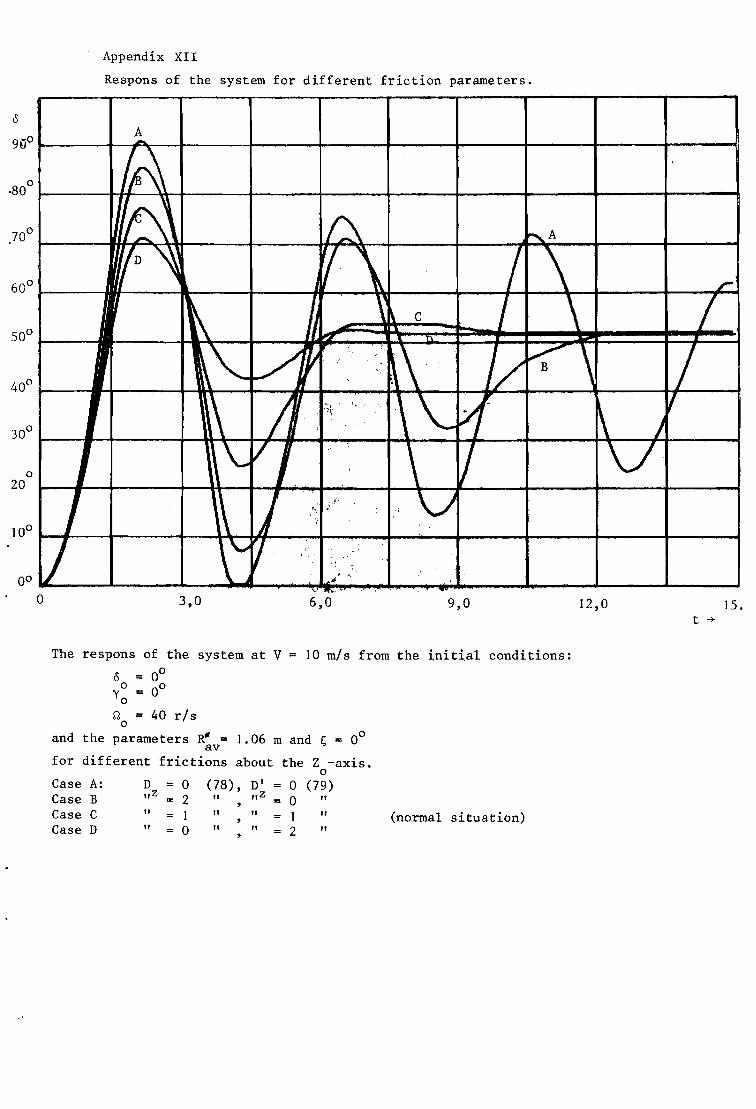
o ·80
o 20
00
Appendix XII
Respons of the system for different friction parameters.
!.
~ ~ 6 ~A
lIn ~ [\ / \ 11/ 1 I \ ~
, C
f ",
.~ ~ :.
~\ I
~\ I J/ 1. --
~\ ;J .'~l t, ',' . \'--~ ~ )
'- Ij \ V V
} ~ j •• : I·;' ' . V .;
,,\
II \~ V " , .' ; , ' ; ~'" ..
-\.., "'-..., ".
o 3,0 6,0 9,0 12,0
The respons of the system at V = 10 mls from the initial conditions:
<5 00
o 00 Yo ~
o 40 rls
and the parameters R* = 1.06 m and ~ = 00
av for different frictions about the Z-axis.
o Case A: D
lIZ = 0
2 1 o
(78), D' lIZ
o (79) Case B Case C Case D
" "
" " "
" "
o 1 2
" " "
(normal situation)
r
/ /
I
15. t -+
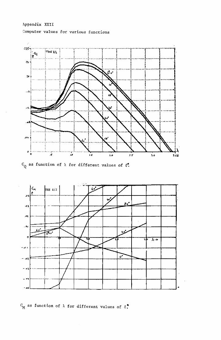
Appendix XIII
Computer values for various functions
,11)'':'"'''''' ": .. '''., .. :., .. , ... 'p'''''''' : ......... 1' ....... ·t··· ...... I· .... •• ... • .. • .. • ... ·········f j .. c.- inHifl/z. :,' ~ ! ! i ! : ! "
-~ ;:: I I : l :t : t : : t t : f ........ . .. • • • ....... ~ ............ ~ ••• ~ •••• : ••• f ..... f····· .. ·· .. ·l······· ... : ......... . :' ....... ":" H" ::..:. i I
·llf 1; ......... : . ::! 1 I i I I .. .~ .. :.... : ... I·····~·········:· .... ······:·········!·········I "-...... 00.:.... .. • '" • : .. ~ • : : t •
C):. 0.. .. ; '" : i I ! I
.. : .......... : ......... : .......... , ....... "., : ! I i I
: t ! . : : I • ... ··!······ .. ··j· .. ·······j·········I' : ; ! . I : I "
.. "' .. " ....... , • "' .. '" "' ....... : ............. & : : I" : i i ! i i ··i .. ·· .. ·····:· .. ·······i : : .
.. '\. i i . . .......... I" ............ '" "'I : ;
! i "': .............. '" 'f' .t)'t 1 i " ........ !
I
l.S' "'.0
CQ as function of A for different values of o~
... , . . .....
uP V C'" trHE 1/2 t -
/ jY B"t --.0"
---'-
o
/ - """ ,...-- / ~ d~
V V
J ~ 't). ~
'" I ~ ~
~ &\,,' I
I' ~l.~ .,., A-+
~ ~- .. ---~-.- -- r--- --......
---7 ~ !=== '--
/ -1 ---'-
7 If f-----V
."'1.
. "I
-." I
-.0
-."
-.0 " /'
CM as function of A for different values of o~
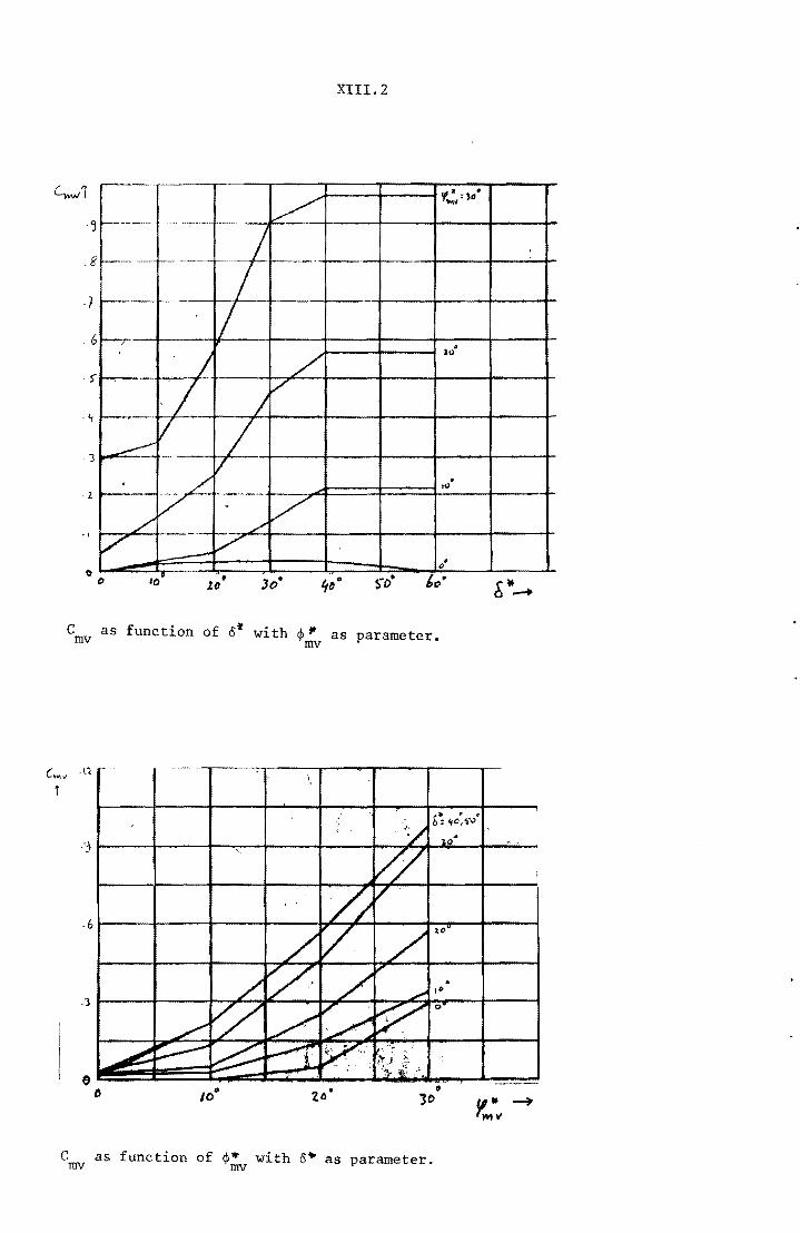
XIII. 2
,.---"
,8
'f:'~; ,,, • V 1--- .. - -" '''' - ~--
/ / -r--'
7 1./ ,
/ / f--,---,
./ J V
1----V 7 ~ -.. v
,6
J
V . ,,,
---/
./ /'"
'/ -- / o· . -. • 10 • I.D so
C as function of c· with ~ It as parameter. mv mv
C as function of ¢. with c~ as parameter. mv mv
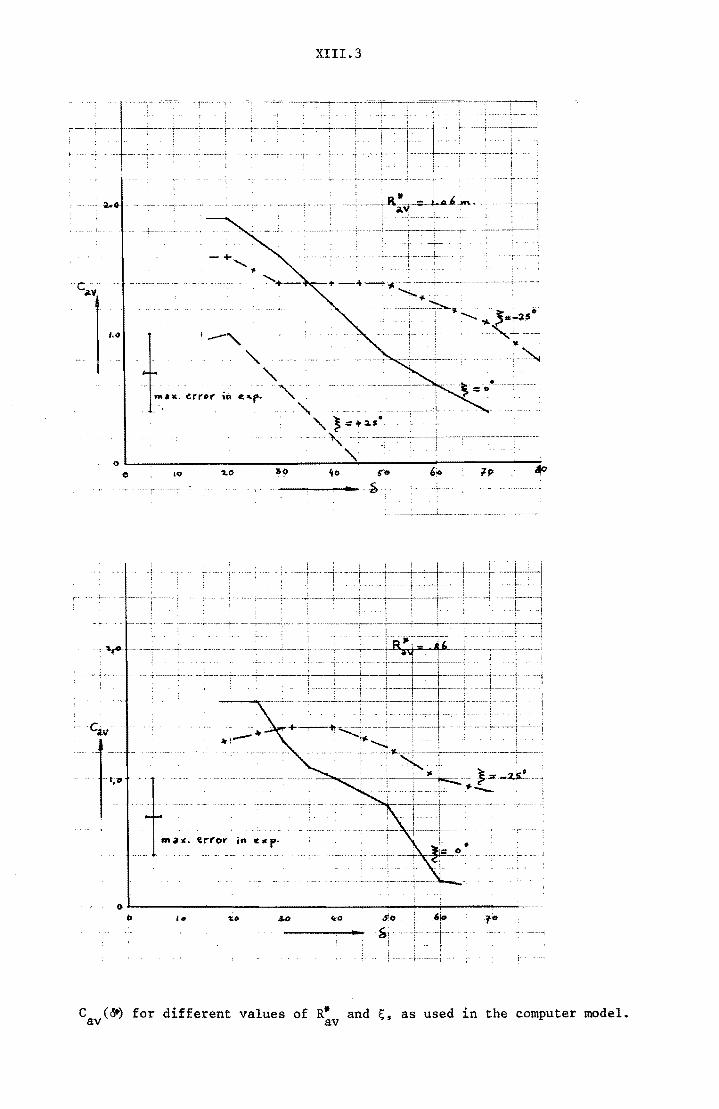
XIII. 3
/.G
l ... <m~:.""~ "~=+2.S. " -------.----.~---.-.-.,.-.--..... ----.-.,---- .. --
"-.~L-~------__ ----------------~~--------~----~----~ e 10 ~I) ""0 '10 ~ ~ --......,.-...,.-... .., .. ~-:--
. -C.iv··
l· errQr in c .. ,.
~~--------------------------------~--~--+-----~--~ Ii» to to 40 ~o ,t;, . -----,.-_ ..... -~.-+-+--
1 ..• r -t--:
c (~) for different values of R* and~, as used in the computer model. av av
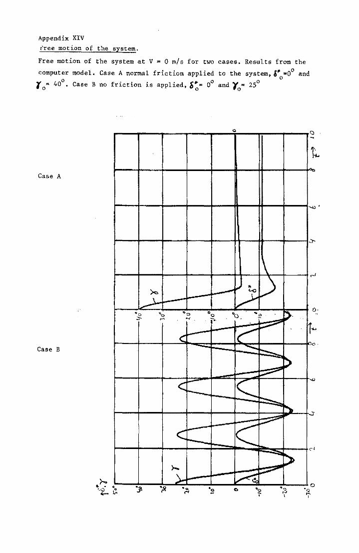
Appendix XIV Free motion of the system.
Free motion of the system at V = 0 mls for two cases. Results from the
computer model. Case A normal friction applied to the system, &~ =0° and ° '10= 40°. Case B no friction is applied, &~= 0° and Yo= 25°
o
Case A
~ l...--" ~ ~
.....-l-1'-'-- ~ <>0 °0 ' '" "0 "0 °0 ;:;;- t"" '" -. .
.,
<: ~ rC Case B ..........
~
~ < ~
r: <: I'-' ~
}o..
)... ,...- K .~
\ l) Q. -~ ~ -
.-!!III
~
~ --....... ~
~
.....
-~
p. ",
>
~. ,...
~
Q, -
-..0
,),-
,....J
0
rr·
'..a
.,J'
<:..f
D '0 1"\ I
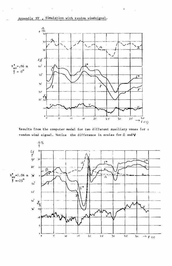
R-av J
Appendix XV , S~ulation with random windsignal •
.n.. f ('/~ ,,0
~--I 'v .... ,
.Jl.
..
OLI ______ L-____ ~~ ___ ~ ____ ~ ______ ~ ____ ~ ____ ~ ____ ~ o .,..
Results from the computer model for two different auxiliary vanes for 11
random wind signal. Notice the difference in scales for..n and V
nr!> f
d/y ~c ---- I f -=-ti\ ~O' Ai) _,_w. -- -~~-
80" 10
,. ./
=1.06 m 10' ()
=-25° r,,;
C:;Ofl ---+---'lI--+--+-+------+-------1r----+-----t-----+-------
. €to V'
1'~ 10' I S\ -~-~.-- --
r
I{) \
5'
o 10 I~ 20 30 ~o --":> t (s)
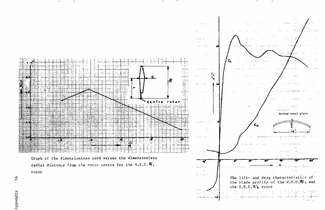
Graph of the dimensionless cord versus the dimensionless
radial dist"lnce from the rotor centre for the T.J.E.U.Df.
rotor
Arched steel plate
lit
The lift- and drag characteristics of the blade profile of the w.E.u.lIft and the T.R.E. Zh. rotor
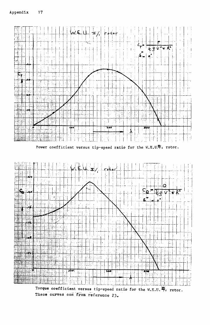
Appendix 17
Power coefficient versus tip-speed ratio for the W.E.U~, rotor.
Torque eoefficie·nt versus tip-speed ratio for the W.E.U.~~ rotor. These curves com from reference 23.
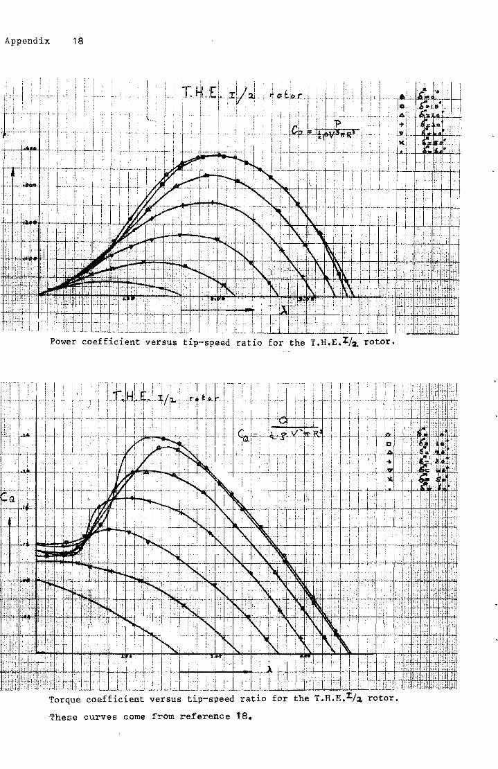
Appendix 18
,[I, i;' I " I~I~ 2.f iii I
• ! ' i ~" c' !'
Power coefficient versus tip-speed ratio for the T.H.E.~/1 rotor.
Torque coefficient versus tip-speed
These curves come from reference f8.
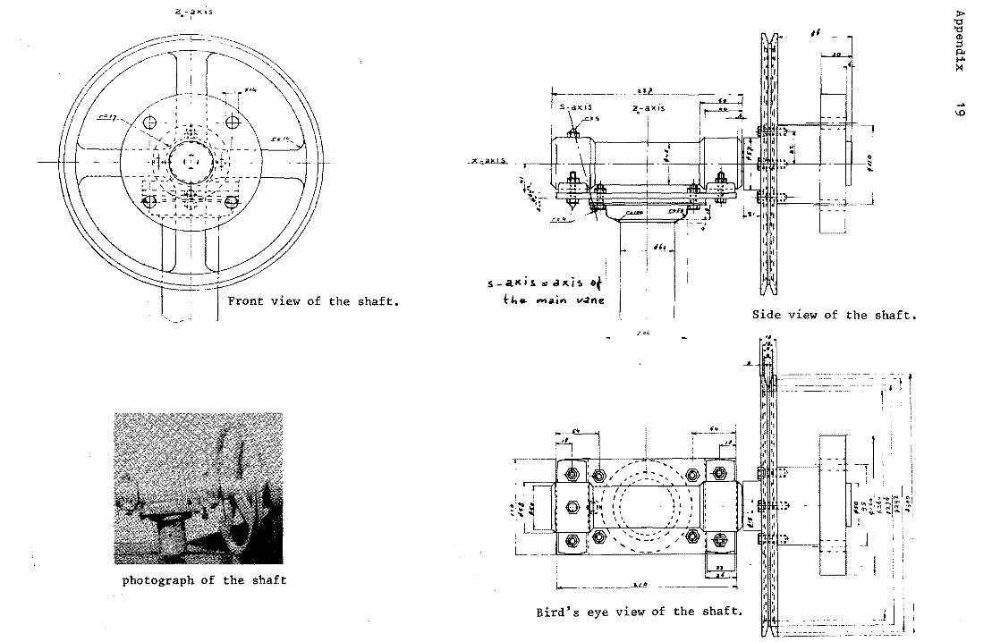
2. -<)>('5 • I
view of the shaft.
photograph of the shaft
s - ax i ~ ::; .a x. i!a of tl. .. _.in v.ane
_.~!l. .. ______ _
2.-ax is
, r:r==?f-~~~~:'/L,~~~~\~,~~1. 1 I,' '. '
. ,
" of' , , I I, \ \ / I I
1---- - ---.--.-.~--------l
Bird's eye view of the shaft.
I I , I I
I
I' , , I, " tt II
1'1 .
Side view of the shaft.
. -, T~l I
, : I . . I I
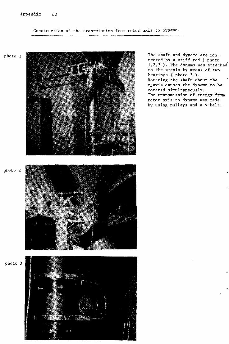
Appendix 20
Construction of the transmission from rotor axis to dynamo.
photo 1
photo 2
photo 3
The shaft and dynamo are connected by a stiff rod ( photo 1,2,3 ). The dynamo was attached' to the z-axis by means of two bearings ( photo 3 ). Rotating the shaft about the z.axis causes the dynamo to be rotated simultaneously. The transmission of energy from rotor axis to dynamo was made by using pulleys and a V-belt.
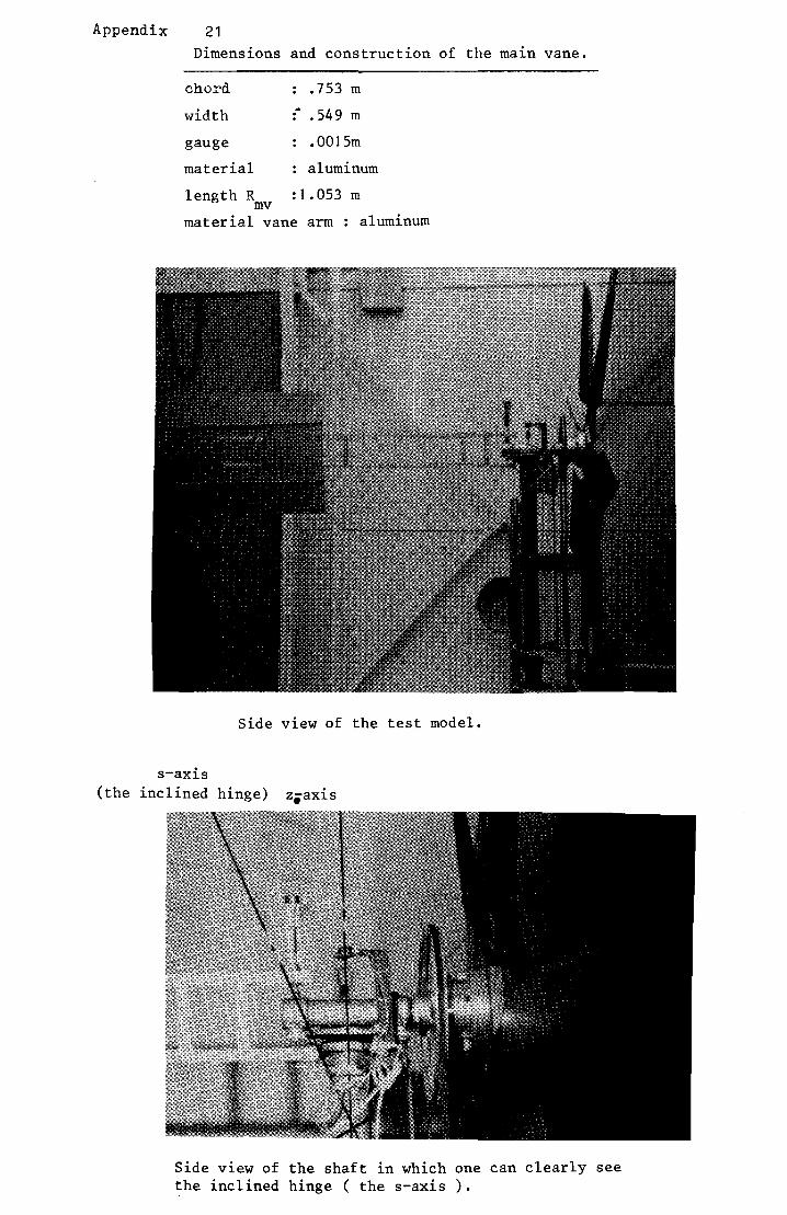
Appendix 21 Dimensions and construction of the main vane •
chord • 753 m
width - .549 m
gauge .00I5m
material aluminum
length R : 1.053 m mv
material vane arm : aluminum
Side view of the test model.
s-axis (the inclined hinge) zoax~s
Side v~ew of the shaft in which one can clearly see the inclined hinge ( the s-axis ).
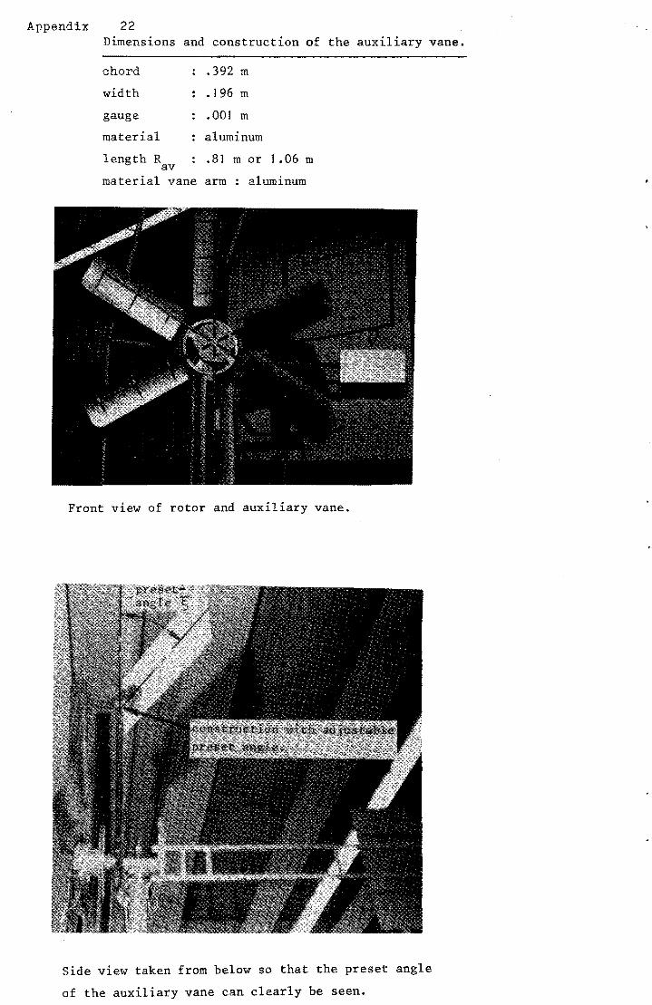
Appendix: 22 Dimensions and construction of the auxiliary vane •
chord . 392 m
width .196 m
gauge .001 m
material aluminum
length R .81 m or 1 .06 m av material vane arm . aluminum .
Front view of rotor and auxiliary vane.
Side view taken from below so that the preset angle
of the auxiliary vane can clearly be seen.
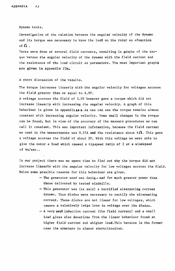
AppenO,l.X ~j
Dynamo tests.
Investigation of the relation between the angular velocity of the dynamo
and its torque was necessary to know the loan on the rotor as afunction
of n . Tests were done at several field currents, resulting in graphs of the tor
que versus the angular velocity of the dynamo with the field current and
the resistance of the load circuit as parameters. The most important graphs
are given in appendix 23a.
A short discussion of the results.
The torque increases linearly with the angular velocity for voltages accross
the field greater than or equal to 4.9V.
A voltage accross the field of 2.0V however gave a torque which did not
increase linearly with increasing the angular velocity. A graph of this
behaviour is given in appendix~la.A~ one can see the torque remains almost
constant with increasing angular velocity. Some small changes in the torque
can be found, but in view of the accuracy of the measure procedures we can
call it constant. This was important information, because the field current
we used in the measurements was O.37A and the resistance about 6fl.. This gave
a voltage accross the field of about 2V. With this voltage we were able to
give the rotor a load which caused a tipspeed ratio of 2 at a windspeed
of 4m/sec ••
In our project there was no spare time to find out why the torque did not
increase linearly with the angular velocity for low voltages accross the field.
Below some possible reasons for this behaviour are given.
- The generator used was desig-ned for much greater power than
those delivered by tested windmills.
- This generator was (as said) a rectified alternating current
dynamo. Thus diodes were necessary to rectify the alternating
current. These diodes are not linear for low voltages, which
causes a relatively large loss in voltage over the diodes.
- A very small induction current (the field current) and a. small
load gives also devations from the linear behaviour found at
higher field current and ahigher load.This because in the former
case the armature is almost shortcircuited.
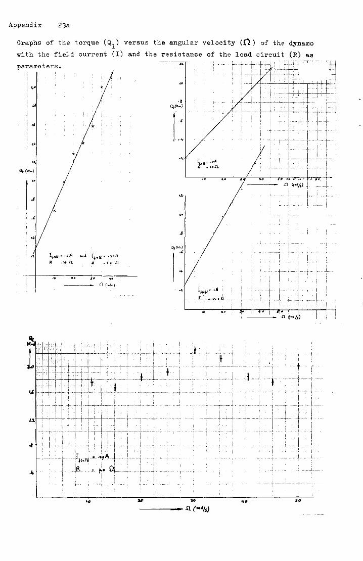
Appendix 23a
Graphs of the torque (Ql) versus the angular velocity «(1) of the dynamo
with the field current (I) and the resistance of the load circuit (R) as
parameters •
..
,(
•• J If,.U' .;o.all ,« < (.1 .n
I.
.8
I~~Il' ,1,4 :
R.,,,,~._ • .si .
l\)
---_ ....... ..Q (t.tA,s)
!
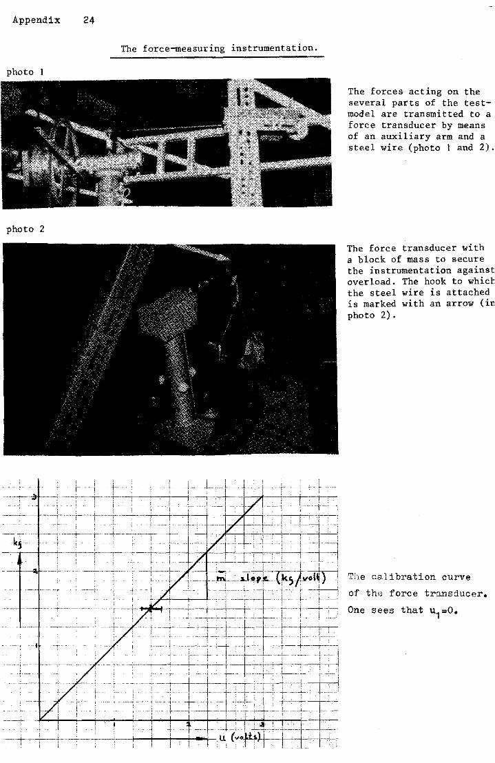
Appendix 24
The force-measuring instrumentation.
photo ]
photo 2
The forces acting on the several parts of the testmodel are transmitted to a force transducer by means of an auxiliary arm and a steel wire (photo I and 2),
The force transducer with a block of mass to secure the instrumentation against overload. The hook to whicb the steel wire is attached is marked with an arrow (in photo 2).
The calibration curve
of the force transducer.
One sees that U 1=O.
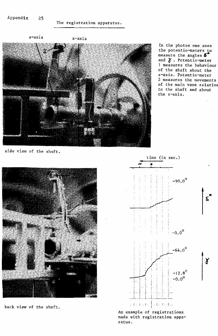
Appendix 25 The registration apparatus.
s-axis z-axis
side view of the shaft.
back view of the shaft.
In the photos one sees the potentio-meters to measure the angles ,and '0 . Potentio-meter 1 measures the behaviour of the shaft about the z-axis. Potentio-meter 2 measures the movements of the main vane relative to the shaft and about the s-axis.
time (in sec.) .. Ie o
. ii' • !
~""':.'.':. . ' . . .
" . ,. . . , .' . • . I •
o -0.0
An example of registrations made with registration apparatus.
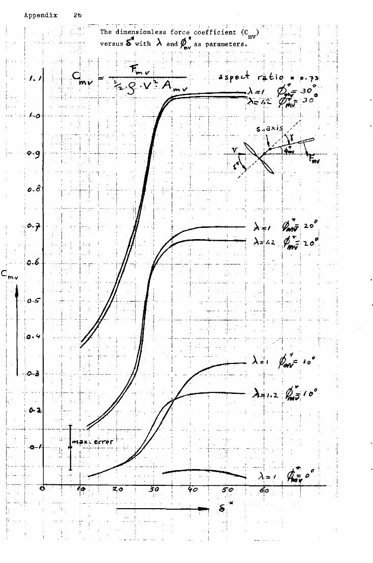
Appendix 2b
'0' . , . . , t"nV
I. I
. <>.;t~ ; I
I " 1 I
';~i !
" i
< t +'T---' i
The dimensionless force coefficient (c ) :If \ ~it mv
versus S with 1\ and as parameters. /,1\(
i j:C
I .. J
~fl A:l!.2. 'I'
t ,
A ~, '1-
A.; 1.2. , ~;.I DD
~1f':.' t1 <; (),
'. .,.
:---i-___ ..:..-~ ____ ....,. Ii. , '1
'"
;.
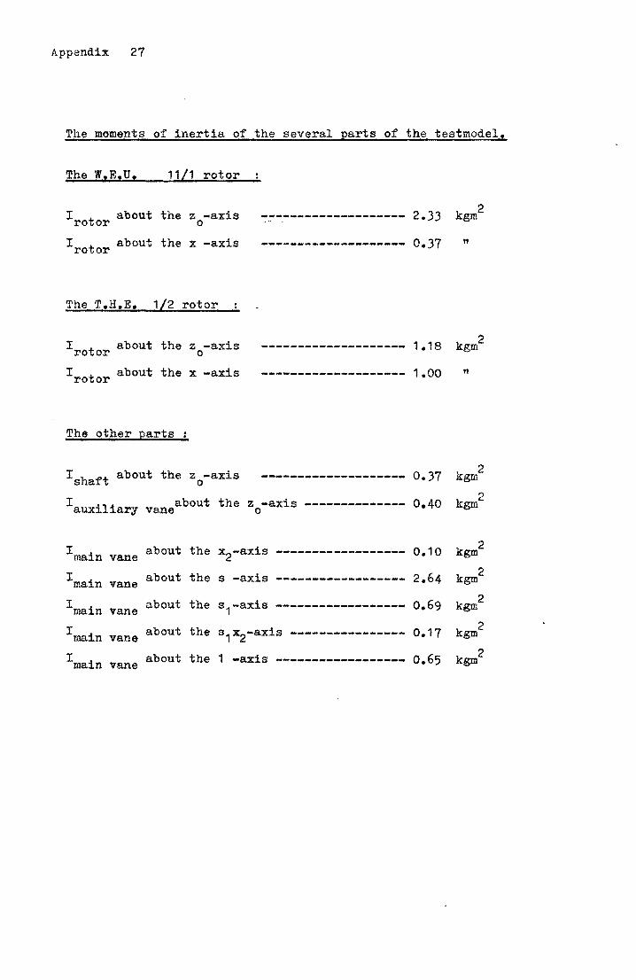
Appendix 27
The moments of inertia of the several parts of the testmodel.
The W,E.U. 11/1 rotor
Irotor about the -axis 2.33 kgm 2 z --------------------0
I about the x -axis -------------------- 0.37 " rotor
The T.H.E. 1/2 rotor
I about the zo-axis 1.18 kgm 2 rotor --------------------
I about the x -axis -------------------- 1.00 " rotor
The other parts
I about the -axis 0.37 kgm 2 shaft z --------------------0
I about the -axis 0.40 kgm 2 auxiliary z --------------vane 0
I about the x2-axis 0.10 kgm 2 main ------------------vane
I about the -axis 2.64 kgm 2 main s ------------------vane
I about the s,-axis 0.69 kgm 2 main ------------------vane
I about the s1x2-axis 0.17 kgm 2 main ----------------vane
I about the 1 -axis 0.65 kgm 2 main ------------------vane
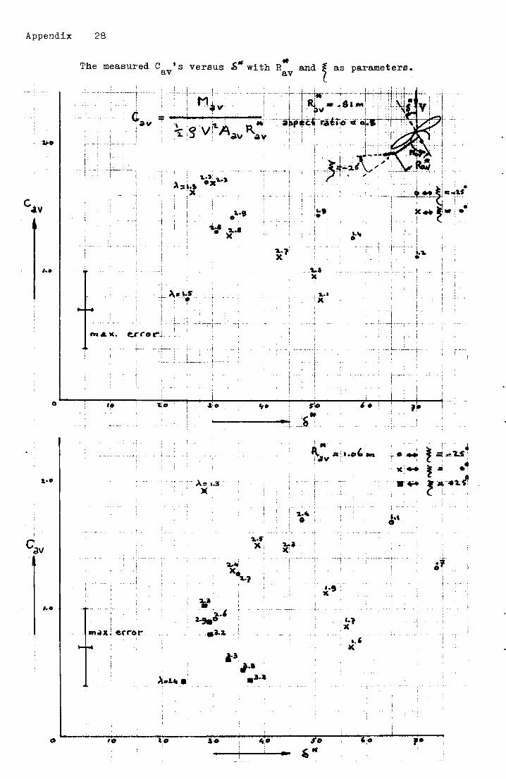
Appendix 28
c.-v
-,..
o
1.-0
The measured C 's versus Sf#. wi th R" av av
i ! -.. ~ -.-+-,,- ... ~-.-"-'t'"' - ,
!
¢.,v = 1 i 1
, i-
! I ot;.·,
...... '2..8 )(
. ,
.... 1' X
.~s X
?ol .- X
._- J
~. sro .. +-------.."J; ,
.,
I •• 1
-,"It
i
i I·
,.
1--- --r "1-
i
,..
o I
j ••
Ll X
I.' ' ~ -
:0
I- .1- -, ..... • i· to,.
I !
: I
---t···-
I
!
!
p. I
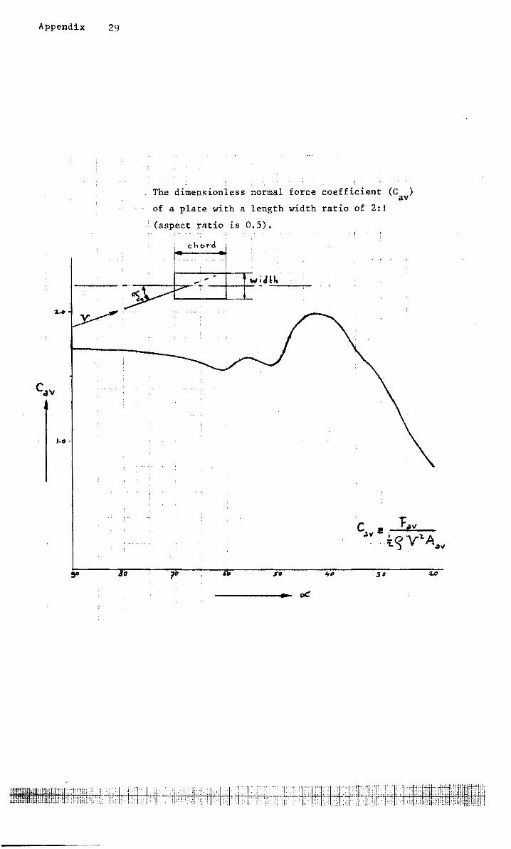
Appendix 29
'.0 .
The dimensionless normal force coefficient (Cav)
of a plate with a length width ratio of 2:1
(aspect r~tio is 0.5).
Ch ord
C J! "F,,, ,W !.o Vl.A
. .. 1..) . /Iv
311
-----....... _ ot:
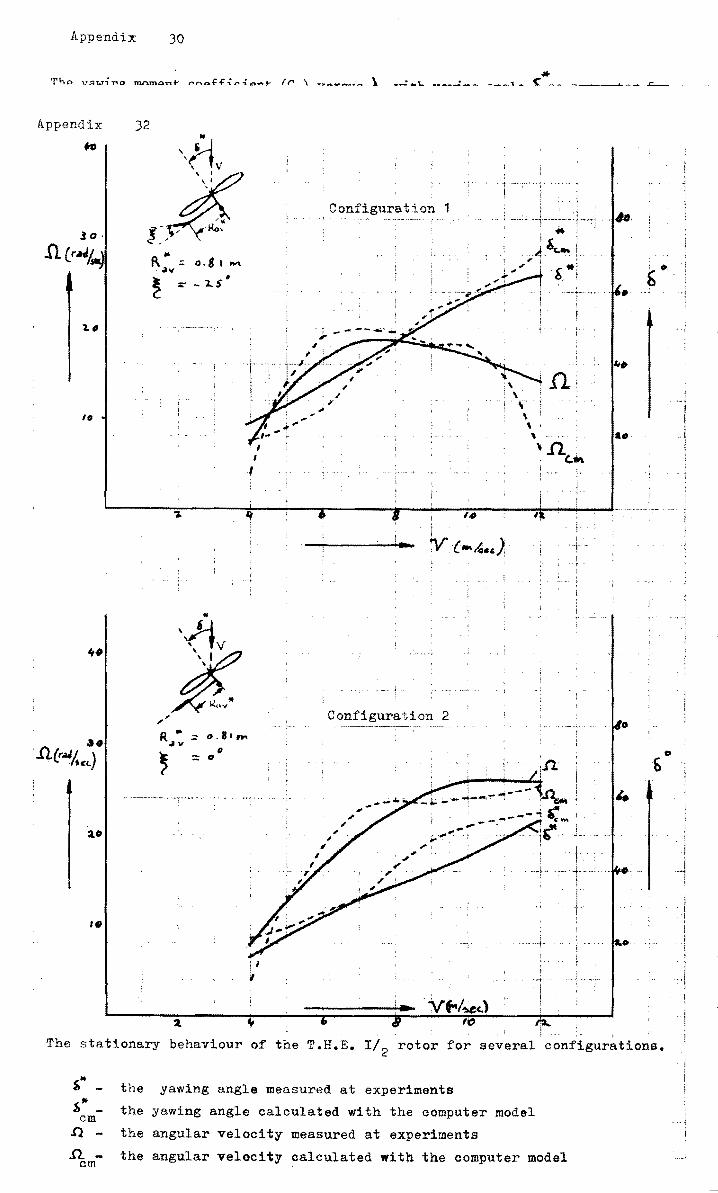
Appendix 30
Appendix 32
fo \ ,~ , .
~\!V
/" ~~, / -Rov
I.
+-
,.
0.' I ......
0.81"" II
:::: "
i I I
----, - _~ __ ~ __ . .1::....-
Configuration 1
'\ :\ . \'
. ~~
\ \ . \ ••
, 1l(..~ I
Configuration 2
I.,
The stationary behaviour of the T.H.E. I/2 rotor for several configurations.
1," _ the yawing angle measured at experiments ~,. -em the yawing angle calculated with the computer model
.Q - the angular velocity measured at experiments
.Q-em the angular velocity calculated with the computer model
i . i
·1 I 1 I i I
I I
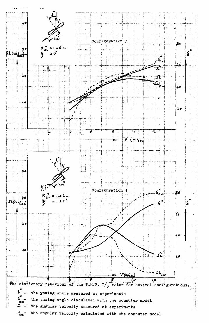
I I· i-'"---- ---I
. , i ' I
1-1 t '. +. i
'I I
r i
.. ~
t , ".: i ., ·.1 . ,
!'V- f.;r-/$ ~. i i '"f
:1 ' ..l
Configuration 4
i i
, ., - I .. , •... _,. 1 , ii' 'Ie' . Ii.,. J .
of-the Tefl.E. 'I!2---rotor for severai1conflgurations. The stationary behaviour
~. -~-em n.n _
em
the yawing angle measured at experiments
the yawing angle claoulated with the oomputer model
the angular velocity measured at experiments
the angular velocity calculated with the computer model
-··1
·,..;
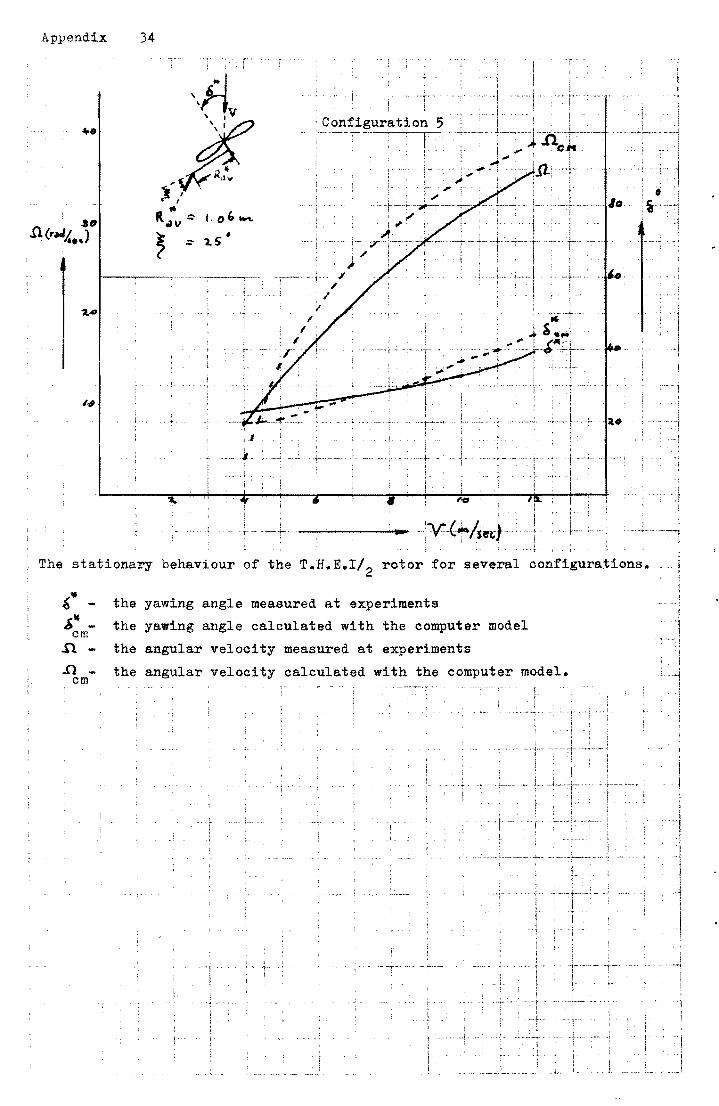
Appendix 34
I,
I I
!Configuration 5
-·i ,
1 i ;. : I
--'----1 ... _ ,;V'·'(t'/Sflc;t-'··,, t
The stationary behaviour of the T.H.E.r!2 rotor for several configurations.
t:* - the yawing angle measured at experiments /,"" - the yawing em angle calculated with the computer model
.n - the angular velocity measured at experiments
.n - the angular em velocity calculated with the computer model.
, .. i
1 ~I
j
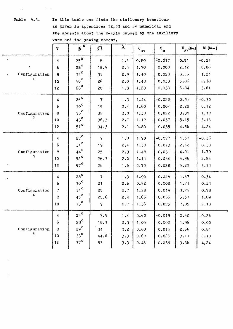
Table 5.3.
.
. Configuration 1
Configuration 2
Configuration 3
,
.
Configuration 4
Configuration 5
In this table one finds the stationary behaviour
as given in appendices 32,33 and 34 numerical and
the moments about the z-axis caused by the auxiliary
vane and the yawing moment.
V Slto .n A C C av m
4 25° 8 1.5 0.80 ':0.017
6 28° 18.5 2.3 1.70 0.000
a 33° 31 2.9 1.40 0.023
10 50° 26 2.0 1.48 0.033
12 66° 20 1.3 1.20 0.030
4 26° 7 1.3 1.44 -0.022
6 30° 19 2.4 1.60 0.004
8 33° 32 3.0 1.30 0.022
10 43 0 36.3 2.7 1 .12 0.037
12 51° 34.3 2.1 0.80 0.035
4 27° 7 1.3 1.90 -0.027
6 34° 19 2.4 1.30 0.013
8 44° 2,5 2.3 1.48 0.031
10 52° 26.3 2.0 1.13 0.034
12 57° 26 1.6 0.70 0.028
4 28° 7 1.3 1.90 -0.025
6 30° 21 2.6 0.92 0.008
7 34° 25 2.7 1.28 0.019
8 45° 25.6 2.4 1.66 0.035
10 73° 9 0.7 1.36 0.025
4 25° 7.5 1.4 0.60 -0.019
6 28° 18.3 2.3 1.05 0.000
8 29° 34 3.2 0.80 0.015
10 330
44.6 3.3 0.60 0.025
12 37° 53 3.3 0.45 0.035
M av(N ... ) M (N ... )
0.51 -0.24
2.42 0.00
3. '>5 1.24
5.86 2.78
6.84 3.64
0.91 -0.30
2.28 0.12
3.}0 1.18
5.15 3.16
4.56 4.24
1.57 -0.36
2.42 0.38
4.91 1.70
5.86 2.86
5.22 3.33
1.57 -0.34
1.71 0.23
3.25 0.78
5.51 1.89
7.05 2.10
0.50 -0.26
1.96 0.00
2.66 0.81
3.11 2.10
3.36 4.24
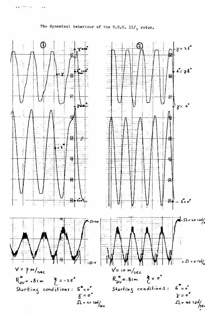
The dynamical behaviour of the W.E.U. III, rotor.
1
L-~l---t-----i-+ --f----jf-- +~++-!I::oH--+--+-
\
'"
-----l~ -- r - i
V::: T M/I)8.<-
r:t..;v =- • g I ~ t = - 'Z. 5'0
S.f: ... H"-tin5 cOlAd'r.tiOM.$: ~*=o# .. 0=" .n c 4' l.w./
/{e,
- - -- 1----
- . -- I--R-\j f-- --I---c - U -- tJ \.
---11
r ---
---- ----- -- -r- ;-- -
--. _. ~- --- ---
---- . 1-- -.~~ -- I -- ---- - 1--- I r
~- - --- J - t-- - - - '--- r---
(j
.-- -.-.- - -. -. --. - -1- c_
- -.-.
- ---~--!--I ----- ! ~
j "q -- - -- -.- f-- --. ---+------ --+-- -- ----------
~- - -- -- --------._- ---~-
- -- f--- ---- ----._-- ----
---.- f- -----.
~-
1
-- -1- --
--
~-t \J -~--- -1--
'1= '" ~!'ec. R.. * :::; . Sf "" ~ ::::: CO ~v c..
5.f:..artik5 CO~J,tl·4III\..s·
0 r:: 0
... . .& ::: ('>
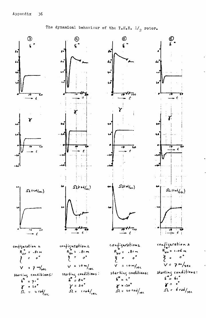
cOlltiSllr.t.o" l. ("O"f i 5 .... r d-ti ()IA. 2-.. w R.lV
::: .81 .... R.a,v :: .81 I'!o\
l ., t ::: 0° :: ()
V ::: t -4c(. V = I (J .,.,/
)4i!<.
St.ari-i .. s (.G ... ~:"io",S: ~tdr{-i ... ) /:o .... Jai(') .. ,s : ,"It "
fit
;:: l' l. = 81.,((1
r .,
Y= 30 • .. :til
.!L =: ... rdJ./. ..Q::: 1".'/ Jee. ~cc..
.r---~ ....... ~I-:IJO -.!... C
(..o .... t' ~1U"t:l ~io .... l. ".w := • &1 """
(I
~ '= ()
" ;:: \ 0-1 ,ee.
si~di~~ ('tJkJWO"&;
," IJ :; 4 I> r .: -:),
£J..::: 40 r'iJ.J! 7~C.
" ·"t--"'!i1-..... ~
!. ;-t-f:
Gc/l\.{~~fArd·i III If\. ..1
RoW': '_e' ...... ~
II .... 0
V= 1- """/-;'Ct! .s+ clt't i ... 5 co ... J,llolll' :
£-M;::. ,.0 0 r= I)
.(l= 6 r.lJI ')C,L
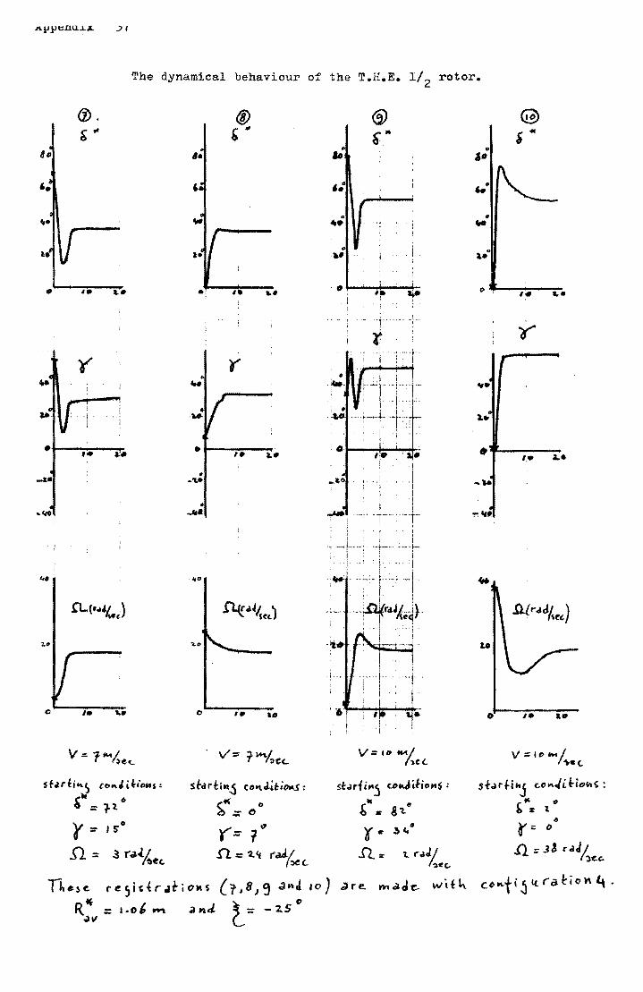
A,tI,tItlLlU.1.Jl ;>1
The
(j). &'"
ID
I. ~.
Y
I I
,,<It
.. If 0
, , ,
4.
.Cl..(, .. d4.J
1."
dynamical behaviour of
(j) , '" 8-
a.
• I. .. it
y • ...
• ,. ... • ..... • .....
~"
~.~1. ) St"
.....
" ,. 110
. V= t~,(..
st~d:h'...s CO"1.li.t;o.o.s:
$,'11(:: () 0
('= 1 .,
n.: ~~ rGJ!/ /,eL
the T.H.E. 1/2 rotor.
® &-
.. ". i I
' .. I I
'. I • zt· , i I
I'
i'" -I
·1, '1· -j I
" ·iw·
,0
" i ,I ... ,,0 "
I I I I
~ : '-t--, I I I
::._.j-
, .. ;''to --t'-"!1~"""~ "
I
sf:.uH"J u ..... i.fioMS:
&tc .. 81."
r '" 3«.·
n. It' 1.. r.J./ 1".)(1(,.
@ , .. " ,.
,." ..
".
I. t..
y-
",.
'1.. • .-
• 1,# ~.
... ...
".., .. "
w
!l.(r-odA ) ~t,
to
o 10
S!drHIIJ (,(J",JH-ilJlk~:
t"z l"
a--:: () .,
..Q;:-.3& C'dell { 'Jt:.c.
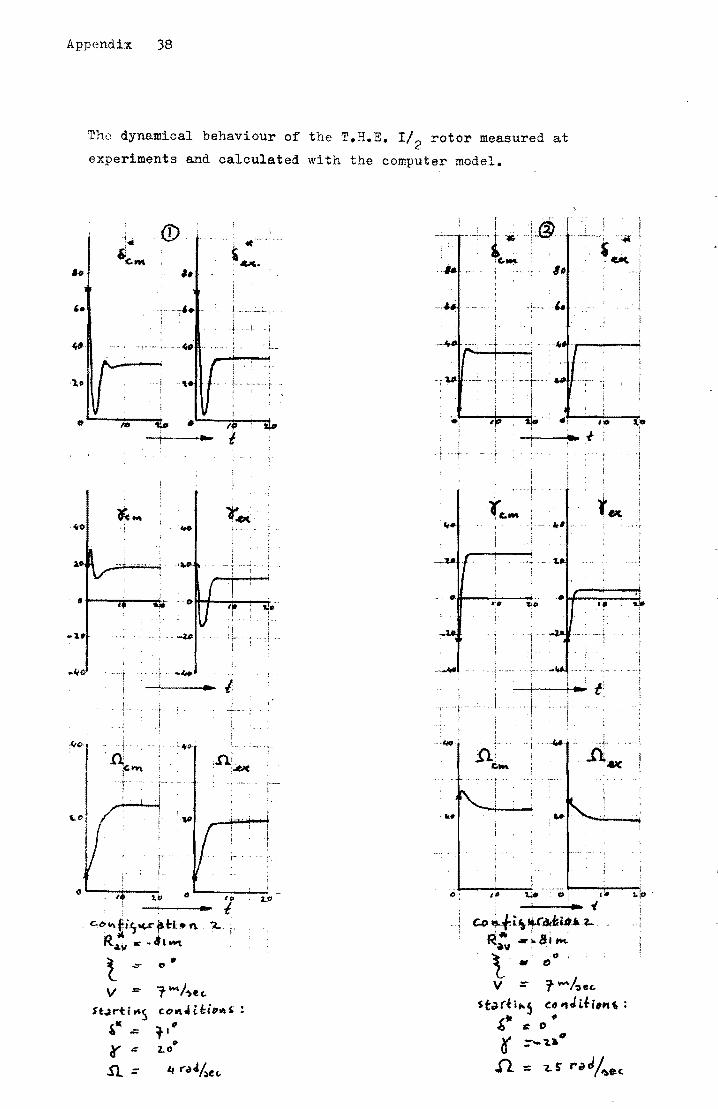
Appendix 38
Tho dynamical behaviour of the T.H.E. I/2 rotor measured at
experiments and calculated with the computer model.
,~,
o--~~-~
...
oj) ., 0' U '. ~o _. t c.,.e>1I\ ~;'t(.r ;.t:-h ~ 4,"
R! ... ';lOOO\
t .::- o·
V ::: l' ""'/-;ftc.
St.:lrth',s ('.0111..( tH,,~s ,- 1·" -= r- .= " 2.0
.n :;- 4 r.,Jher..
'" , ·1
"L -l !
"'1
I' 'I..i_
N,
I I ..II, , ... L
-4 I
0: I
i .. CQ ~fi\t+Idtti.cn2-
'. I : ' R~" ... ~81_
l ell - t)
V :;- T -/~.c. stcl(~it'5 co "Jtfi,"" :
~. :: ..
0
r :=--1.. "
.n. :: ~$' raJ./-:.ec.
, .. ,
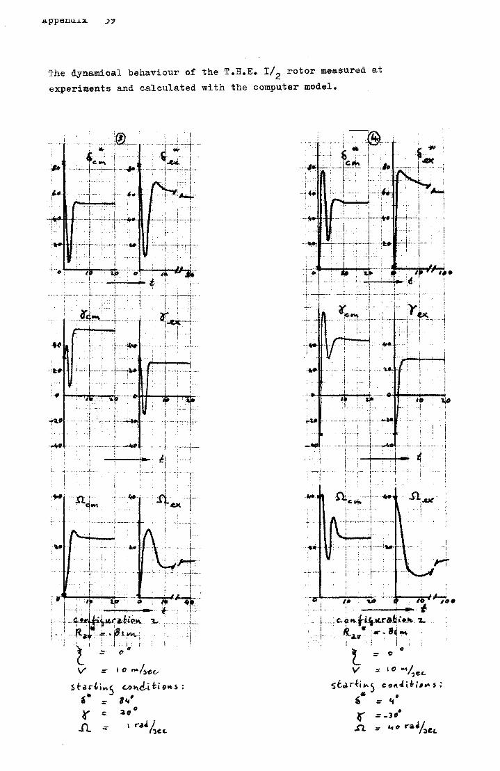
'I'he dynamical behaviour of the T .H.E. I/2 rotor measured at
experiments and calculated with the computer model.
",. I :
I , "I
'-', ---,',1-' I ; ;' I ::
, ar;.U~T' , " 'L.J
-t---!otI""""-- 'il ' ! . "",' 'I"
I ! I
i r "" '~'I'
I
',4~
" ,,'. ~ ,
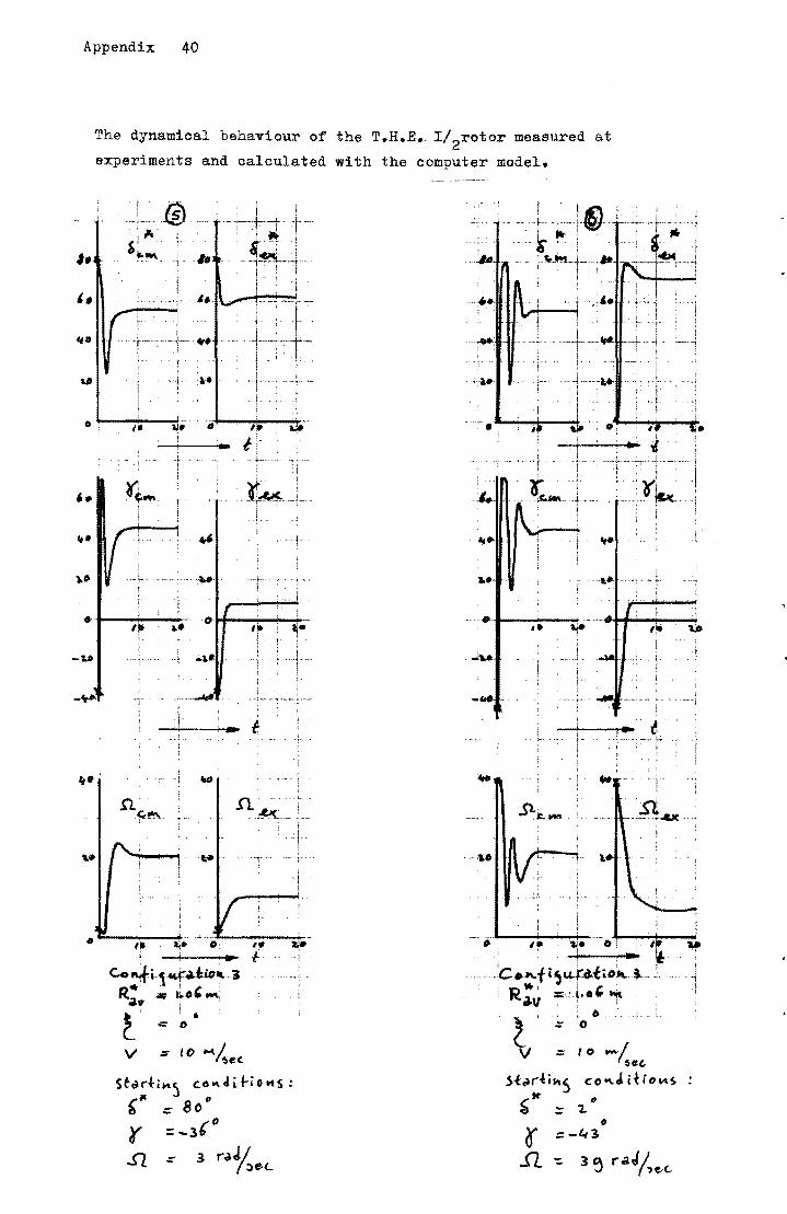
Appendix 40
The dynamical behaviour of the T.H.E •. I/2rotor measured at
experiments and calculated with the computer model.
,.
If.
l_
L , -.,... I .. -4tfI
-+-1--+....... t
".'
.,1;;... ____ +: ID .,. 0 ~.
, ! • f Co ~l-,.....r.I.ao"'~ R:. «; ~o'-;
t coO
V ... it> M~ec.
StpC"'fi"'5 c,c>","iHfHIS:
," -= 80 IJ
r SJ.
= _3(0
--!-,--rtl ...... · t f· ",,",:.----+
, I ! ,
, .1
!
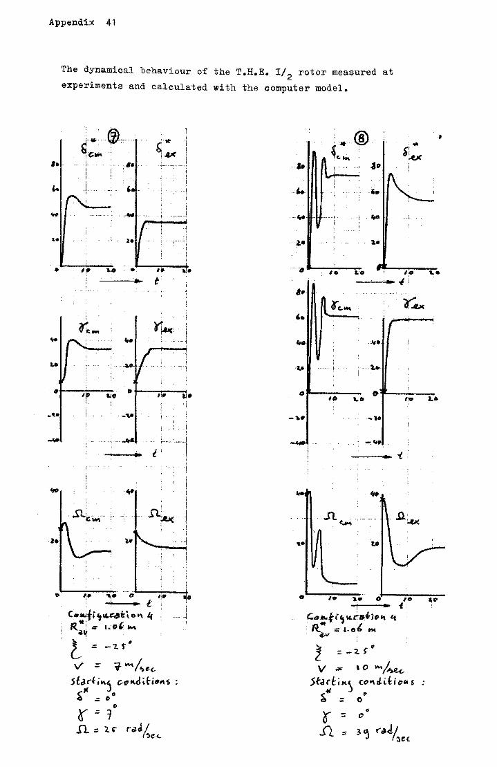
Appendix 41
The dynamical behaviour of the T.H.E. I/2 rotor measured at
experiments and calculated with the computer model.
I.
'" W
iL.
0;
".
1.0
#I
_ ....
-¥'
•
Q-,*"@:T ''It , ' i I & iC"'" 1 . i .tJ(
. j ..... I 1 ,.
·1
I~ I.. .. t
I
~'"
.. ........
.j ... ..If_ , ... i 1
110 "i. "'6 'i. i .. l'
C·::fi.,.~~,o", " R .. ~. t.o' 1001;
L . :::: -"2.. r"'
V =- i- "'" ~e," .stcU~i"'j c.-"",d~H""s
("til 0 ~ ,;: 0
1:1 r ;: '1 n :: 1.. r~J /
I-;'e<..
,I
j • J
,
~o , '1
o
: ® , .... "'" t .. b~ ... , .
·k
-.,. ",. _.1
·-i.e 1.-
.-~ I. &,'. I. ... -I ,I , .
¥'".&Jc '-
4ttt ."", •. .... .2..
0 (I
'P a..o I:.
-1.0 · .. \6
-A.III> .. ... If.
- -t ,
--~-- .. o I'. t;o O. , • .; .. .,:
Co:-fl\ILt.'B:'jO", "t
: f{ ':: '-6' tI4. . ...,. Z =_'2.$"11
V .;;;: to .... /~ .5t<UtiM.) c(')f\.tifi (')", s
<C oft " c :::; 0
o :: ..n.:::
fi
t.a
~.


![[Owen] Mechanical Behaviour of the](https://img.pdfslide.us/doc/110x75/577cd7161a28ab9e789e04ab/owen-mechanical-behaviour-of-the.jpg)