Static Analysis and Veri cation of Aerospace Software by

Static Analysis and Verification of Aerospace Software

by Abstract Interpretation

Julien Bertrane∗

Ecole normale superieure, Paris

Patrick Cousot∗,∗∗

Courant Institute of Mathematical Sciences, NYU, New York & Ecole normale superieure, Paris

Radhia Cousot∗

Ecole normale superieure & CNRS, Paris

Jerome Feret∗

Ecole normale superieure & INRIA, Paris

Laurent Mauborgne∗,‡

Ecole normale superieure, Paris & IMDEA Software, Madrid

Antoine Mine∗

Ecole normale superieure & CNRS, Paris

Xavier Rival∗

Ecole normale superieure & INRIA, Paris

We discuss the principles of static analysis by abstract interpretation and report onthe automatic verification of the absence of runtime errors in large embedded aerospacesoftware by static analysis based on abstract interpretation. The first industrial applicationsconcerned synchronous control/command software in open loop. Recent advances considerimperfectly synchronous, parallel programs, and target code validation as well. Futureresearch directions on abstract interpretation are also discussed in the context of aerospacesoftware.

Nomenclature

S program statesCJtKI collecting semanticsFP prefix trace transformerFι interval transformerV set of all program variablest? reflexive transitive closure

of relation t

lfp⊆F least fixpoint of F for ⊆|x| absolute value of xq quaternionN naturals

I initial statesT JtKI trace semanticsRJtKI reachability semantics

1S identity on S (also t0)x program variabletn powers of relation t

α abstraction function`

widening

X] abstract counterpart of Xq conjugate of quaternion q

Z integers

t state transitionPJtKI prefix trace semanticsFR reachability transformert ◦ r composition of relations

t and r

ρ reductionγ concretization functiona

narrowing℘(S) parts of set S (also 2S)||q|| norm of quaternion q

R reals

∗Ecole normale superieure, Departement d’informatique, 45 rue d’Ulm, 75230 Paris cedex 05, [email protected].∗∗Courant Institute of Mathematical Sciences, New York University, 251 Mercer Street New York, N.Y. 10012-1185,

u.to @ n u esu . yso dccp .‡Fundacion IMDEA Software, Facultad de Informatica (UPM), Campus Montegancedo, 28660-Boadilla del Monte, Madrid,

Spain.

1 of 38

American Institute of Aeronautics and Astronautics

I. Introduction

The validation of software checks informally (e.g., by code reviews or tests) the conformance of thesoftware executions to a specification. More rigorously, the verification of software proves formally the con-formance of the software semantics (that is, the set of all possible executions in all possible environments) to aspecification. It is of course difficult to design a sound semantics, to get a rigorous description of all executionenvironments, to derive an automatically exploitable specification from informal natural language require-ments, and to completely automatize the formal conformance proof (which is undecidable). In model-baseddesign, the software is often generated automatically from the model so that the certification of the softwarerequires the validation or verification of the model plus that of the translation into an executable software(through compiler verification or translation validation). Moreover, the model is often considered to be thespecification, so there is no specification of the specification, hence no other possible conformance check.These difficulties show that fully automatic rigorous verification of complex software is very challenging andperfection is impossible.

We present abstract interpretation1 and show how its principles can be successfully applied to cope withthe above-mentioned difficulties inherent to formal verification.

• First, semantics and execution environments can be precisely formalized at different levels of abstraction,so as to correspond to a pertinent level of description as required for the formal verification.

• Second, semantics and execution environments can be over-approximated, since it is always sound toconsider, in the verification process, more executions and environments than actually occurring in realexecutions of the software. It is crucial for soundness, however, to never omit any of them, even rareevents. For example, floating-point operations incur rounding (to nearest, towards 0, plus or minusinfinity) and, in the absence of precise knowledge of the execution environment, one must consider theworst case for each float operation. Another example is inputs, like voltages, that can be overestimatedby the maximum capacity of the hardware register containing the value (anyway, a well-designed softwareshould be defensive, i.e., have appropriate protections to cope with erroneous or failing sensors and beprepared to accept any value from the register).

• In the absence of an explicit formal specification or to avoid the additional cost of translating the spec-ification into a format understandable by the verification tool, one can consider implicit specifications.For example, memory leaks, buffer overruns, undesired modulo in integer arithmetics, float overflows,data-races, deadlocks, live-locks, etc. are all frequent symptoms of software bugs, which absence can beeasily incorporated as a valid but incomplete specification in a verification tool, maybe using user-definedparameters to choose among several plausible alternatives.

• Because of undecidability issues (which makes fully automatic proofs ultimately impossible on all pro-grams) and the desire not to rely on end-user interactive help (which can be lengthy, or even intractable),abstract interpretation makes an intensive use of the idea of abstraction, either to restrict the propertiesto be considered (which introduces the possibility to have efficient computer representations and algo-rithms to manipulate them) or to approximate the solutions of the equations involved in the definitionof the abstract semantics. Thus, proofs can be automated in a way that is always sound but may beimprecise, so that some questions about the program behaviors and the conformance to the specificationcannot be definitely answered neither affirmatively nor negatively. So, for soundness, an alarm will beraise which may be false. Intensive research work is done to discover appropriate abstractions eliminatingthis uncertainty about false alarms for domain-specific applications.

We report on the successful cost-effective application of abstract interpretation to the verification of theabsence of runtime errors in aerospace control software by the Astree static analyzer,2 illustrated first bythe verification of the fly-by-wire primary software of commercial airplanes3 and then by the validation ofthe Monitoring and Safing Unit (MSU) of the Jules Vernes ATV docking software.4

We discuss on-going extensions to imperfectly synchronous software, parallel software, and target codevalidation, and conclude with more prospective goals for rigorously verifying and validating aerospace soft-ware.

2 of 38


Contents

I Introduction 2

II Theoretical Background on Abstract Interpretation 4II.A Semantics . . . . . . . . . . . . . . . . . . . . . . . . . . . . . . . . . . . . . . . . . . . . . 4II.B Collecting semantics . . . . . . . . . . . . . . . . . . . . . . . . . . . . . . . . . . . . . . . 5II.C Fixpoint semantics . . . . . . . . . . . . . . . . . . . . . . . . . . . . . . . . . . . . . . . . 5II.D Abstraction . . . . . . . . . . . . . . . . . . . . . . . . . . . . . . . . . . . . . . . . . . . . 5II.E Concretization . . . . . . . . . . . . . . . . . . . . . . . . . . . . . . . . . . . . . . . . . . 6II.F Galois connections . . . . . . . . . . . . . . . . . . . . . . . . . . . . . . . . . . . . . . . . 6II.G The lattice of abstractions . . . . . . . . . . . . . . . . . . . . . . . . . . . . . . . . . . . . 7II.H Sound (and complete) abstract semantics . . . . . . . . . . . . . . . . . . . . . . . . . . . 7II.I Abstract transformers . . . . . . . . . . . . . . . . . . . . . . . . . . . . . . . . . . . . . . 7II.J Sound abstract fixpoint semantics . . . . . . . . . . . . . . . . . . . . . . . . . . . . . . . 7II.K Sound and complete abstract fixpoints semantics . . . . . . . . . . . . . . . . . . . . . . . 7II.L Example of finite abstraction: model-checking . . . . . . . . . . . . . . . . . . . . . . . . . 8II.M Example of infinite abstraction: interval abstraction . . . . . . . . . . . . . . . . . . . . . 8II.N Abstract domains and functions . . . . . . . . . . . . . . . . . . . . . . . . . . . . . . . . 8II.O Convergence acceleration by extrapolation . . . . . . . . . . . . . . . . . . . . . . . . . . . 9

II.O.1 Widening . . . . . . . . . . . . . . . . . . . . . . . . . . . . . . . . . . . . . . . 9II.O.2 Narrowing . . . . . . . . . . . . . . . . . . . . . . . . . . . . . . . . . . . . . . . 9

II.P Combination of abstract domains . . . . . . . . . . . . . . . . . . . . . . . . . . . . . . . . 10II.Q Partitioning abstractions . . . . . . . . . . . . . . . . . . . . . . . . . . . . . . . . . . . . 11II.R Static analysis . . . . . . . . . . . . . . . . . . . . . . . . . . . . . . . . . . . . . . . . . . 11II.S Abstract specifications . . . . . . . . . . . . . . . . . . . . . . . . . . . . . . . . . . . . . . 11II.T Verification . . . . . . . . . . . . . . . . . . . . . . . . . . . . . . . . . . . . . . . . . . . . 11II.U Verification in the abstract . . . . . . . . . . . . . . . . . . . . . . . . . . . . . . . . . . . 12

III Verification of Synchronous Control/Command Programs 12III.A Subset of C analyzed . . . . . . . . . . . . . . . . . . . . . . . . . . . . . . . . . . . . . . . 12III.B Operational semantics of C . . . . . . . . . . . . . . . . . . . . . . . . . . . . . . . . . . . 12III.C Flow- and context-sensitive abstractions . . . . . . . . . . . . . . . . . . . . . . . . . . . . 13III.D Hierarchy of parameterized abstractions . . . . . . . . . . . . . . . . . . . . . . . . . . . . 13III.E Trace abstraction . . . . . . . . . . . . . . . . . . . . . . . . . . . . . . . . . . . . . . . . . 14III.F Memory abstraction . . . . . . . . . . . . . . . . . . . . . . . . . . . . . . . . . . . . . . . 15III.G Pointer abstraction . . . . . . . . . . . . . . . . . . . . . . . . . . . . . . . . . . . . . . . . 16III.H General-purpose numerical abstractions . . . . . . . . . . . . . . . . . . . . . . . . . . . . 16

III.H.1 Intervals . . . . . . . . . . . . . . . . . . . . . . . . . . . . . . . . . . . . . . . . 17III.H.2 Abstraction of floating-point computations . . . . . . . . . . . . . . . . . . . . . 17III.H.3 Octagons . . . . . . . . . . . . . . . . . . . . . . . . . . . . . . . . . . . . . . . . 18III.H.4 Decision trees . . . . . . . . . . . . . . . . . . . . . . . . . . . . . . . . . . . . . 18III.H.5 Packing . . . . . . . . . . . . . . . . . . . . . . . . . . . . . . . . . . . . . . . . 19

III.I Domain-specific numerical abstractions . . . . . . . . . . . . . . . . . . . . . . . . . . . . 19III.I.1 Filters . . . . . . . . . . . . . . . . . . . . . . . . . . . . . . . . . . . . . . . . . 19III.I.2 Exponential evolution in time . . . . . . . . . . . . . . . . . . . . . . . . . . . . 20III.I.3 Quaternions . . . . . . . . . . . . . . . . . . . . . . . . . . . . . . . . . . . . . . 20

III.J Combination of abstractions . . . . . . . . . . . . . . . . . . . . . . . . . . . . . . . . . . 21III.K Abstract iterator . . . . . . . . . . . . . . . . . . . . . . . . . . . . . . . . . . . . . . . . . 23III.L Analysis parameters . . . . . . . . . . . . . . . . . . . . . . . . . . . . . . . . . . . . . . . 23III.M Application to aeronautic industry . . . . . . . . . . . . . . . . . . . . . . . . . . . . . . . 24III.N Application to space industry . . . . . . . . . . . . . . . . . . . . . . . . . . . . . . . . . . 25III.O Industrialization . . . . . . . . . . . . . . . . . . . . . . . . . . . . . . . . . . . . . . . . . 25

3 of 38


IV Verification of Imperfectly-Clocked Synchronous Programs 25IV.A Motivation . . . . . . . . . . . . . . . . . . . . . . . . . . . . . . . . . . . . . . . . . . . . 25IV.B Syntax and semantics . . . . . . . . . . . . . . . . . . . . . . . . . . . . . . . . . . . . . . 26IV.C Abstraction . . . . . . . . . . . . . . . . . . . . . . . . . . . . . . . . . . . . . . . . . . . . 27IV.D Temporal abstract domains . . . . . . . . . . . . . . . . . . . . . . . . . . . . . . . . . . . 28

IV.D.1 Abstract constraints . . . . . . . . . . . . . . . . . . . . . . . . . . . . . . . . . 28IV.D.2 Changes counting domain . . . . . . . . . . . . . . . . . . . . . . . . . . . . . . 28

IV.E Application to redundant systems . . . . . . . . . . . . . . . . . . . . . . . . . . . . . . . 28

V Verification of Target Programs 29V.A Verification requirements and compilation . . . . . . . . . . . . . . . . . . . . . . . . . . . 29V.B Semantics of compilation . . . . . . . . . . . . . . . . . . . . . . . . . . . . . . . . . . . . 29V.C Translation of invariants applied to target level verification . . . . . . . . . . . . . . . . . 30V.D Verification of compilation . . . . . . . . . . . . . . . . . . . . . . . . . . . . . . . . . . . . 30

VI Verification of Parallel Programs 30VI.A Considered programs . . . . . . . . . . . . . . . . . . . . . . . . . . . . . . . . . . . . . . . 31VI.B Concrete collecting semantics . . . . . . . . . . . . . . . . . . . . . . . . . . . . . . . . . . 31

VI.B.1 Shared memory . . . . . . . . . . . . . . . . . . . . . . . . . . . . . . . . . . . . 31VI.B.2 Scheduling and synchronisation . . . . . . . . . . . . . . . . . . . . . . . . . . . 32

VI.C Abstraction . . . . . . . . . . . . . . . . . . . . . . . . . . . . . . . . . . . . . . . . . . . . 32VI.C.1 Control and scheduler state abstraction . . . . . . . . . . . . . . . . . . . . . . . 33VI.C.2 Interference abstraction . . . . . . . . . . . . . . . . . . . . . . . . . . . . . . . 33VI.C.3 Abstract iterator . . . . . . . . . . . . . . . . . . . . . . . . . . . . . . . . . . . 33VI.C.4 Operating system modeling . . . . . . . . . . . . . . . . . . . . . . . . . . . . . 33

VI.D Preliminary application to aeronautic industry . . . . . . . . . . . . . . . . . . . . . . . . 34

VII Conclusion 34

II. Theoretical Background on Abstract Interpretation

The static analysis of a program consists in automatically determining properties of all its possibleexecutions in any possible execution environment (possibly constrained by, e.g., hypotheses on inputs). Theprogram semantics is a mathematical model of these executions. In particular, the collecting semantics is amathematical model of the strongest program property of interest (e.g., reachable states during execution).So, the collecting semantics of abstract interpretation is nothing more than the logic considered in otherformal methods (e.g., first-order logic for deductive methods or temporal logic in model-checking) but insemantic, set theoretical form rather than syntactic, logical form. The verification consists in proving that theprogram collecting semantics implies a specification (e.g., the absence of runtime errors). We are interestedin applications of abstract interpretation to automatic static analysis and verification. By “automatic”, wemean without any human assistance during the analysis and the verification processes (a counter-exampleis deductive methods where theorem provers need to be assisted by humans). Being undecidable, any staticanalyzer or verifier is either unsound (their conclusions may be wrong), incomplete (they are inconclusive),may not terminate, or all of the above, and this on infinitely many programs. Abstract interpretation is atheory of approximation of mathematical structures that can be applied to the design of static analyzers andverifiers which are always sound and always terminate, and so are necessarily incomplete (except, obviously,in the case of finite models). So, abstract interpretation-based static analyzers and verifiers will fail oninfinitely many programs. Fortunately, they will also succeed on infinitely many programs. The art of thedesigner of such tools is to make them succeed most often on the programs of interest to end-users. Suchtools are thus often specific to a particular application domain.

II.A. Semantics

Following Cousot,5 we model program execution by a small-step operational semantics, that is, a set S ofprogram states, a transition relation t ⊆ S×S between program states, and a subset I ⊆ S of initial programstates. Given a initial state s0 ∈ I, a successor state is s1 ∈ S such that 〈s0, s1〉 ∈ t, and so on and so forth,

4 of 38


the i+ 1-th state si+1 ∈ S is such that 〈si, si+1〉 ∈ t. The execution either goes on like this forever (in caseof non-termination) or stops at some final state sn without any possible successor by t (i.e., ∀s′ ∈ S : 〈sn,s′〉 6∈ t). This happens, e.g., in case of program correct or erroneous termination. Of course, the transitionrelation is often non-deterministic, meaning that a state s ∈ S may have many possible successors s′ ∈ S : 〈s,s′〉 ∈ t (e.g., on program inputs). The maximal trace semantics is therefore T JtKI , {〈s0 . . . sn〉 | n > 0∧s0 ∈I ∧ ∀i ∈ [0, n) : 〈si, si+1〉 ∈ t ∧ ∀s′ ∈ S : 〈sn, s′〉 6∈ t} ∪ {〈s0 . . . sn . . .〉 | s0 ∈ I ∧ ∀i ≥ 0 : 〈si, si+1〉 ∈ t}: itis the set of maximal sequences of states starting from an initial state, either ending in some final state orinfinite, and satisfying the transition relation.

II.B. Collecting semantics

In practice, the maximal trace semantics T JtKI of a program modeled by a transition system 〈S, t, I〉 is notcomputable and even not observable by a machine or a human being. However, we can observe programexecutions for a finite (yet unbounded) time, which we do when interested in program safety properties.Finite observations of program executions can be formally defined as PJtKI , {〈s0 . . . sn〉 | s0 ∈ I ∧ ∀i ∈[0, n) : 〈si, si+1〉 ∈ t}, which is called the (finite) prefix trace semantics. This semantics is simpler, but it issufficient to answer any safety question about program behaviors, i.e., properties which failure is checkableby monitoring the program execution. Thus, it will be our collecting semantics in that it is the strongestprogram property of interest and defines precisely the static analyses we are interested in. Ideally, computingthis collecting semantics would answer all safety questions. But this is impossible: the collecting semanticsis still impossible to compute (except, obviously, for finite systems), and so, we will use abstractions of thissemantics to provide sound but incomplete answers.

The choice of the program properties of interest, hence of the collecting semantics, is problem dependent,and depends on the level of observation of program behaviors. For example, when only interested in in-variance properties, another possible choice for the collecting semantics would be the reachability semanticsRJtKI , {s′ | ∃s ∈ I : 〈s, s′〉 ∈ t?}, where the reflexive transitive closure t? of a relation t is t? , {〈s,s′〉 | ∃n > 0 : ∃s0 . . . sn : s0 = s ∧ ∀i ∈ [0, n) : 〈si, si+1〉 ∈ t ∧ sn = s′}, i.e., t? =

⋃n≥0 t

n where, for all n > 0,tn , {〈s, s′〉 | ∃s0 . . . sn : s0 = s∧∀i ∈ [0, n) : 〈si, si+1〉 ∈ t∧sn = s′}. The reachability semantics is more ab-stract than the prefix trace semantics since, if we know exactly which states can be reached during execution,we no longer know in which order. This is a basic example of abstraction. Assume we are asked the question“does state s1 always appear before state s2 in all executions” and we only know the reachability semanticsRJtKI. If s1 6∈ RJtKI or s2 6∈ RJtKI, then we can answer “never” for sure. Otherwise s1, s2 ∈ RJtKI, so wecan only answer “I don’t know”, which is an example of incompleteness which is inherent to reachabilitywith respect to the prefix trace semantics.

II.C. Fixpoint semantics

Semantics can be expressed as fixpoints.1 An example is t?, which is the ⊆-least solution of both equationsX = 1S ∪ (X ◦ t) and X = 1S ∪ (t ◦ X), where 1S , {〈s, s〉 | s ∈ S} is the identity on S and ◦ is thecomposition of relations t ◦ r , {〈s, s′′〉 | ∃s′ : 〈s, s′〉 ∈ t ∧ 〈s′, s′′〉 ∈ r}.

We write t? = lfp⊆F where F (X) , 1S ∪ (X ◦ t) (or t? = lfp⊆B where B(X) , 1S ∪ (t ◦ X)) to meanthat t? is the ⊆-least fixpoint of F (resp. B). This means that t? is a fixpoint of F (t? = F (t?)) and infact the least one (if X = F (X) then t? ⊆ X). The existence of such least fixpoints follows from Tarski’stheorem.6

Least fixpoints can be computed iteratively.6 Starting iterating from ∅, we have X0 , 1S∪(∅ ◦ t) = 1S =t0, X1 , 1S ∪ (X0 ◦ t) = 1S ∪ t, X2 , 1S ∪ (X1 ◦ t) = 1S ∪ t ∪ t2, etc. If, by recurrence hypothesis, Xn =⋃ni=0 t

i, we get Xn+1 , 1S ∪ (Xn ◦ t) = 1S ∪((⋃n

i=0 ti)◦ t)

= 1S ∪(⋃n

i=0 ti+1)

=⋃n+1i=0 t

i. By recurrence,the iterates are ∀n > 0 : Xn =

⋃ni=0 t

i. Passing to the limit, X? ,⋃n≥0X

n =⋃n≥0

⋃ni=0 t

i =⋃n≥0 t

n,which is precisely t?.

Other examples of fixpoints are RJtKI = lfp⊆FR where FR(X) , I ∪ {s′ | ∃s ∈ X : 〈s, s′〉 ∈ t} andPJtKI = lfp⊆FP where FP (X) , {〈s0〉 | s0 ∈ I} ∪ {〈s0 . . . snsn+1〉 | 〈s0 . . . sn〉 ∈ X ∧ 〈sn, sn+1〉 ∈ t}.

II.D. Abstraction

Abstraction1 relates a concrete and an abstract semantics so that any property proved in the abstract is validin the concrete (this is soundness) while a property in the concrete might not be provable in the abstract

5 of 38


(this is incompleteness). Termination will be considered later (Sect. II.O).An example is the correspondence between the concrete prefix trace semantics and the abstract reacha-

bility semantics. Defining the reachability abstraction function αR(X) , {s | ∃〈s0 . . . sn〉 ∈ X : s = sn}, wehave RJtKI = αR(PJtKI). The reachability abstraction consists in remembering only the last state in thefinite observations of programs execution. This records the reachable states but no longer the order in whichthese states appear during execution.

Another example is the correspondence between the concrete maximal trace semantics and the abstractprefix trace semantics. Defining the prefix abstraction function αP (X) , {〈s0 . . . sn〉 | n > 0 ∧ ∃〈sn+1 . . .〉 :〈s0 . . . snsn+1 . . .〉 ∈ X}, we have PJtKI = αP (T JtKI).

By composition RJtKI = (αR ◦ αP )(T JtKI), that is, the composition of abstractions is an abstraction.

II.E. Concretization

We can consider an “inverse” concretization function γR(X) , {〈s0 . . . sn〉 ∈ X | ∀i ∈ [0, n] : si ∈ X}.This rebuilds the partial execution traces from the reachable states, but considers that they can appearin any order since the order of appearance has been abstracted away. It follows that PJtKI ⊆ γR(RJtKI),and we say that the abstract is an over-approximation of the concrete in that the concretization of theabstract γR(RJtKI) has more possible program behaviors than the concrete PJtKI. This ensures soundnessin that, if a property is true of the executions in the abstract, then it is true in the concrete (for example,if a behavior does not appear in the abstract, it certainly cannot appear in the concrete, which has fewerpossible behaviors). However incompleteness appears in that, if we want to prove that a program behavioris possible and it does exist in the abstract, we cannot conclude that it exists in the concrete.

II.F. Galois connections

The pair 〈αR, γR〉 is an example of Galois connection 〈α, γ〉7 defined as ∀T,R : α(T ) ⊆] R if and only ifT ⊆ γ(R) (where the abstract inclusion ⊆] is a partial order such that x ⊆] y implies γ(x) ⊆ γ(y), so that⊆] is the abstract version of the concrete inclusion ⊆, that is, logical implication).

Galois connections have many interesting mathematical properties. In particular, any concrete property Thas a “best” abstraction α(T ). This means that α(T ) is an over-approximation of T in that T ⊆ γ(α(T )) a.Moreover, if R is another over-approximation of T in that T ⊆ γ(R), then α(T ) is more precise, sinceα(T ) ⊆] R b.

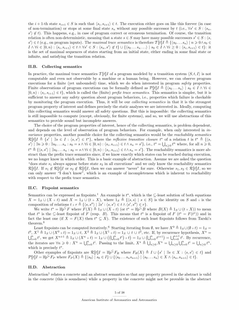
Another example of Galois connection is the Cartesian abstraction, where a set of pairs is abstracted toa pair of sets by projection:

y

x

y

xCartesian abstraction αc Cartesian concretization γc

Given a set X of pairs 〈x, y〉 ∈ X, its abstraction is αc(X) , 〈{x | ∃y : 〈x, y〉 ∈ X}, {y | ∃x : 〈x, y〉 ∈ X}〉.The concretization is γc(〈X,Y 〉) , {〈x, y〉 | x ∈ X ∧ y ∈ Y }. The abstract order ⊆c is componentwiseinclusion. Observe that αc is surjective (onto) and γc is injective (one to one). This is characteristic ofGalois surjections which are Galois connections 〈α, γ〉 such that α is surjective or equivalently γ is injectiveor equivalently α ◦ γ = 1 (where 1 is the identity function: 1(x) = x).

Not all abstractions are Galois connections, in which case one can always use a concretization function.8

A counter-example is provided by a disk, which has no best over-approximation by a convex polyhedron,9

as shown by Euclid.10

a We have α(T ) ⊆] α(T ) so that, by the if part of the definition (with R = α(T )), we get T ⊆ γ(α(T )).b If T ⊆ γ(R) then, by the only if part of the definition, it follows that α(T ) ⊆] R.

6 of 38


II.G. The lattice of abstractions

We have seen that the reachability semantics is more abstract than the prefix trace semantics which ismore abstract than the maximal traces semantics. Some abstractions (such as sign and parity of naturalnumbers) are not comparable. So, abstract properties form a lattice with respect to the relation “is moreabstract than”.1,7 Exploring the world of (collecting) semantics and their lattice of abstractions is one of themain research subjects in abstract interpretation. In particular “finding the appropriate level of abstractionrequired to answer a question” is a recurrent fundamental and practical question.

II.H. Sound (and complete) abstract semantics

Given a concrete semantics S and an abstraction specified by a concretization function γ (respectively anabstraction function α), we are interested in an abstract semantics S] which is sound in that S ⊆ γ(S])(respectively α(S) ⊆] S], which is equivalent for Galois connections). This corresponds to the intuition thatno concrete case is ever forgotten in the abstract (so there can be no false negative). It may also happen thatthe abstract semantics is complete, meaning that S ⊇ γ(S]) (respectively α(S) ⊇] S] c). This correspondsto the intuition that no abstract case is ever absent in the concrete (so there can be no false positive). Theideal case is that of a sound and complete semantics such that S = γ(S]) (respectively α(S) = S]).

The abstractions used in program proof methods (such as αP for Burstall’s intermittent assertions proofmethod11,12 or αR for Floyd’s invariant assertions proof method13,14) are usually sound and complete (but,by undecidability, these abstractions yield proof methods that are not fully mechanizable). The abstractionsused in static program analysis (such as the Cartesian abstraction in Sect. II.F, the interval abstractionin Sect. II.M, or type systems that do reject programs that can never go wrong15) are usually sound andincomplete (but fully mechanizable).

II.I. Abstract transformers

Because the concrete semantics S = lfp⊆F is usually the least fixpoint of a concrete transformer F , onecan attempt to express the abstract semantics in the same fixpoint form S] = lfp⊆

]

F ] for an abstracttransformer F ] where X ⊆] Y if and only if γ(X) ⊆ γ(Y ). The abstract transformer F ] is said to be soundwhen F ◦ γ ⊆ γ ◦ F ] (respectively α ◦ F ⊆] F ] ◦ α d). In case of a Galois connection, there is a “best”abstract transformer, which is F ] , α ◦ F ◦ γ. In all cases, the main idea is that the abstract transformerF ] always over-approximates the result of the concrete transformer F .

II.J. Sound abstract fixpoint semantics

Given a concrete fixpoint semantics S = lfp⊆F , the task of a static analysis designer is to elaborate anabstraction 〈α, γ〉 and then the abstract transformer F ] , α ◦ F ◦ γ (or F ] such that F ◦ γ ⊆ γ ◦ F ] in theabsence of a Galois connection). Under appropriate hypotheses,7 the abstract semantics is then guaranteedto be sound: S = lfp⊆F ⊆ γ(S]) = γ(lfp⊆

]

F ]). Otherwise stated, the abstract fixpoint over-approximatesthe concrete fixpoint, hence preserves the soundness: if S] ⊆] P ] then S ⊆ γ(P ]) (any abstract property P ]

which holds in the abstract also holds for the concrete semantics). This yields the basis to formally verifythe soundness of static analyzers using theorem provers or proof checkers.16

II.K. Sound and complete abstract fixpoints semantics

Under the hypotheses of Tarski’s fixpoint theorem6 and the additional commutation hypothesis7 α ◦ F =F ] ◦ α for Galois connections, we have α(S) = α(lfp⊆F ) = S] = lfp⊆

]

F ]. Otherwise stated, the fact thatthe concrete semantics is a least fixpoint is preserved in the abstract.

For example, RJtKI = lfp⊆FR and αR ◦ FP = FR ◦ αR imply that RJtKI , αR(PJtKI) = αR(lfp⊆FP ) =lfp⊆FR. The intuition is that, to reason on reachable states, it is useless to consider execution traces.Complete abstractions exactly answer the class of questions defined by the abstraction of the collectingsemantics. However, for most interesting questions on programs, the answer is not algorithmic or very severerestrictions have to be considered, such as finiteness.

cWhich in general is not equivalent, even for Galois connections.dWhich is equivalent when 〈α, γ〉 is a Galois connection and F and F ] are increasing.

7 of 38


II.L. Example of finite abstraction: model-checking

Model-checking17 abstracts systems to finite state systems so that partial traces or reachable states can becomputed by finite iterative fixpoint concretization. In fact, Cousot18 showed that any abstraction α to afinite domain D is amenable to model-checking by bit-wise encoding of {γ(P ) | P ∈ D} (where D is thefinite set of abstract properties, e.g., D = ℘(S) for reachability over a finite set S of states).

II.M. Example of infinite abstraction: interval abstraction

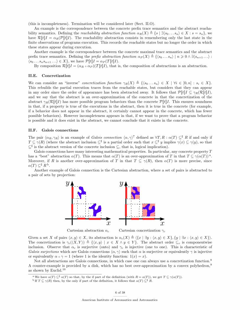
Assume that a program has numerical (integer, float, etc.) variables x ∈ V, so that program states s ∈ S mapeach variable x ∈ V to its numerical value s(x) in state s. An interesting problem on programs is to determinethe interval of variation of each variable x ∈ V during any possible execution. This consists in abstractingthe reachability semantics first by the Cartesian abstraction and then by the interval abstraction:

y

x

y

xInterval abstraction αc Interval concretization γc

This is αι(RJtKI) where αι(X)(x) = [mins∈X s(x), maxs∈X s(x)] which can be ∅ when X is empty andmay have infinite bounds −∞ or +∞ in the absence of a minimum or a maximum. This abstraction isinfinite in that, e.g., [0, 0] ⊆ [0, 1] ⊆ [0, 2] ⊆ · · · ⊆ [0,+∞]. Assuming that numbers are bounded (e.g.,−∞ = minint and +∞ = maxint for integers) yields a finite set of states but this is of no help due tocombinatorial explosion when considering all subsets of states in ℘(S).

One may wonder why infinite abstractions are of any practical interest since computers can only do finitecomputations anyway. The answer comes form a very simple example: P ≡ x=0; while (x<=n) { x=x+1 },where the symbol n > 0 stands for a numerical constant (so that we have an infinite family of programs forall integer constants n = 0, 1, 2, . . .).19 For any given constant value of n, an abstract interpretation-basedanalyzer using the interval abstraction20 will determine that, on loop body entry, x ∈ [0, n] always hold. Ifwe were restricted to a finite domain, we would have only finitely many such intervals, and so, we would findthe exact answer for only finitely many programs while missing the answer for infinitely many programs inthe family. An alternative would be to use an infinite sequence of finite abstractions of increasing precision(e.g., by restricting abstract states to first {1}, then {1, 2}, then {1, 2, 3}, etc.), and run finite analyses untila precise answer is found, but this would be costly and, moreover, the analysis might not terminate or wouldhave to enforce the termination with exactly the same techniques as those used for infinite abstractions(Sect. II.O), without the benefit of avoiding the combinatorial state explosion.

II.N. Abstract domains and functions

Encoding program properties uniformly (e.g., as terms in theorem provers or BDDs21 in model-checking)greatly simplifies the programming and reusability of verifiers. However, it severely restricts the ability forprogrammers of these verifiers to choose very efficient computer representations of abstract properties anddedicated high-performance algorithms to manipulate such abstract properties in transformers. For example,an interval is better represented by the pair of its bounds rather than the set of its points, whatever computerencoding of sets is used.

So, abstract interpretation-based static analyzers and verifiers do not use a uniform encoding of abstractproperties. Instead, they use many different abstract domains which are algebras (for mathematicians) ormodules (for computer scientists) with data structures to encode abstract properties (e.g., either ∅ or apair [`, h] of numbers or infinity for intervals, with ` ≤ h). Abstract functions are elementary functions onabstract properties which are used to express the abstraction of the fixpoint transformers FP , FR, etc.

8 of 38


For example, the interval transformer Fι will use interval inclusion (∅ ⊆ ∅ ⊆ [a, b], [a, b] ⊆ [c, d] if andonly if c 6 a and b 6 d), addition (∅+ ∅ = ∅+ [a, b] = [a, b] + ∅ = ∅ and [a, b] + [c, d] = [a+ c, b+ d]), union(∅ ∪ ∅ = ∅, ∅ ∪ [a, b] = [a, b] ∪ ∅ = [a, b] and [a, b] ∪ [c, d] = [min(a, c),max(b, d)]), etc., which will be basicoperations available in the abstract domain. Public implementations of abstract domains are available suchas Apron22,23 for numerical domains.

II.O. Convergence acceleration by extrapolation

II.O.1. Widening

Let us consider the program x=1; while (true) { x=x+2 }. The interval of variation of variable x is theleast interval solution to the equation X = Fι(X) where Fι(X) , [1, 1] ∪ (X + [2, 2]). Solving iterativelyfrom X0 = ∅, we have X1 = [1, 1] ∪ (X0 + [2, 2]) = [1, 1], X2 = [1, 1] ∪ (X1 + [2, 2]) = [1, 1] ∪ [3, 3] = [1, 3],X3 = [1, 1]∪(X2 +[2, 2]) = [1, 1]∪ [3, 5] = [1, 5], which, after infinitely many iterates and passing to the limit,yields [1,+∞). Obviously, no computer can compute infinitely many iterates, nor perform the reasoning byrecurrence and automatically pass to the limit as humans would do.

An idea is to accelerate the convergence by an extrapolation operator called a widening ,1,5, 20 solvingX = X

`Fι(X) instead of X = Fι(X). The widening

`uses two consecutive iterates Xn and Fι(Xn) in

order to extrapolate the next one Xn+1. This extrapolation should be an over-approximation (Xn ⊆ Xn+1

and Fι(Xn) ⊆ Xn+1) for soundness and enforce convergence for termination. In finite abstract domains,widenings are useless and can be replaced with the union ∪.

An example widening for intervals is x` ∅ = ∅, ∅ `

x = x, [a, b]`

[c, d] , [`, h], where ` = −∞ whenc < a and ` = a when a 6 c. Similarly, h = +∞ when b < d and h = b when d 6 b. The widened interval isalways larger (soundness) and avoids infinitely increasing iterations (e.g., [0,0], [0,1], [0,2], etc.) by pushingto infinity limits that are unstable (termination).

For the equation X = X`Fι(X) where Fι(X) , [1, 1] ∪ (X + [2, 2]), the iteration is now X0 = ∅,

X1 = X0 `([1, 1]∪(X0 +[2, 2])) = ∅`

[1, 1] = [1, 1], X2 = X1 `([1, 1]∪(X1 +[2, 2])) = [1, 1]

`[1, 3] = [1,+∞),

X3 = X2 `([1, 1]∪ (X2 + [2, 2])) = [1,+∞)

`[1,+∞) = [1,+∞) = X2, which converges to a fixpoint in only

three steps.

II.O.2. Narrowing

For the program, x=1; while (x<100) { x=x+2 }, we would have X = X`Fι(X) where Fι(X) , [1, 1] ∪

((X+[2, 2])∩(−∞, 99]) with iterates X0 = ∅, X1 = X0`([1, 1]∪((X0+[2, 2])∩(−∞, 99])) = ∅`

[1, 1] = [1, 1],X2 = X1 `

([1, 1] ∪ ((X1 + [2, 2]) ∩ (−∞, 99])) = [1, 1]`

[1, 3] = [1,+∞).After that upwards iteration (where intervals are wider and wider), we can go on with a downwards

iteration (where intervals are narrower and narrower). To avoid infinite decreasing chains (such as [0,+∞),[1,+∞), [2,+∞), . . . , which limit is ∅), we use an extrapolation operator called a narrowing1,5 a

for theequation X = X

aFι(X). The narrowing should ensure both soundness and termination. In finite abstract

domains, narrowings are useless and can be replaced with the intersection ∩.An example of narrowing for intervals is ∅ a

x = ∅, x a ∅ = ∅, [a, b]a

[c, d] = [`, h] where ` = c whena = −∞ and ` = a when a 6= −∞ and similarly h = d when b = +∞ and otherwise h = b. So, infinitebounds are refined but not finite ones, so that the limit of [0,+∞), [1,+∞), [2,+∞), . . . , ∅ will be roughlyover-approximated as [0,+∞). This ensures the termination of the iteration process. The narrowed interval[a, b]

a[c, d] is wider than [c, d], which ensures soundness.

For the program x=1; while (x<100) { x=x+2 }, the downwards iteration is now Y = YaFι(Y )

starting from the fixpoint obtained after widening: Y 0 = [1,+∞), Y 1 = Y 0 a([1, 1] ∪ ((Y 0 + [2, 2]) ∩

(−∞, 99])) = [1,+∞)a

([1, 1]∪ ([3,+∞)∩ (−∞, 99])) = [1,+∞)a

[1, 99] = [1, 99]. The next iterate is Y 2 =Y 1 a

([1, 1]∪((Y 1 +[2, 2])∩(−∞, 99])) = [1, 99]a

([1, 1]∪([3, 101]∩(−∞, 99])) = [1, 99]a

[1, 99] = [1, 99] = Y 1

so that a fixpoint is reached (although it may not be the least one, in general).Of course, for finite abstractions (where strictly increasing chains are finite) no widening nor narrowing

is needed since the brute-force iteration in the finite abstract domain always terminates. However, to avoida time and space explosion, convergence acceleration with widening and narrowing may be helpful (at theprice of incompleteness in the abstract, which is present anyway in the concrete except for finite transitionsystems).

9 of 38


II.P. Combination of abstract domains

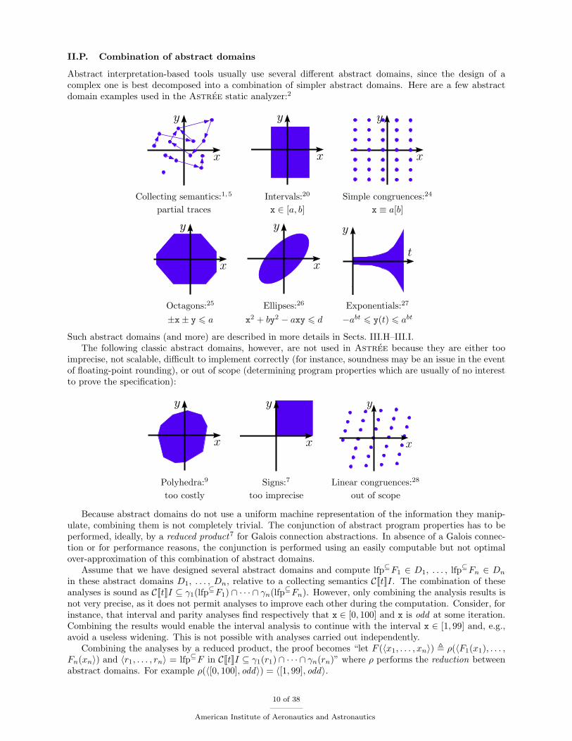
Abstract interpretation-based tools usually use several different abstract domains, since the design of acomplex one is best decomposed into a combination of simpler abstract domains. Here are a few abstractdomain examples used in the Astree static analyzer:2

x

y

x

y

x

y

Collecting semantics:1,5 Intervals:20 Simple congruences:24

partial traces x ∈ [a, b] x ≡ a[b]

x

y

x

y

t

y

Octagons:25 Ellipses:26 Exponentials:27

±x± y 6 a x2 + by2 − axy 6 d −abt 6 y(t) 6 abt

Such abstract domains (and more) are described in more details in Sects. III.H–III.I.The following classic abstract domains, however, are not used in Astree because they are either too

imprecise, not scalable, difficult to implement correctly (for instance, soundness may be an issue in the eventof floating-point rounding), or out of scope (determining program properties which are usually of no interestto prove the specification):

x

y

x

y

x

y

Polyhedra:9 Signs:7 Linear congruences:28

too costly too imprecise out of scope

Because abstract domains do not use a uniform machine representation of the information they manip-ulate, combining them is not completely trivial. The conjunction of abstract program properties has to beperformed, ideally, by a reduced product7 for Galois connection abstractions. In absence of a Galois connec-tion or for performance reasons, the conjunction is performed using an easily computable but not optimalover-approximation of this combination of abstract domains.

Assume that we have designed several abstract domains and compute lfp⊆F1 ∈ D1, . . . , lfp⊆Fn ∈ Dn

in these abstract domains D1, . . . , Dn, relative to a collecting semantics CJtKI. The combination of theseanalyses is sound as CJtKI ⊆ γ1(lfp⊆F1) ∩ · · · ∩ γn(lfp⊆Fn). However, only combining the analysis results isnot very precise, as it does not permit analyses to improve each other during the computation. Consider, forinstance, that interval and parity analyses find respectively that x ∈ [0, 100] and x is odd at some iteration.Combining the results would enable the interval analysis to continue with the interval x ∈ [1, 99] and, e.g.,avoid a useless widening. This is not possible with analyses carried out independently.

Combining the analyses by a reduced product, the proof becomes “let F (〈x1, . . . , xn〉) , ρ(〈F1(x1), . . . ,Fn(xn〉) and 〈r1, . . . , rn〉 = lfp⊆F in CJtKI ⊆ γ1(r1) ∩ · · · ∩ γn(rn)” where ρ performs the reduction betweenabstract domains. For example ρ(〈[0, 100], odd〉) = 〈[1, 99], odd〉.

10 of 38


To define ρ, first consider the case of two abstract domains. The conjunction of p1 ∈ D1 and p2 ∈ D2 isγ1(p1)∩γ2(p2) in the concrete, which is over-approximated as α1(γ1(p1)∩γ2(p2)) in D1 and α2(γ1(p1)∩γ2(p2))in D2. So, the reduced product of D1 and D2 is {ρ12(〈p1, p2〉) | p1 ∈ D1 ∧ p2 ∈ D2}, where the reduction isρ12(〈p1, p2〉) , 〈α1(γ1(p1) ∩ γ2(p2)), α2(γ1(p1) ∩ γ2(p2))〉.

If more than two abstract domains are considered, a global reduction ρ can be defined by iterating thetwo-by-two reductions ρij , i 6= j until a fixpoint is reached. For the sake of efficiency, an over-approximationof the reduced product can be used, where only some of the reductions ρij are applied, in a fixed order.29

These reduction ideas also apply in absence of Galois connection; detailed examples are given in Sect. III.J.

II.Q. Partitioning abstractions

Another useful tool to design complex abstractions from simpler ones is partitioning .30 In its simplest form,it consists in considering a collecting semantics on a powerset concrete domain C = ℘(S), and a finitepartition S1, . . . , Sn of the set S. Each part ℘(Si) is abstracted by an abstract domain Di (possibly the samefor all partitions). An abstract element is thus a tuple 〈d1, . . . , dn〉 ∈ D1 × · · · × Dn, with concretizationγ(〈d1, . . . , dn〉) , (γ1(d1) ∩ S1) ∪ · · · ∪ (γn(dn) ∩ Sn) and abstraction α(X) , 〈α1(X ∩ S1), . . . , αn(X ∩ Sn)〉.For instance, one may consider refining the interval domain by maintaining a distinct interval for positivevalues and for negative values of x: γ(〈[`+, h+], [`−, h−]〉) , ([`+, h+]∩ [0,+∞))∪ ([`−, h−]∩ (−∞, 0)). Thisdomain can represent some disjoint sets (such as the set of non-zero integers (−∞,−1]∪ [1,+∞)), while thenon-partitioned interval domain cannot.

Instead of a partition S1, . . . , Sn of S, one can choose a covering of S. In this case, several syntacticallydistinct abstract elements may represent the same concrete element, but this does not pose any difficulty.It is also possible to choose an infinite family of sets (Si)i∈N covering S such that each element of ℘(S) canbe covered by finitely many parts in (Si)i∈N . A common technique31 is to choose the family (Si)i∈N as anabstract domain, so that, given two abstract domainsDs andDd, the partitioning ofDd overDs is an abstractdomain containing finite sets of pairs in Ds ×Dd, where γ(〈〈s1, d1〉, . . . , 〈sn, dn〉〉 ,

⋃ni=1 γs(si) ∩ γd(di).

Later sections present examples of partitioning abstractions for program control states (Sect. III.C),program traces (Sect. III.E), and program data states (Sect. III.H.4).

II.R. Static analysis

Static analysis consists in answering an implicit question of the form “what can you tell me about thecollecting semantics of this program?”, e.g., “what are the reachable states?”. Because the problem isundecidable, we provide an over-approximation by automatically computing an abstraction of the collectingsemantics. For example, interval analysis20 over-approximates lfp⊆Fι using widening and narrowing. Thebenefit of static analysis is to provide complex information about program behaviors without requiringend-users to provide specifications.

An abstract interpretation-based static analyzer is built by combining abstract domains, e.g., in orderto automatically compute abstract program properties in D = D1 × · · · ×Dn. This consists in reading theprogram text from which an abstract transformer FD is computed using compilation techniques. Then, anover-approximation of lfp⊆FD is computed by iteration with extrapolation by widening and narrowing. Thisabstract property can be interactively reported to the end-user through an interface or used to check anabstract specification.

II.S. Abstract specifications

A specification is a property of the program semantics. Because the specification must be specified relativeto a program semantics, we understand it with respect to a collecting semantics. For example, a reachabilityspecification often takes the form of a set B ∈ ℘(S) of bad states (so that the good states are the complementS \B). The specification is usually given at some level of abstraction. For example, the interval of variationof the values of a variable x at execution is always between two bounds [`x, hx].

II.T. Verification

The verification consists in proving that the collecting semantics implies the specification. For example thereachability specification with bad states B ∈ ℘(S) is RJtKI ⊆ (S \ B), that is, “no execution can reach a

11 of 38


bad state”. Because the specification is given at some level of abstraction, the verification needs not be donein the concrete.

For the interval example, we would have to check ∀x ∈ V : αι(RJtKI)(x) ⊆ [`x, hx]. To do that, wemight think of checking with the abstract interval semantics IJtKI(x) ⊆ [`x, hx], where the abstract intervalsemantics IJtK is an over-approximation in the intervals of the reachability semantics RJtK. This means thatIJtKI(x) ⊇ αι(RJtKI)(x). Observe that ∀x ∈ V : IJtKI(x) ⊆ [`x, hx] implies αι(RJtKI)(x) ⊆ [`x, hx], proving∀x ∈ V,∀s ∈ RJtKI : s(x) ∈ [`x, hx] as required.

II.U. Verification in the abstract

Of course, as in mathematics, to prove a result, a stronger one is often needed. So, proving specifications atsome level of abstraction often requires much more precise abstractions of the collecting semantics.

An example is the rule of signs pos × pos = pos, neg × neg = pos, pos × neg = neg, etc., whereγ(pos) , {z ∈ Z | z > 0} and γ(neg) , {z ∈ Z | z 6 0}). The sign abstraction is complete for multiplication(knowing the sign of the arguments is enough to determine the sign of the result) but incomplete for addition(pos + neg is unknown). However, if an interval is known for the arguments of an addition, the interval ofthe result, hence its sign, can be determined for sure. So, intervals is the most abstract abstraction which iscomplete for determining the sign of additions.

In general, a most abstract complete abstraction to prove a given abstract specification does exist32 but isunfortunately uncomputable, even for a given program. In practice, one uses a reduced product of differentabstractions which are enriched by new ones to solve incompleteness problems, a process which, by unde-cidability, cannot be fully automatizable — e.g., because designing efficient data structures and algorithmsfor abstract domains is not automatizable (see for example Sect. III.I.1), which is a severe limitation ofautomatic refinement of abstractions.33

III. Verification of Synchronous Control/Command Programs

We now briefly discuss Astree, a static analyzer for automatically verifying the absence of runtimeerrors in synchronous control/command embedded C programs2,29,34–37 successfully used in aeronautics3

and aerospace4 and now industrialized by AbsInt.38,39

III.A. Subset of C analyzed

Astree can analyze a fairly large subset of C 99. The most important unsupported features are: dynamicmemory allocation (malloc), non-local jumps (longjmp), and recursive procedures. Such features are mostoften unused (or even forbidden) in embedded programming to keep a strict control on resource usage andcontrol-flow. Parallel programs are also currently unsupported (although parallel constructs are not strictlyspeaking in the language, but rather supported by special libraries), but some progress is made to supportthem (Sect. VI).

Although Astree can analyze many programs, it cannot analyze most of them precisely and efficiently.Astree is specialized for control/command synchronous programs, as per the choice of included abstractions.Some generic existing abstractions were chosen for their relevance to the application domain (Sect. III.H),while others were developed specially for it (Sect. III.I).

Astree can only analyze stand-alone programs, without undefined symbols. That is, if a program callsexternal libraries, the source-code of the libraries must be provided. Alternatively, stubs may be providedfor library functions, to provide sufficient semantic information (range of return values, side-effects, etc.) forthe analysis to be carried out soundly. The same holds for input variables set by the environment, the rangeof which may have to be specified.

III.B. Operational semantics of C

Astree is based on the C ISO/IEC 9899:1999/Cor 3:2007 standard,40 which describes precisely (if infor-mally) a small-step operational semantics. However, the standard semantics is high-level, leaving many be-haviors not fully specified so that implementations are free to choose their semantics (ranging from producinga consistent, documented outcome, to considering the operation as undefined with catastrophic consequences

12 of 38


when executed). Sticking to the norm would not be of much practical use for our purpose, that is, to ana-lyze embedded programs that are generally not strictly conforming but rely instead on specific features ofa platform, processor, and compiler. Likewise, Astree makes semantics assumptions, e.g., on the binaryrepresentation of data-types (bit-size, endianess), the layout of aggregate data-types in memory (structures,arrays, unions), the effect of integer overflows, etc. These assumptions are configurable by the end-user tomatch the actual target platform of the analyzed program (within reasonable limits corresponding to modernmainstream C implementations), being understood that the result of an analysis is only sound with respectto the chosen assumptions.

Astree computes an abstraction of the semantics of the program and emits an alarm whenever it leadsto a runtime error. Runtime errors that are looked for include: overflows in unsigned or signed integer or floatarithmetics, integer or float divisions or modulos by zero, integer shifts by an invalid amount, values outsidethe definition of an enumeration, out-of-bound array accesses, dereferences of a NULL or dangling pointer,of a mis-aligned pointer, or outside the space allocated for a variable. In case of an erroneous execution,Astree continues with the worst-case assumption, such as considering that, after an arithmetic overflow,the result may be any value allowed by the expression type (although, in this case, the user can instructAstree to assume that a modular semantics should be used instead). This allows Astree to find all furthererrors following any error, whatever the actual semantics of errors chosen by the implementation. Sometimes,however, the worst possible scenario after a runtime error is completely meaningless (e.g., accessing a danglingpointer which destroys the program code), in which case Astree continues the analysis for the non-erroneouscases only. An execution of the program performing the erroneous operation may not actually fail at thepoint reported by Astree and, instead, exhibit an erratic behavior and fail at some later program point notreported by Astree. In all cases, the program has no runtime error if Astree does not issue any alarm, orif all executions leading to alarms reported by Astree can be proved, by external means, to be impossible.

III.C. Flow- and context-sensitive abstractions

Static analyses are often categorized as being either flow-sensitive or flow-insensitive, and either context-sensitive or context-insensitive. The former indicates whether the analysis can distinguish properties holdingat some control point and not other ones, and the later whether the analyzer distinguishes properties atdistinct call contexts of the same procedure.

Astree is both flow- and context-sensitive, where a call context means here the full sequence of nestedcallers. Indeed, in the collecting semantics, the set of program states S is decomposed into a control and adata components: S , C×D. The control component C contains the syntactic program location of the nextinstruction to be executed, as well as the stack of the program locations in the caller functions indicatingwhere to jump back after a return instruction. The data component D contains a snapshot of the memory(value of global variables and local variables for each activation record). Full flow- and context-sensitivity isachieved by partitioning (Sect. II.Q), i.e., keeping an abstraction of the data state D (Sect. III.F) for eachreachable control state in C. This simple partitioning simplifies the design of the analysis while permitting ahigh precision. However, it limits the analyzer to programs with a finite set of control states C, i.e., programswithout unbounded recursion. This is not a problem for embedded software, where the control space is finite,and indeed rather small. More abstract control partitioning abstractions must be considered in cases whereC is infinite or very large (e.g., for parallel programs, as discussed in Sect. VI).

III.D. Hierarchy of parameterized abstractions

Astree is constructed in a modular way. In particular, it employs abstractions parameterized by abstrac-tions, which allows constructing a complex abstraction from several simpler ones (often defined on a less richconcrete universe). Indeed, although Astree ultimately abstracts a collecting semantics of partial traces,the trace abstraction is actually a functor able to lift an abstraction of memory states (viewed as maps fromvariables in V to values in V) to an abstraction of state traces (viewed as sequences in (C × (V → V))∗). Ithandles all the trace-specific aspects of the semantics, and delegates the abstraction of states to the memorydomain. The memory abstraction is in turn parameterized by a pointer abstraction, itself parameterized bya numerical abstraction, where each abstraction handles simpler and simpler data-types. This gives:

13 of 38


trace abstraction of ℘((C × (V→ V))∗) (Sect. III.E)↓

memory abstraction of ℘(V→ V) (Sect. III.F)↓

pointer abstraction of ℘(Vc → Vb) (Sect. III.G)↓

product of numerical abstractions of ℘(Vn → R) (Sects. III.H–III.I)

An improvement to any domain will also benefit other ones, and it is easy to replace one module parameterwith another. The numerical abstraction is itself a large collection of abstract domain modules with thesame interface (i.e., abstracting the same concrete semantics) linked through a reduced product functor(Sect. III.J), which makes it easy to add or remove such domains.

III.E. Trace abstraction

Floyd’s method13 is complete in the sense that all invariance properties can be proved using only stateinvariants, that is, sets of states. However, this does not mean it is always the best solution, in the sensethat such invariants are not always the easiest to represent concisely or compute efficiently. It is sometimesmuch easier to use intermittent invariants as in Burstall’s proof method11 (i.e., an abstraction of the partialtrace semantics12).

In particular, in many numerical abstract domains, all abstract values represent convex sets of states (forinstance, this is the case of intervals, octagons, polyhedra): this means that the abstract join operation willinduce a serious loss of precision in certain cases. For instance, if variable x may take any value except 0,and if the analysis should establish this fact in order to prove the property of interest (e.g., that a divisionby x will not crash), then we need to prevent states where x > 0 from being confused with states wherex < 0. As a consequence, the set of reachable states of the program should be partitioned carefully so as toavoid certain subsets be joined together. In other words, context sensitivity (Section III.C) is not enough toguarantee a high level of precision, and some other mechanisms to distinguish sets of reachable states shouldbe implemented.

The main difficulty which needs to be solved in order to achieve this is to compute automatically goodpartitions. In many cases, such information can be derived from the control-flow of the program to analyze(e.g., which branch of some if-statement was executed or how many times the body of some loop wasexecuted). In other cases, a good choice of partitions can be provided by a condition at some point in theexecution of the program, such as the value of a variable at the call site of a function.

To formalize this intuition, we can note that it amounts to partitioning the set of reachable states ateach control state, depending on properties of the whole executions before that point is reached. This isthe reason why Astree abstracts partial traces rather than just reachable states. An element of the tracepartitioning abstract domain41,42 should map each element of a a finite partition of the traces of the programto an abstract invariant. Thus, it is a partitioning abstraction (Sect. II.Q), at the level of traces.

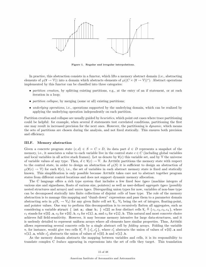
Let us consider a couple of examples illustrating the impact of trace partitioning. Embedded softwareoften need to compute interpolation functions (in one, two, or more dimensions). In such functions, a fixedinput grid is supplied together with output values for each point in the grid. Typical interpolation algorithmsfirst localize in which cell in the grid the input is, and then apply linear or non-linear local interpolationformulas. In the case of regular grids as in the left of Fig. 1, the localization can be done using simplearithmetic, whereas in the more general case of non-regular grids, as in the right, localizing the input may bedone using a search loop. In all cases, the interpolation can be precisely analyzed only if a close relationshipbetween the input values and the grid cells can be established, so that the right interpolation formula canbe applied to the right (abstract) set of inputs. Trace partitioning allows expressing such relations, withinvariants which consist in conjunctions of properties of the form “if the input is in cell i, then the currentstate satisfies condition pi”. This is possible since the cell the input is contained in is an abstraction ofthe history of the execution: for instance, when the cell is determined using a loop, it is determined bythe number of iterations spent in that loop. Such invariants allow for a fine analysis of such codes, sinceit amounts to analyzing the interpolation function “cell by cell”. Last, we can note that this partitioningshould only be local, for efficiency reasons.

14 of 38


x

y

b

bb

b

b

b

b

b

b

b

b

b

bb

b

bb

x

y

b

b

b

b

b

b

b

Figure 1. Regular and irregular interpolations.

In practice, this abstraction consists in a functor, which lifts a memory abstract domain (i.e., abstractingelements of ℘(V → V)) into a domain which abstracts elements of ℘((C × (V → V))∗). Abstract operationsimplemented by this functor can be classified into three categories:

• partition creation, by splitting existing partitions, e.g., at the entry of an if statement, or at eachiteration in a loop;

• partition collapse, by merging (some or all) existing partitions;

• underlying operations, i.e., operations supported by the underlying domain, which can be realized byapplying the underlying operation independently on each partition.

Partition creation and collapse are usually guided by heuristics, which point out cases where trace partitioningcould be helpful: for example, when several if statements test correlated conditions, partitioning the firstone may result in increased precision for the next ones. However, the partitioning is dynamic, which meansthe sets of partitions are chosen during the analysis, and not fixed statically. This ensures both precisionand efficiency.

III.F. Memory abstraction

Given a concrete program state (c, d) ∈ S = C × D, its data part d ∈ D represents a snapshot of thememory, i.e., it associates a value to each variable live in the control state c ∈ C (including global variablesand local variables in all active stack frames). Let us denote by V(c) this variable set, and by V the universeof variable values of any type. Then, d ∈ V(c) → V. As Astree partitions the memory state with respectto the control state, in order to design an abstraction of ℘(S) it is sufficient to design an abstraction of℘(V(c) → V) for each V(c), i.e., the set of variables in each abstract memory state is fixed and staticallyknown. This simplification is only possible because Astree takes care not to abstract together programstates from different control locations and does not support dynamic memory allocation.

The C language offers a rich type system that includes a few fixed base types (machine integers ofvarious size and signedness, floats of various size, pointers) as well as user-defined aggregate types (possiblynested structures and arrays) and union types. Disregarding union types for now, variables of non-base typecan be decomposed statically into finite collections of disjoint cells of base type. The role of the memoryabstraction is to manage this mapping and “dumb down” expressions and pass them to a parameter domainabstracting sets in ℘(Vc → Vb) for any given finite cell set Vc, Vb being the set of integers, floating-point,and pointer values. One way to perform this decomposition is to recursively flatten all aggregates, such asconsidering a variable struct { int a; char b; } v[2] as four distinct cells Vc , { c1, c2, c3, c4 }, wherec1 stands for v[0].a, c2 for v[0].b, c3 for v[1].a, and c4 for v[1].b. This natural and most concrete choiceachieves full field-sensitivity. However, it may become memory intensive for large data-structures, and itis uselessly detailed to represent uniform arrays where all elements have similar properties. Thus, Astreeallows representing several concrete cells by a single abstract cell by folding arrays. Folding the variablev, for instance, would give two cells V′c , { c′1, c′2 }, where c′1 abstracts the union of values of v[0].a andv[1].a, while c′2 abstracts the union of values of v[0].b and v[1].b.

As the memory domain abstracts the mapping between variables and cells, it is its responsibility totranslate complex C lvalues appearing in expressions into the set of cells they target. This translation

15 of 38


is dynamic and may depend on the computed (abstract) set of possible variable values at the point ofthe expression, hence the necessary interaction between the memory abstraction and its parameter abstractdomain. Consider, for instance, the assignment v[i].a = v[0].b + 1 to be translated into the cell universeVc , { c1, c2, c3, c4 } (the case of pointer access is considered in Sect. III.G). Depending on the possibleabstract value of i (exemplified here in the interval domain), it can be translated into either c1 = c2 + 1 (ifi is [0, 0]), c3 = c2 + 1 (if i is [1, 1]), or if (?) c1 = c2 + 1 else c3 = c2 + 1 (if i is [0, 1]). This laststatement involves a non-deterministic choice (so-called “weak update”), hence a loss of precision. Valuesof i outside the range [0, 1] lead to runtime errors that stop the program. If the folded memory abstractionV′c , { c′1, c′2 } is considered instead, then the statement is interpreted as if (?) c′1 = c′2 + 1 whatever thevalue of i, which always involves a non-deterministic choice (hence, is less precise).

We now discuss the case of union types. Union types in C allow reusing the same memory block torepresent values of different types. Although not supported by the C 99 standard40 (except in very restrictedcases), it is possible to write a value to a union field, and then read back from another field of the sameunion; the effect is to reinterpret (part of) the byte-representation of a value of the first field type as thebyte-representation of a value of the second type (so-called type punning). This is used to some extent inembedded software, and so, it is supported in Astree. As for aggregate types, union types are decomposedinto cells of base type. Unlike aggregate types, such cells are not actually disjoint, as modifying one unionfield also has an effect on other union fields. However, the memory domain hides this complexity from itsparameter domain, which can consider them as fully distinct entities. The memory domain will issue extracell-based statements to take aliasing into account.43 Consider, for instance, the variable union { unsignedchar c; unsigned int i; } v with two cells: cc for v.c, and ci for v.i. Any write to v.i will update ciand also generate the assignment cc = ci & 255 (assuming the user configured the analyzer for a little endianarchitecture). The memory domain of Astree thus embeds a partial knowledge of the bit-representation ofinteger and floating-point types.

III.G. Pointer abstraction

Pointers in C can be used to implement references as found in many languages, but also generalized arrayaccess (through pointer arithmetics) and type punning (through pointer conversion). To handle all theseaspects in our concrete operational semantics, a pointer value is considered as either a pair 〈v, o〉 composedof a variable v and an integer offset o, or a special NULL or dangling value. The offset o counts a number ofbytes from the beginning of the variable v, and ranges in [0, sizeof(v)).

A set of pointer values is then abstracted in Astree as a pair of flags indicating whether the pointercan be NULL or dangling, a set of variables (represented in extension), and a set of offset values. The pointerabstract domain maintains this information for each cell of pointer type, except for the offset abstractionwhich is delegated to a numerical domain through the creation of a cell of integer type. Moreover, pointerarithmetics is converted into integer arithmetics on offsets. Consider, for instance, the pointer assignmentq = p + i + 1, where p and q have type int*, which is translated into cq = cp + ci + 1 by the memorydomain, where cp, cq, and ci are the cells associated with respectively p, q, and i. The pointer domainthen replaces the pointed-to variable set component of q with that of p and passes down to the numericalabstraction the statement co(q) = co(p) + (ci + 1) * sizeof(int), where co(q) and co(p) are the integer-valued cells corresponding to the offset components of p and q.

Additionally, the pointer abstraction is used by the memory domain to resolve dereferences in expres-sions. For instance, given the lvalue *(p + i), the memory domain relies on the pointer domain to providethe target of cp + ci, which is returned as a set of variable/offset pairs (involving offset computation inthe parameter numerical domain) and possibly NULL or dangling. To handle type punning, the memoryabstraction is able to generate a cell for any combination of a variable, an offset (smaller than the variablebyte-size), and a base type, while NULL and dangling accesses are considered runtime errors. Cells thatoverlap in memory are handled as in the case of union types.

III.H. General-purpose numerical abstractions

Through a sequence of trace, memory, and pointer abstractions, we are left to the problem of abstractingconcrete sets of the form ℘(Vn → R), for any finite set Vn of numerical cells. This is achieved by usinga combination of several numerical abstract domains. Note that the concrete semantics is expressed usingreals R as they include all integers and (non-special) floating-point values for all C implementations.

16 of 38


III.H.1. Intervals

The interval abstract domain1,20 maintains a lower and an upper bound for every integer and floating-pointcell. This is one of the simplest domain, yet its information is crucial to prove the absence of many kinds ofruntime errors (overflows, out-of-bound array accesses, invalid shifts). Most abstract operations on intervalsrely on well-known interval arithmetics.44 Soundness for abstract floating-point operations (considering allpossible rounding directions) is achieved by rounding lower bounds downwards and upper bound upwardswith the same bit-precision as that of the corresponding concrete operation.

An important operation specific to abstract interpretation is the widening`

used to accelerate loops.Astree refines the basic interval widening (recalled in Sect. II.O) by using thresholds: unstable bounds arefirst enlarged to a finite sequence of coarser and coarser bounds before bailing out to infinity. For manyfloating-point computations that are naturally stable (for instance while (1) { X = X * α + [0, β]; },which is stable at X ∈ [0, β/(1 − α)] when α ∈ [0, 1)), a simple exponential ramp is sufficient (X will bebounded by the next threshold greater than β/(1 − α)). Some thresholds can also be inferred from thesource code (such as array bounds, to use for integer cells used as array indices). Finally, other abstractdomains can dynamically hint at (finitely many) new guessed thresholds.

One benefit of the interval domain is its very low cost: O(|Vc|) in memory and time per abstract operation.Moreover, the worst-case timeO(|Vc|) can be significantly reduced to a practicalO(log |Vc|) cost by a judiciouschoice of data-structures. It is sufficient to note that binary operations (such as ∪) are often applied toarguments with only a few differing variables. Astree uses a functional map data-structure with sharingto exploit this property. This makes the interval domain scalable to tens of thousands cells.

III.H.2. Abstraction of floating-point computations

Many control/command software rely on computations that are designed with the perfect semantics of realsR in mind, but are actually implemented using hardware float arithmetics, which incurs inaccuracies dueto pervasive rounding. Rounding can easily accumulate to cause unexpected overflows or divisions by zeroin otherwise well-defined computations. An important feature of Astree is its sound support for floatcomputations following the IEEE 754–198545 semantics.

Reasoning on float arithmetics is generally difficult because, due to rounding, most mathematical prop-erties of operations are no longer true, for instance, the associativity and distributivity of + and ×. Mostnumerical abstract domains in Astree rely on symbolic manipulations of expressions (such as linear alge-bra) that would not be sound when replacing real operators with float ones (one exception being intervalarithmetics, which is easy to implement using float arithmetics on bounds). Thus, Astree implements anabstract domain46,47 able to soundly abstract expressions, i.e., a function f : X → Y is abstracted as a(non-deterministic) function g : X → ℘(Y ) such that f(x) ∈ g(x), at least for all x in some given reachablesubset R of X. g can then be soundly used in place of f , for all arguments in R. In practice, a float ex-pression f(~V) appearing in the program source is abstracted as a linear expression with interval coefficientsg(~V) = [α, β]+

∑i[αi, βi]×Vi, and R is some condition on the bounds of variables. g can be fed to abstract do-

mains on reals as + and × in g denote real additions and multiplications. Interval linear expressions can easilybe manipulated symbolically (they form an affine space), while the intervals provide sufficient expressivenessto abstract away complex non-linear effects (such as rounding or multiplication) as non-determinism. For in-stance, the C statement Z = X + 2.f * Y, where X, Y, and Z are single-precision floats, will be linearized as[1.9999995, 2.0000005]Y+[0.99999988, 1.0000001]X+[−1.1754944×10−38, 1.1754944×10e−38]. Alternatively,under the hypothesis X, Y ∈ [−100, 100], it can be linearized as 2Y+X+[−5.9604648×10−5, 5.9604648×105],which is simpler (variable coefficients are scalars) but exhibits a larger constant term (i.e., absolute roundingerror).

An additional complexity in float arithmetics is the presence (e.g., in inputs) of special values +∞, −∞,and NaN (Not a Number), as well as the distinction between +0 and −0. Thus, a float type is almostbut not exactly a finite subset of R. The presence of a special value is abstracted as a boolean flag in theabstraction of each float cell, while 0 actually abstracts both concrete values +0 and −0. Astree checksthat an expression does not compute any special value before performing symbolic manipulations definedonly over R.

Note that, because all operations in the expression abstract domain can be broken down to real intervalarithmetics, it can be soundly implemented using float arithmetics with outwards rounding, which guaranteesits efficiency. Other, more precise abstractions of float computations48 exist, but are not used in Astree as

17 of 38


they are more costly while the extra precision is not useful when checking solely for the absence of runtimeerrors.

III.H.3. Octagons

Given a finite set Vn of numerical cells, we denote by Oct(Vn) the subset of linear expressions Oct(Vn) ,{±X ± Y | X, Y ∈ Vn }. The octagon domain25,47,49 abstracts a concrete set of points X ∈ ℘(Vn → R) asαOct(X) , {maxx∈X e(x) | e ∈ Oct(Vn) }, that is, the tightest set of constraints of the form ±X± Y ≤ c (i.e.,with c minimal) that enclose X. The name octagon comes from the shape of αOct(X) in two dimensions.

The octagon domain is able to express relationships between variables (unlike non-relational domains,such as the interval domain). For instance, it can discover that, after the test if (X>Y) X=Y, the relationX ≤ Y holds. If, later, the range of Y is refined, as per a test if (Y<=10), it can use this information todeduce that X ≤ 10. Although X ≤ 10 is an interval property, the interval domain does not have the necessarysymbolic power to infer it. Another example is the case of loops, such as for (i=0,x=0; i<1000; i++){ if (?) x++; if (?) x=0; }, where the octagon domain finds the symbolic relation x ≤ i for the loophead, although x and i are never explicitly assigned nor tested together. As i = 1000 when the loop exits,we also have x ∈ [0, 1000]. The interval domain can find the former (using widenings and narrowings) butnot the later (no test on x refines the result [0,+∞) after widening), while the octagon domain finds both.

The octagon domain is based on a matrix data-structure50 with memory cost O(|Vn|2), and shortest-path closure algorithms with time cost O(|Vn|3). This is far less costly than general polyhedra9 (which haveexponential cost), yet octagons correspond to a class of linear relations common in programs. As the intervaldomain, the octagon domain can be implemented efficiently in float arithmetics. Moreover, it can abstractinteger (including pointer offset) and float arithmetics (provided these are linearized, as in Sect. III.H.2),and even infer relationships between cells of different type.

III.H.4. Decision trees

The octagons abstract domain expresses linear numerical relations. However, other families of relations haveto be expressed and inferred, in order to ensure the success of the verification of absence of runtime errors.In particular, when some integer variables are used as booleans, relations of the form “if x is (not) equal to0 then y satisfies property P” may be needed, especially if part of the control-flow is stored into booleanvariables.

For instance, let us consider the program b = (x >= 6); ... if (b) y = 10 / (x - 4);. This pro-gram is safe in the sense that no division by 0 will occur, since the division is performed only when b denotesthe boolean value true (i.e., is not equal to 0), that is only when x is greater than 6 (so that x - 4 is not0). However, this property can be proved only if a relation between b and x is established: otherwise, if noinformation is known about x at the beginning of the program, no information will be gained at the entryof the true branch of the if statement, so that a division by 0 alarm should be raised. In such cases, linearconstraints are of no help, since only the boolean denotation of b matters here. Thus, we use a relationalabstraction where some variables are treated as boolean whereas other variables are treated as pure numericvariables. Abstract values consist in decision trees containing numeric invariants at the leaves. Internalnodes of the trees are labeled by boolean variables and the two sub-trees coming out of an internal nodecorrespond to the decision on whether that variable is true or false. The kind of invariants that can be storedat the leaves is a parameter of the domain. By default in Astree, the leaf abstract domain is the product ofbasic inexpensive domains, such as the interval or equality abstract domains. The concretization of such atree comprises all the stores which satisfy the numeric condition which can be read at the leaf of the uniquebranch which it satisfies (i.e., such that it maps each variable into the boolean value assigned to it on thebranch). In the above example, the decision tree we need simply states that “when b is true, x is greaterthan 6”.

This abstraction retains some of the properties of binary decision diagrams:51 the efficiency is greatlyimproved by ordering the boolean variables and using sub-tree sharing techniques.

This abstract domain defines a form of partitioning in the sense of Sect. II.Q: given a boolean tree, we canexpress its concretization as the join of the concretization of the boolean condition at each leaf intersectedwith a set of states depending on the branch. Yet, it operates in a very different manner compared totrace partitioning (Sect. III.E): indeed, the boolean decision trees abstract domain is based on partitionsof the set of states, and not traces. This remark has a great impact on the definition of transfer functions:

18 of 38


partitions are not affected by control-flow branches; however, when an assignment is made, partitions maybe modified. For instance, if a program contains the assignment x = x || y, then some partitions need tobe merged (after the assignment, x is true if and only if either x or y was true before) or intersected (afterthe assignment, x is false if and only if both x and y were false before).

III.H.5. Packing

Although the octagon domain has a very light, cubic cost compared to many relational domains (such aspolyhedra9), it would be too high for embedded programs with tens of thousands variables as found inaeronautics. The same complexity issue occurs for boolean decision trees. A practical solution implementedin Astree is not to try and relate all cells together, but make many small packs of cells. This solutionis adequate in practice since it is usually not meaningful to track relations between all pairs of variablesin the program. For octagons, a simple syntactic pre-analysis groups cells in a neighbourhood that areinterdependent (used together in expressions, loop indices, etc.). For boolean decision trees, more semanticcriteria are used, but the pre-analysis is still very light. An octagon is associated to each octagon pack, butno relation is kept between cells in distinct packs. The total cost thus becomes linear, as it is linear in thenumber of packs (which is linear in the code size, and so, in the number of cells) and cubic in the size ofpacks (which depends on the size of the considered neighbourhoods, and is a constant).

Packing can also be viewed as a particular case of a product abstraction. For instance, let us considerthe case of octagons, given a finite set Vn of numerical cells, the standard octagon abstraction Oct(Vn) wouldabstract functions in ℘(Vn → R). By contrast, the packing abstraction is based on the choice of a familyV1, . . . ,Vp of subsets of Vn, and using a product of abstractions D1 × . . . × Dp, where Di forgets aboutcells not in Vi and uses an octagon to abstract the cells in Vi (thus, Di is obtained by composing a “forgetabstraction” with the abstraction into Oct(Vi)). Note that a cell may belong to no pack at all, or to severalpacks. In the latter case, (interval) information may flow from one pack to another using a generic reductionmechanism (Sect. III.J).

III.I. Domain-specific numerical abstractions

III.I.1. Filters

Embedded software usually interact with a physical external environment that is driven by continuousdifferential equations. Streams of values can be read from this external environment by using sensors. Then,digital filters are small numerical algorithms, which are used to smooth such streams of input values andimplement differential equations. In the software, these equations are discretized. Moreover, they are usuallylinearized as well. It is hardly possible to bound the range of the variables that are involved in digital filteringalgorithms without using specific domains. In Astree, we have implemented a specific domain26 that dealswith linear filters (which encode discrete linear equations). This domain uses both quadratic inequalities(representing ellipses) and formal expansions.

More precisely, a simple linear filter is implemented by a linear recursion, where the value of a variableo at each loop iteration is defined as a linear combination of an input value i and a fixed number k of thevalues of the variable o at the last k iterations. Important cases are first order filters, when k = 1, andsecond order filters, when k = 2. Denoting as on (resp. in) the value of the variable o (resp. i) at then-th loop iteration, it follows that on+k = in+k +

∑1≤j≤k αj · on+k−j . An appropriate change of variables

can be found52 by factoring the polynomial Xk −∑

1≤j≤k αj ·Xk−j , so as to express the sequence (on)n∈Nas a linear combination of the output values of some first and second order (simple) linear filters. Then,first order filters can be analyzed accurately by using intervals and widening with thresholds (Sect. III.H.1),whereas second order filters can be analyzed by using filled ellipses relating the values of two consecutiveoutputs. In the later case, the templates for the constraints (that is, the coefficients of the quadratic formswhich describe the ellipses) are extracted directly from the analyzed code: for instance, the appropriatequadratic form for bounding the output value of a recursion of the form on+2 = α1 · on+1 + α2 · on + in+2 ison+2 − α1 · on+2 · on+1 − α2 · on+1.

In practice, filter algorithms do not use only the last input value at each loop iteration, but a fixednumber l of consecutive input values. That is to say, recursions are of the form on+k =

∑0≤j≤l βj · in+k−j +∑

1≤j≤k αj ·on+k−j (instead of on+k = in+k+∑

1≤j≤k αj ·on+k−j). One could abstract the overall contributionof the input values at each iteration as one global value, but this would lead to a very inaccurate abstraction,

19 of 38


since the contributions of the same output value at successive loop iterations are likely to partially canceleach other (e.g., when the βj do not have the same sign). A better accuracy can be obtained by isolating theconstraints on the last N input values, where N is a fixed parameter. Doing so, we can express, for n+k > N ,the value of on+k as the sum o′n+k +

∑0≤j<N δ

Nj · in+k−j where the linear combination

∑0≤j<N δ

Nj · in+k−j

encodes the exact contribution of the last N input values, and the new variable o′n+k encodes the outputvalue of a fictitious filter which satisfies the recursion o′n+k =

∑0≤j≤l βj · εNj · in+k−j +

∑1≤j≤k αj · o′n+k−j .

The coefficients (δNj ) and (εNj ) can be computed automatically. If they were computed in the real field,the coefficients (εNj ) would converge towards 0, so that, the bigger N is chosen, the better the accuracyof the abstraction would be (we would even converge towards the exact analysis of the filter). Yet, in theimplementation of the domain, the coefficients (δNj ) and (εNj ) are safely over-approximated by lower andupper floating-point bounds. This ensures the soundness of the abstract domain, but the drawback is that,if N is chosen too big, then the domain starts loosing some accuracy because of rounding errors. The bestchoice for N is computed automatically for each filter in the program. Then, a safe bound for the value ofthe sequence (o′n) is computed by abstracting the overall contribution of the input values at each iterationas one global value. The loss of information is amortized by the coefficients (εNj ) which are very small.

Filters provide an example of impossible automatic refinement. Even in the case of simple filters (of theform on+k = in+k +

∑1≤j≤k αj · on+k−j), it is very difficult to bound the values of the output stream (on)

without using quadratic inequalities. Although one can enclose an ellipse within linear inequalities (usingmany tangents to the ellipse), the choice of the half-planes is almost as difficult to make as discovering theellipse itself. In practice, this can only be done by using an iteration over polyhedra while delaying the useof the widening operator as late as possible, which is very costly. The situation is even worse in the caseof general filters, when one has to deal with the canceling effects between consecutive contributions of thesame input values.

III.I.2. Exponential evolution in time

Critical embedded software often contain computations that would be stable if they were computed in realarithmetics, but which diverge slowly due to the accumulation of floating-point rounding errors. An exampleis a variable x that is divided by a constant c at the beginning of a loop iteration, and then multiplied bythe same constant c at the end of the loop iteration (this kind of pattern usually occurs in codes that areautomatically generated from a higher-level specification). Another example is when the value of a variablex at a given loop iteration is computed as a barycentric mean of the values of the variable x at some (notnecessary consecutive) previous loop iterations.

We use geometric-arithmetic series27 to safely bound such computations. The main idea is to over-approximate, for each variable x, the action of the loop iteration over the absolute value of x as a lineartransformation. Doing so, we get a bound for the absolute value of x that depends exponentially on the loopcounter t (counting clock ticks). More precisely, we get a constraint of the following form:

|x| ≤ (1 + a)t ·

(m−

b

1− a

)+

b

1− a,

where m is a bound on the initial absolute value of the variable x, t is the value of the loop counter, and aand b are very small coefficients inferred by the analysis. More precisely, a is of the order of magnitude offloating-point relative errors and b is of the order of magnitude of floating-point absolute errors. For instance,if t ranges between 0 and 3, 600, 000 (which corresponds to 10 hours of computation with 100 loop iterationsper second) with a ' 10−7, which may correspond to computations with 32-bit floating-point arithmetics, weget (1 + a)t ' 1.43, whereas with a ' 10−13, which may correspond to computations in 64-bit floating-pointarithmetics, we get (1 + a)t ' 1 + 10−7. In practice, (1 + a)t is small enough so as to prove that these slowdivergences do not cause overflows.

III.I.3. Quaternions

Quaternions provide a convenient mathematical notation for representing orientations and rotations ofobjects in three dimensions by a tuple of four numbers. Quaternions are widely used in aerospace con-trol/command programs. In order to handle rotations, quaternions are fitted with some algebraic operators.Basically, quaternions can be added +, subtracted −, multiplied by a scalar ·, multiplied together ×, and

20 of 38


conjugated ·. Quaternions are usually converted to rotation matrices and conversely. Quaternion computa-tions can cause arithmetic overflows. An interesting value for a quaternion q = (u, i, j, k) is its norm ||q||which is defined as ||q|| ,

√u2 + i2 + j2 + k2. Quaternions are usually meant to be normalized, that is to

have always a unit norm: ||q|| = 1. Yet, because of rounding errors and approximated algorithms, their normmay diverge along the execution of the program. Thus, quaternions are often re-normalized (or divided bytheir norm) so as to avoid overflows.

Hopefully, the norm behaves well with respect to algebraic operations, as stated by the following prop-erties:

| ||q1|| − ||q2|| | ≤ ||q1 + q2|| ≤ ||q1||+ ||q2|| (triangle inequality)| ||q1|| − ||q2|| | ≤ ||q1 − q2|| ≤ ||q1||+ ||q2|| (triangle inequality)

||λ · q|| = |λ| · ||q|| (positive homogeneity)||q1 × q2|| = ||q1|| · ||q2||

||q|| = ||q||.

(1)

Since it is quite difficult to prove the absence of overflows without tracking the computations over quater-nions, we have designed a quaternion domain. This domain handles predicates of the form Q(x1, x2, x3, x4, I),where x1, x2, x3, x4 are four variables and I is an interval. The meaning of such a predicate is that the valueof the expression

√x21 + x2

2 + x23 + x2

4 ranges within the interval I. So these predicates encode the propertiesof interest in our domain. In order to infer such properties, we need intermediate properties, so as to encodethe fact that a given variable is the given coordinate of a quaternion that is being computed. As a matterof fact, the domain also handles predicates of the form P (x, i, φ, ε), where x is a variable, i is an integerin the set {1, 2, 3, 4}, φ is an arithmetic formula over quaternions as defined by the following grammar:φ , [x1, x2, x3, x4] | λ · φ | φ1 × φ2 | φ1 + φ2 | φ, and ε is a non-negative real number. The meaning ofa predicate P (x, i, φ, ε) is that the value of the i-th coordinate of the quaternion denoted by φ ranges inthe interval [x − ε, x + ε], this way, the number ε can be used to model the rounding errors accumulatedduring operations over quaternions. The interpretation of arithmetic formulas is the following: the formula[x1, x2, x3, x4] denotes the quaternion the four coordinates of which are the values of the variables x1, x2, x3,and x4, whereas other constructs denote the algebraic operations over quaternions.

Whenever the four coordinates of a given quaternion have been discovered (that is to say that Astree hasinferred four predicates P (x1, 1, φ, ε1), P (x2, 2, φ, ε2), P (x3, 3, φ, ε3), and P (x4, 4, φ, ε4) where φ is a formula,x1, x2, x3, and x4 are four program variables, and ε1, ε2, ε3, ε4 are four non-negative real numbers), thecorresponding quaternion is promoted (that is to say that Astree infers a new predicate Q(x1, x2, x3, x4, I)where the interval I is obtained by applying the formulas about norm (1) and the first triangle inequalityin order to handle the contribution of rounding errors, which is encoded by the numbers ε1, ε2, ε3, and ε4).Moreover, the depth of the formulas φ which can occur in predicates can be bounded for efficiency purposes.

Some tuples (x1, x2, x3, x4) of variables can be declared as a quaternion with a norm in a given intervalI by using a directive, so that the end-user can assert some hypotheses about volatile inputs. In such acase, Astree assumes that the predicate Q(x1, x2, x3, x4, I) holds, without any check. Moreover, wheneverthe values x1, x2, x3, x4 of four variables x1, x2, x3, and x4 are divided by the value of the expression√x2

1 + x22 + x2

3 + x24, Astree promotes them to a new quaternion and computes an interval for its norm

(taking into account rounding errors).

III.J. Combination of abstractions

Astree uses dozens of abstract domains which can interact with each others.29 These interactions enableAstree to refine abstract elements (as with a partially reduced product of abstract domains (Sect. II.P)),but also to refine their predicate transformers. Special care has to be taken when reduction is used afterextrapolation (widening or narrowing) steps, in order not to break the construction of inductive invariants.

In Astree, abstract domains are implemented as independent modules that share a common interface.Each module implements some primitives such as predicate transformers (abstract assignments, abstractguards, control-flow joins) and extrapolation primitives (widening and narrowing operators). Moreover,in order to enable the collaboration between domains, each abstract domain is fitted with some optionalprimitives so as to express properties about abstract states in a common format which can be understood byall abstract domains. Basically, a reduction has to be requested by a computation in an abstract domain. Wedistinguish between two kinds of reductions: either the reduction is requested by the domain which missesan information, or by the domain which discovers an information. This asymmetry enables a fine tuning

21 of 38


of the reduction policy: for efficiency reasons, it is indeed important not to consider all common propertiesbetween each computation step.

We now give more details about these two kinds of reduction. As already mentioned, abstract domainscan at crucial moments ask for a constraint that they miss and that they need in order to perform accuratecomputations. For that purpose, we use a so-called input channel. The input channel carries a collection ofconstraints that have been inferred so far. Moreover, the pool of available constraints can be updated aftereach computation in an abstract domain. For efficiency reasons, the input channel is dealt with in a lazyway, so that only computations that are used at least once are made; moreover, the use of a cache avoidsmaking the same computation twice. Thanks to the input channel, a domain may ask for a constraint abouta precondition (that is the properties about the state of the program before the currently computed step).For instance, at the first iteration of a second order filter, no quadratic constraint has been inferred yet; thusthe filter domain asks for the range of the variables that contain the first output values of the filter, so asto build an initial ellipse. Besides, a domain may also ask for a constraint about a post-condition (that isthe properties about the state after the currently computed step). For instance, in some cases, the octagondomain is not able to compute the effect of a transfer function at all. Consider for instance, the assignmentx = y on an octagon containing x, but not y. In such a case, the octagon domain relies on the underlyinginterval domain to give the actual range of x in the post-condition. It is worth noting that the order ofcomputations matters: only the properties which are inferred by the domains that have already made theircomputation are available.

As a consequence, it is necessary to provide another channel that enables the reduction of a domain bya constraint that will be computed later. For that purpose, we use a so-called output channel. The outputchannel is used whenever a new constraint is discovered and the domain which has inferred this constraintwants to propagate this constraint to the domains which have already made their computation. For instance,whenever a filter is iterated, the interval for the value of the output stream that is found by the filter domainis always more precise than the one that has been discovered by the interval domain: the bound that isfound by the filter domain is sent via the output channel to the interval domain.

Most reduction steps can be seen as a reduction of the abstract state, i.e., a partially reduced product(as defined in Sect. II.P). Let us denote by D the compound domain, and by γ the concretization function,which maps each abstract element d ∈ D to a set of concrete states. A partial reduction operator ρ is aconservative map, that is to say γ(d) ⊆ γ(ρ(d)) for any abstract element d ∈ D. Replacing d with ρ(d)in a computation is called a reduction of an abstract state. Yet, in some cases, collaborations betweendomains also enable the refinement of predicate transformers. For instance, most abstract domains uselinear expressions (with interval coefficients) and, whenever an expression is not linear, it is linearized byreplacing some sub-expressions with their interval. There is no canonical way of linearizing an expressionand Astree has to use some heuristics. For instance, when linearizing the product of the values of thevariables x and y, Astree has to decide to replace either the variable x with its range, or the variable ywith its range. This choice is made by asking properties about the values of x and y to the other domains(via the input channel).

Lastly, reductions can also be used to refine the result of an extrapolation (widening or narrowing)step. Such refinements must be done carefully, since they may break the extrapolation process, leadingto non-termination of the analysis. Examples of wrong interactions between extrapolation and reductioncan be found in [47, p. 85]. Even worse, alternating the application of a widening operator with a classicjoin operator during upward iterations, or intersecting at each iteration the abstract state with a constantelement may lead to non-termination. More formally, we gave in a publication [29, Sect. 7] an example ofa sequence (dn) ∈ DN of abstract elements in an abstract domain D that is related to a set of states by aconcretization map γ and that is fitted with a join operator t (such that γ(d1)∪ γ(d2) ⊆ γ(d1 t d2)), a meetoperator (such that γ(d1) ∩ γ(d2) ⊆ γ(d1 u d2)), a reduction operator ρ (such that γ(d) ⊆ γ(ρ(d))), so thatnone of the three sequences (an), (bn), (cn) defined as follows:

a1 = d1

an+1 = (an`dn+1) u d0

b1 = d1

bn+1 = ρ(bn`dn+1)

c1 = d1

c2·n+2 = c2·n+1 ∪ d2·n+2

c2·n+1 = c2·n`d2·n+1,

is ultimately stationary.Yet, reducing the result of a widening is very important, so as to avoid unrecoverable loss of information.

22 of 38


In order to solve this issue, we ask specific requirements on abstract domains, their primitives, and thereduction steps ρ` that may be used after widening steps. Namely, we require that (1) each abstract domainD is a finite Cartesian product

∏j∈J Dj of components (Dj ,≤j) that are totally ordered sets (for instance,

an interval for a given program variable is seen as a pair of two bounds, an octagon is seen as a family ofbounds, etc.), that (2) the join, meet, and widening operators are defined component-wise from operatorsover the components (e.g., for intervals, independent widening on each bound), that (3) for each componentj ∈ J , the join operator tj , the meet operator uj , and the widening operator

`j are compatible with the

total order ≤j (that is to say, for any j ∈ J , aj , bj ∈ Dj , we have: aj ≤j ajtj bj , bj ≤j ajtj bj , ajuj bj ≤j aj ,aj uj bj ≤j bj , aj ≤j aj

`j bj , and bj ≤j aj

`j bj) and that (4) there are no cycle of reductions between

components — that is to say, there is an acyclic relation → over J , so that for any two abstract elementsd, d′ ∈ D (noting d = (xj)j∈J , d′ = (x′j)j∈J , ρ`(d) = (yj)j∈J and ρ`(d′) = (y′j)j∈J), we have: for any j ∈ J ,[xj = x′j and ∀k ∈ J : k → j =⇒ xk = x′k] =⇒ yj = y′j . These assumptions ensure the termination ofthe analysis even if the reduction operator ρ` is applied to each upward iterate, and if, for each componentj ∈ J , some widening computations are replaced with join computations, provided that for each componentj ∈ J , an unbounded number of widening steps would be applied during each infinite sequence. Last, it isworth noting that other reduction steps can be performed during the computation of predicate transformers(such as the classic closure algorithm in the octagon domain).

III.K. Abstract iterator

Formally, the concrete collecting semantics of any program can be expressed as a single fixpoint equationX = lfp⊆F , where the function F is derived from the text of the program. The abstract semantics has asimilar form X] = lfp⊆

]

F ], where X] is representable in memory, F ] is built from calls to abstract domainfunctions, and the equation can be solved algorithmically by iteration with widening. However, maintainingX] in memory is not feasible: due to partitioning by control state (Sect. III.C), X] has as many componentsas program locations in the fully unrolled source code (that numbers in millions).

Instead, Astree operates similarly to an interpreter which would execute a program following its control-flow, except that it maintains an abstract element representing many partial traces ending at the currentcontrol point instead of an environment representing a single concrete memory snapshot. For instance, ifthe current iterator state is the control state and abstract component pair (c :: `,X]

c) (where :: denotes theconcatenation of a stack of program locations c with a location `) and the program has some assignmentX = Y between locations ` and `′, then the effect of the assignment on X]

c is computed as Y ]c , and the newiterator state is (c :: `′, Y ]c ). The abstract state X]

c can be erased from memory. The situation is a littlemore complex for conditionals if then else and other forms of branching (such as calls to function pointerswith many targets) as branches must be explored independently and then merged with an abstract union∪], which requires storing an extra abstract component. Note that such independent computations can beperformed in parallel53 on multiprocessor systems and networks to achieve better analysis times. Loops alsorequire an extra abstract component to store and accumulate iterations at the loop head. We only need toapply the widening

`at the loop heads, stabilizing inner loops first and outer loops last. Moreover, more

precision can be obtained by bounded unrolling, i.e., analysing the first few iterations of the loops separatelyfrom the rest.

The number of abstract components that need to be stored simultaneously depends only on the number ofnested conditionals and loops, which is very small (i.e., a dozen) for most programs. This iteration techniqueis less flexible than general iterations, which can be optimized54 while requiring that X] is fully available inmemory; however, it is much more memory-efficient and can scale to very large programs.

III.L. Analysis parameters

Astree has many configuration options to easily adapt the analysis to a target program. This includes148 command-line parameters, 32 directives that can be inserted at some point in the source-code, and twoconfiguration files.

A first set of parameters allows altering the concrete semantics. This includes an Application BinaryInterface file that sets the sizeof and alignment of all C types, the endianess, and the default signedness ofchar and bitfields. Then, some behaviors that are undefined in the C standard40 and can give unexpectedresults can be set to be reported as errors or not (e.g., integer overflow on explicit casts, implicit casts, orarithmetic operations). The semantics of erroneous operations (such as integer overflows) can be selected

23 of 38


(e.g., whether to use a modular or non-deterministic semantics). Finally, extra semantic hypotheses canbe provided in the form of ranges for volatile variables (e.g., modeling inputs from the environment), Cboolean expressions that are assumed to hold at given program points (e.g., to model the result of a callto an external library which is not provided), or a maximum clock tick for which a synchronous programruns (so that Astree can bound the accumulation of rounding errors). The provided hypotheses should bereviewed with the uttermost care as these are taken for granted by Astree, and the results are sound onlyfor executions where they actually hold.

A second set of parameters allows altering the abstraction performed by Astree, which has an influenceon the efficiency and the number of false alarms, without altering the concrete semantics. A first set offlags allows enabling or disabling individual abstract domains so that, e.g., Astree does not spend itsenergy looking for quaternions in code that is known not to contain any. Then, several abstract domainshave parameters to tweak the cost/precision trade-off. One such parameter, used in several domains, is thedensity of widening thresholds (more thresholds means more iterations, that is, an increased cost, but alsothe possibility of finding a tighter invariant and avoid a false alarm). Other aspects of loop iterations arealso configurable, such as the amount of unrolling (globally or on a per-loop basis), or decreasing iterations.For costly domains that are not used uniformly on all variables (such as packed domains) or all programparts (such as trace partitioning), the user can insert local directives to force the use of these domains andimprove the precision. Finally, the amount of array folding can be configured, either globally or per-variable.

Various printing facilities are available, in particular the ability to trace the abstract value of one orseveral variables to help discovering the origin of alarms.

III.M. Application to aeronautic industry

The first application of Astree (from 2001 up to now) is the proof of absence of runtime errors in twofamilies of industrial embedded avionic control/command software.3 These are synchronous C programswhich have the global form:

declare input, output, and state variables

initialize state variables

loop for 10h

read input variables from sensors

update state and compute output

output variables to actuators

wait for next clock tick (10ms)

end loop

The analysis is opened loop in that the relationship between output and input variables is abstractedaway (e.g., by range hypotheses on inputs and requirements on outputs). A closed loop analysis would haveto take a more precise abstraction of the properties of a model of the plant into account.

A typical program in the families has around 10 K global variables (half of which are floats, the rest beingintegers and booleans) and 100 K to 1 M code lines (mainly in the “update state and compute output” part).The program is automatically generated from a higher-level synchronous data-flow specification, which makesthe program very regular (a large sequence of instances of a few hand-written macros) but very difficult tointerpret (the synchronous scheduler flattens higher-level structures and disperses computations across thewhole source code). Additional challenges include domain-specific computations, such as digital filters, thatcannot be analyzed by classic abstractions.

To be successful, Astree had to be adapted by abstraction parametrization to each code family, whichincludes designing new abstract domains (Sects. III.I.1, III.I.2), reductions (Sect.III.J), and strategies to ap-ply costly generic domains only where needed (Sects. III.E,III.H.5). This kind of hard-coded parametrizationcan only be performed by the analysis designers, but it is generally valid for a full family of similar programs.Initial development of Astree and parametrisation to the first family took three years (2001–2003). Thetask of adapting Astree to the second program family in the same application domain (2003–2004) was eas-ier, as many abstract domains could be reused, despite an increased software complexity and major changesin macro implementations and coding practices. In the end, user-visible configuration options (Sect. III.L)are enough (if needed at all) for the industrial end-users3 to adapt the analysis to a specific program instance

24 of 38


in any supported family, without intervention from the analysis designers. On the two considered families,the analysis time ranges from 2h to 53h (depending on code size) on a 64-bit 2.66GHz Intel server using asingle core, and achieves the zero false alarm goal.

III.N. Application to space industry

The second application (2006–2008) of Astree was the analysis of space software.4 Astree could prove theabsence of runtime errors in a C version of the Monitoring and Safing Unit (MSU) software of the EuropeanSpace Agency Automated Transfer Vehicle (ATV). The analyzed version differs from the operational onewritten in Ada in that it is a C program, generated from a Scade55 V6 model, but it is otherwise representativeof the complexity of space software, in particular the kinds of numerical algorithms used.

This case study illustrates the effort required to adapt a specialized analyzer such as Astree to a newapplication domain. Although the MSU software has some similarity with the avionic software of Sect. III.M(both are synchronous embedded reactive control/command software featuring floating-point computations),it implements different mathematical theories and algorithms (such as quaternion computations) that needto be supported in Astree by the addition of new abstract domains (Sect. III.I.3). After specialization bythe analysis designers, Astree could analyze the 14 K code lines MSU software in under 1h, with zero falsealarm.

It is our hope that a tool such as Astree could be used efficiently by industrial end-users to prove theabsence of runtime errors in large families of software for the embedded control/command industry, oncea library of abstractions dedicated to the various application domains (automotive, power plant, etc.) isavailable.

III.O. Industrialization

First developed as a research prototype (starting from 2001), Astree has slowly matured into a tool usableby trained industrial engineers.3 Its success resulted in the demand to industrialize it, so as to ensure itscompliance to software quality expectations in industry (robustness, integration, graphical user interfaces,availability on all platforms, etc.), its continuous development, its distribution and support. Since 2009,Astree is developed, made commercially available, and distributed39 by AbsInt Angewandte InformatikGmbH,38 a company that develops various other abstract interpretation-based tools (e.g., to compute guar-anteed worst case execution time56).

IV. Verification of Imperfectly-Clocked Synchronous Programs

For safety and design purpose, it is frequent that a synchronous control/command software is actuallybuilt as several computers connected by asynchronous communication channels. The clocks of these systemsmay then desynchronize and the communication channels have some latency. We now introduce a theoryaiming at extending the static analysis of embedded systems to such sets of communicating imperfectly-clocked synchronous systems. This theory enables the development of a static analyzer independent ofAstree.

In the previous sections of this article, programs in the C language were analyzed. In order to study thetemporal properties of those systems with imperfect clocks, we assume that systems were first developed in ahigher-level language as it is often the case for embedded systems: we analyze sets of synchronous languageprograms.

IV.A. Motivation

The problem of desynchronization is often neglected. Some techniques (e.g. alternating bit protocol) makesure to detect desynchronization and are used commonly in industry. But this may be easily implementedin erroneous way.57 Another risk is to degrade performance. For example, consider the system in Fig. 2.It depicts two identical systems whose only computation is to perform the boolean negation of their ownprevious output. They should therefore implement two alternating boolean values. In the System 1 on theleft, an additional system compares the previous outputs of both systems in order to check if both unitsagree.

25 of 38


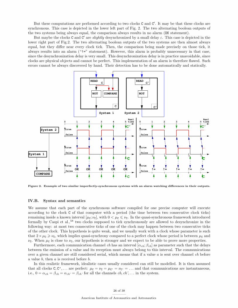
But these computations are performed according to two clocks C and C′. It may be that these clocks aresynchronous. This case is depicted in the lower left part of Fig. 2. The two alternating boolean outputs ofthe two systems being always equal, the comparison always results in no alarm (OK statement).

But maybe the clocks C and C′ are slightly desynchronized by a small delay ε. This case is depicted in thelower right part of Fig.2. The two alternating boolean outputs of the two systems are then almost alwaysequal, but they differ near every clock tick. Then, the comparison being made precisely on those tick, italways results into an alarm (“!=” statement). However, this alarm is probably unnecessary in that case,since the desynchronization delay is very small. This desynchronization delay is in practice unavoidable, sinceclocks are physical objects and cannot be perfect. This implementation of an alarm is therefore flawed. Sucherrors cannot be always discovered by hand. Their detection has to be done automatically and statically.

NOTNOT

READC

READ

C’

C’

C

COMPARE

System 1 System 2

!= != !=!= !=

0 2 3 4 51

C’true

false

C

true

false

C

true

false

Realtime

C

0 2 3 4 51

C’true

false

System 2

COMPARE

C

true

false

C

true

false

Realtime

C

OK OK OKOK OK

System 1ε ε εε ε

Figure 2. Example of two similar imperfectly-synchronous systems with an alarm watching differences in their outputs.

IV.B. Syntax and semantics

We assume that each part of the synchronous software compiled for one precise computer will executeaccording to the clock C of that computer with a period (the time between two consecutive clock ticks)remaining inside a known interval [µC; νC], with 0 < µC 6 νC. In the quasi-synchronous framework introducedformally by Caspi et al.,58 two clocks supposed to tick synchronously are allowed to desynchronize in thefollowing way: at most two consecutive ticks of one of the clock may happen between two consecutive ticksof the other clock. This hypothesis is quite weak, and we usually work with a clock whose parameter is suchthat 2×µC > νC, which implies quasi-synchrony compared to a perfect clock whose period is between µC andνC. When µC is close to νC, our hypothesis is stronger and we expect to be able to prove more properties.

Furthermore, each communication channel ch has an interval [αch;βch] as parameter such that the delaysbetween the emission of a value and its reception must always belong to this interval. The communicationsover a given channel are still considered serial, which means that if a value a is sent over channel ch beforea value b, then a is received before b.

In this realistic framework, idealistic cases usually considered can still be modelled. It is then assumedthat all clocks C, C’, . . . are perfect: µC = νC = µC’ = νC’ = . . . and that communications are instantaneous,i.e., 0 = αch = βch = αch’ = βch’ for all the channels ch, ch’, . . . in the system.

26 of 38


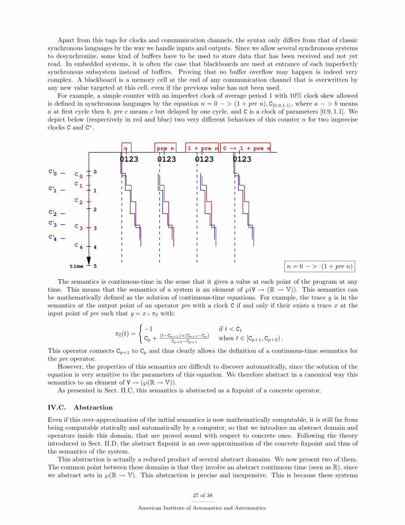
Apart from this tags for clocks and communication channels, the syntax only differs from that of classicsynchronous languages by the way we handle inputs and outputs. Since we allow several synchronous systemsto desynchronize, some kind of buffers have to be used to store data that has been received and not yetread. In embedded systems, it is often the case that blackboards are used at entrance of each imperfectlysynchronous subsystem instead of buffers. Proving that no buffer overflow may happen is indeed verycomplex. A blackboard is a memory cell at the end of any communication channel that is overwritten byany new value targeted at this cell, even if the previous value has not been used.

For example, a simple counter with an imperfect clock of average period 1 with 10% clock skew allowedis defined in synchronous languages by the equation n = 0 − > (1 + pre n), C[0.9,1.1], where a − > b meansa at first cycle then b, pre c means c but delayed by one cycle, and C is a clock of parameters [0.9, 1.1]. Wedepict below (respectively in red and blue) two very different behaviors of this counter n for two impreciseclocks C and C’.

n pre n 1 + pre n

0

1

3

4

5

2

C

C

C

C

C

0

1

2

3

4

C’1

C’0

C’2

C’3

4

0 3

0 −> 1 + pre n

12

time

0123 3321 10 0 2

C’

n = 0 − > (1 + pre n)

The semantics is continuous-time in the sense that it gives a value at each point of the program at anytime. This means that the semantics of a system is an element of ℘(V → (R → V)). This semantics canbe mathematically defined as the solution of continuous-time equations. For example, the trace y is in thesemantics at the output point of an operator pre with a clock C if and only if their exists a trace x at theinput point of pre such that y = x ◦ πC with:

πC(t) =

{−1 if t < C1

Cp + (t−Cp+1)×(Cp+1−Cp)Cp+2−Cp+1

when t ∈ [Cp+1, Cp+2) .

This operator connects Cp+1 to Cp and thus clearly allows the definition of a continuous-time semantics forthe pre operator.

However, the properties of this semantics are difficult to discover automatically, since the solution of theequation is very sensitive to the parameters of this equation. We therefore abstract in a canonical way thissemantics to an element of V→ (℘(R→ V)).

As presented in Sect. II.C, this semantics is abstracted as a fixpoint of a concrete operator.

IV.C. Abstraction

Even if this over-approximation of the initial semantics is now mathematically computable, it is still far frombeing computable statically and automatically by a computer, so that we introduce an abstract domain andoperators inside this domain, that are proved sound with respect to concrete ones. Following the theoryintroduced in Sect. II.D, the abstract fixpoint is an over-approximation of the concrete fixpoint and thus ofthe semantics of the system.

This abstraction is actually a reduced product of several abstract domains. We now present two of them.The common point between these domains is that they involve an abstract continuous time (seen as R), sincewe abstract sets in ℘(R → V). This abstraction is precise and inexpensive. This is because these systems

27 of 38


were in fact designed in a continuous world (through differential equations) in an environment (made ofspace and time) that is a continuous object. In addition, using a continuous-time semantics enables the useof very well-known mathematical theories about continuous numbers which are not so frequently used instatic analysis.

IV.D. Temporal abstract domains

IV.D.1. Abstract constraints

A first domain of abstract constraints59 abstracts ℘(R→ V) as conjunctive sets of universal and existentialconstraints. A universal constraint over a signal s ∈ R→ V is defined by a time interval [a; b] and a value x,and denoted ∀t ∈ [a; b] : s(t) = x. Its concretization is the set of signals in R→ V that take the value x duringthe whole time interval [a; b]. An existential constraint over a signal s is defined by a time interval [a; b] and avalue x, and denoted ∃t ∈ [a; b] : s(t) = x. Its concretization is the set of signals in R→ V that take the valuex at least once during the time interval [a; b]. For example, ∃t ∈ [0; 1] : s(t) = true ∧ ∃t ∈ [0; 1] : s(t) = falseis the abstraction of functions in R → B that change their boolean value at least once between t = 0 andt = 1.

The operators defined for usual operations in abstract domains (∪,∩) as well as the backward abstractoperators corresponding to synchronous language primitives (− >, pre, blackboard reading, etc.) are quiteprecise in this domain.

IV.D.2. Changes counting domain

A second domain of change counting60 was designed in order to deal automatically with reasoning on thestability and the variability of systems. The abstract properties (6 k, a� �b) and (> k, a� �b), for a, b ∈ R+

and k ∈ N, respectively mean that behaviors do not change their value more (respectively less) than k timesduring the time interval [a; b].

This domain is more precise for forward operators and defines a very precise reduced product with theabstract constraint domain.

An example of reduction is (with times a < b < c < d < e < f) when abstract an property u =(6 1, a� �e) interacts with the abstract properties v = ∃t ∈ [b; c] : s(t) = x and w = ∀t ∈ [d; f ] : s(t) = x.Then, if there is at least one value change between c and d, then there are actually at least two changes.Indeed, at some time t ∈ [c; d), the value has to be some y 6= x, since at time d it has to be x (by w) and itchanges at least once in [c, d]. Then, at some point t′ ∈ [b; c], the value has to be x (by v) which makes twovalue changes: one between t′ and t, and one between t and d. This is excluded by the stability propertyu. As a consequence, there is no value change between c and d and, since the value at time d is x anddoes not change, the value has to remain equal to x during whole time interval, which can be translatedinto ∀t ∈ [c; d] : s(t) = x. This constraint merges with the constraint ∀t ∈ [d; f ] : s(t) = x and yields∀t ∈ [c; f ] : s(t) = x.

IV.E. Application to redundant systems

It is often the case that similar (if not identical) systems run in parallel so that, in case one system hasa hardware failure, it is detected, either by the other similar systems or by a dedicated unit, and onlyredundant units keep performing the computation. The continuous-time semantics presented in this sectionhas been precisely designed to prove the properties of such systems.

Another classic embedded unit aims at treating sensor values. Sensor values are indeed very unstable andusually get stabilized by a synchronous system. The temporal abstract domains we introduced are preciseas well on the code for those systems.

A prototype static analyzer has been developed implementing the two temporal abstract domains pre-sented as well as other, less central domains. This prototype is independent from Astree (Sect. III) andThesee (Sect. VI).

The prototype analyzer was able to prove some temporal specification of redundant systems with a votingsystem deciding between them. Furthermore, when some property did not hold, looking at the remainingabstract set sometimes led to actual erroneous traces in altered implementations.

An example analysis involved the code used in industry as a test for such systems where clocks maydesynchronize and communication might be delayed. No hypothesis was given on the inputs of the studied

28 of 38


system but a specification was given for the output. We started several automatic analyses with severalhypothesis of value k as input stability, which led to discovering a constant value k0 such that:

• with an input stability of k0 milliseconds at least, the analyzer could prove the specification;

• with an input stability of 23 × k0 milliseconds or less, the analyzer could not prove the specification,

but in the computed abstract result, it was very easy to find (and this process could have been madeautomatic) a counter-example to the specification;

• with an input stability between 23 × k0 and k0, the analyzer could not prove the specification, while

the abstract result did not provide any obvious counter-example to the specification. It is thereforeunknown whether the specification holds in this case.

This result is very interesting since it demonstrates the necessity to stabilize input signals. But theanalyzer also provides a safe lower bound for this stabilization. In order for the analyzer to get closer tothe optimal stabilization, i.e., suggest a smaller minimal stability requirement, a new abstract domain maybe added in a modular way. Then, the properties proved by the previous domains would still be discoveredand, thanks to the added precision of the new domain, new properties may be discovered as well.

V. Verification of Target Programs

V.A. Verification requirements and compilation

In Sect. III, we addressed the verification of properties at the source level. However, source level code iscompiled into assembly code prior execution; thus, one may object that the verification performed at thesource level may not be convincing enough or may not be sound at all. Indeed, if the compiler itself containsa bug, then a C code which is correct according to the C semantics may be compiled into a target programwhich may crash abruptly. More generally, certification authorities usually require a precise definition ofthe properties which are validated (by verification or by testing) to be provided at the target level, whichrequires, at least, a good correspondence between the source and the target level to be established. As aconsequence, certification norms such as DO-178B61 often include target code verification requirements.

An alternative solution is to perform all verification tasks at the target level; yet, this approach is notadequate for all properties. It is well adapted for the verification of properties which can be defined reliablyonly at the compiled code level, such as worst case execution time properties.56 On the other hand, inferringprecise invariants in order to prove the absence of runtime errors is harder at assembly level, due to the loss ofcontrol and data structures induced by compilation. For instance, expressions are translated into sequencesof atomic, lower-level operations, which makes it harder for an analyzer to compute a precise invariant forthe whole operation: as an example, a conversion from integer data-type to floating-point data-type on aPowerPC target typically involves dozens of instructions, including bit masks and bit-field concatenations.

V.B. Semantics of compilation

When a direct target code level verification is too hard, other approaches can be applied, which allowsexploiting the results of a source level verification. Such approaches are based on a common pattern:either compilation should be correct (for some definition of correctness which we need to make explicit)or the verification of properties at the target level should be expected to fail. Thus, we need to formalizecompilation correctness first.

The abstract interpretation frameworks allows defining program transformations at the semantic level.62

Indeed, a program transformation usually aims at preserving some property of the semantics of the programbeing transformed, which we can define as an abstraction of the standard semantics. Then, the correctnessof the transformation boils down to a condition (such as equivalence) at this abstract level. Furthermore, thenotion of fixpoint transfer extends to this case, and allows a local definition of the transformation correctness.

In the case of compilation, and when the compiler performs no optimization, the target level abstractionshould forget about intermediate compilation steps; then, the correctness of the compilation can be expressedas a tight relation (such as the existence of a bi-simulation between the non-standard semantics, or as aninclusion between them). This relation is usually characterized by a relation between subsets of control pointsand variables of both the source and the target programs. A subtle yet important property is that this relation

29 of 38


can only be defined for valid source programs: for instance, if a C program violates the C semantics (e.g.,exhibits undefined behaviors), it is not possible to give a meaning for the compilation correctness in thatcase. When the compiler performs optimization, this simple definition can be extended, using more complexabstractions; for instance, dead variable elimination will cause some variables to be abstracted away at someprogram points.

We have formalized this framework.63 Given a compiler and compilation option, this framework allowsexpressing what property we should expect compilation to preserve, so that we can derive how to exploitthe results of source code verification so as to verify the target code.

V.C. Translation of invariants applied to target level verification

When the relation between program control points and variables in the source and compiled codes is known,and after invariants are computed for the source code, it is possible to translate automatically those invariantsinto invariants for the target code. When the compilation is indeed correct, the translated invariants aresound by construction. However, it is also possible to check the soundness of the translated invariantsindependently, which is much easier than inferring precise invariants for the compiled program directly. Whenthis independent check succeeds, the invariants are provably correct, independently from any assumption onthe correctness of the compiler or source code analyzer. Nevertheless, the fact that we expect the compilationto be correct is very important here, as this guides the translation of invariants.

This is the principle of proof carrying codes.64 This techniques generalizes to invariants computed byabstract interpretation-based static analyses of the source code.65

A disadvantage of such techniques is that not all kinds of invariants can be efficiently checked at assemblylevel; actually, case studies65 show that significant refinements are required in order to make the checking ofinvariants of the same kind as those produced by Astree succeed: indeed, checking invariants requires thesequence of instructions corresponding to each statement in the source code be analyzed precisely and partof the structure lost at compile time has to be reconstructed by the invariant checker.

V.D. Verification of compilation

An alternate solution consists in verifying the compilation itself. The principle of this approach is simple:we need to verify that the target code and the source code are correct in the sense stated above, i.e., thatthe tight relation between their abstract semantics holds. This can either be proved automatically after eachcompilation run (this technique is known as translation validation63,66,67) or only once, for the compiler itself(this technique is usually called compiler verification68). In both cases, the compilation is verified correct atsome level of abstraction in the sense of Sect. V.B. Moreover, the proof of equivalence is based on a set oflocal proofs: to prove the compilation correct, we only need to prove that each execution step in the sourcelevel is mapped into an equivalent step in the assembly and the converse (this is actually a consequence ofthe fixpoint transfer-based definition of compilation correctness).

When the compilation verification succeeds, it is possible to translate interesting properties to the targetcode, provided they can be established at the source level. This is the case for the absence of runtime errors,for instance. On the other hand, the correctness of compilation verification cannot usually be guaranteed ifthe source code cannot be proved correct: indeed, as we observed in Sect. V.B, the compilation correctnesscannot be defined in the case where the source program itself is not valid. Thus, the verification of thecompilation should follow the verification of the absence of runtime errors at the source level, e.g., using atool such as Astree.

Translation validation algorithms rely on automatic equivalence proof algorithms, which are either basedon model-checking66 or special purpose provers.63,67 These tools consider the compiler as a black box;thus, they apply to a range of compilers. On the other hand, compiler verification68 requires a manualformalization and proof of the compiler; thus, it needs to be done by the compiler designers; however, oncea compiler is verified, there is no need to run a (incomplete) verification tool to verify each compilation run.

VI. Verification of Parallel Programs

We now discuss on-going work on the verification of the absence of runtime errors in embedded parallelC software for realtime operating systems, with application to aeronautics.

30 of 38


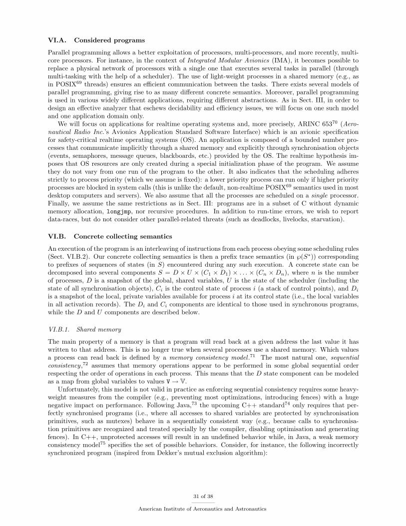
VI.A. Considered programs

Parallel programming allows a better exploitation of processors, multi-processors, and more recently, multi-core processors. For instance, in the context of Integrated Modular Avionics (IMA), it becomes possible toreplace a physical network of processors with a single one that executes several tasks in parallel (throughmulti-tasking with the help of a scheduler). The use of light-weight processes in a shared memory (e.g., asin POSIX69 threads) ensures an efficient communication between the tasks. There exists several models ofparallel programming, giving rise to as many different concrete semantics. Moreover, parallel programmingis used in various widely different applications, requiring different abstractions. As in Sect. III, in order todesign an effective analyzer that eschews decidability and efficiency issues, we will focus on one such modeland one application domain only.

We will focus on applications for realtime operating systems and, more precisely, ARINC 65370 (Aero-nautical Radio Inc.’s Avionics Application Standard Software Interface) which is an avionic specificationfor safety-critical realtime operating systems (OS). An application is composed of a bounded number pro-cesses that communicate implicitly through a shared memory and explicitly through synchronisation objects(events, semaphores, message queues, blackboards, etc.) provided by the OS. The realtime hypothesis im-poses that OS resources are only created during a special initialization phase of the program. We assumethey do not vary from one run of the program to the other. It also indicates that the scheduling adheresstrictly to process priority (which we assume is fixed): a lower priority process can run only if higher priorityprocesses are blocked in system calls (this is unlike the default, non-realtime POSIX69 semantics used in mostdesktop computers and servers). We also assume that all the processes are scheduled on a single processor.Finally, we assume the same restrictions as in Sect. III: programs are in a subset of C without dynamicmemory allocation, longjmp, nor recursive procedures. In addition to run-time errors, we wish to reportdata-races, but do not consider other parallel-related threats (such as deadlocks, livelocks, starvation).

VI.B. Concrete collecting semantics

An execution of the program is an interleaving of instructions from each process obeying some scheduling rules(Sect. VI.B.2). Our concrete collecting semantics is then a prefix trace semantics (in ℘(S∗)) correspondingto prefixes of sequences of states (in S) encountered during any such execution. A concrete state can bedecomposed into several components S = D × U × (C1 × D1) × . . . × (Cn × Dn), where n is the numberof processes, D is a snapshot of the global, shared variables, U is the state of the scheduler (including thestate of all synchronisation objects), Ci is the control state of process i (a stack of control points), and Di

is a snapshot of the local, private variables available for process i at its control state (i.e., the local variablesin all activation records). The Di and Ci components are identical to those used in synchronous programs,while the D and U components are described below.

VI.B.1. Shared memory

The main property of a memory is that a program will read back at a given address the last value it haswritten to that address. This is no longer true when several processes use a shared memory. Which valuesa process can read back is defined by a memory consistency model .71 The most natural one, sequentialconsistency ,72 assumes that memory operations appear to be performed in some global sequential orderrespecting the order of operations in each process. This means that the D state component can be modeledas a map from global variables to values V→ V.

Unfortunately, this model is not valid in practice as enforcing sequential consistency requires some heavy-weight measures from the compiler (e.g., preventing most optimizations, introducing fences) with a hugenegative impact on performance. Following Java,73 the upcoming C++ standard74 only requires that per-fectly synchronised programs (i.e., where all accesses to shared variables are protected by synchronisationprimitives, such as mutexes) behave in a sequentially consistent way (e.g., because calls to synchronisa-tion primitives are recognized and treated specially by the compiler, disabling optimisation and generatingfences). In C++, unprotected accesses will result in an undefined behavior while, in Java, a weak memoryconsistency model75 specifies the set of possible behaviors. Consider, for instance, the following incorrectlysynchronized program (inspired from Dekker’s mutual exclusion algorithm):

31 of 38


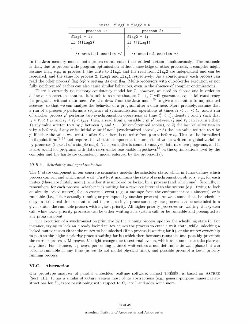
init: flag1 = flag2 = 0

process 1: process 2:

flag1 = 1; flag2 = 1;

if (!flag2) if (!flag1)

{ {/* critical section */ /* critical section */

In the Java memory model, both processes can enter their critical section simultaneously. The rationaleis that, due to process-wide program optimisation without knowledge of other processes, a compiler mightassume that, e.g., in process 1, the write to flag1 and the read from flag2 are independent and can bereordered, and the same for process 2, flag2 and flag1 respectively. As a consequence, each process canread the other process’ flag before setting its own flag. Multi-processors with out-of-order execution or notfully synchronized caches can also cause similar behaviors, even in the absence of compiler optimizations.

There is currently no memory consistency model for C; however, we need to choose one in order todefine our concrete semantics. It is safe to assume that, as C++, C will guarantee sequential consistencyfor programs without data-race. We also draw from the Java model75 to give a semantics to unprotectedaccesses, so that we can analyze the behavior of a program after a data-race. More precisely, assume thata run of a process p performs a sequence of synchronisation operations at times t1 < . . . < tn, and a runof another process p′ performs two synchronisation operations at time t′1 < t′2; denote i and j such thatti ≤ t′1 < ti+1 and tj ≤ t′2 < tj+1; then, a read from a variable v in p′ between t′1 and t′2 can return either:1) any value written to v by p between ti and tj+1 (unsynchronized access), or 2) the last value written tov by p before ti if any or its initial value if none (synchronized access), or 3) the last value written to v byp′ if either the value was written after t′1 or there is no write from p to v before ti. This can be formalizedin fixpoint form76,77 and requires the D state components to store sets of values written to global variablesby processes (instead of a simple map). This semantics is sound to analyze data-race-free programs, and itis also sound for programs with data-races under reasonable hypotheses75 on the optimizations used by thecompiler and the hardware consistency model enforced by the processor(s).

VI.B.2. Scheduling and synchronisation

The U state component in our concrete semantics models the scheduler state, which in turns defines whichprocess can run and which must wait. Firstly, it maintains the state of synchronisation objects, e.g., for eachmutex (there are finitely many), whether it is unlocked or locked by a process (and which one). Secondly, itremembers, for each process, whether it is waiting for a resource internal to the system (e.g., trying to lockan already locked mutex), for an external event (e.g., a message from the environment or a timeout), or isrunnable (i.e., either actually running or preempted by another process). As we assume that the schedulerobeys a strict real-time semantics and there is a single processor, only one process can be scheduled in agiven state: the runnable process with highest priority. All higher priority processes are waiting at a systemcall, while lower priority processes can be either waiting at a system call, or be runnable and preempted atany program point.

The execution of a synchronisation primitive by the running process updates the scheduling state U . Forinstance, trying to lock an already locked mutex causes the process to enter a wait state, while unlocking alocked mutex causes either the mutex to be unlocked (if no process is waiting for it), or the mutex ownershipto pass to the highest priority process waiting for it (which then becomes runnable, and possibly preemptsthe current process). Moreover, U might change due to external events, which we assume can take place atany time. For instance, a process performing a timed wait enters a non-deterministic wait phase but canbecome runnable at any time (as we do not model physical time), and possible preempt a lower priorityrunning process.

VI.C. Abstraction

Our prototype analyzer of parallel embedded realtime software, named Thesee, is based on Astree(Sect. III). It has a similar structure, reuses most of its abstractions (e.g., general-purpose numerical ab-stractions for Di, trace partitioning with respect to Ci, etc.) and adds some more.

32 of 38


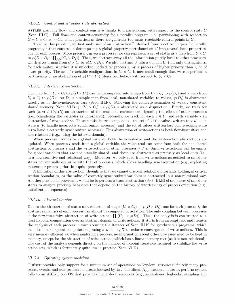
VI.C.1. Control and scheduler state abstraction

Astree was fully flow- and context-sensitive thanks to a partitioning with respect to the control state C(Sect. III.C). Full flow- and context-sensitivity for a parallel program, i.e., partitioning with respect toG = U × C1 × · · ·Cn, is not practical as there are generally too many reachable control points in G.

To solve this problem, we first make use of an abstraction,78 derived from proof techniques for parallelprograms,79 that consists in decomposing a global property partitioned on G into several local properties,one for each process. More precisely, given a process i, we can represent a set of states as a map from U ×Cito ℘(D×Di ×

∏j 6=i(Cj ×Dj)). Then, we abstract away all the information purely local to other processes,

which gives a map from U ×Ci to ℘(D×Di). We also abstract U into a domain Ui that only distinguishes,for each mutex, whether it is unlocked, locked by process i, by a process of higher priority than i, or oflower priority. The set of reachable configurations in Ui × Ci is now small enough that we can perform apartitioning of an abstraction of ℘(D ×Di) (described below) with respect to Ui × Ci.

VI.C.2. Interference abstraction

Our map from Ui ×Ci to ℘(D×Di) can be decomposed into a map from Ui ×Ci to ℘(Di) and a map fromUi × Ci to ℘(D). As Di is a simple map from local, non-shared variables to values, ℘(Di) is abstractedexactly as in the synchronous case (Sect. III.F). Following the concrete semantics of weakly consistentshared memory (Sect. VI.B.1), (Ui × Ci) → ℘(D) is abstracted as a disjunction. Firstly, we track foreach (u, c) ∈ (Ui, Ci) an abstraction of the reachable environments ignoring the effect of other processes(i.e., considering the variables as non-shared). Secondly, we track for each u ∈ Ui and each variable v anabstraction of write actions. These consist in two components: the set of all the values written to v while instate u (to handle incorrectly synchronized accesses), and the set of values written last before exiting stateu (to handle correctly synchronized accesses). This abstraction of write-actions is both flow-insensitive andnon-relational (e.g., using the interval domain).

When process i writes to a global variable, both the non-shared and the write-action abstractions areupdated. When process i reads from a global variable, the value read can come from both the non-sharedabstraction of process i and the write actions of other processes j 6= i. Such write actions will be emptyfor global variables that are not actually shared, and these are abstracted as precisely as local ones (i.e.,in a flow-sensitive and relational way). Moreover, we only read from write actions associated to schedulerstates not mutually exclusive with that of process i, which allows handling synchronization (e.g., exploitingmutexes or process priorities) quite precisely.

A limitation of this abstraction, though, is that we cannot discover relational invariants holding at criticalsection boundaries, as the value of correctly synchronized variables is abstracted in a non-relational way.Another possible improvement would be to perform a trace abstraction (Sect. III.E) of sequences of schedulerstates to analyze precisely behaviors that depend on the history of interleavings of process execution (e.g.,initialization sequences).

VI.C.3. Abstract iterator

Due to the abstraction of states as a collection of maps (Ui × Ci)→ ℘(D ×Di), one for each process i, theabstract semantics of each process can almost be computed in isolation. The only coupling between processesis the flow-insensitive abstraction of write actions

∏i(Ui → ℘(D)). Thus, the analysis is constructed as a

least fixpoint computation over an abstract domain of write actions. It starts from an empty set and iteratesthe analysis of each process in turn (reusing the iterator of Sect. III.K for synchronous programs, whichincludes inner fixpoint computations) using a widening

`to enforce convergence of write actions. This is

very memory efficient as, when analysing a process, no information about other processes need to be kept inmemory, except for the abstraction of write actions, which has a linear memory cost (as it is non-relational).The cost of the analysis depends directly on the number of fixpoint iterations required to stabilize the writeaction sets, which is fortunately quite low in practice (Sect. VI.D).

VI.C.4. Operating system modeling

Thesee provides only support for a minimum set of operations on low-level resources: finitely many pro-cesses, events, and non-recursive mutexes indexed by int identifiers. Applications, however, perform systemcalls to an ARINC 653 OS that provides higher-level resources (e.g., semaphores, logbooks, sampling and

33 of 38


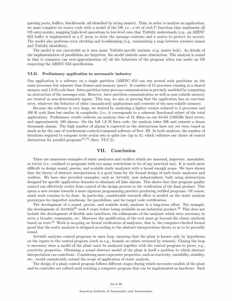
queuing ports, buffers, blackboards, all identified by string names). Thus, in order to analyze an application,we must complete its source code with a model of the OS, i.e., a set of stub C functions that implement allOS entry-points, mapping high-level operations to low-level ones that Thesee understands (e.g., an ARINC653 buffer is implemented as a C array to store the message contents and a mutex to protect its access).The model also performs error checking and bookkeeping (e.g., maintaining a map between resource namesand Thesee identifiers).

The model is not executable as it uses many Thesee-specific intrinsic (e.g, mutex lock). As details ofthe implementation of parallelism are forgotten, the model embeds some abstraction. The analysis is soundin that it computes (an over-approximation of) all the behaviors of the program when run under an OSrespecting the ARINC 653 specification.

VI.D. Preliminary application to aeronautic industry

Our application is a software on a single partition (ARINC 653 can run several such partitions on thesame processor but separate time frames and memory space). It consists of 15 processes running in a sharedmemory and 1.6 M code lines. Intra-partition inter-process communication is precisely modeled by computingan abstraction of the messages sent. However, inter-partition communication as well as non-volatile memoryare treated as non-deterministic inputs. This way, we aim at proving that the application has no run-timeerror, whatever the behavior of other (unanalyzed) applications and contents of the non-volatile memory.

Because the software is very large, we started by analyzing a lighter version reduced to 5 processes and100 K code lines but similar in complexity (i.e., it corresponds to a coherent functional subset of the totalapplication). Preliminary results indicate an analysis time of 1h 40mn on our 64-bit 2.66GHz Intel server,and approximately 100 alarms. On the full 1.6 M lines code, the analysis takes 50h and outputs a dozenthousands alarms. The high number of alarms is expected as the abstractions have not yet been tuned asmuch as for the case of synchronous control/command software of Sect. III. In both analyses, the number ofiterations required to compute write action sets is quite low (up to 4), which validates our choice of controlabstraction for parallel programs78,79 (Sect. VI.C.2).

VII. Conclusion

There are numerous examples of static analyzers and verifiers which are unsound, imprecise, unscalable,or trivial (i.e., confined to programs with too many restrictions to be of any practical use). It is much moredifficult to design sound, precise, and scalable static analyzers with a broad enough scope. We have shownthat the theory of abstract interpretation is a good basis for the formal design of such static analyzers andverifiers. We have also provided examples, such as Astree, now industrialized, built using abstractionsdesigned for specific application domains to eliminate all false alarms. This shows that that program qualitycontrol can effectively evolve from control of the design process to the verification of the final product. Thisopens a new avenue towards a more rigorous programming practice producing verified programs. Of course,much work remains to be done. In particular, considerable research effort is needed on the static analysisprototypes for imperfect synchrony, for parallelism, and for target code certification.

The development of a sound, precise, and scalable static analyzer is a long-term effort. For example,the development of Astree80 took 8 years before being available as an industrial product.38 This does notinclude the development of flexible user interfaces, the refinements of the analyzer which were necessary toserve a broader community, etc. Moreover the qualification of the tool must go beyond the classic methodsbased on tests.61 Work is on-going on formal verification of analyzers, that is, the computer-checked formalproof that the static analyzer is designed according to the abstract interpretation theory so as to be provablysound.

Astree analyzes control programs in open loop, meaning that the plant is known only by hypotheseson the inputs to the control program (such as e.g., bounds on values returned by sensors). Closing the loopis necessary since a model of the plant must be analyzed together with the control program to prove, e.g.,reactivity properties. Obtaining a sound abstract model of the plant is itself a problem to which abstractinterpretation can contribute. Considering more expressive properties, such as reactivity, variability, stability,etc., would considerably extend the scope of application of static analysis.

The design of a plant control program follows different stages during which successive models of the plantand its controller are refined until reaching a computer program that can be implemented on hardware. Such

34 of 38


refinements include physical limitations (such as coping with sensor or actuator failures), implementationdecisions (such as synchronous or asynchronous implementation on a mono- or multi-processor), etc. Waitingfor the final program to discover bugs by static analysis that have not been discovered by simulation ofthe various models is certainly useful but not completely efficient (in particular when functional bugs arediscovered by analysis of the origin of non-functional bugs such as overflows). Development methods canbe significantly improved to enhance safety, security, and reduce costs. In particular, static analyses ofthe different models would certainly speed up the development process and reduce the cost of bugs byearlier detection. Such static analysis tools are missing but can be developed. This raises the questionof high-level languages for describing models, which semantics is often vague or unrealistic (e.g., confusingreals and floats) and that of the translation of a specification from one model to another with differentsemantics. Automatically generating correct, efficient, and structured code would considerably help staticanalyzers (since dirty code is always more difficult to analyze) and static analyzers can definitely help in codegeneration (e.g., to choose the translation of real expressions to float so as to minimize rounding errors81).

Beyond safety concerns in embedded software, aeronautics is now confronted to security concerns withthe generalization of on-board Internet. Here again, security properties can be formalized and verified byabstract interpretation, which is a brand-new and rapidly developing domain of application.

In conclusion, static analysis can go well-beyond classic sequential programming languages and implicitspecifications towards the verification of complex computational models and systems. This is certainlynowadays a natural, challenging, and promising orientation for research in abstract interpretation.

References

1Cousot, P. and Cousot, R., “Abstract interpretation: a unified lattice model for static analysis of programs by constructionor approximation of fixpoints,” Conf. Rec. of the 4th Annual ACM SIGPLAN-SIGACT Symp. on Principles of ProgrammingLanguages (POPL’77), ACM Press (New York), Los Angeles, USA, Jan. 1977, pp. 238–252.

2Cousot, P., Cousot, R., Feret, J., Mauborgne, L., Mine, A., Monniaux, D., and Rival, X., “Varieties of Static Analyzers:A Comparison with Astree,” Proc. of the First Symp. on Theoretical Aspects of Software Engineering (TASE’07), edited byM. Hinchey, H. Jifeng, and J. Sanders, IEEE Comp. Soc. Press, Shanghai, China, 6–8 June 2007, pp. 3–17.

3Delmas, D. and Souyris, J., “Astree: from Research to Industry,” Proc. of the 14th Int. Static Analysis Symposium(SAS’07), edited by G. File and H. Riis-Nielson, Vol. 4634 of LNCS , Springer (Berlin), Kongens Lyngby, Denmark, 22–24 Aug.2007, pp. 437–451.

4Bouissou, O., Conquet, E., Cousot, P., Cousot, R., Feret, J., Goubault, E., Ghorbal, K., Lesens, D., Mauborgne, L.,Mine, A., Putot, S., Rival, X., and Turin, M., “Space Software Validation using Abstract Interpretation,” Proc. of the Int.Space System Engineering Conference, Data Systems In Aerospace (DASIA’09), ESA publications, Istanbul, Turkey, 26–29May 2009, pp. 1–7.

5Cousot, P., Methodes iteratives de construction et d’approximation de points fixes d’operateurs monotones sur un treillis,analyse semantique de programmes (in French), These d’Etat es sciences mathematiques, Universite scientifique et medicalede Grenoble, Grenoble, France, 21 Mar. 1978.

6Tarski, A., “A lattice theoretical fixpoint theorem and its applications,” Pacific Journal of Mathematics, Vol. 5, 1955,pp. 285–310.

7Cousot, P. and Cousot, R., “Systematic design of program analysis frameworks,” Conf. Rec. of the 6th Annual ACMSIGPLAN-SIGACT Symp. on Principles of Programming Languages (POPL’79), ACM Press (New York), San Antonio, USA,1979, pp. 269–282.

8Cousot, P. and Cousot, R., “Abstract Interpretation Frameworks,” Journal of Logic and Computation, Vol. 2, No. 4,Aug. 1992, pp. 511–547.

9Cousot, P. and Halbwachs, N., “Automatic discovery of linear restraints among variables of a program,” Conf. Rec. of the5th Annual ACM SIGPLAN-SIGACT Symp. on Principles of Programming Languages (POPL’78), ACM Press (New York),Tucson, USA, 1978, pp. 84–97.

10of Alexandria, E., “Elementa Geometriæ, Book XII, proposition 17,” fl. 300 BC.11Burstall, R. M., “Program proving as hand simulation with a little induction,” Information Processing, 1974, pp. 308–312.12Cousot, P. and Cousot, R., ““A la Burstall” intermittent assertions induction principles for proving inevitability properties

of programs,” Theoretical Computer Science, Vol. 120, 1993, pp. 123–155.13Floyd, R. W., “Assigning meanings to programs,” Proc. of the American Mathematical Society Symposia on Applied

Mathematics, Vol. 19, Providence, USA, 1967, pp. 19–32.14Cousot, P. and Cousot, R., “Sometime = Always + Recursion ≡ Always: on the equivalence of the intermittent and

invariant assertions methods for proving inevitability properties of programs,” Acta Informatica, Vol. 24, 1987, pp. 1–31.15Cousot, P., “Types as Abstract Interpretations,” Conf. Rec. of the 24th Annual ACM SIGPLAN-SIGACT Symp. on

Principles of Programming Languages (POPL’97), ACM Press (New York), Paris, France, Jan. 1997, pp. 316–331.16Besson, F., Cachera, D., Jensen, T., and Pichardie, D., “Certified Static Analysis by Abstract Interpretation,” Founda-

tions of Security Analysis and Design V, FOSAD 2007/2008/2009 Tutorial Lectures, Vol. 5705 of LNCS , Springer (Berlin),2009, pp. 223–257.

17Clarke, E., Grumberg, O., and Peled, D., Model Checking, MIT Press, Cambridge, 1999.

35 of 38


18Cousot, P., “Verification by Abstract Interpretation,” Proc. of the Int. Symp. on Verification – Theory & Practice –Honoring Zohar Manna’s 64th Birthday, edited by N. Dershowitz, Vol. 2772 of LNCS , Springer (Berlin), Taormina, Italy, 29June–4 July 2003, pp. 243–268.

19Cousot, P. and Cousot, R., “Comparing the Galois Connection and Widening/Narrowing Approaches to Abstract Inter-pretation,” Proc. of the 4th Int. Symp. on Programming Language Implementation and Logic Programming (PLILP’92), editedby M. Bruynooghe and M. Wirsing, Vol. 631 of LNCS , Springer (Berlin), Leuven, Belgium, 26–28 Aug. 1992, pp. 269–295.

20Cousot, P. and Cousot, R., “Static determination of dynamic properties of programs,” Proc. of the Second Int. Symp.on Programming (ISOP’76), Dunod, Paris, Paris, France, 1976, pp. 106–130.

21Bryant, R., “Graph-based algorithms for boolean function manipulation,” IEEE Trans. Computers, Vol. C-35, No. 8,1986.

22Jeannet, B. and Mine, A., “The Apron Numerical Abstract Domain Library,” http://apron.cri.ensmp.fr/library/.23Jeannet, B. and Mine, A., “Apron: A library of numerical abstract domains for static analysis,” Proc. of the 21st Int.

Conf. on Computer Aided Verification (CAV’09), Vol. 5643 of LNCS , Springer (Berlin), Grenoble, France, 26 June–2 July 22009, pp. 661–667.

24Granger, P., “Static Analysis of Arithmetical Congruences,” Int. J. Comput. Math., Vol. 30, No. 3 & 4, 1989, pp. 165–190.25Mine, A., “The Octagon Abstract Domain,” Higher-Order and Symbolic Computation, Vol. 19, 2006, pp. 31–100.26Feret, J., “Static Analysis of Digital Filters,” Proc. of the 13th European Symp. on Programming Languages and Systems

(ESOP’04), edited by D. Schmidt, Vol. 2986 of LNCS , Springer (Berlin), 27 Mar.–4 Apr. 2004, pp. 33–48.27Feret, J., “The Arithmetic-Geometric Progression Abstract Domain,” Proc. of the 6th Int. Conf. on Verification, Model

Checking and Abstract Interpretation (VMCAI’05), edited by R. Cousot, Vol. 3385 of LNCS , Springer (Berlin), Paris, France,17–19 Jan. 2005, pp. 42–58.

28Granger, P., “Static Analysis of Linear Congruence Equalities among Variables of a Program,” Proc. of the Int. JointConf. on Theory and Practice of Software Development (TAPSOFT’91), Volume 1 (CAAP’91), edited by S. Abramsky andT. Maibaum, Vol. 493 of LNCS , Springer (Berlin), Brighton, UK, 1991, pp. 169–192.

29Cousot, P., Cousot, R., Feret, J., Mauborgne, L., Mine, A., Monniaux, D., and Rival, X., “Combination of Abstractions inthe Astree Static Analyzer,” Proc. of the 11th Annual Asian Computing Science Conference (ASIAN’06), edited by M. Okadaand I. Satoh, Vol. 4435 of LNCS , Springer (Berlin), Tokyo, Japan, 6–8 Dec. 2006, pp. 272–300.

30Cousot, P., “Semantic Foundations of Program Analysis, invited chapter,” Program Flow Analysis: Theory and Appli-cations, edited by S. Muchnick and N. Jones, chap. 10, Prentice-Hall, Inc., Englewood Cliffs, 1981, pp. 303–342.

31Bourdoncle, F., “Abstract Interpretation by Dynamic Partitioning,” Journal of Functional Programming, Vol. 2, No. 4,1992, pp. 407–423.

32Giacobazzi, R., Ranzato, F., and Scozzari, F., “Making Abstract Interpretations Complete,” Journal of the Associationfor Computing Machinery, Vol. 47, No. 2, 2000, pp. 361–416.

33Cousot, P., Ganty, P., and Raskin, J.-F., “Fixpoint-Guided Abstraction Refinements,” Proc. of the 14th Int. StaticAnalysis Symposium (SAS’07), edited by G. File and H. Riis-Nielson, Vol. 4634 of LNCS , Springer (Berlin), Kongens Lyngby,Denmark, 22–24 Aug. 2007, pp. 333–348.

34Blanchet, B., Cousot, P., Cousot, R., Feret, J., Mauborgne, L., Mine, A., Monniaux, D., and Rival, X., “Design andImplementation of a Special-Purpose Static Program Analyzer for Safety-Critical Real-Time Embedded Software, invited chap-ter,” The Essence of Computation: Complexity, Analysis, Transformation. Essays Dedicated to Neil D. Jones, edited byT. Mogensen, D. Schmidt, and I. Sudborough, Vol. 2566 of LNCS , Springer (Berlin), 2002, pp. 85–108.

35Blanchet, B., Cousot, P., Cousot, R., Feret, J., Mauborgne, L., Mine, A., Monniaux, D., and Rival, X., “A StaticAnalyzer for Large Safety-Critical Software,” Proc. of the ACM SIGPLAN 2003 Conf. on Programming Language Design andImplementation (PLDI’03), ACM Press (New York), San Diego, USA, 7–14 June 2003, pp. 196–207.

36Cousot, P., Cousot, R., Feret, J., Mauborgne, L., Mine, A., Monniaux, D., and Rival, X., “The Astree analyser,” Proc.of the 14th European Symposium on Programming Languages and Systems (ESOP’05), edited by M. Sagiv, Vol. 3444 of LNCS ,Springer (Berlin), 2–10 Apr. 2005, pp. 21–30.

37Mauborgne, L., “Astree: Verification of Absence of Run-time error,” Building the Information Society, edited byP. Jacquart, chap. 4, Kluwer Academic Publishers, Dordrecht, 2004, pp. 385–392.

38AbsInt, Angewandte Informatik, “Astree Run-Time Error Analyzer,” http://www.absint.com/astree/.39Kastner, D., Wilhelm, S., Nenova, S., Cousot, P., Cousot, R., Feret, J., Mauborgne, L., Mine, A., and Rival, X., “Astree:

Proving the Absence of Rutime Errors,” Proc. of Embedded Real-Time Software and Systems (ERTS’10), Toulouse, France,May 2010, pp. 1–5, (to appear).

40ISO/IEC JTC1/SC22/WG14 Working Group, “C standard,” Tech. Rep. 1124, ISO & IEC, 2007.41Mauborgne, L. and Rival, X., “Trace Partitioning in Abstract Interpretation Based Static Analyzer,” Proc. of the 14th

European Symp. on Programming Languages and Systems (ESOP’05), edited by M. Sagiv, Vol. 3444 of LNCS , Springer(Berlin), Edinburg, UK, 4–8 Apr. 2005, pp. 5–20.

42Rival, X. and Mauborgne, L., “The trace partitioning abstract domain,” ACM Trans. Program. Lang. Syst., Vol. 29,No. 5, 2007.

43Mine, A., “Field-Sensitive Value Analysis of Embedded C Programs with Union Types and Pointer Arithmetics,” Proc.of the ACM SIGPLAN-SIGBED Conf. on Languages, Compilers, and Tools for Embedded Systems (LCTES’06), ACM Press(New York), June 2006, pp. 54–63.

44Moore, R. E., Interval Analysis, Prentice Hall, Englewood Cliffs N. J., USA, 1966.45IEEE Computer Society, “IEEE Standard for Binary Floating-Point Arithmetic,” Tech. rep., ANSI/IEEE Std. 745-1985,

1985.46Mine, A., “Relational Abstract Domains for the Detection of Floating-Point Run-Time Errors,” Proc. of the 13th European

Symp. on Programming Languages and Systems (ESOP’04), edited by D. Schmidt, Vol. 2986 of LNCS , Springer (Berlin), 27Mar.27–4 Apr. 2004, pp. 3–17.

36 of 38


47Mine, A., Weakly Relational Numerical Abstract Domains, These de doctorat en informatique, Ecole polytechnique,Palaiseau, France, 6 Dec. 2004.

48Goubault, E., “Static analyses of floating-point operations,” Proc. of the 8th Int. Static Analysis Symposium (SAS’01),Vol. 2126 of LNCS , Springer (Berlin), 2001, pp. 234–259.

49Mine, A., “The Octagon Abstract Domain,” Proc. of the Analysis, Slicing and Transformation Workshop (AST’01),IEEE Computer Society Press (Los Alamitos), Oct. 2001, pp. 310–319.

50Larsen, K., Larsson, F., Pettersson, P., and Yi, W., “Efficient Verification of Real-Time Systems: Compact Data Structureand State-Space Reduction,” Proc. of the 18th IEEE Real-Time Systems Symp. (RTSS’97), IEEE CS Press, 1997, pp. 14–24.

51Bryant, R. E., “Graph-Based Algorithms for Boolean Function Manipulation,” IEEE Transactions on Computers, Vol. 35,1986, pp. 677–691.

52Feret, J., “Numerical Abstract Domains for Digital Filters,” Proc. of the First Int. Workshop on Numerical & SymbolicAbstract Domains (NSAD’05), Maison Des Polytechniciens, Paris, France, 21 Jan. 2005.

53Monniaux, D., “The parallel implementation of the Astree static analyzer,” Proc. of the 3rd Asian Symp. on Program-ming Languages and Systems (APLAS’05), Vol. 3780 of LNCS , Springer (Berlin), 2005, pp. 86–96.

54Bourdoncle, F., “Efficient Chaotic Iteration Strategies with Widenings,” Proc. of the Int. Conf. on Formal Methods inProgramming and their Applications (FMPA’93), Vol. 735 of LNCS , Springer (Berlin), 1993, pp. 128–14.

55Esterel Technologies, “SCADE SuiteTM, The Standard for the Development of Safety-Critical Embedded Software in theAvionics Industry,” http://www.esterel-technologies.com/.

56Heckmann, R. and Ferdinand, C., “Worst-Case Execution Time Prediction by Static Program Analysis,” Proc. of the18th Int. Parallel and Distributed Processing Symposium (IPDPS’04), IEEE Computer Society, 2004, pp. 26–30.

57Ginosar, R., “Fourteen Ways to Fool Your Synchronizer,” Proc. of the 9th International Symposium on AsynchronousCircuits and Systems (ASYNC’03), 2003, pp. 89–97.

58Caspi, P., Mazuet, C., and Paligot, N. R., “About the Design of Distributed Control Systems: The Quasi-SynchronousApproach,” 20th International Conference on Computer Safety, Reliability and Security (SAFECOMP 2001), edited by U. Vo-ges, Vol. 2187 of LNCS , Springer (Berlin), Budapest, Hungary, Sept. 2001, pp. 215–226.

59Bertrane, J., “Static analysis by abstract interpretation of the quasi-synchronous composition of synchronous programs,”Proc. of the 6th Int. Conf. on Verification, Model Checking and Abstract Interpretation (VMCAI’05), edited by R. Cousot,Vol. 3385 of LNCS , Springer (Berlin), Paris, France, 17–19 Jan. 2005, pp. 97–112.

60Bertrane, J., “Proving the Properties of Communicating Imperfectly-Clocked Synchronous Systems,” Proc. of the 13thInt. Static Analysis Symposium (SAS’06), edited by K. Yi, Vol. 4134 of LNCS , Springer (Berlin), Seoul, Korea, 29–31 Aug.2006, pp. 370–386.

61Technical Commission on Aviation, R., “DO-178B,” Tech. rep., Software Considerations in Airborne Systems and Equip-ment Certification, 1999.

62Cousot, P. and Cousot, R., “Systematic Design of Program Transformation Frameworks by Abstract Interpretation,”Conf. Rec. of the 29th Annual ACM SIGPLAN-SIGACT Symp. on Principles of Programming Languages (POPL’02), ACMPress (New York), Portland, USA, Jan. 2002, pp. 178–190.

63Rival, X., “Symbolic transfer functions-based approaches to certified compilation,” Conf. Rec. of the 31st Annual ACMSIGPLAN-SIGACT Symp. on Principles of Programming Languages (POPL’04), ACM Press (New York), Venice, Italy, Jan.2004, pp. 1–13.

64Necula, G. C., “Proof-Carrying Code,” Conf. Rec. of the 24th Annual ACM SIGPLAN-SIGACT Symp. on Principlesof Programming Langauges (POPL’97), ACM Press (New York), Paris, France, Jan. 1997, pp. 106–119.

65Rival, X., “Abstract Interpretation-based Certification of Assembly Code,” Proc. of the 4th Int. Conf. on Verification,Model Checking and Abstract Interpretation (VMCAI’03), Vol. 2575 of LNCS , Springer (Berlin), New York, USA, Jan. 2003,pp. 41–55.

66Pnueli, A., Shtrichman, O., and Siegel, M., “Translation Validation for Synchronous Languages,” Proc. of the 25th Int.Coll. on Automata, Languages and Programming (ICALP’98), Vol. 1443 of LNCS , Springer (Berlin), Aalborg, Denmark, Jul.1998, pp. 235–246.

67Necula, G. C., “Translation Validation for an Optimizing Compiler,” Proc. of the Conf. on Programming LanguageDesign and Implementation (PLDI’00), ACM Press (New York), Vancouver, Canada, June 2000, pp. 83–94.

68Leroy, X., “Formal certification of a compiler back-end or: programming a compiler with a proof assistant,” Conf. Rec.of the 33rd Annual ACM SIGPLAN-SIGACT Symp. on Principles of Programming Languages (POPL’06), ACM Press (NewYork), Charleston, USA, 2006, pp. 42–54.

69IEEE and The Open Group, “Portable Operating System Interface (POSIX),” http://www.opengroup.org, http://

standards.ieee.org.70Aeronautical Radio, Inc. (ARINC), “ARINC 653,” http://www.arinc.com/.71Saraswat, V., Jagadeesan, R., Michael, M., and von Praun, C., “A theory of memory models,” Proc. of the 12th ACM

SIGPLAN Symp. on Principles and Practice of Parallel Programming (PPOPP’07), ACM Press (New York), San Jose, USA,Mar. 2007, pp. 161–172.

72Lamport, L., “How to make a multiprocessor computer that correctly executes multiprocess programs,” IEEE Transac-tions on Computers, Vol. 28, Sept. 1979, pp. 690–691.

73Gosling, J., Joy, B., Steele, G., and Bracha, G., The Java language specification, third edition, Addison Wesley, 2005.74ISO/IEC JTC1/SC22/WG21 Working Group, “Working draft, standard for programming language C++,” Tech. Rep.

3035, ISO & IEC, 2010.75Manson, J., Pugh, W., and Adve, S. V., “The Java memory model,” Conf. Rec. of the 32nd Annual ACM SIGPLAN-

SIGACT Symp. on Principles of Programming Languages (POPL’05), ACM Press (New York), Long Beach, USA, 2005, pp.378–391.

37 of 38


76Ferrara, P., “Static analysis via abstract interpretation of the happens-before memory model,” Proc. of the Second Int.Conf. on Tests and Proofs (TAP’08), Vol. 4966 of LNCS , Springer (Berlin), 2008, pp. 116–133.

77Ferrara, P., Static analysis via abstract interpretation of multithreaded programs, Ph.D. thesis, Ecole Polytechnique,Palaiseau, France, May 2009.

78Cousot, P. and Cousot, R., Invariance proof methods and analysis techniques for parallel programs, chap. 12, Macmillan,New York, USA, 1984, pp. 243–271.

79Owicki, S. and Gries, D., “An axiomatic proof technique for parallel programs I,” Acta Informatica, Vol. 6, No. 4, Dec.1976, pp. 319–340.

80Cousot, P., Cousot, R., Feret, J., Mauborgne, L., Mine, A., and Rival, X., “The Astree static analyzer,” www.astree.

ens.fr and www.absint.com/astree/.81Martel, M., “Enhancing the implementation of mathematical formulas for fixed-point and floating-point arithmetics,”

Formal Methods in System Design, Vol. 35, No. 3, Dec. 2009, pp. 265–278.

38 of 38


Documents

Static Analysis and Veri cation of Aerospace Software by