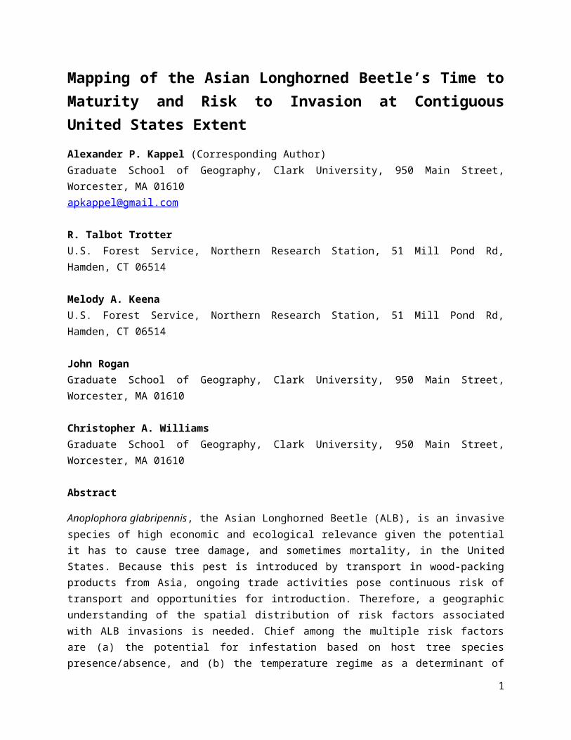
Mapping of the Asian Longhorned Beetle’s Time to Maturity and Risk to Invasion at Contiguous United States Extent

Alexander P. Kappel (Corresponding Author)Graduate School of Geography, Clark University, 950 Main Street, Worcester, MA 01610apkappel@gmail.com

R. Talbot TrotterU.S. Forest Service, Northern Research Station, 51 Mill Pond Rd, Hamden, CT 06514

Melody A. KeenaU.S. Forest Service, Northern Research Station, 51 Mill Pond Rd, Hamden, CT 06514

John RoganGraduate School of Geography, Clark University, 950 Main Street, Worcester, MA 01610

Christopher A. WilliamsGraduate School of Geography, Clark University, 950 Main Street, Worcester, MA 01610

Abstract

Anoplophora glabripennis, the Asian Longhorned Beetle (ALB), is an invasive species of high economic and ecological relevance given the potential it has to cause tree damage, and sometimes mortality, in the United States. Because this pest is introduced by transport in wood-packing products from Asia, ongoing trade activities pose continuous risk of transport and opportunities for introduction. Therefore, a geographic understanding of the spatial distribution of risk factors associated with ALB invasions is needed. Chief among the multiple risk factors are (a) the potential for infestation based on host tree species presence/absence, and (b) the temperature regime as a determinant of ALB’s growth time to maturity. This study uses an empirical model of ALB’s time to maturity as a function of temperature, along with a model of heat transfer in the wood of the host and spatial data describing host species presence/absence data, to produce a map of risk factors across the conterminous United States to define potential for ALB infestation and relative threat of impact. Results show that the region with greatest risk of ALB infestation is the eastern half of the country, with lower risk across most of the western half due to low abundance of host species, less urban area, and prevalence of cold, high elevations. Risk is high in southeastern states primarily because of temperature, while risk is high in northeastern and northern central states because of high abundance of host species.

Keywords

Asian Longhorned Beetle, Anoplophora glabripennis, Invasion, Colonization, Risk, Maturity, United States, Modeling, Degree Days, Temperature, Host Species, Distribution, Instar

1

5. Supporting Information

5.1 Supporting Figures

Figure 1- A comparison of the two risk scenarios. Green areas contain species known to be at risk to ALB given a past observed vulnerability. These green areas define the spatial extent of the species scenario. Red areas contain species that have not yet been observed as vulnerable but that may be at risk due to membership in a genus which already contains other vulnerable species. These red areas plus the green areas define the spatial extent of the genus scenario.

2

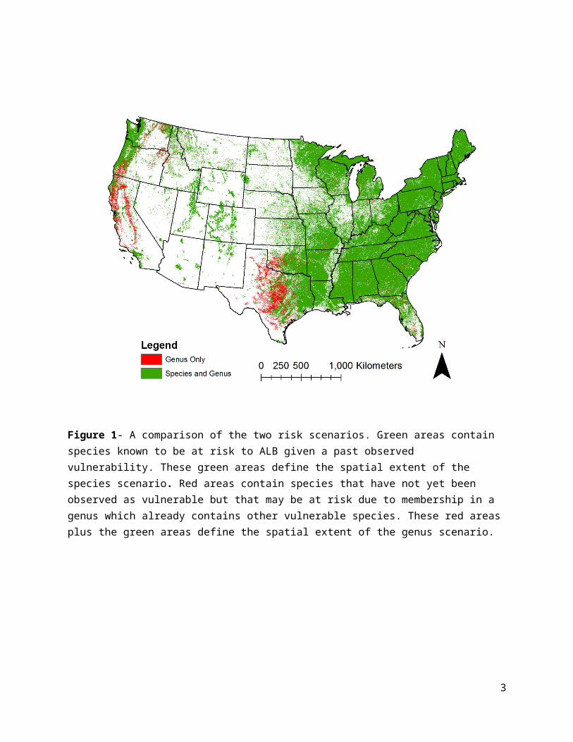
Figure 2- ALB years to maturity for viable host area defined by urban areas and genus scenario risk extent.

3

Figure 3- The percent timber basal area at risk to ALB given a genus scenario risk extent.

4

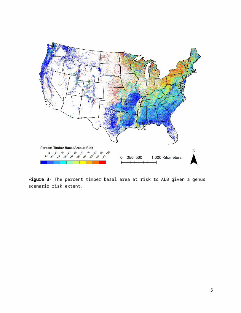
Figure 4- The mean basal area of vulnerable timber, given a genus scenario risk extent.

5

5.2 Supporting Tables

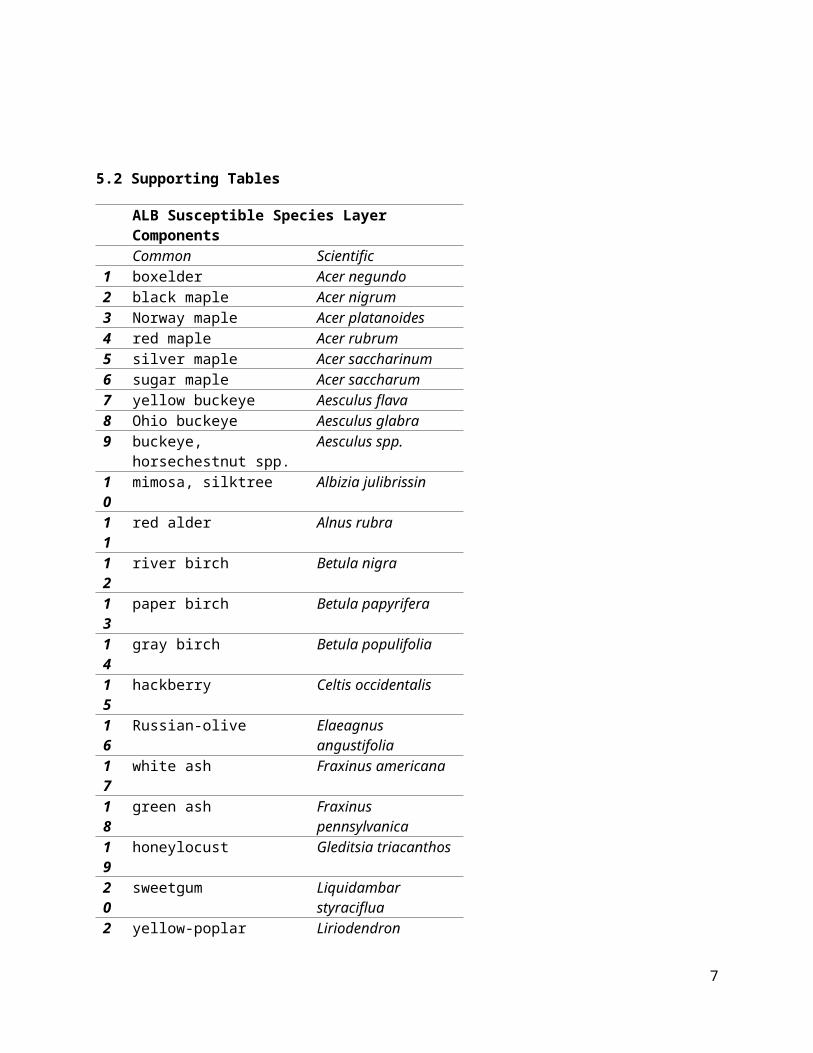
ALB Susceptible Species Layer ComponentsCommon Scientific

1 boxelder Acer negundo2 black maple Acer nigrum3 Norway maple Acer platanoides4 red maple Acer rubrum5 silver maple Acer saccharinum6 sugar maple Acer saccharum7 yellow buckeye Aesculus flava8 Ohio buckeye Aesculus glabra9 buckeye, horsechestnut spp. Aesculus spp.10

mimosa, silktree Albizia julibrissin

11

red alder Alnus rubra

12

river birch Betula nigra

13

paper birch Betula papyrifera

14

gray birch Betula populifolia

15

hackberry Celtis occidentalis

16

Russian-olive Elaeagnus angustifolia

17

white ash Fraxinus americana

18

green ash Fraxinus pennsylvanica

19

honeylocust Gleditsia triacanthos

20

sweetgum Liquidambar styraciflua

21

yellow-poplar Liriodendron tulipifera

22

white mulberry Morus alba

23

eastern hophornbeam Ostrya virginiana

24

American sycamore Platanus occidentalis

25

black cottonwood Populus balsamifera

26

silver poplar Populus alba

6

27

eastern cottonwood Populus deltoides

28

quaking aspen Populus tremuloides

29

Lombardy poplar Populus nigra

30

peach Prunus persica

31

black locust Robinia pseudoacacia

32

white willow Salix alba

33

black willow Salix nigra

34

European mountain-ash Sorbus aucuparia

35

American basswood Tilia americana

36

white basswood Tilia americana

37

Carolina basswood Tilia americana

38

American elm Ulmus americana

39

Siberian elm Ulmus pumila

Table 1- List of tree species composing the species scenario risk extent. This list is made up of known susceptible species as referenced by Meng et al. (2015).

7

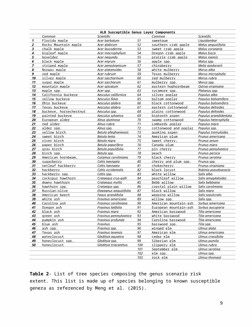
ALB Susceptible Genus Layer ComponentsCommon Scientific Common Scientific

1 Florida maple Acer barbatum 51 sweetgum Liquidambar styraciflua2 Rocky Mountain maple Acer glabrum 52 southern crab apple Malus angustifolia3 chalk maple Acer leucoderme 53 sweet crab apple Malus coronaria4 bigleaf maple Acer macrophyllum 54 Oregon crab apple Malus fusca5 boxelder Acer negundo 55 prairie crab apple Malus ioensis6 black maple Acer nigrum 56 apple spp. Malus spp.7 striped maple Acer pensylvanicum 57 chinaberry Melia azedarach8 Norway maple Acer platanoides 58 white mulberry Morus alba9 red maple Acer rubrum 59 Texas mulberry Morus microphylla10 silver maple Acer saccharinum 60 red mulberry Morus rubra11 sugar maple Acer saccharum 61 mulberry spp. Morus spp.12 mountain maple Acer spicatum 62 eastern hophornbeam Ostrya virginiana13 maple spp. Acer spp. 63 sycamore spp. Platanus spp.14 California buckeye Aesculus californica 64 silver poplar Populus alba15 yellow buckeye Aesculus flava 65 balsam poplar Populus balsamifera16 Ohio buckeye Aesculus glabra 66 black cottonwood Populus balsamifera17 Texas buckeye Aesculus glabra 67 eastern cottonwood Populus deltoides18 buckeye, horsechestnut spp. Aesculus spp. 68 plains cottonwood Populus deltoides19 painted buckeye Aesculus sylvatica 69 bigtooth aspen Populus grandidentata20 European alder Alnus glutinosa 70 swamp cottonwood Populus heterophylla21 red alder Alnus rubra 71 Lombardy poplar Populus nigra22 alder spp. Alnus spp. 72 cottonwood and poplar spp. Populus spp.23 yellow birch Betula alleghaniensis 73 quaking aspen Populus tremuloides24 sweet birch Betula lenta 74 American plum Prunus americana25 river birch Betula nigra 75 sweet cherry, domesticated Prunus avium26 paper birch Betula papyrifera 76 Canada plum Prunus nigra27 gray birch Betula populifolia 77 pin cherry Prunus pensylvanica28 birch spp. Betula spp. 78 peach Prunus persica29 American hornbeam, musclewood Carpinus caroliniana 79 black cherry Prunus serotina30 sugarberry Celtis laevigata 80 cherry and plum spp. Prunus spp.31 netleaf hackberry Celtis laevigata 81 chokecherry Prunus virginiana32 hackberry Celtis occidentalis 82 black locust Robinia pseudoacacia33 hackberry spp. Celtis spp. 83 white willow Salix alba34 cockspur hawthorn Crataegus crus-galli 84 peachleaf willow Salix amygdaloides35 downy hawthorn Crataegus mollis 85 Bebb willow Salix bebbiana36 hawthorn spp. Crataegus spp. 86 coastal plain willow Salix caroliniana37 Russian-olive Elaeagnus angustifolia 87 black willow Salix nigra38 American beech Fagus grandifolia 88 weeping willow Salix sepulcralis39 white ash Fraxinus americana 89 willow spp. Salix spp.40 Carolina ash Fraxinus caroliniana 90 American mountain-ash Sorbus americana41 Oregon ash Fraxinus latifolia 91 European mountain-ash Sorbus aucuparia42 black ash Fraxinus nigra 92 American basswood Tilia americana43 green ash Fraxinus pennsylvanica 93 white basswood Tilia americana44 pumpkin ash Fraxinus profunda 94 Carolina basswood Tilia americana45 blue ash Fraxinus quadrangulata 95 basswood spp. Tilia spp.46 ash spp. Fraxinus spp. 96 winged elm Ulmus alata47 Texas ash Fraxinus texensis 97 American elm Ulmus americana48 waterlocust Gleditsia aquatica 98 cedar elm Ulmus crassifolia49 honeylocust spp. Gleditsia spp. 99 Siberian elm Ulmus pumila50 honeylocust Gleditsia triacanthos 100 slippery elm Ulmus rubra

101 September elm Ulmus serotina102 elm spp. Ulmus spp.103 rock elm Ulmus thomasii

Table 2- List of tree species composing the genus scenario risk extent. This list is made up of species belonging to known susceptible genera as referenced by Meng et al. (2015).

8

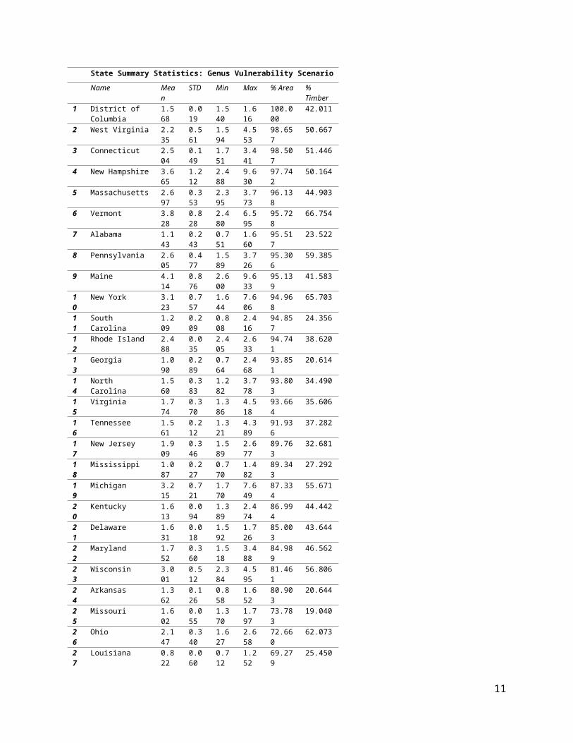
State Summary Statistics: Genus Vulnerability ScenarioName Mea

nSTD Min Max % Area %

Timber1 District of Columbia 1.568 0.01

91.540 1.61

6100.000 42.011

2 West Virginia 2.235 0.561

1.594 4.553

98.657 50.667

3 Connecticut 2.504 0.149

1.751 3.441

98.507 51.446

4 New Hampshire 3.665 1.212

2.488 9.630

97.742 50.164

5 Massachusetts 2.697 0.353

2.395 3.773

96.138 44.903

6 Vermont 3.828 0.828

2.480 6.595

95.728 66.754

7 Alabama 1.143 0.243

0.751 1.660

95.517 23.522

8 Pennsylvania 2.605 0.477

1.589 3.726

95.306 59.385

9 Maine 4.114 0.876

2.600 9.633

95.139 41.583

10

New York 3.123 0.757

1.644 7.606

94.968 65.703

11

South Carolina 1.209 0.209

0.808 2.416

94.857 24.356

12

Rhode Island 2.488 0.035

2.405 2.633

94.741 38.620

13

Georgia 1.090 0.289

0.764 2.468

93.851 20.614

14

North Carolina 1.560 0.383

1.282 3.778

93.803 34.490

15

Virginia 1.774 0.370

1.386 4.518

93.664 35.606

16

Tennessee 1.561 0.212

1.321 4.389

91.936 37.282

17

New Jersey 1.909 0.346

1.589 2.677

89.763 32.681

18

Mississippi 1.087 0.227

0.770 1.482

89.343 27.292

19

Michigan 3.215 0.721

1.770 7.649

87.334 55.671

20

Kentucky 1.613 0.094

1.389 2.474

86.994 44.442

21

Delaware 1.631 0.018

1.592 1.726

85.003 43.644

22

Maryland 1.752 0.360

1.518 3.488

84.989 46.562

23

Wisconsin 3.001 0.512

2.384 4.595

81.461 56.806

24

Arkansas 1.362 0.126

0.858 1.652

80.903 20.644

25

Missouri 1.602 0.055

1.370 1.797

73.783 19.040

26

Ohio 2.147 0.340

1.627 2.658

72.660 62.073

27

Louisiana 0.822 0.060

0.712 1.252

69.279 25.450

28

Indiana 1.852 0.307

1.512 2.480

61.043 56.223

29

Oklahoma 1.348 0.090

0.866 1.704

59.610 21.283

30

Minnesota 3.414 0.721

2.438 6.622

59.071 52.436

3 Florida 0.736 0.05 0.592 0.84 58.789 9.217

9

1 4 732

Washington 4.883 1.597

1.723 9.674

44.309 6.506

33

Illinois 1.769 0.294

1.471 2.504

44.110 46.924

34

Texas 0.846 0.149

0.619 1.693

39.372 12.463

35

Iowa 2.098 0.347

1.649 2.627

31.906 54.539

36

Oregon 4.329 1.475

1.778 9.800

30.774 4.590

37

Kansas 1.575 0.055

1.400 2.373

29.231 57.447

38

California 2.309 1.365

0.619 9.986

22.806 1.445

39

Idaho 5.367 1.769

1.751 9.677

21.704 2.295

40

Nebraska 2.058 0.369

1.633 2.773

17.156 49.372

41

Colorado 5.827 2.190

1.586 9.677

16.025 12.498

42

Montana 5.611 2.207

2.493 9.668

12.273 2.729

43

Utah 5.281 2.000

0.803 9.666

12.138 6.559

44

North Dakota 3.061 0.488

2.490 4.562

11.286 67.991

45

Wyoming 6.242 2.089

2.485 9.677

10.051 5.704

46

South Dakota 3.017 1.217

1.740 8.594

9.579 14.779

47

New Mexico 4.490 2.348

0.822 9.644

4.431 1.697

48

Nevada 4.651 2.155

0.627 9.663

3.626 1.315

49

Arizona 2.678 2.447

0.619 9.636

3.602 1.190

Table 3- Summary statistics for states and District of Columbia, sorted by percent area at risk, given the genus scenario. ‘% Area’ refers to the vulnerable grid cell percent of a state’s area and ‘% Timber’ refers to the vulnerable percent of a state’s timber basal area. Mean, standard deviation, min, and max, refer to time to maturity.

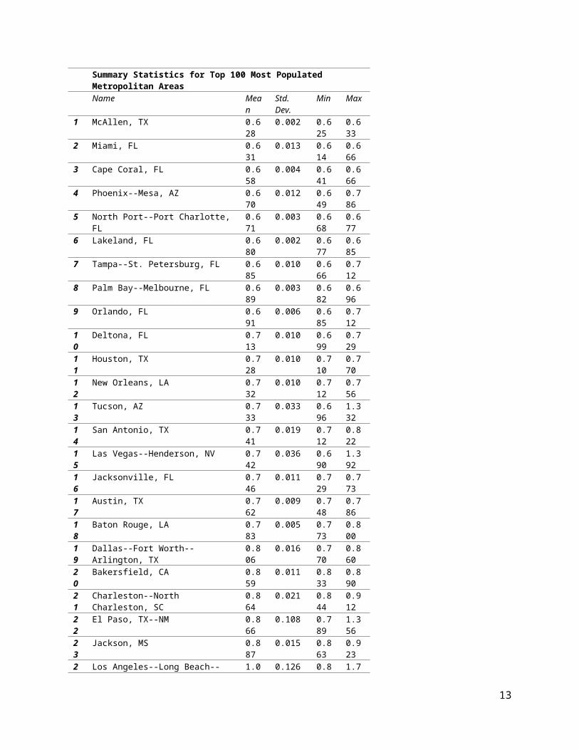
Summary Statistics for Top 100 Most Populated Metropolitan AreasName Mea

nStd. Dev.

Min Max

1 McAllen, TX 0.628 0.002 0.625

0.633

2 Miami, FL 0.631 0.013 0.614

0.666

3 Cape Coral, FL 0.658 0.004 0.641

0.666

4 Phoenix--Mesa, AZ 0.670 0.012 0.649

0.786

5 North Port--Port Charlotte, FL 0.671 0.003 0.668

0.677

6 Lakeland, FL 0.680 0.002 0.677

0.685

10

7 Tampa--St. Petersburg, FL 0.685 0.010 0.666

0.712

8 Palm Bay--Melbourne, FL 0.689 0.003 0.682

0.696

9 Orlando, FL 0.691 0.006 0.685

0.712

10

Deltona, FL 0.713 0.010 0.699

0.729

11

Houston, TX 0.728 0.010 0.710

0.770

12

New Orleans, LA 0.732 0.010 0.712

0.756

13

Tucson, AZ 0.733 0.033 0.696

1.332

14

San Antonio, TX 0.741 0.019 0.712

0.822

15

Las Vegas--Henderson, NV 0.742 0.036 0.690

1.392

16

Jacksonville, FL 0.746 0.011 0.729

0.773

17

Austin, TX 0.762 0.009 0.748

0.786

18

Baton Rouge, LA 0.783 0.005 0.773

0.800

19

Dallas--Fort Worth--Arlington, TX 0.806 0.016 0.770

0.860

20

Bakersfield, CA 0.859 0.011 0.833

0.890

21

Charleston--North Charleston, SC 0.864 0.021 0.844

0.912

22

El Paso, TX--NM 0.866 0.108 0.789

1.356

23

Jackson, MS 0.887 0.015 0.863

0.923

24

Los Angeles--Long Beach--Anaheim, CA 1.020 0.126 0.838

1.740

25

Riverside--San Bernardino, CA 1.037 0.142 0.896

1.753

26

Fresno, CA 1.144 0.118 0.937

1.280

27

San Diego, CA 1.216 0.121 0.981

1.666

28

Augusta-Richmond County, GA--SC 1.222 0.055 0.989

1.310

29

Columbia, SC 1.265 0.087 0.921

1.356

30

Birmingham, AL 1.300 0.023 1.258

1.367

31

Little Rock, AR 1.316 0.011 1.290

1.345

32

Memphis, TN--MS--AR 1.342 0.013 1.321

1.370

33

Stockton, CA 1.354 0.002 1.351

1.359

34

Oklahoma City, OK 1.364 0.009 1.342

1.384

35

Sacramento, CA 1.372 0.042 1.348

1.592

36

Atlanta, GA 1.378 0.023 1.345

1.526

3 Greenville, SC 1.380 0.008 1.36 1.488

11

7 238

Tulsa, OK 1.381 0.003 1.373

1.392

39

Virginia Beach, VA 1.398 0.011 1.386

1.507

40

Raleigh, NC 1.400 0.029 1.375

1.507

41

Charlotte, NC--SC 1.408 0.054 1.367

1.573

42

Chattanooga, TN--GA 1.423 0.064 1.381

1.647

43

Durham, NC 1.451 0.042 1.392

1.523

44

Nashville-Davidson, TN 1.492 0.047 1.395

1.556

45

Wichita, KS 1.516 0.007 1.504

1.540

46

Greensboro, NC 1.518 0.009 1.477

1.537

47

Winston-Salem, NC 1.540 0.017 1.488

1.589

48

Knoxville, TN 1.540 0.021 1.474

1.600

49

Richmond, VA 1.545 0.021 1.490

1.586

50

St. Louis, MO--IL 1.553 0.019 1.515

1.597

Table 4- Summary statistics for top 100 (by population) metropolitan areas, sorted by mean time to maturity.

Summary Statistics for Top 100 Most Populated Metropolitan Areas (Continued)Name Mean Std. Dev. Min Max

51 Louisville/Jefferson County, KY--IN 1.562 0.033 1.512 1.65252 Kansas City, MO--KS 1.580 0.016 1.545 1.63853 Baltimore, MD 1.609 0.029 1.559 1.72354 Oxnard, CA 1.610 0.112 1.422 1.97855 Washington, DC--VA--MD 1.620 0.035 1.540 1.70456 Albuquerque, NM 1.627 0.046 1.584 2.48057 Cincinnati, OH--KY--IN 1.654 0.019 1.627 1.72658 San Jose, CA 1.666 0.052 1.603 1.82259 Philadelphia, PA--NJ--DE--MD 1.690 0.088 1.589 2.40860 Omaha, NE--IA 1.700 0.008 1.688 1.73261 Dayton, OH 1.705 0.027 1.641 1.77562 Indianapolis, IN 1.713 0.024 1.666 1.82263 Columbus, OH 1.739 0.087 1.682 2.43664 Harrisburg, PA 1.770 0.134 1.693 2.41465 Des Moines, IA 1.774 0.058 1.729 2.36766 Salt Lake City--West Valley City, UT 1.881 0.442 1.707 5.50467 New York--Newark, NY--NJ--CT 1.910 0.300 1.644 2.67768 Toledo, OH--MI 2.108 0.298 1.759 2.44469 San Francisco--Oakland, CA 2.139 0.518 1.630 4.91270 Chicago, IL--IN 2.144 0.321 1.723 2.50471 Ogden--Layton, UT 2.241 0.453 1.715 4.57872 Provo--Orem, UT 2.273 0.349 1.775 5.562

12

73 Bridgeport--Stamford, CT--NY 2.279 0.269 1.751 2.49074 Pittsburgh, PA 2.305 0.231 1.737 2.48275 Allentown, PA--NJ 2.327 0.189 1.844 2.48576 Cleveland, OH 2.348 0.219 1.794 2.49077 New Haven, CT 2.439 0.032 2.364 2.48878 Detroit, MI 2.442 0.055 1.844 2.49079 Akron, OH 2.447 0.014 2.408 2.48080 Providence, RI--MA 2.466 0.026 2.395 2.60381 Minneapolis--St. Paul, MN--WI 2.469 0.013 2.444 2.49382 Hartford, CT 2.471 0.055 2.395 2.67183 Springfield, MA--CT 2.474 0.040 2.395 2.69384 Youngstown, OH--PA 2.475 0.005 2.463 2.48585 Boise City, ID 2.477 0.009 2.460 2.58986 Madison, WI 2.485 0.001 2.482 2.48887 Boston, MA--NH--RI 2.488 0.032 2.427 2.84788 Albany--Schenectady, NY 2.490 0.040 2.449 2.77589 Rochester, NY 2.491 0.015 2.482 2.63090 Denver--Aurora, CO 2.493 0.062 2.411 2.79791 Milwaukee, WI 2.505 0.041 2.480 2.68292 Syracuse, NY 2.520 0.062 2.485 2.73793 Worcester, MA--CT 2.531 0.059 2.482 2.73794 Muskegon, MI 2.537 0.051 2.488 2.62795 Buffalo, NY 2.541 0.101 2.485 3.46396 Scranton, PA 2.555 0.175 2.455 3.53297 Portland, OR--WA 2.843 0.278 2.611 3.55198 Colorado Springs, CO 2.908 0.514 2.474 8.58999 Spokane, WA 2.992 0.344 2.688 3.545100

Seattle, WA 3.568 0.298 2.756 5.564

Table 4 (continued)- Summary statistics for top 100 (by population) metropolitan areas, sorted by mean time to maturity.

13