Embed Size (px)
Citation preview
Daniel B. Stephens & Associates, Inc. 3150 Bristol Street, Suite 210 • Costa Mesa, California 92626
Study to Evaluate Long-Term Trends and Variations in the Average
Total Dissolved Solids Concentration in Wastewater and Recycled Water
Funding Agency: Southern California Salinity Coalition
March 30, 2018
Mission Statement
SCSC is a coalition of water and wastewater agencies in Southern California dedicated to managing salinity in our water supplies.
SCSC is administrated by the National Water Research Institute and consists of the following member agencies:
Eastern Municipal Water District Inland Empire Utilities Agency Metropolitan Water District of Southern California Orange County Sanitation District Orange County Water District San Diego County Water Authority Sanitation Districts of Los Angeles County Santa Ana Watershed Project Authority
P:\_DB17-1179\SCSC Tech Memo.3-18\Final_330_TF.docx i
D a n i e l B . S t e p h e n s & A s s o c i a t e s , I n c .
Table of Contents
Section Page
List of Acronyms and Abbreviations .............................................................................................. v
Executive Summary ................................................................................................................ ES-1 Water Conservation in Southern California ...................................................................... ES-3 Climate Cycles and Source Supply Water ........................................................................ ES-4 Statistical Modeling of Influent TDS .................................................................................. ES-5 Self-Regenerating Water Softeners .................................................................................. ES-6
1. Background and Understanding .............................................................................................. 1 1.1 Indoor Water Use ............................................................................................................ 2 1.2 Directives to Increase Water Recycling and Conservation .............................................. 5 1.3 Impacts of Drought Water Conservation on Wastewater Conveyance Systems
and WWTP Operations .................................................................................................... 8 1.4 Salt Mass Loading ........................................................................................................... 9 1.5 Impact of Self-Regenerating Water Softeners ............................................................... 10 1.6 Study to Evaluate Long-Term Trends and Variations in the Average TDS
Concentration in Wastewater and Recycled Water ....................................................... 11
2. Data Compilation ................................................................................................................... 14 2.1 Data Collection .............................................................................................................. 14 2.2 Eastern Municipal Water District ................................................................................... 17 2.3 Inland Empire Utilities Agency ....................................................................................... 17 2.4 Orange County Sanitation District/Orange County Water District ................................. 18 2.5 San Diego County Water Authority ................................................................................ 19 2.6 Sanitation Districts of Los Angeles County .................................................................... 20 2.7 City of San Bernardino .................................................................................................. 21 2.8 Riverside Public Utilities ................................................................................................ 22
3. Analysis and Results ............................................................................................................. 23 3.1 How has indoor per capita water use changed over time? What are the water
quality implications if the trend continues for the next 20 years? .................................. 23 3.2 How has the volume‐weighted average concentration of TDS in municipal influent
changed over time? What are the water quality implications if the trend continues for the next 20 years? .................................................................................................... 25
3.3 How has the residential/commercial per capita “increment from use” for TDS changed over time? What are the water quality implications if the trend continues for the next 20 years? .................................................................................................... 27
3.4 What proportion of the increase in average per capita increment from use can be attributed to widespread implementation of low‐flow plumbing fixtures and appliances? ................................................................................................................... 27
3.5 What proportion of the increase in average per capita IFU (for TDS, chloride, and sodium) can be attributed to incremental installation of self‐regenerating water softeners? ...................................................................................................................... 30
Table of Contents (Continued) Section Page
P:\_DB17-1179\SCSC Tech Memo.3-18\Final_330_TF.docx ii
D a n i e l B . S t e p h e n s & A s s o c i a t e s , I n c .
3.6 To what degree are fluctuations in the volume‐weighted average concentration of TDS in recycled water correlated with variations in the volume‐weighted average concentration of TDS in the wastewater influent? ......................................................... 35
3.7 To what degree are fluctuations in the volume‐weighted average concentration of TDS in recycled water correlated with variations in the volume‐weighted average concentration of TDS in the municipal water supply? .................................................... 37
3.8 To what degree do fluctuations in the volume‐weighted average concentration of TDS in recycled water correlate with long‐term meteorological (drought) cycles? ........ 39
3.9 What effect, if any, did the state’s mandatory conservation measures (2015‐16) and the subsequent relaxation of these measures have on average per capita indoor and outdoor water use? ...................................................................................... 42
3.10 What effect, if any, did the 2015‐16 changes in average per capita indoor water use have on the average concentration of TDS in wastewater influent and recycled water? ............................................................................................................. 44
3.11 Based on the results produced for Questions 8, 9, and 10, what are the implications for the trends described in Questions 1, 2, and 3 if precipitation patterns over the next 20 years are drier than normal (i.e., consistent with each agency’s planning for potential climate change)? .......................................................... 45
3.12 How does the volume‐weighted average TDS concentration in recycled water, and the related increment for use, vary using a range of rolling averaging periods (e.g., 1, 5, 10, and 15 years)? ....................................................................................... 48
4. Approaches for Evaluating TDS Trends ................................................................................ 50 4.1 Deterministic Approach to Evaluating TDS Trends ....................................................... 50 4.2 Statistical Analyses for Evaluating TDS Trends ............................................................ 53
5. Summary ............................................................................................................................... 57
References .................................................................................................................................. 59
P:\_DB17-1179\SCSC Tech Memo.3-18\Final_330_TF.docx iii
D a n i e l B . S t e p h e n s & A s s o c i a t e s , I n c .
List of Figures
Figure Page
1 Flow Diagram of Water Supply and Water Uses for WWTPs ............................................ 3
2 Population Growth and Water Supply in MWDSC ........................................................... 24
3 Indoor Per Capita Water Use Trends ............................................................................... 26
4 Cumulative Number of Water Efficient Plumbing Fixtures and Indoor Water Use, Orange County ................................................................................................................. 29
5 Effluent TDS Concentration, Saugus and Valencia WRPs and Estimated TDS from SRWS .............................................................................................................................. 32
6 Contribution of Salt Loading from SRWS, Santa Clarita Valley and IEUA ....................... 34
7 Influent, Effluent, and Source TDS Trends for EMWD (Weighted Average of All Sewersheds) .................................................................................................................... 36
8 Relative Importance of Influent Flow and Source TDS Variables .................................... 38
9 Surface Supply Water TDS Concentration and Palmer Drought Severity Index for California .......................................................................................................................... 41
10 Modified Palmer Drought Severity Index and Source TDS, EMWD and IEUA ................ 42
11 EMWD Conservation Programs and Incentives for Indoor Water Use ............................ 43
12 Perris Valley WWTP Effluent TDS Using Varied Rolling Averages ................................. 48
13 La Cañada WWTP Effluent TDS Using Varied Rolling Averages .................................... 49
14 EMWD Combined Sewersheds Deterministic Model Approach ...................................... 52
15 Statistical Model Variables ............................................................................................... 53
16 EMWD Combined Sewersheds Multiple Linear Regression Model on Influent TDS ....... 56
P:\_DB17-1179\SCSC Tech Memo.3-18\Final_330_TF.docx iv
D a n i e l B . S t e p h e n s & A s s o c i a t e s , I n c .
List of Tables
Table Page
1 Average Water Use by Main Sectors by DWR Hydrologic Region, 2001–2010 ................ 3
2 Seven Main Indoor End Uses ............................................................................................ 4
3 Range of Indoor Water Use ............................................................................................... 5
4 California Legislation on Water Conservation .................................................................... 7
5 Incremental TDS Attributable to Reduction in Indoor Water Use ....................................... 8
6 Data Collection Summary ................................................................................................ 15
7 LACSD Self-Regenerating Water Softener Removal and Estimated TDS Concentrations ................................................................................................................. 31
8 R2 Values of Influent vs. Effluent TDS Concentration ...................................................... 37
9a EMWD Statistical Model Matrix for Influent TDS ............................................................. 46
9b IEUA Statistical Model Matrix for Influent TDS ................................................................ 47
10 EMWD Deterministic Parameters .................................................................................... 52
11 Multiple Linear Regression Analysis on Influent TDS ...................................................... 55
List of Appendices
Appendix
A Influent and Effluent TDS Trends
B Indoor Water Use, TDS Trends, and Deterministic and Statistical Model Results
P:\_DB17-1179\SCSC Tech Memo.3-18\Final_330_TF.docx v
D a n i e l B . S t e p h e n s & A s s o c i a t e s , I n c .
List of Acronyms and Abbreviations
ac-ft/yr acre-feet per year AWWARF American Water Works Association Research Foundation BDCP Bay Delta Conservation Plan CED California Executive Department CRA Colorado River Aqueduct CUWA California Urban Water Agencies DWR California Department of Water Resources DBS&A Daniel B. Stephens & Associates, Inc. EBMUD East Bay Municipal Water Utilities District EC electrical conductivity ENSO El Niño Southern Oscillation EMWD Eastern Municipal Water District EPA U.S. Environmental Protection Agency gpf gallons per flush gpcd gallons per capita per day gphd gallons per household per day HECW high-efficiency clothes washer HET high-efficiency toilet IEUA Inland Empire Utilities Agency IFU increment from use IGPCD influent flow in gallons per capita per day JOS Joint Outfall System JWPCP Joint Water Pollution Control Plant LACSD Los Angeles County Sanitation District mg/L milligrams per liter mgd million gallons per day MWDSC Metropolitan Water District of Southern California NOAA National Oceanic and Atmospheric Administration O&M operation and maintenance OCSD Orange County Sanitation District OCWD Orange County Water District PDMWD Padre Dam Municipal Water District PDSI Palmer Drought Severity Index
List of Acronyms and Abbreviations (Continued)
P:\_DB17-1179\SCSC Tech Memo.3-18\Final_330_TF.docx vi
D a n i e l B . S t e p h e n s & A s s o c i a t e s , I n c .
PMDI Modified Palmer Drought Severity Index POTW publically owned treatment works RIX rapid infiltration and extraction facility RPU Riverside Public Utilities RWQCP Riverside Regional Water Quality Control Plant SAWPA Santa Ana River Watershed Project Authority SCSC Southern California Salinity Coalition SCVSD Santa Clarita Valley Sanitation District SCVWD Santa Clarita Valley Water District SDCWA San Diego County Water Authority SML salt mass load SRWS self-regenerating water softener(s) STDS source total dissolved solids concentration SWP State Water Project SWRCB State Water Resources Control Board TDS total dissolved solids ULFT ultra-low-flow toilet WRP water reclamation plant WWTP wastewater treatment plant
P:\_DB17-1179\SCSC Tech Memo.3-18\Final_330_TF.docx ES-1
D a n i e l B . S t e p h e n s & A s s o c i a t e s , I n c .
Executive Summary
This report was funded by the Southern California Salinity Coalition (SCSC). SCSC and its
member agencies are dedicated to managing salinity in the water supplies, wastewater, and
recycled water. Member agencies include Eastern Municipal Water District (EMWD), Inland
Empire Utilities Agency (IEUA), Metropolitan Water District of Southern California (MWDSC),
Orange County Sanitation District (OCSD), Orange County Water District (OCWD), San Diego
County Water Authority (SDCWA), Sanitation Districts of Los Angeles County (LACSD), and
Santa Ana Watershed Project Authority (SAWPA). Daniel B. Stephens & Associates, Inc.
(DBS&A) performed the analysis and is submitting this technical memorandum to address the
research questions posed by SCSC and its member agencies.
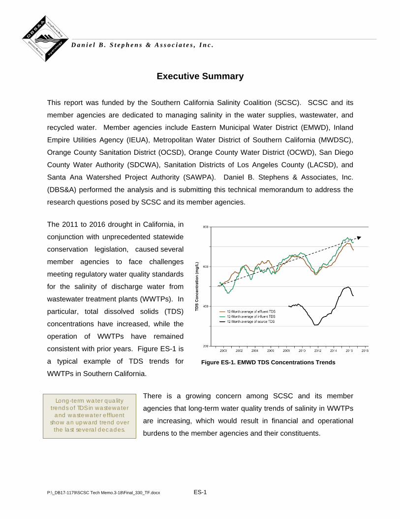
The 2011 to 2016 drought in California, in
conjunction with unprecedented statewide
conservation legislation, caused several
member agencies to face challenges
meeting regulatory water quality standards
for the salinity of discharge water from
wastewater treatment plants (WWTPs). In
particular, total dissolved solids (TDS)
concentrations have increased, while the
operation of WWTPs have remained
consistent with prior years. Figure ES-1 is
a typical example of TDS trends for
WWTPs in Southern California.
There is a growing concern among SCSC and its member
agencies that long-term water quality trends of salinity in WWTPs
are increasing, which would result in financial and operational
burdens to the member agencies and their constituents.
Figure ES-1. EMWD TDS Concentrations Trends
Long-term water quality trends of TDS in wastewater
and wastewater effluent show an upward trend over
the last several decades.
P:\_DB17-1179\SCSC Tech Memo.3-18\Final_330_TF.docx ES-2
D a n i e l B . S t e p h e n s & A s s o c i a t e s , I n c .
This analysis considered a series of research questions, the purpose of which is to provide a
quantitative understanding of the relationships among variables such as salt concentrations in
municipal influent and treated effluent, drought, self-regenerating water softeners (SRWS), and
the mandated implementation of water conservation practices that reduce per capita water use.
The findings from this research will be of particular value to water supply and wastewater
treatment and recycling agencies as they consider how changes in water quality and quantity
may impact their ability to provide reliable, high-quality drinking water while complying with
waste discharge requirements.
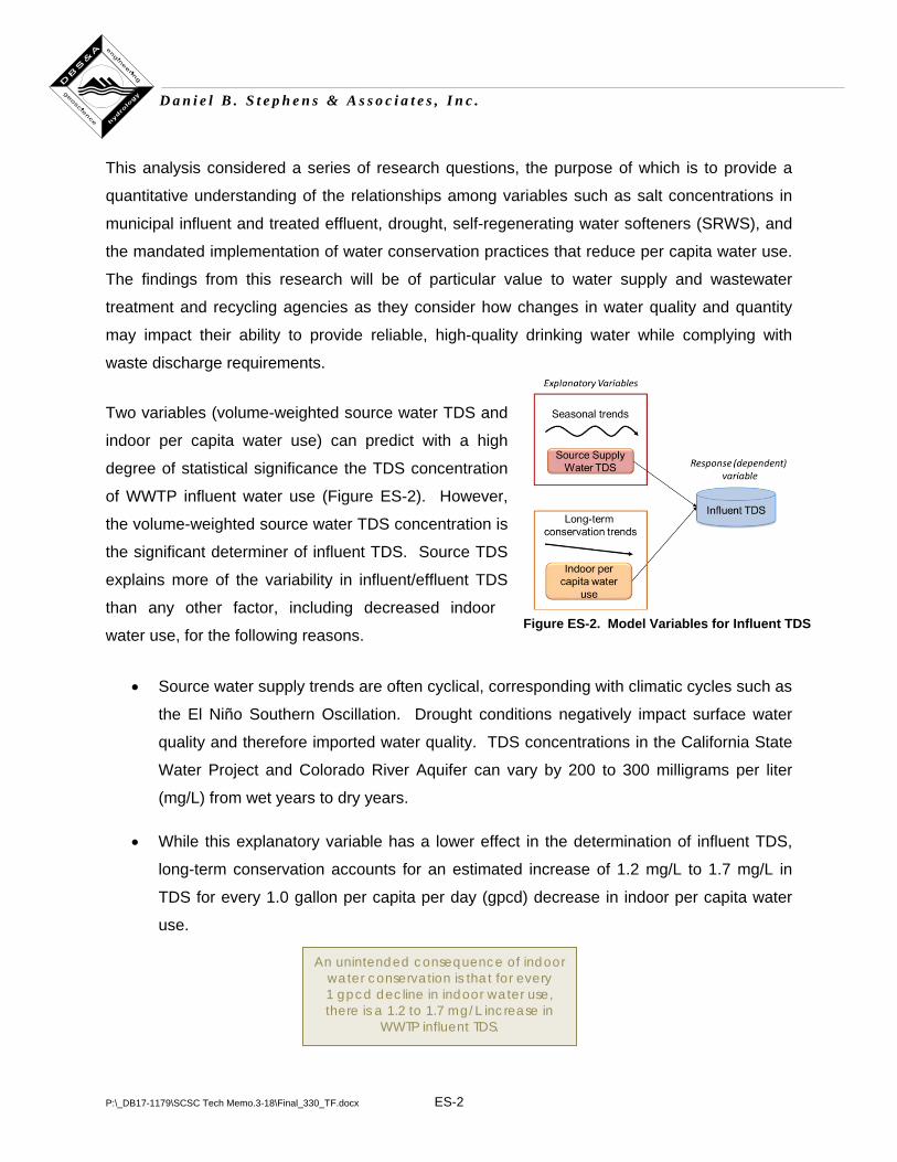
Two variables (volume-weighted source water TDS and
indoor per capita water use) can predict with a high
degree of statistical significance the TDS concentration
of WWTP influent water use (Figure ES-2). However,
the volume-weighted source water TDS concentration is
the significant determiner of influent TDS. Source TDS
explains more of the variability in influent/effluent TDS
than any other factor, including decreased indoor
water use, for the following reasons.
• Source water supply trends are often cyclical, corresponding with climatic cycles such as
the El Niño Southern Oscillation. Drought conditions negatively impact surface water
quality and therefore imported water quality. TDS concentrations in the California State
Water Project and Colorado River Aquifer can vary by 200 to 300 milligrams per liter
(mg/L) from wet years to dry years.
• While this explanatory variable has a lower effect in the determination of influent TDS,
long-term conservation accounts for an estimated increase of 1.2 mg/L to 1.7 mg/L in
TDS for every 1.0 gallon per capita per day (gpcd) decrease in indoor per capita water
use.
Figure ES-2. Model Variables for Influent TDS
An unintended consequence of indoor water conservation is that for every 1 gpcd decline in indoor water use, there is a 1.2 to 1.7 mg/L increase in
WWTP influent TDS.
P:\_DB17-1179\SCSC Tech Memo.3-18\Final_330_TF.docx ES-3
D a n i e l B . S t e p h e n s & A s s o c i a t e s , I n c .
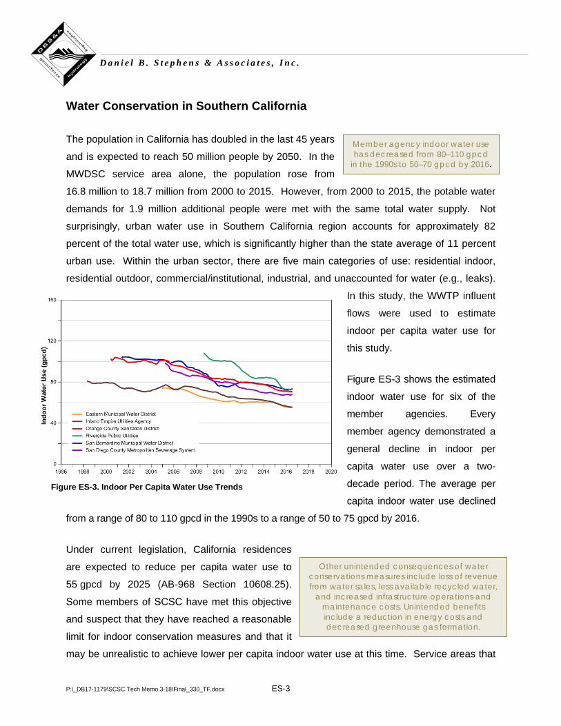
Member agency indoor water use has decreased from 80–110 gpcd
in the 1990s to 50–70 gpcd by 2016.
Water Conservation in Southern California
The population in California has doubled in the last 45 years
and is expected to reach 50 million people by 2050. In the
MWDSC service area alone, the population rose from
16.8 million to 18.7 million from 2000 to 2015. However, from 2000 to 2015, the potable water
demands for 1.9 million additional people were met with the same total water supply. Not
surprisingly, urban water use in Southern California region accounts for approximately 82
percent of the total water use, which is significantly higher than the state average of 11 percent
urban use. Within the urban sector, there are five main categories of use: residential indoor,
residential outdoor, commercial/institutional, industrial, and unaccounted for water (e.g., leaks).
In this study, the WWTP influent
flows were used to estimate
indoor per capita water use for
this study.
Figure ES-3 shows the estimated
indoor water use for six of the
member agencies. Every
member agency demonstrated a
general decline in indoor per
capita water use over a two-
decade period. The average per
capita indoor water use declined
from a range of 80 to 110 gpcd in the 1990s to a range of 50 to 75 gpcd by 2016.
Under current legislation, California residences
are expected to reduce per capita water use to
55 gpcd by 2025 (AB-968 Section 10608.25).
Some members of SCSC have met this objective
and suspect that they have reached a reasonable
limit for indoor conservation measures and that it
may be unrealistic to achieve lower per capita indoor water use at this time. Service areas that
Other unintended consequences of water conservations measures include loss of revenue from water sales, less available recycled water,
and increased infrastructure operations and maintenance costs. Unintended benefits include a reduction in energy costs and decreased greenhouse gas formation.
Figure ES-3. Indoor Per Capita Water Use Trends
P:\_DB17-1179\SCSC Tech Memo.3-18\Final_330_TF.docx ES-4
D a n i e l B . S t e p h e n s & A s s o c i a t e s , I n c .
have not reached this 55 gpcd goal will likely continue to see a downward trend in per capita
water use. The implication for continued decrease in indoor per capita water use is that WWTP
influent TDS will increase by an estimated 1.2 to 1.7 mg/L for every 1.0 gpcd decrease in indoor
water use.
Climate Cycles and Source Supply Water
There is a strong inverse correlation between surface
water quality and the long-term meteorological
cycles, including drought cycles. One way to
evaluate drought is through the Palmer Drought
Severity Index (PDSI), established by the National
Oceanic and Atmosphere Administration. While this study focuses on WWTPs in Southern
California, a drought in Northern California can change TDS in source water supply in Southern
California. Likewise, drought conditions in the Rocky Mountains affect TDS in the Colorado
River. This analysis uses the drought index for the entire state of California as a generalization
of drought conditions. Local drought indices will vary across hydrologic regions.
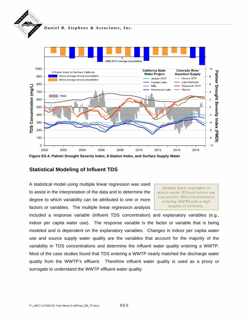
Another way to analyze long-term meteorological cycles is through the 8-Station Index. This
method compares the annual precipitation of 8 key stations in Northern California to the annual
average precipitation measured at these stations from 1966 to 2015. The 8-station index is
used to help manage state water supplies, including how much low-salinity State Water Project
(SWP) water is available to Southern California. Figure ES-4 compares the PMDI and 8-Station
Index to surface supply water quality data for major reservoirs and treatment facilities operated
by MWDSC. Time-series TDS concentrations are shown for Skinner Lake, Lake Mathews,
Deimer WTP, and Weymouth WTP as part of the Colorado River Aqueduct, and for Mills,
Silverwood Lake, Castaic Lake, and Jensen WTP as part of the SWP. Aside from Lake
Mathews, which has a more gradual trend, all reservoirs show similar increases in TDS during
periods of drought and decreases in TDS during wet years.
There is a strong inverse correlation between drought and imported water TDS concentrations - for both SWP water and
CRA water. TDS concentration can vary by 300 mg/L from wet years to dry years for
CRA water and by 200 mg/L for SWP water.
P:\_DB17-1179\SCSC Tech Memo.3-18\Final_330_TF.docx ES-5
D a n i e l B . S t e p h e n s & A s s o c i a t e s , I n c .
Figure ES-4. Palmer Drought Severity Index, 8-Station Index, and Surface Supply Water
Statistical Modeling of Influent TDS
A statistical model using multiple linear regression was used
to assist in the interpretation of the data and to determine the
degree to which variability can be attributed to one or more
factors or variables. The multiple linear regression analysis
included a response variable (influent TDS concentration) and explanatory variables (e.g.,
indoor per capita water use). The response variable is the factor or variable that is being
modeled and is dependent on the explanatory variables. Changes in indoor per capita water
use and source supply water quality are the variables that account for the majority of the
variability in TDS concentrations and determine the influent water quality entering a WWTP.
Most of the case studies found that TDS entering a WWTP nearly matched the discharge water
quality from the WWTP’s effluent. Therefore influent water quality is used as a proxy or
surrogate to understand the WWTP effluent water quality.
Multiple linear regression of source water TDS and indoor use can predict TDS concentrations
entering WWTPs with a high degree of certainty.
P:\_DB17-1179\SCSC Tech Memo.3-18\Final_330_TF.docx ES-6
D a n i e l B . S t e p h e n s & A s s o c i a t e s , I n c .
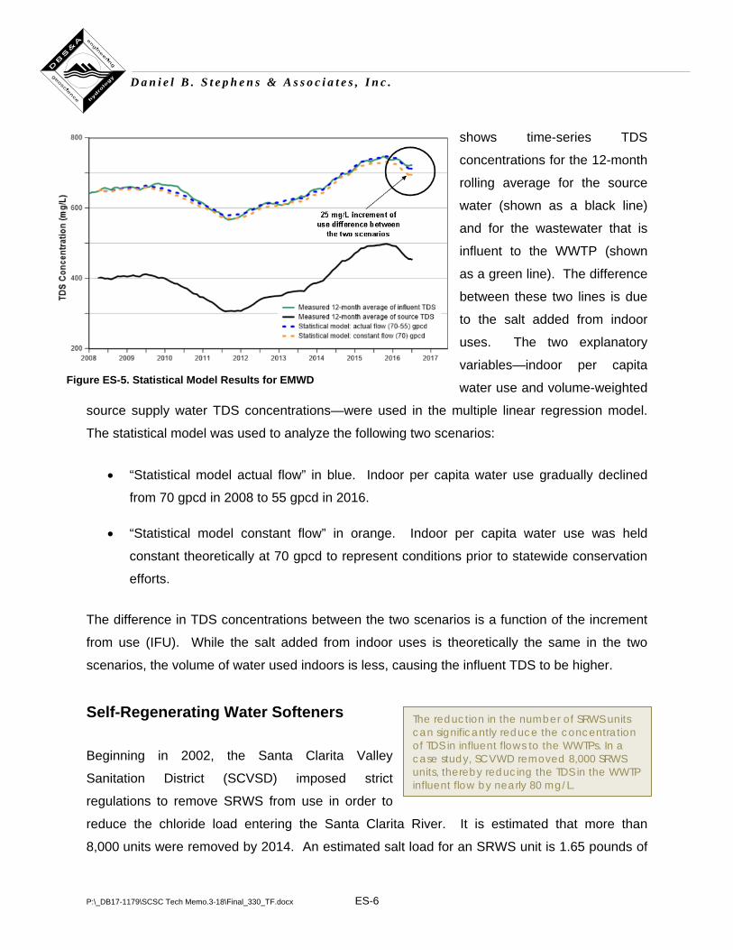
shows time-series TDS
concentrations for the 12-month
rolling average for the source
water (shown as a black line)
and for the wastewater that is
influent to the WWTP (shown
as a green line). The difference
between these two lines is due
to the salt added from indoor
uses. The two explanatory
variables—indoor per capita
water use and volume-weighted
source supply water TDS concentrations—were used in the multiple linear regression model.
The statistical model was used to analyze the following two scenarios:
• “Statistical model actual flow” in blue. Indoor per capita water use gradually declined
from 70 gpcd in 2008 to 55 gpcd in 2016.
• “Statistical model constant flow” in orange. Indoor per capita water use was held
constant theoretically at 70 gpcd to represent conditions prior to statewide conservation
efforts.
The difference in TDS concentrations between the two scenarios is a function of the increment
from use (IFU). While the salt added from indoor uses is theoretically the same in the two
scenarios, the volume of water used indoors is less, causing the influent TDS to be higher.
Self-Regenerating Water Softeners
Beginning in 2002, the Santa Clarita Valley
Sanitation District (SCVSD) imposed strict
regulations to remove SRWS from use in order to
reduce the chloride load entering the Santa Clarita River. It is estimated that more than
8,000 units were removed by 2014. An estimated salt load for an SRWS unit is 1.65 pounds of
The reduction in the number of SRWS units can significantly reduce the concentration of TDS in influent flows to the WWTPs. In a case study, SCVWD removed 8,000 SRWS units, thereby reducing the TDS in the WWTP influent flow by nearly 80 mg/L.
Figure ES-5. Statistical Model Results for EMWD
P:\_DB17-1179\SCSC Tech Memo.3-18\Final_330_TF.docx ES-7
D a n i e l B . S t e p h e n s & A s s o c i a t e s , I n c .
salt per day per unit. The average flow for the SCVSD treatment facilities between 2002 and
2014 was 20 million gallon per day (mgd). Using the following equation (with the appropriate
unit conversions), it is estimated that nearly 80 mg/L of TDS was removed from the system by
removing SWRS units:
TDS removed= Number of SWS units ×1.65 pounds of salt per day per unitFlow into the WWTP
Of the 26 WWTPs in the study that provided influent TDS data, only 4 WWTPs demonstrated a
downward trend in TDS; the 2 WWTPs in the SCVSD are among those. The remaining
WWTPs either demonstrated an upward trend or a flat trend. The downward trend in TDS
concentrations over the study period for the WWTPs in the SCVSD service area are likely a
result of the systematic removal of SRWS units.
P:\_DB17-1179\SCSC Tech Memo.3-18\Final_330_TF.docx 1
D a n i e l B . S t e p h e n s & A s s o c i a t e s , I n c .
1. Background and Understanding
This report was funded by the Southern California Salinity Coalition (SCSC). The objective of
SCSC, which consists of water and wastewater agencies in southern California, is “to address
the critical need to remove salt from water supplies and to preserve water resources in
California” (SCSC, 2017). SCSC and its member agencies are dedicated to managing salinity
in the water supplies, wastewater, and recycled water. Member agencies include Eastern
Municipal Water District (EMWD), Inland Empire Utilities Agency (IEUA), Metropolitan Water
District of Southern California (MWDSC), Orange County Sanitation District (OCSD), Orange
County Water District (OCWD), San Diego County Water Authority (SDCWA), Sanitation
Districts of Los Angeles County (LACSD), and Santa Ana Watershed Project Authority
(SAWPA). Daniel B. Stephens & Associates, Inc. (DBS&A) performed the analysis and is
submitting this technical memorandum to address the research questions posed by SCSC and
its member agencies.
The water supply for Southern California originates from a variety of sources, both imported and
local. In general, water is imported into the Southern California region from the Sacramento/
San Joaquin Delta through the State Water Project (SWP), from the Colorado River through the
Colorado River Aqueduct (CRA), and from the Owens Valley/Mono Basin areas through the Los
Angeles Aqueduct. Much of the imported water is then distributed to the SCSC member
agencies through MWDSC. These imported sources supplement local water development
projects (e.g., local surface water, groundwater [including treated and desalinated groundwater],
recycled water, stormwater recharge, and desalinated seawater). Local agencies also
implement conjunctive use programs (i.e., storage and recovery of imported water in
groundwater basins and local surface reservoirs) to increase the reliability of local supplies
during dry periods and in anticipation of interruptions in imported supply from catastrophic
events. Local conservation efforts also support water supply needs by reducing the overall
water demand in the region.
Water agencies routinely use a mix of imported and local water sources to meet their water
supply needs at an acceptable water quality. The average water quality of these various water
sources is known and can be managed to create an appropriate blend to control the level of
P:\_DB17-1179\SCSC Tech Memo.3-18\Final_330_TF.docx 2
D a n i e l B . S t e p h e n s & A s s o c i a t e s , I n c .
salinity in the delivered water and subsequent wastewater. However, changes in the blend of
available sources of water, as well as fluctuations in their salinity, can alter typical expected
salinity levels. For example, the 2013 California Water Plan (DWR, 2013) notes that all three
key imported water sources for the southern California region will become less reliable sources
of water—in terms of both quantity and quality—due to anticipated climate change impacts and
requirements to address environmental concerns.
1.1 Indoor Water Use
Total water use can be separated into three main sectors of water use: urban, agricultural, and
environmental—which includes the preservation of aquatic habitat and/or protection of
endangered species. In 2010, the use of water in California was about 50 percent
environmental, 40 percent agricultural, and 10 percent urban (Mount and Hanak, 2016).
According to California Department of Water Resources (DWR), between 2001 and 2010, urban
water use accounted for 9,084 acre-feet per year (ac-ft/yr), or approximately 11 percent of the
total water use for the entire state of California. All of the member agencies for this study are
within the South Coast DWR hydrologic region, which extends along the coast from Ventura to
San Diego and eastward to San Bernardino. Urban water use in the South Coast hydrologic
region accounts for approximately 82 percent of the total water use. For comparison, Table 1
shows the average water use by main sector for each of the DWR hydrologic regions for the
period 2001 to 2010.
Within the urban sector, there are five main categories: residential indoor, residential outdoor,
commercial/institutional, industrial, and unaccounted for water (i.e., leaks). Figure 1 is a
simplified flow diagram that represents the water supplies that reach Southern California
wastewater treatment plants (WWTPs). The gross water supply (source water) is split into two
components: (1) water that will ultimately reach the WWTP and (2) water that reenters the
environment through agriculture or irrigation, or is sent to brine lines. The component that
reaches the WWTP consists of indoor residential, commercial, and industrial uses and
represents the flow and quality of the WWTP influent.

P:\_DB17-1179\SCSC Tech Memo.3-18\Final_330_TF.docx 3
D a n i e l B . S t e p h e n s & A s s o c i a t e s , I n c .
Table 1. Average Water Use by Main Sectors by DWR Hydrologic Region, 2001–2010
Average Water Use (ac-ft/yr) DWR Hydrologic Region Environmental Agricultural Urban
North Coast 18,865 833 155 San Francisco Bay 24 123 1,192 Central Coast 101 1,066 305 South Coast 127 769 4,162 Sacramento River 13,690 8,664 904 San Joaquin River 3,067 7,415 674 Tulare Lake 1,560 10,832 744 North Lahontan 340 492 43 South Lahontan 81 382 278 Colorado River 30 4,001 627
Total 37,885 34,577 9,084
Source: DWR, 2013 ac-ft/yr = Acre-feet per year
Figure 1. Flow Diagram of Water Supply and Water Uses for WWTPs
Water delivered for residential, commercial, and industrial sectors is used for both indoor and
outdoor applications; in this study, indoor uses are analyzed because water used indoors
becomes influent water to WWTPs (with the exception of leaks). DeOreo et al. (2017) found in
their study that the split is about 53 percent outdoors and 47 percent indoors for a sample of
CRA
SWP
Wells
Gross Water Supply Residential,
Commercial, Institutional
Landscaping
Indoor Uses
WWTP
WWTP Influent
WWTP Effluent
Recycled Agricultural, Industrial
P:\_DB17-1179\SCSC Tech Memo.3-18\Final_330_TF.docx 4
D a n i e l B . S t e p h e n s & A s s o c i a t e s , I n c .
their study that the split is about 53 percent outdoors and 47 percent indoors for a sample of
735 single-family homes from 10 water agencies in California. In the 2017 study, the total
annual water use was 362 gallons per household per day (gphd). Based on an average
occupancy rate of 2.94 persons per home, the per capita total water use was 123 gallons per
capita per day (gpcd); at 47 percent, the indoor use was 57.9 gpcd.
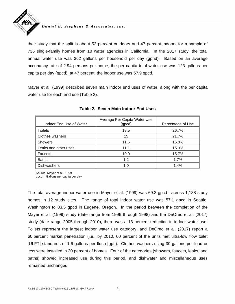
Mayer et al. (1999) described seven main indoor end uses of water, along with the per capita
water use for each end use (Table 2).
Table 2. Seven Main Indoor End Uses
Indoor End Use of Water Average Per Capita Water Use
(gpcd) Percentage of Use
Toilets 18.5 26.7% Clothes washers 15 21.7% Showers 11.6 16.8% Leaks and other uses 11.1 15.9% Faucets 10.9 15.7% Baths 1.2 1.7% Dishwashers 1.0 1.4%
Source: Mayer et al., 1999 gpcd = Gallons per capita per day
The total average indoor water use in Mayer et al. (1999) was 69.3 gpcd—across 1,188 study
homes in 12 study sites. The range of total indoor water use was 57.1 gpcd in Seattle,
Washington to 83.5 gpcd in Eugene, Oregon. In the period between the completion of the
Mayer et al. (1999) study (date range from 1996 through 1998) and the DeOreo et al. (2017)
study (date range 2005 through 2010), there was a 13 percent reduction in indoor water use.
Toilets represent the largest indoor water use category, and DeOreo et al. (2017) report a
60 percent market penetration (i.e., by 2010, 60 percent of the units met ultra-low flow toilet
[ULFT] standards of 1.6 gallons per flush [gpf]). Clothes washers using 30 gallons per load or
less were installed in 30 percent of homes. Four of the categories (showers, faucets, leaks, and
baths) showed increased use during this period, and dishwater and miscellaneous uses
remained unchanged.
P:\_DB17-1179\SCSC Tech Memo.3-18\Final_330_TF.docx 5
D a n i e l B . S t e p h e n s & A s s o c i a t e s , I n c .
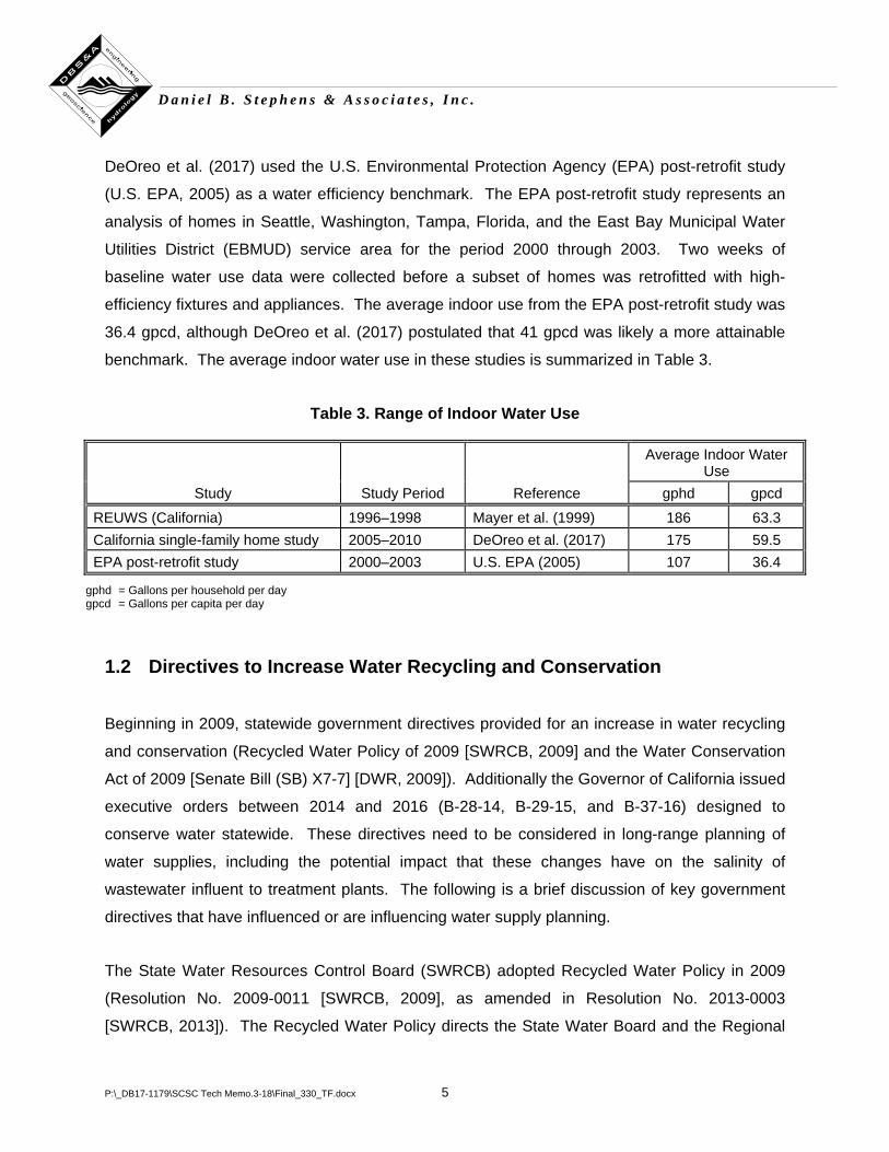
DeOreo et al. (2017) used the U.S. Environmental Protection Agency (EPA) post-retrofit study
(U.S. EPA, 2005) as a water efficiency benchmark. The EPA post-retrofit study represents an
analysis of homes in Seattle, Washington, Tampa, Florida, and the East Bay Municipal Water
Utilities District (EBMUD) service area for the period 2000 through 2003. Two weeks of
baseline water use data were collected before a subset of homes was retrofitted with high-
efficiency fixtures and appliances. The average indoor use from the EPA post-retrofit study was
36.4 gpcd, although DeOreo et al. (2017) postulated that 41 gpcd was likely a more attainable
benchmark. The average indoor water use in these studies is summarized in Table 3.
Table 3. Range of Indoor Water Use
Average Indoor Water
Use Study Study Period Reference gphd gpcd
REUWS (California) 1996–1998 Mayer et al. (1999) 186 63.3 California single-family home study 2005–2010 DeOreo et al. (2017) 175 59.5 EPA post-retrofit study 2000–2003 U.S. EPA (2005) 107 36.4
gphd = Gallons per household per day gpcd = Gallons per capita per day
1.2 Directives to Increase Water Recycling and Conservation
Beginning in 2009, statewide government directives provided for an increase in water recycling
and conservation (Recycled Water Policy of 2009 [SWRCB, 2009] and the Water Conservation
Act of 2009 [Senate Bill (SB) X7-7] [DWR, 2009]). Additionally the Governor of California issued
executive orders between 2014 and 2016 (B-28-14, B-29-15, and B-37-16) designed to
conserve water statewide. These directives need to be considered in long-range planning of
water supplies, including the potential impact that these changes have on the salinity of
wastewater influent to treatment plants. The following is a brief discussion of key government
directives that have influenced or are influencing water supply planning.
The State Water Resources Control Board (SWRCB) adopted Recycled Water Policy in 2009
(Resolution No. 2009-0011 [SWRCB, 2009], as amended in Resolution No. 2013-0003
[SWRCB, 2013]). The Recycled Water Policy directs the State Water Board and the Regional
P:\_DB17-1179\SCSC Tech Memo.3-18\Final_330_TF.docx 6
D a n i e l B . S t e p h e n s & A s s o c i a t e s , I n c .
Water Quality Control Boards (Regional Boards) to “exercise the authority granted to them by
the state legislature to the fullest extent possible to encourage the use of recycled water,
consistent with state and federal water quality laws” so that water suppliers can become
independent of reliance on “the vagaries of annual precipitation and move towards sustainable
management of surface water and groundwater, together with enhanced water conservation,
water reuse and the use of stormwater.” The Recycled Water Policy also recognizes that
encouraging increased recycled water use requires increased attention to potential
management of salt and nutrient impacts that may result. Accordingly, the Recycled Water
Policy requires the Regional Boards to develop and implement salt and nutrient management
plans to ensure attainment of water quality objectives and protection of beneficial uses.
Subsequent to the adoption of the Recycled Water Policy, the California Legislature approved
the Water Conservation Act of 2009 (DWR, 2009), which established a number of water
conservation requirements, including the goal to obtain a 20 percent reduction in urban per
capita water use, consistent with the goals of the Recycled Water Policy (SWRCB, 2009). This
20 percent reduction goal is to be achieved by December 31, 2020.
The Governor issued a number of executive orders to address the 2011 to 2016 drought, which
has resulted in significant overdraft of groundwater basins throughout the state. At the
drought’s peak, over 90 percent of California was classified as being in an “exceptional” drought
period, which is the worst drought classification. Given the significance of this drought,
Governor Edmund G. Brown Jr. declared a state of emergency on January 17, 2014, “directed
state officials to take all necessary actions to prepare for these drought conditions,” and called
for Californians to reduce water use by 20 percent (CED, 2014a). Three months later, Governor
Brown “issued an executive order to strengthen the state’s ability to manage water and habitat
effectively in drought conditions and called on all Californians to redouble their efforts to
conserve water” (CED, 2014b). On April 1, 2015, the Governor directed the State Water Board
to implement mandatory water reductions. The targeted reduction is 25 percent less potable
urban water use statewide when compared to the amount of water used in 2013 (CED, 2015).
May 9, 2016, Governor Brown issued executive order B-37-16 (CED, 2016), commonly referred
to as “Making Water Conservation a California Way of Life,” to bolster California’s climate and
P:\_DB17-1179\SCSC Tech Memo.3-18\Final_330_TF.docx 7
D a n i e l B . S t e p h e n s & A s s o c i a t e s , I n c .
drought resilience. This executive order was designed to incorporate the lessons learned from
the temporary statewide emergency water restrictions and apply them to establish a long-term
water conservation framework. Legislation was passed on February 16, 2017 to update the
Water Code (AB-968 Section 10608.25) (CED, 2017a), wherein urban retail water suppliers
shall develop a water efficiency target for 2025 that meets either 75 percent of urban retail water
suppliers base daily per capita water use calculated in Section 10608.2 or establish a retail-level
efficiency target that among several factors is based upon population multiplied by 55 gpcd.
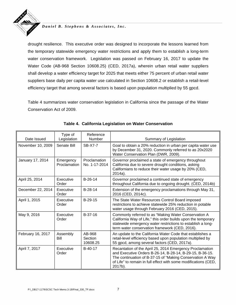
Table 4 summarizes water conservation legislation in California since the passage of the Water
Conservation Act of 2009.
Table 4. California Legislation on Water Conservation
Date Issued Type of
Legislation Reference Number Summary of Legislation
November 10, 2009 Senate Bill SB-X7-7 Goal to obtain a 20% reduction in urban per capita water use by December 31, 2020. Commonly referred to as 20x2020 Water Conservation Plan (DWR, 2009).
January 17, 2014 Emergency Proclamation
Proclamation No. 1-17-2014
Governor proclaimed a state of emergency throughout California due to severe drought conditions, asking Californians to reduce their water usage by 20% (CED, 2014a).
April 25, 2014 Executive Order
B-26-14 Governor proclaimed a continued state of emergency throughout California due to ongoing drought. (CED, 2014b)
December 22, 2014 Executive Order
B-28-14 Extension of the emergency proclamations through May 31, 2016 (CED, 2014c).
April 1, 2015 Executive Order
B-29-15 The State Water Resources Control Board imposed restrictions to achieve statewide 25% reduction in potable water usage through February 2016 (CED, 2015).
May 9, 2016 Executive Order
B-37-16 Commonly referred to as “Making Water Conservation A California Way of Life,” this order builds upon the temporary statewide emergency water restrictions to establish a long-term water conservation framework (CED, 2016).
February 16, 2017 Assembly Bill
AB-968 Section 10608.25
An update to the California Water Code that establishes a retail-level efficiency based upon population multiplied by 55 gpcd, among several factors (CED, 2017a).
April 7, 2017 Executive Order
B-40-17 Recantation of the April 25, 2014 Emergency Proclamation and Executive Orders B-26-14, B-28-14, B-29-15, B-36-15. The continuation of B-37-15 of “Making Conservation A Way of Life” to remain in full effect with some modifications (CED, 2017b).
P:\_DB17-1179\SCSC Tech Memo.3-18\Final_330_TF.docx 8
D a n i e l B . S t e p h e n s & A s s o c i a t e s , I n c .
1.3 Impacts of Drought Water Conservation on Wastewater Conveyance
Systems and WWTP Operations
The impact of indoor water conservation on wastewater flows—and, by extension, WWTP
operations and discharge water quality—has been discussed for decades. Prompted by the
severe drought in California in 1976 to 1977, the EPA conducted a study to quantify the effects
of water conservation on the reduction of wastewater influent flows to WWTPs (U.S. EPA,
1980). The drought-induced reductions in flow were used as a surrogate for projecting the
impact of conservation measures.
The study noted that “during the last 10 years, urban water conservation has attracted much
attention and has widely become to be considered as an essential part of effectively managing
our water resources” (U.S. EPA, 1980). Some of the indoor water conservation measures
employed in the mid- to late-1970s include “. . . installing low-flow faucet aerators, low-flow
shower heads or flow restrictors, and ‘water dams’ or plastic bottles in toilet tanks to reduce the
amount of water used for flushing” (U.S. EPA, 1980).
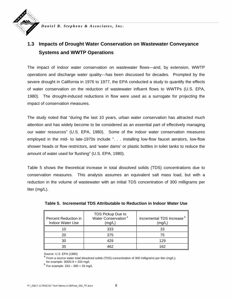
Table 5 shows the theoretical increase in total dissolved solids (TDS) concentrations due to
conservation measures. This analysis assumes an equivalent salt mass load, but with a
reduction in the volume of wastewater with an initial TDS concentration of 300 milligrams per
liter (mg/L).
Table 5. Incremental TDS Attributable to Reduction in Indoor Water Use
Percent Reduction in Indoor Water Use
TDS Pickup Due to Water Conservation a
(mg/L) Incremental TDS Increase b
(mg/L)
10 333 33 20 375 75 30 429 129 35 462 162
Source: U.S. EPA (1980) a From a source water total dissolved solids (TDS) concentration of 300 milligrams per liter (mg/L);
for example: 300/0.9 = 333 mg/L b For example: 333 – 300 = 33 mg/L
P:\_DB17-1179\SCSC Tech Memo.3-18\Final_330_TF.docx 9
D a n i e l B . S t e p h e n s & A s s o c i a t e s , I n c .
The California Urban Water Agencies (CUWA) published a white paper in November 2017 that
summarizes the impacts of declining flows on water distribution systems, wastewater
conveyance systems, wastewater treatment plant operations, and recycled water projects. The
study was based on a literature review, a high-level survey, and focused interviews with
individual water agencies in California. CUWA (2017) notes that, the “effluent from WWTPs is
held to standards mandated by their individual National Pollutant Discharge Elimination System
(NPDES) permits, including effluent quality limits for constituents like ammonia. . . Increasing
influent concentrations can impact effluent quality, straining a plant’s ability to meet its discharge
permit requirements. To avoid exceeding permit limits, utilities may have to consider
implementing costly WWTP upgrades.” In the survey, 40 percent of WWTPs were impacted by
increased concentrations of TDS, ammonia, or other constituents, resulting in challenges with
effluent quality limits.
1.4 Salt Mass Loading
The American Water Works Association Research Foundation (AWWARF) and the WateReuse
Foundation jointly funded the study Characterizing and Managing Salinity Loadings in
Reclaimed Water Systems (Thompson et al., 2006). This study was a comprehensive review of
the “problem of salinity in reclaimed water on a national level” (Thompson et al., 2006). Salinity
increases in reclaimed water can limit its use on crops, landscape, golf courses, and industrial
uses. According to Thompson et al. (2006), “When water passes through municipal systems, it
gains salts (‘salt pickup’), typically adding 200–400 mg/L TDS.” This report uses the term salt
mass load (SML) to define the mass of salt loaded to the system over a period of time (e.g., one
day), whereas Thompson et al. (2006) use the term “TDS contribution.” Likewise, this report
uses the term increment from use (IFU) to express the TDS concentration (mass/volume)
increases, while Thompson et al. (2006) refer to “TDS gain.”
In residential use, the average person excretes between about 70 grams (Thompson et al.,
2006) and 72.8 grams (Nall and Sedak, 2013) of salt each day. About 45 grams per capita per
day are excreted in urine and about half of this is in the form of urea, a soluble organic
compound that degrades over time (Aparicio et al., 2017). Because urea is not measured as a
component of TDS, the mass of measurable salt excreted by the average individual is between

P:\_DB17-1179\SCSC Tech Memo.3-18\Final_330_TF.docx 10
D a n i e l B . S t e p h e n s & A s s o c i a t e s , I n c .
about 47.5 and 50.3 grams per capita per day. Gray water (showers, baths, clothes washing
machines, and wastewater that does not contain fecal contamination) adds about 20 to
30 grams per capita per day, including about 10 grams per capita per day from detergents and
2 grams per capita per day from in-sink food disposals. Hence, the SML from indoor use is
approximately 0.15 to 0.18 pound per capita per day. However, WWTPs also receive water
from commercial and industrial sources, which may increase or decrease the SML values of
wastewater entering a WWTPs and therefore affect the estimated per capita salt load per day.
Tran et al. (2017) note that “. . . a simple water balance thought experiment illustrates that
drought, and the conservation strategies that are often enacted in response to it, both likely limit
the role reuse may play in improving local water supply reliability.” This study analyzed influent
flow and water quality data for IEUA’s Regional Plant 1 (RP1) from 2011 through 2015. Tran et
al. (2017) note that “as a particular drought progresses and agencies enact water conservation
measures to cope with drought, influent flows likely decrease while influent pollution
concentrations increase, particularly salinity, which adversely affects wastewater treatment plant
(WWTP) costs and effluent quality and flow. Consequently, downstream uses of this effluent,
whether to maintain streamflow and quality, groundwater recharge, or irrigation may be
impacted,” leading to the conclusion that “indoor conservation can result in the generation of a
more concentrated wastewater stream, with elevated concentrations of total dissolved solids
(TDS), nitrogen species, and carbon.”
1.5 Impact of Self-Regenerating Water Softeners
Water hardness is defined by the amount of dissolved calcium and magnesium in the water.
Hard water can cause staining and scaling on dishes, appliances, plumbing fixtures, and
adversely affects taste and texture of drinking water (USGS, 2016a). The scaling can reduce
the useful lifespan of equipment (USGS, 2016b), clog pipes, and increase the cost of heating
water. For many years, water softeners have been installed and operated in residential and
commercial properties with water supplies containing higher levels of hardness, as they provide
a service by reducing scale in customer appliances and fixtures.
P:\_DB17-1179\SCSC Tech Memo.3-18\Final_330_TF.docx 11
D a n i e l B . S t e p h e n s & A s s o c i a t e s , I n c .
There are two types of water softeners in residential use: self-regenerating water softeners
(SRWS), also known as automatic water softeners, and exchange tank systems. SRWS use
ion exchange technology, wherein the unit contains negatively charged resin with positively
charged sodium ions sorbed to the surface. The calcium and magnesium ions are exchanged
with the sodium ions because they have a higher charge density due to a higher valence state
(+2 versus +1). When most of the sodium ions have been removed from the resin, the system
is regenerated by adding a solution of sodium chloride or potassium chloride from an on-site
brine tank. The high concentration of sodium or potassium ions swamp the calcium and
magnesium ions sorbed to the resin surface. After regeneration, the system’s brine waste,
containing calcium, magnesium, and chloride, is discharged to the municipal sewer system. In
exchange tank systems, a vendor replaces an exhausted tank with a newly regenerated tank;
the regeneration takes place at an off-site location where the regenerated brine can be
managed appropriately, minimizing impacts to publically owned treatment works (POTWs).
As discussed previously, conventional WWTPs do not remove TDS or the major ions that
contribute to TDS, such as calcium, magnesium, or chloride; therefore, concentrations of these
constituents in wastewater influent are higher in sewer service areas where SRWS are or used
to be allowed than they would be absent the use of SRWS. Effective January 1, 2003, SB-1006
allows prospective water softener prohibitions if a WWTP is in non-compliance with permits and
completes extensive studies. With the passage of AB-1366 in 2009, local agencies or cities that
own or operate a community sewer system or water recycling facility have the authority to
regulate SRWS.
1.6 Study to Evaluate Long-Term Trends and Variations in the Average TDS Concentration in Wastewater and Recycled Water
Given the complexity of factors that can influence the salinity of source waters and wastewater
influent and effluent, the SCSC commissioned this study to analyze the relationship of the
effects of drought, water conservation practices, and the quality of recycled water.
Conservation measures may have unintended consequences that are beneficial, such as the
electricity savings and greenhouse gas emissions reductions associated with reduced operation
of urban water infrastructure (Spang et al., 2018), as well as consequences that are
P:\_DB17-1179\SCSC Tech Memo.3-18\Final_330_TF.docx 12
D a n i e l B . S t e p h e n s & A s s o c i a t e s , I n c .
undesirable, including for recycled water reuse by impacting water quality downstream uses of
recycled water: irrigation, groundwater recharge, industrial uses, or releases to aquatic habitats.
This analysis considered a series of research questions, the purpose of which is to provide a
quantitative understanding of the relationships among variables such as salt concentrations in
municipal influent and treated effluent, impact of water softener devices on salt concentrations
in influent, and implementation of conservation practices that reduce per capita water use. The
potential link between these various factors is important in predicting how salinity relative to
water use may continue to change in the future.
The findings from this research will be of particular value to water supply and wastewater
treatment and recycling agencies as they consider how changes in the future may impact their
ability to provide reliable, high-quality drinking water while complying with waste discharge
requirements. In addition, the findings can be evaluated in the context of the following factors
that have the potential to further influence the availability of water (and associated quality) from
various sources in the future:
• Climate change: Climate change currently has the potential to significantly alter the
hydrology of the Sierra Nevada Mountains (the main source of water that flows through
the Delta and SWP) and the Rocky Mountains (the main source of water for the
Colorado River System). State Water Board Resolution No. 2017-0012, Comprehensive
Response to Climate Change, states that “Changes in hydrology include declining
snowpack and more frequent and longer droughts, more frequent and more severe
flooding, changes in the timing and volume of peak runoff, and consequent impacts on
water quality and water availability.”
• Bay Delta management: Environmental regulations concerning endangered fish species
or other requirements could significantly restrict Delta water exports in the future. The
Bay Delta Conservation Plan (BDCP) (U.S. EPA, 2018) “was a habitat conservation plan
proposed by the California Department of Water Resources, U.S. Fish & Wildlife
Service, National Marine Fisheries Service, and Bureau of Reclamation, under the
Endangered Species Act, to address the most critical water issues facing California by
constructing new water delivery infrastructure and restoring aquatic habitat. In 2015, the

P:\_DB17-1179\SCSC Tech Memo.3-18\Final_330_TF.docx 13
D a n i e l B . S t e p h e n s & A s s o c i a t e s , I n c .
Bay Delta Conservation Plan was recast as California WaterFix, with a focus on the
construction and operation of proposed new water export intakes on the Sacramento
River to divert water into a proposed 40 mile twin tunnel conveyance facility” (U.S. EPA,
2018).
• Colorado River System: Drought and increasing water demands in the Colorado River
Basin have significantly reduced Lake Mead storage levels, which could result in future
shortage declarations by the U.S. Bureau of Reclamation. While MWDSC’s firm
entitlement of the Colorado River is protected from the first stages of Colorado River
shortage declarations, it is possible that some cutbacks in deliveries could happen in the
future if Lake Mead levels continue to decline. The “Department of the Interior and its
bureaus to [have been directed to, “continue collaborative efforts to finalize important
drought contingency actions designed to reduce the risk of water shortages in the Upper
and Lower Colorado River” (U.S. DOI, 2017).
P:\_DB17-1179\SCSC Tech Memo.3-18\Final_330_TF.docx 14
D a n i e l B . S t e p h e n s & A s s o c i a t e s , I n c .
2. Data Compilation
2.1 Data Collection
The quality of analyses, especially the statistical modeling (Section 4), is dependent upon the
availability, completeness, and accuracy of monthly observations, as well as the duration of the
dataset. Understanding the treatment system as a whole is an important factor in determining
the usability of each dataset. For example, it is common practice to have changes in volume of
flow when wastewater is diverted from one plant to another within a single agency to meet the
needs of everyday demands. However, it is beyond the scope of this report to capture all the
nuances of the day-to-day treatment plant operations at individual facilities. This section briefly
describes data requested and collected from the member agencies and some of the general
characteristics of each of the agencies as they relate to this report.
Monthly flow and water quality data were requested for the following:
• Source flow: the average volume of supply water for both indoor and outdoor uses in the
sewershed in million gallons per day (mgd)
• Source TDS: volume-weighted concentration of TDS in the source water supply
• Influent flow: volume of indoor water used that is influent to each WWTP in mgd
• Influent TDS: measured concentration of TDS in the WWTP influent
• Effluent flow: volume of water discharged from each WWTP in mgd
• Effluent TDS: measured concentration of TDS in the effluent discharged from each
WWTP
Additionally, annual population estimates for each sewershed, a summary of conservation
measures implemented at the agency level, a history of SRWS deployment and/or removal, and
historical blend of source supply waters (i.e., SWP, CRA, groundwater, etc.) were requested.
Table 6 summarizes the availability of data collected.
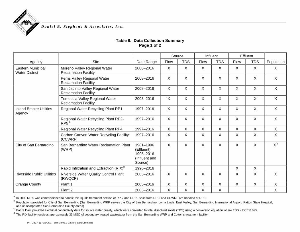
Table 6. Data Collection Summary Page 1 of 2
a In 2002 RP-5 was commissioned to handle the liquids treatment section of RP-2 and RP-2. Solid from RP-5 and CCWRF are handled at RP-2. b Population provided for City of San Bernardino (San Bernardino WRP serves the City of San Bernardino, Loma Linda, East Valley, San Bernardino International Airport, Patton State Hospital,
and unincorporated San Bernardino County areas) c Padre Dam provided electrical conductivity data for source water quality, which were converted to total dissolved solids (TDS) using a conversion equation where TDS = EC * 0.625. d The RIX facility receives approximately 33 MGD of secondary treated wastewater from the San Bernardino WRP and Colton’s treatment facility.
P:\_DB17-1179\SCSC Tech Memo.3-18\T06_DataCllctn.doc
D a n i e l B . S t e p h e n s & A s s o c i a t e s , I n c .
Source Influent Effluent Agency Site Date Range Flow TDS Flow TDS Flow TDS Population
Eastern Municipal Water District
Moreno Valley Regional Water Reclamation Facility
2008–2016 X X X X X X X
Perris Valley Regional Water Reclamation Facility
2008–2016 X X X X X X X
San Jacinto Valley Regional Water Reclamation Facility
2008–2016 X X X X X X X
Temecula Valley Regional Water Reclamation Facility
2008–2016 X X X X X X X
Inland Empire Utilities Agency
Regional Water Recycling Plant RP1 1997–2016 X X X X X X X
Regional Water Recycling Plant RP2-RP5 a
1997–2016 X X X X X X X
Regional Water Recycling Plant RP4 1997–2016 X X X X X X X Carbon Canyon Water Recycling Facility
(CCWRF) 1997–2016 X X X X X X X
City of San Bernardino San Bernardino Water Reclamation Plant (WRP)
1981–1996 (Effluent) 1995–2016 (Influent and Source)
X X X X X X X b
Rapid Infiltration and Extraction (RIX)b 1996–2016 X X Riverside Public Utilities Riverside Water Quality Control Plant
(RWQCP) 2003–2016 X X X X X X X
Orange County Plant 1 2003–2016 X X X X X X X Plant 2 2003–2016 X X X X X
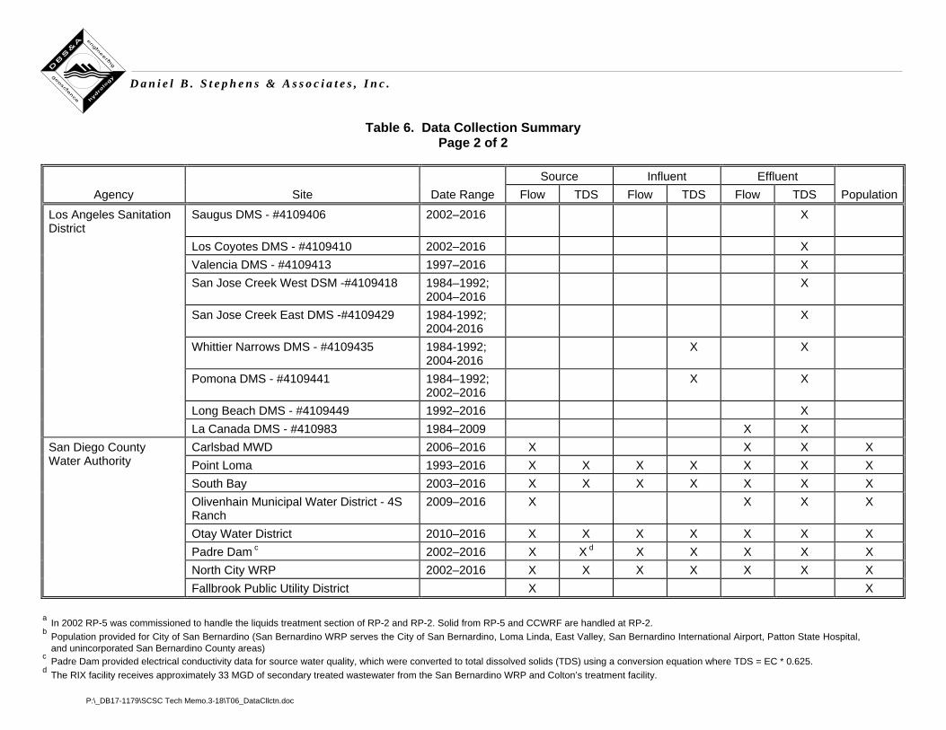
Table 6. Data Collection Summary Page 2 of 2
a In 2002 RP-5 was commissioned to handle the liquids treatment section of RP-2 and RP-2. Solid from RP-5 and CCWRF are handled at RP-2. b Population provided for City of San Bernardino (San Bernardino WRP serves the City of San Bernardino, Loma Linda, East Valley, San Bernardino International Airport, Patton State Hospital,
and unincorporated San Bernardino County areas) c Padre Dam provided electrical conductivity data for source water quality, which were converted to total dissolved solids (TDS) using a conversion equation where TDS = EC * 0.625. d The RIX facility receives approximately 33 MGD of secondary treated wastewater from the San Bernardino WRP and Colton’s treatment facility.
P:\_DB17-1179\SCSC Tech Memo.3-18\T06_DataCllctn.doc
D a n i e l B . S t e p h e n s & A s s o c i a t e s , I n c .
Source Influent Effluent Agency Site Date Range Flow TDS Flow TDS Flow TDS Population
Los Angeles Sanitation District
Saugus DMS - #4109406 2002–2016 X
Los Coyotes DMS - #4109410 2002–2016 X Valencia DMS - #4109413 1997–2016 X San Jose Creek West DSM -#4109418 1984–1992;
2004–2016 X
San Jose Creek East DMS -#4109429 1984-1992; 2004-2016
X
Whittier Narrows DMS - #4109435 1984-1992; 2004-2016
X X
Pomona DMS - #4109441 1984–1992; 2002–2016
X X
Long Beach DMS - #4109449 1992–2016 X La Canada DMS - #410983 1984–2009 X X San Diego County Water Authority
Carlsbad MWD 2006–2016 X X X X Point Loma 1993–2016 X X X X X X X South Bay 2003–2016 X X X X X X X Olivenhain Municipal Water District - 4S Ranch
2009–2016 X X X X
Otay Water District 2010–2016 X X X X X X X Padre Dam c 2002–2016 X X d X X X X X North City WRP 2002–2016 X X X X X X X Fallbrook Public Utility District X X
P:\_DB17-1179\SCSC Tech Memo.3-18\Final_330_TF.docx 17
D a n i e l B . S t e p h e n s & A s s o c i a t e s , I n c .
2.2 Eastern Municipal Water District
EMWD provides a significant portion of the water supply within their service area, and treats all
wastewater for reuse for beneficial purposes at five regional water reclamation facilities that
treat approximately 46 mgd of wastewater for nearly 800,000 residents. The five water
reclamation facilities include Moreno Valley, Perris Valley, San Jacinto Valley, Temecula Valley,
and Sun City. All flows from Sun City are diverted to Perris Valley; therefore, for this study,
these two WWTPs will be treated as one WWTP. Influent and effluent water quality data were
provided from 1993 to 2016, while source water quality was reported from 2008 to 2016.
A common operational practice for agencies with multiple treatment plants is to divert flows as
needed to ensure compliance of discharge permit requirements. Such flow divergences affect
the calculations of per capita water use. EMWD had two periods of significant construction
activity where there was extensive flow diversion. In the early 2000s, flows normally allocated
for Moreno Valley WWTP were diverted to Perris Valley WWTP. Beginning in 2012, flows
normally directed for San Jacinto Valley WWTP were diverted to Perris Valley WWTP. In
addition to the analysis of the individual sewersheds, a “combined sewershed” analysis was
performed, where the flows for each WWTP are summed together for a total flow, and influent
TDS concentrations are estimated using a volume-weighted average. This combined
sewershed approach accounts for the variations in flow divergence and other anomalies.
2.3 Inland Empire Utilities Agency
IEUA is a wholesale imported water provider, the regional wastewater treatment agency, and
the regional recycled water distributor, with nine member agencies: Chino, Chino Hills,
Cucamonga Valley Water District, Fontana, Fontana Water Company, Montclair, Monte Vista
Water District, Ontario, and Upland. IEUA serves 825,000 people and treats about 60 mgd of
wastewater. IEUA provided data for five treatment facilities: RP1, RP2, RP4, RP5, and
CCWRF. In March 2004, RP2 was taken out of service and RP5 was commissioned in its
place. Therefore, in this study, RP2 and RP5 will be treated as one system.
P:\_DB17-1179\SCSC Tech Memo.3-18\Final_330_TF.docx 18
D a n i e l B . S t e p h e n s & A s s o c i a t e s , I n c .
IEUA developed a residential SRWS removal rebate program with three main objectives: (1) to
achieve water savings, (2) to reduce salinity contributions to WWTPs, and (3) to raise
awareness about the importance of local water supplies and the need for water conservation
and reduction of salinity in recycled water (IEUA, 2012). IEUA and its member agencies
determined that the best option for regulating the use of SRWS is to prohibit the future
installation of these devices and to establish a voluntary rebate program for removal of existing
SRWS. Between 2008 and 2012, IEUA adopted a voluntary rebate program and the results of
this program are reported in a 2012 final report (IEUA, 2012).
2.4 Orange County Sanitation District/Orange County Water District
OCSD collects and treats wastewater from central and northwest Orange County from a
population of approximately 2.5 million people, and treats an average of 184 mgd of
wastewater. There are two treatment plants; in 2016, approximately 117 mgd was treated at
Plant No. 1 and 67 mgd was treated at Plant No. 2. Influent water quality data were provided
and used for Plant No. 1 only for the following reasons:
• Plant No. 2 receives approximately 30 percent of its total flow from the Inland Empire
Brine Line, a gravity pipeline that receives non-reclaimable wastewater from the Santa
Ana River watershed upstream of Orange County and includes flows from industrial
dischargers and desalination facilities. The Inland Empire Brine Line provides the
facilities for exporting salt from inland areas to the ocean (SAWPA, 2018).
• Some sewer lines in the Plant No. 2 sewershed have challenges with infiltration of
brackish shallow groundwater.
• Plant No. 2 receives brine and backwash water from Plant No. 1.
• Plant No. 2 discharges to the ocean and does not have permit limits for TDS.
OCSD keeps records of permitted discharges received by Plant No. 1, and which account for
approximately 2.5 percent of the total flow. The TDS concentrations listed below from the
permitted discharges illustrate that there are sources of high TDS concentration that are not
directly accounted for in the analysis; these include, but are not limited to, the following:
P:\_DB17-1179\SCSC Tech Memo.3-18\Final_330_TF.docx 19
D a n i e l B . S t e p h e n s & A s s o c i a t e s , I n c .
• City of Tustin Water Services (17th St): 5,500 mg/L
• City of Tustin Water Services (Main St): 9,300 mg/L
• Coca-Cola Company-Anaheim Water Plant: 1,700 mg/L
• Irvine Ranch Water District: 4,900 mg/L
• Mesa Water District: 1,700 mg/L
• Weidemann Water Conditioner, Inc.: 15,000 mg/L
To maximize OCWD’s Groundwater Replenishment System, some flows are diverted from Plant
No. 2 to Plant No. 1. Because of the flow diversion there is an apparent increase in the
calculated per capita water use at Plant No. 1 (see Section 3.1 for the calculation used in this
study for indoor per capita water), which is inconsistent with general declines in per capita water
use demonstrated from both plants. To better represent per capita water use in Orange County,
total influent flows for Plant No. 1 and Plant No. 2 were used in place of influent flow solely from
Plant No. 1. For the water quality analysis, TDS concentrations were used only from Plant
No. 1. There is a long and continuous record of effluent TDS concentration data; however,
influent TDS concentration data for Plant No. 1 are limited. TDS concentration data for source
water were provided on an annual basis instead of a monthly basis.
2.5 San Diego County Water Authority
SDCWA is a wholesale water supplier for 24 retail water agencies throughout San Diego
County. Population data were provided for each of the 24 member agencies. There are 28
treatment facilities within the county. The largest treatment network, the Metropolitan Sewerage
System, serves the greater San Diego area, has a population of approximately 2.2 million, and
overlies all or portions of nine of the retail water agencies generating approximately 180 mgd of
wastewater. The WWTPs in this service area include the North City Water Reclamation Plant
(WRP), South Bay WRP, and Point Loma WWTP. The North City and South Bay treatment
facilities are inland and send some of their effluent flow to Point Loma, which discharges to the
ocean. Due to the ability to divert flows to Point Loma WWTP, these three facilities were
analyzed as a combined average, similar to EMWD and IEUA. However, the influent TDS at
Point Loma is nearly 1,000 mg/L greater than that at both North City WRP and South Bay WRP,
which makes the apparent IFU in the combined analysis much higher than literature values.
P:\_DB17-1179\SCSC Tech Memo.3-18\Final_330_TF.docx 20
D a n i e l B . S t e p h e n s & A s s o c i a t e s , I n c .
The higher IFU can likely be attributed to the brine discharge from North City WRP and South
Bay WRP, as well as the proximity to the ocean (sea water intrusion near coastal pipes and
facilities).
Two of the smaller facilities—Otay and Padre Dam—were also analyzed independently. Padre
Dam Municipal Water District (PDMWD) collects wastewater from Santee and parts of El Cajon
and Lakeside; on average, 40 percent of the wastewater collected is processed in the Padre
Dam water recycling facility, while the remainder is sent to the City of San Diego’s metropolitan
wastewater system, where it is treated at the Point Loma facility. Source water quality for Padre
Dam was reported as electrical conductivity (EC) and was converted to TDS by PDMWD staff
by multiplying the EC by 0.625. Effective January 1, 2007, Lakeside Water District detached
from PDMWD, at which time the reported population in the sewershed declined by
35,500 people and continued a gradual decline through 2016. Otay Water District provides
sewer services to the northern portion of the district, which represents approximately 11 percent
of the total service area.
2.6 Sanitation Districts of Los Angeles County
LACSD has three major water reclamation areas, Antelope Valley WRPs (Lancaster and
Palmdale facilities), Santa Clarita Valley WRPs (Saugus and Valencia facilities), and the Joint
Outfall System (JOS) which include the Joint Water Pollution Control Plant (JWPCP), La
Cañada, Long Beach, Los Coyotes, Pomona, San Jose Creek, and Whittier Narrows Water
WRPs. The JWPCP is the only facility that discharges to the ocean. The JOS facilities are
primarily reuse plants providing water for non-potable reuse and groundwater recharge. The
data LACSD reported was limited to effluent TDS data for the Santa Clarita Valley WRPs and
the JOS facilities. The La Cañada and Long Beach facilities have the longest continuous
dataset in this study, extending back to 1984 and 1992, respectively. San Jose Creek, Whittier
Narrows, and the Pomona facilities also have data extending back to 1984; however, each of
these datasets has a 10-year data gap from the early 1990s to the early 2000s.
Extensive work has been done in the Santa Clarita Valley to reduce discharge chloride
concentrations by removing SRWS units in the area. In 2002, LACSD produced the first
P:\_DB17-1179\SCSC Tech Memo.3-18\Final_330_TF.docx 21
D a n i e l B . S t e p h e n s & A s s o c i a t e s , I n c .
comprehensive chloride source report for the Santa Clarita Valley, which includes an estimate of
the contribution from SRWS units (LACSD, 2002). LACSD provided annual chloride source
identification/reduction, pollution prevention, and public outreach plans from 2005 to 2014. The
2014 report summarizes the policies in place to reduce SRWS. In short, the Santa Clarita
Valley Sanitation District (SCVSD) took the following policy actions to reduce the number of
SRWS in their service area:
• March 2003 SRWS installation ban ordinance takes effect
• November 2005 Voluntary Phase I Rebate Program
• May 2007 Voluntary Phase II Rebate Program
• January 2009 mandatory ordinance banning SRWS
• August 2011 Ordinance Enforcement Program
The 2014 report also provides an estimation of the number of SRWS units remaining in the
system between 2002 and 2013 (LACSD, 2014), which is used to calculate the TDS contribution
in Section 3.4.
2.7 City of San Bernardino
The San Bernardino Municipal Water Department operates a 33 mgd regional secondary
treatment facility that provides services for City of San Bernardino, Loma Linda, East Valley,
San Bernardino International Airport, Patton State Hospital, and unincorporated San Bernardino
County areas. The secondary treated wastewater is then discharged to an off-site tertiary
treatment system in Rialto, the rapid infiltration and extraction facility (RIX). RIX also receives
treated wastewater from Colton’s WRP. Data from San Bernardino accounts for the influent
TDS and flows coming into the San Bernardino treatment facility and the effluent TDS and flows
from RIX. The data do not account for the influent flows from Colton’s WRP. Not all of the
corresponding population data needed for the analysis were provided.
P:\_DB17-1179\SCSC Tech Memo.3-18\Final_330_TF.docx 22
D a n i e l B . S t e p h e n s & A s s o c i a t e s , I n c .
2.8 Riverside Public Utilities
The City of Riverside Public Works department operates and maintains a wastewater collection
system for more than 300,000 people within the City of Riverside and the surrounding areas.
Four main branches come to the Riverside Regional Water Quality Control Plant (RWQCP) from
Riverside, Jurupa, and Rubidoux. Riverside Public Utilities (RPU) provided population data,
source TDS data for the City of Riverside, and influent flow and concentration data for the two
main branches that reflect the contribution from the City of Riverside.
P:\_DB17-1179\SCSC Tech Memo.3-18\Final_330_TF.docx 23
D a n i e l B . S t e p h e n s & A s s o c i a t e s , I n c .
3. Analysis and Results
This analysis considered a series of 12 research questions, the purpose of which is to provide a
quantitative understanding of the relationships among variables such as salt concentrations in
municipal influent and treated effluent, impact of water softener devices on salt concentrations
in influent, drought, and implementation of conservation practices that reduce per capita water
use. The potential link between these various factors is important in predicting how salinity
relative to water use may continue to change in the future. The data presented in the body of
the report were selected as the clearest examples for answering the research questions.
Detailed trends and statistical analysis and can be found in Appendices A and B.
3.1 How has indoor per capita water use changed over time? What are the water quality implications if the trend continues for the next 20 years?
Population in California is on the rise; it has doubled in just the last 45 years and is expected to
reach 50 million by 2050 (PPIC, 2017). Population in MWDSC’s service area rose from
16.8 million to 18.7 million from 2000 to 2015 (Figure 2) (MWDSC, 2016; California Department
of Finance, 2017). Note that even though the population increased significantly in this 15-year
period, the total water supplied was flat or trending down; from 2000 to 2015, the potable water
demands for 1.9 million additional people were met with the same total water supply, largely as
a result of conservation efforts, increased stormwater capture, and increased reuse of recycled
water, thereby decreasing the gross per capita water use in Southern California. This
population growth for MWDSC (estimated at 180,000 per year, or about 1 percent) will continue
to put significant pressure on water supplies in the region.
Indoor water use for this study is equivalent to the influent flow to a WWTP. Indoor per capita
water use is calculated by dividing the influent flow by the population of the treatment plant
service area. SCSC member agencies report indoor per capita water use in water master
plans. While the calculations of per capita use are often very similar to those of the member
agencies, there may be some discrepancies in how these numbers are calculated (such as
service areas boundaries used for population data). Local agencies can often produce more
precise estimates of indoor per capita water use than those generated in this report. Indoor per
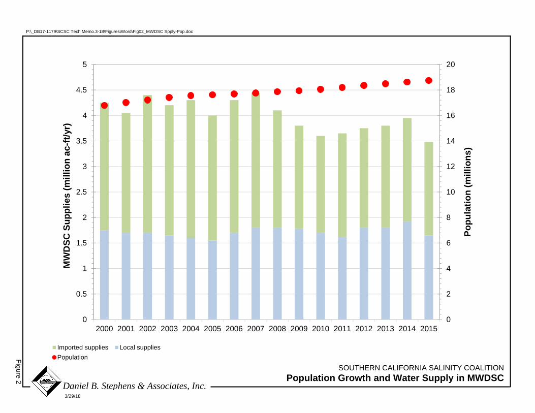
0
2
4
6
8
10
12
14
16
18
20
0
0.5
1
1.5
2
2.5
3
3.5
4
4.5
5
2000 2001 2002 2003 2004 2005 2006 2007 2008 2009 2010 2011 2012 2013 2014 2015
Popu
latio
n (m
illio
ns)
MW
DSC
Sup
plie
s (m
illio
n ac
-ft/y
r)
Imported supplies Local suppliesPopulation
SOUTHERN CALIFORNIA SALINITY COALITION Population Growth and Water Supply in MWDSC
Figure 2
3/29/18
P:\_DB17-1179\SCSC Tech Memo.3-18\Figures\Word\Fig02_MWDSC Spply-Pop.doc
Daniel B. Stephens & Associates, Inc.
P:\_DB17-1179\SCSC Tech Memo.3-18\Final_330_TF.docx 25
D a n i e l B . S t e p h e n s & A s s o c i a t e s , I n c .
capita calculations made in this study are estimates and are primarily used to represent relative
trends for each sewershed.
Using the method described above for calculating indoor per capita water, there has been a
general decrease over the past decades, from a range of 80 to 110 gpcd in the 1990s to a
range of 50 to 75 gpcd by 2016, as shown in Figure 3.
Under current proposed legislation, California residences are expected to reduce per capita
water use to 55 gpcd by 2025 (AB-968 Section 10608.25). Some members of SCSC have met
this objective and suspect that they have reached a reasonable limit for indoor conservation
measures, beyond which it may be unrealistic to achieve lower per capita indoor water use.
These groups will likely see a change in indoor water use from a downward trend to a flat trend.
Service areas that have not reached this 55 gpcd goal will likely continue to see a downward
trend in per capita water use. The implication for continued decrease in per capita water use is
an estimated 1.2 to 1.7 mg/L increase in WWTP influent TDS for every 1.0 gpcd decrease in
indoor water use (see Section 4 for more details).
3.2 How has the volume‐weighted average concentration of TDS in municipal influent changed over time? What are the water quality implications if the trend continues for the next 20 years?
There are 14 WWTPs with influent TDS data and 26 with effluent TDS data. Of the 14 WWTPs
with influent TDS data, 9 have upward trends of TDS, 4 have flat trends, and 1 has a downward
trend. Influent and effluent trends are generally closely correlated as shown in Appendix A.
The WWTPs that do not have influent TDS data were likely to have similar TDS trends
compared to their observed effluent TDS trends. Of the 26 WWTPs that have effluent TDS
data, 15 have an upward trend in TDS, 7 have no trend, and 4 have a downward trend in TDS;
nearly 60 percent of the WWTPs had increasing TDS trends.
If upward TDS concentration trends continue, more wastewater agencies will approach or
exceed discharge permit limits. In some cases, desalination treatment facilities may be required
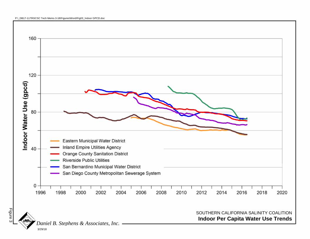
SOUTHERN CALIFORNIA SALINITY COALITION Indoor Per Capita Water Use Trends
Figure 3
3/29/18
P:\_DB17-1179\SCSC Tech Memo.3-18\Figures\Word\Fig03_Indoor GPCD.doc
Daniel B. Stephens & Associates, Inc.
P:\_DB17-1179\SCSC Tech Memo.3-18\Final_330_TF.docx 27
D a n i e l B . S t e p h e n s & A s s o c i a t e s , I n c .
to mitigate the increasing levels of TDS. As more agencies move toward the use of recycled
water, the quality of the effluent water will impact the quality of the recycled water.
3.3 How has the residential/commercial per capita “increment from use” for TDS changed over time? What are the water quality implications if the trend continues for the next 20 years?
IFU is defined as the difference between influent TDS and source TDS. IFU values for the
sewersheds analyzed in this study fall within the range of literature values: 200 to 400 mg/L. In
other words, if the volume-weighted source water TDS concentration is 350 mg/L, the TDS
concentration of WWTP influent will be between 550 and 750 mg/L, with the added salt from
indoor uses. The statistical models estimate an increase in effluent TDS between 1.2 and
1.7 mg/L for every 1.0 gpcd decrease in indoor water use. A more in-depth discussion of the
statistical analysis is provided in Section 4.
OCWD/OCSD and SDCWA are exceptions to the normal range of IFU, and had values that far
exceeded typically literature values, with IFU values exceeding 1,000 mg/L. Both OCSD and
SDCWA are coastal agencies, and sea water infiltration to sewer lines in low-elevation areas is
one probable cause of higher IFU values. As described in Section 2, Orange County permits
industrial discharges with high TDS concentrations that exceed the typical contribution of TDS
from human excretion and gray water disposal. Similarly, the Point Loma WRP in the San
Diego Metropolitan Sewerage System service area receives brine from North City and South
Bay WRPs.
3.4 What proportion of the increase in average per capita increment from use can be attributed to widespread implementation of low‐flow plumbing fixtures and appliances?
Urban water conservation has gained much attention since the 1976/1977 drought in California.
Indoor water conservation measures employed in the mid- to late-1970s include the installation
of “low-flow faucet aerators, low-flow shower heads or flow restrictors, and ‘water dams’ or
P:\_DB17-1179\SCSC Tech Memo.3-18\Final_330_TF.docx 28
D a n i e l B . S t e p h e n s & A s s o c i a t e s , I n c .
plastic bottles in toilet tanks to reduce the amount of water used for flushing” (U.S. EPA, 1980).
Commonly used devises for indoor conservation currently include ultra-low flow toilets (ULFT),
high efficiency toilets (HET), high-efficiency clothes washers (HECW), and low-flow
showerheads.
The two primary methods for implementing low-flow plumbing fixtures are through changes to
the plumbing codes (difficult to measure and keep records) and through conservation incentive
programs, such as buy-back rebate programs. Estimates of conservation were reported for
active installation/replacement of low-flow fixtures through incentive programs. Water saved
through passive measures, (e.g., ordinances and building code changes) were not provided for
this report. OCWD, SDCWA, and RPU provided records of the implementation of low‐flow
plumbing fixtures and appliances for both indoor and outdoor devices.
Using Orange County as an example, the impact of these devices over time can be measured.
OCWD recorded the number of units installed through local conservation programs and
provided the cumulative number of indoor devices installed, HECW, HET, and ULFT. The
number of installed devices compared to the indoor water use (in mgd) over that time period is
shown in Figure 4. This figure does not include water used for showers, as only totals were
provided instead of annual records. In 2016, the amount of indoor water saved through active
conservation is approximately 6.3 gpcd. Using the increase from IFU values introduced in
Question 2, there would be an increase in TDS in the range of 7.6 to 10.7 mg/L.
In 2016, the annual water savings from the installation and use of HECW, HET, ULFT, and low-
flow showerheads are:
• HECW: 3,800 acre-feet, or approximately 1,300 million gallons
• HET: 2,200 acre-feet, or approximately 700 million gallons
• ULFT: 13,500 acre-feet, or approximately 4,400 million gallons
• Showers: 1,700 acre-feet, or approximately 500 million gallons
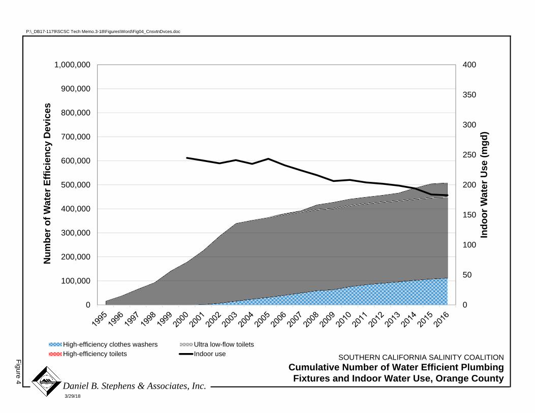
0
50
100
150
200
250
300
350
400
0
100,000
200,000
300,000
400,000
500,000
600,000
700,000
800,000
900,000
1,000,000
Indo
or W
ater
Use
(mgd
)
Num
ber o
f Wat
er E
ffici
ency
Dev
ices
High-efficiency clothes washers Ultra low-flow toiletsHigh-efficiency toilets Indoor use
SOUTHERN CALIFORNIA SALINITY COALITION Cumulative Number of Water Efficient Plumbing Fixtures and Indoor Water Use, Orange County
Figure 4
3/29/18
P:\_DB17-1179\SCSC Tech Memo.3-18\Figures\Word\Fig04_CnsvtnDvces.doc
Daniel B. Stephens & Associates, Inc.
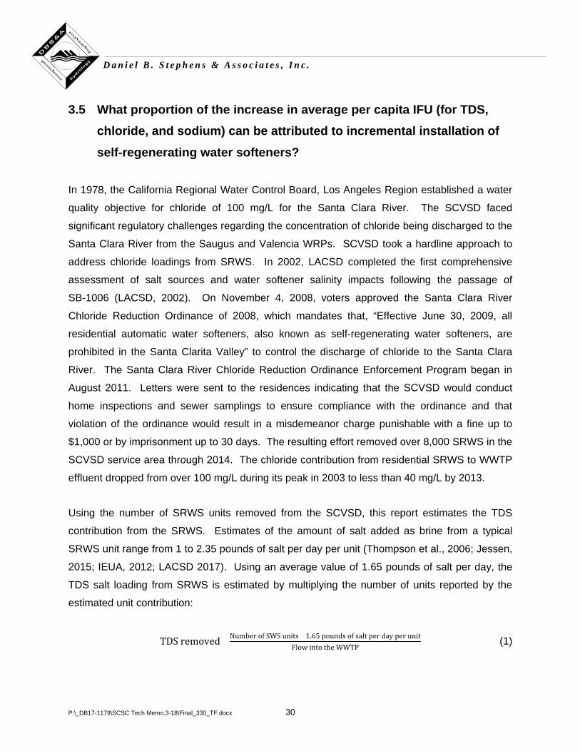
P:\_DB17-1179\SCSC Tech Memo.3-18\Final_330_TF.docx 30
D a n i e l B . S t e p h e n s & A s s o c i a t e s , I n c .
3.5 What proportion of the increase in average per capita IFU (for TDS,
chloride, and sodium) can be attributed to incremental installation of self‐regenerating water softeners?
In 1978, the California Regional Water Control Board, Los Angeles Region established a water
quality objective for chloride of 100 mg/L for the Santa Clara River. The SCVSD faced
significant regulatory challenges regarding the concentration of chloride being discharged to the
Santa Clara River from the Saugus and Valencia WRPs. SCVSD took a hardline approach to
address chloride loadings from SRWS. In 2002, LACSD completed the first comprehensive
assessment of salt sources and water softener salinity impacts following the passage of
SB-1006 (LACSD, 2002). On November 4, 2008, voters approved the Santa Clara River
Chloride Reduction Ordinance of 2008, which mandates that, “Effective June 30, 2009, all
residential automatic water softeners, also known as self-regenerating water softeners, are
prohibited in the Santa Clarita Valley” to control the discharge of chloride to the Santa Clara
River. The Santa Clara River Chloride Reduction Ordinance Enforcement Program began in
August 2011. Letters were sent to the residences indicating that the SCVSD would conduct
home inspections and sewer samplings to ensure compliance with the ordinance and that
violation of the ordinance would result in a misdemeanor charge punishable with a fine up to
$1,000 or by imprisonment up to 30 days. The resulting effort removed over 8,000 SRWS in the
SCVSD service area through 2014. The chloride contribution from residential SRWS to WWTP
effluent dropped from over 100 mg/L during its peak in 2003 to less than 40 mg/L by 2013.
Using the number of SRWS units removed from the SCVSD, this report estimates the TDS
contribution from the SRWS. Estimates of the amount of salt added as brine from a typical
SRWS unit range from 1 to 2.35 pounds of salt per day per unit (Thompson et al., 2006; Jessen,
2015; IEUA, 2012; LACSD 2017). Using an average value of 1.65 pounds of salt per day, the
TDS salt loading from SRWS is estimated by multiplying the number of units reported by the
estimated unit contribution:
TDS removed= Number of SWS units ×1.65 pounds of salt per day per unitFlow into the WWTP
(1)
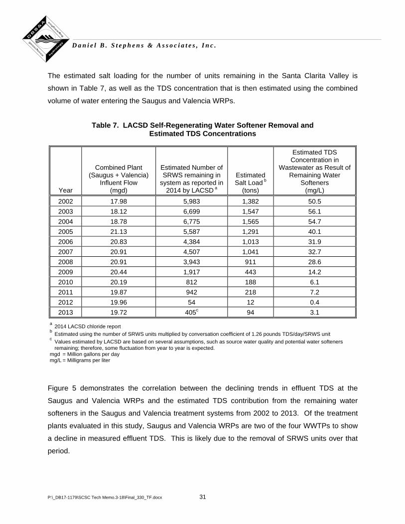
P:\_DB17-1179\SCSC Tech Memo.3-18\Final_330_TF.docx 31
D a n i e l B . S t e p h e n s & A s s o c i a t e s , I n c .
The estimated salt loading for the number of units remaining in the Santa Clarita Valley is
shown in Table 7, as well as the TDS concentration that is then estimated using the combined
volume of water entering the Saugus and Valencia WRPs.
Table 7. LACSD Self-Regenerating Water Softener Removal and Estimated TDS Concentrations
Year
Combined Plant (Saugus + Valencia)
Influent Flow (mgd)
Estimated Number of SRWS remaining in
system as reported in 2014 by LACSD a
Estimated Salt Load b
(tons)
Estimated TDS Concentration in
Wastewater as Result of Remaining Water
Softeners (mg/L)
2002 17.98 5,983 1,382 50.5 2003 18.12 6,699 1,547 56.1 2004 18.78 6,775 1,565 54.7 2005 21.13 5,587 1,291 40.1 2006 20.83 4,384 1,013 31.9 2007 20.91 4,507 1,041 32.7 2008 20.91 3,943 911 28.6 2009 20.44 1,917 443 14.2 2010 20.19 812 188 6.1 2011 19.87 942 218 7.2 2012 19.96 54 12 0.4 2013 19.72 405c 94 3.1
a 2014 LACSD chloride report b Estimated using the number of SRWS units multiplied by conversation coefficient of 1.26 pounds TDS/day/SRWS unit c Values estimated by LACSD are based on several assumptions, such as source water quality and potential water softeners
remaining; therefore, some fluctuation from year to year is expected. mgd = Million gallons per day mg/L = Milligrams per liter
Figure 5 demonstrates the correlation between the declining trends in effluent TDS at the
Saugus and Valencia WRPs and the estimated TDS contribution from the remaining water
softeners in the Saugus and Valencia treatment systems from 2002 to 2013. Of the treatment
plants evaluated in this study, Saugus and Valencia WRPs are two of the four WWTPs to show
a decline in measured effluent TDS. This is likely due to the removal of SRWS units over that
period.
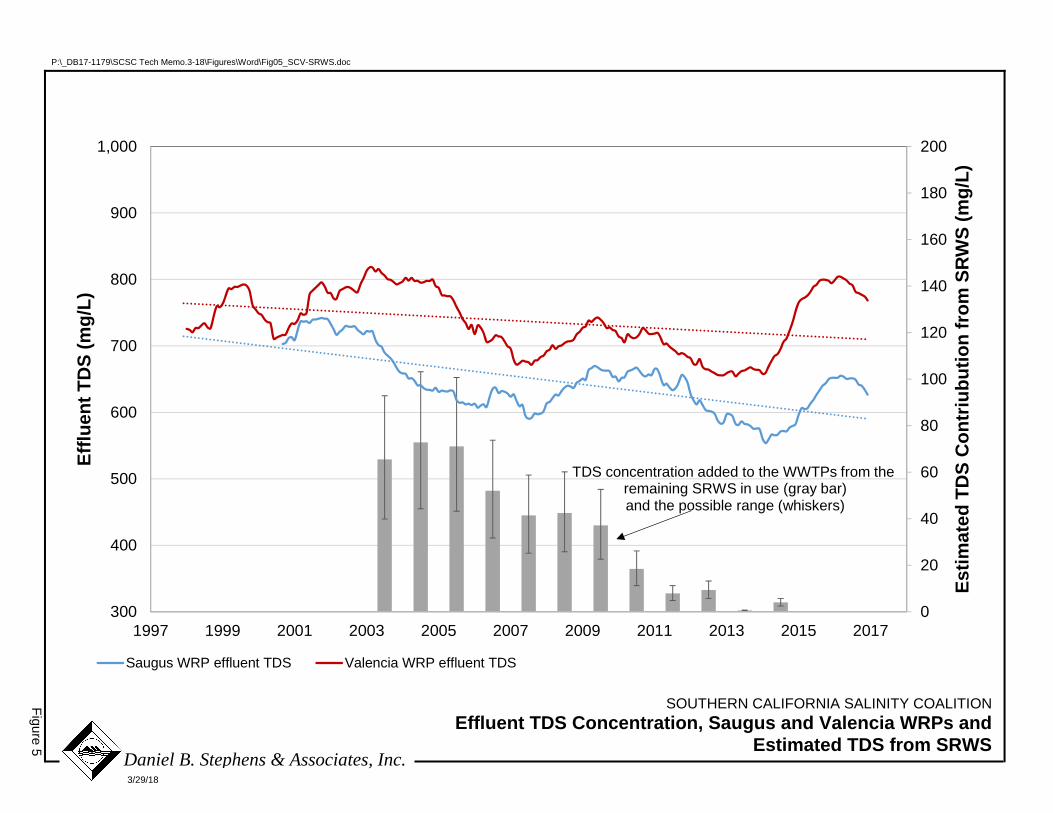
0
20
40
60
80
100
120
140
160
180
200
300
400
500
600
700
800
900
1,000
1997 1999 2001 2003 2005 2007 2009 2011 2013 2015 2017
Estim
ated
TD
S C
ontr
iubu
tion
from
SR
WS
(mg/
L)
Efflu
ent T
DS
(mg/
L)
Saugus WRP effluent TDS Valencia WRP effluent TDS
TDS concentration added to the WWTPs from the remaining SRWS in use (gray bar)and the possible range (whiskers)
SOUTHERN CALIFORNIA SALINITY COALITION Effluent TDS Concentration, Saugus and Valencia WRPs and
Estimated TDS from SRWS
Figure 5
3/29/18
P:\_DB17-1179\SCSC Tech Memo.3-18\Figures\Word\Fig05_SCV-SRWS.doc
Daniel B. Stephens & Associates, Inc.
P:\_DB17-1179\SCSC Tech Memo.3-18\Final_330_TF.docx 33
D a n i e l B . S t e p h e n s & A s s o c i a t e s , I n c .
Following the model established by LACSD, IEUA developed a residential SRWS removal
rebate program with three main objectives: (1) to achieve water savings, (2) to reduce salinity
contribution to WWTPs, and (3) to raise awareness about the importance of local water supplies
and the need for water conservation and reduction of salinity in recycled water (IEUA, 2012).
IEUA and its member agencies determined that the best option for regulating the use of SRWS
was to prohibit the future installation of these devices and to establish a voluntary rebate
program. Between 2008 and 2012, IEUA successfully removed 511 residential SRWS units; as
a result, it is estimated that a total of 236,000 pounds of salt was removed from the system
during this time period. Multiplied by the current average influent flow to treatment system of
55 mgd, the removal of these units resulted in an estimated reduction in TDS of 1.4 mg/L.
The secondary y-axis in Figure 6 shows the hypothetical salt load removed as a function of the
number of SRWS removed from the system, shown in red on the graph. For example, removing
6000 SRWS units at 1.65 pounds per day would result in the removal of a mass of salt
equivalent to 1,800 tons per year. The blue data points (SCVSD) and the green data points
(IEUA) show the resultant reduction of TDS concentrations (primary y-axis) based on their
respective flow rates: 55 mgd for IEUA and 18 to 21 mgd for SCVSD.
For example, the indoor use for SCVSD between 2003 and 2014 was 18 to 21 mgd, and it is
estimated (in blue) that due to removal of 6,000 SRWS units, the TDS concentration of water
entering the WWTP was approximately 65 mg/L less than it would have been if no SRWS had
been removed. On the other hand, IEUA has an indoor water use of approximately 55 mgd; if,
hypothetically, the agency removed the same number of SRWS, it would only reduce the
concentration by approximately 20 mg/L as shown in green.
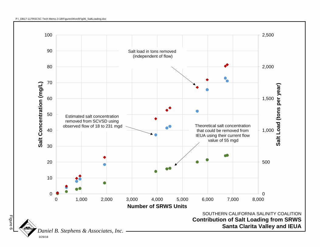
0
500
1,000
1,500
2,000
2,500
0
10
20
30
40
50
60
70
80
90
100
0 1,000 2,000 3,000 4,000 5,000 6,000 7,000 8,000
Salt
Load
(ton
s pe
r yea
r)
Salt
Con
cent
ratio
n (m
g/L)
Number of SRWS Units
Salt load in tons removed (independent of flow)
Estimated salt concentration removed from SCVSD using
observed flow of 18 to 231 mgd Theoretical salt concentration that could be removed fromIEUA using their current flow
value of 55 mgd
SOUTHERN CALIFORNIA SALINITY COALITION Contribution of Salt Loading from SRWS
Santa Clarita Valley and IEUA
Figure 6
3/29/18
P:\_DB17-1179\SCSC Tech Memo.3-18\Figures\Word\Fig06_SaltLoading.doc
Daniel B. Stephens & Associates, Inc.
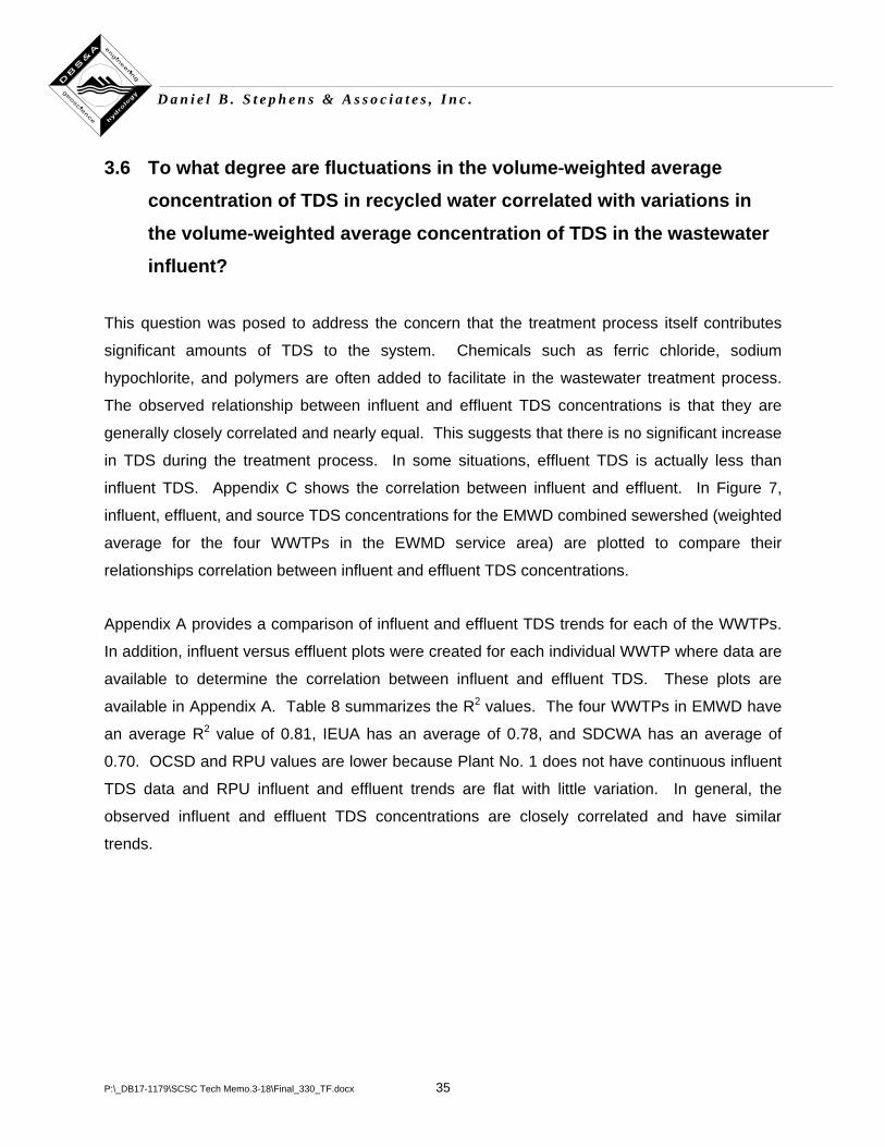
P:\_DB17-1179\SCSC Tech Memo.3-18\Final_330_TF.docx 35
D a n i e l B . S t e p h e n s & A s s o c i a t e s , I n c .
3.6 To what degree are fluctuations in the volume‐weighted average
concentration of TDS in recycled water correlated with variations in the volume‐weighted average concentration of TDS in the wastewater influent?
This question was posed to address the concern that the treatment process itself contributes
significant amounts of TDS to the system. Chemicals such as ferric chloride, sodium
hypochlorite, and polymers are often added to facilitate in the wastewater treatment process.
The observed relationship between influent and effluent TDS concentrations is that they are
generally closely correlated and nearly equal. This suggests that there is no significant increase
in TDS during the treatment process. In some situations, effluent TDS is actually less than
influent TDS. Appendix C shows the correlation between influent and effluent. In Figure 7,
influent, effluent, and source TDS concentrations for the EMWD combined sewershed (weighted
average for the four WWTPs in the EWMD service area) are plotted to compare their
relationships correlation between influent and effluent TDS concentrations.
Appendix A provides a comparison of influent and effluent TDS trends for each of the WWTPs.
In addition, influent versus effluent plots were created for each individual WWTP where data are
available to determine the correlation between influent and effluent TDS. These plots are
available in Appendix A. Table 8 summarizes the R2 values. The four WWTPs in EMWD have
an average R2 value of 0.81, IEUA has an average of 0.78, and SDCWA has an average of
0.70. OCSD and RPU values are lower because Plant No. 1 does not have continuous influent
TDS data and RPU influent and effluent trends are flat with little variation. In general, the
observed influent and effluent TDS concentrations are closely correlated and have similar
trends.
SOUTHERN CALIFORNIA SALINITY COALITION Influent, Effluent, and Source TDS Trends for EMWD
(Weighted Average of All Sewersheds)
Figure 7
3/29/18
P:\_DB17-1179\SCSC Tech Memo.3-18\Figures\Word\Fig07_EMWD-WghtdAvgs.doc
Daniel B. Stephens & Associates, Inc.
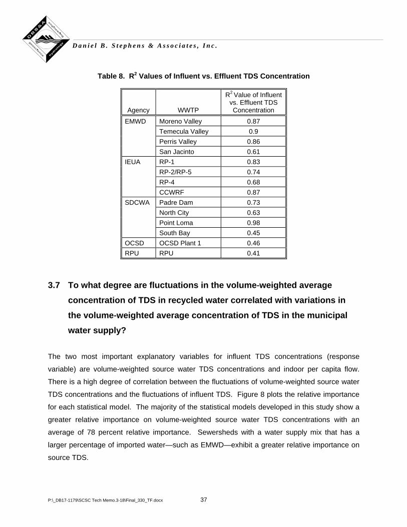
P:\_DB17-1179\SCSC Tech Memo.3-18\Final_330_TF.docx 37
D a n i e l B . S t e p h e n s & A s s o c i a t e s , I n c .
Table 8. R2 Values of Influent vs. Effluent TDS Concentration
Agency WWTP
R2 Value of Influent vs. Effluent TDS Concentration
EMWD Moreno Valley 0.87 Temecula Valley 0.9 Perris Valley 0.86 San Jacinto 0.61
IEUA RP-1 0.83 RP-2/RP-5 0.74 RP-4 0.68 CCWRF 0.87
SDCWA Padre Dam 0.73 North City 0.63 Point Loma 0.98 South Bay 0.45
OCSD OCSD Plant 1 0.46 RPU RPU 0.41
3.7 To what degree are fluctuations in the volume‐weighted average concentration of TDS in recycled water correlated with variations in the volume‐weighted average concentration of TDS in the municipal water supply?
The two most important explanatory variables for influent TDS concentrations (response
variable) are volume-weighted source water TDS concentrations and indoor per capita flow.
There is a high degree of correlation between the fluctuations of volume-weighted source water
TDS concentrations and the fluctuations of influent TDS. Figure 8 plots the relative importance
for each statistical model. The majority of the statistical models developed in this study show a
greater relative importance on volume-weighted source water TDS concentrations with an
average of 78 percent relative importance. Sewersheds with a water supply mix that has a
larger percentage of imported water—such as EMWD—exhibit a greater relative importance on
source TDS.

0
10
20
30
40
50
60
70
80
90
100
Influent Flow (GPCD) Source TDS
Rel
ativ
e Im
port
ance
(%)
EMWD Combined IEUA Combined
SDCWA Metro OCSD
SOUTHERN CALIFORNIA SALINITY COALITION Relative Importance of Influent Flow and
Source TDS Variables
Figure 8
3/29/18
P:\_DB17-1179\SCSC Tech Memo.3-18\Figures\Word\Fig08_RltvImprtnc-Vrbles.doc
Daniel B. Stephens & Associates, Inc.
P:\_DB17-1179\SCSC Tech Memo.3-18\Final_330_TF.docx 39
D a n i e l B . S t e p h e n s & A s s o c i a t e s , I n c .
3.8 To what degree do fluctuations in the volume‐weighted average
concentration of TDS in recycled water correlate with long‐term meteorological (drought) cycles?
As shown in the response to Question 7, there is a high degree of correlation between the
volume-weighted source water TDS concentrations (explanatory variable) and the effluent
discharge TDS concentrations (response variable). One of the factors influencing the quality of
source water supply water is the long-term meteorological cycles including droughts. One way
to evaluate drought is through the Palmer Drought Severity Index (PDSI) established by the
National Oceanic and Atmosphere Administration (NOAA). According to NOAA (2017):
The Palmer Drought Severity Index (PDSI) uses readily available temperature and precipitation
data to estimate relative dryness. It is a standardized index that spans –10 (dry) to +10 (wet). It
has been reasonably successful at quantifying long-term drought. As it uses temperature data
and a physical water balance model, it can capture the basic effect of global warming on drought
through changes in potential evapotranspiration. Monthly PDSI values do not capture droughts
on time scales less than about 12 months.
This analysis uses the Modified Palmer Drought Severity Index (PMDI), which is an update to
the PDSI for operational meteorological purposes (NOAA, 2017). The PMDI and PDSI have the
same values during established wet periods and droughts; however, they differ slightly when the
meteorological cycles transition from one to another. While this study focuses on WWTPs in
Southern California, a drought in Northern California can change TDS concentrations in source
water in Southern California and a drought in the Rocky Mountains can have an effect on TDS
in the Colorado River. This analysis uses the drought index for the entire state of California as a
general picture of drought conditions affecting imported and local water supply quality in
Southern California. Local drought indices will vary region to region.
Another way to analyze climatic variations is through the 8-Station Index, which compares the
annual precipitation with a 50-year average (DWR, 2018). The DWR began development of the
8-Station Index for tracking precipitation in the Northern Sierra in the 1980s. The 8-Station
Index was originally designed to be a simple index of the cumulative amount of precipitation
P:\_DB17-1179\SCSC Tech Memo.3-18\Final_330_TF.docx 40
D a n i e l B . S t e p h e n s & A s s o c i a t e s , I n c .
(rainfall and snow) that fell in the watershed of the Sacramento River Basin throughout the
water year. Stations were selected to record the average water year runoff: three stations for
the Sacramento River above the historical Red Bluff gage (Mt. Shasta City, Shasta Dam,
Mineral), three stations for the Feather-Yuba River (Brush Creek, Quincy, Sierraville), and two
for the American River (Blue Canyon and Pacific House).
The original average precipitation of the 8-Station Index, starting in the 1920s and going through
the 1980s, was 50 inches. DWR recently updated the 8-Station Index average precipitation for
the 1966-2015 period to 51.8 inches. There will be a further update in 2021 for a new 1971-
2020 50-year average).
Figure 9 compares the PMDI and 8-Station Index to surface supply water quality data for major
reservoirs and treatment facilities operated by MWDSC. Time-series TDS concentrations are
shown for Skinner Lake, Lake Mathews, Deimer WTP, and Weymouth WTP as part of the
Colorado River Aqueduct, and for Mills, Silverwood Lake, Castaic Lake, and Jensen WTP as
part of the SWP. Aside from Lake Mathews, which has a more gradual trend, all reservoirs
show similar increases in TDS during periods of drought and decreases in TDS during wet
years.
To meet water demands, water agencies maintain a portfolio including imported water and
groundwater; this mix influences how much impact climate change has on the source supply
water. For example, both EMWD and IEUA rely on a blend of groundwater and imported water;
however, EMWD receives CRA water, while IEUA only receives SWP water. In addition, IEUA
relies more heavily on groundwater than EMWD. These differences between the two service
areas are reflected in the variability in volume-weighted source water TDS concentrations.
EMWD has larger fluctuations in concentration, while IEUA is increasing only slightly and shows
a relatively smooth trend compared with EMWD.
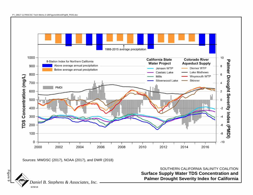
SOUTHERN CALIFORNIA SALINITY COALITION Surface Supply Water TDS Concentration and
Palmer Drought Severity Index for California
Figure 9
3/29/18
P:\_DB17-1179\SCSC Tech Memo.3-18\Figures\Word\Fig09_PDSI.doc
Daniel B. Stephens & Associates, Inc.
Sources: MWDSC (2017), NOAA (2017), and DWR (2018)
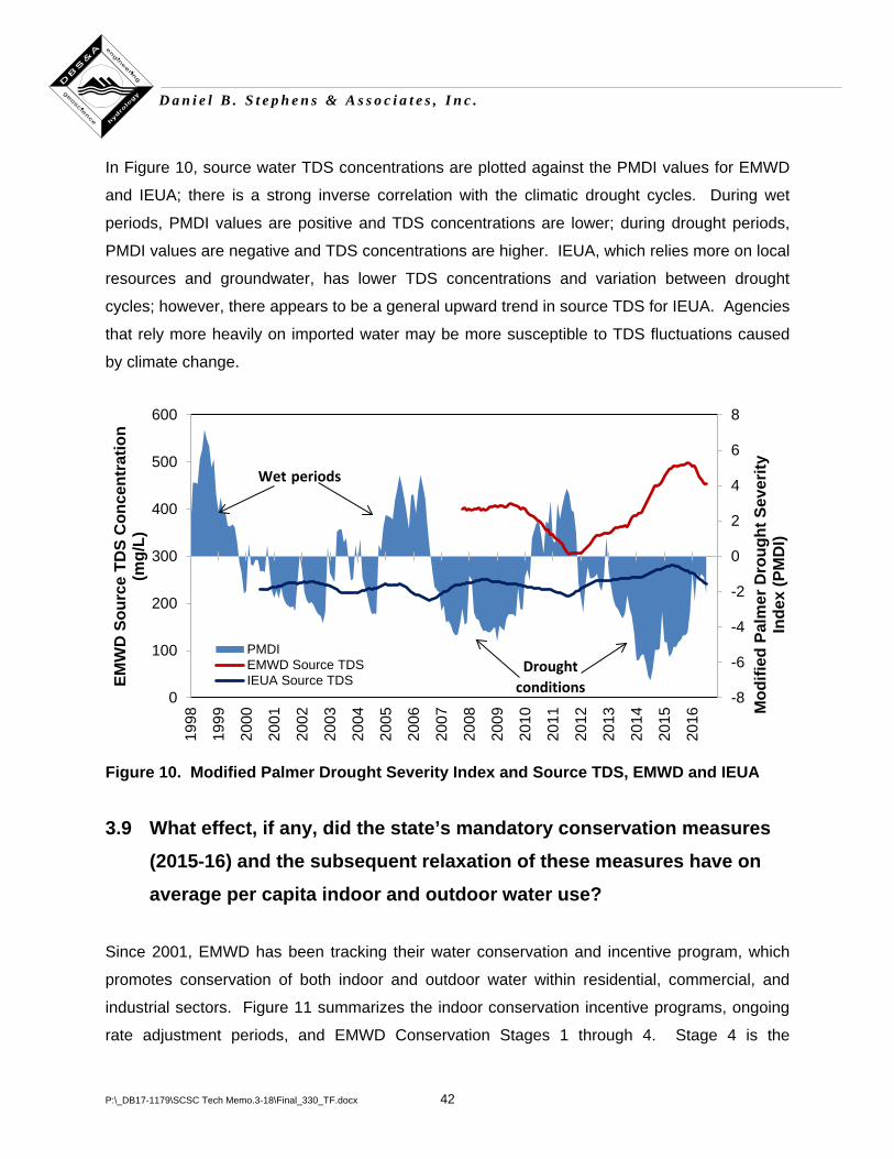
P:\_DB17-1179\SCSC Tech Memo.3-18\Final_330_TF.docx 42
D a n i e l B . S t e p h e n s & A s s o c i a t e s , I n c .
In Figure 10, source water TDS concentrations are plotted against the PMDI values for EMWD
and IEUA; there is a strong inverse correlation with the climatic drought cycles. During wet
periods, PMDI values are positive and TDS concentrations are lower; during drought periods,
PMDI values are negative and TDS concentrations are higher. IEUA, which relies more on local
resources and groundwater, has lower TDS concentrations and variation between drought
cycles; however, there appears to be a general upward trend in source TDS for IEUA. Agencies
that rely more heavily on imported water may be more susceptible to TDS fluctuations caused
by climate change.
Figure 10. Modified Palmer Drought Severity Index and Source TDS, EMWD and IEUA
3.9 What effect, if any, did the state’s mandatory conservation measures (2015‐16) and the subsequent relaxation of these measures have on average per capita indoor and outdoor water use?
Since 2001, EMWD has been tracking their water conservation and incentive program, which
promotes conservation of both indoor and outdoor water within residential, commercial, and
industrial sectors. Figure 11 summarizes the indoor conservation incentive programs, ongoing
rate adjustment periods, and EMWD Conservation Stages 1 through 4. Stage 4 is the
0
100
200
300
400
500
600
1998
1999
2000
2001
2002
2003
2004
2005
2006
2007
2008
2009
2010
2011
2012
2013
2014
2015
2016
-8
-6
-4
-2
0
2
4
6
8
EMW
D S
ourc
e TD
S C
once
ntra
tion
(mg/
L)
Mod
ified
Pal
mer
Dro
ught
Sev
erity
In
dex
(PM
DI)
PMDIEMWD Source TDSIEUA Source TDS
Wet periods
Drought conditions
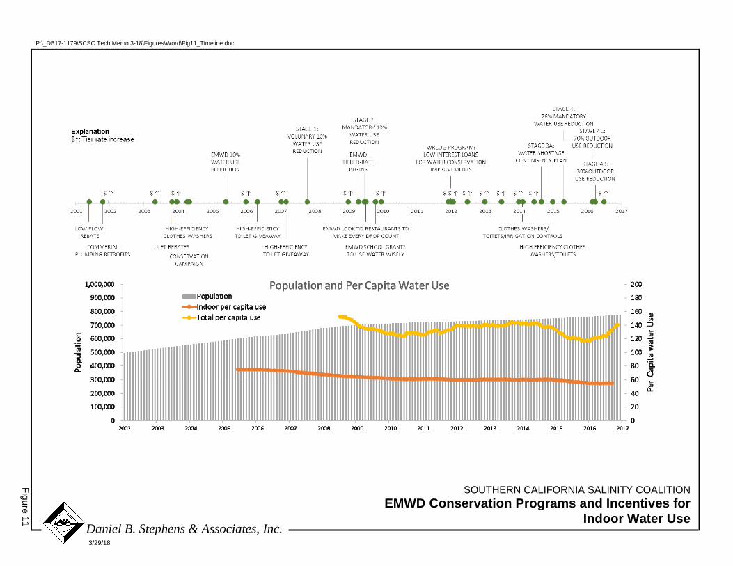
SOUTHERN CALIFORNIA SALINITY COALITION EMWD Conservation Programs and Incentives for
Indoor Water Use
Figure 11
3/29/18
P:\_DB17-1179\SCSC Tech Memo.3-18\Figures\Word\Fig11_Timeline.doc
Daniel B. Stephens & Associates, Inc.
P:\_DB17-1179\SCSC Tech Memo.3-18\Final_330_TF.docx 44
D a n i e l B . S t e p h e n s & A s s o c i a t e s , I n c .
most aggressive in terms of water conservation, and coincided with the Governor’s 2015
emergency proclamation. The timeline of conservation incentives and programs is compared to
the timeline of population growth and indoor per capita water use (dark orange) and total per
capita water use (light orange).
Figure 11 suggests that as policies are implemented and technology becomes more efficient,
consumers become more adapted to conserving water and policies made at the state level are
much more gradual than expected. There are subtle changes that occurred at certain points in
time. In particular, between 2004 and 2010 there is a general decrease in per capita indoor
water use. From 2010 to 2015, per capita indoor water use remained constant at around
60 gpcd, and in May 2015, per capita indoor water use began to decline again down to 55 gpcd
in 2016. The response to the state’s mandatory conservation measure from the 2015 executive
order to reduce water use by 25 percent statewide is more evident in total per capita water use
rapid declines following 2015 (Figure 11). Total water use includes both indoor uses such as
residential, commercial, and industrial, as well as outdoor use such as agricultural and
landscape irrigation uses.
3.10 What effect, if any, did the 2015‐16 changes in average per capita indoor water use have on the average concentration of TDS in wastewater influent and recycled water?
As described in Question 1 and Question 9, there is a gradual downward trend in indoor per
capita water use over time. Changes in average indoor per capita water use following the
mandatory conservation measures in 2015 are minimal, especially when compared with total
water use. Analysis of this particular event suggests that it was not statistically significant in
modeling influent TDS concentration changes. This is, in part, because the 12-month rolling
averages tend to smooth out short-term changes in monthly TDS concentrations.
P:\_DB17-1179\SCSC Tech Memo.3-18\Final_330_TF.docx 45
D a n i e l B . S t e p h e n s & A s s o c i a t e s , I n c .
3.11 Based on the results produced for Questions 8, 9, and 10, what are the
implications for the trends described in Questions 1, 2, and 3 if precipitation patterns over the next 20 years are drier than normal (i.e., consistent with each agency’s planning for potential climate change)?
Matrices for EMWD and IEUA (Tables 9a and 9b) were developed from the statistical models to
predict the effects of conservation and changes in source water TDS. On the top row is a range
of values for volume-weighted source water supply TDS concentrations. On the left axis of the
matrix is a range of values for indoor per capita water use. The center of the matrix shows the
model-predicted influent TDS concentrations at a given indoor per capita water use and a given
source TDS value. Supply water concentrations are dependent upon the blend of imported
water and local resources, as well as climatic changes.
As the indoor per capita use decreases, the resulting influent TDS concentration increases. The
statistical model for EMWD predicts a 1.7 mg/L increase in WWTP influent TDS for every
1.0 gpcd decrease in indoor water use, while the statistical model for IEUA predicts a 1.2 mg/L
increase in WWTP influent TDS for every 1.0 gpcd decrease in indoor water use. For example,
during the peak of the 2016 drought, TDS in the volume-weighted potable supply water for
EMWD reached 500 mg/L. At this time the indoor per capita water use was 55 gpcd, and the
resulting influent TDS was approximately 750 mg/L. As described in the response to
Question 1, there is a downward trend of indoor per capita water use, and as shown in the
matrices (Tables 9a and 9b), decreasing per capita use increases TDS concentrations. The
response to Question 8 predicts that source supply water will exhibit an increase in TDS
concentrations during drought cycles.
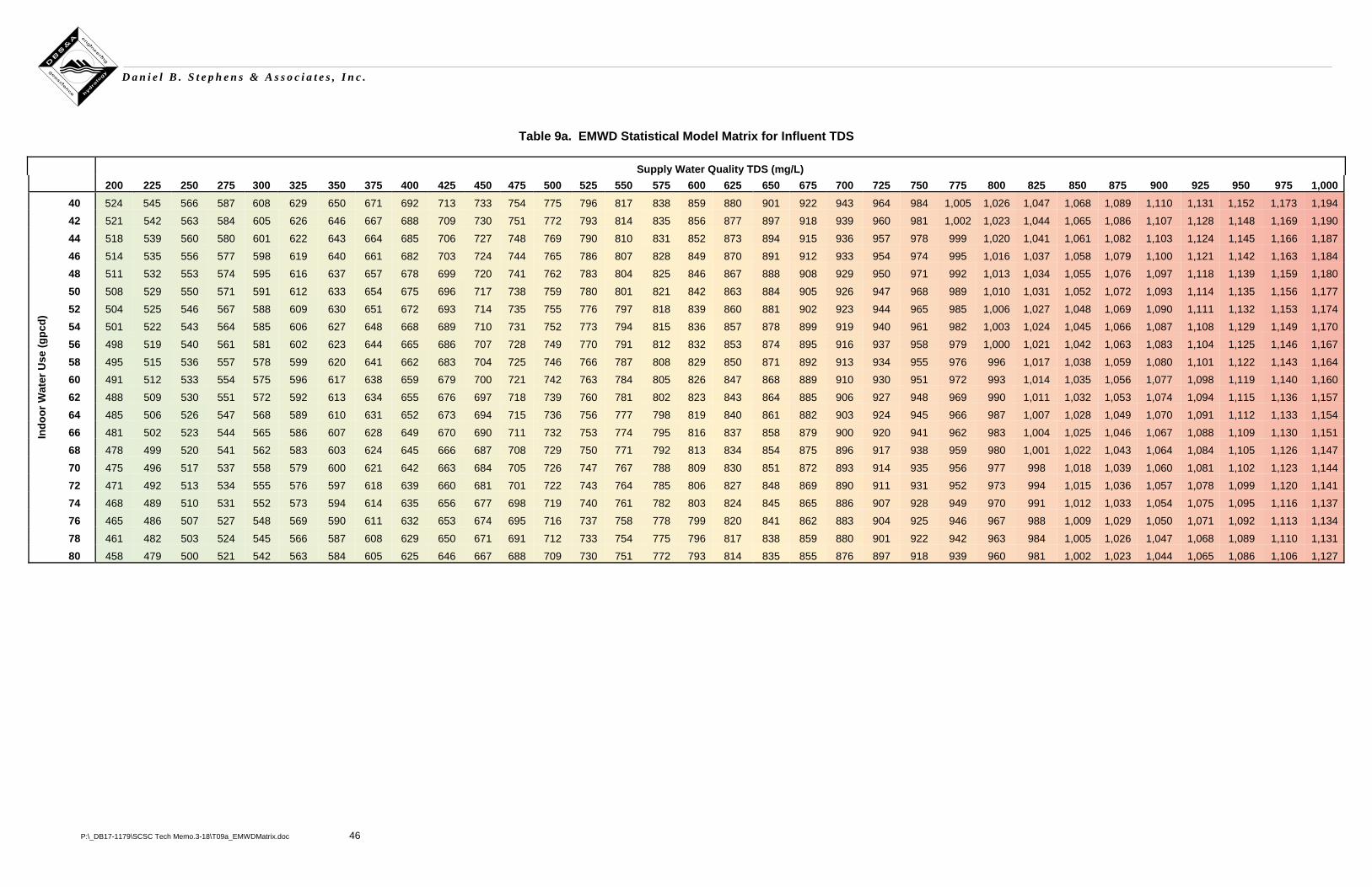
P:\_DB17-1179\SCSC Tech Memo.3-18\T09a_EMWDMatrix.doc 46
D a n i e l B . S t e p h e n s & A s s o c i a t e s , I n c .
Table 9a. EMWD Statistical Model Matrix for Influent TDS
Supply Water Quality TDS (mg/L) 200 225 250 275 300 325 350 375 400 425 450 475 500 525 550 575 600 625 650 675 700 725 750 775 800 825 850 875 900 925 950 975 1,000
Indo
or W
ater
Use
(gpc
d)
40 524 545 566 587 608 629 650 671 692 713 733 754 775 796 817 838 859 880 901 922 943 964 984 1,005 1,026 1,047 1,068 1,089 1,110 1,131 1,152 1,173 1,194 42 521 542 563 584 605 626 646 667 688 709 730 751 772 793 814 835 856 877 897 918 939 960 981 1,002 1,023 1,044 1,065 1,086 1,107 1,128 1,148 1,169 1,190 44 518 539 560 580 601 622 643 664 685 706 727 748 769 790 810 831 852 873 894 915 936 957 978 999 1,020 1,041 1,061 1,082 1,103 1,124 1,145 1,166 1,187 46 514 535 556 577 598 619 640 661 682 703 724 744 765 786 807 828 849 870 891 912 933 954 974 995 1,016 1,037 1,058 1,079 1,100 1,121 1,142 1,163 1,184 48 511 532 553 574 595 616 637 657 678 699 720 741 762 783 804 825 846 867 888 908 929 950 971 992 1,013 1,034 1,055 1,076 1,097 1,118 1,139 1,159 1,180 50 508 529 550 571 591 612 633 654 675 696 717 738 759 780 801 821 842 863 884 905 926 947 968 989 1,010 1,031 1,052 1,072 1,093 1,114 1,135 1,156 1,177 52 504 525 546 567 588 609 630 651 672 693 714 735 755 776 797 818 839 860 881 902 923 944 965 985 1,006 1,027 1,048 1,069 1,090 1,111 1,132 1,153 1,174 54 501 522 543 564 585 606 627 648 668 689 710 731 752 773 794 815 836 857 878 899 919 940 961 982 1,003 1,024 1,045 1,066 1,087 1,108 1,129 1,149 1,170 56 498 519 540 561 581 602 623 644 665 686 707 728 749 770 791 812 832 853 874 895 916 937 958 979 1,000 1,021 1,042 1,063 1,083 1,104 1,125 1,146 1,167 58 495 515 536 557 578 599 620 641 662 683 704 725 746 766 787 808 829 850 871 892 913 934 955 976 996 1,017 1,038 1,059 1,080 1,101 1,122 1,143 1,164 60 491 512 533 554 575 596 617 638 659 679 700 721 742 763 784 805 826 847 868 889 910 930 951 972 993 1,014 1,035 1,056 1,077 1,098 1,119 1,140 1,160 62 488 509 530 551 572 592 613 634 655 676 697 718 739 760 781 802 823 843 864 885 906 927 948 969 990 1,011 1,032 1,053 1,074 1,094 1,115 1,136 1,157 64 485 506 526 547 568 589 610 631 652 673 694 715 736 756 777 798 819 840 861 882 903 924 945 966 987 1,007 1,028 1,049 1,070 1,091 1,112 1,133 1,154 66 481 502 523 544 565 586 607 628 649 670 690 711 732 753 774 795 816 837 858 879 900 920 941 962 983 1,004 1,025 1,046 1,067 1,088 1,109 1,130 1,151 68 478 499 520 541 562 583 603 624 645 666 687 708 729 750 771 792 813 834 854 875 896 917 938 959 980 1,001 1,022 1,043 1,064 1,084 1,105 1,126 1,147 70 475 496 517 537 558 579 600 621 642 663 684 705 726 747 767 788 809 830 851 872 893 914 935 956 977 998 1,018 1,039 1,060 1,081 1,102 1,123 1,144 72 471 492 513 534 555 576 597 618 639 660 681 701 722 743 764 785 806 827 848 869 890 911 931 952 973 994 1,015 1,036 1,057 1,078 1,099 1,120 1,141 74 468 489 510 531 552 573 594 614 635 656 677 698 719 740 761 782 803 824 845 865 886 907 928 949 970 991 1,012 1,033 1,054 1,075 1,095 1,116 1,137 76 465 486 507 527 548 569 590 611 632 653 674 695 716 737 758 778 799 820 841 862 883 904 925 946 967 988 1,009 1,029 1,050 1,071 1,092 1,113 1,134 78 461 482 503 524 545 566 587 608 629 650 671 691 712 733 754 775 796 817 838 859 880 901 922 942 963 984 1,005 1,026 1,047 1,068 1,089 1,110 1,131 80 458 479 500 521 542 563 584 605 625 646 667 688 709 730 751 772 793 814 835 855 876 897 918 939 960 981 1,002 1,023 1,044 1,065 1,086 1,106 1,127

P:\_DB17-1179\SCSC Tech Memo.3-18\T09b_IEUAMatrix.doc 47
D a n i e l B . S t e p h e n s & A s s o c i a t e s , I n c .
Table 9b. IEUA Statistical Model Matrix for Influent TDS
Supply Water Quality TDS (mg/L) 200 225 250 275 300 325 350 375 400 425 450 475 500 525 550 575 600 625 650 675 700 725 750 775 800 825 850 875 900 925 950 975 1,000
Indo
or W
ater
Use
(gpc
d)
40 479 503 527 551 574 598 622 646 669 693 717 741 764 788 812 836 859 883 907 931 955 978 1,002 1,026 1,050 1,073 1,097 1,121 1,145 1,168 1,192 1,216 1,240
42 477 501 524 548 572 596 619 643 667 691 715 738 762 786 810 833 857 881 905 928 952 976 1,000 1,023 1,047 1,071 1,095 1,118 1,142 1,166 1,190 1,213 1,237
44 475 498 522 546 570 593 617 641 665 688 712 736 760 783 807 831 855 878 902 926 950 973 997 1,021 1,045 1,068 1,092 1,116 1,140 1,163 1,187 1,211 1,235
46 472 496 520 543 567 591 615 638 662 686 710 733 757 781 805 828 852 876 900 923 947 971 995 1,018 1,042 1,066 1,090 1,114 1,137 1,161 1,185 1,209 1,232
48 470 493 517 541 565 588 612 636 660 683 707 731 755 779 802 826 850 874 897 921 945 969 992 1,016 1,040 1,064 1,087 1,111 1,135 1,159 1,182 1,206 1,230
50 467 491 515 539 562 586 610 634 657 681 705 729 752 776 800 824 847 871 895 919 942 966 990 1,014 1,037 1,061 1,085 1,109 1,132 1,156 1,180 1,204 1,227
52 465 489 512 536 560 584 607 631 655 679 702 726 750 774 797 821 845 869 892 916 940 964 987 1,011 1,035 1,059 1,082 1,106 1,130 1,154 1,178 1,201 1,225
54 462 486 510 534 557 581 605 629 652 676 700 724 747 771 795 819 842 866 890 914 938 961 985 1,009 1,033 1,056 1,080 1,104 1,128 1,151 1,175 1,199 1,223
56 460 484 507 531 555 579 602 626 650 674 698 721 745 769 793 816 840 864 888 911 935 959 983 1,006 1,030 1,054 1,078 1,101 1,125 1,149 1,173 1,196 1,220
58 458 481 505 529 553 576 600 624 648 671 695 719 743 766 790 814 838 861 885 909 933 956 980 1,004 1,028 1,051 1,075 1,099 1,123 1,146 1,170 1,194 1,218
60 455 479 503 526 550 574 598 621 645 669 693 716 740 764 788 811 835 859 883 906 930 954 978 1,001 1,025 1,049 1,073 1,097 1,120 1,144 1,168 1,192 1,215
62 453 476 500 524 548 571 595 619 643 666 690 714 738 761 785 809 833 857 880 904 928 952 975 999 1,023 1,047 1,070 1,094 1,118 1,142 1,165 1,189 1,213
64 450 474 498 521 545 569 593 617 640 664 688 712 735 759 783 807 830 854 878 902 925 949 973 997 1,020 1,044 1,068 1,092 1,115 1,139 1,163 1,187 1,210
66 448 472 495 519 543 567 590 614 638 662 685 709 733 757 780 804 828 852 875 899 923 947 970 994 1,018 1,042 1,065 1,089 1,113 1,137 1,160 1,184 1,208
68 445 469 493 517 540 564 588 612 635 659 683 707 730 754 778 802 825 849 873 897 920 944 968 992 1,016 1,039 1,063 1,087 1,111 1,134 1,158 1,182 1,206
70 443 467 490 514 538 562 585 609 633 657 680 704 728 752 776 799 823 847 871 894 918 942 966 989 1,013 1,037 1,061 1,084 1,108 1,132 1,156 1,179 1,203
72 440 464 488 512 536 559 583 607 631 654 678 702 726 749 773 797 821 844 868 892 916 939 963 987 1,011 1,034 1,058 1,082 1,106 1,129 1,153 1,177 1,201
74 438 462 486 509 533 557 581 604 628 652 676 699 723 747 771 794 818 842 866 889 913 937 961 984 1,008 1,032 1,056 1,079 1,103 1,127 1,151 1,175 1,198
76 436 459 483 507 531 554 578 602 626 649 673 697 721 744 768 792 816 839 863 887 911 935 958 982 1,006 1,030 1,053 1,077 1,101 1,125 1,148 1,172 1,196
78 433 457 481 504 528 552 576 600 623 647 671 695 718 742 766 790 813 837 861 885 908 932 956 980 1,003 1,027 1,051 1,075 1,098 1,122 1,146 1,170 1,193
80 431 455 478 502 526 550 573 597 621 645 668 692 716 740 763 787 811 835 858 882 906 930 953 977 1,001 1,025 1,048 1,072 1,096 1,120 1,143 1,167 1,191
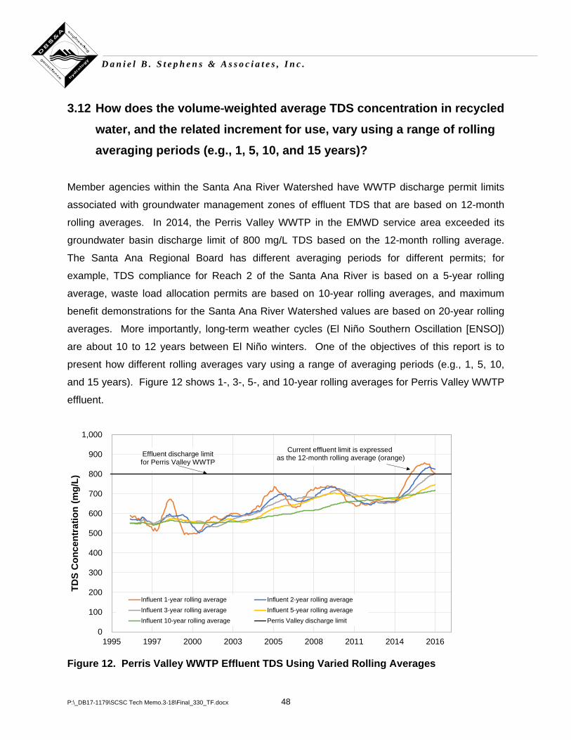
P:\_DB17-1179\SCSC Tech Memo.3-18\Final_330_TF.docx 48
D a n i e l B . S t e p h e n s & A s s o c i a t e s , I n c .
3.12 How does the volume‐weighted average TDS concentration in recycled
water, and the related increment for use, vary using a range of rolling averaging periods (e.g., 1, 5, 10, and 15 years)?
Member agencies within the Santa Ana River Watershed have WWTP discharge permit limits
associated with groundwater management zones of effluent TDS that are based on 12-month
rolling averages. In 2014, the Perris Valley WWTP in the EMWD service area exceeded its
groundwater basin discharge limit of 800 mg/L TDS based on the 12-month rolling average.
The Santa Ana Regional Board has different averaging periods for different permits; for
example, TDS compliance for Reach 2 of the Santa Ana River is based on a 5-year rolling
average, waste load allocation permits are based on 10-year rolling averages, and maximum
benefit demonstrations for the Santa Ana River Watershed values are based on 20-year rolling
averages. More importantly, long-term weather cycles (El Niño Southern Oscillation [ENSO])
are about 10 to 12 years between El Niño winters. One of the objectives of this report is to
present how different rolling averages vary using a range of averaging periods (e.g., 1, 5, 10,
and 15 years). Figure 12 shows 1-, 3-, 5-, and 10-year rolling averages for Perris Valley WWTP
effluent.
Figure 12. Perris Valley WWTP Effluent TDS Using Varied Rolling Averages
0
100
200
300
400
500
600
700
800
900
1,000
1995 1997 2000 2003 2005 2008 2011 2014 2016
TDS
Con
cent
ratio
n (m
g/L)
Influent 1-year rolling average Influent 2-year rolling averageInfluent 3-year rolling average Influent 5-year rolling averageInfluent 10-year rolling average Perris Valley discharge limit
Effluent discharge limitfor Perris Valley WWTP
Current effluent limit is expressedas the 12-month rolling average (orange)
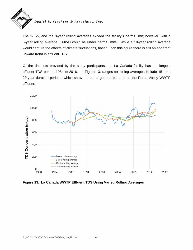
P:\_DB17-1179\SCSC Tech Memo.3-18\Final_330_TF.docx 49
D a n i e l B . S t e p h e n s & A s s o c i a t e s , I n c .
The 1-, 2-, and the 3-year rolling averages exceed the facility’s permit limit; however, with a
5-year rolling average, EMWD could be under permit limits. While a 10-year rolling average
would capture the effects of climate fluctuations, based upon this figure there is still an apparent
upward trend in effluent TDS.
Of the datasets provided by the study participants, the La Cañada facility has the longest
effluent TDS period: 1984 to 2016. In Figure 13, ranges for rolling averages include 15- and
20-year duration periods, which show the same general patterns as the Perris Valley WWTP
effluent.
Figure 13. La Cañada WWTP Effluent TDS Using Varied Rolling Averages
0
200
400
600
800
1,000
1,200
1980 1984 1989 1994 2000 2004 2009 2014 2020
TDS
Con
cent
ratio
n (m
g/L)
1-Year rolling average5-Year rolling average10-Year rolling average20-Year rolling average
P:\_DB17-1179\SCSC Tech Memo.3-18\Final_330_TF.docx 50
D a n i e l B . S t e p h e n s & A s s o c i a t e s , I n c .
4. Approaches for Evaluating TDS Trends
DBS&A employed two primary methods for modeling and evaluating long-term trends for salinity
in wastewater and recycled water. The first method is a deterministic model, where the
outcome of a deterministic/algebraic model is governed through relationships between a state
(initial conditions) and an event (parameters). WWTP influent TDS concentrations were
estimated from a measured concentration of source water and a salt load from indoor use The
second method uses statistical analyses to explore the relationship between the dependent or
response variable (WWTP influent TDS) and independent (explanatory) variables (e.g., source
concentration, population, conservation measures, etc.). Both methods are limited to the
availability of source water quality data; therefore, these analyses were performed on a subset
of the total number of sewersheds provided. At a minimum, the requisite data for the trends
analysis include the following:
• Monthly indoor water use flows – assumed to be equivalent to influent flow
• Monthly volume-weighted average TDS concentrations in source water
• Monthly TDS concentrations in influent and/or effluent flows
• Per capita salt mass load for the deterministic model (literature values)
• Population for each sewershed
4.1 Deterministic Approach to Evaluating TDS Trends
One of the key purposes of this study is to determine what effect conservation has on the quality
of water discharged by WWTPs. As an initial step in understanding this relationship, a
deterministic approach was used to model the observed influent TDS with and without
conservation measures. Influent TDS is estimated from a measured concentration of source
water and the per capita SML from indoor use multiplied by the population in the sewershed.
Salt mass in source water and salt added from indoor uses of water (human excretion, gray
water, soaps, water softeners are the two principal components of influent TDS in the
deterministic model:
Influent TDS = Source TDS + (SML*population) / (influent flow in mgd) (2)
P:\_DB17-1179\SCSC Tech Memo.3-18\Final_330_TF.docx 51
D a n i e l B . S t e p h e n s & A s s o c i a t e s , I n c .
SML is relatively constant based on the characteristics of a given sewershed and, as described
in Section 1.4, is approximately 0.15 to 0.18 pounds per capita per day. For this study, the SML
value varies by sewershed, and is determined by calibrating the starting point of the model to
the measured influent TDS. The average SML for each of the sewersheds is 0.17 pounds per
capita per day, and ranged from 0.4 pound per capita per day for OCSD to 0.04 pound per
capita per day for Padre Dam MWD. The wide variation is likely due to the industrial,
commercial, and institutional discharges into the system and underestimates or overestimates in
population or flow data provided for each sewershed.
To compare the effects of conservation, two scenarios were developed based upon influent
flow:
• Scenario 1 uses the actual influent flow values which generally declined over time
because of conservation measures.
• Scenario 2 adjusts the flow volume to represent a constant per capita indoor water use
throughout the period represented by the dataset. The constant per capita indoor water
use is assumed to be the water use at the beginning of the dataset. This scenario
shows what the influent TDS concentration would have been throughout the study period
without conservation.
The parameters used for the EMWD combined dataset for the two deterministic models
scenarios are summarized in Table 10. Figure 14 is a graphical representation of the two
scenarios for the deterministic model for the EMWD combined dataset. The black and green
lines represent the observed volume-weighted source water TDS and influent TDS,
respectively. Scenario 1 of the deterministic model is depicted as the blue dotted line and
Scenario 2 is depicted as the orange dotted line. Deterministic models for the remaining
sewersheds are provided in Appendix B. This approach is dependent on influent flow;
therefore, variations or divergences of flow can impact the model results and may artificially
overestimate the “with conservation” scenario.
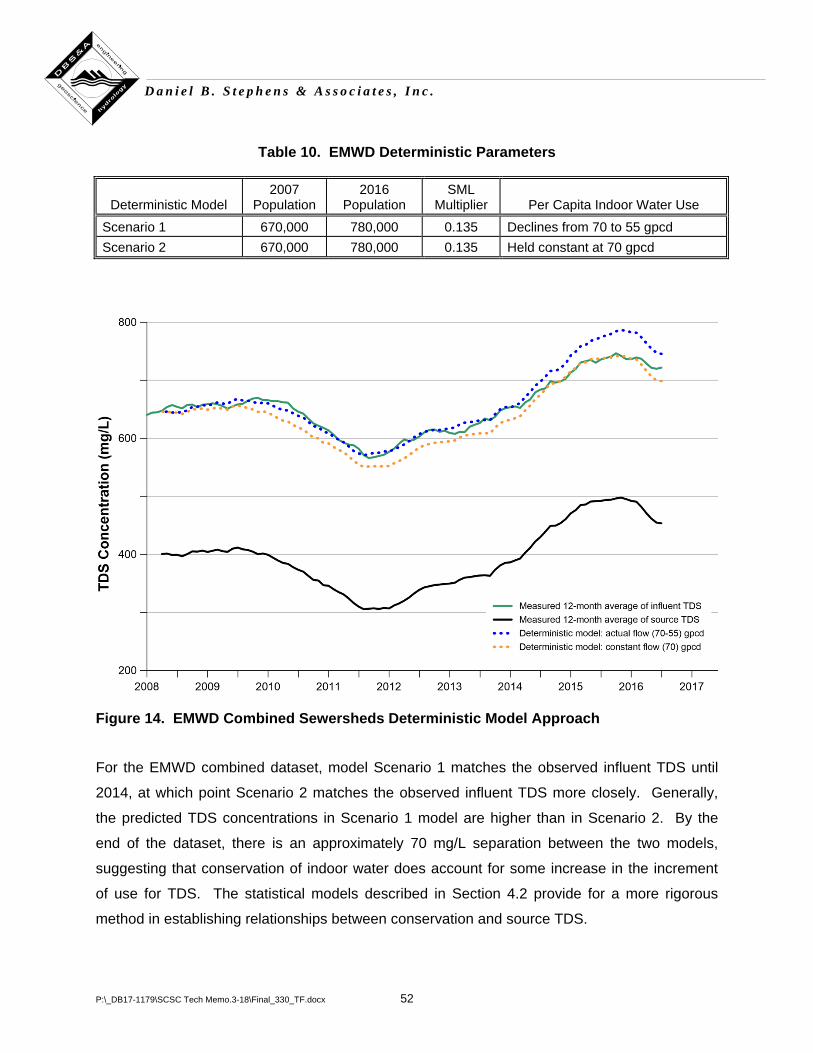
P:\_DB17-1179\SCSC Tech Memo.3-18\Final_330_TF.docx 52
D a n i e l B . S t e p h e n s & A s s o c i a t e s , I n c .
Table 10. EMWD Deterministic Parameters
Deterministic Model 2007
Population 2016
Population SML
Multiplier Per Capita Indoor Water Use
Scenario 1 670,000 780,000 0.135 Declines from 70 to 55 gpcd Scenario 2 670,000 780,000 0.135 Held constant at 70 gpcd
Figure 14. EMWD Combined Sewersheds Deterministic Model Approach
For the EMWD combined dataset, model Scenario 1 matches the observed influent TDS until
2014, at which point Scenario 2 matches the observed influent TDS more closely. Generally,
the predicted TDS concentrations in Scenario 1 model are higher than in Scenario 2. By the
end of the dataset, there is an approximately 70 mg/L separation between the two models,
suggesting that conservation of indoor water does account for some increase in the increment
of use for TDS. The statistical models described in Section 4.2 provide for a more rigorous
method in establishing relationships between conservation and source TDS.
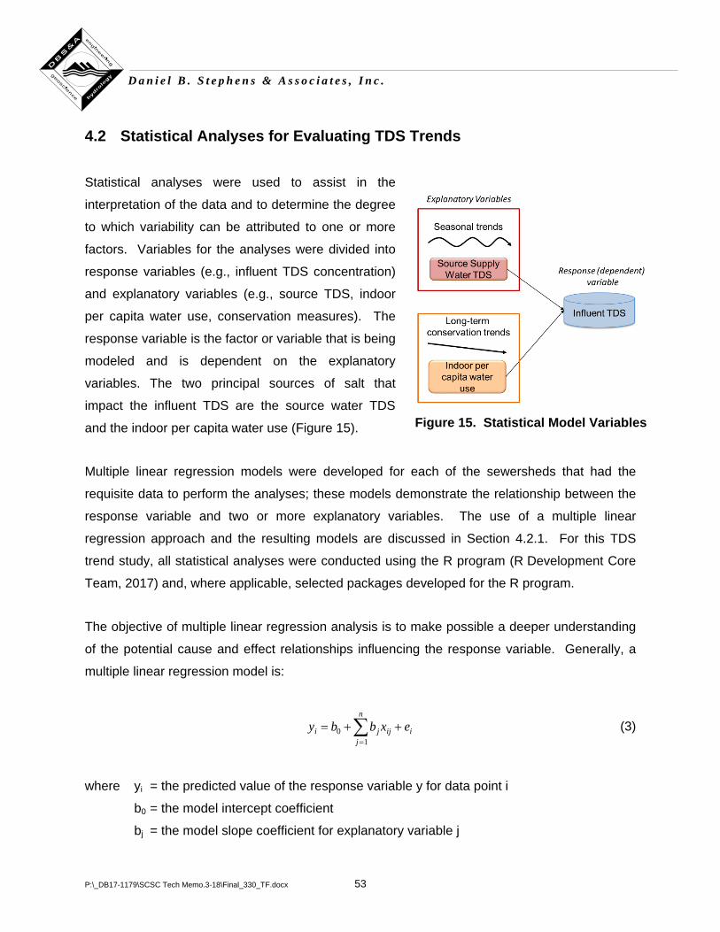
P:\_DB17-1179\SCSC Tech Memo.3-18\Final_330_TF.docx 53
D a n i e l B . S t e p h e n s & A s s o c i a t e s , I n c .
4.2 Statistical Analyses for Evaluating TDS Trends
Statistical analyses were used to assist in the
interpretation of the data and to determine the degree
to which variability can be attributed to one or more
factors. Variables for the analyses were divided into
response variables (e.g., influent TDS concentration)
and explanatory variables (e.g., source TDS, indoor
per capita water use, conservation measures). The
response variable is the factor or variable that is being
modeled and is dependent on the explanatory
variables. The two principal sources of salt that
impact the influent TDS are the source water TDS
and the indoor per capita water use (Figure 15).
Multiple linear regression models were developed for each of the sewersheds that had the
requisite data to perform the analyses; these models demonstrate the relationship between the
response variable and two or more explanatory variables. The use of a multiple linear
regression approach and the resulting models are discussed in Section 4.2.1. For this TDS
trend study, all statistical analyses were conducted using the R program (R Development Core
Team, 2017) and, where applicable, selected packages developed for the R program.
The objective of multiple linear regression analysis is to make possible a deeper understanding
of the potential cause and effect relationships influencing the response variable. Generally, a
multiple linear regression model is:
∑=
++=n
jiijji exbby
10 (3)
where yi = the predicted value of the response variable y for data point i
b0 = the model intercept coefficient
bj = the model slope coefficient for explanatory variable j
Figure 15. Statistical Model Variables
P:\_DB17-1179\SCSC Tech Memo.3-18\Final_330_TF.docx 54
D a n i e l B . S t e p h e n s & A s s o c i a t e s , I n c .
n = the total number of explanatory variables in the model
xij = the known value x of explanatory variable j for data point i
ei = the residual error of data point i from the fitted model
Multiple linear regression analysis determines the coefficients b0 and bj for a best-fit linear
model by minimizing ei, along with the statistical significance of the explanatory variables in the
model and the portion of the total variance accounted for by the model (as measured by the
multiple R2).
In addition to the basic multiple regression model (Equation 3), the R package, called “relaimpo”
(Gromping, 2015), was used to determine the relative importance of the explanatory variables in
the model. The package implements methods detailed in Gromping (2006), particularly the
‘lmg’ method, which decomposes multiple R2 values based on both direct effects and effects
adjusted for the intercorrelations of the explanatory variables in the model.
The response variable, influent TDS, was modeled as a function of the explanatory variables,
source TDS and influent flow measured in gpcd. In other words, influent TDS ~ source TDS +
influent per capita flow, where “~” denotes “is a function of.” Results are provided in Table 11.
Figure 16 is a graphical example for the EMWD combined sewershed with influent TDS as the
response variable. The black and green lines represents the observed volume-weighted source
water TDS and influent TDS, respectively. As with the deterministic model, Scenario 1 is
depicted as the blue dotted line and Scenario 2 is depicted as the orange dotted line.
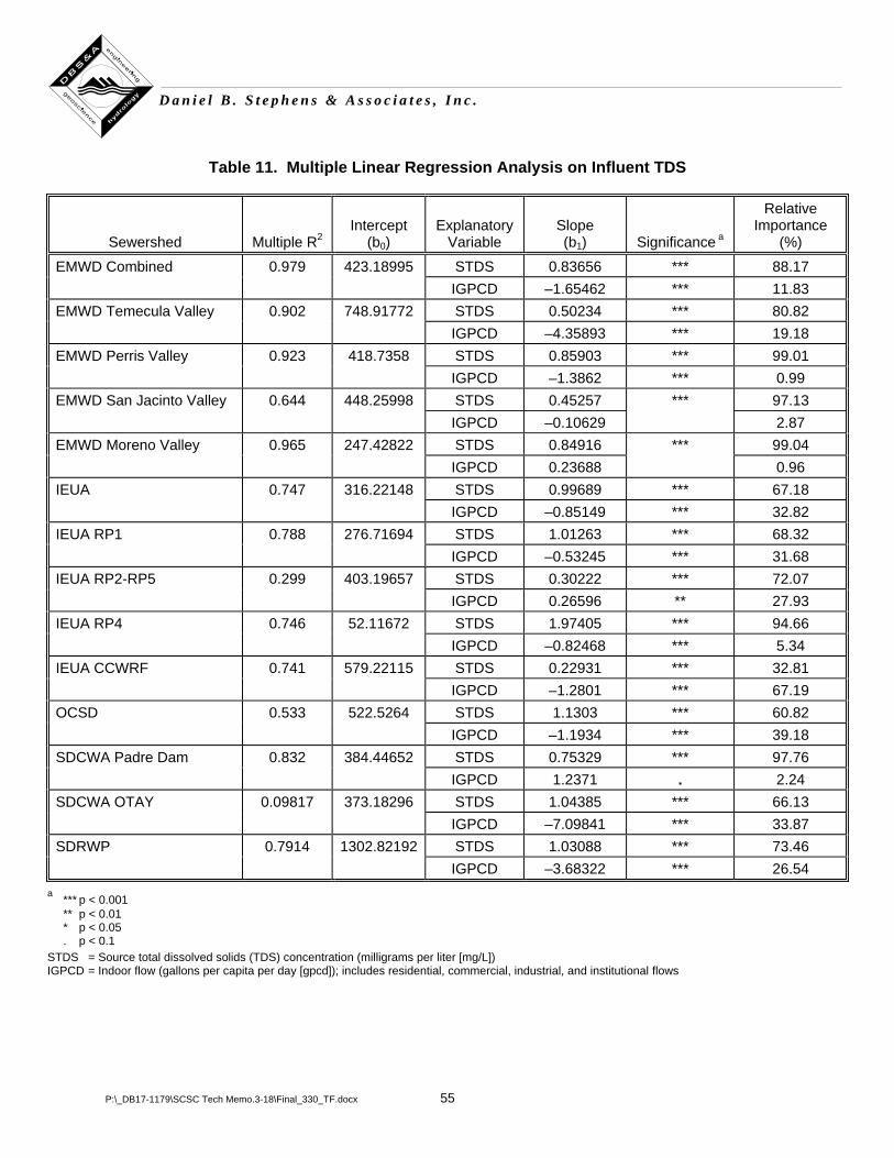
P:\_DB17-1179\SCSC Tech Memo.3-18\Final_330_TF.docx 55
D a n i e l B . S t e p h e n s & A s s o c i a t e s , I n c .
Table 11. Multiple Linear Regression Analysis on Influent TDS
Sewershed Multiple R2 Intercept
(b0) Explanatory
Variable Slope (b1) Significance a
Relative Importance
(%)
EMWD Combined 0.979 423.18995 STDS 0.83656 *** 88.17 IGPCD –1.65462 *** 11.83 EMWD Temecula Valley 0.902 748.91772 STDS 0.50234 *** 80.82 IGPCD –4.35893 *** 19.18 EMWD Perris Valley 0.923 418.7358 STDS 0.85903 *** 99.01 IGPCD –1.3862 *** 0.99 EMWD San Jacinto Valley 0.644 448.25998 STDS 0.45257 *** 97.13 IGPCD –0.10629 2.87 EMWD Moreno Valley 0.965 247.42822 STDS 0.84916 *** 99.04 IGPCD 0.23688 0.96 IEUA 0.747 316.22148 STDS 0.99689 *** 67.18 IGPCD –0.85149 *** 32.82 IEUA RP1 0.788 276.71694 STDS 1.01263 *** 68.32 IGPCD –0.53245 *** 31.68 IEUA RP2-RP5 0.299 403.19657 STDS 0.30222 *** 72.07 IGPCD 0.26596 ** 27.93 IEUA RP4 0.746 52.11672 STDS 1.97405 *** 94.66 IGPCD –0.82468 *** 5.34 IEUA CCWRF 0.741 579.22115 STDS 0.22931 *** 32.81 IGPCD –1.2801 *** 67.19 OCSD 0.533 522.5264 STDS 1.1303 *** 60.82 IGPCD –1.1934 *** 39.18 SDCWA Padre Dam 0.832 384.44652 STDS 0.75329 *** 97.76 IGPCD 1.2371 . 2.24 SDCWA OTAY 0.09817 373.18296 STDS 1.04385 *** 66.13 IGPCD –7.09841 *** 33.87 SDRWP 0.7914 1302.82192 STDS 1.03088 *** 73.46 IGPCD –3.68322 *** 26.54
a *** p < 0.001 ** p < 0.01 * p < 0.05 . p < 0.1 STDS = Source total dissolved solids (TDS) concentration (milligrams per liter [mg/L]) IGPCD = Indoor flow (gallons per capita per day [gpcd]); includes residential, commercial, industrial, and institutional flows
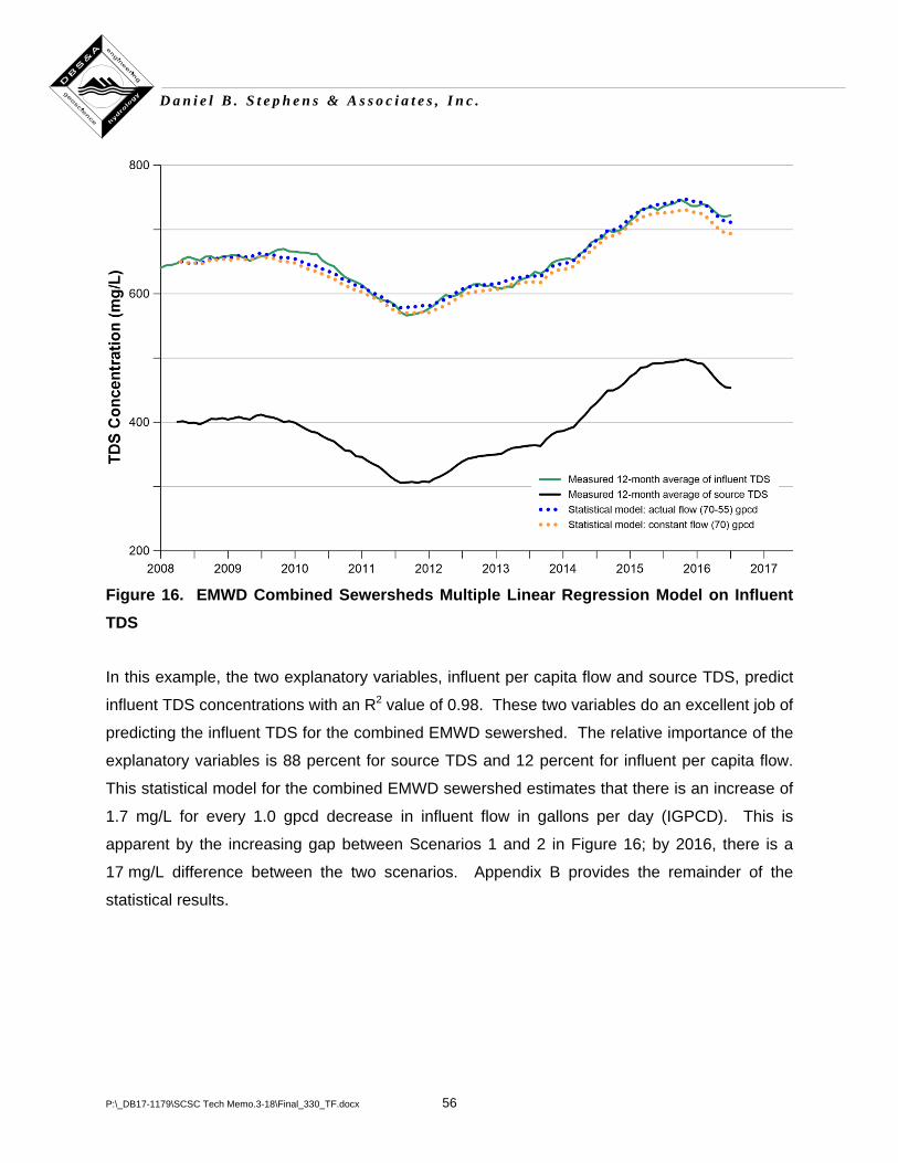
P:\_DB17-1179\SCSC Tech Memo.3-18\Final_330_TF.docx 56
D a n i e l B . S t e p h e n s & A s s o c i a t e s , I n c .
Figure 16. EMWD Combined Sewersheds Multiple Linear Regression Model on Influent TDS
In this example, the two explanatory variables, influent per capita flow and source TDS, predict
influent TDS concentrations with an R2 value of 0.98. These two variables do an excellent job of
predicting the influent TDS for the combined EMWD sewershed. The relative importance of the
explanatory variables is 88 percent for source TDS and 12 percent for influent per capita flow.
This statistical model for the combined EMWD sewershed estimates that there is an increase of
1.7 mg/L for every 1.0 gpcd decrease in influent flow in gallons per day (IGPCD). This is
apparent by the increasing gap between Scenarios 1 and 2 in Figure 16; by 2016, there is a
17 mg/L difference between the two scenarios. Appendix B provides the remainder of the
statistical results.
P:\_DB17-1179\SCSC Tech Memo.3-18\Final_330_TF.docx 57
D a n i e l B . S t e p h e n s & A s s o c i a t e s , I n c .
5. Summary
A majority of WWTPs in this study exhibited an increase in influent and effluent TDS
concentrations over the past few decades. This study found that the two primary contributors to
increasing TDS in WWTPs are (1) volume-weighted source water quality and (2) decreased
indoor water use. Source water quality is a function of temporal trends as a consequence of
drought cycles and long-term climate change, among other factors. The decreased availability
of reliable, high-quality potable water supplies may result in water supply agencies changing
their water supply options and augmenting their portfolio to include lower quality sources,
including switching from SWP water to CRA water or groundwater that may have higher TDS.
Drought and climate change impact water quality directly and secondarily by changing the
source of the water. Water conservation measures—in part due to recent historic drought
cycles—has resulted in decreased indoor water use and a corresponding increase in TDS. This
is an unintended and largely unanticipated consequence of well-intentioned water conservation
measures. The salt mass added through an increment of use for indoor water uses remains
about the same, while the volume of water decreases, resulting in increased TDS
concentrations.
The key findings of this study include:
• Volume-weighted source water TDS concentration is the significant determiner of
influent TDS. Source TDS explains more of the variability in influent/effluent TDS than
any other factor, including decreased indoor water use.
• There is a strong inverse correlation between drought and imported water TDS
concentrations for both SWP water and CRA water. TDS concentration can vary by
300 mg/L from wet years to dry years for CRA water and by 200 mg/L for SWP water.
• Long-term conservation efforts account for a smaller, but still significant, increase in
TDS. IEUA and EMWD statistical models predict a 1.2 to 1.7 mg/L increase in TDS for
every 1.0 gpcd decrease in indoor water use.
P:\_DB17-1179\SCSC Tech Memo.3-18\Final_330_TF.docx 58
D a n i e l B . S t e p h e n s & A s s o c i a t e s , I n c .
• Other unintended consequences of water conservation measures include loss of
revenue from water sales, less available recycled water, and increased infrastructure
operation and maintenance costs. Unintended benefits include a reduction in energy
costs and decreased greenhouse gas formation.
• The reduction in the number of SRWS units can significantly reduce the concentration of
TDS in influent flows to the WWTPs. In a case study, SCVSD removed 8,000 SRWS
units, thereby reducing the TDS in the WWTP influent flow by nearly 80 mg/L.
• The duration of rolling-average periods can determine whether or not an agency is in
violation of their permit limits. A compliance limit based on a 5-year rolling average
instead of a 1-year rolling average for the Perris Valley WWTP would have kept the
WWTP within permit limits.
P:\_DB17-1179\SCSC Tech Memo.3-18\Final_330_TF.docx 59
D a n i e l B . S t e p h e n s & A s s o c i a t e s , I n c .
References
Aparicio, A., E. Rodriguez-Rodriguez, E. Cuadrado-Soto, B. Navia, A.M. López-Sobaler, and
R.M. Ortega. 2017. Estimation of salt intake assessed by urinary excretion of sodium over
24 h in Spanish subjects aged 7–11 years. European Journal of Nutrition 56(1):171-178.
Bookman Edmonston Engineering. 1997. Salinity management study, Phase 1, Progress report.
Prepared for the Metropolitan Water District of Southern California and the U.S. Bureau of
Reclamation. February 1997.
California Department of Finance. 2012. E-4 population estimates for cities, counties, and the
state, 2001-2010, with 2000 & 2010 census counts. November 2012.
California Department of Finance. 2016. E-2 California county population estimates and
components of change by year, July 1, 2010-2016. December 2016.
California Department of Finance. 2017 Online population estimates. Accessed at
<http://www.dof.ca.gov/Forecasting/Demographics/Estimates/>.
California Executive Department (CED). 2014a. Emergency Proclamation. January 17, 2014.
CED. 2014b. Emergency Proclamation. April 25, 2014.
CED 2014c. Executive Order B-28-14. December 22, 2014.
CED 2015. Executive Order B-29-15. April 1, 2015.
CED 2016. Executive Order B-37-16. May 9, 2016.
CED 2017a. Updated to the Water Code (Assemble Bill 968 Section 10608.25). February 16,
2017.
P:\_DB17-1179\SCSC Tech Memo.3-18\Final_330_TF.docx 60
D a n i e l B . S t e p h e n s & A s s o c i a t e s , I n c .
CED 2017b. Executive Order B-40-17. April 7, 2017.
California Natural Resources Agency, California Department of Food & Agriculture, and the
California Environmental Protection Agency (State of California). 2016. California water
action plan - 2016 update.
California Urban Water Agencies (CUWA). 2017. Adapting to change: Utility systems and
declining flows. In partnership with the California Association of Sanitation Agencies, Water
Research Foundation, WateReuse California, and the California Water Environment
Association. November 2017.
DeOreo, W.B., P.W. Mayer, L. Martien, M. Hayden, A. Funk, M. Kramer-Duffield, and R. Davis.
2017. California single-family water use efficiency study. California Department of Water
Resources. September 30, 2012 (Revised September 27, 2017).
Department of Water Resources, State of California (DWR). 1994. California water plan update.
DWR Bulletin 160-93. October 1994.
DWR. 2009. Water Conservation Act of 2009 (Senate Bill X7-7). Available at
<https://www.water.ca.gov/Programs/Water-Use-And-Efficiency/SB-X7-7>. November 10,
2009.
DWR. 2013. California water plan, Update 2013: Investing in innovation & infrastructure.
DWR. 2018. North Sierra Precipitation: 8-Station Index. California Data Exchange Center.
<http://cdec.water.ca.gov/precipapp/get8SIPrecipIndex.action. Accessed February 2018>.
Gleick, P., D. Haasz, C. Henges-Jeck, V. Srinivasan, G. Wolff, K. Kao Cushing, and A. Mann.
2003. Waste not, want not: The potential for urban water conservation in California. Pacific
Institute. November 2003.
Gromping, U. 2006. Relative importance for linear regression in R: The package relaimpo.
Journal of Statistical Software 17(1).
P:\_DB17-1179\SCSC Tech Memo.3-18\Final_330_TF.docx 61
D a n i e l B . S t e p h e n s & A s s o c i a t e s , I n c .
Gromping, U. 2015. relaimpo: Relative importance of regressors in linear models. R package
version 2.2-2. <https://cran.r-project.org/web/packages/relaimpo/index.html>.
Heberger, M., H. Cooley, and P. Gleick. 2014. Urban water conservation and efficiency potential
in California. Pacific Institute/Natural Resources Defense Council. June 2014.
Inland Empire Utilities Agency (IEUA). 2012. Residential Self-Regenerating Water Softener
Removal Rebate Program, Final report. June 2012.
Jessen. 2015. The impact of self-regenerating water softeners on water management. 2015
Multi-State Salinity Coalition Annual Salinity Summit. February 20, 2015.
Los Angeles County Sanitation Districts (LACSD). 2002. Santa Clarita Valley Joint Sewerage
System, Chloride source report. October 2002.
LACSD. 2014. Chloride source identification/reduction, pollution prevention, and public outreach
plan. November 2014.
LACSD. 2017. Automatic water softeners in the Santa Clarita Valley. Accessed October 2017 at
<http://www.lacsd.org/wastewater/automatic_water_softeners/default.asp>.
Mayer, P.W., W.B. DeOreo, E.M. Opitz, J.C. Kiefer, W.Y. Davis, B. Dziegielewski, and J.O.
Nelson. 1999. Residential end uses of water, Final Report. AWWA Research Foundation.
Metropolitan Water District of Southern California (MWDSC). 2016. 2015 Urban water
management plan. June 2016.
Mount, J. and E. Hanak. 2016. Water use in California. Public Policy Institute of California. July
2016.
Nall, D.H. and R. Sedak. 2013. Total dissolved solids in reclaimed water. American Society of
Heating, Refrigerating and Air-Conditioning Engineers (ASHRAE) Journal (October).
P:\_DB17-1179\SCSC Tech Memo.3-18\Final_330_TF.docx 62
D a n i e l B . S t e p h e n s & A s s o c i a t e s , I n c .
National Oceanic and Atmospheric Administration (NOAA). 2017. Palmer Drought Severity
Index. <https://climatedataguide.ucar.edu/climate-data/palmer-drought-severity-index-pdsi>.
Accessed August 2017.
Public Policy Institute of California (PPIC). 2017. Just the facts: California’s population.
<http://www.ppic.org/publication/californias-population/>.
R Development Core Team. 2017. R: A language and environment for statistical computing. R
Foundation for Statistical Computing, Vienna, Austria.
Regional Water Quality Control Board (RWQCB). 2015. About recycling.
<http://www.water.ca.gov/recycling>. Accessed September 2017.
Ripley, B. 2016. tree: Classification and regression trees. R package version 1.0-37.
<https://cran.r-project.org/web/packages/tree/tree.pdf>.
Revelle, W. 2017. psych: Procedures for psychological, psychometric, and personality research.
R package version 1.7.8. <https://cran.r-project.org/web/packages/psych/psych.pdf>.
San Diego County Water Authority (SDCWA). 2017. Dataset provided by SDCWA for the SCSC
TDS trend study.
Santa Ana Watershed Project Authority (SAWPA). 2018. Inland Empire Brine Line.
<http://www.sawpa.org/wp-content/uploads/2015/08/SAWPA_Brine-Line_Brochure.pdf>
Accessed February 2018.
Southern California Salinity Coalition (SCSC). 2009. Salinity and water softeners.
<http://www.socalsalinity.org/pdfs/SCSCFactSheetonSalinityandWaterSoftenersAugust2009
.pdf>
SCSC. 2017. About SCSC. <www.socalsalinity.org>.
P:\_DB17-1179\SCSC Tech Memo.3-18\Final_330_TF.docx 63
D a n i e l B . S t e p h e n s & A s s o c i a t e s , I n c .
Spang, E.S., A.J. Holguin, and F.J. Loge. 2018. The estimated impact of California’s urban
water conservation mandate on electricity consumption and greenhouse gas emissions.
Environmental Research Letters (January).
State Water Resources Control Board (SWRCB). 2009. Recycled Water Policy.
<https://www.waterboards.ca.gov/water_issues/programs/water_recycling_policy/docs/recyc
ledwaterpolicy_approved.pdf>.
SWRCB. 2013. Policy for Water Quality Control for Recycled Water (Recycled Water Policy).
<https://www.waterboards.ca.gov/water_issues/programs/water_recycling_policy/docs/rwp_r
evtoc.pdf>.
SWRCB. 2017. Resolution No. 2017-0012. Comprehensive Response to Climate Change.
<https://www.waterboards.ca.gov/board_decisions/adopted_orders/resolutions/2017/rs2017
_0012.pdf>.
Thompson, K., W. Christofferson, D. Robinette, J. Curl, L. Baker, J. Brereton, and K. Reich.
2006. Characterizing and managing salinity loadings in reclaimed water systems. Jointly
sponsored and published by AWWA Research Foundation and WateReuse Foundation.
Tran, Q.K., D. Jassby, and K.A. Schwabe. 2017. The implications of drought and water
conservation on the reuse of municipal wastewater: Recognizing impacts and identifying
mitigation possibilities. Journal of Water Research. Available at
<http://www.sciencedirect.com/science/article/pii/S004313541730814X>.
U.S. Department of the Interior (U.S. DOI). 2017. Colorado River Basin Water Agreements.
<https://www.doi.gov/pressreleases/secretary-jewell-directs-continued-work-crucial-
colorado-river-basin-water-0>.
U.S. Environmental Protection Agency (U.S. EPA). 1980. Effects of water conservation induced
wastewater flow reduction: A perspective. EPA-600/2-80-137. August 1980.
P:\_DB17-1179\SCSC Tech Memo.3-18\Final_330_TF.docx 64
D a n i e l B . S t e p h e n s & A s s o c i a t e s , I n c .
U.S. EPA. 2005. Combined retrofit report: Water and energy savings from high efficiency
fixtures and appliances in single family homes. Volume 1. March 28, 2005.
U.S. EPA. 2018. Bay Delta Conservation Plan / California WaterFix. Available at
<https://www.epa.gov/sfbay-delta/bay-delta-conservation-plan-california-waterfix>.
U.S. Geological Survey (USGS). 2016a. Water hardness and alkalinity. Accessed at
<https://water.usgs.gov/owq/hardness-alkalinity.html>. December 28, 2016.
USGS. 2016b. Water hardness. <https://water.usgs.gov/owq/hardness-alkalinity.html>.
December 15, 2016.
World Health Organization (WHO). 2016. Fact sheet: Salt reduction. Reviewed June 2016.
<http://www.who.int/mediacentre/factsheets/fs393/en/>.
Appendix A
Influent and Effluent TDS Trends
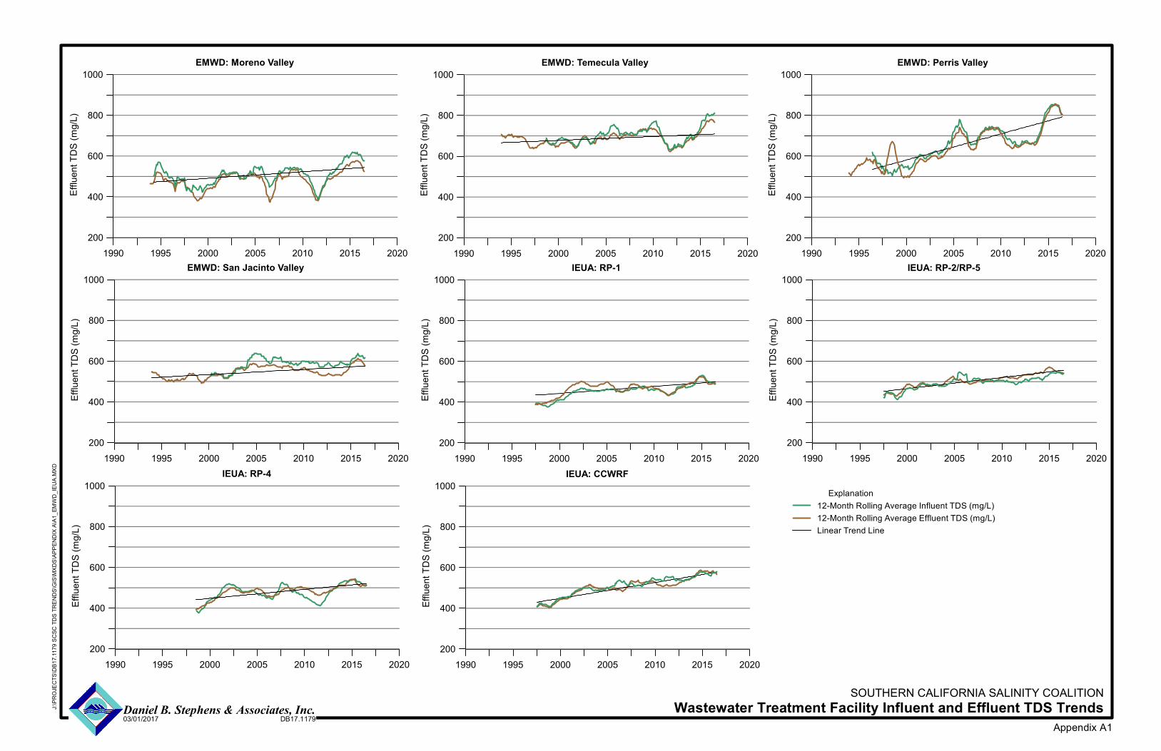
Appendix A1
SOUTHERN CALIFORNIA SALINITY COALITIONWastewater Treatment Facility Influent and Effluent TDS TrendsDaniel B. Stephens & Associates, Inc.
03/01/2017 DB17.1179
J:\PR
OJEC
TS\D
B17.1
179 S
CSC
TDS T
REND
S\GIS\
MXDS
\APPE
NDIX
A\A1_
EMWD
_IEUA
.MXD
1990 1995 2000 2005 2010 2015 2020200
400
600
800
1000EMWD: Moreno Valley
Efflue
nt TD
S (mg
/L)
1990 1995 2000 2005 2010 2015 2020200
400
600
800
1000EMWD: Temecula Valley
Efflue
nt TD
S (mg
/L)
1990 1995 2000 2005 2010 2015 2020200
400
600
800
1000EMWD: Perris Valley
Efflue
nt TD
S (mg
/L)
1990 1995 2000 2005 2010 2015 2020200
400
600
800
1000EMWD: San Jacinto Valley
Efflue
nt TD
S (mg
/L)
1990 1995 2000 2005 2010 2015 2020200
400
600
800
1000
Explanation12-Month Rolling Average Influent TDS (mg/L)12-Month Rolling Average Effluent TDS (mg/L)Linear Trend Line
IEUA: RP-1
Efflue
nt TD
S (mg
/L)
1990 1995 2000 2005 2010 2015 2020200
400
600
800
1000IEUA: RP-2/RP-5
Efflue
nt TD
S (mg
/L)
1990 1995 2000 2005 2010 2015 2020200
400
600
800
1000IEUA: RP-4
Efflue
nt TD
S (mg
/L)
1990 1995 2000 2005 2010 2015 2020200
400
600
800
1000IEUA: CCWRF
Efflue
nt TD
S (mg
/L)
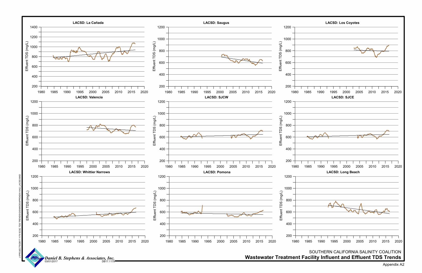
Appendix A2
SOUTHERN CALIFORNIA SALINITY COALITIONWastewater Treatment Facility Influent and Effluent TDS TrendsDaniel B. Stephens & Associates, Inc.
03/01/2017 DB17.1179
J:\PR
OJEC
TS\D
B17.1
179 S
CSC
TDS T
REND
S\GIS\
MXDS
\APPE
NDIX
A\A2_
LACS
D.MX
D
1980 1985 1990 1995 2000 2005 2010 2015 2020200
400
600
800
1000
1200
1400LACSD: La Cañada
Efflue
nt TD
S (mg
/L)
1980 1985 1990 1995 2000 2005 2010 2015 2020200
400
600
800
1000
1200LACSD: Saugus
Efflue
nt TD
S (mg
/L)
1980 1985 1990 1995 2000 2005 2010 2015 2020200
400
600
800
1000
1200LACSD: Los Coyotes
Efflue
nt TD
S (mg
/L)
1980 1985 1990 1995 2000 2005 2010 2015 2020200
400
600
800
1000
1200LACSD: Valencia
Efflue
nt TD
S (mg
/L)
1980 1985 1990 1995 2000 2005 2010 2015 2020200
400
600
800
1000
1200LACSD: SJCW
Efflue
nt TD
S (mg
/L)
1980 1985 1990 1995 2000 2005 2010 2015 2020200
400
600
800
1000
1200LACSD: SJCE
Efflue
nt TD
S (mg
/L)
1980 1985 1990 1995 2000 2005 2010 2015 2020200
400
600
800
1000
1200LACSD: Whittier Narrows
Efflue
nt TD
S (mg
/L)
1980 1985 1990 1995 2000 2005 2010 2015 2020200
400
600
800
1000
1200LACSD: Pomona
Efflue
nt TD
S (mg
/L)
1980 1985 1990 1995 2000 2005 2010 2015 2020200
400
600
800
1000
1200LACSD: Long Beach
Efflue
nt TD
S (mg
/L)
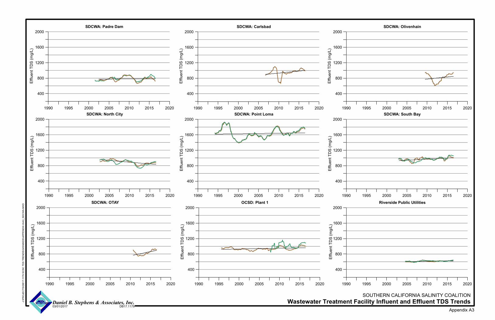
Appendix A3
SOUTHERN CALIFORNIA SALINITY COALITIONWastewater Treatment Facility Influent and Effluent TDS TrendsDaniel B. Stephens & Associates, Inc.
03/01/2017 DB17.1179
J:\PR
OJEC
TS\D
B17.1
179 S
CSC
TDS T
REND
S\GIS\
MXDS
\APPE
NDIX
A\A3_
SDCW
A.MXD
1990 1995 2000 2005 2010 2015 2020
400
800
1200
1600
2000SDCWA: Padre Dam
Efflue
nt TD
S (mg
/L)
1990 1995 2000 2005 2010 2015 2020
400
800
1200
1600
2000SDCWA: Carlsbad
Efflue
nt TD
S (mg
/L)
1990 1995 2000 2005 2010 2015 2020
400
800
1200
1600
2000SDCWA: Olivenhain
Efflue
nt TD
S (mg
/L)
1990 1995 2000 2005 2010 2015 2020
400
800
1200
1600
2000SDCWA: North City
Efflue
nt TD
S (mg
/L)
Efflue
nt TD
S (mg
/L)
Efflue
nt TD
S (mg
/L)
1990 1995 2000 2005 2010 2015 2020
400
800
1200
1600
2000SDCWA: Point Loma
1990 1995 2000 2005 2010 2015 2020
400
800
1200
1600
2000SDCWA: OTAY
1990 1995 2000 2005 2010 2015 2020
400
800
1200
1600
2000OCSD: Plant 1
Efflue
nt TD
S (mg
/L)
Efflue
nt TD
S (mg
/L)
Efflue
nt TD
S (mg
/L)
1990 1995 2000 2005 2010 2015 2020
400
800
1200
1600
2000SDCWA: South Bay
1990 1995 2000 2005 2010 2015 2020
400
800
1200
1600
2000Riverside Public Utilities
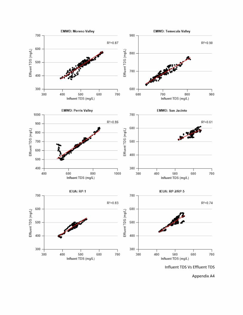
Influent TDS Vs Effluent TDS
Appendix A4
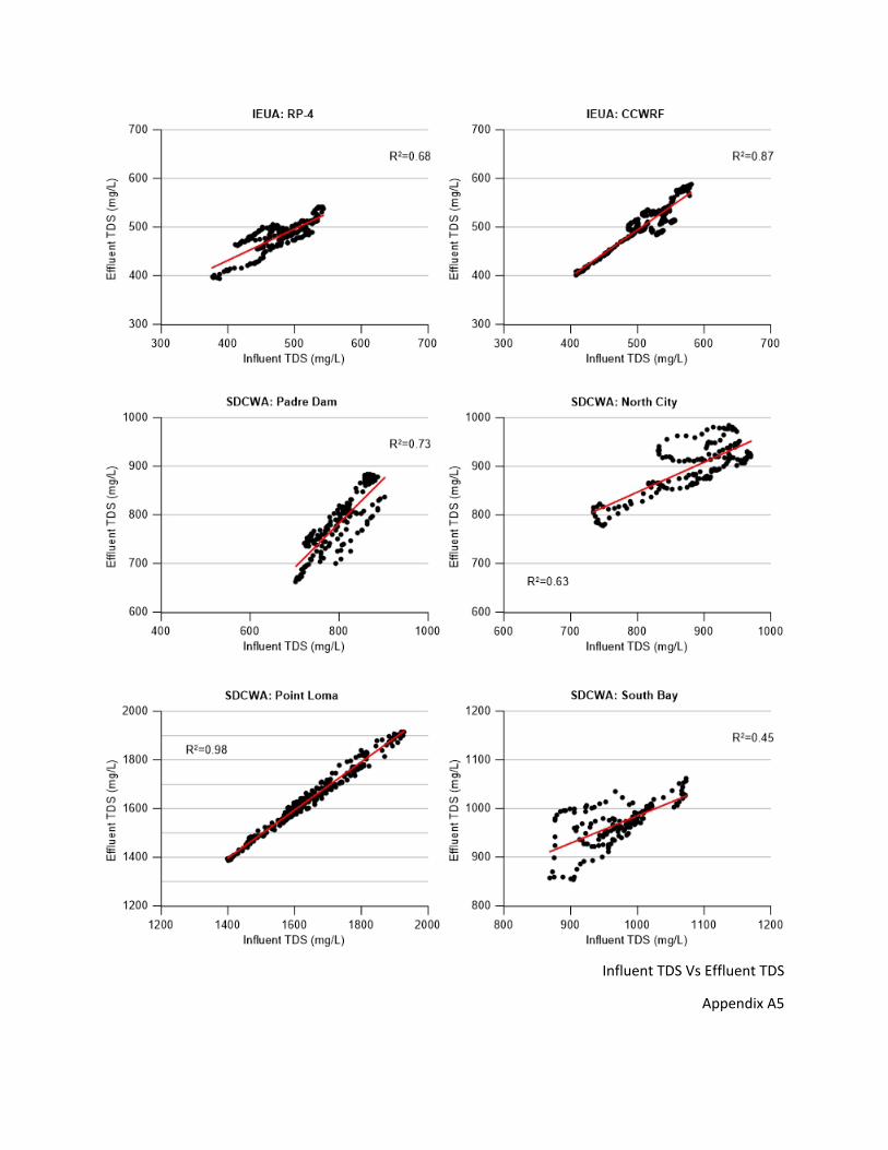
Influent TDS Vs Effluent TDS
Appendix A5
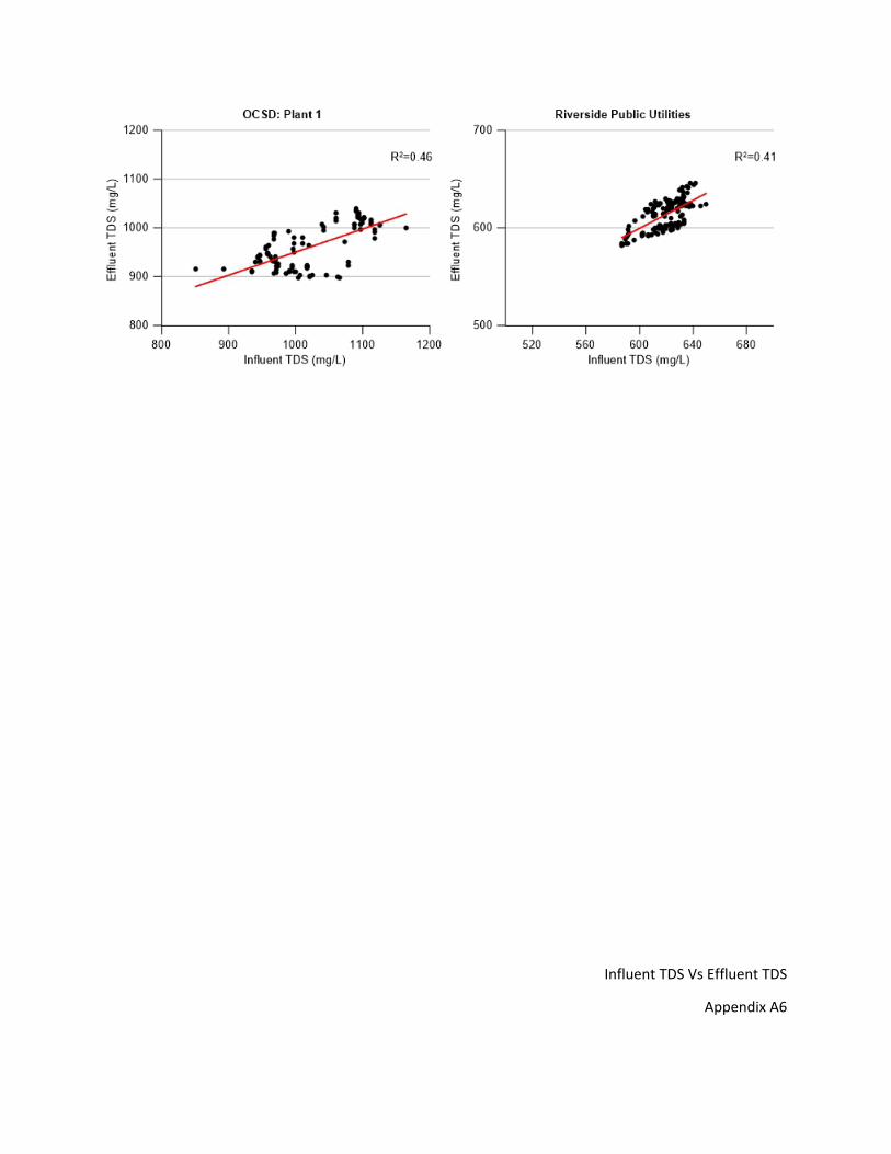
Influent TDS Vs Effluent TDS
Appendix A6
Appendix B
Indoor Water Use, TDS Trends, and
Deterministic and Statistical Model Results
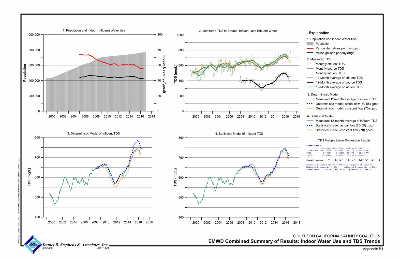
2000 2002 2004 2006 2008 2010 2012 2014 2016 20180
200,000
400,000
600,000
800,000
1,000,000
0
20
40
60
80
1001. Population and Indoor Water Use
PopulationPer capita gallons per day (gpcd)Million gallons per day (mgd)
1. Population and Indoor (Influent) Water Use
2000 2002 2004 2006 2008 2010 2012 2014 2016 20180
200
400
600
800
1000
2. Measured TDSMonthly effluent TDSMonthly source TDSMonthly influent TDS12-Month average of effluent TDS12-Month average of source TDS12-Month average of influent TDS
2. Measured TDS in Source, Influent, and Effluent WaterPo
pulat
ion
Indoor Use (mgd/gpcd)
TDS (
mg/L)
2000 2002 2004 2006 2008 2010 2012 2014 2016 2018400
500
600
700
800
3. Deterministic ModelMeasured 12-month average of influent TDSDeterministic model: actual flow (70-55) gpcdDeterministic model: constant flow (70) gpcd
3. Deterministic Model of Influent TDS
2000 2002 2004 2006 2008 2010 2012 2014 2016 2018400
500
600
700
800
4. Statistical ModelMeasured 12-month average of influent TDSStatistical model: actual flow (70-55) gpcdStatistical model: constant flow (70) gpcd
4. Statistical Model of Influent TDS
TDS (
mg/L)
TDS (
mg/L)
Explanation
Appendix B1
SOUTHERN CALIFORNIA SALINITY COALITIONEMWD Combined Summary of Results: Indoor Water Use and TDS TrendsDaniel B. Stephens & Associates, Inc.
3/22/2018 DB17.1179
J:\PR
OJEC
TS\D
B17.1
179 S
CSC
TDS T
REND
S\GIS\
MXDS
\APPE
NDIX
B\B1 E
MWD
COMB
O.MX
D
ITDS Multiple Linear Regression Results
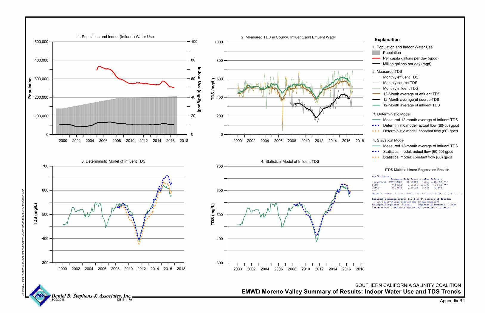
2000 2002 2004 2006 2008 2010 2012 2014 2016 20180
100,000
200,000
300,000
400,000
500,000
0
20
40
60
80
1001. Population and Indoor Water Use
PopulationPer capita gallons per day (gpcd)Million gallons per day (mgd)
1. Population and Indoor (Influent) Water Use
2000 2002 2004 2006 2008 2010 2012 2014 2016 20180
200
400
600
800
1000
2. Measured TDSMonthly effluent TDSMonthly source TDSMonthly influent TDS12-Month average of effluent TDS12-Month average of source TDS12-Month average of influent TDS
2. Measured TDS in Source, Influent, and Effluent WaterPo
pulat
ion
Indoor Use (mgd/gpcd)
TDS (
mg/L)
2000 2002 2004 2006 2008 2010 2012 2014 2016 2018300
400
500
600
700
3. Deterministic ModelMeasured 12-month average of influent TDSDeterministic model: actual flow (60-50) gpcdDeterministic model: constant flow (60) gpcd
3. Deterministic Model of Influent TDS
2000 2002 2004 2006 2008 2010 2012 2014 2016 2018300
400
500
600
700
4. Statistical ModelMeasured 12-month average of influent TDSStatistical model: actual flow (60-50) gpcdStatistical model: constant flow (60) gpcd
4. Statistical Model of Influent TDS
TDS (
mg/L)
TDS (
mg/L)
Explanation
Appendix B2
SOUTHERN CALIFORNIA SALINITY COALITIONEMWD Moreno Valley Summary of Results: Indoor Water Use and TDS TrendsDaniel B. Stephens & Associates, Inc.
3/22/2018 DB17.1179
J:\PR
OJEC
TS\D
B17.1
179 S
CSC
TDS T
REND
S\GIS\
MXDS
\APPE
NDIX
B\B2 E
MWD
MORE
NO.M
XD
ITDS Multiple Linear Regression Results
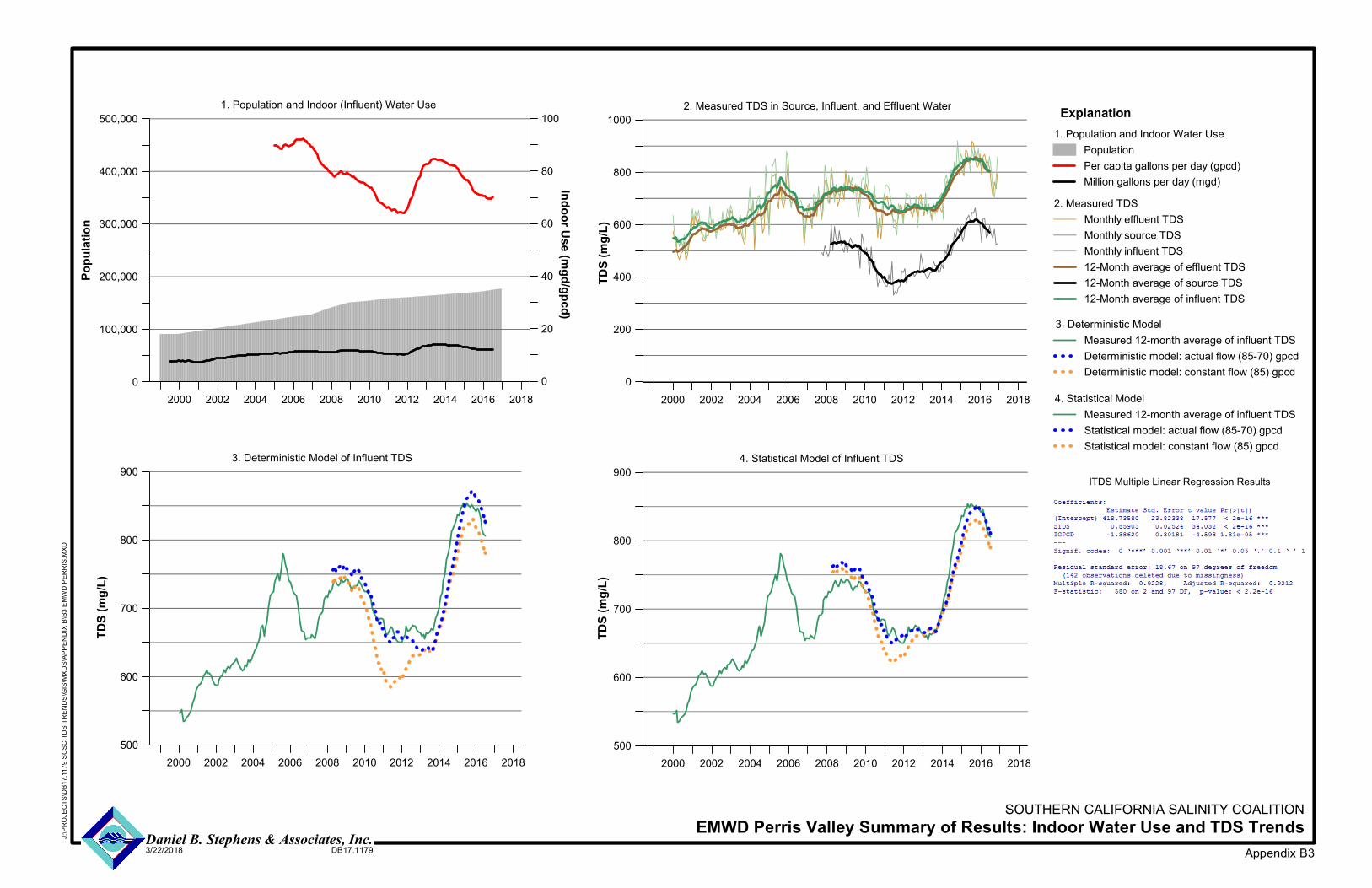
2000 2002 2004 2006 2008 2010 2012 2014 2016 20180
100,000
200,000
300,000
400,000
500,000
0
20
40
60
80
1001. Population and Indoor Water Use
PopulationPer capita gallons per day (gpcd)Million gallons per day (mgd)
1. Population and Indoor (Influent) Water Use
2000 2002 2004 2006 2008 2010 2012 2014 2016 20180
200
400
600
800
1000
2. Measured TDSMonthly effluent TDSMonthly source TDSMonthly influent TDS12-Month average of effluent TDS12-Month average of source TDS12-Month average of influent TDS
2. Measured TDS in Source, Influent, and Effluent WaterPo
pulat
ion
Indoor Use (mgd/gpcd)
TDS (
mg/L)
2000 2002 2004 2006 2008 2010 2012 2014 2016 2018500
600
700
800
900
3. Deterministic ModelMeasured 12-month average of influent TDSDeterministic model: actual flow (85-70) gpcdDeterministic model: constant flow (85) gpcd
3. Deterministic Model of Influent TDS
2000 2002 2004 2006 2008 2010 2012 2014 2016 2018500
600
700
800
900
4. Statistical ModelMeasured 12-month average of influent TDSStatistical model: actual flow (85-70) gpcdStatistical model: constant flow (85) gpcd
4. Statistical Model of Influent TDS
TDS (
mg/L)
TDS (
mg/L)
Explanation
Appendix B3
SOUTHERN CALIFORNIA SALINITY COALITIONEMWD Perris Valley Summary of Results: Indoor Water Use and TDS TrendsDaniel B. Stephens & Associates, Inc.
3/22/2018 DB17.1179
J:\PR
OJEC
TS\D
B17.1
179 S
CSC
TDS T
REND
S\GIS\
MXDS
\APPE
NDIX
B\B3 E
MWD
PERR
IS.MX
D
ITDS Multiple Linear Regression Results
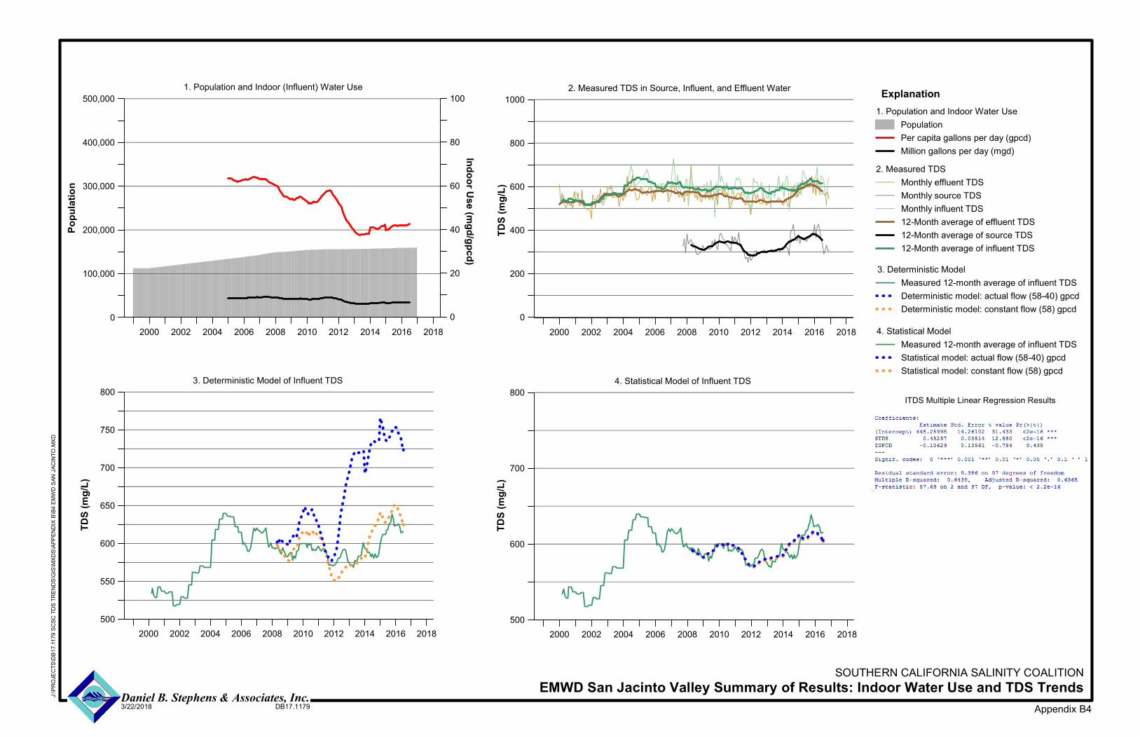
2000 2002 2004 2006 2008 2010 2012 2014 2016 20180
100,000
200,000
300,000
400,000
500,000
0
20
40
60
80
1001. Population and Indoor Water Use
PopulationPer capita gallons per day (gpcd)Million gallons per day (mgd)
1. Population and Indoor (Influent) Water Use
2000 2002 2004 2006 2008 2010 2012 2014 2016 20180
200
400
600
800
1000
2. Measured TDSMonthly effluent TDSMonthly source TDSMonthly influent TDS12-Month average of effluent TDS12-Month average of source TDS12-Month average of influent TDS
2. Measured TDS in Source, Influent, and Effluent WaterPo
pulat
ion
Indoor Use (mgd/gpcd)
TDS (
mg/L)
2000 2002 2004 2006 2008 2010 2012 2014 2016 2018500
550
600
650
700
750
800
3. Deterministic ModelMeasured 12-month average of influent TDSDeterministic model: actual flow (58-40) gpcdDeterministic model: constant flow (58) gpcd
3. Deterministic Model of Influent TDS
2000 2002 2004 2006 2008 2010 2012 2014 2016 2018500
600
700
800
4. Statistical ModelMeasured 12-month average of influent TDSStatistical model: actual flow (58-40) gpcdStatistical model: constant flow (58) gpcd
4. Statistical Model of Influent TDS
TDS (
mg/L)
TDS (
mg/L)
Explanation
Appendix B4
SOUTHERN CALIFORNIA SALINITY COALITIONEMWD San Jacinto Valley Summary of Results: Indoor Water Use and TDS TrendsDaniel B. Stephens & Associates, Inc.
3/22/2018 DB17.1179
J:\PR
OJEC
TS\D
B17.1
179 S
CSC
TDS T
REND
S\GIS\
MXDS
\APPE
NDIX
B\B4 E
MWD
SAN
JACI
NTO.
MXD
ITDS Multiple Linear Regression Results

2000 2002 2004 2006 2008 2010 2012 2014 2016 20180
100,000
200,000
300,000
400,000
500,000
0
20
40
60
80
1001. Population and Indoor Water Use
PopulationPer capita gallons per day (gpcd)Million gallons per day (mgd)
1. Population and Indoor (Influent) Water Use
2000 2002 2004 2006 2008 2010 2012 2014 2016 20180
200
400
600
800
1000
2. Measured TDSMonthly effluent TDSMonthly source TDSMonthly influent TDS12-Month average of effluent TDS12-Month average of source TDS12-Month average of influent TDS
2. Measured TDS in Source, Influent, and Effluent WaterPo
pulat
ion
Indoor Use (mgd/gpcd)
TDS (
mg/L)
2000 2002 2004 2006 2008 2010 2012 2014 2016 2018500
550
600
650
700
750
800
3. Deterministic ModelMeasured 12-month average of influent TDSDeterministic model: actual flow (58-40) gpcdDeterministic model: constant flow (58) gpcd
3. Deterministic Model of Influent TDS
2000 2002 2004 2006 2008 2010 2012 2014 2016 2018500
600
700
800
4. Statistical ModelMeasured 12-month average of influent TDSStatistical model: actual flow (58-40) gpcdStatistical model: constant flow (58) gpcd
4. Statistical Model of Influent TDS
TDS (
mg/L)
TDS (
mg/L)
Explanation
Appendix B5
SOUTHERN CALIFORNIA SALINITY COALITIONEMWD Temecula Valley Summary of Results: Indoor Water Use and TDS TrendsDaniel B. Stephens & Associates, Inc.
3/22/2018 DB17.1179
J:\PR
OJEC
TS\D
B17.1
179 S
CSC
TDS T
REND
S\GIS\
MXDS
\APPE
NDIX
B\B5 E
MWD
TEME
CULA
.MXD
ITDS Multiple Linear Regression Results
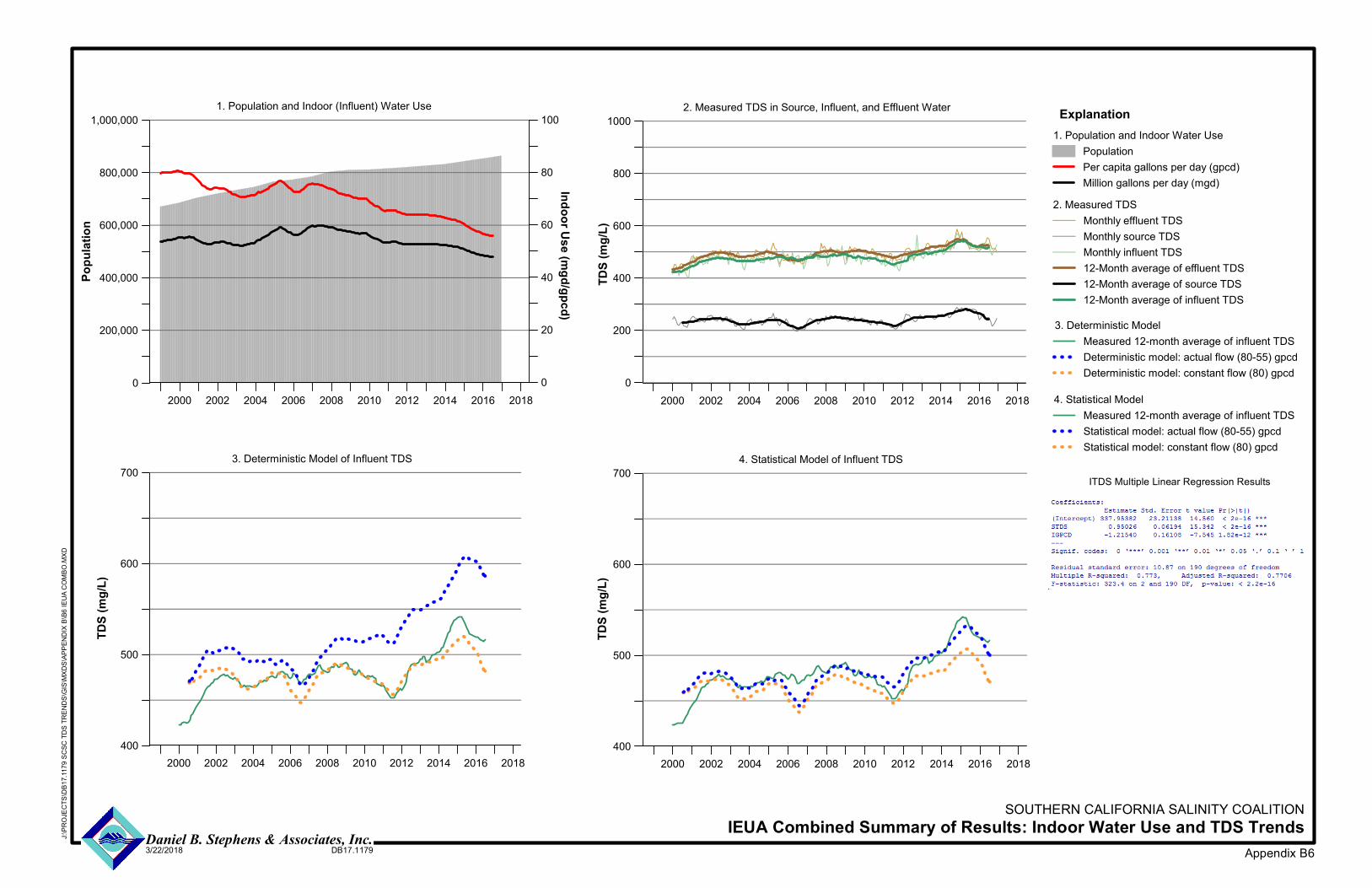
2000 2002 2004 2006 2008 2010 2012 2014 2016 20180
200,000
400,000
600,000
800,000
1,000,000
0
20
40
60
80
1001. Population and Indoor Water Use
PopulationPer capita gallons per day (gpcd)Million gallons per day (mgd)
1. Population and Indoor (Influent) Water Use
2000 2002 2004 2006 2008 2010 2012 2014 2016 20180
200
400
600
800
1000
2. Measured TDSMonthly effluent TDSMonthly source TDSMonthly influent TDS12-Month average of effluent TDS12-Month average of source TDS12-Month average of influent TDS
2. Measured TDS in Source, Influent, and Effluent WaterPo
pulat
ion
Indoor Use (mgd/gpcd)
TDS (
mg/L)
2000 2002 2004 2006 2008 2010 2012 2014 2016 2018400
500
600
700
3. Deterministic ModelMeasured 12-month average of influent TDSDeterministic model: actual flow (80-55) gpcdDeterministic model: constant flow (80) gpcd
3. Deterministic Model of Influent TDS
2000 2002 2004 2006 2008 2010 2012 2014 2016 2018400
500
600
700
4. Statistical ModelMeasured 12-month average of influent TDSStatistical model: actual flow (80-55) gpcdStatistical model: constant flow (80) gpcd
4. Statistical Model of Influent TDS
TDS (
mg/L)
TDS (
mg/L)
Explanation
Appendix B6
SOUTHERN CALIFORNIA SALINITY COALITIONIEUA Combined Summary of Results: Indoor Water Use and TDS TrendsDaniel B. Stephens & Associates, Inc.
3/22/2018 DB17.1179
J:\PR
OJEC
TS\D
B17.1
179 S
CSC
TDS T
REND
S\GIS\
MXDS
\APPE
NDIX
B\B6 I
EUA C
OMBO
.MXD
ITDS Multiple Linear Regression Results
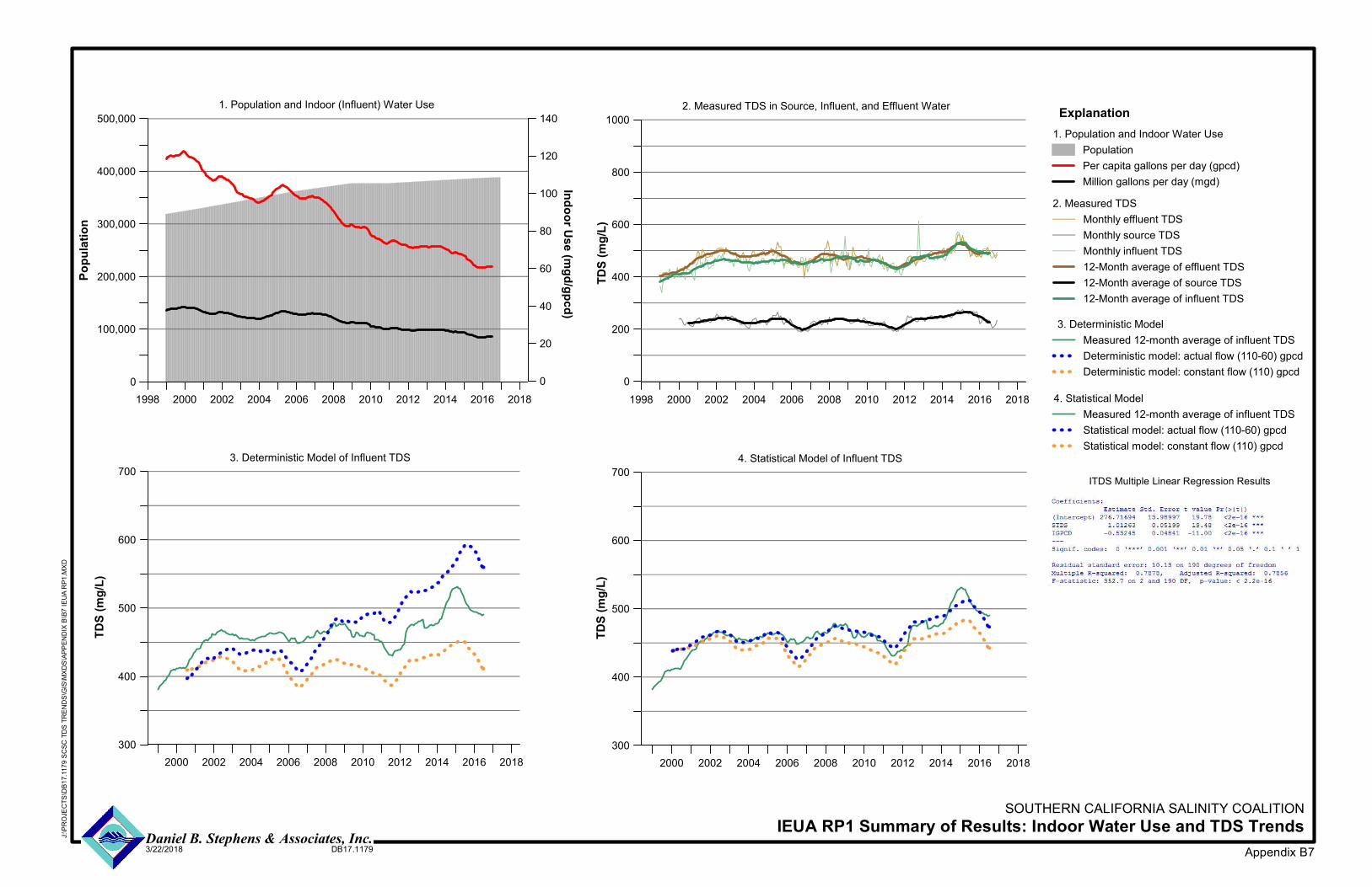
1998 2000 2002 2004 2006 2008 2010 2012 2014 2016 20180
100,000
200,000
300,000
400,000
500,000
0
40
80
120
20
60
100
1401. Population and Indoor Water Use
PopulationPer capita gallons per day (gpcd)Million gallons per day (mgd)
1. Population and Indoor (Influent) Water Use
1998 2000 2002 2004 2006 2008 2010 2012 2014 2016 20180
200
400
600
800
1000
2. Measured TDSMonthly effluent TDSMonthly source TDSMonthly influent TDS12-Month average of effluent TDS12-Month average of source TDS12-Month average of influent TDS
2. Measured TDS in Source, Influent, and Effluent WaterPo
pulat
ion
Indoor Use (mgd/gpcd)
TDS (
mg/L)
2000 2002 2004 2006 2008 2010 2012 2014 2016 2018300
400
500
600
700
3. Deterministic ModelMeasured 12-month average of influent TDSDeterministic model: actual flow (110-60) gpcdDeterministic model: constant flow (110) gpcd
3. Deterministic Model of Influent TDS
2000 2002 2004 2006 2008 2010 2012 2014 2016 2018300
400
500
600
700
4. Statistical ModelMeasured 12-month average of influent TDSStatistical model: actual flow (110-60) gpcdStatistical model: constant flow (110) gpcd
4. Statistical Model of Influent TDS
TDS (
mg/L)
TDS (
mg/L)
Explanation
Appendix B7
SOUTHERN CALIFORNIA SALINITY COALITIONIEUA RP1 Summary of Results: Indoor Water Use and TDS TrendsDaniel B. Stephens & Associates, Inc.
3/22/2018 DB17.1179
J:\PR
OJEC
TS\D
B17.1
179 S
CSC
TDS T
REND
S\GIS\
MXDS
\APPE
NDIX
B\B7 I
EUA R
P1.M
XD
ITDS Multiple Linear Regression Results
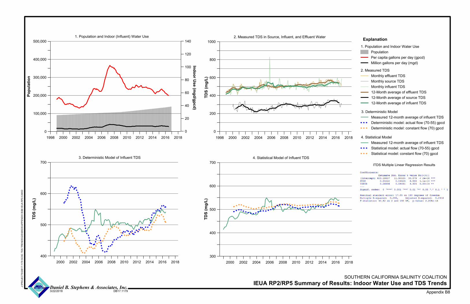
1998 2000 2002 2004 2006 2008 2010 2012 2014 2016 20180
100,000
200,000
300,000
400,000
500,000
0
40
80
120
20
60
100
1401. Population and Indoor Water Use
PopulationPer capita gallons per day (gpcd)Million gallons per day (mgd)
1. Population and Indoor (Influent) Water Use
1998 2000 2002 2004 2006 2008 2010 2012 2014 2016 20180
200
400
600
800
1000
2. Measured TDSMonthly effluent TDSMonthly source TDSMonthly influent TDS12-Month average of effluent TDS12-Month average of source TDS12-Month average of influent TDS
2. Measured TDS in Source, Influent, and Effluent WaterPo
pulat
ion
Indoor Use (mgd/gpcd)
TDS (
mg/L)
2000 2002 2004 2006 2008 2010 2012 2014 2016 2018400
500
600
700
3. Deterministic ModelMeasured 12-month average of influent TDSDeterministic model: actual flow (70-55) gpcdDeterministic model: constant flow (70) gpcd
3. Deterministic Model of Influent TDS
2000 2002 2004 2006 2008 2010 2012 2014 2016 2018300
400
500
600
700
4. Statistical ModelMeasured 12-month average of influent TDSStatistical model: actual flow (70-55) gpcdStatistical model: constant flow (70) gpcd
4. Statistical Model of Influent TDS
TDS (
mg/L)
TDS (
mg/L)
Explanation
Appendix B8
SOUTHERN CALIFORNIA SALINITY COALITIONIEUA RP2/RP5 Summary of Results: Indoor Water Use and TDS TrendsDaniel B. Stephens & Associates, Inc.
3/22/2018 DB17.1179
J:\PR
OJEC
TS\D
B17.1
179 S
CSC
TDS T
REND
S\GIS\
MXDS
\APPE
NDIX
B\B8 I
EUA R
P2-5.
MXD
ITDS Multiple Linear Regression Results
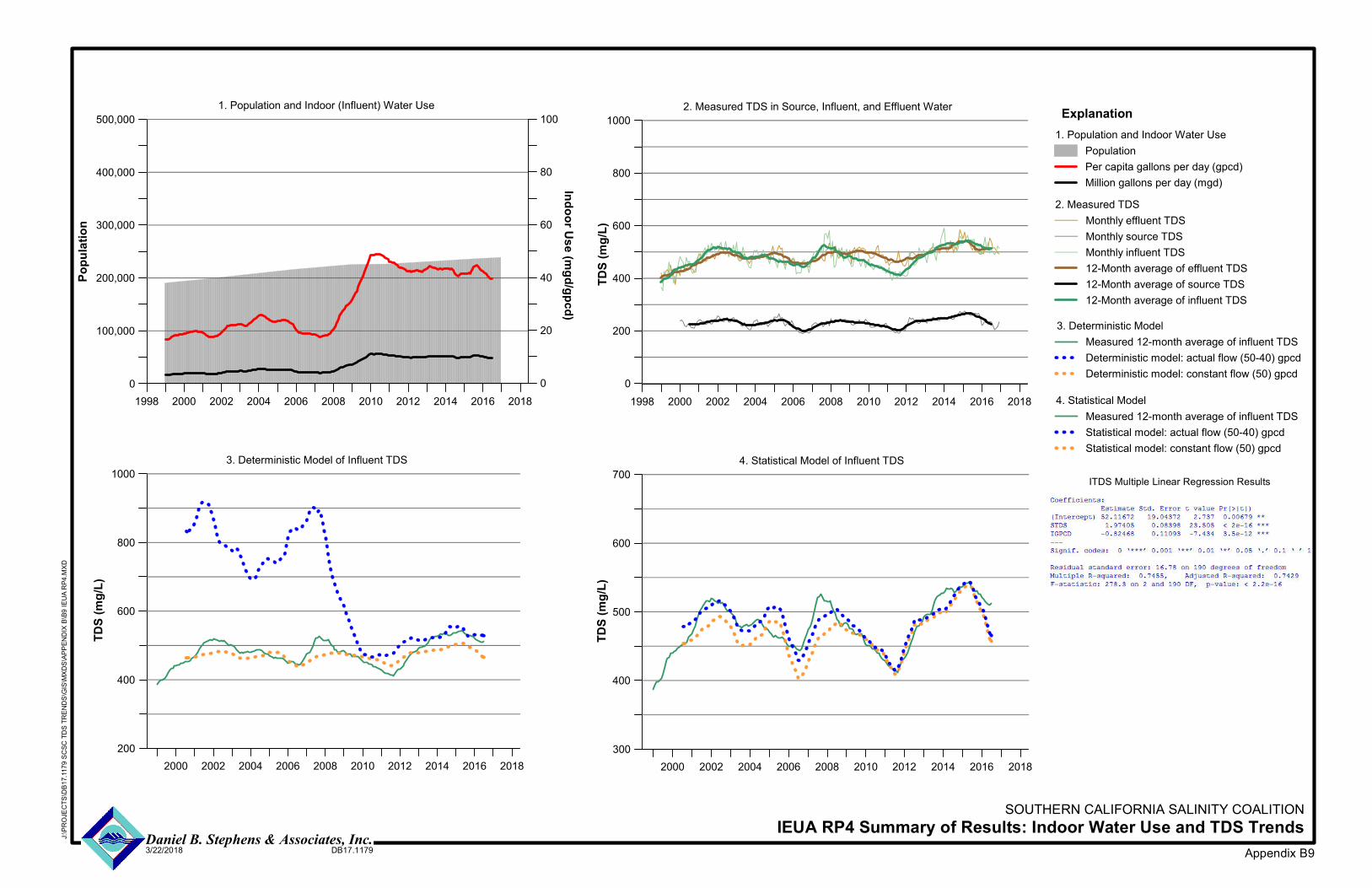
1998 2000 2002 2004 2006 2008 2010 2012 2014 2016 20180
100,000
200,000
300,000
400,000
500,000
0
20
40
60
80
1001. Population and Indoor Water Use
PopulationPer capita gallons per day (gpcd)Million gallons per day (mgd)
1. Population and Indoor (Influent) Water Use
1998 2000 2002 2004 2006 2008 2010 2012 2014 2016 20180
200
400
600
800
1000
2. Measured TDSMonthly effluent TDSMonthly source TDSMonthly influent TDS12-Month average of effluent TDS12-Month average of source TDS12-Month average of influent TDS
2. Measured TDS in Source, Influent, and Effluent WaterPo
pulat
ion
Indoor Use (mgd/gpcd)
TDS (
mg/L)
2000 2002 2004 2006 2008 2010 2012 2014 2016 2018200
400
600
800
1000
3. Deterministic ModelMeasured 12-month average of influent TDSDeterministic model: actual flow (50-40) gpcdDeterministic model: constant flow (50) gpcd
3. Deterministic Model of Influent TDS
2000 2002 2004 2006 2008 2010 2012 2014 2016 2018300
400
500
600
700
4. Statistical ModelMeasured 12-month average of influent TDSStatistical model: actual flow (50-40) gpcdStatistical model: constant flow (50) gpcd
4. Statistical Model of Influent TDS
TDS (
mg/L)
TDS (
mg/L)
Explanation
Appendix B9
SOUTHERN CALIFORNIA SALINITY COALITIONIEUA RP4 Summary of Results: Indoor Water Use and TDS TrendsDaniel B. Stephens & Associates, Inc.
3/22/2018 DB17.1179
J:\PR
OJEC
TS\D
B17.1
179 S
CSC
TDS T
REND
S\GIS\
MXDS
\APPE
NDIX
B\B9 I
EUA R
P4.M
XD
ITDS Multiple Linear Regression Results
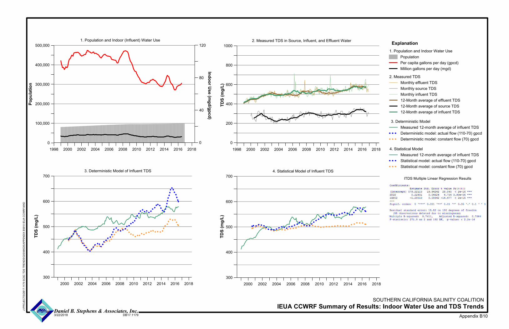
1998 2000 2002 2004 2006 2008 2010 2012 2014 2016 20180
100,000
200,000
300,000
400,000
500,000
0
40
80
1201. Population and Indoor Water Use
PopulationPer capita gallons per day (gpcd)Million gallons per day (mgd)
1. Population and Indoor (Influent) Water Use
1998 2000 2002 2004 2006 2008 2010 2012 2014 2016 20180
200
400
600
800
1000
2. Measured TDSMonthly effluent TDSMonthly source TDSMonthly influent TDS12-Month average of effluent TDS12-Month average of source TDS12-Month average of influent TDS
2. Measured TDS in Source, Influent, and Effluent Water
Popu
lation
Indoor Use (mgd/gpcd)
TDS (
mg/L)
2000 2002 2004 2006 2008 2010 2012 2014 2016 2018300
400
500
600
700
3. Deterministic ModelMeasured 12-month average of influent TDSDeterministic model: actual flow (110-70) gpcdDeterministic model: constant flow (70) gpcd
3. Deterministic Model of Influent TDS
2000 2002 2004 2006 2008 2010 2012 2014 2016 2018300
400
500
600
700
4. Statistical ModelMeasured 12-month average of influent TDSStatistical model: actual flow (110-70) gpcdStatistical model: constant flow (70) gpcd
4. Statistical Model of Influent TDS
TDS (
mg/L)
TDS (
mg/L)
Explanation
Appendix B10
SOUTHERN CALIFORNIA SALINITY COALITIONIEUA CCWRF Summary of Results: Indoor Water Use and TDS TrendsDaniel B. Stephens & Associates, Inc.
3/22/2018 DB17.1179
J:\PR
OJEC
TS\D
B17.1
179 S
CSC
TDS T
REND
S\GIS\
MXDS
\APPE
NDIX
B\B10
IEUA
CCW
RF.M
XD
ITDS Multiple Linear Regression Results
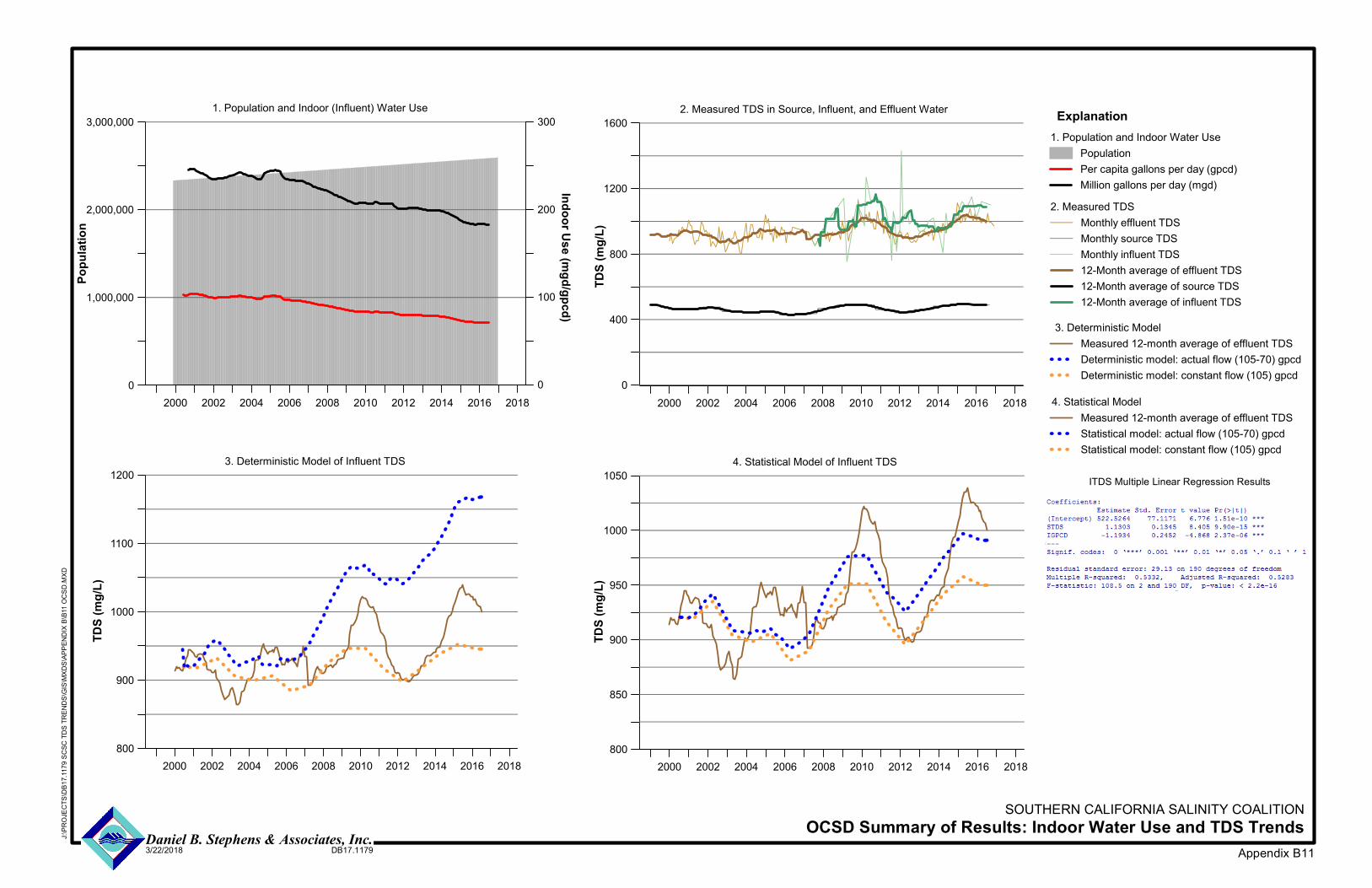
2000 2002 2004 2006 2008 2010 2012 2014 2016 20180
1,000,000
2,000,000
3,000,000
0
100
200
3001. Population and Indoor Water Use
PopulationPer capita gallons per day (gpcd)Million gallons per day (mgd)
1. Population and Indoor (Influent) Water Use
2000 2002 2004 2006 2008 2010 2012 2014 2016 20180
400
800
1200
1600
2. Measured TDSMonthly effluent TDSMonthly source TDSMonthly influent TDS12-Month average of effluent TDS12-Month average of source TDS12-Month average of influent TDS
2. Measured TDS in Source, Influent, and Effluent Water
Popu
lation
Indoor Use (mgd/gpcd)
TDS (
mg/L)
2000 2002 2004 2006 2008 2010 2012 2014 2016 2018800
900
1000
1100
1200
3. Deterministic ModelMeasured 12-month average of effluent TDSDeterministic model: actual flow (105-70) gpcdDeterministic model: constant flow (105) gpcd
3. Deterministic Model of Influent TDS
2000 2002 2004 2006 2008 2010 2012 2014 2016 2018800
850
900
950
1000
1050
4. Statistical ModelMeasured 12-month average of effluent TDSStatistical model: actual flow (105-70) gpcdStatistical model: constant flow (105) gpcd
4. Statistical Model of Influent TDS
TDS (
mg/L)
TDS (
mg/L)
Explanation
Appendix B11
SOUTHERN CALIFORNIA SALINITY COALITIONOCSD Summary of Results: Indoor Water Use and TDS TrendsDaniel B. Stephens & Associates, Inc.
3/22/2018 DB17.1179
J:\PR
OJEC
TS\D
B17.1
179 S
CSC
TDS T
REND
S\GIS\
MXDS
\APPE
NDIX
B\B11
OCS
D.MX
D
ITDS Multiple Linear Regression Results
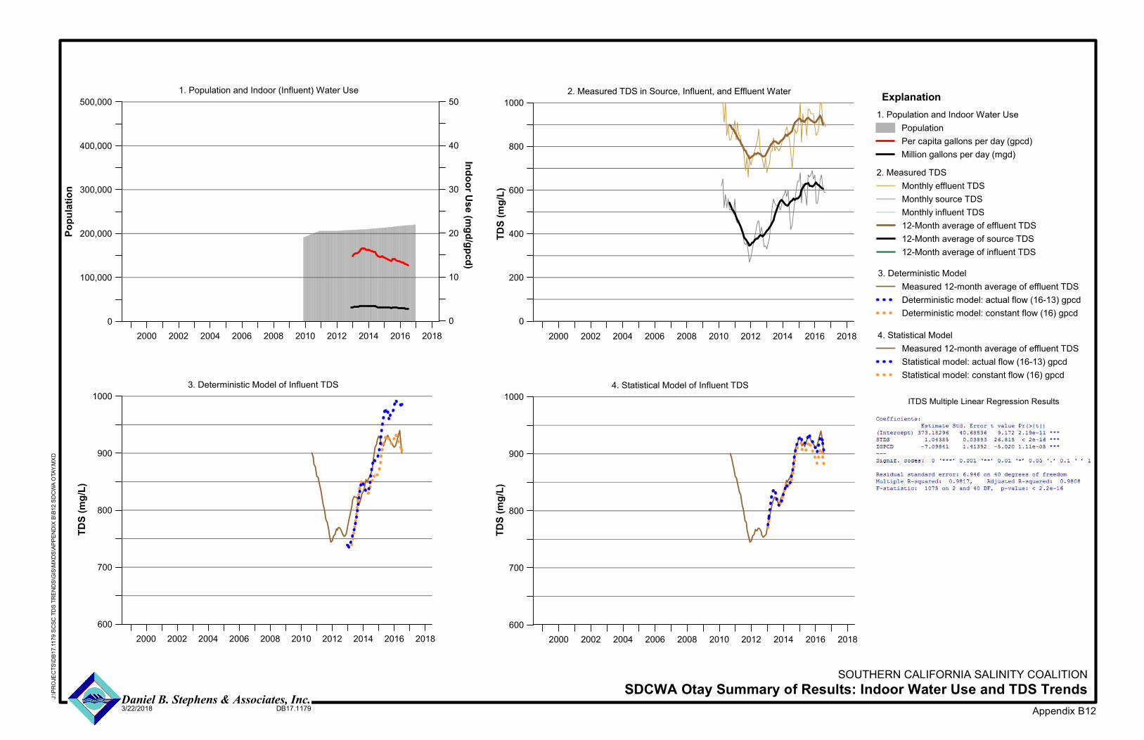
2000 2002 2004 2006 2008 2010 2012 2014 2016 20180
100,000
200,000
300,000
400,000
500,000
0
10
20
30
40
501. Population and Indoor Water Use
PopulationPer capita gallons per day (gpcd)Million gallons per day (mgd)
1. Population and Indoor (Influent) Water Use
2000 2002 2004 2006 2008 2010 2012 2014 2016 20180
200
400
600
800
1000
2. Measured TDSMonthly effluent TDSMonthly source TDSMonthly influent TDS12-Month average of effluent TDS12-Month average of source TDS12-Month average of influent TDS
2. Measured TDS in Source, Influent, and Effluent Water
Popu
lation
Indoor Use (mgd/gpcd)
TDS (
mg/L)
2000 2002 2004 2006 2008 2010 2012 2014 2016 2018600
700
800
900
1000
3. Deterministic ModelMeasured 12-month average of effluent TDSDeterministic model: actual flow (16-13) gpcdDeterministic model: constant flow (16) gpcd
3. Deterministic Model of Influent TDS
2000 2002 2004 2006 2008 2010 2012 2014 2016 2018600
700
800
900
1000
4. Statistical ModelMeasured 12-month average of effluent TDSStatistical model: actual flow (16-13) gpcdStatistical model: constant flow (16) gpcd
4. Statistical Model of Influent TDS
TDS (
mg/L)
TDS (
mg/L)
Explanation
Appendix B12
SOUTHERN CALIFORNIA SALINITY COALITIONSDCWA Otay Summary of Results: Indoor Water Use and TDS TrendsDaniel B. Stephens & Associates, Inc.
3/22/2018 DB17.1179
J:\PR
OJEC
TS\D
B17.1
179 S
CSC
TDS T
REND
S\GIS\
MXDS
\APPE
NDIX
B\B12
SDCW
A OTA
Y.MXD
ITDS Multiple Linear Regression Results
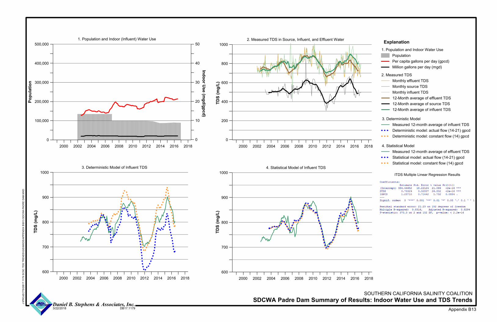
2000 2002 2004 2006 2008 2010 2012 2014 2016 20180
100,000
200,000
300,000
400,000
500,000
0
10
20
30
40
501. Population and Indoor Water Use
PopulationPer capita gallons per day (gpcd)Million gallons per day (mgd)
1. Population and Indoor (Influent) Water Use
2000 2002 2004 2006 2008 2010 2012 2014 2016 20180
200
400
600
800
1000
2. Measured TDSMonthly effluent TDSMonthly source TDSMonthly influent TDS12-Month average of effluent TDS12-Month average of source TDS12-Month average of influent TDS
2. Measured TDS in Source, Influent, and Effluent Water
Popu
lation
Indoor Use (mgd/gpcd)
TDS (
mg/L)
2000 2002 2004 2006 2008 2010 2012 2014 2016 2018600
700
800
900
1000
3. Deterministic ModelMeasured 12-month average of influent TDSDeterministic model: actual flow (14-21) gpcdDeterministic model: constant flow (14) gpcd
3. Deterministic Model of Influent TDS
2000 2002 2004 2006 2008 2010 2012 2014 2016 2018600
700
800
900
1000
4. Statistical ModelMeasured 12-month average of effluent TDSStatistical model: actual flow (14-21) gpcdStatistical model: constant flow (14) gpcd
4. Statistical Model of Influent TDS
TDS (
mg/L)
TDS (
mg/L)
Explanation
Appendix B13
SOUTHERN CALIFORNIA SALINITY COALITIONSDCWA Padre Dam Summary of Results: Indoor Water Use and TDS TrendsDaniel B. Stephens & Associates, Inc.
3/22/2018 DB17.1179
J:\PR
OJEC
TS\D
B17.1
179 S
CSC
TDS T
REND
S\GIS\
MXDS
\APPE
NDIX
B\B13
SDCW
A PAD
RE D
AM.M
XD
ITDS Multiple Linear Regression Results
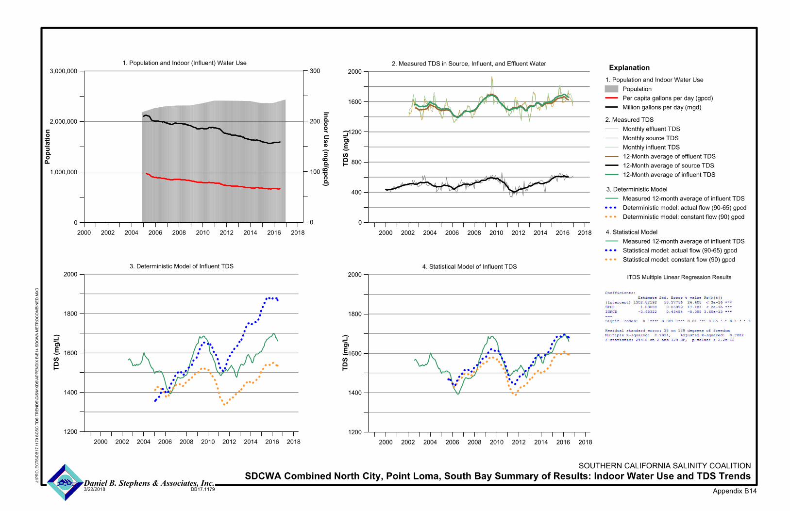
2000 2002 2004 2006 2008 2010 2012 2014 2016 20180
1,000,000
2,000,000
3,000,000
0
100
200
3001. Population and Indoor Water Use
PopulationPer capita gallons per day (gpcd)Million gallons per day (mgd)
1. Population and Indoor (Influent) Water Use
2000 2002 2004 2006 2008 2010 2012 2014 2016 20180
400
800
1200
1600
2000
2. Measured TDSMonthly effluent TDSMonthly source TDSMonthly influent TDS12-Month average of effluent TDS12-Month average of source TDS12-Month average of influent TDS
2. Measured TDS in Source, Influent, and Effluent Water
Popu
lation
Indoor Use (mgd/gpcd)
TDS (
mg/L)
2000 2002 2004 2006 2008 2010 2012 2014 2016 20181200
1400
1600
1800
2000
3. Deterministic ModelMeasured 12-month average of influent TDSDeterministic model: actual flow (90-65) gpcdDeterministic model: constant flow (90) gpcd
3. Deterministic Model of Influent TDS
2000 2002 2004 2006 2008 2010 2012 2014 2016 20181200
1400
1600
1800
2000
4. Statistical ModelMeasured 12-month average of influent TDSStatistical model: actual flow (90-65) gpcdStatistical model: constant flow (90) gpcd
4. Statistical Model of Influent TDS
TDS (
mg/L)
TDS (
mg/L)
Explanation
Appendix B14
SOUTHERN CALIFORNIA SALINITY COALITIONSDCWA Combined North City, Point Loma, South Bay Summary of Results: Indoor Water Use and TDS TrendsDaniel B. Stephens & Associates, Inc.
3/22/2018 DB17.1179
J:\PR
OJEC
TS\D
B17.1
179 S
CSC
TDS T
REND
S\GIS\
MXDS
\APPE
NDIX
B\B14
SDCW
A MET
ROCO
MBIN
ED.M
XD
ITDS Multiple Linear Regression Results