Stateful Programming of High-Speed

Network Hardware

Mina Tahmasbi Arashloo

A Dissertation

Presented to the Faculty

of Princeton University

in Candidacy for the Degree

of Doctor of Philosophy

Recommended for Acceptance

by the Department of

Computer Science

Adviser: Professor Jennifer Rexford

June 2019

© Copyright by Mina Tahmasbi Arashloo, 2019.

All rights reserved.

Abstract

Modern networks need to operate at speeds as high as 100Gbps while running sophis-

ticated algorithms and protocols to provide strict performance, security and reliability

guarantees. Moreover, they need to flexibly adapt to the rapidly evolving require-

ments of online services. Thus, emerging network hardware devices, i.e. switches

inside the network and Network Interface Cards (NICs) at the end hosts, are high-

speed and programmable, with on-chip memory accessible on a per-packet basis to

support stateful packet processing.

However, the programming interfaces of these devices are quite low-level, tied to

each device’s architecture, and only suitable for programming a single device. Thus,

programming collections of stateful network devices to realize a local or network-wide

functionality efficiently and correctly is extremely difficult and error-prone. This

dissertation focuses on the design and implementation of high-level programming

abstractions for stateful programming of high-speed network hardware, both at the

end hosts and inside the network.

At the end host, we focus on the transport layer, the most complicated, constantly-

evolving, and stateful component of the network stack. Transport-layer algorithms

maintain state across packets to decide what data segments to transmit and when,

and are notoriously difficult to implement on programmable NICs at high-speed.

We propose Tonic, a hardware architecture for transport algorithms that can sup-

port 100Gbps for 128-byte packets while being programmable with a simple API.

In designing Tonic, we exploit common patterns across transport algorithms to cre-

ate efficient fixed-function reusable hardware modules, thus significantly reducing the

functionality programmers must specify.

To facilitate network-wide stateful programming, we propose SNAP, a program-

ming language that abstracts the entire network as “one big stateful switch”. Using

SNAP, operators can program using persistent arrays on one big switch without de-iii

ciding how to distribute and access them in the network’s switches. The SNAP

compiler discovers read/write dependencies between arrays, translates one-big-switch

programs into an efficient internal representation based on binary decision diagrams,

and uses it to jointly optimize array placement and routing across the network.

All in all, Tonic’s modular interface and SNAP’s one-big-stateful-switch abstrac-

tion relieve programmers from the low-level details of stateful programming of high-

speed network hardware throughout the entire network.

iv

Acknowledgments

I am beyond grateful to my PhD advisor, Jennifer Rexford, for her unparalleled

support, guidance, and mentorship throughout my PhD program. I have learned so

many invaluable lessons from Jen: how to find the right problems to solve, how to

think critically without getting caught up in irrelevant details, how to present my

ideas concisely and elegantly, and how to gracefully navigate through technical and

professional difficulties. Jen has always wholeheartedly encouraged and supported

me to search for my passions and has been there every step of the way to help me in

their pursuit. I am a different person today, both professionally and personally, than

I was when I started this journey and for that, I am forever in her debt.

I would like to deeply thank David Walker, who has been like a second advisor to

me. My first major research project started from his graduate seminar and evolved

into the third chapter of this dissertation. Dave has always provided me with invalu-

able guidance on approaching research problems and writing papers, and has strongly

supported me throughout this process.

I thank the other members of my committee, Arvind Krishnamurthy, Nick Feam-

ster, and Michael Freedman, for their helpful feedback and insightful discussions that

significantly improved the quality of this dissertation. I am also grateful to Aarti

Gupta for introducing me to the fundamentals of software verification and how it can

be used to build more reliable networks. I profoundly enjoyed her course and our

several discussions on network verification.

I have had the privilege of working with great collaborators in the past few years.

Srinivas Narayana has been an amazing mentor, collaborator, and friend. I joined

his Path Queries project in my first semester as a PhD student. He showed me how

to be patient and believe in my ideas, and how to cheerfully embrace the inherent

uncertainty of research. I am grateful to Alexey Lavrov, who patiently helped me

build my background on hardware design, and spent countless hours discussing thev

project in the second chapter of this dissertation with me. I had great pleasure

working with Yaron Koral and Michael Greenberg on the project in the third chapter

of this dissertation and learned a lot from both. I also thank Rohan Gandhi, Manya

Ghobadi, Guohan Lu, Pavel Shirshov, David Wentzlaff, and Lihua Yuan.

Special thanks to Victor Bahl, Hari Balakrishnan, Daniel Firestone, Hongqiang

Liu, Jitendra Padhye, and Anirudh Sivaraman for eye-opening discussions and advice

on research and professional life. I am also grateful to Mitra Kelly, for her generous

help with the administrative work these years, and to Nicki Mahler, the graduate

coordinator at Princeton’s CS department, for always being available, welcoming,

and tremendously helpful, and all the fun conversations about our dogs.

I would like to further acknowledge the National Science Foundation awards CNS-

1704077, CCF-1535948, and CNS-1162112, DARPA contract HR0011-17-C-0047, the

Open Technology Fund 1002-2017-045, the Siebel Scholars Foundation, and Microsoft

Research Dissertation Grant for funding the work presented in this dissertation.

I am extremely grateful to the amazing members of my Cabernet family for their

constant professional and personal support, and for making this journey so satisfying

and fun. Special thanks to Rob Harrison, for memorable conversations about literally

anything from research to day-to-day life to the humankind, and for cheering me on

to the finish line, to Robert MacDavid, for sharing my passion about animals which

brought about some of the most enjoyable moments of my time at Princeton, and to

Shir Landau-Feibish, for her positivity and constant encouragement and support.

To my dear friends at Princeton, Hamid, Raissa, Sameer, Rutwik, Melissa, Moein,

Luciano, and Laura, thank you for all the long game nights, movie nights, birthdays,

get togethers, and trips over these years, and the fun first year we spent at GC

together. You have been my support system away from my family, always there to

celebrate the ups and cheer me up in the downs. My time at Princeton would not

have been half as special and joyful without you.

vi

To my parents, Ata and Parvin, and my sister, Maryam, I am forever in your

debt for all your sacrifices and your unconditional love and support. You were the

first to encourage me to think critically, not to take anything for granted, and to ask

questions. Thank you for being there for me every minute of every day, even from

thousands of miles away. To the furry four-legged ruler of my life, Shasta, thank you

for bringing so much joy and happiness into my life and making me a better person

in your own special way. Finally, to my incredible partner in crime, Sepehr, thank

you for your unbounded love and support, for facing the craziness of the world with

me, and for making me grow every single day. This would not have been possible

without you.

vii

To my parents, for their boundless love,

Maryam, the best sister one can ever ask for,

and Sepehr, for always being by my side.

viii

Contents

Abstract . . . . . . . . . . . . . . . . . . . . . . . . . . . . . . . . . . . . . iii

Acknowledgments . . . . . . . . . . . . . . . . . . . . . . . . . . . . . . . . v

List of Tables . . . . . . . . . . . . . . . . . . . . . . . . . . . . . . . . . . xiii

List of Figures . . . . . . . . . . . . . . . . . . . . . . . . . . . . . . . . . . xiv

Bibliographic Notes . . . . . . . . . . . . . . . . . . . . . . . . . . . . . . . xv

1 Introduction 1

1.1 Motivating Examples . . . . . . . . . . . . . . . . . . . . . . . . . . . 6

1.1.1 Reliable Transport . . . . . . . . . . . . . . . . . . . . . . . . 6

1.1.2 Network Telemetry . . . . . . . . . . . . . . . . . . . . . . . . 8

1.1.3 Network Functions . . . . . . . . . . . . . . . . . . . . . . . . 9

1.2 Modern Programmable Network Hardware . . . . . . . . . . . . . . . 11

1.2.1 Programmable Hardware Inside the Network . . . . . . . . . . 13

1.2.2 Programmable Hardware at the End Hosts . . . . . . . . . . . 14

1.3 The Challenges of Stateful Programming in High-Speed Networks . . 15

1.3.1 Stateful Programming of a Single Device . . . . . . . . . . . . 15

1.3.2 Network-Wide Stateful Programming . . . . . . . . . . . . . . 18

1.4 Contributions . . . . . . . . . . . . . . . . . . . . . . . . . . . . . . . 19

1.4.1 Tonic: Stateful Programming of Hardware Network Stacks . . 19

1.4.2 SNAP: Network-Wide Stateful Programming . . . . . . . . . . 20

ix

2 Tonic: Stateful Programming of Hardware Network Stacks 22

2.1 Tonic as the Transport Logic . . . . . . . . . . . . . . . . . . . . . . . 26

2.2 Hardware Design Challenges . . . . . . . . . . . . . . . . . . . . . . . 30

2.3 Common Patterns in Transport Logic . . . . . . . . . . . . . . . . . . 31

2.3.1 Segment Selection Patterns . . . . . . . . . . . . . . . . . . . 31

2.3.2 Credit Management Patterns . . . . . . . . . . . . . . . . . . 35

2.4 Tonic Architecture . . . . . . . . . . . . . . . . . . . . . . . . . . . . 38

2.4.1 Efficient Flow Scheduling . . . . . . . . . . . . . . . . . . . . . 39

2.4.2 Flexible Segment Selection . . . . . . . . . . . . . . . . . . . . 41

2.4.3 Flexible Credit Management . . . . . . . . . . . . . . . . . . . 46

2.4.4 Handling Conflicting Events . . . . . . . . . . . . . . . . . . . 48

2.5 Tonic’s Programming Interface . . . . . . . . . . . . . . . . . . . . . . 49

2.6 Hardware Implementation . . . . . . . . . . . . . . . . . . . . . . . . 50

2.6.1 High-Precision Per-Flow Rate Limiting . . . . . . . . . . . . . 50

2.6.2 Efficient Bitmap Operations . . . . . . . . . . . . . . . . . . . 51

2.6.3 Concurrent Memory Reads and Writes . . . . . . . . . . . . . 52

2.7 Integrating Tonic into the Transport Layer . . . . . . . . . . . . . . . 53

2.7.1 Linux Kernel and Socket API . . . . . . . . . . . . . . . . . . 53

2.7.2 RDMA NICs and Verbs API . . . . . . . . . . . . . . . . . . . 56

2.8 Evaluation . . . . . . . . . . . . . . . . . . . . . . . . . . . . . . . . . 58

2.8.1 Hardware Design . . . . . . . . . . . . . . . . . . . . . . . . . 59

2.8.2 End-to-End Behavior . . . . . . . . . . . . . . . . . . . . . . . 64

2.9 Related Work . . . . . . . . . . . . . . . . . . . . . . . . . . . . . . . 67

2.10 Conclusions . . . . . . . . . . . . . . . . . . . . . . . . . . . . . . . . 68

3 SNAP: Network-Wide Stateful Programming 70

3.1 Overview . . . . . . . . . . . . . . . . . . . . . . . . . . . . . . . . . . 73

3.1.1 Writing Network-Wide Stateful Programs . . . . . . . . . . . 73x

3.1.2 Distributing Programs across the Network . . . . . . . . . . . 78

3.2 The SNAP Language . . . . . . . . . . . . . . . . . . . . . . . . . . . 81

3.2.1 Predicates . . . . . . . . . . . . . . . . . . . . . . . . . . . . . 83

3.2.2 Policies. . . . . . . . . . . . . . . . . . . . . . . . . . . . . . . 85

3.3 Example SNAP Programs . . . . . . . . . . . . . . . . . . . . . . . . 88

3.4 The SNAP Compiler . . . . . . . . . . . . . . . . . . . . . . . . . . . 96

3.4.1 State Dependency Analysis . . . . . . . . . . . . . . . . . . . 97

3.4.2 Extended Forwarding Decision Diagrams . . . . . . . . . . . . 98

3.4.3 Packet-State Mapping . . . . . . . . . . . . . . . . . . . . . . 107

3.4.4 State Placement and Routing . . . . . . . . . . . . . . . . . . 108

3.4.5 Generating Switch Configurations . . . . . . . . . . . . . . . . 112

3.5 Implementation . . . . . . . . . . . . . . . . . . . . . . . . . . . . . . 114

3.6 Evaluation . . . . . . . . . . . . . . . . . . . . . . . . . . . . . . . . . 117

3.6.1 Language Expressiveness . . . . . . . . . . . . . . . . . . . . . 117

3.6.2 Compiler Performance . . . . . . . . . . . . . . . . . . . . . . 118

3.7 Discussion . . . . . . . . . . . . . . . . . . . . . . . . . . . . . . . . . 123

3.7.1 SNAP and Middleboxes . . . . . . . . . . . . . . . . . . . . . 124

3.7.2 Extending SNAP . . . . . . . . . . . . . . . . . . . . . . . . . 125

3.8 Related Work . . . . . . . . . . . . . . . . . . . . . . . . . . . . . . . 127

3.9 Conclusion . . . . . . . . . . . . . . . . . . . . . . . . . . . . . . . . . 130

4 Conclusion 131

4.1 Summary of Contributions . . . . . . . . . . . . . . . . . . . . . . . . 132

4.2 Future Directions . . . . . . . . . . . . . . . . . . . . . . . . . . . . . 133

4.2.1 Reasoning across Multiple Flows in the Transport Layer . . . 133

4.2.2 Accelerating Networked Applications . . . . . . . . . . . . . . 134

4.2.3 Network-Wide Programming at Multiple Abstraction Levels . 135

4.2.4 Programming a Network of Heterogeneous Devices . . . . . . 136xi

4.3 Final Remarks . . . . . . . . . . . . . . . . . . . . . . . . . . . . . . . 136

Bibliography 138

xii

List of Tables

2.1 Common transport logic patterns . . . . . . . . . . . . . . . . . . . . 32

2.2 Per-flow state variables in Tonic’s segment selection engine . . . . . . 44

2.3 Resource utilization of the transport logic of various protocols in Tonic 61

2.4 Summary of Tonic’s scalability results . . . . . . . . . . . . . . . . . . 64

3.1 Applications written in SNAP . . . . . . . . . . . . . . . . . . . . . . 89

3.2 Inputs and outputs of SNAP’s optimization problem . . . . . . . . . 109

3.3 Constraints of the optimization problem . . . . . . . . . . . . . . . . 111

3.4 SNAP compiler phases and their execution in different scenarios . . . 119

3.5 Enterprise/ISP topologies used for evaluating SNAP’s compiler . . . . 120

3.6 Runtime of SNAP’s compiler phases for a sample program . . . . . . 120

xiii

List of Figures

1.1 Packet processing in early networks vs modern networks . . . . . . . 3

1.2 Evolution of Ethernet standard speeds . . . . . . . . . . . . . . . . . 5

2.1 Tonic in a hardware network stack on the NIC . . . . . . . . . . . . . 29

2.2 Tonic’s architecture . . . . . . . . . . . . . . . . . . . . . . . . . . . . 38

2.3 NewReno’s Tonic vs hard-coded implementation in NS3 . . . . . . . . 65

2.4 RoCEv2 with DCQCN in Tonic vs hard-coded in NS3 . . . . . . . . . 67

3.1 Example topology for SNAP’s running example . . . . . . . . . . . . 76

3.2 The xFDD for SNAP’s running example . . . . . . . . . . . . . . . . 79

3.3 SNAP’s syntax . . . . . . . . . . . . . . . . . . . . . . . . . . . . . . 82

3.4 Overview of SNAP’s compiler phases . . . . . . . . . . . . . . . . . . 97

3.5 SNAP’s compiler function for determining state variable dependencies 98

3.6 SNAP’s xFDD syntax . . . . . . . . . . . . . . . . . . . . . . . . . . 100

3.7 Translating SNAP programs into xFDDs . . . . . . . . . . . . . . . . 102

3.8 xFDD composition operators . . . . . . . . . . . . . . . . . . . . . . . 103

3.9 A closer look at the ⊕ operator for xFDD composition . . . . . . . . 104

3.10 Compilation time of an example policy on enterprise/ISP networks . 121

3.11 Compilation time of an example policy on synthesized topologies . . . 121

3.12 Compilation time for 20 incrementally-composed policies . . . . . . . 122

xiv

Bibliographic Notes

The material presented in chapter 2 is a joint work with Alexey Lavrov, Manya

Ghobadi, Jennifer Rexford, David Walker, and David Wentzlaff. The material pre-

sented in chapter 3 has been previously published and publicly presented at ACM

SIGCOMM 2016 [100], has appeared in an arXiv paper [99] and a Princeton CS

department technical report [101], and is a joint work with Yaron Koral, Michael

Greenberg, Jennifer Rexford, and David Walker.

xv

Chapter 1

Introduction

Computer networks are fundamental to enabling online service that we use every day

such as search engines, social media, video streaming, and mobile banking. Online

services are hosted in data centers, using clusters of compute servers to process and

respond to user requests. When a user requests a service, e.g., fetching a webpage

or looking up a phrase in a search engine, enterprise and transit networks transfer

the request to the data center hosting that service. Within the data center, servers

use the data center’s network to communicate and collectively compute a response,

which is carried back to the user by transit and enterprise networks. As a result, the

performance, security, and availability of online services is strongly tied to those of

the underlying computer networks.

As online services become more prevalent, designing and operating computer net-

works gets more challenging. Today, computer networks must provide connectivity

at an unprecedented scale: they must transfer large volumes of data at high speed

between billions of user devices and thousands of online services. Moreover, there

are constantly new kinds of devices and services that need network connectivity, each

with different requirements in terms of network performance, security, and availabil-

ity. For instance, most Internet of Things (IoT) devices do not need high bandwidth

1

or low latency network connections. However, they benefit from network-provided

security as they are low-power devices with low computational capabilities and not

suitable for implementing many attack detection and mitigation mechanisms them-

selves. As another example, servers processing search requests in data centers require

low-latency network communications to provide answers as fast as possible. On the

other hand, storage clusters, which store the data used by the compute servers in

data centers, require both high-bandwidth and low-latency network communications.

To support such diversity and scale, network operators need to design the “right”

set of algorithms (to run on individual network devices) and protocols (for network

devices to coordinate) that can provide the communication properties expected by

the services and devices using the network. More specifically, depending on the per-

formance, security, and availability requirements of services and user devices, these

algorithms and protocols need to detect various forms of congestion, security attacks,

and device failures, and react by adjusting how traffic streams are routed to their des-

tination, blocking malicious traffic, and swiftly recovering from failures. As new kinds

of devices and services connect to networks, network algorithms and protocols evolve

to accommodate their performance, security and availability requirements. This, as

we describe below, has driven the underlying hardware that runs these algorithms

and protocols for processing packets to evolve as well.

Early networks did not face as wide-ranging and strict requirements on perfor-

mance, security, and availability as networks do today. They were designed to only

provide best-effort packet delivery inside the network, where network devices must

process larger volumes of traffic, and leave more complicated algorithms and pro-

tocols to run at the edge on the end hosts (the end-to-end argument [86]). As a

result, network hardware in switches and routers, i.e., devices inside the network,

used to only perform stateless packet processing, which is simple, sufficient for run-

ning algorithms and protocols that provide best-effort packet delivery, and amenable

2

(a) Early networks

(b) Modern networks

Figure 1.1: Packet processing in early networks (a) vs modern networks (b)

to efficient hardware implementations. In stateless packet processing, each packet is

processed independently from others, using only the information inside the packet’s

headers to decide how to forward it to its final destination.

The more sophisticated algorithms and protocols, which provided functionalities

such as reliable transport and stateful firewalls, used to run in software at the end

hosts. These algorithms and protocols typically require stateful packet processing, i.e.,

maintaining information across packets and using it for processing incoming traffic.

Given the lower link speeds at the time, these algorithms and protocols could run on

the general-purpose CPU at the end host without significant CPU overhead, using the

end-host memory for maintaining state across packets. Thus, the network interface

card (NIC) at the end host was only used to perform stateless algorithms and protocols

3

in the link and physical layers before transmitting packets into the network. Overall,

specialized network hardware, i.e., switches inside the network and NICs at the end

hosts, used to perform stateless packet processing, whereas stateful packet processing

was implemented on the CPU at the end hosts (Figure 1.1a).

This distinction, however, is fading in modern networks as they are increasingly

forced to run algorithms and protocols that require stateful packet processing, both

inside the network and at the end hosts, at high speed (Figure 1.1b). With the

growing diversity and scale of online services, stateless packet processing inside the

network is no longer sufficient for running algorithms and protocols that can provide

the required levels of performance, security, and reliability (see section 1.1 for detailed

examples). Moreover, as data centers move to higher link speeds, i.e., 40Gbps and

100Gbps Ethernet, the CPU overhead of processing packets in software is becoming

prohibitive. Thus, more sophisticated algorithms and protocols, including those that

require stateful packet processing such as reliable transport, are forced to run in the

NIC [17,24, 58]. On the other hand, as mentioned above and discussed via examples

in section 1.1, network operators need to constantly adapt network algorithms and

protocols to the ever-evolving performance, security, and availability requirements of

their users. Thus, modern networks need hardware that is:

• high speed, i.e., can keep up with the increasing link speed. Link speeds have

been rapidly increasing over the past decade from 10Gbps, to 40Gbps, and more

recently 100Gbps Ethernet (Figure 1.2). The IEEE standards for 200Gbps and

400Gbps Ethernet have recently been released as well, with commercial products

operating at this speed to follow in the coming years. To keep up with this

increasing line rate, network devices need to transmit a processed data packet

every few nanoseconds.

• capable of stateful packet processing, i.e., can maintain state across packets and

use it in processing incoming traffic.4

1980

1985

1990

1995

2000

2005

2010

2015

2020

Year

101

102

103

104

105

Sta

ndard

Speed

(M

bbps,

log s

cale

)

10Mbps

100Mbps

1Gbps

10Gbps

40Gbps

100Gbps 200Gbps

400Gbps

Figure 1.2: Evolution of Ethernet standard speeds. Dates refer to the year the IEEEstandard for the corresponding speeds was released (not all the standards are shown).

• programmable, i.e., its packet-processing behavior can be specified by network

operators through a programming interface.

These requirements have resulted in the design and development of several pro-

grammable network hardware devices with on-chip memory accessible on a per-packet

basis in the past few years [15,19,25,44,68,69,103].

However, as we discuss in section 1.2, supporting stateful packet processing and

providing programmability both become increasingly difficult at higher speeds. As

a result, these devices are constrained in the set of stateless and stateful per-packet

operations they support at high speed. That is, each device makes its own compro-

mises in the set of algorithms and protocols to optimize its architecture for. This,

as we discuss in section 1.3, makes it challenging to use these devices to implement

stateful algorithms and protocols correctly and efficiently. To do so, network oper-

ators need to acquire deep knowledge about each device’s architecture and memory

layout, program using low-level instruction sets, and refactor and/or optimize their

implementation of stateful algorithms and protocols accordingly. Programming a col-

lection of devices is even more difficult as network operators have to reason about

how to partition and manage the state across multiple devices as well.

5

This dissertation focuses on the design and implementation of high-level program-

ming abstractions for network algorithms and protocols that require stateful packet

processing on modern high-speed programmable network hardware. We identify the

common patterns across several stateful algorithms and protocols that are required

for operating modern networks, both at the end hosts and inside the network. Using

these patterns, we design modular and high-level interfaces for stateful programming

of individual as well as collections of high-speed network hardware (see section 1.4

for an overview).

More specifically, we relieve programmers from dealing with the low-level hard-

ware details by either (i) designing a high-level programming language and a compiler

to automatically translate it to low-level hardware components, or (ii) significantly

reducing the functionality programmers must specify by developing efficient hardware

components that can be reused across several algorithms and protocols. We demon-

strate that our programming interfaces are expressive enough to support a wide range

of algorithms and protocols while being amenable to efficient implementation on mod-

ern network hardware.

1.1 Motivating Examples

In this section, we discuss three categories of algorithms and protocols that evolved

over time to require stateful and programmable packet processing on high speed

hardware.

1.1.1 Reliable Transport

The transport layer sits between the applications and the rest of the network stack

at the end hosts. It implements a transport protocol, which specifies how to enable

communication between applications on remote end hosts. More specifically, trans-

port protocols use two main algorithms, namely data delivery and congestion control

6

algorithms, to determine how to transfer data from one application to another in a

stream of data segments reliably and efficiently. Data delivery algorithms determine

which set of bytes from the application original data constitute the next transmit-

ted data segment, and congestion control algorithms determine when each segment

should be released into the network.

Transport-layer algorithms typically require stateful packet processing. Data de-

livery algorithms keep per-flow state to keep track of the delivery status of data

segments. The state is updated when a segment from the flow is transmitted into the

network or if an acknowledgement is received, and is used, for instance, to detect lost

segments and decide whether to transmit new data in the next segment or retransmit

lost data. Congestion control algorithms maintain state across packets as well (e.g.,

an estimation of round trip time for each flow, current and target congestion window

or rate, and state machines to track their observed network state) to keep track of the

available network capacity and adjust the pace at which data segments are released

into the network.

Moreover, programmability is crucial to the algorithms in the transport layer.

Using the “right” algorithms in the transport layer is central to achieving high per-

formance as these algorithms control how data is released into the network. As

such, since the introduction of TCP in the 1970s, there has been constant innova-

tion in designing data delivery and congestion control algorithms to improve the

performance of network transport for various kinds of networks and applications

[3, 10, 14,21,29,38,48,55,60,61,64,104,109].

Until recently, the transport layer, along with the rest of the network stack, used

to be implemented in software on the end-host’s CPU, which naturally provided the

required stateful and programmable packet processing for data delivery and conges-

tion control algorithms. However, as data center networks move to higher link speeds,

i.e., 40Gbps and 100Gbps Ethernet, the CPU overhead of packet processing in soft-

7

ware becomes prohibitive. Thus, there is an increasing effort to offload the end-host’s

network stack, including the transport layer, to the hardware on the NIC [16,17,58].

As such, the combination of increasing link speeds in data centers and the stateful

and ever-evolving nature of transport layer algorithms is an indication of the need

for high-speed programmable hardware with support for stateful packet processing in

modern networks.

1.1.2 Network Telemetry

Network telemetry consists of a set of protocols and algorithms for conducting mea-

surements across the network to provide visibility into and answer queries about the

state of the network in a fine-grained and timely fashion. More specifically, telemetry

systems decide how and where in the network to collect data and statistics to answer

questions about what goes on in the network, e.g., flow-size distributions, transient

and long-term congestion, distributed denial of service (DDoS) attacks, and failures.

As such, they are a crucial component of network management and have been studied

extensively.

Network telemetry requires stateful packet processing: computing any non-trivial

statistics across the network, e.g., flow sizes, top-k heavy hitter flows, and number of

unique flows, requires accumulating information across packets. Detecting heavy hit-

ter flows, for instance, requires approximate data structures that can efficiently track

and sort the total number of recently received packets for potentially millions of flows.

Moreover, telemetry systems need to be flexible: network operators’ queries about

the network can vary over time depending on the observed network behavior from

previous queries (shorter time scale), and the security, and availability requirements

of the user devices and services using that network (longer time scale).

Early networks did not face as wide-ranging and strict requirements on perfor-

mance, security, and availability as networks do today. Thus, they could afford slower

8

detection of and reaction to congestion, attacks, and failures. Moreover, they operated

at much lower link speeds. Thus, early network telemetry systems, e.g., sFlow [87]

and NetFlow [67], only perform a limited amount of stateful packet processing in

the switch to record a fixed set of statistics over the (sometimes sampled) stream of

packets in a pre-defined time interval. The records are then periodically sent to an

off-path central location for more comprehensive and sophisticated analysis to answer

a range of queries.

However, periodic reporting of a small fixed set of statistics every few seconds is not

sufficient for managing modern networks. Satisfying the strict network requirements

of today’s services requires real-time detection and reaction to network events such as

congestion, attacks, and failures. Moreover, increasing link speeds make it infeasible

to further increase the frequency of reporting. As a result, there has been a growing

effort to offload more of the off-path stateful analysis to the switches in the network

[35, 51, 66, 107]. More specifically, instead of recording a small fixed set of statistics,

these telemetry systems derive the information that should be maintained across

packets to answer the operator’s query. Thus, network telemetry in modern networks

requires programmable stateful packet processing on high-speed to answer wide ranges

of queries about the network in real time.

1.1.3 Network Functions

With the growing diversity and scale of online services, best-effort packet delivery

using stateless packet processing inside the network is no longer sufficient for providing

the required levels of performance, security, and reliability. Today, network operators

need to run stateful “functions” inside the network: layer-4 load balancers that map

connections to web servers on the fly while keeping track of the mapping to ensure

connection affinity and balanced load, intrusion detection systems (IDSs) and stateful

firewalls to detect security attacks that require reasoning across packet boundaries,

9

proxies to terminate insecure connections and initiate secure encrypted connections

instead, and network address translation (NAT) to manage the dynamic mapping

between private and public IP addresses.

Several network functions, including the examples above, require stateful packet

processing. They typically maintain information across packets of the same flow,

e.g., the flow-to-server mapping in load balancers and TCP byte-streams in IDSs.

As early network switches and routers only supported stateless packet processing,

these services were deployed inside the network using middleboxes, which are black

boxes each optimized for performing a certain network functions. However, having

to deploy monolithic hardware boxes made it difficult for network operators to add

new network functions or modify and scale existing network ones as new kinds of user

devices and services emerged.

Network function virtualization (NFV) was introduced a few years ago as a more

flexible solution to deploying network functions. In NFV, each network function is

a piece of software running on a CPU. This enables network operators to add and

remove instances of a network function to dynamically scale it up and down based on

the volume of incoming traffic, add new network functions, and modify existing ones if

they are open-sourced. Using software packet processing, NFV provides the required

flexibility and programmability for implementing and deploying network functions.

However, as link speeds increase to 40Gbps and beyond, it becomes increasingly diffi-

cult to achieve line-rate packet processing with software network functions running on

general-purpose CPUs without incurring significant capital and operational costs [50].

As such, there is an increasing effort to offload network functions to programmable

hardware [50, 59] in order to provide the high-speed, programmable, and stateful

packet processing required by network functions.

10

1.2 Modern Programmable Network Hardware

Modern networks need hardware that operates at high speed while having sufficient

programmability and support for stateful packet processing. As we discuss in more

detail in this section, supporting programmable and stateful packet processing gets

increasingly difficult at higher speeds. As such, in order to achieve high speed, each

programmable network hardware makes its own compromises in the set of algorithms

and protocols to optimize its architecture for. This section provides an overview of

modern programmable network hardware at the end hosts and inside the network,

which we build on in section 1.3 to discuss the challenges of programming these

devices to implement stateful algorithms and protocols at high speed.

Speed vs. Programmability. There is a well-known trade-off between hard-

ware programmability and speed. If a hardware architecture is targeted towards

a more limited set of applications, there are more opportunities for exploiting and

hard-wiring domain-specific optimizations in its design. As a result, it can achieve

higher speed for those applications but is considered less programmable. For instance,

suppose architecture A is only capable of adding two operator-specific header fields

of incoming packets and store the results in another operator-specified field. This

architecture is less programmable than a general-purpose CPU, but can be highly

optimized for addition and achieve much higher speed.

Note that comparing the programmability of two architectures is not always

straightforward. Consider an architecture B, similar to architecture A, but capa-

ble of both addition and multiplication on packet header fields. Multiplication is

a much more complicated operation compared to addition, and therefore, architec-

ture B, which supports both, operates at a lower speed compared to A, which only

supports addition. It is technically possible to implement programs that require mul-

tiplications on A by looping packets through it at the cost of significantly lower speed

11

than B. However, we do not consider A and B equally programmable. In general,

when comparing the programmability of different hardware architectures in this sec-

tion, we compare the set of applications they can support at the higher end of their

speed spectrum, for which they were originally designed and optimized.

Speed vs. Stateful Packet Processing. Supporting stateful packet processing

becomes increasingly more difficult at higher speeds. In stateless packet processing,

packets are processed independently. Therefore, there are lots of opportunities to par-

allelize the processing of different packets. In contrast, in stateful packet processing,

network devices need to maintain state across different sets of packets, thus making

their processing dependent on each other. As a result, depending on what set of

packets share state and how many memory accesses are allowed per packet, there can

be significantly fewer opportunities for parallelization, hence making it more difficult

for network hardware to achieve high speeds.

Packet processing in early networks was done either in fixed-function application

specific integrated circuits (ASICs) in switches and NICs or general-purpose CPUs at

the end hosts. Fixed-function ASICs are hardware designed and optimized for a spe-

cific application. Thus, they provide the highest performance but no programmability.

General-purpose CPUs, on the other hand, provide the highest level of programma-

bility. However, depending on the complexity of packet processing, they can support

at most a few millions of packets per second per core. Thus, they cannot keep up

with increasing line rates at a reasonable processing cost. As a result, there have been

several efforts to explore other parts of the design space for network hardware that

strike a better balance between programmability and speed while supporting stateful

packet processing, both inside the network and at the end host.

12

1.2.1 Programmable Hardware Inside the Network

Network Processing Units (NPUs). NPUs are programmable processors opti-

mized for a number of operations frequently used in packet processing such as packet

I/O, table lookups, queue management, and header manipulation. While NPUs are

more programmable than fixed-function ASICs, they do not scale beyond a few tens

of gigabits per second as they are much closer to CPUs in terms of the generality of

the operations they support. Most NPUs support stateful packet processing by pro-

viding access to on-board memory blocks for the processors that operate on packets.

However, the specifics of memory access is different across NPUs as each has its own

custom architecture. Some provide access to a shared SRAM for all processors, while

others have separate memory blocks for different processors. Overall, the generality

of their packet-processing model and lower speeds has made NPUs more suitable for

implementing middleboxes, and they have not gained much traction as high-speed

programmable switching chips.

RMT-based Switches. A seminal work by Bosshart et.al. [13] proposed Recon-

figurable Match Tables (RMT) as an architecture that, compared to NPUs, provides

a better balance between programmability and speed for switching chips. It con-

sists of a programmable parser to parse user-defined packet headers, and a pipeline

of match-action stages with reconfigurable match criteria and actions. There is also

limited support for stateful packet processing through “stateful” match-action stages.

The actions in these stages have limited access to part of the memory in that stage,

and their state modification for one packet is visible to subsequent packets. RMT’s

components closely match those of switching ASICs, while providing programmabil-

ity for a minimal set of components that can enable a wide range of functionalities

in network switches and routers. As a result, although RMT-based switches are not

as programmable as NPUs, they can achieve speeds comparable to fixed-function

switching ASICs. RMT has inspired other similar architectures for programmable13

switches, including the Protocol-Independent Switch Architecture (PISA), which is

currently the most common architecture for programmable switching chips.

1.2.2 Programmable Hardware at the End Hosts

NICs were traditionally implemented as fixed-function ASICs, only performing the

stateless packet processing functionality of the link and physical layers at the end

hosts. With increasing link speeds, more network functionality from higher lay-

ers of the network stack have been offloaded as fixed-function components to the

NICs, such as TCP Segmentation Offload (TSO) [20] and Generic Receive Offload

(GRO) [33]. Recently, there have been several efforts to make NICs programmable

in order to enable offloading various protocols and algorithms in the network stack

(and even part of distributed applications) to the NIC [24, 77]. In doing so, ven-

dors have added programmable hardware such as Field-Programmable Gate Arrays

(FPGAs) and System-on-Chips (SoC) to NIC ASICs [15, 57, 68, 77]. Thus, current

programmable NICs fall into one of these two main categories.

FPGA-based NICs. FPGA-based NICs contain Field-Programmable Gate Ar-

rays (FPGAs). Conceptually, an FPGA is an array of programmable logic blocks and

memories that can be assembled together based on a user-defined program, typically

in hardware description languages (HDL) such as Verilog and VHDL, to implement

custom logic. As a result, FPGA-based NICs are highly programmable and can sup-

port stateful packet processing. Moreover, FPGAs only use the logic and memory

blocks that are essential for implementing the user-defined program. Thus, they can

be highly customized to the specific application they are implementing and poten-

tially achieve speeds as high as 100Gbps. This has made FPGA-based NICs very

attractive for offloading packet processing functionality at the end hosts. In fact,

they have been widely deployed across Microsoft data centers, which are among the

largest data centers in the world [24,77].

14

SoC-based NICs. SoC-based NICs contain a system-on-chip, i.e., a collection of

embedded CPU cores with on-chip memory, which are typically programmed using C-

style programming languages. As a result, SoC-based NICs are highly programmable

as well and can be used for generic stateful packet processing. However, similar to

NPUs, their general programming model makes it difficult to scale them beyond a

few tens of gigabits per second in a cost-efficient manner [24].

1.3 The Challenges of Stateful Programming in High-Speed Networks

As discussed in Section 1.2, programmable network hardware comes in a variety of

designs, each with its own trade-offs between speed, programmability, and support for

stateful packet processing. While programmable, using these devices to implement

stateful packet processing correctly and efficiently is challenging.

1.3.1 Stateful Programming of a Single Device

Programming network devices to perform stateful packet processing at high speed

is challenging. This is because atomic per-packet memory updates, fundamental to

stateful packet processing, are expensive operations creating throughput bottlenecks

in networking devices. As a result, programmable network devices that support

stateful packet processing either (i) limit the type and number of per-packet memory

accesses in order to provide minimum throughput and latency guarantees, or (ii) allow

unlimited access but leave it to the users to optimize the memory accesses in their

programs based on the architecture and memory layout of that specific device.

More specifically, to see how atomic per-packet memory updates affect the per-

formance of packet processing, consider a simple network device with M memory

blocks and M packet processing units capable of basic arithmetic and logical oper-

ations. The memory blocks can be concurrently accessed by the processing units,

15

the latency of each memory access is Lm seconds, and the latency of arithmetic and

logical operations is Lo seconds.

Consider a simple program that calculates that size of each flow by having all

packets in the same 5-tuple flow increment the same variable. That means, all packets

of the same flow must have access to the memory blocks that stores that variable,

and each packet should read and modify that variable before the next packet of that

flow can be processed. Thus, the latency of processing each packet is roughly 2Lm +

Lo. The network device can processes packets from M different flows concurrently.

Therefore, the throughput is bound by M2Lm+Lo

packets per second (pps).

Now, suppose another program requires each packet of a flow to read a variable

a, and depending on its value, sum it up with either b or c. We must perform an

extra operation (conditional) as part of the atomic per-packet update to memory.

Thus, assuming that all variables for the same flow are stored at the same memory

address in the same memory block, maximum throughput will be reduced to M2Lm+2Lo

pps. If each variable is stored in a separate memory address but in the same memory

block (e.g., if the memory width in the device is too narrow to fit all the per-flow

variables), we need two more reads from the memory for each packet. Thus, the

maximum throughput will further reduce to M4Lm+2Lo

pps. If the three variables for

each are stored in a separate memory block, we can only process M3 flows concurrently.

Thus, the maximum throughput is further reduced to M3(4Lm+2Lo)pps.

Moreover, if a program maintains state across a larger set of packets (groups of

flows as opposed to individual flows), depending on the architecture, there could be

fewer opportunities for exploiting concurrent memory accesses. On the other hand,

if one can settle for a more relaxed state consistency, for instance, keeping per-flow

state and periodically merge, it is possible to achieve higher throughput.

Overall, maintaining state across larger groups of packets, strong state consistency

requirements, and requiring multiple memory accesses per packet, all reduce opportu-

16

nities for optimizations and parallel processing, and lead to lower final speed. Thus,

programmable network hardware with support for stateful packet processing fall into

one of the following two main categories.

One category limits the type and number of memory accesses and updates using

a customized low-level programming interface to be able to provide minimum perfor-

mance guarantees (e.g., only one memory access is allowed for each packet, only in

form of ready-modify-write, only limited modifications allowed). For instance, cur-

rent PISA-based switches guarantee a deterministic high speed for programs that can

be implemented within their constrained programming model. However, only pack-

ets going through the same physical pipeline can share state and are only allowed

a limited number of accesses to memory in each stage. Thus, it takes a significant

programming effort to “fit” a stateful program on to these switches.

Network devices in the other category do not impose such limits. Their archi-

tecture and memory layout are typically designed based on the vendor’s notion of

common and popular packet processing functions. Thus, they leave the programmer

to acquire a deep knowledge of the low-level details of the underlying architecture

and optimize their programs accordingly. For instance, NPUs and SoC-based NICs

have a more generous memory access model compared to PISA-based switches. How-

ever, each NPU or SoC-based NIC has its custom memory layout and leaves it to the

programmer to figure out how to utilize them in an optimized way for each program.

Similarly, FPGAs have dual-ported memory blocks scattered across the board and

leave it to the programmers to put them together for their required memory access

patterns using hardware description languages (HDLs). While there are generic high-

level synthesis tools for compiling C-like programs into HDLs, they are not suitable

for programs that need to achieve high speed under tight memory constraints.

To summarize, high-speed programmable network hardware places a significant

burden on its users to acquire deep knowledge about its architecture and memory

17

layout, program using low-level instruction sets, and refactor and/or optimize their

stateful programs accordingly. While these challenges, to some extent, exist for state-

less programming as well, they are significantly more pronounced in stateful program-

ming as stateless programs lend themselves much better to automation and parallel

processing (Section 1.2).

1.3.2 Network-Wide Stateful Programming

While programming a single device for stateful packet processing is difficult, pro-

gramming a collection of devices to implement a stateful network functionality in

a distributed manner is even more challenging. To do so, network operators need

to decide how to distribute their required stateful functionality across the devices

in the network such that (i) each individual device can efficiently implement their

share of the network-wide stateful functionality at high speed, and (ii) the devices

can collectively apply the network-wide functionality on each packet as it traverses

the network.

This is challenging because, in stateful packet processing, part of the information

required to process a packet is in the state maintained across packets, which can

potentially get scattered across the network. This creates an interesting interplay

between the degree of program distribution across the network and the overall network

performance. If the program is distributed across more network devices, there is more

potential for finer-grained load balancing, and therefore higher throughput, across the

network. On the other hand, if a network device does not have all the information it

needs to process a packet, it cannot afford to stall the packet while it communicates

with other devices to acquire the extra pieces of information. Thus, the decision

on how to distribute a stateful program across a network of programmable devices

depends on the program’s use of state, capabilities of the devices in the network, and

18

the network topology. As a result, this problem becomes complicated as the size of

the network grows and the network-wide stateful programs become more complex.

1.4 Contributions

This dissertation focuses on facilitating stateful programming of high-speed network

hardware, both at the end hosts and inside the network. To overcome the challenges

described in Section 1.3, we first examine common stateful network functionality that

is (i) offloaded to network hardware at the end-hosts, or (ii) implemented inside the

network. In each case, we exploit common patterns across these stateful network

functionalities to provide a much more modular and high-level way of programming

them in hardware while maintaining efficiency and high speed. As such, we take

significant steps towards enabling network operators to quickly modify the network’s

packet processing behavior as they revisit the set of algorithms and protocols that

are running in the network.

1.4.1 Tonic: Stateful Programming of Hardware Network Stacks

As we discussed in section 1.1.1, the transport layer at the end host is the most

complicated, constantly-evolving, and stateful component of the network stack that

is offloaded to hardware. It determines what packets should be transmitted next and

when they should be to released into the network. Thus, algorithms and protocols in

this layer are central to achieving high performance in networks.

However, current transport layer offloads are all implemented as fixed-function

components within fixed-function NIC ASICs [16, 17, 58], which stifles much-needed

innovation in this layer. The mere existence of programmable NICs does not solve

this problem. At 100Gbps and beyond, transport protocols must generate a data

segment every few nanoseconds using only a few kilobits of per-flow state, due to

the limited memory on the NIC. The per-flow state can potentially be updated by

19

multiple concurrent transport events every few nanoseconds, making it challenging

to process them at line rate while maintaining consistency. Thus, as described in

Section 1.3, it is notoriously difficult to implement such stateful functionality at high

speed on programmable NICs.

We propose Tonic, a programmable hardware architecture for transport logic, i.e.,

the algorithms and protocols that determine what data segments to transmit in a

packet and when. We identify common patterns across transport logic of different

transport protocols. Based on these patterns, we design an efficient hardware “tem-

plate” for transport logic that satisfies the above timing and memory constraints

while being programmable with a simple API. More specifically, these patterns allow

us to create fixed-function modules that can be re-used across various algorithms, thus

simplifying the programming API by reducing the functionality users must specify

Experiments with our FPGA-based prototype show that Tonic can support the

transport logic of a wide range of protocols with modest development effort from its

users. We have implemented the transport logic of six common protocols in less than

200 lines of code. In contrast, Tonic’s fixed-function modules, which are reused across

these protocols, are implemented in ∼8K lines of code. Moreover, Tonic meets timing

for 100 Gbps of back-to-back 128-byte packets. That is, every 10 ns, our prototype

generates the address of a data segment for one of more than a thousand active flows

for a downstream DMA pipeline to fetch and transmit a packet.

1.4.2 SNAP: Network-Wide Stateful Programming

Distributing a stateful program across a network of programmable devices is a compli-

cated task that depends on how the program uses state, the capabilities of the devices

in the network, and the network topology (Section 1.3.2). We take the first step in

facilitating network-wide stateful programming by (i) designing a high-level program-

ming language that provides structure for how programs use state while making it

20

easy to write network-wide stateful programs, and (ii) using the common Protocol-

Independent Switch Architecture (PISA) as the underlying architecture of the net-

work devices as a baseline for reasoning about their capabilities.

More specifically, we propose SNAP, a programming language that abstracts the

entire network as “one big stateful switch”. SNAP offers a simple “centralized” stateful

programming model in which programmers program a single abstract switch with

support for stateful packet processing rather than many. Programmers can allocate

persistent arrays on the one big switch, and no longer have to decide how to distribute,

store and modify those arrays in the physical switches in the network. The structure

of these arrays is inspired by common patterns across the stateful packet processing

functionality that are either present or needed in modern networks. These arrays can

be indexed by fields in the incoming packets and modified to maintain information

across operator-specified subsets of packets. We demonstrate that SNAP can be used

to implement and combine a broad range of stateful network-wide packet processing

functionality, from stateful firewalls to fine-grained traffic monitoring.

The SNAP compiler takes care of distribution, placement, and optimization of

access to these stateful arrays. More specifically, the compiler discovers read/write

dependencies between arrays and translates one-big-switch programs into an efficient

internal representation that is based on a variant of binary decision diagrams. This

internal representation is used to construct a mixed-integer linear program, which

jointly optimizes the placement of state and the routing of traffic across the underlying

physical topology. The internal representation is also used to derive the primitive

stateful operations required in PISA-based switches to support SNAP’s network-wide

abstractions. Finally, based on the internal representation, the compiler generates

programs to run on individual PISA-based switches, such that they can collectively

realize the original one-big-stateful-switch program specified by SNAP users.

21

Chapter 2

Tonic: Stateful Programming of

Hardware Network Stacks

This chapter focuses on stateful programming in hardware network stacks at the end

hosts. Stateful processing in the end host’s network stack happens primarily in the

transport layer. The transport layer sits between the applications and the rest of

the network stack, and enables communication between applications on remote end

hosts. The transport protocol implemented in this layer determines how to trans-

fer data from one application to another in a stream of data segments (using data

delivery algorithms), and decides when each segment should be to released into the

network (using congestion control algorithms). Data delivery and congestion control

algorithms typically maintain state across packets to keep track of the delivery status

of application data segments and the available network capacity, respectively.

The transport layer, along with the rest of the network stack, has traditionally

been implemented in software. Despite several efforts to improve their performance

and efficiency [28,41,54,75], software network stacks tend to consume 30-40% of CPU

cycles to keep up with high-bandwidth applications in today’s data centers [41,54,85].

As data centers move to 100 Gbps Ethernet, the CPU utilization of software network

22

stacks becomes increasingly prohibitive. As a result, multiple vendors have developed

hardware network stacks that run entirely on the network interface card (NIC) [17,58].

However, there are only two main transport protocols implemented on these NICs,

both hardwired and modifiable only by the vendors:

RoCE. RoCE is a transport protocol used to communicate over Remote Direct

Memory Access (RDMA) [58]. It uses DCQCN [109] for congestion control and a

simple go-back-N algorithm for reliable data delivery: Once notified of an out-of-

order packet by the receiver, the sender starts retransmitting all packets from the last

cumulatively acknowledged packet.

TCP. TCP is the most commonly-used transport protocol. A few vendors offload

a TCP variant of their choice to the NIC to either be used directly through the socket

API (TCP Offload Engine [17]) or to enable RDMA (iWARP [16]).

These protocols, however, only use a small fixed set out of the myriad of possible

algorithms for reliable delivery [10, 29, 38, 48, 55, 60] and congestion control [3, 14,

21, 61, 104, 109] proposed over the past few decades to improve the performance of

network transport. For instance, recent work suggests that low-latency data-center

networks can significantly benefit from receiver-driven transport protocols [29,38,64],

which are not an option in today’s hardware stacks. Moreover, in many cases, the

above two protocols are not the best fit for a network right out of the box. For

instance, in an attempt to deploy RoCE NICs in Microsoft data centers, operators

needed to modify the data delivery algorithm to avoid livelocks in their network but

had to rely on the NIC vendor to make that change [34]. Other algorithms have been

proposed to improve RoCE’s simple reliable delivery algorithm [53,60]. The long list

of optimizations in TCP from years of deployment in various networks is another

testament to the need for programmability in transport protocols.

In this chapter, we investigate the following question: how can we make hardware

transport protocols programmable? Although NIC vendors are starting to include

23

programmable hardware such as FPGAs and Systems-on-Chip (SoCs), it takes a sig-

nificant amount of expertise, time, and effort to implement transport protocols in

high-speed hardware. To keep up with 100 Gbps, the transport protocol should gen-

erate and transmit a data segment every few nanoseconds. Maintaining state across

segments and using it to generate future ones is extremely challenging at such speed.

Moreover, transport protocols should handle more than a thousand active flows, typ-

ical in today’s data-center servers [8, 84, 85]. To make matters worse, NICs are ex-

tremely constrained in terms of the amount of their on-chip memory and computing

resources [52, 60].

We argue that transport protocols on high-speed NICs can be made programmable

without exposing users to the full complexity of stateful programming of high-speed

hardware. Our argument is grounded in two main observations:

First, programmable transport logic is the key to enabling flexible hard-

ware transport protocols. An implementation of a transport protocol performs

several functions such as connection management, data buffer management, and data

transfer (Section 2.1). However, its central responsibility, where most of the innova-

tion happens, is to decide which data segments to transfer (segment selection using

data delivery algorithms) and when (credit management using congestion control algo-

rithms), which we collectively call the transport logic. Thus, the key to programmable

transport protocols on high-speed NICs is enabling its users to modify the transport

logic.

Second, we can exploit common patterns in transport logic to create

reusable high-speed hardware modules. Despite their differences in application-

level API (e.g., sockets and byte-stream abstractions for TCP vs. the message-based

Verbs API for RDMA), and in connection and data buffer management, transport

protocols share several common patterns (Section 2.3). For instance, data deliv-

ery algorithms used for segment selection have different ways of detecting lost data

24

segments. However, once a segment is declared lost, reliable transport protocols pri-

oritize its retransmission over sending a new data segment. As another example, in

congestion control algorithms for credit management, given the parameters deter-

mined by the control loop (e.g., congestion window and rate), there are only a few

common ways to calculate how many bytes a flow can transmit at any time. This

enables us to design an efficient “template” for transport logic in hardware that can

be programmed with a simple API.

Using these insights, we design and develop Tonic, a programmable hardware

architecture that can realize the transport logic of a broad range of transport protocols,

using a simple API, while supporting 100 Gbps data-rates. Every clock cycle, Tonic

generates the address of the next segment for transmission. The data segment is

fetched from memory by a downstream DMA pipeline and turned into a full packet

by the rest of the hardware network stack (Figure 2.1).

We envision that Tonic would reside on the NIC, replacing the hard-coded trans-

port logic in hardware implementations of transport protocols (e.g., future releases

of RDMA NICs and TCP offload engines). Tonic provides a unified programmable

architecture for transport logic, independent of how specific implementations of dif-

ferent transport protocols perform connection and data buffer management, and their

application-level APIs. We will, however, describe how Tonic interfaces with the rest

of the transport layer in general (section 2.1) and provide detailed examples of how

it can be integrated into common transport layers (section 2.7).

Using our Verilog prototype of Tonic (∼8K lines of Verilog code), we demonstrate

Tonic’s programmability by implementing the transport logic of a variety of transport

protocols [4, 10, 37, 38, 60, 109] in less than 200 lines of Verilog code. We also show,

using an FPGA, that Tonic meets timing for ∼100 Mpps, i.e., supporting 100Gbps

of back-to-back 128B packets. That is, every 10ns, Tonic can generate the transport

metadata required for a downstream DMA pipeline to fetch and send one packet.

25

From generation to transmission, the latency of a single segment address through

Tonic is ∼ 0.1µs, and Tonic can support up to 2048 concurrent flows.

Section 2.1 provides an overview of the functionality in the transport layer and how

Tonic, as the transport logic, fits in. Section 2.2 discusses challenges of implementing

transport logic in high-speed NICs. We discuss common patterns across the transport

logic of various transport protocols in section 2.3. Section 2.4 introduces Tonic’s

architecture in depth, and section 2.5 presents its programming API. Section 2.6

discusses hardware implementations of challenging components. Section 2.7 provides

examples of how Tonic can be integrated into common transport layers. We evaluate

Tonic in section 2.8, overview related work in section 2.9, and conclude in section 2.10.

2.1 Tonic as the Transport Logic

In this section, we provide an overview of the transport layer functionality, the subset

that is implemented in Tonic, and Tonic’s interface with the rest of the transport

layer.

The transport layer sits between applications and the rest of the network stack.

It implements a transport protocol, which specifies how to enable communication

between applications on remote endpoints. The two main functionalities implemented

in the transport layer are connection management and data transfer.

Connection Management includes setting up a connection between a new pair

of communication end points, and tearing-down the connection at the end of the

communication. Connection setup includes creating and configuring the communica-

tion endpoints (e.g., sockets in TCP and queue-pairs in RDMA) and establishing a

connection between them. Connection tear-down includes closing the connection and

releasing its reserved resources.

26

Data Transfer involves delivering data from one endpoint to another, reliably

and efficiently, in a stream of segments 1. Data transfer starts with an application on

one side of the connection requesting data transmission through an API, and involves

managing data buffers between the application and the transport layer, and deciding

how to break up the outstanding data into a stream of segments:

• Application-Level API. Different transport protocols specify different APIs

for applications to request data transfer. For instance, TCP offers the ab-

straction of a byte-stream for each side of the connection to which applications

continuously append data. In contrast, in RDMA, data transfer happens in

separate messages with clear boundaries. Applications request the transmission

of a message by providing its address in the sender’s memory, size, and in some

cases the address on the receiver where it should be stored. Message transmis-

sion requests are queued in the send queue of the connection’s queue-pair and

are handled separately from each other.

• Data Buffer Management. To perform reliable data delivery, transport pro-

tocols need access to an unmodified copy of an application’s data until the data

is successfully delivered to its destination, i.e., until an acknowledgment of its

delivery at the destination is received at the sender. Specifics of where an appli-

cation’s outstanding data is stored and how it is accessed by the transport layer

differ across different implementations of transport protocols. For instance,

many TCP implementations copy the data provided by the application upon

the transmission request into a “socket buffer”. Thus, the socket buffer will

contain a copy of all the outstanding data for that application in that connec-

tion across all of that application’s data transmission requests. On the other

hand, RDMA-based reliable transport and zero-copy TCP implementations do

not perform this extra copy. They directly use the memory region in which1We focus on reliable transport as it is more commonly used and more complicated to implement.

27

the application has stored the data. However, they require the application to

refrain from modifying any memory region that contains outstanding data until

they receive a notification of its successful delivery.

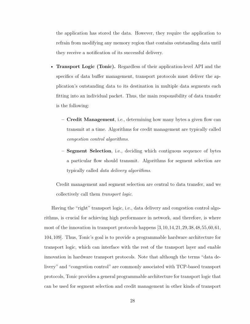
• Transport Logic (Tonic). Regardless of their application-level API and the

specifics of data buffer management, transport protocols must deliver the ap-

plication’s outstanding data to its destination in multiple data segments each

fitting into an individual packet. Thus, the main responsibility of data transfer

is the following:

– Credit Management, i.e., determining how many bytes a given flow can

transmit at a time. Algorithms for credit management are typically called

congestion control algorithms.

– Segment Selection, i.e., deciding which contiguous sequence of bytes

a particular flow should transmit. Algorithms for segment selection are

typically called data delivery algorithms.

Credit management and segment selection are central to data transfer, and we

collectively call them transport logic.

Having the “right” transport logic, i.e., data delivery and congestion control algo-

rithms, is crucial for achieving high performance in network, and therefore, is where

most of the innovation in transport protocols happens [3,10,14,21,29,38,48,55,60,61,

104,109]. Thus, Tonic’s goal is to provide a programmable hardware architecture for

transport logic, which can interface with the rest of the transport layer and enable

innovation in hardware transport protocols. Note that although the terms “data de-

livery” and “congestion control” are commonly associated with TCP-based transport

protocols, Tonic provides a general programmable architecture for transport logic that

can be used for segment selection and credit management in other kinds of transport

28

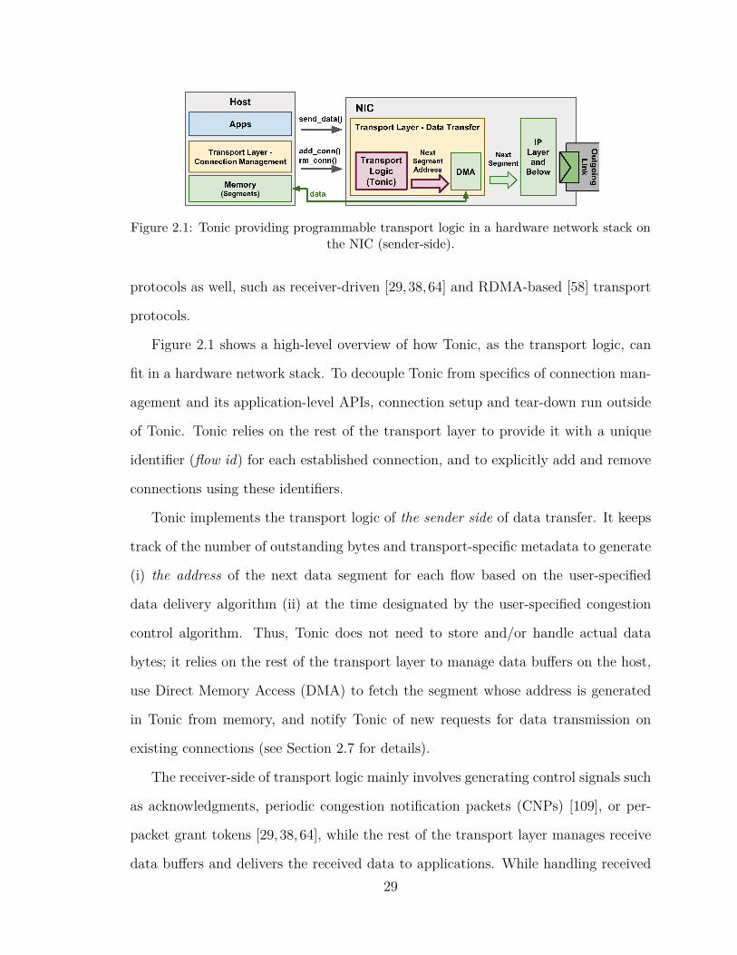
Figure 2.1: Tonic providing programmable transport logic in a hardware network stack onthe NIC (sender-side).

protocols as well, such as receiver-driven [29,38,64] and RDMA-based [58] transport

protocols.

Figure 2.1 shows a high-level overview of how Tonic, as the transport logic, can

fit in a hardware network stack. To decouple Tonic from specifics of connection man-

agement and its application-level APIs, connection setup and tear-down run outside

of Tonic. Tonic relies on the rest of the transport layer to provide it with a unique

identifier (flow id) for each established connection, and to explicitly add and remove

connections using these identifiers.

Tonic implements the transport logic of the sender side of data transfer. It keeps

track of the number of outstanding bytes and transport-specific metadata to generate

(i) the address of the next data segment for each flow based on the user-specified

data delivery algorithm (ii) at the time designated by the user-specified congestion

control algorithm. Thus, Tonic does not need to store and/or handle actual data

bytes; it relies on the rest of the transport layer to manage data buffers on the host,

use Direct Memory Access (DMA) to fetch the segment whose address is generated

in Tonic from memory, and notify Tonic of new requests for data transmission on

existing connections (see Section 2.7 for details).

The receiver-side of transport logic mainly involves generating control signals such

as acknowledgments, periodic congestion notification packets (CNPs) [109], or per-

packet grant tokens [29, 38, 64], while the rest of the transport layer manages receive

data buffers and delivers the received data to applications. While handling received29

data can get quite complicated due to out-of-order packet delivery, generating con-

trol signals on the receiver is typically simpler than the sender. Moreover, until very

recently [29, 38, 64], most of the innovation in transport protocols happened in the

sender side of transport logic. As a result, we mainly focus on providing programma-

bility for the sender side of transport logic. Reusing modules from the sender, we

have implemented a receiver solely for generating per-packet cumulative and selec-

tive acknowledgments and grant tokens at line rate. We leave the design of a more

programmable architecture for the receiver-side of transport logic to future work.

2.2 Hardware Design Challenges

Implementing transport logic at line rate in the NIC is challenging due to tight timing

and memory constraints.

Timing constraints. Data centers have a median packet size of less than 200

bytes [8, 84]. To achieve 100 Gbps for these small packets, the NIC has to send a

packet every ∼10 ns. Transport logic determines the address and transmission time

of the next data segment for each flow. Thus, every ∼10 ns, the transport logic should

output the address of the next available segment for transmission for one of several

active flows. However, it is challenging to do so since transport logic decisions require

stateful processing.

More specifically, to do credit management and segment selection, we need to

maintain state for each flow and update it on various transport-related events such as

segment generation, receipt of acknowledgements, and timeouts. This state is used

to decide which data segment should be transmitted next for that flow and at what

time. As a result, to generate back-to-back segments for the same flow, we must

quickly update the flow’s state after transport events. At the same time, updating a

flow’s state in response to transport events can involve complex operations depending

on the specific data delivery and congestion control algorithm in use.

30

We could conceivably pipeline the processing of transport events to “buy” more

time for performing complex operations. However, since processing back-to-back

events for the same flow requires updates to the same state, it would be difficult to

provide state consistency across the pipeline for events happening close to each other

in time. Thus, long pipelines cannot fully resolve this timing constraint. Instead,

we strive to process concurrent transport events within 10 ns, so that we can quickly

consolidate the state for the next event.

Memory constraints. A typical data-center server has more than a thousand

concurrent flows, each of which could have kilobytes of in-flight data [8,84,85]. Since

NICs have just a few megabytes of high-speed memory [52, 60], we can only store a

few kilobits of state per flow on the NIC for transport logic.

2.3 Common Patterns in Transport Logic

Tonic’s goal is to satisfy tight timing and memory constraints (Section 2.2) while

supporting programmability with a simple API. To do so, we identify common pat-

terns across transport logic in various protocols that we implement as reusable fixed-

function modules. These patterns allow us to optimize these modules for timing and

memory, while simplifying the programming API by reducing the functionality users

must specify. These patterns are summarized in Table 2.1, and are discussed in detail

in this section. Section 2.3.1 describes common patterns in segment selection, and

section 2.3.2 describes common patterns in credit management.

2.3.1 Segment Selection Patterns

With B bytes of credit, a flow can send S = max(B,MSS) bytes, where MSS is

the maximum segment size. Data-delivery algorithms, which are used for segment

selection, use acknowledgments to keep track of the status of each byte of data (e.g.,

31

# Pattern Examples1 Only track a limited window of segments TCP, NDP, IRN2 Only keep a few bits of state per segment TCP, NDP, IRN, RoCEv23 Lost segments first, new segments next TCP, NDP, IRN, RoCEv24 Loss detection: Acks and timeouts TCP, NDP, IRN

5 The three common credit calculation TCP, RoCEv2, NDPschemes: window, rate, and grant tokens

6 Congestion control parameter adjustment: TCP, Timely, DCQCNexternal and periodic internal signals

Table 2.1: Common transport logic patterns.

delivered, lost, in-flight, and not transmitted), and use that to decide which contigu-

ous S bytes of data to transmit next.

Note that with a few exceptions [58, 60], these algorithms are designed for soft-

ware, where they could store and freely loop through large arrays of metadata to

aggregate information. This computational flexibility has created significant diver-

sity across these algorithms. Unfortunately, NIC hardware is much more constrained

than software both in terms of computation and on-chip memory. Thus, we did not

aim to support all data-delivery algorithms. Instead, we looked for patterns that are

common across a variety of algorithms while being amenable to efficient hardware

implementation.

Moreover, due to memory constraints, the NIC, and consequently Tonic, cannot

store per-byte information. As a result, when describing segment selection patterns,

we assume that the data is already partitioned into fixed-size segments when the

flow requests transmission of new data, and that the segment selection decision hap-

pens based on per-segment, as opposed to per-byte, information (see section 2.4.2 for

details).

Pattern 1: Only Track a Limited Window of Segments

Independent of a flow’s available credit, data-delivery algorithms typically do not

transmit a new segment if it is too far from the first unacknowledged segment. In32

other words, if i is the ID of the first unacknowledged segment, no data segment with

an ID greater than i+ C is allowed to be transmitted, even if no other segments are

declared lost and the flow has enough credit for a new segment.

In TCP-based protocols, C is the minimum of receive window and congestion

window size. However, the limit imposed by C exists even when transport protocols

use other ways (e.g., rate) to limit a flow’s transmission pace and can be constant [58].

One rationale behind this is to limit the state that the receiver needs to keep in

case i is lost since the receiver would need to hold on to all the other segments before

it can hand them off to the application. This also implies that the sender only needs

to keep track of the status of a sliding window of at most C segments at a time,

bounding the amount of per-flow state that must be stored on the NIC. Thus, given

our tight memory constraints, this pattern helps limit the state that the sender (and

receiver) need to keep.

Pattern 2: Only Keep a Few Bits of State Per Segment

We observe that storing the following per-segment state is enough for implementing

most data-delivery algorithms:

• Is the segment acknowledged (in presence of selective acknowledgments)?

• If not, is it lost or still in flight?

• If lost, is it already retransmitted (to avoid redundant retransmission)?

More specifically, we observe that in the absence of explicit negative acknowledg-

ments, data-delivery algorithms accumulate evidence of loss for each segment from

positive acknowledgments, e.g., duplicate cumulative (e.g., TCP NewReno [37]) or

selective acknowledgments (e.g., IRN for RDMA and TCP SACK [10]). Once the

accumulated evidence of loss for a segment passes a threshold, the algorithm can

declare it lost with high confidence.33

Typically, an evidence of loss for segment i is also an evidence of loss for every

unacknowledged segment j with j < i. As a result, most of these algorithms can be

rewritten to only keep track of the total evidence of loss for the first unacknowledged

segment and incrementally compute the evidence for the rest as needed using the

per-segment information listed above.

This pattern helps with our tight memory constraints as well. Although not as

expensive as per-byte state, keeping per-segment state can be costly as well. In a 100

Gbps network with a 10µs RTT, a flow can have as many as ∼128 segments in flight.

Thus, being able to only keep a few bits of state per segment helps us stay within the

NIC’s memory limits while supporting a wide range of data delivery algorithms.

Moreover, except for the bit that keeps track of whether a segment is lost, updating

the rest is similar across data delivery algorithms and therefore can be implemented

as a fixed-function module. As we discuss in section 2.4.2, these updates involve

bitmap operations that are difficult to implement efficiently at high speed. Thus, this

observation helps with reducing the development effort of Tonic’s users as well.

Pattern 3: Lost Segments First, New Segments Next

If a data-delivery algorithm infers that a segment is lost, it is only logical to retransmit

it before transmitting anything new as the receiving application cannot use the new

segments of that flow without first receiving the lost one. As a result, although dif-

ferent algorithms have different ways of inferring segment loss, once the lost segments

are detected, the procedure for selecting the next segment is the same irrespective of

the specific data-delivery algorithm in use.

Based on this pattern, we can implement segment address generation logic as

a fixed function module in Tonic. As a result, we can optimize it for timing and

memory, while reducing the functionality users must specify.

34

Pattern 4: Loss Detection: Two Mutually-Exclusive Signals

To determine lost segments, data delivery algorithms keep state variables (per-flow

and per-segment) and update them when they receive new information: either in the

form of a new acknowledgment from the receiver, or the absence of acknowledgments

for a period of time (timeout).

This helps us in two ways. First, it limits the modules for segment selection that

require user specification to two for processing these two signals, namely acknowl-

edgments and timeouts. Second, since the two signals are, by definition, mutually

exclusive, they never need to update the flow’s state at the same time, thus limiting

the number of concurrent updates to per-flow state for loss detection and simplifying

Tonic’s architecture (see section 2.4.2 for details).

2.3.2 Credit Management Patterns

Transport protocols use congestion-control algorithms to do credit management, i.e.,

to avoid overloading the network by controlling the pace of a flow’s transmission.

These algorithms consist of a control loop that estimates the network capacity by

monitoring the stream of incoming control packets (e.g., acknowledgments and con-

gestion notification packets (CNPs)) and sets parameters that limit outgoing data

packets. Our main observation, detailed below, is that while the control loop that

adjusts credit management parameters is different in many algorithms, credit calcu-

lation based on those parameters is not.

Pattern 5: The Three Common Credit-Calculation Schemes

Congestion control algorithms have a broad range of ways to estimate network ca-

pacity. However, they enforce limits on data transmission in three main ways:

35

• Congestion window. The control loop limits a flow to at most W bytes in

flight from the first unacknowledged byte. Thus, if byte i is the first unacknowl-

edged byte, the flow cannot send bytes beyond i+W .

• Rate. The control loop limits the flow’s average rate (R) and maximum burst

size (D). Thus, if a flow had credit c0 at the time t0 of the last transmission,

then the credit at time t will be min(R ∗ (t− t0) + c0, D).

• Grant tokens. Instead of estimating network capacity, the control loop re-

ceives tokens from the receiver and adds them to the flow’s credit. Thus, the

credit of a flow is the total tokens received minus the number of transmitted

bytes, and the credit calculation logic consists of a simple addition.

While credit calculation for explicit tokens consists of a simple addition, enforcing

congestion window and rate can become complicated. For instance, keeping track of

in-flight segments to enforce a congestion window is challenging in the presence of se-

lective acknowledgements, and so is implementing precise per-flow rate limiters under

out tight timing and memory constraints. This observation allows us to implement

these three credit calculation schemes as fixed-function modules and optimize their

implementation to meet out timing and memory constraints.

Pattern 6: Parameter Adjustment: External and Periodic Internal Signals

Control loops often continuously monitor the network and adjust credit calculation

parameters, i.e., rate or window size, based on estimated network capacity. We

observe that parameter adjustment is triggered by the following groups of signals:

• External Signals. Some parameter adjustments are triggered by external sig-

nals received in incoming packets. A common example is acknowledgments.

Acknowledgments are used in data delivery algorithms to detect packet loss.

36

However, some congestion control algorithms use packet loss as well to re-

duce congestion control parameters (e.g., window adjustment after duplicate

acknowledgments in TCP). Moreover, acknowledgments can carry other signals

such as Explicit Congestion Notification (ECN) bits, which are used in some

TCP variants for congestion window adjustment (e.g., DCTCP). Acknowledg-

ments can also be used to calculate round trip times (RTTs), i.e., delay, and use

that for parameter adjustment (e.g., Timely). Finally, external signals could

be in forms other than acknowledgments. DCQCN, for instance, uses conges-

tion notification packets (CNPs) generated at the receiver to adjust a flow’s

transmission rate.

• Periodic Internal Signals. Several control loops use internal per-flow timers

and counters to periodically adjust congestion control parameters. For instance,

many data delivery algorithms use retransmission timers to retransmit unac-

knowledged segments if no acknowledgment is received within a certain period

of time. The same timer is used in some congestion control algorithms (e.g.,

TCP variants) to perform parameter adjustment. As another example, DCQCN

uses a byte counter and various periodic timers to adjust the transmission rate

of each flow.

Control loop logic for parameter adjustment varies among congestion control al-

gorithms, and so needs to be programmable by users. This pattern, similar to pattern

#4, helps us limit the modules for credit management that require user specification

to two, one for processing incoming packets for external signals, and one for checking

and processing periodic internal signals. Moreover, the triggers for the two pro-

grammable modules for segment selection (see pattern #4) align with those for credit

management, thus helping us simplify Tonic’s architecture and its programming API.

37

Figure 2.2: Tonic’s architecture (red boxes (also with thick borders) are programmable,others are fixed)

2.4 Tonic Architecture

Tonic exploits the natural functional separation between segment selection and credit

management to partition them into two components with separate state (Figure 2.2).

The segment selection engine processes events related to generating, tracking, and

delivery of segments, while the credit engine processes events related to adjusting

each flow’s credit and sending out segments addresses for those with sufficient credit.

At the cost of lightweight coordination between the two engines, this partitioning

helps Tonic meet its timing constraints while concurrently processing multiple events

(e.g., receipt of acknowledgments and segment transmission) every cycle. These events

must read the current state of their corresponding flow, update it, and write it back to

memory for events in the next cycle. However, concurrent read and write to memory

in every cycle is costly. Instead of using a wide memory to serve all the transport

events, the partitioning allows the segment selection engine and credit engines to have

narrower memories to serve only the events that matter for their specific functionality,

hence meeting timing constraints.

In this section, we first present how the two engines coordinate to fairly and effi-

ciently pick one of thousand flows every cycle for segment transmission while keeping

the outgoing link utilized (section 2.4.1). Next, section 2.4.2 and section 2.4.3 describe

38

fixed-function and programmable event processing modules in each engine, and how

their design is inspired by patterns in section 2.3, using TCP-based, receiver-driven,

and RDMA-based protocols as examples. Finally, we present Tonic’s solution for

resolving conflicts when more than one event for the same flow is received in a cycle

in section 2.4.4.

2.4.1 Efficient Flow Scheduling

At any time, a flow can only transmit a data segment if it (1) has enough credit,

and (2) has a new or lost segment to send. To be work conserving, Tonic must track

the set of flows that are eligible for transmission (meet both of the above criteria)

and only pick among those when selecting a flow for transmission each cycle. This

is challenging to do efficiently. We have more than a thousand flows with their state

partitioned across two engines: Only the credit engine knows how much credit a flow

has, and only the segment selection engine knows the status of a flow’s segments and

can generate the address of its next segment. We cannot check the state of all the

flows every cycle across both engines to find the ones eligible for transmission in that

cycle.

Instead, we decouple the generation of segment addresses from their final trans-

mission to the DMA pipeline. We allow the segment selection engine to generate up

to N segment addresses for a flow without necessarily having enough credit to send

them out. In the credit engine, we keep a ring buffer of size N for each flow to store

these outstanding segments addresses. When the flow has enough credit to send a

segment, the credit engine dequeues and outputs a segment address from the buffer

and signals the segment selection engine to decrement the number of outstanding

segments for that flow.

This solves the problem of the partitioned state across the two engines. The

segment selection engine does not need to keep track of the credit changes of flows

39

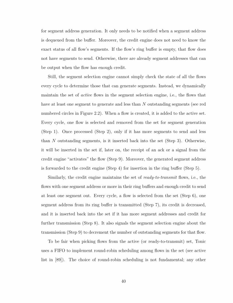
for segment address generation. It only needs to be notified when a segment address

is dequeued from the buffer. Moreover, the credit engine does not need to know the

exact status of all flow’s segments. If the flow’s ring buffer is empty, that flow does

not have segments to send. Otherwise, there are already segment addresses that can

be output when the flow has enough credit.

Still, the segment selection engine cannot simply check the state of all the flows

every cycle to determine those that can generate segments. Instead, we dynamically

maintain the set of active flows in the segment selection engine, i.e., the flows that

have at least one segment to generate and less than N outstanding segments (see red

numbered circles in Figure 2.2). When a flow is created, it is added to the active set.

Every cycle, one flow is selected and removed from the set for segment generation

(Step 1). Once processed (Step 2), only if it has more segments to send and less

than N outstanding segments, is it inserted back into the set (Step 3). Otherwise,

it will be inserted in the set if, later on, the receipt of an ack or a signal from the

credit engine “activates” the flow (Step 9). Moreover, the generated segment address

is forwarded to the credit engine (Step 4) for insertion in the ring buffer (Step 5).

Similarly, the credit engine maintains the set of ready-to-transmit flows, i.e., the

flows with one segment address or more in their ring buffers and enough credit to send

at least one segment out. Every cycle, a flow is selected from the set (Step 6), one

segment address from its ring buffer is transmitted (Step 7), its credit is decreased,

and it is inserted back into the set if it has more segment addresses and credit for

further transmission (Step 8). It also signals the segment selection engine about the

transmission (Step 9) to decrement the number of outstanding segments for that flow.

To be fair when picking flows from the active (or ready-to-transmit) set, Tonic

uses a FIFO to implement round-robin scheduling among flows in the set (see active

list in [89]). The choice of round-robin scheduling is not fundamental; any other

40

scheduler that meets our timing constraints can replace the FIFO to support other

scheduling disciplines [91].

2.4.2 Flexible Segment Selection

Tonic’s segment selection engine decides which contiguous sequence of bytes from a

flow’s outstanding data to transmit next. As such, it needs to process events related

to generating and tracking the delivery status of segments and update each flow’s

state accordingly. Every cycle, the segment selection engine selects a flow from the

set of active flows and, based on the flow’s state, generates its next segment address.

The segment address, along with its corresponding flow id, is forwarded to the credit

engine for queueing and final transmission.

In transport protocols, data delivery algorithms are used for segment selection. To

enable Tonic’s users to implement and modify data delivery algorithms with modest

development effort, we use the observed patterns in section 2.3 to provide (i) optimized

fixed-function modules that can be reused across several algorithms, and (ii) the

minimal set of programmable modules required to support a wide range of algorithms.

Pre-Calculated Fixed Segment Boundaries

With B bytes of credit, a flow can send S = max(B,MSS) bytes, where MSS is

the maximum segment size. Data-delivery algorithms could conceivably choose the

next S bytes to send from anywhere in the data stream and produce segments with

variable boundaries. However, since the NIC cannot maintain per-byte state, Tonic

requires data to be partitioned into fixed-size segments (by a Kernel module or the

driver, see section 2.7) when the flow requests transmission of new data. This way,

data-delivery algorithms can use per-segment information to select the next segment.

With message-based transport protocols (e.g., RoCEv2), having fixed segment

boundaries fits naturally; the message length is known from the beginning and can

41

be optimally partitioned into segments. For transport protocols that provide a byte-

stream abstraction (e.g., TCP and NDP), having fixed segment boundaries does not

affect the throughput of high-bandwidth flows as their data can be partitioned into

MSS-sized segments. For flows that generate small data segments and sporadically,

there is a possibility of creating many small segments, and they benefit less from

Tonic (see section 2.7.1). Regardless, due to memory constraints, segmentation is

done outside of Tonic and does not affect high-bandwidth flows.

Concurrent Event Processing

For every flow, four main events can affect the generation of its next segment address:

• Acknowledgment. The receipt of an acknowledgment can either move the

window forward and enable the flow to generate more segments, or signal seg-

ment loss and trigger retransmissions.

• Timeout. The absence of acknowledgments, i.e., a timeout, can also lead to

more segments marked as lost and trigger retransmissions.

• Segment Generation. Once a segment is generated, it will be forwarded to the

credit engine to wait in the queue for outstanding segments. Thus, Generation

of a segment address increments the number of a flow’s outstanding segments

and can deactivate the flow if it goes over N .

• Segment Transmission. Segment address transmission (out of the credit

engine) decrements the number of outstanding segments and can enable the

flow to generate more segment addresses.

Tonic’s segment selection engine has four modules to handle these four events

(Figure 2.2). Every cycle, each module reads the state of the flow for which it received

an event from the memory in the segment selection engine, processes the event, and

updates the flow state accordingly.42

The flow state in the segment selection engine consists of a fixed set of variables

to track the status of the current window of segments across events, as well as the

user-defined variables used in the programmable components. For instance, we use

patterns #1 and #2 (section 2.3.1) to only keep a fixed set of bitmaps for each flow

to track the status of its segments. The acked bitmap keeps track of selectively

acknowledged segments, marked-for-rtx keeps track of lost segments that require

retransmission, and rtx-cnt stores information about their previous retransmissions.

As another example, we track the first unacknowledged segment and the highest

generated segment ID for each flow as well. The full list of the fixed state variables

for each flow is presented in Table 2.2.

The following paragraphs describe how each event-processing module affects a

flow’s state, and which patterns we used in their design. For programmable modules,

the detailed API is covered in section 2.5.

Incoming. This module processes acknowledgments for segment selection. Based

on patterns #1 and #2 (section 2.3.1), some updates to state variables in response to

acknowledgments are similar across all data-delivery algorithms and do not need to

be programmable (e.g., updating window boundaries, and marking selectively acked

segments in acked bitmap). On the other hand, loss detection and recovery, which

rely on acknowledgments as a signal, vary a lot across different algorithms and must

be programmable by users (pattern #4, section 2.3.1). Thus, the Incoming module

is designed as a two-stage pipeline: a fixed-function stage for the common updates

followed by a programmable stage for loss detection and recovery.

The benefit of this two-stage design is that the common updates mostly involve

bitmaps and arrays, which are implemented as ring buffers in hardware and costly

to modify across their elements. For instance, in all data delivery algorithms, if an

incoming packet acknowledges segment C cumulatively and segment S selectively,

wnd-start is updated to max(wnd-start, C) and acked[S] to one, and the boundaries

43

State Variable Descriptionacked selectively acknowledged segments (bitmap)marked-for-rtx lost segments marked for retransmission (bitmap)rtx-cnt number of retransmissions of a segment (bitmap)wnd-start the address of the first segment in the windowwnd-size size of the window (min(W, rcved_window))highest-sent the highest segment transmitted so fartotal-sent Total number of segments transmitted so faris-idle does the flow have segments to send?outstanding-cnt # of outstanding segmentsrtx-timer when will the rtx timer expire?user-context user-defined variables for programmable modules

Table 2.2: Per-flow state variables in the segment selection engine

of all bitmaps and arrays are updated based on the new wnd-start. By moving

these updates into a fixed function stage, we can (i) optimize them to meet Tonic’s

timing and memory constraints, and (ii) provide the programmers with a dedicated

stage, i.e., a separate cycle, to do loss detection and recovery, where they can use

the updated state variables from the previous stage, the rest of the variables from

memory to infer segment loss.

The incoming module is used for processing incoming packets other than acknowl-

edgments as well. Per pattern #6 (section 2.3.2), congestion control loops depend on

external signals, not necessarily in form of acknowledgments, to perform parameter

adjustment. Moreover, the parameter adjustment logic in response to signals varies

significantly among different congestion control algorithms, and therefore, needs to

be programmable. Additionally, many control loops (e.g., TCP variants) rely on seg-

ment loss for parameter adjustment. Thus, while credit calculation is done in the

credit engine, the user-defined logic for parameter adjustment in response to external

signals is performed in the programmable stage of the incoming module. The updated

parameters are then forwarded to the credit engine for enforcement.

Periodic Updates. This module processes timeouts. The segment selection

engine iterates over the active flows, sending them one at a time to this module to

check for retransmission timer expiration. Thus, with its 10 ns clock cycle, Tonic

44

can cover each flow within a few microseconds of the expiry of its retransmission

timer. This module must be programmable as a retransmission timeout is a signal

for detecting loss (pattern #4, section 2.3.1). Similar to the programmable stage

of the Incoming module, the programmers can use per-flow state variables to infer

segment loss.

Similar to the programmable stage of the Incoming module, the Periodic Updates

module is used for periodic events other than a retransmission timer. Per pattern #6

(section 2.3.2), congestion control loops depend on periodic internal signals, such as

counters and timers in DCQCN, to do parameter adjustment. As a result, the user-

defined periodic internal signals and the logic for parameter adjustment in response

to them is also performed in the Periodic Updates module in the segment selection

engine. Similar to the parameter adjustment in the Incoming module, the updated

parameters are then forwarded to the credit engine for enforcement.

Segment Generation. Given an active flow and its variables, this module gen-

erates the next segment’s address and forwards it to the credit engine. Tonic can

implement segment address generation as a fixed function module based pattern #3

in section 2.3.1: once a lost segment is detected, it is only logical to retransmit it before

sending anything new. Thus, this module prioritizes retransmission of lost segments

in marked-for-rtx over sending the next new segment, i.e., highest_sent+1. It also

increments the number of outstanding segments to deactivate the flow if it has more

than N outstanding segments.

Segment Transmitted. This module is fixed function and is triggered when a

segment address is transmitted out of the credit engine. It decrements the number of

outstanding segments of the corresponding flow. If the flow was deactivated due to a

full ring buffer, it is inserted into the active set again.

45

2.4.3 Flexible Credit Management

The credit engine keeps track of each flow’s credit and sends out segment addresses

for those with sufficient credit. A flow’s credit is determined by the congestion control

algorithm in use. These algorithms typically consist of a control loop that estimates

the network capacity and adjusts congestion control parameters that limit outgoing

data segments.

As discussed in section 2.3.2, while the control loop logic for adjusting parameters

is different in many algorithms, there are only three main ways in which these param-

eters are enforced: congestion window, rate, and grant tokens (Pattern #5). Conges-

tion window calculations are mostly affected by acknowledgments, Thus, calculation

and enforcement of congestion window happens in the segment selection engine. For

the other two credit calculation schemes, Tonic relies on the credit engine to process

credit-related event, and Tonic users can simply pick which credit-calculation scheme

to use in the credit engine.

Parameter adjustment logic in response to external and periodic internal signals

(pattern #6) vary across various congestion control algorithms and need to be pro-

grammable by the user. As discussed in section 2.4.2, parameter adjustment logic is

implemented in the programmable modules of segment selection engine, but the up-

dated parameters are forwarded to the credit engine to be used for credit calculation.

To summarize, Tonic’s credit engine performs credit calculations and credit en-

forcement for rate and grant tokens, and leaves the enforcement of congestion window

and congestion control parameter adjustment to the segment selection engine due to

architectural overlaps. Thus, the rest of this section describes the concurrent event

processing that occurs in the credit engine for enforcing rate and grant tokens.

46

Concurrent Event Processing for Credit Calculation

Conceptually, three main events can trigger credit calculation for a flow, and the credit

engine has different modules to concurrently process them every cycle (Figure 2.2):

• Enqueue Segment. When a segment address is received from the segment

selection engine and is the only one in the flow’s ring buffer, the flow could now

qualify for transmission or remain idle based on its credit.

• Transmit Segment. When a flow transmits a segment address, its credit

must be decreased and we should determine whether it is qualified for further

transmission based on its updated credit and the occupancy of its ring buffer

• Add Credit. Some events result in adding credit to the flow (e.g., from grant

tokens and leaky bucket rate limiters). This is where the main difference lies

between rate-based and token-based credit calculation and is described in more

detail below.

When using grant tokens, the credit engine needs two dedicated modules to add

credit to a flow: one to process incoming grant tokens from the receiver, and one to

add credit on timeouts in case it is needed for retransmissions. When using rate, the

credit engine does not need any extra modules for adding credit since a flow with rate

R bytes-per-cycle implicitly gains R bytes of credit every cycle and, therefore, we can

compute in advance when it will be qualified for transmission.

Suppose in cycle T0, the Transmit module transmits a segment from flow f , and

is determining whether the flow is qualified for further transmission. Suppose that

f has more segments in the ring buffer but lacks C bytes of credit. The Transmit

module can compute when it will have sufficient credit as T = CRand set up a timer

for T cycles. When the timer expires, f definitely has enough credit for at least

one segment, so it can be directly inserted into ready-to-tx. When f reaches the

47

head of ready-to-tx and is processed by the Transmit module again in cycle T1, the

Transmit module can increase f ’s credit by (T1 − T0) ∗R− S, where S is the size of

the segment that is transmitted at time T1. Similarly, the Enqueue module can set up

the timer when it receives the first segment of the queue and the flow lacks credit for

its transmission. Note that when using rate, the credit engine must perform division

and maintain per-flow timers. We will discuss the hardware implementation of these

operations in section 2.6.1.

2.4.4 Handling Conflicting Events

Tonic strives to process events concurrently in order to be responsive to events. Thus,

if a flow receives more than one event in the same cycle, it allows the event processing

modules to process the events and update the flow’s state variables, and reconciles

the state before writing it back into memory (the Merge modules in Figure 2.2).

Since acknowledgments and retransmission timeouts are, by definition, mutually

exclusive (Pattern #4, section 2.3.1), Tonic discards the timeout if it is received in the

same cycle as an acknowledgment for the same flow. This significantly simplifies the

merge logic because several variables (window size and retransmission timer period)

are only modified by these two events and, therefore, will never be concurrently

updated. We can resolve concurrent updates for the remaining variables with simple,

predefined merge logic. For example, Segment Generation increments the number of

outstanding segments, whereas Segment Transmitted decrements it; if both events

affect the same flow at the same time, the number does not change. User-defined

variables are updated in either the Incoming or the Periodic Updates module, and

we rely on the user to specify which updated variables should be prioritized if both

updates happen in the same cycle.

48

2.5 Tonic’s Programming Interface

To implement a new transport logic in Tonic, programmers only need to specify the

following: (i) the credit management scheme, i.e., one of congestion window, rate, or

grant tokens. (ii) the loss detection and recovery logic in response to acknowledgments

and timeouts, and (iii) congestion-control parameter adjustment in response to in-

coming packets or periodic timers and counters. The first one is used to pick the right

modules for the credit engine, and the last two are inserted into the corresponding

programmable stages of the segment selection engine (Figure 2.2).

To specify the logic for the programmable stage of the Incoming module, pro-

grammers need to write a function that receives the incoming packet (acknowledg-

ment or other control signals), the number of newly acknowledged segments, the

acked bitmap updated with the information in the acknowledgment, the old and new

value of wnd-start (in case the window moves forward due to a new cumulative ac-

knowledgment), and the rest of the flow’s state variables (Table 2.2) as input. In

the output, they can mark a range of segments for retransmission in marked-for-rtx,

update congestion-control parameters such as window size and rate, and reset the

retransmission timer. The programming interface of the Periodic Updates module is

similar.

In specifying these functions, programmers can use integer arithmetic operations,

e.g., addition, subtraction, multiplication, and division with small-width operands,

conditionals, and a limited set of read-only bitmap operations, e.g., index lookup,

and finding the first set bit in the updated acked bitmap 2.

As we show in section 2.8.1, these operations are sufficient for implementing several

data delivery and congestion control algorithms. We implemented those with inte-

ger arithmetic operations without any modifications. For those with floating point2Note that, as we described in section 2.4.2, a dedicated fixed-function stage in the data delivery engineperforms the costly common bitmap updates on receipt of acknowledgments. That’s why the bitmapoperations in programmable modules are limited and read-only.

49

operations, such as DCQCN, we approximated the operations to a certain decimal

point using integer operations. If an algorithm requires high-precision and compli-

cated floating point operations that cannot be implemented within one clock cycle

(e.g., a subset of rate calculations in PCC [21]), the computation can be relegated

to a floating-point arithmetic module outside of Tonic. This module can perform

the computation asynchronously and store the output in a separate memory, which

periodically merges into Tonic through the “Periodic Updates” module.

2.6 Hardware Implementation

In this section, we describe the hardware design of the Tonic components that were the

most challenging to implement under Tonic’s tight timing and memory constraints.

2.6.1 High-Precision Per-Flow Rate Limiting

When using rate in the credit engine, if a flow with rate R bytes per cycle needs

C more bytes of credit to transmit a segment, Tonic calculates T = dCRe as the

time where the flow will have sufficient credit for transmission. It sets up a timer

that expires in T cycles, and upon its expiry, queues up the flow in ready-to-tx for

transmission (section 2.4.3). Note that T must be calculated in the fast path. Since

we cannot afford to do floating-point division in the fast path, R must be represented

as an integer.

This creates a trade-off between the rate-limiting precision and the range of rates

Tonic can support. If we represent R in bytes per cycle, we can compute the exact

cycle when the flow will have enough credit but cannot support rates lower than one

byte per cycle or ∼1 Gbps. If we instead represent R in, say, bytes per thousand

cycles, we can support lower rates (e.g., 1 Mbps), but T = dCRe will determine how

many thousand cycles from now the flow can qualify for transmission. This results

in lower rate conformance and precision for higher-bandwidth flows. As a concrete

50

example, for a 20 Gbps flow, R would be 25000 bytes per thousand cycles. Suppose

the flow has a 1500-byte segment to transmit. It will have enough credit to do so in

8 cycles but has to wait d 150025000e = 1 thousand cycles to be queued for transmission.

Instead of committing to one representation for R, Tonic keeps multiple state

variables R1, . . . , Rk for each flow, each representing the flow’s rate at a different level

of precision. As the congestion control loop adjusts the rate according to the network

capacity, Tonic can switch between R1, . . . , Rk to pick the most precise representation

for computing T at any moment. This enables Tonic to support a wide range of per-

flow rates, from ∼1.5Mbps to 100Gbps at 1.5Mbps granularity, without sacrificing

the rate-limiting precision.

2.6.2 Efficient Bitmap Operations

Tonic uses bitmaps as large as 128 bits to track the status of a window of segments

for each flow. Bitmaps are implemented as ring buffers, with the head pointer cor-

responding to the first unacknowledged segment. As new acknowledgments arrive,

the head pointer moves forward around the ring. To efficiently implement operations

whose output depends on the values of all the bits in the bitmap, we must parallelize

them by dividing the ring buffer into smaller parts, processing them in parallel, and

joining the results. For large ring buffers, this divide and conquer pattern is repeated

in multiple layers. As each layer depends on the previous one for its input, we must

keep the computation in each layer minimal to stay within our 10 ns target.

One such operation finds the first set bit after the head. This operation is used

to find the next lost segment for retransmission in the marked-for-rtx bitmap. The

moving head of the ring buffer complicates the implementation of this operation.

Suppose we have a 32-bit ring buffer A32, with bits 5 and 30 set to one, and the

head at index 6. Thus, findfirst(A32, 6) = 30. We divide the ring into eight four-bit

parts, “or” the bits in each one, and feed the results into an 8-bit ring buffer A8,

51

where A8[i] = OR(A32[i : i+ 3]). So, only A8[1] and A8[7] are set. However, because

the set bit in A32[4 : 7] is before the head in the original ring buffer, we cannot simply

use one as A8’s head index or we will mistakenly generate 5 instead of 30 as the final

result. So, we need extra computation to find the correct new head. For a larger ring

buffer with multiple layers of this divide and conquer pattern, we need to compute

the head in each layer.

Instead, we use a lightweight pre-processing on the input ring buffer to avoid head

index computation altogether. More specifically, using A32 as input, we compute

A′32 which is equal to A32 except that all the bits from index zero to head (6 in our

example) are set to zero. Starting from index zero, the first set bit in A′32 is always

closer to the original head than the first set bit in A32. So, findfirst(A32, 6) equals

findfirst(A′32, 0) if A′

32 has any set bits, and otherwise findfirst(A32, 0). This way,

independent of the input head index H, we can always solve findfirst(A,H) from

two subproblems with the head index fixed at zero.

2.6.3 Concurrent Memory Reads and Writes

The memory in the segment selection engine is concurrently accessed by five modules

(including both stages of the Incoming module) every cycle (section 2.4.2). However,

FPGAs only have dual-ported block RAMs (BRAMs), with each port capable of

either read or write every cycle. To build a memory with, say, two read and two write

ports, we can use two BRAMs, or “banks”, to store two copies of the data, but only

update one on each write [47]. Using a table to keep track of the bank with the most

recent data for each address, we can support two concurrent reads and writes with

the four ports of the two BRAMS.

Supporting more concurrent reads and writes would require even more replication

of state 3. To avoid supporting five concurrent reads and writes, we managed to3This overhead is specific to FPGAs, and can potentially be eliminated if the memory is designed as anASIC.

52

partition the per-flow state variables into two groups each affected by at most four

different events. As a result, Tonic can use two memories with four read and four

write ports instead of a single one with five read and write ports, providing concurrent

access for all processing modules in the segment selection engine at the same time.

2.7 Integrating Tonic into the Transport Layer

This section provides two examples of how to integrate Tonic into the commonly-used

transport layers: Linux kernel with sockets as the application level API (section 2.7.1),

and RDMA-based transport using Verbs API (section 2.7.2).

2.7.1 Linux Kernel and Socket API

After creating and configuring the socket, the application uses multiple system calls

for connection management and data transfer. Note that as discussed in section 2.1,

Tonic mainly focuses on the sender sider of the transport logic. Thus, we only discuss

the system calls and modifications relevant to the sender side of the transport layer.

Connection Management. These system calls include connect() on the client

to initiate a connection, listen() and accept() on the server to listen for and accept

new connections, and close() to terminate a connection. Since connection man-

agement happens outside of Tonic, the kernel implementation of these system calls

stays untouched. However, once the connection is established, the kernel maps it to

a unique flow id in [0, N), where N is the maximum number of flows supported by

Tonic. The kernel then notifies Tonic through the NIC driver about the new con-

nection. Specifically, from the Transmission Control Block (TCB) allocated for the

connection in the kernel, the IP addresses and ports of the communication endpoints

and the maximum segment size (MSS) should be sent to Tonic alongside the flow id.

Note that for flows using Tonic for data transfer, the kernel only needs to track

those fields in the TCB that are for connection management (e.g., IP addresses,

53

ports, and TCP connection finite state machine (FSM)), pointers to data buffers,

and receiver-related fields. Fields used for data transfer for the sender, i.e., snd.nxt,

snd.una, and snd.wnd, are stored in and handled by Tonic. Finally, after a call to

close(), the kernel notifies Tonic of connection termination using the connection’s

flow id.

Data Transfer. At a high level, send() adds more data to the connection’s

socket buffer, which stores the connection’s outstanding data waiting for delivery. As

discussed in section 2.4.2, Tonic keeps per-segment state for outstanding data and

performs all transport logic computation in terms of segments. Therefore, data needs

to be partitioned into equal-sized segments before Tonic can start its transmission.

As a result, the modifications to the implementation of send() mainly involve deter-

mining segment boundaries for the data in the socket buffer and deciding when to

notify Tonic of the existence of new data segments.

More specifically, the kernel keeps an extra pointer for each connection’s socket

buffer, in addition to its head and tail, called tonic-tail. It points to the end of the

last data segment of which Tonic has been notified and is used in the segmentation

process described below. head and updates to tonic-tail are sent to Tonic to use

when generating the address of the next segment to fetch from memory.

Starting with an empty socket buffer, when the application calls send(), data

is copied to the socket buffer, and tail is updated accordingly. The data is then

partitioned into MSS-sized segments. Suppose the data is partitioned into S segments

and B < MSS remaining bytes. The kernel then updates tonic-tail to point to

the end of the last MSS-sized segment, i.e., head + MSS * S, and notifies Tonic of the

update to tonic-tail. The extra B bytes remain unknown to Tonic for a configurable

time T , in case the application calls send to provide more data. In that case, the

data are added to the socket buffer, data between tonic-tail and tail are similarly

54

partitioned, tonic-tail is updated accordingly, and Tonic is notified of new data

segments.

If there is not enough data for a MSS-sized segment after T , the kernel needs to

notify Tonic of the “small” segment and its size, and update tonic-tail accordingly.

Note that Tonic requires all segments, except for the last one in a burst, to be of equal

size, as all computations, including window updates, are in terms of segments. Thus,

after creating a “small” segment, if there is more data from the application, Tonic can

only start its transmission when it is done transferring its current segments. Tonic

notifies the kernel once it successfully delivers the final “small” segment, at which

point, head and tonic-tail will be equal, and the kernel continues partitioning the

remaining data in the socket buffer and updating Tonic as before. Note that Tonic

can periodically forward acknowledgements to the kernel to move head forward and

free up space for new data in the socket buffer.

Other Considerations. As we show in section 2.8, Tonic’s current design sup-

ports 2048 concurrent flows, which matches the working sets observed in data cen-

ters [8,84] and other hardware offloads in the literature [24]. If a host has more open

connections than Tonic can support, the kernel can offload data transfer for high-

bandwidth flows to Tonic on a first-come first-serve basis, or have users set a flag

when creating the socket and fall back to software once Tonic runs out of resources

for new flows. Alternatively, modern FPGA-based NICs have a large DRAM directly

attached to the FPGA [24]. The DRAM can potentially be used to store the state of

more connections, and swap them back and forth into Tonic’s memory as they acti-

vate and need to transmit data. Moreover, to provide visibility into the performance

of hardware transport logic, Tonic can provide an interface for kernel to periodically

pull transport statistics from the NIC.

Takeaways. Linux kernel can be modified so applications can use Tonic through

the socket API. That said, Tonic is most beneficial for high-bandwidth flows that

55

generate MSS-sized segments. Flows that sporadically generate small segments do

not benefit as much, as small segments cannot be consolidated within Tonic. We

emphasize that the above design serves as an example of how Tonic can be integrated

into a commonly-used transport layer. However, TCP, sockets, and byte streams are

not always suitable for high-bandwidth, low-latency flows. In fact, several such data-

center applications are starting to use RDMA and its message-based API instead [34,

61, 72, 82]. Tonic can be integrated into RDMA-based transport as well, which we

discuss next.

2.7.2 RDMA NICs and Verbs API

Remote Direct Memory Access (RDMA) enables applications to directly access mem-

ory on remote endpoints without involving the CPU. To do so, the endpoints create

a queue pair, analogous to a connection, and post requests, called Work Queue Ele-

ments (WQEs), for sending or receiving data from each other’s memory. Although

RDMA originated from InfiniBand networks, RDMA over Ethernet is getting more

common in data centers [34,61,82]. In the rest of this section, we use RDMA to refer

to RDMA implementations over Ethernet.

Once a queue pair is created, RDMA NICs can add the new “connection” to Tonic

and use it to on the sender side to transfer data in response to different WQEs. Each

WQE corresponds to a separate message transfer and therefore nicely fits Tonic’s

need for partitioning data into segments before starting transmission.

For instance, in an RDMA Write, one endpoint posts a Request WQE to write to

memory on the other endpoint. Data length, data source address on the sender, and

data sink addresses on the receiver are specified in the Request WQE. Thus, a shim

layer between RDMA applications and Tonic can break the data into segments and

notify Tonic of number of segments, and the source memory address to read the data

56

from on the sender. Once Tonic generates the next segment address, the rest of the

RDMA NIC should DMA it from the sender’s memory and add appropriate headers.

An RDMA Send is similar to RDMA Write, except it requires a Receive WQE on

the receiver to specify the sink address to which the data from the sender should be

written. So, the sender side can still use Tonic in the same way. As another example,

in an RDMA Read, one endpoint requests data from memory on the other endpoint.

So, the responder endpoint should transmit data to the requester endpoint. Again,

the data length, data source on the responder, and data sink on the requester are

specified in the WQE, and the shim layer can break it into segments and transfer it

using Tonic.

Thus, Tonic can be integrated into RDMA NICs to replace the hard-coded trans-

port logic on the sender-side of data transfer. In fact, two of our benchmark protocols,

RoCE with DCQCN [109] and IRN [60] are proposed for RDMA NICs. That said,

this is assuming we have a compatible receiver on the other receiver-side to generate

the control signals (e.g., acknowledgements, congestion notifications, etc.) required

by whichever transport protocol one chooses to implement on Tonic on the sender

side.

While some implementations of RDMA over Ethernet such as iWarp [16] handle

out-of-order (OOO) packets and implement TCP/IP-like acknowledgments, others

namely RoCE [58] assume a lossless network and have simpler transport protocols

that do not require receivers to handle OOO packets and generate frequent control

signals. However, as RDMA over Ethernet is getting more common in data centers,

the capability to handle OOO packets on the receiver and generate various control

signals for more efficient transport is being implemented in these NICs as well [60,109].

Takeaways. Tonic can be integrated into RDMA NICs to replace the hard-coded

transport logic on the sender-side of data transfer.

57

2.8 Evaluation

To evaluate Tonic, we implement a prototype in Verilog (∼8K lines of code) and a

cycle-accurate hardware simulator in C++ (∼2K lines of code). The simulator is

integrated with NS3 network simulator [70] for end-to-end experiments.

To implement a transport protocol on Tonic’s Verilog prototype, programmers

only need to provide three Verilog files:

• incoming.v, describing the loss detection and recovery logic and how to change

credit management parameters (i.e., rate or window) in response to incoming

packets; this code is inserted into the second stage of the Incoming pipeline in

the segment selection engine,

• periodic_updates.v, describing the loss detection and recovery logic in response

to timeouts and how to change credit management parameters (i.e., rate or

window) in response to periodic timers and counters; this code is inserted into

the Periodic Updates module in the segment selection engine, and

• user_configs.vh, specifying which of the three credit calculation schemes to

use and the initial values of user-defined state variables and other parameters,

such as initial window size, rate, and credit.

We evaluate the following two aspects of Tonic:

• Hardware Design (section 2.8.1). We use Tonic’s prototype to evaluate its

hardware architecture for programmability and scalability. Can Tonic support

a wide range of transport protocols? Does it reduce the development effort

of implementing transport protocols in the NIC? Can Tonic support complex

user-defined logic with several variables? How many per-flow segments and

concurrent flows can it support?

58

• End-to-End Behavior (section 2.8.2). We use Tonic’s cycle-accurate sim-

ulator and NS3 to compare Tonic’s end-to-end behavior with that of hard-

coded implementations of two protocols: New Reno [37] and RoCEv2 with

DCQCN [109], both for a single flow and multiple flows sharing a bottleneck

link.

2.8.1 Hardware Design

There are two main metrics for evaluating the efficiency of a hardware design:

• Resource Utilization. FPGAs consist of primitive blocks, which can be con-

figured and connected differently to implement a Verilog program: look-up tables

(LUTs) are the main reconfigurable logic blocks, block RAMs (BRAMs) are used

to implement memory.

• Timing. At the beginning of each cycle, each module’s input is written to a set

of input registers. The module must process the input and prepare the result

for the output registers before the next cycle begins. Tonic must meet timing

at 100 MHz to transmit a segment address every 10 ns. That is, to achieve 100

Gbps, the processing delay of every path from input to output registers in every

module must stay within 10 ns.

We use these two metrics to evaluate Tonic’s programmability and scalability.

These metrics are highly dependent on the specific target used for synthesis. We

use the Kintex Ultrascale+ XCKU15P FPGA as our target because this FPGA, and

others with similar capabilities, are included as bump-in-the-wire entities in today’s

commercial programmable NICs [25,26]. This is a conservative choice, as these NICs

are designed for 10-40 Gbps Ethernet. A 100 Gbps NIC could potentially have a more

powerful FPGA. Moreover, we synthesize all of Tonic’s components onto the FPGA

to evaluate it as a standalone prototype. However, given the well-defined interfaces

59

between the fixed-function and programmable modules, it is conceivable to implement

the fixed-function components as an ASIC for more efficiency. For instance, in many

of our experiments, we find the implementation of the multi-ported memory on the

FPGA (§2.6.3) to as a significant bottleneck, which can potentially be alleviated with

an ASIC-based memory.

Unless stated otherwise, we set the maximum number of concurrent flows to 1024

and the maximum window size to 128 segments in all of our experiments A 100 Gbps

flow sending 1500-byte back-to-back packets in a network with a 15-µs RTT cannot

have more than 128 segments in flight. Given the low RTT in data centers, we believe

this is a reasonable default parameter for our experiments.

Hardware Programmability

We have implemented the sender’s transport logic of six protocols in Tonic as rep-

resentatives of various types of segment selection and credit calculation algorithms

in the literature. Table 2.3 summarizes the resource utilization of these Tonic-based

implementations for both fixed-function and user-defined modules, as well as the lines

of code and bytes of user-defined state it took to implement them.

Reno [4] and New Reno [37] represent TCP variants that use only cumulative

acknowledgments for reliable delivery and congestion window for credit management.

After receiving three duplicate cumulative acknowledgments, Reno retransmits the

first unacknowledged segment and waits for an acknowledgment for all the segments

sent between the first unacknowledged segment and the receipt of the third duplicate

acknowledgment. Thus, Reno can only recover from one loss within the window using

fast retransmit. New Reno can recover more efficiently from multiple losses in the

same window by repeating fast retransmit for acknowledgments for only a subset of

the segments sent between the first unacknowledged segment and the receipt of the

third duplicate acknowledgment (partial acknowledgments).

60

User-DefinedLogic Credit

Type

Look up Tables (LUTs) BRAMsUser-Defined FixedLoC state(B) total(K) % total(K) % total %

Reno 48 8 wnd 2.4 0.5 109.4 20.9 195 20NewReno 74 13 wnd 2.6 0.5 112.5 21.5 211 21SACK 193 19 wnd 3.3 0.6 112.1 21.4 219 22NDP 20 1 token 3.0 0.6 143.6 29.0 300 30RoCE w/ 63 30 rate 0.9 0.2 185.2 35.2 251 26DCQCNIRN 54 14 rate 2.9 0.6 177.4 33.9 219 22

Table 2.3: Resource utilization of the transport logic of various protocols in Tonic. LUTsare reconfigurable logic blocks, and BRAMs are memory blocks on FPGAs.

SACK, inspired from RFC 6675 [10], represents TCP variants that use selective

acknowledgments. Our implementation has one SACK block per acknowledgment

but can be extended to more. NDP [38] represents receiver-driven protocols, recently

proposed for low-latency data-center networks [29, 64]. NDP senders use explicit

NACKs and timeouts for loss detection and rely on grant tokens for congestion control.

RoCEv2 with DCQCN [109] is a widely-used transport for RDMA over Ethernet, and

IRN [60] is a recent hardware-based protocol that improves the simple reliable delivery

algorithm on RoCE NICs. Both use rate limiters for credit management.

Note that, as discussed in section 2.3.1, not all data-delivery algorithms are fea-

sible for hardware implementation as is. For instance, due to memory constraints on

the NIC, it is not possible to keep timestamps for every packet, new and retransmis-

sions, on the NIC. As a result, transport protocols which rely heavily on per-packet

timestamps, e.g., QUIC [48], need to be modified to work with fewer timestamps, i.e.,

for a subset of in-flight segments, to be offloaded to hardware.

Takeaways. There are three key takeaways from these results:

• Tonic supports a variety of transport protocols.

• Tonic enables programmers to implement new transport logic with modest de-

velopment effort. Using Tonic, each of the above protocols is implemented in

61

less than 200 lines of Verilog code, with the user-defined logic consuming less

than 0.6% of the FPGA’s LUTs. In contrast, Tonic’s fixed-function modules,

which are reused across these protocols, are implemented in ∼8K lines of code

and consume ∼sixty times more LUTs.

• Different credit management schemes have different overheads. For transport

protocols that use congestion window for credit management, window calcula-

tions overlap with and therefore are implemented in the segment selection en-

gine section 2.3.2. As a result, their credit engine utilizes fewer resources (both

reconfigurable logic and memory) than others. Rate limiting requires more

per-flow state and more complicated operations (section 2.6.1) than enforcing

receiver-generated grant tokens but needs fewer memory ports for concurrent

reads and writes (section 2.4.3), overall leading to lower BRAM and higher LUT

utilization for rate limiting.

Hardware Scalability

To evaluate Tonic’s scalability, we examine how sources of variability in its architec-

ture affect memory utilization and timing. Results are summarized in Table 2.4.

User-defined logic in programmable modules can have arbitrarily-long chains of

dependent operations, potentially causing timing violations. We generate 70 random

programs for incoming.v (the programmable stage of Incoming module in segment

selection engine) with different numbers of arithmetic, logical, and bitmap operations,

and analyze how long the chain of dependent operations gets without violating timing

at 10ns. These programs use up to 125B of state and have a maximum dependency

of 65 logic levels (respectively six and two times more than the benchmark protocols

in Table 2.3). Each logic level represents one of several primitive logic blocks (LUT,

MUX, DSP, etc.) chained together to implement a path in a Verilog program.

62

We plug these programs into Tonic, synthesize them, and analyze the relationship

between the number of logic levels and latency of the max-delay path in comparison

to benchmark programs. As summarized in Table 2.4, our benchmark protocols have

13 to 29 logic levels on their max-delay path and all meet timing. Synthetic programs

with up to 32 logic levels consistently meet timing, while those with more than 43

logic levels do not. Between 32 and 42 logic levels, the latency of the max-delay path

is around 10 ns. Depending on the mix of primitives on the max-delay path and

their latencies, programs in that region can potentially meet timing. Thus, Tonic not

only supports our benchmark protocols, but also has room to support future more

sophisticated protocols.

User-defined state variables increase the memory width affecting BRAM uti-

lization. We add extra variables to SACK, IRN, and NDP to see how wide memories

can get without violating timing and running out of BRAMs on the FPGA, repeat-

ing the experiment for each of the three credit management schemes as they have

different memory footprints. As shown in Table 2.4, programmers can use 448 bytes

of user-defined state if they use congestion window, 340 bytes if they use rate, and

256 bytes if they use grant tokens (Benchmark programs in Table 2.3 use less than

30 bytes).

Maximum window size determines the size of per-flow bitmaps stored in the

segment selection engine to keep track of the status of a flow’s segments, therefore

affecting memory utilization, and the complexity of bitmap operations, hence timing.

Tonic can support bitmaps as large as 256 bits (i.e., tracking 256 segments), with

which we can support a single 100Gbps flow in a network with up to 30µs RTT.

Maximum number of concurrent flows determines memory depth and the

size of FIFOs used for flow scheduling (§2.4.1). Thus, it affects both memory uti-

lization and the queue operations, hence timing. Tonic can scale to 2048 concurrent

63

Metric Results

Complexity ofUser-Defined Logic logic levels

( 0 , 31] meets timing(31, 42] depends on operations(42, 65] violates timing

User-Defined State bytes256 grant token340 rate448 congestion window

Window Size segments 256Concurrent Flows count 2048

Table 2.4: Summary of Tonic’s scalability results.

flows in hardware which matches the size of the active flow set observed in data

centers [8, 84] and other hardware offloads in the literature [24].

Takeaways. Tonic has additional room to support future protocols that are more

sophisticated with more user-defined variables than our benchmark protocols. It can

track 256 segments per flow and support 2048 concurrent flows. With a more powerful

FPGA with more BRAMs, Tonic can potentially support even larger windows and

more flows.

2.8.2 End-to-End Behavior

To examine Tonic’s end-to-end behavior and verify the fidelity of Tonic-based im-

plementation of transport logic in different transport protocols, we have developed a

cycle-accurate hardware simulator for Tonic in C++ and integrated it into NS3. We

implement a NewReno and a RoCEv2 with DCQCN sender in our Tonic simulator

and demonstrate that the end-to-end behavior of their Tonic-based implementation

matches that of their hard-coded implementation in NS3.

Note that our goal in performing these simulations is to analyze and verify Tonic’s

end-to-end behavior. Tonic’s capability to support 100Gbps line rate has been demon-

strated in the previous section using hardware synthesis. Thus, in our simulations,

we use 10Gbps and 40Gbps as line rate merely to make hardware simulations with

multiple flows over seconds computationally tractable.64

0 1 2 3 4 5Time (milliseconds)

(a)

0

20

40

60

80

100

120

140

Congest

ion W

indow

(

Kilo

Byte

s)

Tonic

Hard-Coded

0 1 2 3 4 5Time (milliseconds)

(b)

0

1

2

3

4

5

Tra

nsm

itte

d S

equence

N

um

ber

(×1

06)

Tonic

Hard-Coded

0 20 40 60 80 100Average Throughput (Mbps)

(c)

0.0

0.2

0.4

0.6

0.8

1.0

CD

F

Tonic

Hard-Coded

Figure 2.3: NewReno’s Tonic vs hard-coded implementation in NS3 (10G line-rate): a)Congestion window updates (single flow, random drops), b) Transmitted sequence

numbers with retransmission in large dots (single flow, random drops), and c) CDF ofaverage throughput of multiple flows sharing a bottleneck link over 5 seconds (200 flows

from 2 hosts to one receiver)

TCP New Reno

We implement TCP New Reno in Tonic based on RFC 6582, and use NS3’s native

network stack for the hard-coded implementation of New Reno. Our Tonic-based

implementation works with the unmodified native TCP receiver in NS3. In all sim-

ulations, the hosts are connected via 10Gbps links to the same switch, the RTT is

10µs, the buffer is 5.5MB, the minimum retransmission timeout is 200ms (Linux de-

fault), segments are 1000 bytes large, and delayed acknowledgments are enabled on

the receiver.

65

Single Flow. We start a single flow from one host to another, and randomly

drop packets on the receiver’s NIC. Figure 2.3.a and 2.3.b show the updates to the

congestion window and transmitted sequence numbers (retransmissions are marked

with large dots) respectively. Tonic’s behavior in both cases closely matches the

hard-coded implementation. The slight differences stem from the fact that in NS3’s

network stack, all the computation happens in the same virtual time step while in

Tonic every event (incoming packets, segment address generation, etc.) is processed

over a 100ns cycle (increased from 10ns to match the 10G line rate).

Multiple Flows. Two senders each start 100 flows to a single receiver, so 200

flows share a single bottleneck link for 5 seconds. As shown in Figure 2.3.c, the CDF

of average throughput across the 200 flows for the Tonic-based implementation closely

matches that of the hard-coded implementation. We observe similarly matching dis-

tributions for number of retransmissions. When analyzing the flows’ throughput in

millisecond-long epochs, we notice larger variations in the hard-coded implementation

than Tonic since Tonic, as opposed to NS3’s stack, performs per-packet round robin

scheduling across flows on the same host.

RoCEv2 with DCQCN

We implement RoCE with DCQCN based on [109], and use the authors’ NS3 im-

plementation from [110] for the hard-coded implementation. Our Tonic-based imple-

mentation works with the unmodified hard-coded RoCE receiver. In all simulations,

hosts are connected via 40Gbps links to the same switch, RTT is 4µs, segments are

1000B large, and we use the default DCQCN parameters from [110].

Single Flow. DCQCN is a rate-based algorithm which performs congestion con-

trol using CNPs and periodic timers and counters as opposed to packet loss in TCP.

Thus, to observe rate updates for a single flow, we run two flows from two different

hosts to the same receiver for one second to create congestion and track the through-

66

0 1 2 3 4 5Time (milliseconds)

0

5

10

15

20

25

30

35

40

Thro

ughput

(Gpbs)

Tonic

Hard-Coded

Figure 2.4: RoCEv2 with DCQCN in Tonic vs hard-coded in NS3 (40G line rate, one oftwo flows on a bottleneck link).

put changes of one as they both converge to the same rate. As shown in Figure 2.4,

Tonic’s behavior in terms of rate updates closely matches the hard-coded implemen-

tation. Moreover, we ran a single DCQCN flow at 100Gbps with 128B back-to-back

packets and confirmed that Tonic can saturate the 100Gbps link.

Multiple Flows. Two senders each start 100 flows to a single receiver, so 200

flows share a single bottleneck link for one second. Both Tonic and the hard-coded

implementation do per-packet round robin scheduling among the flows on the same

host. As a result, all flows in both cases end up with an average throughput of

203±0.2Mbps. Moreover, we observe a matching distribution of CNPs in both cases.

2.9 Related Work

Tonic is the first programmable architecture for transport logic in hardware able to

support 100 Gbps. In this section, we review the most closely related prior work.

Commercial hardware network stacks. Some vendors offer NICs with hard-

ware network stacks, including hard-wired transport protocols [17,58]. However, there

are only two main transport protocols implemented on these NICs, namely RoCE [58]

or a vendor-selected variant of TCP. It is not possible to modify the transport pro-

tocols on these NICs without going through the vendor. Tonic enables programmers

67

to implement a variety of transport protocols in hardware with modest development

effort. Since a detailed description of the architecture of these commercial NICs is

not publicly available, we were not able to compare our design decisions with theirs.

Non-commercial hardware transport protocols. As data centers move to

100 Gbps Ethernet and beyond, moving the network stack into hardware becomes

inevitable Thus, recent efforts have started to explore hardware transport protocols

that can run at high-speed with low memory footprint [52, 53, 60]. Tonic facilitates

innovation in this area by enabling researchers to implement new protocols with

modest development effort.

Accelerating network functionality. Several academic and industrial projects

offload end-host virtual switching and network functions to FPGAs, processing a

stream of already-generated packets [7, 24, 49, 50, 98]. Tonic, on the other hand,

implements transport logic in the NIC by keeping track of potentially a few hundred

segments at a time to generate segments at line rate while running user-defined data

delivery and congestion control algorithms to ensure efficient and reliable delivery.

High-Level Synthesis (HLS) tools. High-level synthesis tools [73,105] compile

programs in high-level languages (predominantly C) into hardware description lan-

guages (e.g., Verilog) to reduce the development effort in hardware design. However,

the transport logic of hardware transport protocols needs to be tailored to the tight

timing and memory constraints of 100 Gbps NICs. Thus, these tools are not suitable

for automatically generating the entire transport logic from its C implementation.

2.10 Conclusions

In data center networks, network stacks at the end hosts are moving into hardware

to achieve 100 Gbps data rates and beyond at low latency and low CPU utiliza-

tion. As a result, transport protocols, the most complicated, constantly evolving,

and stateful components of the network stack, are moving to hardware as well. These

68

offloads, however, are all implemented as fixed-function hardware, stifling much-need

innovation in transport protocols.

The mere existence of programmable NICs does not solve this problem. At

100Gbps and beyond, transport protocols must generate a data segment every few

nanoseconds using only a few kilobits of per-flow state, due to the limited memory

on the NIC. The per-flow state can potentially be updated by multiple concurrent

transport events every few nanoseconds, making it challenging to process them at

line rate while maintaining consistency. It is notoriously difficult to implement such

stateful functionality at high speed on programmable NICs.

In this chapter, we presented how to make hardware transport protocols pro-

grammable at high speed without exposing programmers to the above challenges.

More specifically, we identified transport logic, i.e., segment selection using data de-

livery algorithms and credit management using congestion control algorithms, as the

key to flexible transport protocols. Next, we identified several common patterns

across the transport logic of different protocols, and used them to design Tonic, an

efficient programmable hardware architecture for transport logic. Tonic can support

the transport logic of a wide range of protocols while operating at high speed with a

low memory foot print. It meets timing at 100MHz, making it suitable for support-

ing transport protocols at 100Gbps and fits within the memory limits of commodity

NICs. As such, Tonic is a major step towards enabling innovation and facilitating

stateful programming in hardware network stacks.

69

Chapter 3

SNAP: Network-Wide Stateful

Programming

This chapter focuses on network-wide stateful programming, i.e., programming a

collection of devices to implement a stateful network functionality in a distributed

manner. As discussed in chapter 1, there is a growing need for stateful packet pro-

cessing inside the network. As a result, a variety of devices have been designed and

deployed inside networks that are capable of maintaining state across packets and use

it to process incoming traffic. Some are middleboxes, which are black boxes optimized

for specific types of packet processing. Others are switches and network processors

that expose the state on their data plane to network operators for stateful packet

processing [39,69,103,106].

However the mere existence of these stateful devices does not make networks of

them easy to program (section 1.3.2). In fact, programming a collection of devices

to implement a stateful network functionality in a distributed manner is extremely

challenging. This is because in stateful packet processing, packets are processed based

on both their header fields and the state maintained across packets. Header fields

travel with the packet, but each piece of state can only be maintained on a single

70

device. Thus, when distributing a stateful network functionality across the network,

network operators must decide how to partition the state, and how many and which

devices to use to maintain different pieces of state.

Making such a decision is not trivial. Maintaining all the state on the same

device means all traffic that needs stateful packet processing is forced to go through

that single device, potentially causing a throughput bottleneck. On the other hand,

partitioning state across many devices means state is scattered across the network.

Thus, when distributing a stateful packet processing function across multiple network

devices, network operators must ensure that each device has access to all the pieces

of state it needs for processing incoming packets. Overall, this decision depends on

the program’s use of state (e.g., which pieces of state should be updated on receipt

of packets from different flows, and how), capabilities of the stateful devices in the

network (e.g., how complex are the allowed per-packet updates to state on each

device), and the network topology. As a result, it becomes complicated as the size of

the network grows and the network-wide stateful programs become more complex.

We take the first step in facilitating network-wide stateful programming by de-

signing the following:

• The SNAP Language. SNAP is a high-level programming language that

abstracts the whole network as “one big stateful switch” (OBSS). It offers a

simple centralized stateful programming model in which programmers program

a single abstract switch with support for stateful packet processing rather than

many physical switches. Such a high-level language has two main advantages.

First, it provides a structure for how programs use state, and therefore, enables

us to reason about the program and automate its distribution. Second, it makes

it significantly simpler to write network-wide stateful programs.

• The SNAP Compiler. We develop a compiler to automate the distribution

of SNAP programs across a network of switches conforming to the Protocol-71

Independent Switch Architecture (PISA) – using PISA as the underlying ar-

chitecture of the network devices provides the compiler with a baseline for rea-

soning about the switches’ stateful processing capabilities. The SNAP compiler

takes the stateful program written on top of the OBSS, the network topology,

and the network’s traffic matrix as input, and automatically distributes the

program across the network. Thus, it relieves network operators from reasoning

about how to correctly and efficiently maintain state in a distributed manner.

More specifically, when writing SNAP programs, programmers can allocate per-

sistent arrays on the OBSS and do not have to worry about where or how these

arrays are stored in the physical network. The structure of these arrays is inspired by

common patterns across the stateful packet processing functionality that are either

present or needed in modern networks. The arrays can be indexed by fields in incom-

ing packets and modified to maintain information across operator-specified subsets

of packets. Moreover, if programmers need multiple arrays to be updated simulta-

neously, they can group them into a transaction, and the compiler ensures that they

occur atomically when it is distributing the program.

The SNAP compiler takes care of distribution, placement, and optimization of

access to these stateful arrays. It must simultaneously determine the processing

of which packets depend upon which pieces of state, how to partition and place

the program state across the network, and how to route packets that need stateful

processing through the network. To do so, the SNAP compiler discovers read-write

dependencies between statements. It then translates the program into an xFDD, a

variant of forwarding decision diagrams (FDDs) [92] extended to incorporate stateful

operations. Next, the compiler generates a system of integer-linear equations that

jointly optimizes array placement and traffic routing. Finally, assuming the network

switches conform to the PISA architecture, the compiler generates the switch-level

configurations from the xFDD and the optimization results.

72

Section 3.1 provides an end-to-end overview of the SNAP language and compiler

using example stateful programs. We describe the SNAP language in detail in sec-

tion 3.2, and provide example programs in section 3.3. The compilation process is

discussed in section 3.4. Our prototype compiler is described in section 3.5, and is

evaluated, together with the language expressiveness, in section 3.6. We discuss how

SNAP relates to middleboxes and possible extensions in section 3.7, present related

work in section 3.8, and conclude in section 3.9.

3.1 Overview

This section overviews the key concepts in the SNAP language and its compilation

process using example programs. The language and the compiler will be discussed in

more detail in section 3.2 and section 3.4, respectively.

3.1.1 Writing Network-Wide Stateful Programs

DNS tunnel detection. The DNS protocol is designed to resolve information about

domain names. Since it is not intended for general data transfer, DNS often draws

less attention in terms of security monitoring than other protocols, and is used by

attackers to bypass security policies and leak information. Detecting DNS tunnels

can be done inside the network using the following steps [11]:

1. For each client, keep track of the IP addresses resolved by DNS responses.

2. For each DNS response, increment a counter. This counter tracks the number

of resolved IP addresses that a client does not use.

3. When a client sends a packet to a resolved IP address, decrement the counter

for the client.

4. Report tunneling for clients that exceed a threshold for resolved, but unused IP

addresses.73

1 if dstip = 10.0.6.0/24 & srcport = 53 then2 orphan [dstip ][ dns.rdata] <- True;3 susp - client [dstip ]++;4 if susp - client [dstip] = threshold then5 blacklist [dstip] <- True6 else id7 else8 if srcip = 10.0.6.0/24 & orphan [srcip ][ dstip] then9 orphan [srcip ][ dstip] <- False;

10 susp - client [srcip]--11 else id

Listing 3.1: DNS-tunnel-detect: a SNAP program fordetecting DNS tunnels.

Listing 3.1 shows DNS-tunnel-detect, a SNAP implementation of the above steps

that detects DNS tunnels to/from the CS department subnet 10.0.6.0/24 (see Fig-

ure 3.1). Intuitively, a SNAP program can be thought of as a function that takes

in a packet plus the current state of the program and produces a set of transformed

packets as well as updated state. Programmers can read and write the headers in

the incoming packet by referring to their fields (such as dstip and dns.rdata). The

program “state” is read and written by referring to user-defined, array-based variables

(such as orphan or susp-client). Before explaining the program in detail, note that

it does not refer to specific network device(s) on which it is implemented. SNAP

programs are expressed as if the network was one-big-stateful-switch (OBSS) con-

necting edge ports directly to each other. The compiler automatically distributes the

program across network devices, freeing programmers from such details and making

SNAP programs portable across topologies.

The DNS-tunnel-detect program examines two kinds of packets: incoming DNS

responses (which may lead to possible DNS tunnels) and outgoing packets to resolved

IP addresses. Line 1 checks whether the input packet is a DNS response to the CS

department. The condition in the if statement is an example of a simple test. Such

tests can involve any boolean combination of packet fields. If the test succeeds, the

packet could potentially belong to a DNS tunnel, and will go through the detection

steps (lines 2–6).

74

Lines 2–6 use three variables to keep track of DNS queries. Each variable is an

array that can be indexed by packet header fields and is persistent across multiple

packets. In other words, each variable is a mapping between keys and values, where

the keys can be packet header fields. The orphan variable, for example, maps each

pair of IP addresses to a boolean value. If orphan[c][s] is True then c has received a

DNS response for IP address s. The variable susp-client maps the client’s IP to the

number of DNS responses it has received but not accessed yet. If the packet is not a

DNS response, a different test is performed, which includes a stateful test over orphan

(lines 8). If the test succeeds, the program updates orphan[srcip][dstip] to False

and decrements susp-client[srcip] (lines 10–11). This step changes the program

state and thus, affects the processing of future packets. Otherwise, the packet is left

unmodified (id on line 12 is a no-op).

Note that the design of the language is independent of the chosen set of fields.

Programmable switches typically have programmable parsers that can parse user-

defined header fields from incoming packets and use those fields in packet processing.

As a result, as long as programmers can specify the fields in the header and how

it should be parsed from the packet, the fields can be used in SNAP programs.

Moreover, SNAP programs are allowed to read a state variable, write values into

state variables, and increment and decrement them (see section 3.2 for more details).

The structure of the arrays, i.e., being indexed by packet header fields, and the allowed

stateful operations are inspired by several stateful packet processing functions in the

literature, summarized in Table 3.1. We discuss possible extensions in section 3.7.2.

Routing. DNS-tunnel-detect cannot stand on its own as the only program run-

ning on the network as it does not explain where to forward incoming packets. In

SNAP, we can easily compose the DNS-tunnel-detect program with another program

that specifies the forwarding policy.

75

Figure 3.1: Topology for the running example.

For instance, suppose our target network is the simplified campus topology de-

picted in Figure 3.1. Here, I1 and I2 are connected to a wide area network to provide

Internet connectivity, and D1 through D4 represent edge switches in the departments,

with D4 connected to the CS building. C1 through C6 are core routers connecting

the edges. External ports (marked in red) are numbered 1 through 6 and IP subnet

10.0.i.0/24 is attached to port i.

Assuming the above topology, the assign-egress program specifies a simple

forwarding policy: it assigns outports to packets based on their destination IP

address:

1 assign - egress = if dstip = 10.0.1.0/242 then outport <- 13 else if dstip = 10.0.2.0/24 then outport <- 24 else ...5 else if dstip = 10.0.6.0/24 then outport <- 66 else drop

Note that the policy is independent of the internal network structure. By se-

quentially combining DNS-tunnel-detect with assign-egress, we can implement an

end-to-end program: DNS-tunnel-detect;assign-egress. In this program, packets

will first be processed by DNS-tunnel-detect to update the program state, and then

by assign-egress to be assigned an egress port.

76

Monitoring. Suppose the network operator wants to monitor packets entering

the network at each ingress port (ports 1-6). She can write a program with an

array indexed by inport and increment the corresponding element on packet arrival:

monitor = count[inport]++.

This monitoring program does not modify the packet and is independent from

DNS-tunnel-detect, and therefore can take place in parallel to DNS-tunnel-detect.

As such, the network operator can use parallel composition (+) to integrate the

monitoring program into our previous end-to-end program: (DNS-tunnel-detect +

monitor); assign-egress. Conceptually, DNS-tunnel-detect + monitor makes a

copy of the incoming packet, executes both DNS-tunnel-detect and monitor on it

simultaneously, and merges the updated state and resulting packets (a single packet

in this case as neither of the programs modify the packet). The merged packet is then

processed by assign-egress.

Note that it is not always legal to compose two programs in parallel. For instance,

if one program writes to the same state variable that the other reads from, there will

be a race condition, which leads to ambiguous state in the final program. The SNAP

compiler detects such race conditions and rejects ambiguous programs.

Network Transactions. Suppose that a network operator sets up a honeypot

for attackers at port 3 with IP subnet 10.0.3.0/25. The following program records,

per input port, the destination IP address and destination port of the last packet

forwarded to the honeypot:

1 if dstip = 10.0.3.0/25 then2 hon -ip[ inport ] <- srcip;3 hon - dstport [ inport ] <- dstport4 else id

Since this program processes many packets simultaneously, it has an implicit race

condition: if packets p1 and p2, both destined to the honeypot, enter the network from

77

port 1 and get reordered, each may visit hon-ip and hon-dstport in a different order

(if the variables reside in different locations). Therefore, it is possible that hon-ip[1]

contains the source IP of p1 and hon-dstport[1] the destination port of p2 while

the operator’s intention was for both variables to store the fields of the same packet.

To enable atomic updates for a collection of state variables, programmers can use

network transactions by simply enclosing a series of statements in an atomic block.

Atomic blocks co-locate their enclosed state variables so that they can be updated

atomically per packet.

3.1.2 Distributing Programs across the Network

We use the following example program to describe, at a high level, how SNAP’s com-

piler distributes programs across the network: DNS-tunnel-detect; assign-egress.

To distribute this program, the SNAP compiler should decide (i) where to place

state variables (orphan, susp-client, and blacklist), and (ii) how packets should be

routed across the physical network. These decisions should be made in such a way

that each packet passes through devices storing every state variable it needs, in the

correct order. Therefore, the compiler needs information about which packets need

which state variables. In our example program, for instance, packets with dstip =

10.0.6.0/24 and srcport = 53 need all three state variables, and should be routed

through the device maintaining blacklist after the other two.

Program analysis. To extract the above information, we transform the pro-

gram to an intermediate representation called extended forwarding decision diagram

(xFDD). Forwarding decision diagrams (FDDs) were originally introduced in an ear-

lier work [92] for compiling stateless packet processing programs into switches with

PISA-like architecture. We extend FDDs to support stateful packet processing and

use them to analyze and compile SNAP programs.

78

Figure 3.2: The equivalent xFDD forDNS-tunnel-detect; assign-egress

Figure 3.2 depicts the xFDD for our example program, DNS-tunnel-detect;.

assign-egress. An xFDD is like a binary decision diagram (BDD): each interme-

diate node is a test on either packet fields or state variables. The leaf nodes are

sets of action sequences, rather than merely ‘true’ and ‘false’ as in a BDD [1]. Each

intermediate node has two successors: true (solid line), which determines the rest of

the forwarding decision process for inputs passing the test, and false (dashed line) for

failed cases. xFDDs are constructed compositionally; the xFDDs for different parts

of the program are combined to construct the final xFDD.

Once the program is transformed to an xFDD, we analyze the xFDD to extract in-

formation about which state variables are needed to process which groups of packets.

In figure 3.2, for example, leaf number 10 is on the true branch of dstip=10.0.6.0/24

and srcport=53. Thus, orphan, which is modified at leaf number 10, and susp-client,

79

which is both modified in the leaf and tested on the path, may be needed for pro-

cessing packets that satisfy dstip=10.0.6.0/24 & srcport=53. We can also deduce

that packets that satisfy the above property can enter the network from any port

and the ones that are not dropped will exit port 6. Thus, we can use the xFDD to

figure out which state variables are needed for processing which packets, aggregate

this information across OBSS ports, and choose paths for traffic between pairs of

ports accordingly.

Joint placement and routing. At this stage, the compiler has the information

it needs to distribute the program. It uses a mixed-integer linear program (MILP)

that solves an extension of the multi-commodity flow problem to jointly decide state

placement and routing while minimizing network congestion (defined as sum of link

utilization across the network in our prototype). The constraints in the MILP guar-

antee that the selected paths for each pair of OBSS ports take corresponding packets

through devices storing every state variable that is needed for their processing, in the

correct order.

In our example program, the MILP places all state variables on D4, which is the

optimal location as all packets to and from the protected subnet must flow through D4.

Note that state can be spread out across the network. It just happens that in this case,

one location turns out to be optimal. Moreover, this placement is not obvious from the

DNS-tunnel-detect code alone, but rather from its combination with assign-egress.

This highlights the fact that in SNAP, programmers can write separate programs in a

modular way, while the compiler makes globally optimal decisions using information

from all.

The MILP solution also determines forwarding paths between external ports. For

instance, traffic from I1 and D1 will go through C1 and C5 to reach D4. The path

from I2 and D2 to D4 goes through C2 and C6, and D3 uses C5 to reach D4. The

paths between the rest of the ports are also determined by the MILP in a way that

80

minimizes link utilization. The compiler takes state placement and routing results

from the MILP, partitions the program’s intermediate representation (xFDD) among

switches, and generates rules for the controller to push to the switches in the network.

Reacting to network events. The above phases only run if network operators

change the OBSS program. Once the program compiles, we use a simpler and much

faster version of the MILP to respond to network events such as failures and traffic

shifts. This simplified version takes the current state placement as input and only

re-optimizes routing.

3.2 The SNAP Language

This section provides a formal definition as well as a detailed discussion of SNAP’s syn-

tax and semantics. SNAP has an algebraic structure based on the NetCore/NetKAT

family of languages [5,62], with each program comprising one or more predicates and

policies (Figure 3.3). Predicate are boolean expressions on packet header fields and

state variables while policies modify packet header fields and state variables. SNAP’s

semantics is defined through an evaluation function called “eval.” eval determines, in

mathematical notation, how an input packet should be processed by a SNAP program.

Note that this is part of the specification of the language, not the implementation.

Any implementation of SNAP, including ours, should ensure that packets are pro-

cessed as defined by the eval function. Thus, in this section, when we talk about

“running” a program on a packet, we mean calling eval with that program and packet

as inputs.

More specifically, eval takes the SNAP term of interest, a starting state, and a

packet, and yields an output state, a set of packets. and a log of the state variables

that the program read from or wrote while evaluating the packet:

eval : Pol→ Store→ Packet→ Store× 2Packet × Log

81

e ∈ Expr ::= v | f |⇀ex, y ∈ Pred ::= id Identity

| drop Drop| f = v Test| ¬x Negation| x|y Disjunction| y&x Conjunction| s[e] = e State Test

p, q ∈ Pol ::= x Filter| f ← v Modification| p + q Parallel Composition| p; q Sequential Composition| s[e]← e State Modification| s[e]++ State Increment| s[e]-- State Decrement| if a then p else q Conditional| atomic(p) Atomic blocks

Figure 3.3: SNAP’s syntax. Highlighted items are not in NetCore/NatKAT.

As we will show when discussing composition later in this chapter, the log helps

to properly define the semantics of multiple updates to state when programs are

composed. Starting with an empty log E, when evaluating the input program, eval

adds “Rs” to the log whenever a read from state variable s occurs, and “W s” on

writes. Note that these logs are part of our formalism, but not our implementation.

Formally, the log is defined in the following way:

l ∈ Log ::= E |Rs ∪ l |W s ∪ l

We model the entire program state as a dictionary, Store, that maps state variables

to their contents. The content of each state variable is itself a mapping from values

to values:

Store : StateVar→ Val→ Val

Values are defined as packet-related fields (IP address, TCP ports, MAC addresses,

DNS domains) along with integers, booleans and vectors of such values.

v ∈ Val ::= IP addresses |TCP ports | . . . |⇀v

82

The rest of this section describes the syntax and semantics of SNAP’s predicates

and policies, and their composition in detail.

3.2.1 Predicates

Conceptually, predicates are boolean expressions on packet header fields and state

variables (see Pred in Figure 3.3). Predicates have a constrained semantics: they

never update the state (but may read from it), and either return the empty set or

the singleton set containing the input packet. That is, they either pass or drop the

input packet.

Stateless Predicates. id passes the packet and drop drops it. The test f = v

passes a packet pkt if the field f of pkt is v. These predicates yield empty logs.

eval(0, store, pkt) = (store, ∅,E)

eval(1, store, pkt) = (store, {pkt},E)

eval(f = v, store, pkt) = (store,

{pkt} pkt.f = v

∅ otherwise,E)

State Test. The novel predicate in SNAP is the state test, written s[e1] = e2 and

read “state variable (array) s at index e1 equals e2”. Here e1 and e2 are expressions,

where an expression is either a value v (like an IP address or TCP port), a field f ,

or a vector of them ⇀e (see Expr in Figure 3.3). As part of the eval function, we have

defined another function evale, which evaluates an expression on an input packet to

yield a value. For instance, given the expression is srcport+dstport, and a packet with

source port 1000 and destination port 2000, evale will return the value 3000. More

formally:

83

evale : Expr→ Packet→ Val

evale(v, pkt) = v

evale(f, pkt) = pkt.f

evale(⇀e , pkt) = evale(e1, pkt), . . . , evale(en, pkt)

where ⇀e = e1, . . . , en

For s[e1] = e2, function eval evaluates e1 and e2 on the input packet to yield two

values v1 and v2. The packet can pass if state variable s indexed at v1 is equal to

v2, and is dropped otherwise. The returned log will include Rs, to record that the

predicate read from the state variable s.

eval(s[e1] = e2, store, pkt) = (store, pkts′, R s)

where pkts′ =

{pkt} store(s, evale(e1, pkt)) = evale(e2, pkt)

∅ otherwise

Combining Predicates. We evaluate negation ¬a by running eval on a and

then complementing the result, propagating whatever log a produces. a|b (disjunc-

tion) unions the results of running a and b individually, including the logs. a&b

(conjunction) intersects the output packet sets of running a and b and unions the

logs.

eval(¬a, store, pkt) = let (−, pkts′, l) = eval(a, store, pkt) in

(store, {pkt} − pkts′, l)

eval(a|b, store, pkt) = let (−, pktsa, la) = eval(a, store, pkt) in

let (−, pktsb, lb) = eval(b, store, pkt) in

(store, pktsa ∪ pktsb, la ∪ lb)

84

eval(a&b, store, pkt) = let (−, pktsa, la) = eval(a, store, pkt) in

let (−, pktsb, lb) = eval(b, store, pkt) in

(store, pktsa ∩ pktsb, la ∪ lb)

3.2.2 Policies.

Policies can modify packets and the state. Note that every predicate is also considered

a policy which simply makes no modifications (see Pol in figure 3.3).

Field modification. Fields can be modified with the policy f ← v. It takes an

input packet pkt and yields a new packet, pkt′, such that pkt′.f = v but otherwise

pkt′ is the same as pkt (pkt[f 7→ v] denotes “update pkt’s f field to v”):

eval(f ← v, store, pkt) = (store, pkt[f 7→ v],E)

State Modification. State variables can be updated using the policy s[e1]← e2.

This policy passes the input packet through while (i) updating the state so that s at

eval(e1) is set to eval(e2), and (ii) adding W s to the log.

eval(s[e1]← e2, store, pkt) = (store′, {pkt},W s)

where store′ = λs′.λe′.

evale(e2, pkt) s = s′ and e′ = evale(e1, pkt)

store(s′, e′) otherwise

State Increment and Decrement. The s[e]++ (respectively --) policy incre-

ments (decrements) the value of s[e] and add W s to the log. Following is the formal

definition of eval for state increment; state decrement is defined similarly.

eval(s[e1]++, store, pkt) = (store′, {pkt},W s)

85

where store′ = λs′.λe′.

store(s′, e′) + 1 s = s′ and e′ = evale(e1, pkt)

store(s′, e′) otherwise

Parallel Composition. When two policies are combined with parallel composi-

tion, they are evaluated as if they run in parallel. More specifically, p+ q runs p and

q in parallel and tries to merge the results. If the logs indicate a state read/write or

write/write conflict for p and q then there is no consistent semantics we can provide,

and we leave the semantics undefined. Take for example (s[0] ← 1) + (s′[0] ← 2).

There is no conflict if s 6= s′. However, the state updates conflict if s = s′. There

is no good choice here, so we leave the semantics undefined and raise a compilation

error in our implementation.

Formally, two logs are “consistent” if none of them reads from or writes to state

variables written in the other one:

consistent(l1, l2) = ∀s, (W s ∈ l1 =⇒ (Rs /∈ l2 ∧W s /∈ l2))∧

(W s ∈ l2 =⇒ (Rs /∈ l1 ∧W s /∈ l1))

We formally define a merge procedure for updating the original state with the

updates from parallel executions of policies as follows:

merge(store, store1, store2) = λs.

store2(s) ∀e, store1(s, e) = store(s, e)

store1(s) otherwise

Finally, following is the formal definition of the parallel composition of two policies:

86

eval(p+ q, store, pkt) = let (store1, pkts1, l1) = eval(p, store, pkt) in

let (store2, pkts1, l2) = eval(q, store, pkt) in

let store′ = merge(store, store1, store2) in(store′, pkts1 ∪ pkts2, l1 ∪ l2) consistent(l1, l2)

undefined otherwise

Sequential Composition. In sequential composition, the combined programs

are evaluated in sequence. More specifically, p; q runs p and then runs q on each

packet that p returned, merging the final results. We must ensure the runs of q are

pairwise consistent, or else we will have a read/write or write/write conflict. For

example, let p be (f ← 1 + f ← 2), and pkt[f 7→ v] denote “update pkt’s f field to

v”. Given a packet pkt, the policy p produces two packets: pkt1 = pkt[f 7→ 1] and

pkt2 = pkt[f 7→ 2]. Let q be s[0]← f . In this case, running p; q fails because running

q on pkt1 and pkt2 updates s[0] differently. However, p; q runs fine for q = g ← 3.

eval(p; q, store, pkt) = let (store1, pkts1, l1) = eval(p, store, pkt) in

let (store2i, pkts2i, l2i) = eval(q, store1, pkti ∈ pkts1) in

let store2 = merge(store1, store21, . . . , store2n) in

let pkts2 = ⋃ni=1 pkts2i in

let l2 = l1 ∪ (⋃ni=1 l2i) in

(store2, pkts2, l2) ∀i 6= j, consistent(l2i, l2j)

undefined otherwise

Conditionals. SNAP has an explicit conditional “if a then p else q,” which in-

dicates either p or q are executed. Hence, both p and q can perform reads and writes

87

to the same state.

eval(if a then p else q, store, pkt) = let (store′, pkts, l) = eval(a, store, pkt) in

let (store′′, pkts′, l′) =eval(p, store′, pkt) pkts = {pkt}

eval(q, store′, pkt) pkts = ∅

in (store′′, pkts′, l′ ∪ l)

Atomic. SNAP has a notation for atomic blocks, written atomic(p). As described

in section 3.1, there is a risk of inconsistency between state variables residing on

different switches in the network when many packets are in flight concurrently. When

compiling atomic(p), the SNAP compiler ensures that all the state in p is updated

atomically (see section 3.4). As a result, p’s semantics is unchanged:

eval(atomic(p), store, pkt) = eval(p, store, pkt)

3.3 Example SNAP Programs

In this section, we present the SNAP implementation of several stateful network

functions, taken from papers in the literature [11, 22, 65], that are either present or

needed in modern networks. A list of the examples can be found in Table 3.1.

Note that as we discussed in section 3.1.1, the design of the language is indepen-

dent of the chosen set of fields. As long as the target device can parse a field from

an incoming packet (or a sequence of packets if the field crosses packet boundaries),

that field can be used in SNAP programs. As a result, in this section, we focus on

expressing various stateful functionality using SNAP assuming a target device that

supports the extraction of their required fields (see section 3.6.1 for more details).

88

Application

Chimera [11]

# domains sharing the same IP address# distinct IP addresses under the same domainDNS TTL change trackingDNS tunnel detectionSidejack detectionPhishing/spam detection

FAST [65]

Stateful firewallFTP monitoringHeavy-hitter detectionSuper-spreader detectionSampling based on flow sizeSelective packet dropping (MPEG frames)Connection affinity

Bohatei [22]SYN flood detectionDNS amplification mitigationUDP flood mitigationElephant flows detection

Others Bump-on-the-wire TCP state machineSnort flowbits [93]

Table 3.1: Applications written in SNAP.

Number of domains that share the same IP address. Suppose an attacker

tries to avoid blocking access to his malicious IP through a specific DNS domain by

frequently changing the domain name that relates to that IP [11]. This behavior can

be detected using the following SNAP program.

1 if srcport = 53 then2 if ¬domain_ip_pair [DNS.rdata ][ DNS.qname] then3 num_of_domains [DNS.rdata ]++;4 domain_ip_pair [DNS.rdata ][ DNS.qname] ← True;5 if num_of_domains [DNS.rdata] = threshold then6 mal_ip_list [DNS.rdata] ← True7 else id8 else id9 else id

Number of distinct IP addresses per domain name. Too many distinct IPs

under the same domain may indicate a malicious activity [11]. To detect that, the

following program counts the number of different IPs for the same domain name and

checks whether it crosses some threshold.

89

1 if srcport = 53 then

2 if ¬ip_domain_pair [DNS.qname ][ DNS.rdata] then

3 num_of_ips [DNS.qname ]++;

4 ip_domain_pair [DNS.qname ][ DNS.rdata] ← True;

5 if num_of_ips [DNS.qname] = threshold then

6 mal_domain_list [DNS.qname] ← True

7 else id

8 else id

9 else id

DNS TTL change tracking. The frequency of TTL changes in the DNS

response for a domain is a feature that can help identify a malicious domain [11].

The following program keeps track of the number of changes in the announced TTL

for each domain in the ttl-change state variable. This state variable can be used in

other programs to block potentially malicious domains.

1 if srcport = 53 then2 if ¬seen[dns.rdata] then3 seen[dns.rdata] ← True;4 last_ttl [dns.rdata] ← dns.ttl;5 ttl_change [dns.rdata] ← 06 else7 if last_ttl [dns.rdata] = dns.ttl then8 id9 else10 last_ttl [dns.rdata] ← dns.ttl;11 ttl_change [dns. domain ]++;12 else13 id

Sidejack detection. Sidejacking occurs when an attacker steals the session id

information from an unencrypted HTTP cookie and uses it to impersonate the le-

gitimate user. Sidejacking can be detected by keeping track of the client IP address

and user agent for each session id, and checking subsequent packets for that session

id to make sure they are coming from the client that started the session [11]. This

procedure can be implemented in SNAP using the following program.

90

1 if (dstip = server ) & ¬ (http. session_id = null) then2 if ¬active - session [http. session_id ] then3 atomic (active - session [sid] ← True;4 sid2ip [http. session_id ] ← srcip;5 sid2agent [http. session_id ] ← http. user_agent )6 else7 sid2ip [http. session_id ] = srcip &8 sid2agent [http. session_id ] = http. user_agent9 else drop

Phishing/spam detection. To detect suspicious Mail Transfer Agents (MTAs),

the following program detects new MTAs, then checks if any of them sends a large

amount of mails in its first 24 hours. We assume state variables will be reset every

24 hours.

1 if MTA_dir [smtp.MTA] = Unknown then2 MTA_dir [smtp.MTA] ← Tracked ;3 mail_counter [smtp.MTA] = 04 else id;5 if MTA_dir [smtp.MTA] = Tracked then6 mail_counter [smtp.MTA ]++;7 if mail_couter [smtp.MTA] = threshold then8 MTA -dir[smtp.MTA] ← Spammer9 else id10 else id

Stateful firewall. A stateful firewall for, say, the CS department (Figure 3.1)

allows only connections initiated within the CS department, i.e. from the ip6 subnet.

1 if srcip = ip6 then2 established [srcip ][ dstip] ← True3 else4 if dstip=ip6 then5 established [dstip ][ srcip]6 else id

FTPmonitoring. The following program tracks the state of FTP control channel

and allows data channel traffic only if there has been a signal on the control channel.

The policy assumes FTP standard mode where client announces data port (ftp.port),

other complicated modes may be implemented as well.

91

1 if dstport = 21 then2 ftp_data_chan [srcip ][ dstip ][ ftp.port] ← True3 else4 if srcport = 20 then5 ftp_data_chan [dstip ][ srcip ][ ftp.port]6 else7 id

Heavy hitter detection. The following program keeps a counter per flow and

marks those passing a threshold as heavy hitters.

1 if tcp.flags = SYN & ¬ heavy - hitter [srcip] then2 hh - counter [srcip] ++;3 if hh - counter [srcip] = threshold then4 heavy - hitter [srcip] ← True5 else id6 else id

Super-spreader detection. The following program increases a counter on SYNs

and decreases it on FINs per IP address that initiates the connection. If an IP address

creates too many connections without closing them, it is marked as a super spreader.

1 if tcp.flags = SYN then2 spreader [srcip ]++;3 if spreader [srcip] = threshold then4 super_spreader [srcip] ← True5 else6 id7 else8 if tcp.flags = FIN then9 spreader [srcip]--10 else11 id

Sampling based on flow-size. The following program is a composition of multi-

ple programs. flow-size-detect detects flow sizes by keeping a counter for each flow.

size-based-sampling tags the flow as small, medium, or large based on its size, and

uses small-sampler, medium-sampler, and large-sampler, respectively, to sample the

flow. We use [flow_ind] to represent [srcip][dstip][srcport][dstport][proto].

Note that we assume the sampling policy to happen in parallel to other SNAP pro-

grams, so dropping a packet in this case drops a copy of the packet and merely means

it is not getting sampled.92

1 flow -size detect =2 flow_size [flow -ind ]++;3 if flow_size [ flow_ind ] = 1 then4 flow_type [ flow_ind ] ← SMALL5 else6 if flow_size [ flow_ind ] = 100 then7 flow_type [ flow_ind ] ← MEDIUM8 else9 if flow_size [ flow_ind ] = 1000 then10 flow_type [ flow_ind ] ← LARGE11 else id

1 size -based - sampling =23 flow -size - detect ;4 if flow_type [ flow_ind ] = SMALL then5 small - sampler6 else7 if flow_type [ flow_ind ] = MEDIUM then8 medium - sampler9 else10 large - sampler

1 small - sampler =23 small_cntr [ flow_ind ]++;4 if small_cntr [ flow_ind ] = SMALL_THRESH then5 small -cntr[ flow_ind ] ← 06 else7 drop

1 medium - sampler =23 medium_cntr [ flow_ind ]++;4 if medium_cntr [ flow_ind ] = MED_THRESH then5 medium -cntr[ flow_ind ] ← 06 else7 drop

1 large - sampler =23 large_cntr [ flow_ind ]++;4 if large_cntr [ flow_ind ] = LARGE_THRESH then5 large -cntr[ flow_ind ] ← 06 else7 drop

Selective packet dropping. The following program drops differentially-encoded

B frames in an MPEG encoded stream if the dependency (preceding I frame) was

dropped.

93

1 if mpeg. frame_type = Iframe then2 dep_count [srcip ][ dstip ][ srcport ][ dstport ] ← 143 else4 if dep_count [srcip ][ dstip ][ srcport ][ dstport ] = 0 then5 drop6 else7 dep_count [srcip ][ dstip ][ srcport ][ dstport ]--

SYN flood detection. To detect SYN floods, we can count the number of SYNs

without any matching ACK from the sender side and if this sender crosses a certain

threshold it should be blocked. This can be implemented in a similar way as the

super-spreader-detection program.

DNS amplification mitigation. In a DNS amplification attack, the attacker

spoofs and sends out many DNS queries with the IP address of the victim. Thus,

large answers are sent back to the victim that can lead to, for instance, denial of

service in case the victim is a server. The following program detects this attack by

tracking the DNS queries that a host in the CS department (Figure 3.1) has actually

sent out, and getting suspicious of attack if the number of unmatched DNS responses

passes a threshold.

1 if srcip in ip6 & dstport = 53 then2 seen[srcip ][ dns.id] ← True3 else4 if dstip in ip6 & srcport = 53 then5 if ¬seen[dstip ][ dns.id] then6 unmatched [dstip ]++;7 if unmatched [dstip] = threshold then8 susp[dstip] ← True9 else10 id11 else12 id

Elephant flow detection. Suppose an attacker launches legitimate but very

large flows. One could detect abnormally large flows, flag them as attack flows, and

then randomly drop packets from these large flows. This policy can actually be im-

plemented by a composition of previously implemented policies: flow-size-detect;

large-sampler.

94

UDP flood mitigation. The following program identifies source IPs that send

an anomalously higher number of UDP packets.

1 if proto = UDP & ¬udp - flooder [srcip] then2 udp_counter [srcip] ++;3 if udp_counter [srcip] = threshold then4 udp_flooder [srcip] ← True;5 drop6 else7 id8 else9 id

Snort flowbits. The Snort IPS rules [93] contain both stateless and stateful ones.

Snort uses a tag called flowbits to mark a boolean state of a “5-tuple”. The following

example shows how flowbits are used for application specification: The same rule

pass tcp HOME_NET any -> EXTERNAL_NET 80(flow: established ; content :" Kindle /3.0+"; flowbits :set , kindle ;)

can be expressed in SNAP in a program such as the following (using [flow_ind] to

represent [srcip][dstip][srcport][dstport][proto]):

1 srcip = HOME_NET ;2 dstip = EXTERNAL_NET ;3 dstport = 80;4 established [ flow_ind ] = True;5 content = " Kindle /3.0+";6 kindle [ flow_ind ] ← True

Note that Snort’s flowbits are more restricted than SNAP state variables in the sense

that they can only be defined per 5-tuple, i.e. the index to the state is fixed.

Basic TCP state machine. The following program implements a basic

bump-on-the-wire TCP state machine. We use [flow_ind_dir1] to represent

[srcip][dstip][srcport][dstport][proto], and [flow_ind_dir2] to represent

[dstip][srcip][dstport][srcport][proto].

95

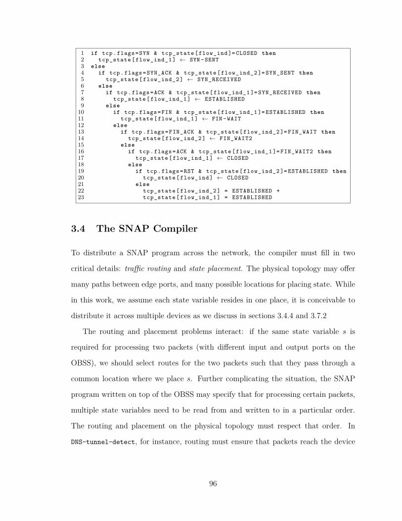
1 if tcp.flags=SYN & tcp_state [ flow_ind ]= CLOSED then2 tcp_state [ flow_ind_1 ] ← SYN -SENT3 else4 if tcp.flags= SYN_ACK & tcp_state [ flow_ind_2 ]= SYN_SENT then5 tcp_state [ flow_ind_2 ] ← SYN_RECEIVED6 else7 if tcp.flags=ACK & tcp_state [ flow_ind_1 ]= SYN_RECEIVED then8 tcp_state [ flow_ind_1 ] ← ESTABLISHED9 else

10 if tcp.flags=FIN & tcp_state [ flow_ind_1 ]= ESTABLISHED then11 tcp_state [ flow_ind_1 ] ← FIN -WAIT12 else13 if tcp.flags= FIN_ACK & tcp_state [ flow_ind_2 ]= FIN_WAIT then14 tcp_state [ flow_ind_2 ] ← FIN_WAIT215 else16 if tcp.flags=ACK & tcp_state [ flow_ind_1 ]= FIN_WAIT2 then17 tcp_state [ flow_ind_1 ] ← CLOSED18 else19 if tcp.flags=RST & tcp_state [ flow_ind_2 ]= ESTABLISHED then20 tcp_state [ flow_ind ] ← CLOSED21 else22 tcp_state [ flow_ind_2 ] = ESTABLISHED +23 tcp_state [ flow_ind_1 ] = ESTABLISHED

3.4 The SNAP Compiler

To distribute a SNAP program across the network, the compiler must fill in two

critical details: traffic routing and state placement. The physical topology may offer

many paths between edge ports, and many possible locations for placing state. While

in this work, we assume each state variable resides in one place, it is conceivable to

distribute it across multiple devices as we discuss in sections 3.4.4 and 3.7.2

The routing and placement problems interact: if the same state variable s is

required for processing two packets (with different input and output ports on the

OBSS), we should select routes for the two packets such that they pass through a

common location where we place s. Further complicating the situation, the SNAP

program written on top of the OBSS may specify that for processing certain packets,

multiple state variables need to be read from and written to in a particular order.

The routing and placement on the physical topology must respect that order. In

DNS-tunnel-detect, for instance, routing must ensure that packets reach the device

96

Figure 3.4: Overview of SNAP’s compiler phases.

where orphan is placed before the device storing susp-client. It is even possible for

different sets of packets to depend on the same state variables, but in different orders.

We have designed a compiler that translates SNAP programs into forwarding

rules and state placements for a given topology. As shown in Figure 3.4, the two

key phases are (i) translation to extended forwarding decision diagrams (xFDDs),

which is used as the intermediate representation of the program and to calculate

which flows need which state variables, and (ii) optimization via mixed integer linear

program (MILP), which is used to decide routing and state placement. In the rest

of this section, we present the compilation process in phases, first discussing the

analysis of state dependencies (section 3.4.1), followed by the translation to xFDDs

(section 3.4.2) and the packet-state mapping (section 3.4.3), then the optimization

problems (section 3.4.4), and finally generating configurations for network switches

(section 3.4.5).

3.4.1 State Dependency Analysis

Given a program, the compiler first performs state dependency analysis to determine

the ordering constraints on its state variables. A state variable t depends on a state

97

st-dep(p + q) = st-dep(p) ∪ st-dep(q)st-dep(p; q) = (r(p)×w(q)) ∪

st-dep(p) ∪ st-dep(q)st-dep(if a then p else q) = (r(a)× (w(p) ∪w(q)))

∪ st-dep(p) ∪ st-dep(q)st-dep(atomic(p)) = (r(a) ∪w(a))× (r(a) ∪w(a))

st-dep(p) = ∅ otherwise

r(p) : set of state variables read by pw(p) : set of state variables written by p

Figure 3.5: st-dep function for determining ordering constraints against state variables.

variable s if the program writes to t after reading from s. Any realization of the

program on a concrete network must ensure that for packets that required both

variables for their processing, the switch storing state variable t is not visited before

the one storing state variable s.

Figure 3.5 presents the st-dep function used by the compiler to extract state

dependencies from SNAP programs. Parallel composition, p + q, introduces no de-

pendencies: if p reads or writes state, then q can run independently of that. Sequential

composition p; q, on the other hand, introduces dependencies: whatever reads are in

p must happen before writes in q. In explicit conditionals “if a then p else q”, the

writes in p and q depend on the condition a. Finally, atomic sections atomic(p) say

that all state in p is inter-dependent. In DNS-tunnel-detect, for instance, blacklist

is dependent on susp-client, itself dependent on orphan. This information is encoded

as a dependency graph on state variables and is used to order the xFDD structure

(section 3.4.2), and in the MILP (section 3.4.4) to drive state placement.

3.4.2 Extended Forwarding Decision Diagrams

The input to the compiler is a SNAP program, which can be a composition of several

smaller programs. The output, on the other end, is the distribution of the original

policy across the network. Thus, in between, we need an intermediate representation

for SNAP programs that is both composable and easily partitioned. This intermediate98

representation can help the compiler compose small program pieces into a unified

representation, which can further be partitioned to get distributed across the network.

We use extended forwarding decision diagrams (xFDDs) as the intermediate rep-

resentation of SNAP programs in the compiler. xFDDs are inspired by forwarding

decision diagrams (FDDs) used for compiling programs composed of stateless predi-

cates and policies into switches with PISA-like architecture [92]. An FDD is a gen-

eralization of a binary decision diagram (BDD): each intermediate node is a test on

packet fields, and leaf nodes are sets of action sequences, rather than merely ‘true’

and ‘false’ as in a BDD [1]. Each intermediate node has two successors: true (solid

line), which determines the rest of the forwarding decision process for inputs passing

the test, and false (dashed line) for failed cases. An xFDD is an extension of an FDD

which supports stateful tests and actions as well.

Our decision to build the intermediate representation based on FDDs was driven

by the following:

• FDDs are tree-based data structures that provide a canonical representation of

the program by enforcing a certain ordering among the nodes in the tree. This

allows them, and their extension as xFDDs, to be both easily composed and

partitioned.

• FDDs lend themselves into efficient implementation on PISA-based architec-

tures. A PISA-based switch consist of a sequence of stages. Each stage has

a match-action table, which matches on user-defined bits in the packet and/or

user-defined metadata, and applies user-defined actions accordingly. Each path

from the root to leaf in an FDD (and by extension an xFDD) consists of se-

quence of boolean tests and a final set of actions, which fits nicely into the

capabilities of stages in PISA. Since we assume PISA-based architecture for the

switches in the network, FDDs are a suitable choice to extend and build our

stateful intermediate representation.99

d ::= t ? d1 : d2 | {as1, . . . , asn} xFDDst ::= f = v | f1 = f2 | s[e1] = e2 tests

as ::= a | a; a action sequencesa ::= id | drop | f ← v | s[e1]← e2 actions

| s[e1]++ | s[e1]--

Figure 3.6: xFDD syntax.

• They simplify analysis of SNAP programs for extracting packet-state mapping,

which we discuss in section 3.4.3.

Formally (see Figure 3.6), an xFDD is either a branch (t ? d1 : d2), where t is a test

and d1 and d2 are xFDDs, or a set of action sequences {as1, . . . , asn}. Each branch

can be thought of as a conditional: if the test t holds on a given packet pkt, then the

xFDD continues processing pkt using d1; if not, processes pkt using d2. There are

three kinds of tests:

• The field-value test f = v holds when pkt.f is equal to v.

• The field-field test f1 = f2 holds when the values in pkt.f1 and pkt.f2 are equal.

• The state test s[e1] = e2 holds when the state variable s at index e1 is equal to

e2.

The last two tests are our extensions to FDDs. The state tests support our stateful

primitives, and as we show later in this section, the field-field tests are required for

correct compilation. Each leaf in an xFDD is a set of action sequences, with each

action being either the identity, drop, field-update f ← v, or state update s[e1]← e2,

which is another extension to the original FDD.

A key property of xFDDs is that the order of their tests (@) must be defined in

advance. This ordering is necessary to ensure that each test is present at most once

on any path in the final tree when merging two xFDDs into one. That way, xFDD

composition can be done efficiently without creating redundant tests. In our xFDDs,

100

we ensure that all field-value tests precede all field-field tests, themselves preceding

all state tests.

Field-value tests themselves are ordered by fixing an arbitrary order on fields and

values. Field-field tests are ordered similarly. For state tests, we first define a total

order on state variables by looking at the dependency graph from section 3.4.1. We

break the dependency graph into strongly connected components (SCCs) and fix an

arbitrary order on state variables within each SCC. For every edge from one SCC to

another, i.e., where some state variable in the second SCC depends on some state

variable in the first, s1 precedes s2 in the order, where s2 is the minimal element in

the second SCC and s1 is the maximal element in the first SCC. The state tests are

then ordered based on the order of state variables.

We translate a program to an xFDD using the to-xfdd function (Figure 3.7),

which translates small parts of a program directly to xFDDs. Composite programs get

recursively translated and then composed using a corresponding composition operator

for xFDDs: we use ⊕ for composing the xFDDs of programs that are composed in

parallel, � for composing the xFDDs of programs that are sequentially composed,

and to negate the xFDD of predicates.

Figure 3.8 gives a high-level definition of the semantics of these operators. For

example, d1 ⊕ d2 tries to merge similar test nodes recursively by merging their true

branches together and false ones together. If the two tests are not the same and d1’s

test comes first in the total order, both of its subtrees are merged recursively with

d2. The other case is similar. d1 ⊕ d2 for leaf nodes is the union of their action sets.

The hardest case is surely for �, where we try to add in an action sequence as to

an xFDD (t ? d1 : d2). Suppose we want to compose f ← v1 with (f = v2 ? d1 : d2).

The result of this xFDD composition should behave as if we first do the update and

then the condition on f . If v1 = v2, the composition should continue only on d1, and

if not, only on d2. Now let’s look at a similar example including state, composing

101

to-xfdd(a) = {a}to-xfdd(f = v) = f = v ? {id} : {drop}

to-xfdd(¬x) = to-xfdd(x)to-xfdd(s[e1] = e2) = s[e1] = e2 ? {id} : {drop}to-xfdd(atomic(p)) = to-xfdd(p)

to-xfdd(p + q) = to-xfdd(p)⊕ to-xfdd(q)to-xfdd(p; q) = to-xfdd(p)� to-xfdd(q)

to-xfdd(if x then p else q) = (to-xfdd(x)� to-xfdd(p))⊕ (to-xfdd(x)� to-xfdd(q))

Figure 3.7: Translating SNAP programs into xFDDs using to-xfdd (See figure 3.8 for thedefinition of the xFDD composition operators).

s[srcip] ← e1 with (s[dstip] = e2 ? d1 : d2). If srcip and dstip are equal (rare but

not impossible) and e1 and e2 always evaluate to the same value, then the whole

composition reduces to just d1. The field-field tests are introduced to let us answer

these equality questions, and that is why they always precede state tests in the tree.

The trickiness in the algorithm comes from generating proper field-field tests, by

keeping track of the information in the xFDD, to properly answer the equality tests

of interest. The full algorithm is discussed at the end of this section.

Note that the actual definition of the composition operators is a bit more involved

than the one in Figure 3.8 as we have to make sure, while composing xFDDs, that

the resulting xFDD is well-formed. An xFDD is defined to be well-formed if its tests

conform to the pre-defined total order (@) and do not contradict the previous tests

in the xFDD. Figure 3.9 contains a more detailed definition of ⊕ as an example.

To detect possible contradictions, we accumulate both the equalities and inequalities

implied by previous tests in an argument called context and pass it through recursive

calls to ⊕. Before applying ⊕ to the input xFDDs, we first run each of the FDDs

through a function called refine, which removes both redundant and contradicting

tests from top of the input FDD based on the input context until it reaches a non-

redundant and non-contradicting test. After both input FDDs are “refined”, we

continue with the merge as before.

102

Composition Operator ⊕ (used for p + q)

{as11, · · · , as1n} ⊕ {as21, · · · , as2m} = {as11, · · · , as1n} ∪ {as21, · · · , as2m}(t ? d1 : d2)⊕ {as1, · · · , asn} = (t ? d1 ⊕ {as1, · · · , asn} : d2 ⊕ {as1, · · · , asn})

(t1 ? d11 : d12)⊕ (t2 ? d21 : d22) =

(t1 ? d11 ⊕ d21 : d12 ⊕ d22) t1 = t2

(t1 ? d11 ⊕ (t2 ? d21 : d22) : d12 ⊕ (t2 ? d21 : d22) t1 @ t2

(t2 ? d21 ⊕ (t1 ? d11 : d12) : d22 ⊕ (t1 ? d11 : d12) t2 @ t1

Composition Operator (used for ¬p)

{id} = {drop}{drop} = {id}

(t?d1 : d2) = (t? d1 : d2)

Composition Operator � (used for p; q)

as� {as1, · · · , asn} = {as� as1, · · · , as� asn}as� (t ? d1 : d2) = (see explanations in section 3.4.2){as1, · · · , asn} � d = (as1 � d)⊕ · · · ⊕ (asn � d)(t ? d1 : d2)� d = (d1 � d)|t ⊕ (d2 � d)|∼t

Operator |t (used in �)

{as1, · · · , asn}|t = (t ? {as1, · · · , asn} : {drop})

(t1 ? d1 : d2)|t2 =

(t1 ? d1 : {drop}) t1 = t2

(t2 ? (t1 ? d1 : d2) : {drop}) t2 @ t1

(t1 ? d1|t2 : d2|t2 ) t1 @ t2

Figure 3.8: xFDD composition operators.

Finally, recall from section 3.2 that inconsistent use of state variables is prohibited

by the language semantics when composing programs. We enforce the semantics by

looking for these violations while merging the xFDDs of composed programs and

raising a compile error if the final xFDD contains a leaf with parallel updates to the

same state variable.

A Deeper Look into the Sequential Composition of xFDDs

We conclude this section with a high-level pseudocode for the base case of sequential

composition, namely when composing one action sequence with another FDD (Algo-

rithms 1). Apart from the composition operands, function seq (Algorithm 1) has a

third argument, T , which is the context we introduced earlier in this section and used

for refining xFDDs during composition (Figure 3.9).

103

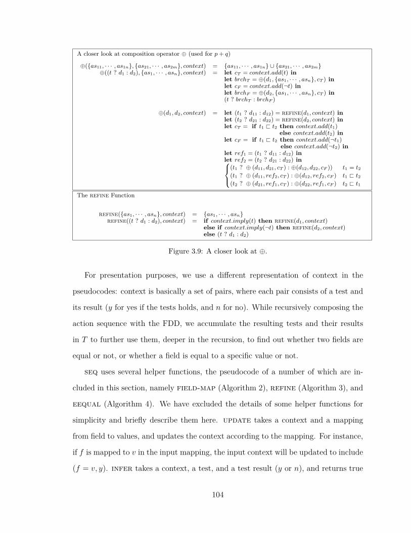
A closer look at composition operator ⊕ (used for p + q)

⊕({as11, · · · , as1n}, {as21, · · · , as2m}, context) = {as11, · · · , as1n} ∪ {as21, · · · , as2m}⊕((t ? d1 : d2), {as1, · · · , asn}, context) = let cT = context.add(t) in

let brchT = ⊕(d1, {as1, · · · , asn}, cT ) inlet cF = context.add(¬t) inlet brchF = ⊕(d2, {as1, · · · , asn}, cT ) in(t ? brchT : brchF )

⊕(d1, d2, context) = let (t1 ? d11 : d12) = refine(d1, context) inlet (t2 ? d21 : d22) = refine(d2, context) inlet cT = if t1 @ t2 then context.add(t1)

else context.add(t2) inlet cF = if t1 @ t2 then context.add(¬t1)

else context.add(¬t2) inlet ref1 = (t1 ? d11 : d12) inlet ref2 = (t2 ? d21 : d22) in(t1 ? ⊕ (d11, d21, cT ) : ⊕(d12, d22, cF )) t1 = t2

(t1 ? ⊕ (d11, ref2, cT ) : ⊕(d12, ref2, cF ) t1 @ t2

(t2 ? ⊕ (d21, ref1, cT ) : ⊕(d22, ref1, cF ) t2 @ t1

The refine Function

refine({as1, · · · , asn}, context) = {as1, · · · , asn}refine((t ? d1 : d2), context) = if context.imply(t) then refine(d1, context)

else if context.imply(¬t) then refine(d2, context)else (t ? d1 : d2)

Figure 3.9: A closer look at ⊕.

For presentation purposes, we use a different representation of context in the

pseudocodes: context is basically a set of pairs, where each pair consists of a test and

its result (y for yes if the tests holds, and n for no). While recursively composing the

action sequence with the FDD, we accumulate the resulting tests and their results

in T to further use them, deeper in the recursion, to find out whether two fields are

equal or not, or whether a field is equal to a specific value or not.

seq uses several helper functions, the pseudocode of a number of which are in-

cluded in this section, namely field-map (Algorithm 2), refine (Algorithm 3), and

eequal (Algorithm 4). We have excluded the details of some helper functions for

simplicity and briefly describe them here. update takes a context and a mapping

from field to values, and updates the context according to the mapping. For instance,

if f is mapped to v in the input mapping, the input context will be updated to include

(f = v, y). infer takes a context, a test, and a test result (y or n), and returns true

104

if the specified test result can be inferred from the context for the given test. value

takes in a context and a field f . If it can be inferred from the context that f = v,

value returns v, and returns f otherwise. Finally, reverse reverses the input list.

Algorithm 11: a is a sequence of actions2: d is an FDD in the form of (t ? d1 : d2)3: T is a set of (test, res ∈ {y, n})4:5: function seq(a, d, T )6: (t ? d1 : d2)← d7: if t == {f = v} then8: fmap← field-map(a)9: if f ∈ fmap then10: if fmap[f ] == v then11: return seq(a, d1, T )12: else13: return seq(a, d2, T )14: end if15: else16: d′

1 ← seq(a, d1, T ∪ {(f = v, y)})17: d′

2 ← seq(a, d2, T ∪ {(f = v, n)})18: return (f = v ? d′

1 : d′2)

19: end if20: else if t == {f1 = f2} then21: fmap← field-map(a)22: if f1 ∈ fmap ∧ f2 ∈ fmap then23: v1 ← fmap[f1]24: v2 ← fmap[f2]25: if v1 = v2 then26: return seq(a, d1, T )27: else28: return seq(a, d2, T )29: end if30: else31: f ′

1 ← fmap[f1] if f1 ∈ fmap else f132: f ′

2 ← fmap[f2] if f2 ∈ fmap else f2

33: d′1 ← seq(a, d1, T ∪ {(f ′

1 = f ′2, y)})

34: d′2 ← seq(a, d2, T ∪ {(f ′

1 = f ′2, n)})

35: return (f ′1 = f ′

2 ? d′1 : d′

2)36: end if37: else if t == {s[e1] = e2} then38: a′ ← refine(a, s)39: a′ ← reverse(a′)40: for s[e3] := e4 ∈ a′ do41: (eq, test)← eequal(e1, e3)42: if eq == y then43: (eq2, test2)← eequal(e2, e4)44: if eq2 == y then45: return seq(a, d1, T )46: else if eq2 == n then47: return seq(a, d2, T )48: else if eq2 == both then49: d′ ← (test2 ? d : d)50: return seq(a, d′, T )51: end if52: else if eq == n then53: continue54: else if eq == both then55: d′ ← (test ? d : d)56: return seq(a, d′, T )57: end if58: end for59: d′

1 ← seq(a, d1, T ∪ {(s[e1] = e2, y)})60: d′

2 ← seq(a, d2, T ∪ {(s[e1] = e2, n)})61: return (f = v ? d′

1 : d′2)

62: end if63: end function

Algorithm 21: a is a sequence of actions2: function field-map(a)3: fmap← empty dictionary . A dictionary from packet fields to values4: for act ∈ a do5: if act == (f ← v) then6: fmap[f ]← v7: else if act == drop then8: break9: end if10: end for11: return fmap12: end function

105

Algorithm 31: a is a sequence of actions2: s is a state variable3:4: function refine(a, s)5: fmap← empty dictionary . A dictionary from packet fields to values6: for act ∈ a do7: if act == 1 then8: continue9: else if act == 0 then10: break11: else if act == (f ← v) then12: fmap[f ]← v13: else if act == (x[e1] := e2) then14: replace each occurrence of a packet field15: in e1 and e2 with their value in16: the dictionary if present17: end if18: end for19: a′ ← empty sequence20: for act ∈ a do21: if act == (x[e1] := e2) ∧ x == s then22: a′.add(act)23: end if24: end for25: return a′

26: end function

Algorithm 41: e1 and e2 are expressions2: T is a set of (test, res ∈ {y, n})3:4: function eequal(e1, e2, T )5: if e1.length 6= e2.length then6: return (false,−)7: end if8: res← (true,−)9: for 0 ≤ i < e1.length do10: if e1[i] == e2[i] ∨ (e1[i] = e2[i] inferred from T ) then11: continue12: else if (e1[i] = e2[i], n) inferred from T then13: return (false,−)14: else15: if there is a e1[i] = v1 in T then16: return (both, (e2[i] = v1))17: else if there is a e2[i] = v2 in T then18: return (both, (e1[i] = v2))19: else20: return (both, (e1[i] = e2[i]))21: end if22: end if23: end for24: return res25: end function

106

3.4.3 Packet-State Mapping

For a given program p, the corresponding xFDD d offers an explicit and complete

specification of the way p handles packets. We analyze d, using an algorithm called

packet-state mapping, to determine which flows use which states. This information is

further used in the optimization problem (section 3.4.4) to decide the correct routing

for each flow. Our default definition of a flow is the set of packets that travel between

any given pair of ingress/egress ports in the OBS, though we can use other notions

of flow (see section 3.4.4).

Traversing from d’s root down to the actions at d’s leaves, we can gather informa-

tion about which set of state variables may be read or written when processing packets

of each flow. For instance, suppose we traverse the xFDD for DNS-tunnel-detect ;

assign-egress (depicted in figure 3.2) from root to leaf 5. Based on the actions in

leaf 5, we can deduce that processing some packets from flows to port 1 may involve

updates to orphan and susp-client state variables. Moreover, based on the test in

node 3 which is on the path from root to leaf 5, we can deduce that processing those

packets involves reading from orphan as well.

Furthermore, the operators can give hints to the compiler by specifying their

network assumptions in a separate policy:

1 assumption = (srcip = 10.0.1.0/24 & inport = 1)2 + (srcip = 10.0.2.0/24 & inport = 2)3 + ...4 + (srcip = 10.0.6.0/24 & inport = 6)

We require the assumption policy to be a predicate over packet header fields,

only passing the packets that match the operator’s assumptions. assumption is then

sequentially composed with the rest of the program, enforcing the assumption by

dropping packets that do not match the assumption.

Such assumptions benefit the packet-state mapping. Consider our example xFDD

in Figure 3.2. Following the xFDD’s tree structure, we can infer that all the packets107

going to port 6 need all the three state variables in DNS-tunnel-detect. We can

also infer that all the packets coming from the 10.0.6.0/24 subnet need orphan and

susp-client. However, there is nothing in the program to tell the compiler that these

packets can only enter the network from port 6. Thus, the above assumption policy

can help the compiler to identify this relation and place state more efficiently.

3.4.4 State Placement and Routing

At this stage, the compiler has enough information to fill in the details abstracted

away from the programmer: where and how each state variable should be placed, and

how the traffic should be routed in the network.

There are two general approaches for deciding state placement and routing. One

is to keep only one copy of each state variable at one location and route the traffic

through the state variables needed for its processing. The other is to keep multiple

copies of the same state variable on different switches and partition and route the

traffic through them. The second approach requires mechanisms to keep different

copies of the same state variable consistent. However, it is not possible to provide

strong consistency guarantees when distributed updates are made on a packet-by-

packet basis at line rate. Therefore, we chose the first approach, which locates each

state variable at one physical switch. Note that in this approach, it is still possible

to distribute a state variable by partitioning, as opposed to copying, it into multiple

independent state variables. We will discuss such extensions at the end of this section.

To decide state placement and routing, we generate an optimization problem, a

mixed-integer linear program (MILP) that is an extension of the multi-commodity

flow linear program. The MILP has three key inputs: the concrete network topology,

the state dependency graph G, and the packet-state mapping, and two key outputs:

routing and state placement (Table 3.2). Since route selection depends on state

placement and each state variable is constrained to one physical location, we need

108

Variable Descriptionu, v edge nodes (ports in OBS)n physical switches in the network

i, j all nodes in the networkduv traffic demand between u and vcij link capacity between i and jdep state dependenciestied co-location dependenciesSuv state variables needed for flow uv

Ruvij fraction of duv on link (i, j)Psn 1 if state s is placed on n, 0 otherwise

Psuvij duv fraction on link (i, j) that has passed s

Table 3.2: Inputs and outputs of the optimization problem.

to make sure the MILP picks correct paths without degrading network performance.

Thus, the MILP minimizes the sum of link utilization in the network as a measure

of congestion. However, other objectives or constraints are conceivable to customize

the MILP to other kinds of performance requirements.

Inputs. The topology is defined in terms of the following inputs to the MILP:

• the nodes, some distinguished as edges (ports in OBSS),

• expected traffic duv for every pair of edge nodes u and v, and

• link capacities cij for every pair of nodes i and j.

State dependencies in G are translated into input sets dep and tied. tied contains

pairs of state variables which are in the same strongly connected component (SCC)

in G, and must be co-located. dep identifies state variables with dependencies that

do not need to be co-located; in particular, (s, t) ∈ dep when s precedes t in variable

ordering, and they are not in the same SCC in G. The packet-state mapping is used as

the input variables Suv, identifying the set of state variables needed on flows between

nodes u and v.

Outputs and Constraints. The routing outputs are variables Ruvij, indicating

what fraction of the flow from edge node u to v should traverse the link between nodes

109

i and j. The constraints on Ruvij (left side of Table 3.3) follow the multi-commodity

flow problem closely, with standard link capacity and flow conservation constraints,

and edge nodes distinguished as sources and sinks of traffic.

State placement is determined by the variables Psn, which indicate whether the

state variable s should be placed on the physical switch n. Our constraints here are

more unique to our setting:

• First, every state variable s can be placed on exactly one switch to avoid syn-

chronization overheads for providing consistency across multiple copies on dif-

ferent switches. That said, we discuss later in this section how to potentially

relax this constraint by sharding a state variable into partitions that can be

placed independently and without synchronization overhead.

• Second, we must ensure that flows that need a given state variable s traverse

that switch.

• Third, we must ensure that each flow traverses states in the order specified

by the dep relation; this is what the variables Psuvij are for. We require that

Psuvij = Ruvij when the traffic from u to v that goes over the link (i, j) has

already passed the switch with the state variable s, and zero otherwise. If dep

requires that s should come before some other state variable t—and if the (u, v)

flow needs both s and t—we can use Psuvij to make sure that the (u, v) flow

traverses the switch with t only after it has traversed the switch with s (the last

state constraint in Table 3.3).

• Finally, we must make sure that state variables (s, t) ∈ tied are located on

the same switch. Note that only state variables that are inter-dependent are

required to be located on the same switch. Two variables s and t are inter-

dependent if a read from s is required before a write to t and vice versa. Plac-

ing them on different switches will result in a forwarding loop between the two110

Routing Constraints State Constraints∑n Psn = 1∑

j Ruvuj = 1 ∀u, v. ∀s ∈ Suv.∑

i Ruvin ≥ Psn∑i Ruviv = 1 ∀(s, t) ∈ tied. Psn = Ptn∑u,v Ruvijduv ≤ cij Psuvij ≤ Ruvij∑i Ruvin =

∑j Ruvnj Psn + ΣiPsuvin = ΣjPsuvnj∑

i Ruvin ≤ 1 ∀s ∈ Suv. Psv +∑

i Psuviv = 1Psn + ΣiPsuvin ≥ Ptn

Table 3.3: Constraints of the optimization problem.

switches which is not desirable in most networks. Therefore, in order to syn-

chronize reads and writes to inter-dependent variables correctly, they are always

placed on the same switch.

Although the current prototype chooses the same path for the traffic between the

same ports, the MILP can be configured to decide paths for more fine-grained notions

of flows. Suppose packet-state mapping finds that only packets with srcip = x need

state variable s. We refine the MILP input to have two edge nodes per port, one for

traffic with srcip = x and one for the rest, so the MILP can choose different paths

for them.

Note that in our prototype, the MILP assigns each state variable to one physical

switch to avoid the overhead of synchronizing multiple instances of the same variable.

Still, distributing a state variable remains a valid option. Consider s[inport] for

instance. The compiler can partition s into s1 to sk, where si stores s for port i. The

MILP can be used as before to decide placement and routing, this time with the option

of placing si variables at different places without worrying about synchronization as si

variables store disjoint parts of s. The same idea can be used for distributing t[srcip],

where t1 to tk are t’s partitions for disjoint subset of IP addresses ip1 to ipk. In this

case, each port u in the OBSS should be replaced with u1 to uk, with ui handling u’s

traffic with source IP ipi. We leave an implementation of this optimization to future

work.

111

Finally, the MILP makes a joint decision for state placement and routing. There-

fore, path selection is tied to state placement. To have more freedom in picking

forwarding paths, one option is to first use common traffic engineering techniques to

decide routing, and then optimize the placement of state variables with respect to

the selected paths. However, this approach may require replicating state variables

and maintaining consistency across multiple copies, which as mentioned earlier, is

not possible at line rate for distributed packet-by-packet updates to state variables.

3.4.5 Generating Switch Configurations

Switch configurations are generated in two phases, combining information from the

xFDD and MILP. We assume each packet is augmented with a SNAP-header upon

entering the network, which contains fields for its original OBSS input port and future

output port, and the id of the last processed xFDD node, the purpose of which will

be explained shortly. This header is stripped off by the egress switch when the packet

exits the network. We use DNS-tunnel-detect;assign-egress from section 3.1 as a

running example, with its xFDD in Figure 3.2. For the sake of the example, we

assume that all the state variables are stored on C6 instead of D4.

In the first phase, we break the xFDD down into ‘per-switch’ xFDDs, since not ev-

ery switch needs the entire xFDD to process packets. Splitting the xFDD is straight-

forward given placement information: stateless tests and actions can happen any-

where, but reads and writes of state variables must happen on switches storing them.

For example, edge switches (I1 and I2, and D1 to D4) only need to process packets

up to the state tests, e.g., tests 3 and 8, and write the test number in the packet’s

SNAP-header showing how far into the xFDD they progressed. Then, they send the

packets to C6, which has the corresponding state variables, orphan and susp-client.

C6, on the other hand, does not need the top part of the xFDD. It just needs the

subtrees containing its state variables to continue processing the packets sent from

112

the edges. The per-switch xFDDs are then translated to switch-level configurations,

by a straightforward traversal of the xFDD (see section 3.5).

In the second phase, we generate a set of match-action rules that take packets

through the paths decided by the MILP. These paths comply with the state ordering

used in the xFDD, thus they get packets to switches with the right states in the right

order. Note that packets contain the path identifier (the OBSS inport and outport,

(u, v) pair in this case) and the “routing” match-action rules are generated in terms of

this identifier to forward them on the correct path. Additionally, note that it may not

always be possible to decide the egress port v for a packet upon entry if its outport

depends on state. We observe that in that case, all the paths for possible outports

of the packet pass the state variables it needs. We load-balance over these paths in

proportion to their capacity and show that traffic on these paths remains in their

capacity limit.

More specifically, suppose a packet arrives at port 1 in our example topology and

the user policy specifies that its outport should be assigned to either 5 or 6 based on

state variable s, located at C6. Assume the MILP assigns the path p1 to (1, 5) traffic

and the path p2 to (1, 6). The ingress switch (I1) can not determine whether the

packet belongs to (1, 5) or (1, 6) to forward it on p1 or p2 respectively. But, it does

not actually matter. Both paths go through C6 because s is required for processing

both kinds of traffic. In order to ensure better usage of resources, we can choose

which of p1 and p2 to send the packet over in proportion to each path’s capacity.

But whichever path we take, the packet will make its way to C6 and its processing

continues from there.

More formally, the MILP outputs the optimized path for the traffic between each

ingress port u and egress port v. However, the policy may not be able to determine

v at the ingress switch. Suppose that v1, · · · , vk are the possible outport for packets

that enter from u. From packet-state mapping (section 3.4.3), we know that the

113

packets from u to each vi need a sequence (as they are now ordered) of state variables

< si1, · · · , sip >. Therefore, the designated path for this traffic goes through the

sequence of nodes < u, ni1, · · · , nip, vi > where nij is the switch holding sij. Now

suppose that the policy starts processing a packet from inport u and gets stuck on a

statement containing s. If s only appears in vi’s state sequence, the policy’s getting

stuck on s implies that the packet belongs to the traffic from u to vi, so we can safely

forward the packet on its designated path.

However, it may be the case that s appears in the state sequences of multiple

outports. Let’s call the set of outports vi whose traffic need s, Vs, and assume that s

appears in the state sequence of vi at index li. Thus, we have multiple paths to the

switch holding s, where the path assigned to (u, vi)’s traffic is < u, ni1, · · · , nili > and

is capable of carrying at least duvivolume of traffic. The observation here is that at

most ∑vi∈Vs

duviworth of traffic entering from u needs state s, and the total capacity

of the designated paths from u to nili , where s is held, is also equal to ∑vi∈Vs

duvi.

Therefore, we just send the traffic that needs s over one of these paths in proportion

to their capacity. The packet will make its way to the switch holding s, and its

processing will continue from there.

As an example of how packets are handled by the switches based on the generated

configurations, consider a DNS response with source IP 10.0.1.1 and destination IP

10.0.6.6, entering the network from port 1. The rules on I1 process the packet up to

test 8 in the xFDD, tag the packet with the path identifier (1, 6) and number 8. The

packet is then sent to C6. There, C6 will process the packet from test 8, update state

variables accordingly, and send the packet to D4 to exit the network from port 6.

3.5 Implementation

The compiler is mostly implemented in Python, except for the state placement and

routing phase (section 3.4.4) which uses the Gurobi Optimizer [36] to solve the MILP.

114

The compiler’s output for each switch is a set of switch-level instructions in a low-

level language called NetASM [88], which comes with a software switch capable of

executing those instructions. NetASM is an assembly language for programmable

data planes designed to serve as the “narrow waist” between high-level languages

such as SNAP, and NetCore [62], and programmable switching architectures such as

PISA (and RMT [13]) as well as FPGAs, network processors and Open vSwitch.

As described in section 3.4.5, each switch processes the packet by its customized

per-switch xFDD, and then forwards it based on the fields of the SNAP-header us-

ing a match-action table. To translate the switch’s xFDD to NetASM instructions,

we traverse the xFDD and generate a branch instruction for each test node, which

jumps to the instruction of either the true or false branch based on the test’s result.

Moreover, we generate instructions to create two tables for each state variable, one

for the indices and one for the values. In the case of a state test in the xFDD, we

first retrieve the value corresponding to the index that matches the packet, and then

perform the branch. For xFDD leaf nodes, we generate store instructions that modify

the packet fields and state tables accordingly. Finally, we use NetASM support for

atomic execution of multiple instructions to guarantee that operations on state tables

happen atomically.

NetASM’s software switch support for atomic operations on match-action tables

was useful for testing our compiler. As a result, in our current prototype, it is used

as the target for which the compiler generates configurations. However, any pro-

grammable switch hardware that supports match-action tables, branch instructions,

and stateful operations can be a SNAP target. More specifically, in PISA-based

switches, the prioritized rules in match-action tables, for instance, are effectively

branch instructions. Thus, one can use multiple match-action tables to implement

xFDD in PISA-based switches that support prioritized rules in their match-action

tables by generating a separate rule for each path in the xFDD.

115

Moreover, emerging PISA-based switches allow for stateful operations in their

packet processing stages [39, 69, 103, 106], which can be used to implement reads

and writes to SNAP’s state variables. A state variable (array) in SNAP is a key-

value mapping, or a dictionary, on header fields, persistent across multiple packets.

When the key (index) range is small, it is feasible to pre-allocate all the memory the

dictionary needs and implement it using an array. A large but sparse dictionary can

be implemented using a reactively-populated table, similar to a MAC learner table.

It contains a single default entry in the beginning, and as packets fly by and change

the state variable, it reactively adds/updates the corresponding entries.

There are two main options for implementing a dictionary using either approach

in high-speed switch hardware:

• Arrays of registers. Emerging programmable switches support reading from

and writing to arrays of registers at high-speed [69, 103]. They can be used to

implement small dictionaries, as well as Bloom Filters and hash tables as sparse

dictionaries. In the latter case, it is possible for two different keys to hash to the

same dictionary entry. However, there are applications such as load balancing

and flow-size-based sampling that can tolerate such collisions [65].

• Content Addressable Memories (CAMs). CAMs are typically present in

today’s hardware switches and can be modified by a software agent running

on the switch. Since CAM updates triggered by a packet are not immediately

available to the following packets, it may be used for applications that tolerate

small periods of state inconsistency, such as a MAC learner, DNS tunnel detec-

tion, and others from Table 3.1. We used this approach in an initial version of

our prototype, in which the compiler generated P4 [12] programs to configure

PISA-based switches.

116

At the time of writing this dissertation, we are not aware of any hardware switch

that can implement an arbitrary number of SNAP’s stateful operations both at line

rate and with strong consistency. This is another reason why, in our current prototype,

we chose NetASM’s low-level primitives over P4 as the compiler backend. This way,

we can specify data-plane primitives that are required for an efficient and consistent

implementation of SNAP’s operations. If one is willing to relax one of the above

constraints for a specific application, i.e., operating at line rate or strong consistency,

it would be possible to implement SNAP on today’s hardware switches. If strong

consistency is relaxed, CAMs/TCAMs can be programmed using languages such as

P4 [12] (similar to our initial prototype) to implement SNAP’s stateful operations

as described above. If line-rate processing is relaxed, one can use software switches,

or programmable hardware switching devices such NPUs, FPGAs, or those in the

OpenNFP project that allow insertion of Micro-C code extensions to P4 programs at

the expense of processing speed [74].

3.6 Evaluation

This section evaluates SNAP in terms of language expressiveness and compiler per-

formance.

3.6.1 Language Expressiveness

We have implemented several stateful network functions that are either present or

needed in modern networks SNAP (Table 3.1). Examples were taken from the

Chimera [11], FAST [65], and Bohatei [22] systems, and can be found in section 3.3.

Most examples use protocol-related fields in fixed packet-offset locations, which are

parsable by programmable parsers in PISA-based switches. Some fields require ses-

sion reassembly. However, this is orthogonal to the language expressiveness; as long as

these fields are available to the switch, they can be used in SNAP programs. To make

117

them available, one could extract these fields by placing a “preprocessor” before the

switch pipeline, similar to middleboxes. For instance, Snort [93] uses preprocessors

to extract fields for use in the detection engine.

3.6.2 Compiler Performance

The compiler goes through several phases upon the system’s cold start. However, in

responding to most events, it requires to re-execute only some of them. Table 3.4

summarizes these phases and their sensitivity to network and policy changes. There

are three different scenarios in which the compiler needs to execute all of some of its

phases:

• Cold Start. When the very first program is compiled, the compiler goes

through all phases, including MILP model creation, which happens only once

in the lifetime of the network. Once created, the model supports incremental

additions and modifications of variables and constraints in a few milliseconds.

• Policy Changes. Compiling a new program requires executing the three pro-

gram analysis phases and rule generation as well as both state placement and

routing, which are decided using the MILP in section 3.4.4, denoted by “ST”.

Policy changes become considerably less frequent (section 3.1.2) since most dy-

namic changes are captured by the state variables that reside on the data plane.

The policy, and consequently switch configurations, do not change upon state

changes. Thus, we expect policy changes to happen infrequently, and be planned

in advance. The Snort rule set, for instance, gets updated every few days [94].

• Topology/TM Changes. Once the policy is compiled, we fix the decided state

placement, and only re-optimize routing in response to network events such as

failures. For that, we do not need to run our original MILP, denoted as “ST”

(standard). We formulated a variant of ST MILP, denoted as “TE” (traffic

118

ID Phase Topology/TM Change Policy Change Cold StartP1 State dependency - X XP2 xFDD generation - X XP3 Packet-state map - X XP4 MILP creation - - X

P5 MILPsolving

State placementand routing (ST) - X X

Routing (TE) X - -P6 Rule generation X X X

Table 3.4: Compiler phases. For each scenario, phases that get executed are checkmarked.

engineering), that receives state placement as input, and decides forwarding

paths while satisfying state requirement constraints. We expect TE to run every

few minutes since in a typical network, the traffic matrix is fairly stable and

traffic engineering happens on the timescale of minutes [40, 71,97,102].

Experiments

We evaluated performance based on applications listed in Table 3.1. Traffic matrices

are synthesized using a gravity model [83]. We used an Intel Xeon E3, 3.4 GHz, 32GB

server, and PyPy [78] to run the compiler.

Benchmark Topologies. We used a set of three campus networks and four

inferred ISP topologies from RocketFuel [96] (Table 3.5).1 For ISP networks, we

considered 70% of the switches with the lowest degrees as edge switches to form

OBSS external ports. The “# Demands” column shows the number of distinct OBSS

ingress/egress pairs. We assume directed links. Table 3.6 shows compilation time for

the DNS tunneling example (section 3.1) on each network, broken down by compiler

phase. Figure 3.10 compares the compiler runtime for different scenarios, combining

the runtimes of phases relevant for each.

Scaling with topology size. We synthesize networks with 10–180 switches

using IGen [80]. In each network, 70% of the switches with the lowest degrees are

chosen as edges and the DNS tunnel policy is compiled with that network as a target.1 The publicly available Mininet instance of Stanford campus topology has 10 extra dummy switches to implementmultiple links between two routers.

119

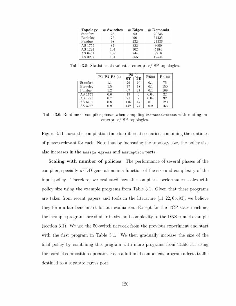
Topology # Switches # Edges # DemandsStanford 26 92 20736Berkeley 25 96 34225Purdue 98 232 24336AS 1755 87 322 3600AS 1221 104 302 5184AS 6461 138 744 9216AS 3257 161 656 12544

Table 3.5: Statistics of evaluated enterprise/ISP topologies.

P1-P2-P3 (s) P5 (s) P6(s) P4 (s)ST TEStanford 1.1 29 10 0.1 75Berkeley 1.5 47 18 0.1 150Purdue 1.2 67 27 0.1 169AS 1755 0.6 19 6 0.04 22AS 1221 0.7 21 7 0.04 32AS 6461 0.8 116 47 0.1 120AS 3257 0.9 142 74 0.2 163

Table 3.6: Runtime of compiler phases when compiling DNS-tunnel-detect with routing onenterprise/ISP topologies.

Figure 3.11 shows the compilation time for different scenarios, combining the runtimes

of phases relevant for each. Note that by increasing the topology size, the policy size

also increases in the assign-egress and assumption parts.

Scaling with number of policies. The performance of several phases of the

compiler, specially xFDD generation, is a function of the size and complexity of the

input policy. Therefore, we evaluated how the compiler’s performance scales with

policy size using the example programs from Table 3.1. Given that these programs

are taken from recent papers and tools in the literature [11, 22, 65, 93], we believe

they form a fair benchmark for our evaluation. Except for the TCP state machine,

the example programs are similar in size and complexity to the DNS tunnel example

(section 3.1). We use the 50-switch network from the previous experiment and start

with the first program in Table 3.1. We then gradually increase the size of the

final policy by combining this program with more programs from Table 3.1 using

the parallel composition operator. Each additional component program affects traffic

destined to a separate egress port.

120

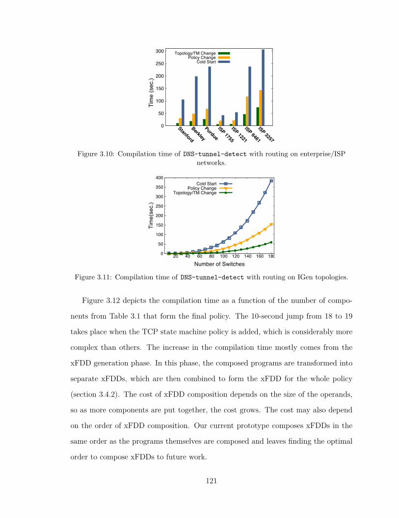
0

50

100

150

200

250

300

Stanford

Berkley

Purdue

ISP 1755

ISP 1221

ISP 6461

ISP 3257

Tim

e (s

ec.)

Topology/TM ChangePolicy Change

Cold Start

Figure 3.10: Compilation time of DNS-tunnel-detect with routing on enterprise/ISPnetworks.

0

50

100

150

200

250

300

350

400

20 40 60 80 100 120 140 160 180

Tim

e(se

c.)

Number of Switches

Cold StartPolicy Change

Topology/TM Change

Figure 3.11: Compilation time of DNS-tunnel-detect with routing on IGen topologies.

Figure 3.12 depicts the compilation time as a function of the number of compo-

nents from Table 3.1 that form the final policy. The 10-second jump from 18 to 19

takes place when the TCP state machine policy is added, which is considerably more

complex than others. The increase in the compilation time mostly comes from the

xFDD generation phase. In this phase, the composed programs are transformed into

separate xFDDs, which are then combined to form the xFDD for the whole policy

(section 3.4.2). The cost of xFDD composition depends on the size of the operands,

so as more components are put together, the cost grows. The cost may also depend

on the order of xFDD composition. Our current prototype composes xFDDs in the

same order as the programs themselves are composed and leaves finding the optimal

order to compose xFDDs to future work.

121

0

10

20

30

40

50

4 6 8 10 12 14 16 18 20

Tim

e(se

c.)

Number of Composed Policies

Cold StartPolicy Change

Topology-TM Change

Figure 3.12: Compilation time for policies from Table 3.1 incrementally composed on a50-switch network.

The last data point in Figure 3.12 shows the compilation time of a policy composed

of all the 20 examples in Table 3.1, with a total of 35 state variables. These policies

are composed using parallel composition, which does not introduce read/write depen-

dencies between state variables. Thus, the dependency graph for the final policy is a

collection of the dependency graphs of the composed policies. Each of the composed

policies affects the traffic to a separate egress port, which is detected by the compiler

in the packet-state mapping phase. Thus, when compiled to the 50-switch network,

state variables for each policy are placed on the switch closest to the egress port

whose traffic the policy affects. If a policy were to affect a larger portion of traffic,

e.g., the traffic of a set of ingress/egress ports, SNAP would place state variables in

an optimal location where the aggregated traffic of interest is passing through.

Analysis of Experimental Results

There are three key takeaways from the results of our experiments:

• Creating the MILP takes longer than solving it, in most cases, and much longer

than other phases. Fortunately, this is a one-time cost. After creating the

MILP instance, incrementally adding or removing variables and constraints (as

the topology and/or state requirements change) takes just a few milliseconds.

122

• Solving the ST MILP unsurprisingly takes longer as compared to the rest of the

phases when topology grows. It takes ∼ 2.5 minutes for the biggest synthesized

topology and ∼ 2.3 minutes for the biggest RocketFuel topology. The curve is

close to exponential as the problem is inherently computationally hard. How-

ever, this phase takes place only in cold start or upon a policy change, which

are infrequent and planned in advance.

• Re-optimizing routing with fixed state placement is much faster. In response to

network events (e.g., link failures), TE MILP can recompute paths in around a

minute across all our experiments, which is the timescale we initially expected for

this phase as it runs in the topology/TM change scenarios. Moreover, it can be

used even on policy changes, if the user settles for a sub-optimal state placement

using heuristics rather than ST MILP. We leave a detailed exploration of such

heuristics to future work.

Given the kinds of events that require complete (policy change) or partial (net-

work events) recompilation, we believe that our compilation techniques meet the

requirements of enterprise networks and medium-size ISPs. Moreover, if needed, our

compilation procedure could be combined with traffic-engineering techniques once the

state placement is decided, to avoid re-solving the original or even TE MILP on small

timescales.

3.7 Discussion

This section discusses how SNAP relates to middleboxes and possible extensions to

our techniques to enable a broader range of applications.

123

3.7.1 SNAP and Middleboxes

The increasing need for stateful packet processing inside the network together with the

fact that early switches were only capable of stateless packet processing, has caused

network operators to mostly rely on middleboxes for in-network stateful functional-

ities. However, recent PISA-based switches, the current target devices for SNAP,

provide another alternative as they are both programmable and capable of state-

ful packet processing, although in a more limited manner. As a result, PISA-based

switches, and consequently SNAP programs, are naturally capable of subsuming a

subset of middlebox functionality.

Automatic distribution of network-wide stateful programs across PISA-based

switches in SNAP is the first step towards a future where a single stateful network-

wide program can be distributed across a network of heterogeneous devices with a

wide range of capabilities. In the meantime, SNAP should be able to interact and

coexist with currently-deployed middleboxes in the network, which perform network

functions that SNAP currently does not support. To interact with middleboxes,

SNAP can adopt techniques such as FlowTags [23] or SIMPLE [79] to direct traffic

through middlebox chains by tagging packets to mark their progress. Since SNAP

has its own tagging and steering to keep track of the progress of packets through

the policy’s xFDD, this adoption may require integrating tags in the middlebox

framework with SNAP’s tags. As an example, we will describe below how SNAP and

FlowTags can be used together in the same network.

In FlowTags, users specify which class of traffic should pass which chain of mid-

dleboxes under what conditions. For instance, they can ask for web traffic to go to

an intrusion detection system (IDS) after a firewall if the firewall marks the traffic as

suspicious. A logically centralized controller keeps a mapping between the tags and

the flow’s original five tuple plus the contextual information of the last middlebox,

e.g., suspicious vs. benign in the case of a firewall. The tags are used for steering the124

traffic through the right chain of middleboxes and preserving the original information

of the flow in case it is changed by middleboxes.

To use FlowTags with SNAP, we can treat middlebox contexts as state variables

and transform FlowTags policies to SNAP programs. Thus, they can be easily com-

posed with other SNAP policies. Next, we can fix the placement of middlebox state

variables to the actual location of the middlebox in the network in SNAP’s MILP.

This way, SNAP’s compiler can decide state placement and routing for SNAP’s own

policies while making sure that the paths between different middleboxes in the Flow-

Tags policies exist in the network. Thus, steering happens using SNAP-generated

tags. Middleboxes can still use tags from FlowTags to learn about the flow’s original

information or the context of the previous middlebox.

3.7.2 Extending SNAP

Fault-Tolerance. SNAP’s current prototype does not implement any particular

fault tolerance mechanism in case a switch holding a state variable fails. Therefore,

the state on the failed switch will be lost. However, this problem is not inherent or

unique to SNAP and will happen in existing solutions with middleboxes too if the state

of the middlebox is not replicated. Applying common fault tolerance techniques to

switches with state to avoid state loss in case of failure can be an interesting direction

for future work.

Modifying fields with state variables. An interesting extension to SNAP is

allowing a packet field to be directly modified with the value of a state variable at a

specific index: f <- s[e]. This action can be used in applications such as NATs and

proxies, which can store connection mappings in state variables and modify packets

accordingly as they fly by. Moreover, this action would enable SNAP programs to

modify a field by the output of an arbitrary function on a set of packet fields, such as

a hash function. Such a function is nothing but a fixed mapping between input header

125

fields and output values. Thus, when analyzing the program, the compiler can treat

these functions as fixed state variables with the function’s input fields as index for the

state variable and place them on switches with proper capabilities when distributing

the program across the network. However, adding this action results in complicated

dependencies between program statements, which is interesting to explore as future

work.

Deep packet inspection (DPI). Several applications such as intrusion detection

require searching the packet’s payload for specific patterns. SNAP can be extended

with an extra field called content, containing the packet’s payload. Moreover, the

semantics of tests on the content field can be extended to match on regular expres-

sions. The compiler can also be modified to assign content tests to switches with DPI

capabilities.

Resource constraints. SNAP’s compiler optimizes state placement and rout-

ing for link utilization. However, other resources my limit the possible computations

on a switch. Examples include the switch memory and processing power in terms

of maximum number of complicated operations on packets (such as stateful updates,

increments, or decrements). An interesting direction for future work would be to aug-

ment the SNAP compiler with the ability to optimize for these additional resources.

Cross-packet fields. Layer 4-7 fields are useful for classifying flows in stateful

applications, but are often scattered across multiple physical packets. Middleboxes

typically perform session reconstruction to extract these fields. Although SNAP lan-

guage is agnostic to the chosen set of fields, the compiler currently supports fields

stored in the packet itself and the state associated with them. However, it may be

interesting to explore abstractions for expressing how multiple packets (e.g., in a ses-

sion) can form “one big packet” and use its fields. The compiler can further place

sub-programs that use cross-packet fields on devices that are capable of reconstructing

the “one big packet”.

126

Queue-based policies. SNAP currently has no notion of queues and therefore,

cannot be used to express queue-based performance-oriented policies such as active

queue management, queue-based load balancing, and packet scheduling. There is

ongoing research on finding the right set of primitives for expressing such policies [91],

which is largely orthogonal and complementary to SNAP’s current goals.

3.8 Related Work

This section reviews prior work most closely related to SNAP.

High-Level Languages for Stateful Packet Processing. Stateful NetKAT

[56], developed concurrently with SNAP, is a stateful language for “event-driven” net-

work programming, which guarantees consistent update when transitioning between

configurations in response to events. SNAP source language contains multiple arrays

(as opposed to one in stateful NetKAT) that can be indexed and updated by contents

of packet headers (as opposed to constant integers only in stateful NetKAT). Thus,

SNAP’s language is richer and more compact than stateful NetKAT – expressing a

SNAP program in stateful NetKAT would typically require using exponentially more

stateful language primitives. Moreover, they place multiple copies of state at the edge,

proactively generate rules for all configurations, and optimize for rule space, while we

distribute state and optimize for congestion. Kinetic [46] provides a per-flow state

machine abstraction, and NetEgg [108] synthesizes stateful programs from user’s ex-

amples. However, they both keep the state at a logically centralized controller rather

than the switch data planes.

Compositional Languages. NetCore [62], and other similar languages [5,27,63],

have primitives for tests and modifications on packet fields as well as composition

operators to combine programs. SNAP builds on these languages by adding primitives

for stateful programming (section 3.2). To capture the joint intent of two policies,

sometimes the programmer needs to decompose them into their constituent pieces,

127

and then reassemble them using ; and +. PGA [76] allows programmers to specify

access control and service chain policies using graphs as the basic building block, and

tackles this challenge by defining a new type of composition. However, PGA does

not have linguistic primitives for stateful programming, such as those that read and

write the contents of global arrays.

Switch-Level Mechanisms for Stateful Packet Processing. Domino [90] is

a high-level C-like programming language for expressing stateful algorithms to run on

a single switch. Domino programs are compiled on to a pipeline of stages, where each

stage can perform certain device-dependent atomic operations on incoming packets.

As such, given a network device that can support the atomic operations needed for a

SNAP program, Domino can be used as a target for SNAP.

FAST [65] and OpenState [9] propose flow-level state machines as a primitive for

stateful packet processing on a single switch. Each incoming packet can trigger a

transition in the state machine of its corresponding flow, which in turn can result

in the execution of state-dependent user-defined actions. In FAST, the actions can

update per-flow state variables, while in OpenState, there are no per-flow state vari-

ables other than the current state of the state machine itself. In contrast, SNAP

offers a network-wide OBSS programming model, with a compiler to distribute the

programs across the network. Theoretically, both FAST and OpenState can be used

as targets for SNAP programs. However, in their implementation, both FAST and

OpenState explicitly specify state transition as rules in match-action tables. Thus,

SNAP’s stateful primitives are more compact compared to FAST and OpenState, and

updates to SNAP state variable can translate to an exponential number of rules in

FAST and OpenState-based switches.

Optimizing Placement and Routing. Several projects have explored optimiz-

ing placement of middleboxes and/or routing traffic through them. These projects

and SNAP share the mathematical problem of placement and routing on a graph.

128

Merlin programs specify service chains as well as optimization objectives [95], and

the compiler uses an MILP to choose paths for traffic with respect to specification.

However, it does not decide the placement of service boxes itself. Rather, it chooses

the paths to pass through the existing instances of the services in the physical net-

work. Stratos [30] explores middlebox placement and distributing flows amongst

them to minimize inter-rack traffic, and Slick [6] breaks middleboxes into fine-grained

elements and distributes them across the network while minimizing congestion. How-

ever, they both have a separate algorithm for placement. In Stratos, placement results

are used in an ILP to decide distribution of flows. Slick uses a virtual topology on the

placed elements with heuristic link weights and finds shortest paths between traffic

endpoints.

Middlebox Management. Before the emergence of stateful switches, network

operators heavily relied on middleboxes for stateful packet processing inside the net-

work. Thus, managing a collection of stateful middleboxes requires solving some of

the same problems that SNAP faces to distribute a program across a collection of

stateful switches. For instance, many stateful middleboxes must observe all traffic

pertaining to a connection in both directions, enforcing which for middleboxes has

been studied before [43, 79]. In SNAP, such a dependency is extracted from the pro-

gram, and if traffic in both directions uses a shared state variable, the MILP optimizer

forces traffic in both directions through the same node.

Another challenge is migrating state across middleboxes in face of failures or

changes in traffic patterns. Split/Merge [81] and OpenNF [32] show how to migrate

internal state from one middlebox to another, and Gember-Jacobson et al. [31] man-

age to migrate state without buffering packets at the controller. SNAP currently

focuses on static state placement. However, since SNAP’s state variables are ex-

plicitly declared as part of the policy, rather than hidden inside blackbox software,

129

SNAP is well situated to adopt these algorithms to support smooth transitions of

state variables in dynamic state placement.

3.9 Conclusion

Programming a set of network devices to collectively implement a stateful network

functionality is challenging. In this chapter, we took the first step towards facilitating

network-wide stateful programming by designing SNAP. SNAP is a high-level lan-

guage the abstracts the network as a one-big-stateful-switch (OBSS) connecting the

edges of the network. Programmers can write and combine programs that maintain

state across packets and use it to process incoming traffic on top of the OBSS, in-

dependent of the underlying topology. The SNAP compiler analyzes these high-level

programs, transforms them into a novel intermediate representation, and further dis-

tributes it across a network of PISA-based switches.

That said, automatic distribution network-wide stateful programs across PISA-

based switches in SNAP is the first step towards a future where a single stateful

network-wide program can be distributed across a network of heterogenous devices

with a wide range of capabilities. We believe this vision, along with the several

possible extensions to SNAP explored in this chapter, introduce new and interesting

research problems to extend our language, compilation algorithms, and prototype.

130

Chapter 4

Conclusion

Modern networks need to be programmable and capable of performing stateful packet

processing while operating at high speed. As a result, there has been a surge of

programmable network devices with high-speed on-chip memory accessible on a per-

packet basis. However, it is challenging to program these devices to implement stateful

packet processing correctly and at high speed. They place a significant burden on

network operators to acquire deep knowledge about their architecture and memory

layout, program using low-level instruction sets, and refactor and/or optimize their

stateful programs accordingly.

Programming a collection of these devices to implement a stateful network func-

tionality in a distributed manner is even more challenging. To do so, network oper-

ators must decide how to partition the state, and how many and which devices to

use to maintain different pieces of state. This decision depends on the program’s

use of state (e.g., which pieces of state should be updated on receipt of packets from

different flows, and how), capabilities of the stateful devices in the network (e.g., how

complex are the allowed per-packet updates to state on each device), and the network

topology. As such it becomes complicated as the size of the network grows and the

network-wide stateful programs become more complex.

131

This dissertation takes major steps towards facilitating stateful programming of

high-speed network hardware, both for individual network devices at the end hosts

and collections of devices inside the network. In this chapter, we provide a summary

of our contributions, a discussion of future directions, and some final remarks.

4.1 Summary of Contributions

This dissertation focuses on the common stateful network functionality that is (i)

offloaded to network hardware at the end-hosts, or (ii) implemented inside the net-

work. In each case, we exploit common patterns across these stateful network func-

tions to provide a much more modular and high-level way of programming them in

hardware while maintaining efficiency and high speed.

Tonic (chapter 2) proposes a novel programmable hardware architecture for state-

ful processing in the transport layer, which is where most of the stateful packet

processing happens at the end host. The algorithms in the transport layer (or the

transport logic) maintain per-flow state across packets to decide what packets should

be transmitted next and when they should be released into the network. We identify

several common patterns across the transport logic of different transport protocols

and use them to design Tonic, an efficient hardware “template” for transport logic.

More specifically, we use these patterns to create fixed-function modules that can be

re-used across various algorithms, thus simplifying the programming API by reducing

the functionality users must specify. We implement a prototype of Tonic in ∼ 8K

lines of Verilog code, and demonstrate that it can be used to implement the transport

logic of a wide range of protocols in less than 200 lines of Verilog code. Tonic can

achieve such programmability while meeting timing at 100MHz, which is sufficient

for supporting a transport layer at 100Gbps for back-to-back 128-byte packets. Thus,

Tonic provides programmability for stateful processing in hardware transport layers

with a simple API while operating at high speed.

132

SNAP (chapter 3) provides a high-level programming language that abstracts the

whole network as one big stateful switch (OBSS). Using SNAP, network operators

program a single abstract switch with support for stateful packet processing rather

than many such physical switches. SNAP programs can read from and write to persis-

tent arrays on the OBSS indexed by packet header fields. The SNAP compiler takes

care of distribution, placement, and optimization of access to these arrays across a

network of PISA switches. It discovers read/write dependencies between arrays and

translates SNAP programs into an efficient internal representation, an xFDD, that

is based on a variant of binary decision diagrams. The xFDD is used to construct

a mixed-integer linear program, which jointly optimizes the placement of state and

the routing of traffic across the underlying physical topology. Finally, based on the

xFDD, the compiler generates configurations for individual PISA switches, such that

they can collectively realize the original SNAP program. We implement several com-

mon stateful packet processing functions in SNAP to demonstrate its expressiveness.

Moreover, we develop a prototype for the SNAP compiler and evaluate its scalability

across multiple scenarios.

4.2 Future Directions

Apart from possible extensions mentioned throughout the dissertation, there are sev-

eral avenues for future work in facilitating stateful programming network devices.

4.2.1 Reasoning across Multiple Flows in the Transport Layer

Tonic relies on each flow having its own separate state in order to scale and meet

timing at 100MHz. More specifically, in Tonic, each flow has its own state variables

which cannot be read from or written to by other flows. This is sufficient for imple-

menting a wide range of data delivery and congestion control algorithms. However,

in some cases, it may be desirable to use statistics across groups of flows, e.g. for

133

flows from the same applications or co-flows [18], to tune the transmission pace of

individual flows.

Supporting shared state across multiple flows is challenging since it can create

dependencies across the processing of a larger groups of packets and transport events

and can potentially lead to more memory accesses per transport event. In Tonic, each

event corresponds to one flow and only needs to read from and write to that flow’s

state. Thus, when receiving concurrent events, Tonic can process events for different

flows in parallel and only needs to resolve conflicts across those corresponding to the

same flow. On the other hand, when multiple flows share state, a transport event

may affect multiple flows and its processing may require multiple memory accesses in

order to read from and write to the state of all relevant flows.

4.2.2 Accelerating Networked Applications

The rise of programmable NICs in data centers has opened up new opportunities for

offloading application-layer data processing, which is typically stateful, onto the NIC.

Using the NIC, an application can potentially process and respond to data packets

from other applications within a few nanoseconds of receiving them without going

through any software (kernel or user space) or consuming any CPU cycles. While

it might not be feasible for all applications to offload all of their processing to the

NIC, even offloading the common or simpler portion of data processing can provide

significant benefits for latency and/or throughput-sensitive applications. There have

been ad-hoc efforts to offload all or part of the processing of specific applications to

NICs in data centers [77]. However, we are yet to develop a unified hardware platform

that streamlines offloading all or part of application-layer processing to the NIC.

There are several challenges in realizing such a platform. For instance, many

applications process messages that do not fit into a single packet. To process these

messages on the NIC, we need to reconstruct the message from multiple packets

134

on the NIC itself, which can get complicated due to out-of-order packet delivery

and the NIC’s memory constraints. Note that Tonic did not need to deal with this

challenge as it focused on the transport logic and mostly on the sender side of data

transfer. Moreover, applications are far more wide-ranging and varied than network

protocols and algorithms. As a result, it is challenging to find patterns in their stateful

processing that can simplify the programming interface and drive the architecture

design.

4.2.3 Network-Wide Programming at Multiple Abstraction Levels

SNAP abstracts the network as one big stateful switch (OBSS) that connects the

edges of the network. This abstraction relieves network operators from deciding

how to partition network functions across the network as the compiler takes care of

state placement and routing traffic. As a result, the OBSS abstraction is useful for

expressing monitoring and security network functions, whose functionality is typically

independent of routing. However, it does not lend itself as well to expressing stateful

forwarding and load balancing schemes across network paths, e.g., CONGA [2] and

HULA [45], that require more direct control over the forwarding paths.

An interesting direction for future work is to extend OBSS such that network

operators can write programs at different levels of abstraction, for instance on their

own specified “virtual” network on top of the physical network. Such an approach

has been studied in the context of stateless packet processing [42,63]. However, using

it in the context of composing and compiling stateful programs introduces unique

challenges. For instance, suppose the programmer defines a virtual network of three

switches, all connected to each other and each abstracting a subset of switches in the

physical network. Programs written on top of this virtual network can potentially

specify how packet should be forwarded across the three switches based on user-

specified state variables. This imposes non-trivial restrictions on the set of valid

135

forwarding paths as they can change at run time based on the value of state variables.

Note that SNAP only needed to handle a simpler version of this problem, i.e., when

the outport of a packet from the OBSS depended on state variables (section 3.4.4).

Having multiple such programs written on top of different virtual networks makes it

much more challenging to find the optimal state placement and routing.

4.2.4 Programming a Network of Heterogeneous Devices

SNAP takes the first step towards network-wide stateful programming by assuming

PISA switches across the network. While the PISA architecture is the most popular

and common architecture for programmable switches today, PISA switches typically

impose constraints on the number and type of per-packet memory accesses. Other

network devices, e.g., network processing units (NPUs), are less restricted but cannot

achieve high packet processing rates. An interesting avenue for future work is to ex-

tend SNAP’s compiler assuming a heterogeneous network of devices, e.g., a combina-

tion of PISA switches, NPUs, programmable NICs in data centers, and even software

switches on top of CPUs. This requires developing accurate models of the stateful

processing capabilities of different types of devices and optimizing the distribution of

programs accordingly.

4.3 Final Remarks

This dissertation takes major steps towards providing a more modular and high-

level way to do stateful programming in modern high-speed networks. This problem,

however, is only getting more challenging with time. With increasing line rates,

number of end-user devices, and online services, network devices need to process

traffic at higher speeds. New online services and end user devices constantly emerge,

each with their own combination of latency, throughput, availability, and security

requirements from the network, forcing network devices to support more sophisticated

136

algorithms and protocols. Thus, it is time to fundamentally revisit how we design

and operate networks and invest in modular and high-level programming, so that we

can specify and reason about networks and their behavior more easily and rigorously.

137

Bibliography

[1] S.B. Akers. Binary Decision Diagrams. IEEE Transactions on Computers, 1978.

[2] Mohammad Alizadeh, Tom Edsall, Sarang Dharmapurikar, RamananVaidyanathan, Kevin Chu, Andy Fingerhut, Francis Matus, Rong Pan, Navin-dra Yadav, and George Varghese. CONGA: Distributed Congestion-Aware LoadBalancing for Datacenters. In ACM SIGCOMM, 2014.

[3] Mohammad Alizadeh, Albert Greenberg, David A Maltz, Jitendra Padhye,Parveen Patel, Balaji Prabhakar, Sudipta Sengupta, and Murari Sridharan.Data Center TCP (DCTCP). In ACM SIGCOMM, 2010.

[4] M Allman, V Paxson, and E Blanton. TCP Congestion Control . RFC 5681.

[5] Carolyn Jane Anderson, Nate Foster, Arjun Guha, Jean-Baptiste Jeannin, Dex-ter Kozen, Cole Schlesinger, and David Walker. NetKAT: Semantic Foundationsfor Networks. In ACM SIGPLAN-SIGACT POPL, 2014.

[6] Bilal Anwer, Theophilus Benson, Nick Feamster, and Dave Levin. ProgrammingSlick Network Functions. In ACM SOSR, 2015.

[7] Mina Tahmasbi Arashloo, Monia Ghobadi, Jennifer Rexford, and David Walker.Hotcocoa: Hardware congestion control abstractions. In ACM SIGCOMMWorkshop on Hot Topics in Networks (HotNets), 2017.

[8] Theophilus Benson, Aditya Akella, and David A Maltz. Network Traffic Char-acteristics of Data Centers in the Wild. In ACM IMC, 2010.

[9] Giuseppe Bianchi, Marco Bonola, Antonio Capone, and Carmelo Cascone.OpenState: Programming Platform-Independent Stateful OpenFlow Applica-tions Inside the Switch. ACM SIGCOMM Computer Communication Review,2014.

[10] Ethan Blanton, Mark Allman, Li Wang, Ii Jarvinen, Mi Kojo, and Yi Nishida.A Conservative Loss Recovery Algorithm Based on Selective Acknowledgment(SACK) for TCP. RFC 6675.

[11] Kevin Borders, Jonathan Springer, and Matthew Burnside. Chimera: A Declar-ative Language for Streaming Network Traffic Analysis. In USENIX Security,2012.

138

[12] Pat Bosshart, Dan Daly, Glen Gibb, Martin Izzard, Nick McKeown, JenniferRexford, Cole Schlesinger, Dan Talayco, Amin Vahdat, George Varghese, andDave Walker. P4: Programming Protocol-Independent Packet Processors. ACMSIGCOMM Computer Communication Review, 2014.

[13] Pat Bosshart, Glen Gibb, Hun-Seok Kim, George Varghese, Nick McKeown,Martin Izzard, Fernando Mujica, and Mark Horowitz. Forwarding Metamor-phosis: Fast Programmable Match-Action Processing in Hardware for SDN. InACM SIGCOMM, 2013.

[14] Neal Cardwell, Yuchung Cheng, C Stephen Gunn, Soheil Hassas Yeganeh, andVan Jacobson. BBR: Congestion-Based Congestion Control. ACM Queue, 2016.

[15] LiquidIO II SmartNICs. https://www.cavium.com/product-liquidio-adapters.html. Accessed: May 2019.

[16] RDMA - iWARP. https://www.chelsio.com/nic/rdma-iwarp/. Accessed:May 2019.

[17] TCP Offload Engine (TOE). https://www.chelsio.com/nic/tcp-offload-engine/. Accessed: May 2019.

[18] Mosharaf Chowdhury and Ion Stoica. Coflow: A Networking Abstraction forCluster Applications. In ACM SIGCOMM Workshop on Hot Topics in Networks(HotNets), 2012.

[19] Cisco Catalyst 9300 Programmable Switches. https://www.cisco.com/c/en/us/products/switches/catalyst-9300-series-switches/index.html. Ac-cessed: May 2019.

[20] Glenn William Connery, W Paul Sherer, Gary Jaszewski, and James S Binder.Offload of TCP Segmentation to a Smart Adapter, 1999. US Patent 5,937,169.

[21] Mo Dong, Qingxi Li, Doron Zarchy, P. Brighten Godfrey, and Michael Schapira.PCC: Re-architecting Congestion Control for Consistent High Performance.USENIX NSDI, 2015.

[22] Seyed K. Fayaz, Yoshiaki Tobioka, Vyas Sekar, and Michael Bailey. Bohatei:Flexible and Elastic DDoS Defense. In USENIX Security, 2015.

[23] Seyed Kaveh Fayazbakhsh, Luis Chiang, Vyas Sekar, Minlan Yu, and Jeffrey CMogul. Enforcing Network-Wide Policies in the Presence of Dynamic MiddleboxActions using FlowTags. In USENIX NSDI, 2014.

[24] Daniel Firestone, Andrew Putnam, Sambhrama Mundkur, Derek Chiou,Alireza Dabagh, Mike Andrewartha, Hari Angepat, Vivek Bhanu, AdrianCaulfield, Eric Chung, Harish Kumar Chandrappa, Somesh Chaturmohta, MattHumphrey, Jack Lavier, Norman Lam, Fengfen Liu, Kalin Ovtcharov, Jitu Pad-hye, Gautham Popuri, Shachar Raindel, Tejas Sapre, Mark Shaw, Gabriel Silva,

139

Madhan Sivakumar, Nisheeth Srivastava, Anshuman Verma, Qasim Zuhair,Deepak Bansal, Doug Burger, Kushagra Vaid, David A. Maltz, and AlbertGreenberg. Azure Accelerated Networking: SmartNICs in the Public Cloud. InUSENIX NSDI, 2018.

[25] Mellanox Innova 2 Flex Open Programmable SmartNIC. http://www.mellanox.com/related-docs/prod_adapter_cards/PB_Innova-2_Flex.pdf. Accessed: May 2019.

[26] Innova Flex 4 Lx EN Adapter Card. http://www.mellanox.com/related-docs/prod_adapter_cards/PB_Innova_Flex4_Lx_EN.pdf. Ac-cessed: May 2019.

[27] Nate Foster, Rob Harrison, Michael J. Freedman, Christopher Monsanto, Jen-nifer Rexford, Alec Story, and David Walker. Frenetic: A Network Program-ming Language. In ACM SIGPLAN ICFP, 2011.

[28] F-Stack. http://www.f-stack.org/. Accessed: May 2019.

[29] Peter X Gao, Akshay Narayan, Gautam Kumar, Rachit Agarwal, Sylvia Rat-nasamy, and Scott Shenker. pHost: Distributed Near-Optimal DatacenterTransport Over Commodity Network Fabric. In ACM CoNEXT, 2015.

[30] Aaron Gember, Robert Grandl, Ashok Anand, Theophilus Benson, and AdityaAkella. Stratos: Virtual Middleboxes as First-Class Entities. UW-MadisonTR1771, 2012.

[31] Aaron Gember-Jacobson and Aditya Akella. Improving the Safety, Scalabil-ity, and Efficiency of Network Function State Transfers. In ACM SIGCOMMWorkshop on Hot Topics in Middleboxes and Network Function VirtualizationHotMiddlebox, 2015.

[32] Aaron Gember-Jacobson, Raajay Viswanathan, Chaithan Prakash, RobertGrandl, Junaid Khalid, Sourav Das, and Aditya Akella. OpenNF: EnablingInnovation in Network Function Control. In ACM SIGCOMM, 2014.

[33] Generic Receive Offload. https://lwn.net/Articles/358910/. Accessed:May 2019.

[34] Chuanxiong Guo, Haitao Wu, Zhong Deng, Gaurav Soni, Jianxi Ye, Jitu Pad-hye, and Marina Lipshteyn. RDMA over Commodity Ethernet at Scale. InACM SIGCOMM, 2016.

[35] Arpit Gupta, Rob Harrison, Marco Canini, Nick Feamster, Jennifer Rexford,and Walter Willinger. Sonata: Query-Driven Streaming Network Telemetry. InACM SIGCOMM, 2018.

[36] Gurobi Optimizer. http://www.gurobi.com. Accessed: May 2019.

140

[37] T Handerson, S Floyd, A Gurtov, and Y Nishida. The NewReno Modificationto TCP’s Fast Recovery Algorithm. RFC 6582.

[38] Mark Handley, Costin Raiciu, Alexandru Agache, Andrei Voinescu, Andrew WMoore, Gianni Antichi, and Marcin Wójcik. Re-architecting Datacenter Net-works and Stacks for Low Latency and High Performance. In ACM SIGCOMM,2017.

[39] TERALYNX Programmable Switch Family. https://www.innovium.com/products/teralynx/. Accessed: May 2019.

[40] Sushant Jain, Alok Kumar, Subhasree Mandal, Joon Ong, Leon Poutievski, Ar-jun Singh, Subbaiah Venkata, Jim Wanderer, Junlan Zhou, Min Zhu, JonathanZolla, Urs Holzle, Stephen Stuart, and Amin Vahdat. B4: Experience with aGlobally-Deployed Software Defined WAN. In ACM SIGCOMM, 2013.

[41] EunYoung Jeong, Shinae Woo, Muhammad Asim Jamshed, Haewon Jeong,Sunghwan Ihm, Dongsu Han, and KyoungSoo Park. mTCP: a Highly ScalableUser-level TCP Stack for Multicore Systems. In USENIX NSDI, 2014.

[42] Xin Jin, Jennifer Gossels, Jennifer Rexford, and David Walker. CoVisor: ACompositional Hypervisor for Software-Defined Networks. In USENIX NSDI,2015.

[43] Xin Jin, Li Erran Li, Laurent Vanbever, and Jennifer Rexford. SoftCell: Takingcontrol of cellular core networks. TR-950-13, Princeton University, 2013.

[44] EX9200 Programmable Switches. https://www.juniper.net/us/en/products-services/switching/ex-series/ex9200/. Accessed: May 2019.

[45] Naga Katta, Mukesh Hira, Changhoon Kim, Anirudh Sivaraman, and JenniferRexford. Hula: Scalable Load Balancing Using Programmable Data Planes. InACM SOSR, 2016.

[46] Hyojoon Kim, Joshua Reich, Arpit Gupta, Muhammad Shahbaz, Nick Feam-ster, and Russ Clark. Kinetic: Verifiable Dynamic Network Control. In USENIXNSDI, 2015.

[47] Charles Eric LaForest and J Gregory Steffan. Efficient Multi-Ported Memoriesfor FPGAs. In ACM/SIGDA FPGA, 2010.

[48] Adam Langley, Alistair Riddoch, Alyssa Wilk, Antonio Vicente, Charles Kra-sic, Dan Zhang, Fan Yang, Fedor Kouranov, Ian Swett, Janardhan Iyengar,Jeff Bailey, Jeremy Dorfman, Jim Roskind, Joanna Kulik, Patrik Westin, Ra-man Tenneti, Robbie Shade, Ryan Hamilton, Victor Vasiliev, Wan-Teh Chang,and Zhongyi Shi. The QUIC Transport Protocol: Design and Internet-ScaleDeployment. In ACM SIGCOMM, 2017.

141

[49] Maysam Lavasani, Larry Dennison, and Derek Chiou. Compiling High Through-put Network Processors. In ACM/SIGDA FPGA, 2012.

[50] Bojie Li, Kun Tan, Layong Larry Luo, Yanqing Peng, Renqian Luo, Ningyi Xu,Yongqiang Xiong, Peng Cheng, and Enhong Chen. Clicknp: Highly Flexibleand High Performance Network Processing with Reconfigurable Hardware. InACM SIGCOMM, 2016.

[51] Zaoxing Liu, Antonis Manousis, Gregory Vorsanger, Vyas Sekar, and VladimirBraverman. One Sketch to Rule Them All: Rethinking Network Flow Monitor-ing with UnivMon. In ACM SIGCOMM, 2016.

[52] Yuanwei Lu, Guo Chen, Bojie Li, Kun Tan, Yongqiang Xiong, Peng Cheng,Jiansong Zhang, Enhong Chen, and Thomas Moscibroda. Multi-Path Transportfor RDMA in Datacenters. In USENIX NSDI, 2018.

[53] Yuanwei Lu, Guo Chen, Zhenyuan Ruan, Wencong Xiao, Bojie Li, JiansongZhang, Yongqiang Xiong, Peng Cheng, and Enhong Chen. Memory EfficientLoss Recovery for Hardware-Based Transport in Datacenter. In Asia-PacificWorkshop on Networking, 2017.

[54] Ilias Marinos, Robert NM Watson, and Mark Handley. Network Stack Special-ization for Performance. In ACM SIGCOMM, 2014.

[55] Matthew Mathis and Jamshid Mahdavi. Forward Acknowledgement: RefiningTCP Congestion Control. In ACM SIGCOMM, 1996.

[56] Jedidiah McClurg, Hossein Hojjat, Nate Foster, and Pavol Cerný. Event-drivennetwork programming. In ACM SIGPLAN PLDI, 2016.

[57] Mellanox Smart Network Adapters. http://www.mellanox.com/page/programmable_network_adapters?mtag=programmable_adapter_cards. Ac-cessed: May 2019.

[58] RDMA and RoCE for Ethernet Network Efficiency Performance. http://www.mellanox.com/page/products_dyn?product_family=79&mtag=roce. Ac-cessed: May 2019.

[59] Rui Miao, Hongyi Zeng, Changhoon Kim, Jeongkeun Lee, and Minlan Yu.Silkroad: Making Stateful Layer-4 Load Balancing Fast and Cheap UsingSwitching ASICs. In ACM SIGCOMM, 2017.

[60] Radhika Mittal, Alexander Shpiner, Aurojit Panda, Eitan Zahavi, Arvind Kr-ishnamurthy, Sylvia Ratnasamy, and Scott Shenker. Revisiting Network Sup-port for RDMA. In ACM SIGCOMM, 2018.

[61] Radhika Mittal, Vinh The Lam, Nandita Dukkipati, Emily Blem, Hassan Was-sel, Monia Ghobadi, Amin Vahdat, Yaogong Wang, David Wetherall, and DavidZats. TIMELY: RTT-Based Congestion Control for the Datacenter. In ACMSIGCOMM, 2015.

142

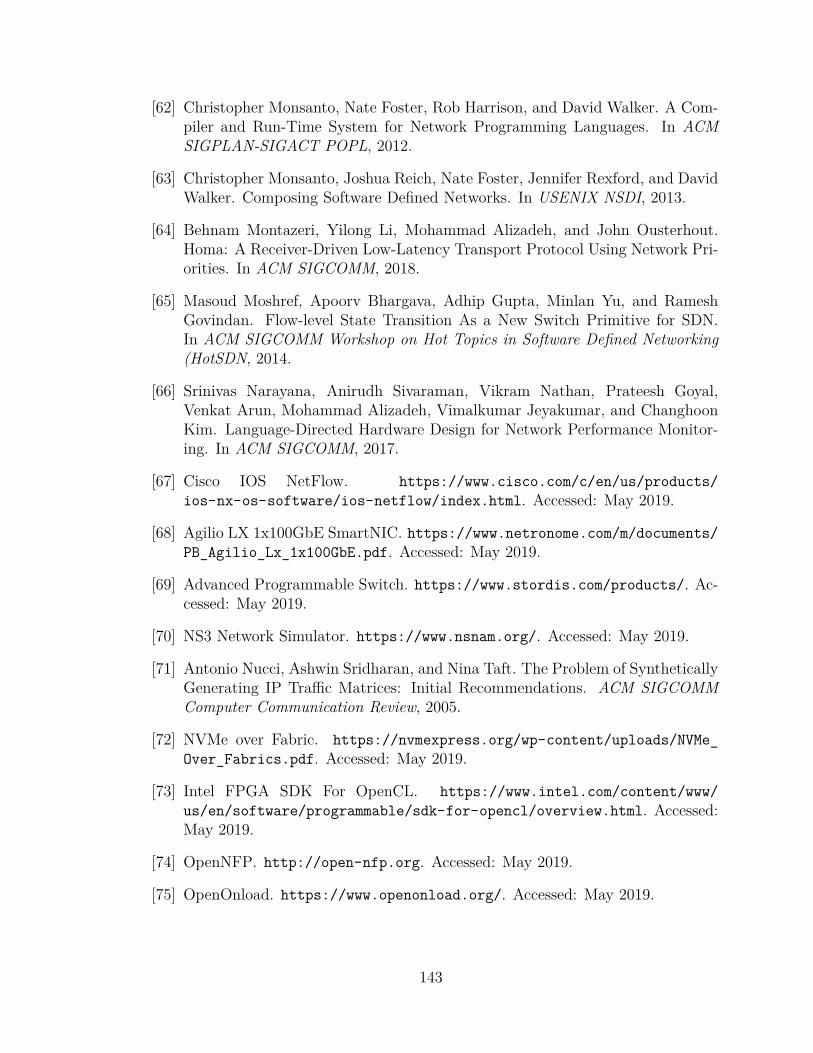
[62] Christopher Monsanto, Nate Foster, Rob Harrison, and David Walker. A Com-piler and Run-Time System for Network Programming Languages. In ACMSIGPLAN-SIGACT POPL, 2012.

[63] Christopher Monsanto, Joshua Reich, Nate Foster, Jennifer Rexford, and DavidWalker. Composing Software Defined Networks. In USENIX NSDI, 2013.

[64] Behnam Montazeri, Yilong Li, Mohammad Alizadeh, and John Ousterhout.Homa: A Receiver-Driven Low-Latency Transport Protocol Using Network Pri-orities. In ACM SIGCOMM, 2018.

[65] Masoud Moshref, Apoorv Bhargava, Adhip Gupta, Minlan Yu, and RameshGovindan. Flow-level State Transition As a New Switch Primitive for SDN.In ACM SIGCOMM Workshop on Hot Topics in Software Defined Networking(HotSDN, 2014.

[66] Srinivas Narayana, Anirudh Sivaraman, Vikram Nathan, Prateesh Goyal,Venkat Arun, Mohammad Alizadeh, Vimalkumar Jeyakumar, and ChanghoonKim. Language-Directed Hardware Design for Network Performance Monitor-ing. In ACM SIGCOMM, 2017.

[67] Cisco IOS NetFlow. https://www.cisco.com/c/en/us/products/ios-nx-os-software/ios-netflow/index.html. Accessed: May 2019.

[68] Agilio LX 1x100GbE SmartNIC. https://www.netronome.com/m/documents/PB_Agilio_Lx_1x100GbE.pdf. Accessed: May 2019.

[69] Advanced Programmable Switch. https://www.stordis.com/products/. Ac-cessed: May 2019.

[70] NS3 Network Simulator. https://www.nsnam.org/. Accessed: May 2019.

[71] Antonio Nucci, Ashwin Sridharan, and Nina Taft. The Problem of SyntheticallyGenerating IP Traffic Matrices: Initial Recommendations. ACM SIGCOMMComputer Communication Review, 2005.

[72] NVMe over Fabric. https://nvmexpress.org/wp-content/uploads/NVMe_Over_Fabrics.pdf. Accessed: May 2019.

[73] Intel FPGA SDK For OpenCL. https://www.intel.com/content/www/us/en/software/programmable/sdk-for-opencl/overview.html. Accessed:May 2019.

[74] OpenNFP. http://open-nfp.org. Accessed: May 2019.

[75] OpenOnload. https://www.openonload.org/. Accessed: May 2019.

143

[76] Chaithan Prakash, Jeongkeun Lee, Yoshio Turner, Joon-Myung Kang, AdityaAkella, Sujata Banerjee, Charles Clark, Yadi Ma, Puneet Sharma, and YingZhang. PGA: Using Graphs to Express and Automatically Reconcile NetworkPolicies. In ACM SIGCOMM, 2015.

[77] Andrew Putnam, Adrian M Caulfield, Eric S Chung, Derek Chiou, Kypros Con-stantinides, John Demme, Hadi Esmaeilzadeh, Jeremy Fowers, Gopi PrashanthGopal, Jan Gray, Michael Haselman, Scott Hauck, Stephen Heil, Amir Hormati,Joo-Young Kim, Sitaram Lanka, James Larus, Eric Peterson, Simon Pope,Aaron Smith, Jason Thong, Phillip Yi Xiao, and Doug Burger. A Reconfig-urable Fabric for Accelerating Large-Scale Datacenter Services. In ISCA, 2014.

[78] PyPy. http://pypy.org. Accessed: May 2019.

[79] Zafar Ayyub Qazi, Cheng-Chun Tu, Luis Chiang, Rui Miao, Vyas Sekar, andMinlan Yu. SIMPLE-fying Middlebox Policy Enforcement Using SDN. In ACMSIGCOMM, 2013.

[80] Bruno Quoitin, Virginie Van den Schrieck, Pierre François, and OlivierBonaventure. IGen: Generation of Router-Level Internet Topologies throughNetwork Design Heuristics. In IEEE International Teletraffic Congress, 2009.

[81] Shriram Rajagopalan, Dan Williams, Hani Jamjoom, and Andrew Warfield.Split/Merge: System Support for Elastic Execution in Virtual Middleboxes. InUSENIX NSDI, 2013.

[82] RoCE Accelerates Data Center Performance, Cost Efficiency, and Scal-ability. http://www.roceinitiative.org/wp-content/uploads/2017/01/RoCE-Accelerates-DC-performance_Final.pdf. Accessed: May 2019.

[83] Matthew Roughan. Simplifying the Synthesis of Internet Traffic Matrices. ACMSIGCOMM Computer Communication Review, 2005.

[84] Arjun Roy, Hongyi Zeng, Jasmeet Bagga, George Porter, and Alex C Snoeren.Inside the Social Network’s (Datacenter) Network. In ACM SIGCOMM, 2015.

[85] Ahmed Saeed, Nandita Dukkipati, Vytautas Valancius, Carlo Contavalli, andAmin Vahdat. Carousel: Scalable Traffic Shaping at End Hosts. In ACMSIGCOMM, 2017.

[86] Jerome H Saltzer, David P Reed, and David D Clark. End-to-End Argumentsin System Design. Technology, 1984.

[87] sFlow. https://sflow.org/. Accessed: May 2019.

[88] Muhammad Shahbaz and Nick Feamster. The Case for an Intermediate Repre-sentation for Programmable Data Planes. In ACM SOSR, 2015.

144

[89] Madhavapeddi Shreedhar and George Varghese. Efficient Fair Queuing UsingDeficit Round-Robin. ACM/IEEE Transactions on Networking, 1996.

[90] Anirudh Sivaraman, Alvin Cheung, Mihai Budiu, Changhoon Kim, Moham-mad Alizadeh, Hari Balakrishnan, George Varghese, Nick McKeown, and SteveLicking. Packet Transactions: High-Level Programming for Line-Rate Switches.In ACM SIGCOMM, 2016.

[91] Anirudh Sivaraman, Suvinay Subramanian, Mohammad Alizadeh, SharadChole, Shang-Tse Chuang, Anurag Agrawal, Hari Balakrishnan, Tom Edsall,Sachin Katti, and Nick McKeown. Programmable Packet Scheduling at LineRate. In ACM SIGCOMM, 2016.

[92] Steffen Smolka, Spiridon Aristides Eliopoulos, Nate Foster, and Arjun Guha.A Fast Compiler for NetKAT. In ACM SIGPLAN ICFP, 2015.

[93] Snort. http://www.snort.org. Accessed: May 2019.

[94] Snort Blog. http://blog.snort.org. Accessed: May 2019.

[95] Robert Soulé, Shrutarshi Basu, Parisa Jalili Marandi, Fernando Pedone, RobertKleinberg, Emin Gun Sirer, and Nate Foster. Merlin: A Language for Provi-sioning Network Resources. In ACM CoNEXT, 2014.

[96] Neil Spring, Ratul Mahajan, David Wetherall, and Thomas Anderson. Measur-ing ISP Topologies with Rocketfuel. IEEE/ACM Transactions on Networking,2004.

[97] Martin Suchara, Dahai Xu, Robert Doverspike, David Johnson, and JenniferRexford. Network Architecture for Joint Failure Recovery and Traffic Engineer-ing. In ACM SIGMETRICS, 2011.

[98] Nik Sultana, Salvator Galea, David Greaves, Marcin Wójcik, Jonny Shipton,Richard Clegg, Luo Mai, Pietro Bressana, Robert Soulé, Richard Mortier, et al.Emu: Rapid Prototyping of Networking Services. In USENIX ATC, 2017.

[99] Mina Tahmasbi Arashloo, Yaron Koral, Michael Greenberg, Jennifer Rexford,and David Walker. SNAP: Stateful Network-Wide Abstractions for PacketProcessing. arXiv preprint arXiv:1512.00822v2, 2015.

[100] Mina Tahmasbi Arashloo, Yaron Koral, Michael Greenberg, Jennifer Rexford,and David Walker. SNAP: Stateful Network-Wide Abstractions for PacketProcessing. In ACM SIGCOMM, 2016.

[101] Mina Tahmasbi Arashloo, Yaron Koral, Michael Greenberg, Jennifer Rexford,and David Walker. SNAP: Stateful Network-Wide Abstractions for PacketProcessing. Technical Report TR-987-16, Department of Computer Science,Princeton University, 2016.

145

[102] Renata Teixeira, Nick Duffield, Jennifer Rexford, and Matthew Roughan. Traf-fic Matrix Reloaded: Impact of Routing Changes. In Passive and Active Net-work Measurement. 2005.

[103] Tofino, World’s Fastest P4-Programmable Ethernet Switch ASICs. https://www.barefootnetworks.com/products/brief-tofino/. Accessed: May 2019.

[104] Christo Wilson, Hitesh Ballani, Thomas Karagiannis, and Ant Rowtron. Bet-ter Never than Late: Meeting Deadlines in Datacenter Networks. In ACMSIGCOMM, 2011.

[105] Vivado High-Level Synthesis. https://www.xilinx.com/products/design-tools/vivado/integration/esl-design.html. Accessed: May2019.

[106] Cavium XPliant Ethernet Switch Product Line. https://www.marvell.com/documents/netpxrx94dcdhk8sksbp/. Accessed: May 2019.

[107] Minlan Yu, Lavanya Jose, and Rui Miao. Software Defined Traffic Measurementwith OpenSketch. In USENIX NSDI, 2013.

[108] Yifei Yuan, Rajeev Alur, and Boon Thau Loo. NetEgg: Programming Net-work Policies by Examples. In ACM SIGCOMM Workshop on Hot Topics inNetworks (HotNets), 2014.

[109] Yibo Zhu, Haggai Eran, Daniel Firestone, Chuanxiong Guo, Marina Lipshteyn,Yehonatan Liron, Jitendra Padhye, Shachar Raindel, Mohamad Haj Yahia, andMing Zhang. Congestion Control for Large-Scale RDMA Deployments. In ACMSIGCOMM, 2015.

[110] Yibo Zhu, Monia Ghobadi, Vishal Misra, and Jitendra Padhye. ECN or Delay:Lessons Learnt from Analysis of DCQCN and TIMELY. In ACM CoNEXT,2016.

146