State-Space Models with EndogenousMarkov Regime Switching Parameters

Kyu Ho Kang∗

(Department of Economics, Washington University in St. Louis, Box 1208, MO 63130, USA)

This Version: July 2010

Abstract

In this paper, Kim, Piger and Startz’ (2008) endogenous Markov-switchingmodel is extended to a general state-space model. This paper also complementsKim’s (1991) regime switching dynamic linear models by allowing the discreteregime to be jointly determined with observed or unobserved continuous statevariables. An efficient Bayesian MCMC estimation method is developed. It isshown that simulation of the latent state variable controlling the regime shiftsenables us to precisely estimate the models without approximation. This methodis applied to the estimation of a generalized Nelson-Siegel yield curve model wherethe unobserved time-varying curvature factor is allowed to be contemporaneouslycorrelated with Markov switching volatility regimes. All techniques are also illus-trated using simulated data sets. (JEL classification: C1; C4)

Keywords : Bayesian estimation, Markov switching process, Markov Chain MonteCarlo, Bayes factor, Term structure of interest rates

1 Introduction

State-space models with regime switching parameters are so flexible that they have been

commonly used to model heterogenous dynamics of data over time (For instance, Kim

(1994), Kim and Piger (2002) and Kuan, Huang, and Tsay (2005)). The flexibility of

this modeling approach is due to the fact that it involves two different types of dynamic

state variables. One is usually termed as a regime indicator and it takes on discrete

values determining the set of state-contingent model parameters at each data point.

∗Email : khkang@wustl.edu

1

The other is generated from continuous probability distributions over time (for example,

ARMA process) and responsible for the dynamics within the discrete state. Those state

variables are both responsible for the dynamics of observed quantities. In modeling

with such dynamic systems, it is essential to consider contemporaneous feedback among

the state variables in many empirical works. The instantaneous interaction between

continuous state variables can be modeled by allowing for non-zero correlation of the

innovations. (For instance, Morley, Nelson, and Zivot (2003)). Also by estimating the

full transition matrix one can consider the co-movement of discrete state variables (i.e.

regime indicators).

Although this modeling strategy is convenient and useful in many applications, it

is rather restrictive because it only permits instantaneous interaction among the state

variables with the same type. A more general approach is to allow for the bi-directional

feedback between the two different types of the underlying state variables. In particular,

this general approach, which has not been addressed yet, may be important in many

macroeconomics or finance models. For example, in Nelson-Siegel yield curve models,

the slope and curvature of the term structure, which are modeled as unobserved factors,

affect the future risk premia (Cochrane and Piazzesi (2008)). Also they are highly likely

to be contemporaneously correlated with Markov switching volatility regimes since the

size of shock volatilities determines the magnitude of the risk. It thus seems more sensible

to model the joint realization of those two different types of unobserved underlying

stochastic processes.

The purpose of this paper is to develop and estimate state space models in which

the unobserved discrete regimes and continuous state variables are jointly determined.

The regime switches are modeled through a Markov process. In this model formulation,

it becomes possible to make the realization of the regimes endogenized through the

correlation with the observed or unobserved continuous state variables. Our statistical

inference is fully Bayesian. The MCMC method developed by this paper builds on the

works of Albert and Chib (1993) and Kim, Piger, and Startz (2008). Kim et al. (2008)

propose endogenous Markov-switching linear models which do not involve the dynamics

of continuous state variables, and our work extends their work to a general state-space

2

model. We show that it can be done by introducing and simulating the latent state

variables that control regime shifts at each time point. This idea of data augmentation

is based on the work of Albert and Chib (1993), in which exact Bayesian methods for

modeling categorical response data are developed.1 In addition, we conduct a Bayesian

model choice between endogenous switching and exogenous switching model based on

the marginal likelihoods.

In the next section, we lay out a two-regime Markov-switching dynamic factor model

with endogenous switching. Section 3 discusses our Bayesian MCMC estimation method.

Section 4 gives the results of simulation study and an empirical work. Section 5 has the

conclusion.

2 The Class of Models

We study a class of state-space models where at each time point the model parameters

are chosen by a discrete state Markov process indexed by st, and some of the unobserved

factors and the state variable are contemporaneously correlated. The models we discuss

are represented by a state space form,

yt = ast + bstft + Hstxt + Dstet, et ∼ i.i.d.Nq(0, Iq) (2.1)

ft = µst + Gstft−1 + Lεt, εt ∼ i.i.d.Nk(0, Ik) (2.2)

where yt is a q-dimensional vector of dependent variables with finite first and second

moments and ft is a k-dimensional vector of observed or unobserved continuous state

variables. xt is a h-dimensional vector of the observed exogenous or predetermined

variables, and it is assumed to be covariance-stationary. ast , bst and Hst are q×1, q×kand q×h matrices, respectively. µst : k×1 and Gst : k×k determine the state-dependent

mean and persistence of the factors. Dst : q × q and L : k × k capture the volatilities

of the measurement errors and the continuous state shocks. In addition, et and εt are

assumed to be mutually independent, and E [et|Sn] = 0 and E [ete′t|Sn] = Iq.

1Chib and Dueker (2004), as one of related works in the Bayesian approach, develop a non-Markovianregime switching model. In their setup, the regime states depend on the sign of an autoregressive latentvariable, which is allowed to be endogenous in sense that regimes are determined jointly with theobserved data.

3

In what follows, we postulate that the number of regimes is two as in Hamilton

(1989). The two-regime case is not only convenient to explain and understand, but also

popular in many empirical studies. We also assume that the unobserved discrete state

variable st is governed by a first-order Markov chain with transition probabilities:

p(st = k|st−1 = j, zt) = pjk(zt) (2.3)

where zt is a vector of covariance-stationary exogenous or predetermined variables, which

may include some elements of xt. (i.e. the regime-switching point positions are modeled

as a Markov process.) The Markov chain is assumed to be stationary and independent of

all observations of those elements of xt not included in zt. For the purpose a convenient

formulation of the Markov process, we introduce another latent variable γt, so that the

influence of zt on the transition probabilities is modeled through a probit specification

as in Kim et al. (2008).

st =

1 if γt < αst−1 + β′st−1

zt2 if γt > αst−1 + β′st−1

ztwhere γt ∼ i.i.d.N (0, 1) (2.4)

In other words. the transition probabilities have the form

pj1(zt) = Pr[γt < αj + β′jzt

]= Φ

(αj + β′jzt

)(2.5)

pj2(zt) = 1− Φ(αj + β′jzt

)By allowing for non-zero correlation between the regime shock γt and the factor shock

εt we model a bi-directional contemporaneous feedback between the unobserved state

variable st and the unobserved factors ft[εtγt

]∼ i.i.d.Nk+1

(0(k+1)×1,

(Ik ρρ′ 1

))(2.6)

where ρ =(ρ1 ρ2 · · · ρk

)′. Hence, the presence of some none-zero ρ′is (i = 1, 2, .., k)

implies endogenous regime changes, and the realization of regime at the next period

is determined jointly with the vector of continuous latent (or observable) variables.

This feature distinguishes our work from the existing studies. For example, when all

ρ′is are zero, we have the Markov switching dynamic factor model with time-varying

transition probability of Kim and Nelson (1998). Also it is very useful to notice that

4

when k = q = bst = 1 and Gst = µst = Dst = 0, this class of models reduces to that

of Kim et al. (2008) in which yt is scalar and thereby no unobserved continuous state

variable is involved.

Many other interesting models can also be constructed as special cases such as time-

varying coefficient model, dynamic common factor model and unobserved component

model and so forth. Specifically, one may set yt as a vector of stationary asset returns

and ft as the dynamic common factors where the factor loadings are regime-specific. So

yt may endogenously switch between strong and weak co-movement among the observed

returns over time. It is also possible to specify and evaluate the endogenous asymmetry

in the business cycle using the Friedman’s plucking model context.2

st+1stst−1

ft−1 ft+1ft

Θst−1Θst+1Θst

yt−1 yt+1yt.

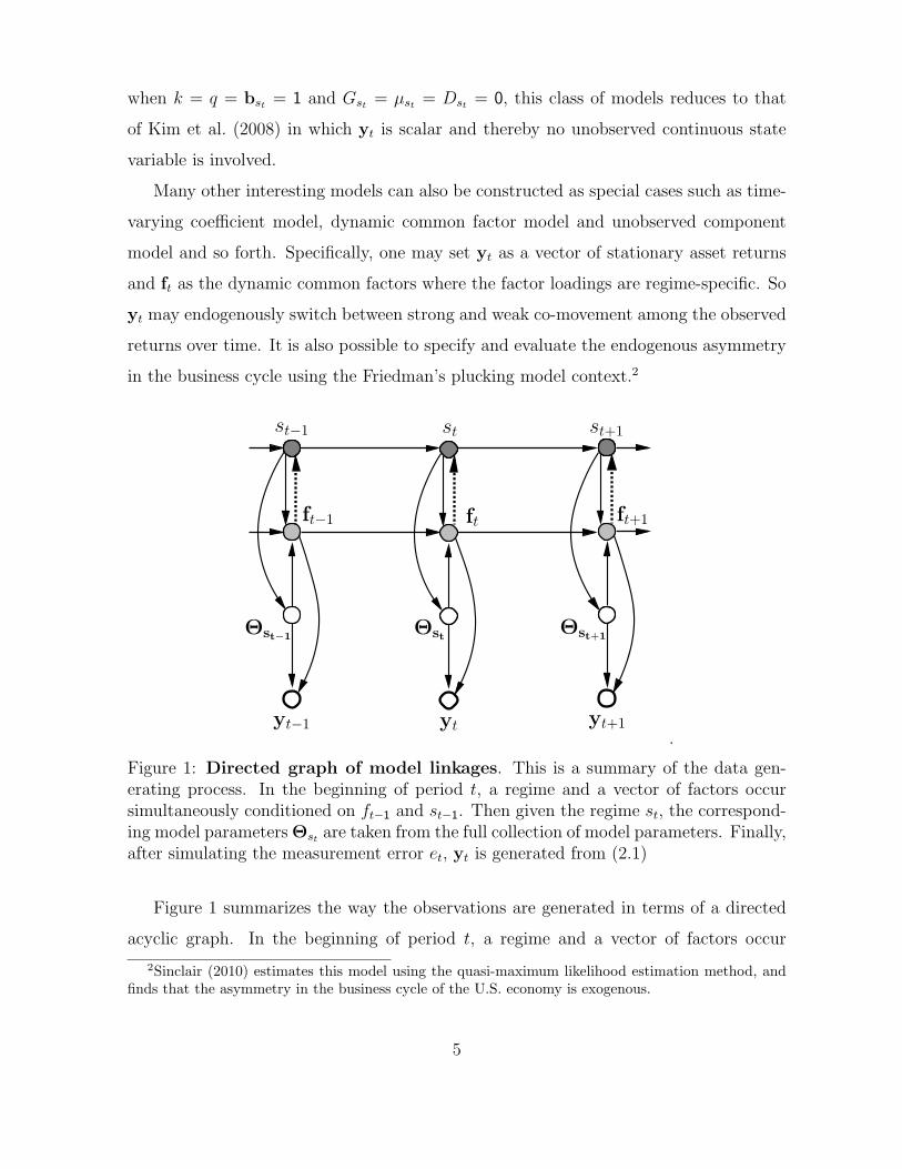
Figure 1: Directed graph of model linkages. This is a summary of the data gen-erating process. In the beginning of period t, a regime and a vector of factors occursimultaneously conditioned on ft−1 and st−1. Then given the regime st, the correspond-ing model parameters Θst are taken from the full collection of model parameters. Finally,after simulating the measurement error et, yt is generated from (2.1)

Figure 1 summarizes the way the observations are generated in terms of a directed

acyclic graph. In the beginning of period t, a regime and a vector of factors occur

2Sinclair (2010) estimates this model using the quasi-maximum likelihood estimation method, andfinds that the asymmetry in the business cycle of the U.S. economy is exogenous.

5

simultaneously. This realization of the regime at time t is governed with the regime in

the previous period and the current factors as indicated by the direction of the two arrows

connecting st−1 to st and ft to st. Then given the regime at time t, the corresponding

model parameters Θst are taken from the full collection of model parameters. These

include ast and bst , for example. Conditioned on the parameters and ft−1, ft is generated

by the regime-specific autoregressive process in (2.2). Finally, from (2.1), ast , bst , ft

and a simulated measurement error et at each time point construct the observations yt.

Notice that in standard state space models with regime switching parameters the dashed

line in figure 1 is absent since st is assumed to be drawn independently of ft.

3 Prior-Posterior Analysis

3.1 Markov Chain Monte Carlo Scheme

Let Yt = yii=1,2,..,t, Xt = xii=1,2,..,t and Zt = zii=1,2,..,t be observations observed

through time t. Similarly, Ft = fii=1,2,..,t, St = sii=1,2,..,t and γt = γii=1,2,..,t

denote collection of the state variables through time t. Let Θ denote the parameters

in the evolution and transition equations and P is those in the transition probabili-

ties. That is, Θ is the collection of the parameters in ast ,bst ,Hst ,Dst ,µst ,Gst ,Lst and

P =α1,α2,β′1,β′2,ρ1,ρ2,..,ρk. Suppose that we have specified a prior density π(Θ,P) on

the parameters and data Yn, Zn and Xn are available. A Bayesian state space model

with regime switching parameters is defined by a joint distribution over the regime states,

continuous latent variables, model parameters and the data. In this context, interest

centers on the posterior density π (Θ,P,Sn,γn,Fn|Yn,Ωn), and

π (Θ,P,Sn,γn,Fn|Yn,Ωn) (3.1)

∝ f (Yn|Ωn,Sn,γn,Fn,Θ,P)× p (Sn,γn,Fn|Ωn,Θ,P)× π(Θ,P)

where Ωt = Xt ∪ Zt is the collection of exogenous variables at time t whose dynamics

are not analyzed through the transition equation in equation (2.2). Note that we use

the notation π to denote prior and posterior density functions of (Θ,P). We apply our

MCMC sampling scheme to the posterior density π (Θ,P,Sn,γn,Fn|Yn,Ωn) and obtain

6

the posterior distribution π (Θ,P|Yn,Ωn) by integrating out (Sn,γn,Fn) in a numerical

way.

We sample the parameters and the states recursively. In the first step, the parameters

in Θ are simulated on (Sn,Ωn,Wn,P,γn) and then P is sampled in turn. Next, the states

Sn are drawn conditioned on (Wn,Ωn) and the other parameters where Wt = Yt ∪Ft.

Then we sequentially simulate γn and Fn conditioned on the most recent values of the

conditioning variables. Our MCMC algorithm can be summarized as follows.

Algorithm: MCMC sampling

Step 1 Initialize (Sn,Fn,P,γn) and fix n0 (the burn-in) and n1 (the MCMC sample

size)

Step 2 Sample Θ|Wn,Ωn,Sn,γn,P

Step 3 Sample P|Wn,Ωn,Sn,Θ

Step 4 Sample Sn|Wn,Ωn,Θ,P

Step 5 Sample γn|Wn,Ωn,Sn,Θ,P

Step 6 Sample Fn|Yn,Ωn,Sn,γn,Θ,P

Step 7 Repeat Steps 2-6, discard the draws from the first n0 iterations and save the

subsequent n1 draws.

Full details of each of these steps are given by the following.

3.1.1 Simulation of Θ

We consider the question of simulating Θ conditioned on (Ωn,Wn,Sn,γn,P) by the

tailored multiple block MH algorithm(Chib and Greenberg (1995)). In this method the

parameters in Θ are first blocked into various sub-blocks. Then each of these sub-blocks

is sampled in sequence by drawing a value from a tailored proposal density constructed

for that particular block. This proposal is then accepted or rejected by the usual MH

7

probability move. For instance, suppose that in the jth iteration, we have g sub-blocks

of Θ

Θ1, Θ2, . ., Θg

Then the proposal density q(Θi|Θ−i,Wn,γn,Sn,P

)for the ith block, conditioned on

the most current value of the remaining blocks Θ−i, is constructed by a quadratic ap-

proximation at the mode of the current target density π(Θi|Θ−i,Wn,γn,Sn,P

). In

our case, we let this proposal density take the form of a student t distribution with 15

degrees of freedom

q(Θi|Θ−i,P,Wn,γn,Ωn,Sn

)= St (Θi|Θi,P,VΘi

,15) (3.2)

where

Θi = arg maxΘi

lnf(Wn|γn,Ωn,Sn,Θi,Θ−i,P)π(Θi) (3.3)

and VΘi=

(−∂

2 lnf(Wn|γn,Ωn,Sn,Θi,Θ−i,P)π(Θi)

∂Θi∂Θ′i

)−1

|Θi=Θi

.

We then generate a proposal value Θ†i . If Θ†i violates any of the constraints in R,

it is immediately rejected. Otherwise, it is accepted as the next value in the chain with

probability

α(Θ

(j−1)i ,Θ†i |Θ−i

)(3.4)

= min

f(Wn|γn,Ωn,Sn,Θ†i ,Θ−i,P)π

(Θ†i

)f(Wn|γn,Ωn,Sn,Θ

(j−1)i ,Θ−i,P

)π(Θ

(j−1)i

) St(Θ

(j−1)i |Θi,P,VΘi

,15)

St(Θ†i |Θi,P,VΘi

,15) , 1

.

The simulation of Θ is complete when all the sub-blocks Θii=1,2,..,g are sequentially

updated as above. On letting Nq (x|a, b) denote the q-dimensional multivariate nor-

mal density of x with mean of a and variance of b, the required joint density of Wn

conditioned on (Ωn,γn,Sn,Θ,P) is then a product of conditional predictive densities:

f (Wn|γn,Ωn,Sn,Θ,P) (3.5)

=n∏t=1

Nq(yt|yt|t−1, DstD

′st

)×Nk

(ft|ft|t−1, Lst (Ik − ρρ′)L′st

)8

where

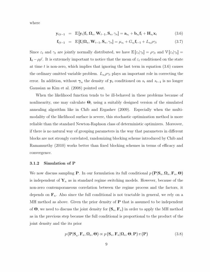
yt|t−1 = E [yt|ft,Ωn,Wt−1,Sn, γn] = ast + bstft + Hstxt (3.6)

ft|t−1 = E [ft|Ωn,Wt−1,Sn, γn] = µst + Gstft−1 + Lstργt (3.7)

Since εt and γt are jointly normally distributed, we have E [εt|γt] = ργt and V [εt|γt] =

Ik−ρρ′. It is extremely important to notice that the mean of εt conditioned on the state

at time t is non-zero, which implies that ignoring the last term in equation (3.6) causes

the ordinary omitted variable problem. Lstργt plays an important role in correcting the

error. In addition, without γn the density of yt conditioned on st and st−1 is no longer

Gaussian as Kim et al. (2008) pointed out.

When the likelihood function tends to be ill-behaved in these problems because of

nonlinearity, one may calculate Θi using a suitably designed version of the simulated

annealing algorithm like in Chib and Ergashev (2009). Especially when the multi-

modality of the likelihood surface is severe, this stochastic optimization method is more

reliable than the standard Newton-Raphson class of deterministic optimizers. Moreover,

if there is no natural way of grouping parameters in the way that parameters in different

blocks are not strongly correlated, randomizing blocking scheme introduced by Chib and

Ramamurthy (2010) works better than fixed blocking schemes in terms of efficacy and

convergence.

3.1.2 Simulation of P

We now discuss sampling P. In our formulation its full conditional p (P|Sn,Ωn,Fn,Θ)

is independent of Yn as in standard regime switching models. However, because of the

non-zero contemporaneous correlation between the regime process and the factors, it

depends on Fn. Also since the full conditional is not tractable in general, we rely on a

MH method as above. Given the prior density of P that is assumed to be independent

of Θ, we need to discuss the joint density for (Sn,Fn) in order to apply the MH method

as in the previous step because the full conditional is proportional to the product of the

joint density and the its prior

p (P|Sn,Fn,Ωn,Θ) ∝ p (Sn,Fn|Ωn,Θ,P)π (P) (3.8)

9

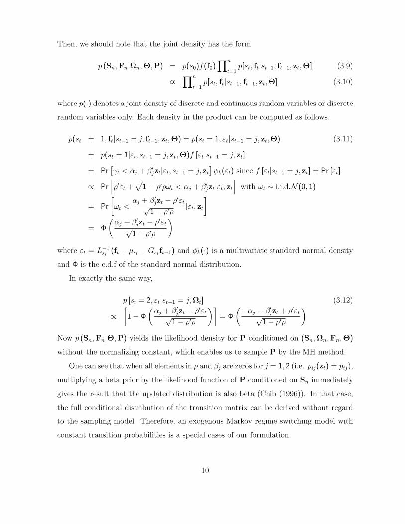
Then, we should note that the joint density has the form

p (Sn,Fn|Ωn,Θ,P) = p(s0)f(f0)∏n

t=1p[st, ft|st−1, ft−1, zt,Θ] (3.9)

∝∏n

t=1p[st, ft|st−1, ft−1, zt,Θ] (3.10)

where p(·) denotes a joint density of discrete and continuous random variables or discrete

random variables only. Each density in the product can be computed as follows.

p(st = 1, ft|st−1 = j, ft−1, zt,Θ) = p(st = 1, εt|st−1 = j, zt,Θ) (3.11)

= p(st = 1|εt, st−1 = j, zt,Θ)f [εt|st−1 = j, zt]

= Pr[γt < αj + β′jzt|εt, st−1 = j, zt

]φk(εt) since f [εt|st−1 = j, zt] = Pr [εt]

∝ Pr[ρ′εt +

√1− ρ′ρωt < αj + β′jzt|εt, zt

]with ωt ∼ i.i.d.N (0, 1)

= Pr

[ωt <

αj + β′jzt − ρ′εt√1− ρ′ρ |εt, zt

]= Φ

(αj + β′jzt − ρ′εt√

1− ρ′ρ

)where εt = L−1

st (ft − µst −Gstft−1) and φk(·) is a multivariate standard normal density

and Φ is the c.d.f of the standard normal distribution.

In exactly the same way,

p [st = 2, εt|st−1 = j,Ωt] (3.12)

∝[

1− Φ

(αj + β′jzt − ρ′εt√

1− ρ′ρ

)]= Φ

(−αj − β′jzt + ρ′εt√1− ρ′ρ

)Now p (Sn,Fn|Θ,P) yields the likelihood density for P conditioned on (Sn,Ωn,Fn,Θ)

without the normalizing constant, which enables us to sample P by the MH method.

One can see that when all elements in ρ and βj are zeros for j = 1, 2 (i.e. pij(zt) = pij),

multiplying a beta prior by the likelihood function of P conditioned on Sn immediately

gives the result that the updated distribution is also beta (Chib (1996)). In that case,

the full conditional distribution of the transition matrix can be derived without regard

to the sampling model. Therefore, an exogenous Markov regime switching model with

constant transition probabilities is a special cases of our formulation.

10

3.1.3 Simulation of st

In order to sample Sn we provide a generalized version of the method of Chib (1996),

where exogenous Markov mixture models are analyzed by MCMC methods. The ob-

jective in this subsection is to draw a sequence of values of stt=0,1,2,..,n jointly from

p(Sn|Wn,Ωn,Θ,P) where the state process is endogenous. It can be easily seen that

this sampling is simulating st from p (st|Wn,Ωn, st+1,Θ,P), and by Bayes theorem

p (st|Wn,Ωn, st+1,Θ,P) ∝ p (st|Wt,Ωt,Θ,P) p (st+1|st,Ωt+1, ft+1,Θ,P) (3.13)

In this approach, the sampling of Sn is achieved by one forward and backward pass

through the data.

In the forward pass, one recursively obtains the sequence of filtered probabilities

p (st|Wn,Ωn,Θ,P) by calculating

p (st|Wt,Ωt,Θ,P) (3.14)

=

∑2j=1 f (yt, ft|Wt−1, st−1 = j, st,Ωt,Θ,P) p (st−1 = j, st|Ωt,Θ,P)

f (yt, ft|Wt−1,Ωt,Θ,P)(3.15)

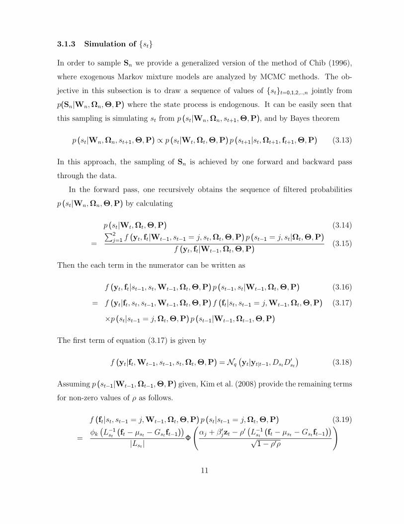
Then the each term in the numerator can be written as

f (yt, ft|st−1, st,Wt−1,Ωt,Θ,P) p (st−1, st|Wt−1,Ωt,Θ,P) (3.16)

= f (yt|ft, st, st−1,Wt−1,Ωt,Θ,P) f (ft|st, st−1 = j,Wt−1,Ωt,Θ,P) (3.17)

×p (st|st−1 = j,Ωt,Θ,P) p (st−1|Wt−1,Ωt−1,Θ,P)

The first term of equation (3.17) is given by

f (yt|ft,Wt−1, st−1, st,Ωt,Θ,P) = Nq(yt|yt|t−1, DstD

′st

)(3.18)

Assuming p (st−1|Wt−1,Ωt−1,Θ,P) given, Kim et al. (2008) provide the remaining terms

for non-zero values of ρ as follows.

f (ft|st, st−1 = j,Wt−1,Ωt,Θ,P) p (st|st−1 = j,Ωt,Θ,P) (3.19)

=φk(L−1st (ft − µst −Gstft−1)

)|Lst |

Φ

(αj + β′jzt − ρ′

(L−1st (ft − µst −Gstft−1)

)√

1− ρ′ρ

)

11

These calculations are initialized at t = 1 by treating the initial probability p (s0|W0,Ω0,Θ,P)

as an additional parameter to be estimated or approximating it by the unconditional

probability p (s0|,Θ,P). With the numerator at hand, the conditional joint density of yt

and ft which is the denominator of equation (3.14) is given by the law of total probability

f (yt, ft|Wt−1,Ωt,Θ,P) (3.20)

=2∑

st=1

2∑st−1=1

f (yt, ft|st−1, st,Wt−1,Ωt,Θ,P) p (st−1, st|Wt−1,Ωt,Θ,P)

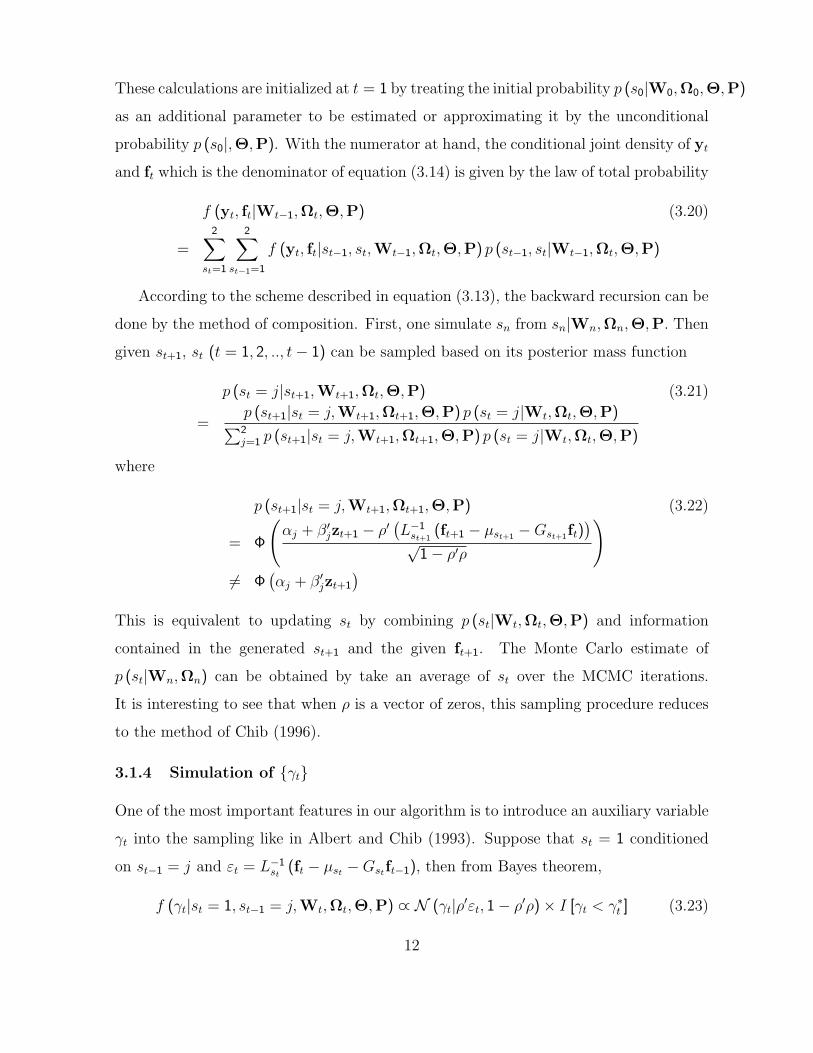
According to the scheme described in equation (3.13), the backward recursion can be

done by the method of composition. First, one simulate sn from sn|Wn,Ωn,Θ,P. Then

given st+1, st (t = 1, 2, .., t− 1) can be sampled based on its posterior mass function

p (st = j|st+1,Wt+1,Ωt,Θ,P) (3.21)

=p (st+1|st = j,Wt+1,Ωt+1,Θ,P) p (st = j|Wt,Ωt,Θ,P)∑2j=1 p (st+1|st = j,Wt+1,Ωt+1,Θ,P) p (st = j|Wt,Ωt,Θ,P)

where

p (st+1|st = j,Wt+1,Ωt+1,Θ,P) (3.22)

= Φ

(αj + β′jzt+1 − ρ′

(L−1st+1

(ft+1 − µst+1 −Gst+1ft))

√1− ρ′ρ

)6= Φ

(αj + β′jzt+1

)This is equivalent to updating st by combining p (st|Wt,Ωt,Θ,P) and information

contained in the generated st+1 and the given ft+1. The Monte Carlo estimate of

p (st|Wn,Ωn) can be obtained by take an average of st over the MCMC iterations.

It is interesting to see that when ρ is a vector of zeros, this sampling procedure reduces

to the method of Chib (1996).

3.1.4 Simulation of γt

One of the most important features in our algorithm is to introduce an auxiliary variable

γt into the sampling like in Albert and Chib (1993). Suppose that st = 1 conditioned

on st−1 = j and εt = L−1st (ft − µst −Gstft−1), then from Bayes theorem,

f (γt|st = 1, st−1 = j,Wt,Ωt,Θ,P) ∝ N (γt|ρ′εt, 1− ρ′ρ)× I [γt < γ∗t ] (3.23)

12

where γ∗t = αj + β′jzt and I [·] is an indicator function. The information st = 1 simply

serves to truncate the support of γt, which depends on εt due to the correlation. By

a similar agrement, the support of γt is (γ∗t ,∞) conditioned on the event st = 2 and

st−1 = j. Each of these truncated normal distributions is simulated as follows.

γt|εt, st = 1, st−1 = j ∼ T N (−∞,γ∗t ](ρ′εt, 1− ρ′ρ) (3.24)

γt|εt, st = 2, st−1 = j ∼ T N (γ∗t ,∞)(ρ′εt, 1− ρ′ρ)

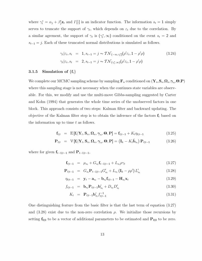
3.1.5 Simulation of ft

We complete our MCMC sampling scheme by sampling Fn conditioned on (Yn,Sn,Ωn,γn,Θ,P)

where this sampling stage is not necessary when the continues state variables are observ-

able. For this, we modify and use the multi-move Gibbs-sampling suggested by Carter

and Kohn (1994) that generates the whole time series of the unobserved factors in one

block. This approach consists of two steps: Kalman filter and backward updating. The

objective of the Kalman filter step is to obtain the inference of the factors ft based on

the information up to time t as follows.

ft|t = E [ft|Yt,Sn,Ωn,γn,Θ,P] = ft|t−1 + Ktηt|t−1 (3.25)

Pt|t = V [ft|Yt,Sn,Ωn,γn,Θ,P] =(Ik −Ktbst

)Pt|t−1 (3.26)

where for given ft−1|t−1 and Pt−1|t−1,

ft|t−1 = µst + Gstft−1|t−1 + Lstργt (3.27)

Pt|t−1 = GstPt−1|t−1G′st + Lst (Ik − ρρ′)L′st (3.28)

ηt|t−1 = yt − ast − bstft|t−1 −Hstxt (3.29)

ft|t−1 = bstPt|t−1b′st + DstD

′st (3.30)

Kt = Pt|t−1b′stf−1t|t−1 (3.31)

One distinguishing feature from the basic filter is that the last term of equation (3.27)

and (3.28) exist due to the non-zero correlation ρ. We initialize those recursions by

setting f0|0 to be a vector of additional parameters to be estimated and P0|0 to be zero.

13

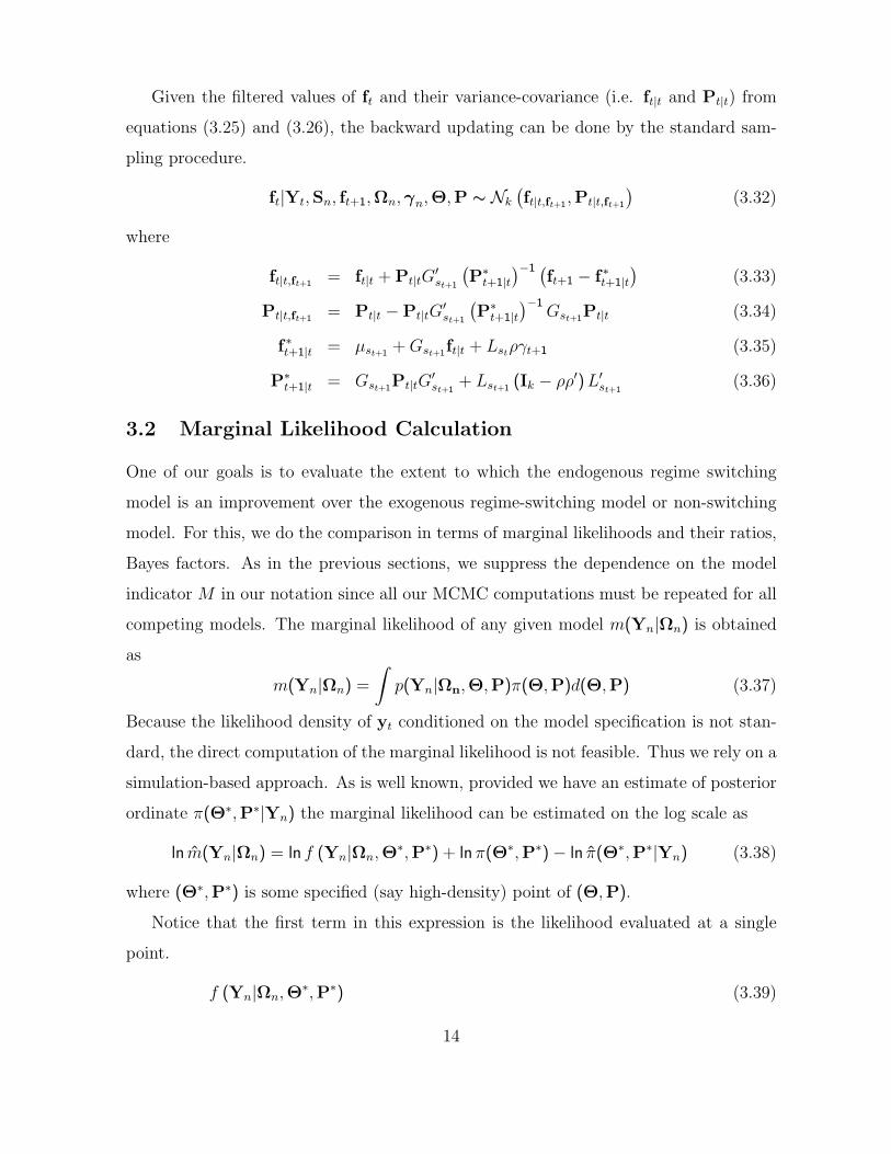
Given the filtered values of ft and their variance-covariance (i.e. ft|t and Pt|t) from

equations (3.25) and (3.26), the backward updating can be done by the standard sam-

pling procedure.

ft|Yt,Sn, ft+1,Ωn,γn,Θ,P ∼ Nk(ft|t,ft+1

,Pt|t,ft+1

)(3.32)

where

ft|t,ft+1= ft|t + Pt|tG

′st+1

(P∗t+1|t

)−1 (ft+1 − f∗t+1|t

)(3.33)

Pt|t,ft+1= Pt|t −Pt|tG

′st+1

(P∗t+1|t

)−1Gst+1Pt|t (3.34)

f∗t+1|t = µst+1 + Gst+1ft|t + Lstργt+1 (3.35)

P∗t+1|t = Gst+1Pt|tG′st+1

+ Lst+1 (Ik − ρρ′)L′st+1(3.36)

3.2 Marginal Likelihood Calculation

One of our goals is to evaluate the extent to which the endogenous regime switching

model is an improvement over the exogenous regime-switching model or non-switching

model. For this, we do the comparison in terms of marginal likelihoods and their ratios,

Bayes factors. As in the previous sections, we suppress the dependence on the model

indicator M in our notation since all our MCMC computations must be repeated for all

competing models. The marginal likelihood of any given model m(Yn|Ωn) is obtained

as

m(Yn|Ωn) =

∫p(Yn|Ωn,Θ,P)π(Θ,P)d(Θ,P) (3.37)

Because the likelihood density of yt conditioned on the model specification is not stan-

dard, the direct computation of the marginal likelihood is not feasible. Thus we rely on a

simulation-based approach. As is well known, provided we have an estimate of posterior

ordinate π(Θ∗,P∗|Yn) the marginal likelihood can be estimated on the log scale as

ln m(Yn|Ωn) = ln f (Yn|Ωn,Θ∗,P∗) + ln π(Θ∗,P∗)− ln π(Θ∗,P∗|Yn) (3.38)

where (Θ∗,P∗) is some specified (say high-density) point of (Θ,P).

Notice that the first term in this expression is the likelihood evaluated at a single

point.

f (Yn|Ωn,Θ∗,P∗) (3.39)

14

=

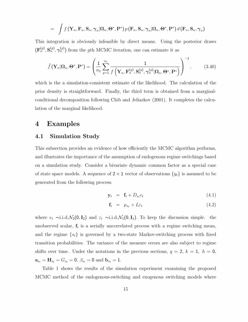
∫f (Yn,Fn,Sn,γn|Ωn,Θ

∗,P∗) p (Fn,Sn,γn|Ωn,Θ∗,P∗) d (Fn,Sn,γn)

This integration is obviously infeasible by direct means. Using the posterior draws

(F(g)n ,S

(g)n ,γ

(g)n ) from the gth MCMC iteration, one can estimate it as

f (Yn|Ωn,Θ∗,P∗) =

1

n1

n1∑g=1

1

f(Yn,F

(g)n ,S

(g)n ,γ

(g)n |Ωn,Θ∗,P∗

)−1

, (3.40)

which is the a simulation-consistent estimate of the likelihood. The calculation of the

prior density is straightforward. Finally, the third term is obtained from a marginal-

conditional decomposition following Chib and Jeliazkov (2001). It completes the calcu-

lation of the marginal likelihood.

4 Examples

4.1 Simulation Study

This subsection provides an evidence of how efficiently the MCMC algorithm performs,

and illustrates the importance of the assumption of endogenous regime switchings based

on a simulation study. Consider a bivariate dynamic common factor as a special case

of state space models. A sequence of 2× 1 vector of observations yt is assumed to be

generated from the following process.

yt = ft + Dstet (4.1)

ft = µst + Lεt (4.2)

where et ∼i.i.d.N2(0, I2) and εt ∼i.i.d.N1(0, I1). To keep the discussion simple. the

unobserved scalar, ft is a serially uncorrelated process with a regime switching mean,

and the regime st is governed by a two-state Markov-switching process with fixed

transition probabilities. The variance of the measure errors are also subject to regime

shifts over time. Under the notations in the previous sections, q = 2, k = 1, h = 0,

ast = Hst = Gst = 0, βst = 0 and bst = 1.

Table 1 shows the results of the simulation experiment examining the proposed

MCMC method of the endogenous-switching and exogenous switching models where

15

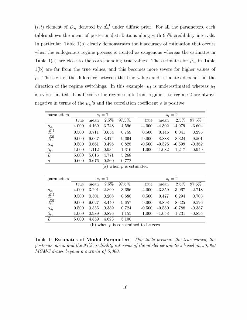
(i, i) element of Dst denoted by d(i)st under diffuse prior. For all the parameters, each

tables shows the mean of posterior distributions along with 95% credibility intervals.

In particular, Table 1(b) clearly demonstrates the inaccuracy of estimation that occurs

when the endogenous regime process is treated as exogenous whereas the estimates in

Table 1(a) are close to the corresponding true values. The estimates for µst in Table

1(b) are far from the true values, and this becomes more severe for higher values of

ρ. The sign of the difference between the true values and estimates depends on the

direction of the regime switchings. In this example, µ1 is underestimated whereas µ2

is overestimated. It is because the regime shifts from regime 1 to regime 2 are always

negative in terms of the µst ’s and the correlation coefficient ρ is positive.

parameters st = 1 st = 2true mean 2.5% 97.5%. true mean 2.5% 97.5%.

µst 4.000 4.169 3.748 4.596 -4.000 -4.302 -4.979 -3.604d

(1)st 0.500 0.711 0.654 0.759 0.500 0.146 0.041 0.295d

(2)st 9.000 9.067 8.474 9.664 9.000 8.888 8.324 9.501αst 0.500 0.661 0.498 0.828 -0.500 -0.526 -0.699 -0.362βst 1.000 1.112 0.934 1.316 -1.000 -1.082 -1.217 -0.949L 5.000 5.016 4.771 5.268ρ 0.600 0.676 0.560 0.772

(a) when ρ is estimated

parameters st = 1 st = 2true mean 2.5% 97.5%. true mean 2.5% 97.5%.

µst 4.000 3.291 2.899 3.696 -4.000 -3.359 -3.967 -2.718d

(1)st 0.500 0.501 0.208 0.680 0.500 0.477 0.294 0.703d

(2)st 9.000 9.027 8.440 9.657 9.000 8.898 8.325 9.526αst 0.500 0.555 0.389 0.724 -0.500 -0.580 -0.788 -0.387βst 1.000 0.989 0.826 1.155 -1.000 -1.058 -1.231 -0.895L 5.000 4.859 4.623 5.100

(b) when ρ is constrained to be zero

Table 1: Estimates of Model Parameters This table presents the true values, theposterior mean and the 95% credibility intervals of the model parameters based on 50,000MCMC draws beyond a burn-in of 5,000.

16

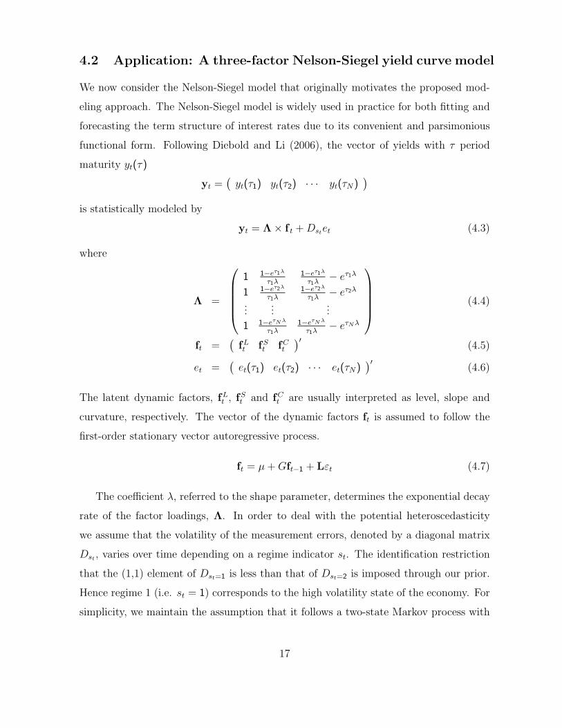
4.2 Application: A three-factor Nelson-Siegel yield curve model

We now consider the Nelson-Siegel model that originally motivates the proposed mod-

eling approach. The Nelson-Siegel model is widely used in practice for both fitting and

forecasting the term structure of interest rates due to its convenient and parsimonious

functional form. Following Diebold and Li (2006), the vector of yields with τ period

maturity yt(τ)

yt =(yt(τ1) yt(τ2) · · · yt(τN)

)is statistically modeled by

yt = Λ× f t + Dstet (4.3)

where

Λ =

1 1−eτ1λ

τ1λ1−eτ1λτ1λ− eτ1λ

1 1−eτ2λτ1λ

1−eτ2λτ1λ− eτ2λ

......

...

1 1−eτNλτ1λ

1−eτNλτ1λ

− eτNλ

(4.4)

ft =(

fLt fSt fCt)′

(4.5)

et =(et(τ1) et(τ2) · · · et(τN)

)′(4.6)

The latent dynamic factors, fLt , fSt and fCt are usually interpreted as level, slope and

curvature, respectively. The vector of the dynamic factors ft is assumed to follow the

first-order stationary vector autoregressive process.

ft = µ + Gft−1 + Lεt (4.7)

The coefficient λ, referred to the shape parameter, determines the exponential decay

rate of the factor loadings, Λ. In order to deal with the potential heteroscedasticity

we assume that the volatility of the measurement errors, denoted by a diagonal matrix

Dst , varies over time depending on a regime indicator st. The identification restriction

that the (1,1) element of Dst=1 is less than that of Dst=2 is imposed through our prior.

Hence regime 1 (i.e. st = 1) corresponds to the high volatility state of the economy. For

simplicity, we maintain the assumption that it follows a two-state Markov process with

17

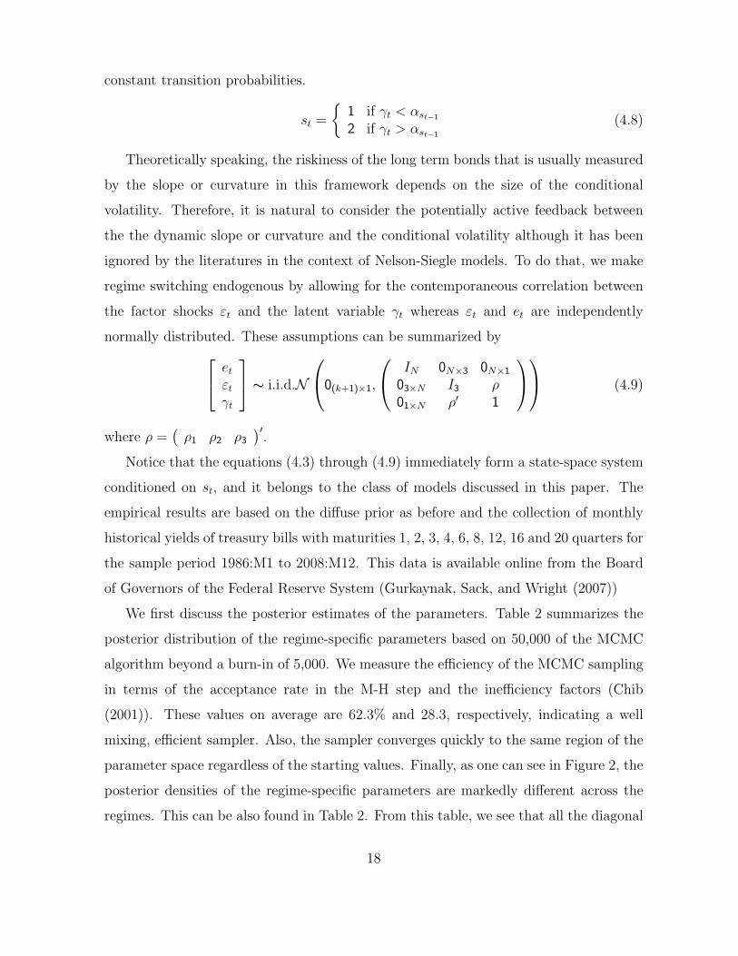
constant transition probabilities.

st =

1 if γt < αst−1

2 if γt > αst−1

(4.8)

Theoretically speaking, the riskiness of the long term bonds that is usually measured

by the slope or curvature in this framework depends on the size of the conditional

volatility. Therefore, it is natural to consider the potentially active feedback between

the the dynamic slope or curvature and the conditional volatility although it has been

ignored by the literatures in the context of Nelson-Siegle models. To do that, we make

regime switching endogenous by allowing for the contemporaneous correlation between

the factor shocks εt and the latent variable γt whereas εt and et are independently

normally distributed. These assumptions can be summarized by etεtγt

∼ i.i.d.N

0(k+1)×1,

IN 0N×3 0N×1

03×N I3 ρ01×N ρ′ 1

(4.9)

where ρ =(ρ1 ρ2 ρ3

)′.

Notice that the equations (4.3) through (4.9) immediately form a state-space system

conditioned on st, and it belongs to the class of models discussed in this paper. The

empirical results are based on the diffuse prior as before and the collection of monthly

historical yields of treasury bills with maturities 1, 2, 3, 4, 6, 8, 12, 16 and 20 quarters for

the sample period 1986:M1 to 2008:M12. This data is available online from the Board

of Governors of the Federal Reserve System (Gurkaynak, Sack, and Wright (2007))

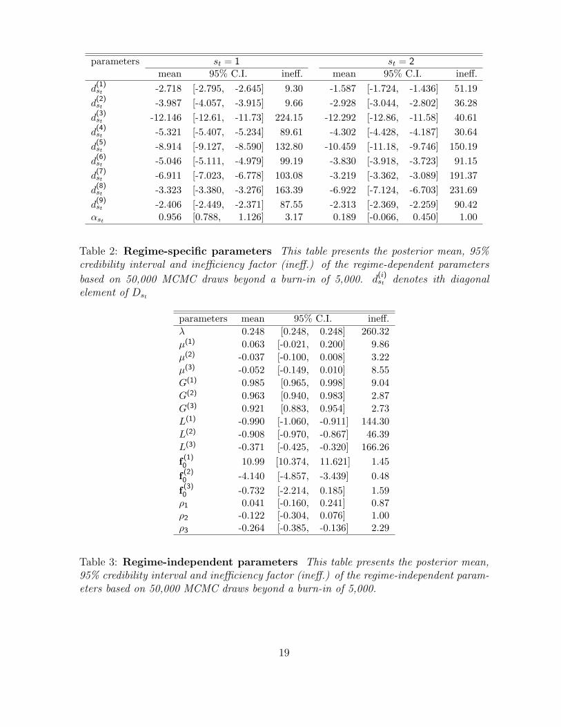
We first discuss the posterior estimates of the parameters. Table 2 summarizes the

posterior distribution of the regime-specific parameters based on 50,000 of the MCMC

algorithm beyond a burn-in of 5,000. We measure the efficiency of the MCMC sampling

in terms of the acceptance rate in the M-H step and the inefficiency factors (Chib

(2001)). These values on average are 62.3% and 28.3, respectively, indicating a well

mixing, efficient sampler. Also, the sampler converges quickly to the same region of the

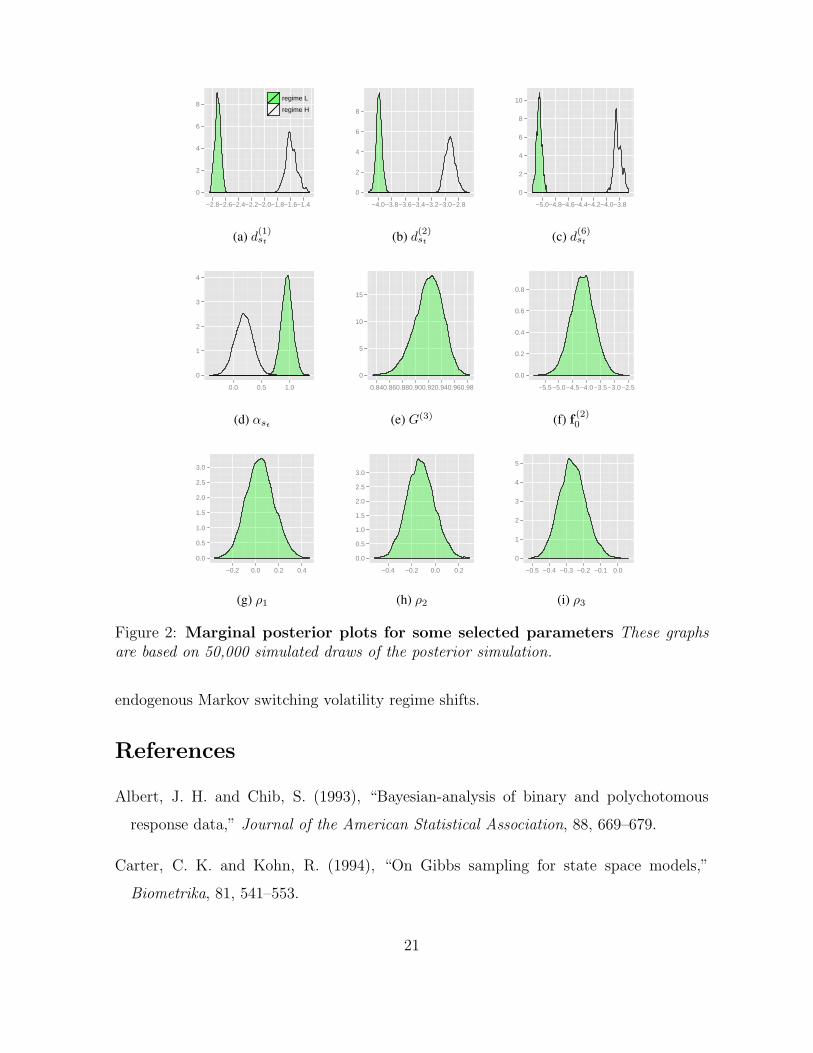
parameter space regardless of the starting values. Finally, as one can see in Figure 2, the

posterior densities of the regime-specific parameters are markedly different across the

regimes. This can be also found in Table 2. From this table, we see that all the diagonal

18

parameters st = 1 st = 2mean 95% C.I. ineff. mean 95% C.I. ineff.

d(1)st -2.718 [-2.795, -2.645] 9.30 -1.587 [-1.724, -1.436] 51.19d

(2)st -3.987 [-4.057, -3.915] 9.66 -2.928 [-3.044, -2.802] 36.28d

(3)st -12.146 [-12.61, -11.73] 224.15 -12.292 [-12.86, -11.58] 40.61d

(4)st -5.321 [-5.407, -5.234] 89.61 -4.302 [-4.428, -4.187] 30.64d

(5)st -8.914 [-9.127, -8.590] 132.80 -10.459 [-11.18, -9.746] 150.19d

(6)st -5.046 [-5.111, -4.979] 99.19 -3.830 [-3.918, -3.723] 91.15d

(7)st -6.911 [-7.023, -6.778] 103.08 -3.219 [-3.362, -3.089] 191.37d

(8)st -3.323 [-3.380, -3.276] 163.39 -6.922 [-7.124, -6.703] 231.69d

(9)st -2.406 [-2.449, -2.371] 87.55 -2.313 [-2.369, -2.259] 90.42αst 0.956 [0.788, 1.126] 3.17 0.189 [-0.066, 0.450] 1.00

Table 2: Regime-specific parameters This table presents the posterior mean, 95%credibility interval and inefficiency factor (ineff.) of the regime-dependent parameters

based on 50,000 MCMC draws beyond a burn-in of 5,000. d(i)st denotes ith diagonal

element of Dst

parameters mean 95% C.I. ineff.λ 0.248 [0.248, 0.248] 260.32µ(1) 0.063 [-0.021, 0.200] 9.86µ(2) -0.037 [-0.100, 0.008] 3.22µ(3) -0.052 [-0.149, 0.010] 8.55G(1) 0.985 [0.965, 0.998] 9.04G(2) 0.963 [0.940, 0.983] 2.87G(3) 0.921 [0.883, 0.954] 2.73L(1) -0.990 [-1.060, -0.911] 144.30L(2) -0.908 [-0.970, -0.867] 46.39L(3) -0.371 [-0.425, -0.320] 166.26f (1)0 10.99 [10.374, 11.621] 1.45f (2)0 -4.140 [-4.857, -3.439] 0.48f (3)0 -0.732 [-2.214, 0.185] 1.59ρ1 0.041 [-0.160, 0.241] 0.87ρ2 -0.122 [-0.304, 0.076] 1.00ρ3 -0.264 [-0.385, -0.136] 2.29

Table 3: Regime-independent parameters This table presents the posterior mean,95% credibility interval and inefficiency factor (ineff.) of the regime-independent param-eters based on 50,000 MCMC draws beyond a burn-in of 5,000.

19

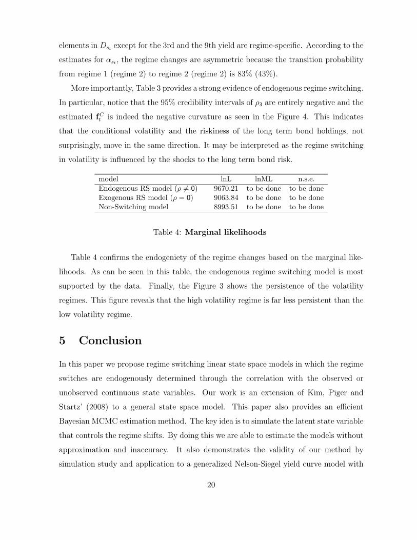
elements in Dst except for the 3rd and the 9th yield are regime-specific. According to the

estimates for αst , the regime changes are asymmetric because the transition probability

from regime 1 (regime 2) to regime 2 (regime 2) is 83% (43%).

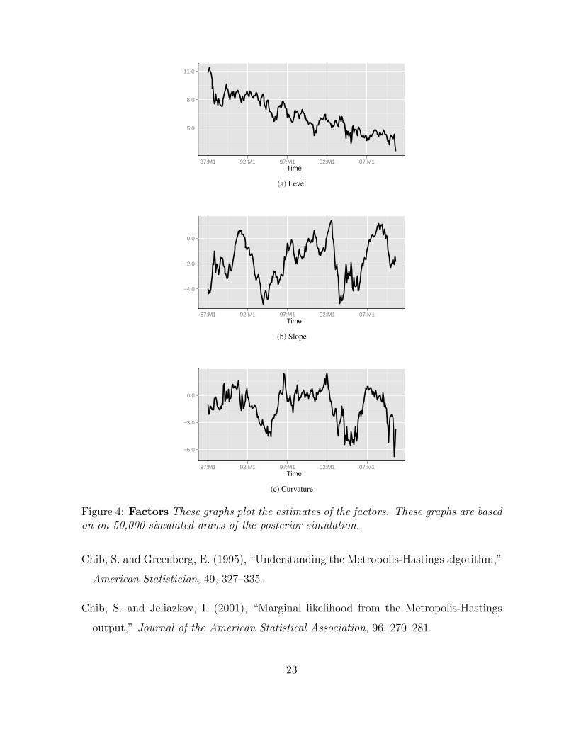
More importantly, Table 3 provides a strong evidence of endogenous regime switching.

In particular, notice that the 95% credibility intervals of ρ3 are entirely negative and the

estimated fCt is indeed the negative curvature as seen in the Figure 4. This indicates

that the conditional volatility and the riskiness of the long term bond holdings, not

surprisingly, move in the same direction. It may be interpreted as the regime switching

in volatility is influenced by the shocks to the long term bond risk.

model lnL lnML n.s.e.Endogenous RS model (ρ 6= 0) 9670.21 to be done to be doneExogenous RS model (ρ = 0) 9063.84 to be done to be doneNon-Switching model 8993.51 to be done to be done

Table 4: Marginal likelihoods

Table 4 confirms the endogeniety of the regime changes based on the marginal like-

lihoods. As can be seen in this table, the endogenous regime switching model is most

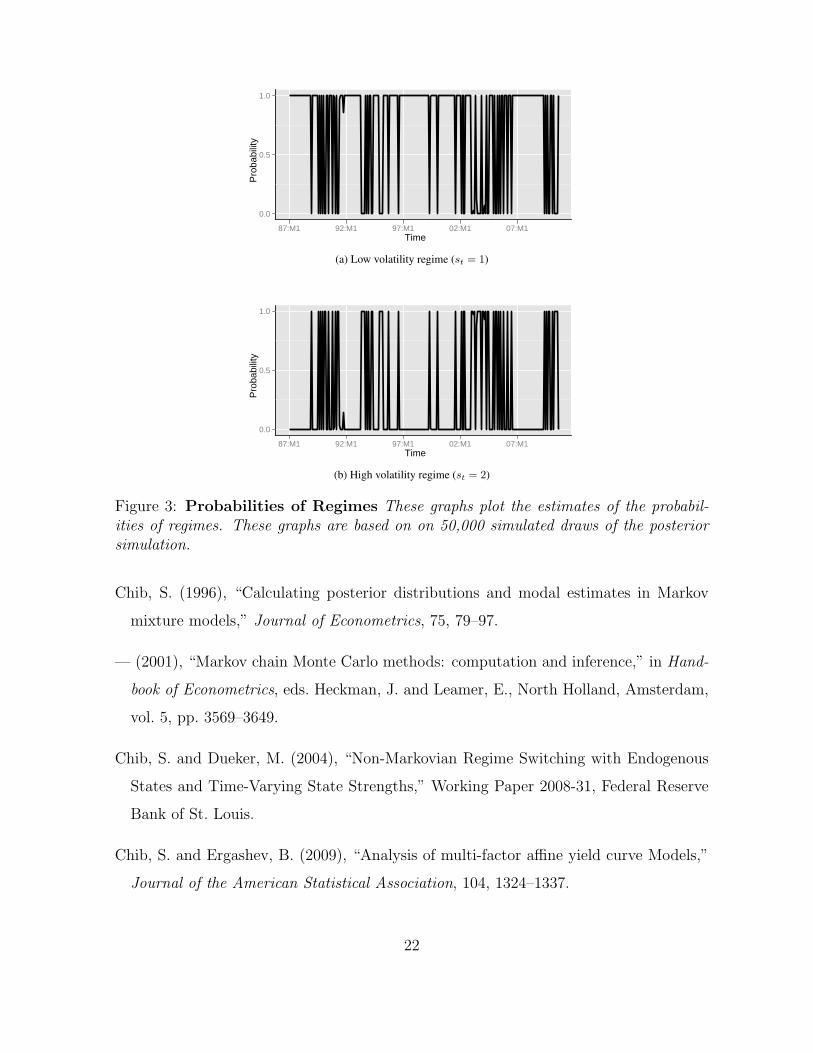
supported by the data. Finally, the Figure 3 shows the persistence of the volatility

regimes. This figure reveals that the high volatility regime is far less persistent than the

low volatility regime.

5 Conclusion

In this paper we propose regime switching linear state space models in which the regime

switches are endogenously determined through the correlation with the observed or

unobserved continuous state variables. Our work is an extension of Kim, Piger and

Startz’ (2008) to a general state space model. This paper also provides an efficient

Bayesian MCMC estimation method. The key idea is to simulate the latent state variable

that controls the regime shifts. By doing this we are able to estimate the models without

approximation and inaccuracy. It also demonstrates the validity of our method by

simulation study and application to a generalized Nelson-Siegel yield curve model with

20

0

2

4

6

8

−2.8−2.6−2.4−2.2−2.0−1.8−1.6−1.4

regime L

regime H

0

2

4

6

8

−4.0−3.8−3.6−3.4−3.2−3.0−2.8

0

2

4

6

8

10

−5.0−4.8−4.6−4.4−4.2−4.0−3.8

(a) d(1)st (b) d(2)

st (c) d(6)st

0

1

2

3

4

0.0 0.5 1.0

0

5

10

15

0.840.860.880.900.920.940.960.98

0.0

0.2

0.4

0.6

0.8

−5.5−5.0−4.5−4.0−3.5−3.0−2.5

(d) αst(e) G(3) (f) f (2)

0

0.0

0.5

1.0

1.5

2.0

2.5

3.0

−0.2 0.0 0.2 0.4

0.0

0.5

1.0

1.5

2.0

2.5

3.0

−0.4 −0.2 0.0 0.2

0

1

2

3

4

5

−0.5 −0.4 −0.3 −0.2 −0.1 0.0

(g) ρ1 (h) ρ2 (i) ρ3

Figure 2: Marginal posterior plots for some selected parameters These graphsare based on 50,000 simulated draws of the posterior simulation.

endogenous Markov switching volatility regime shifts.

References

Albert, J. H. and Chib, S. (1993), “Bayesian-analysis of binary and polychotomous

response data,” Journal of the American Statistical Association, 88, 669–679.

Carter, C. K. and Kohn, R. (1994), “On Gibbs sampling for state space models,”

Biometrika, 81, 541–553.

21

Time

Pro

babi

lity

0.0

0.5

1.0

87:M1 92:M1 97:M1 02:M1 07:M1

(a) Low volatility regime (st = 1)

Time

Pro

babi

lity

0.0

0.5

1.0

87:M1 92:M1 97:M1 02:M1 07:M1

(b) High volatility regime (st = 2)

Figure 3: Probabilities of Regimes These graphs plot the estimates of the probabil-ities of regimes. These graphs are based on on 50,000 simulated draws of the posteriorsimulation.

Chib, S. (1996), “Calculating posterior distributions and modal estimates in Markov

mixture models,” Journal of Econometrics, 75, 79–97.

— (2001), “Markov chain Monte Carlo methods: computation and inference,” in Hand-

book of Econometrics, eds. Heckman, J. and Leamer, E., North Holland, Amsterdam,

vol. 5, pp. 3569–3649.

Chib, S. and Dueker, M. (2004), “Non-Markovian Regime Switching with Endogenous

States and Time-Varying State Strengths,” Working Paper 2008-31, Federal Reserve

Bank of St. Louis.

Chib, S. and Ergashev, B. (2009), “Analysis of multi-factor affine yield curve Models,”

Journal of the American Statistical Association, 104, 1324–1337.

22

Time

5.0

8.0

11.0

87:M1 92:M1 97:M1 02:M1 07:M1

(a) Level

Time

−4.0

−2.0

0.0

87:M1 92:M1 97:M1 02:M1 07:M1

(b) Slope

Time

−6.0

−3.0

0.0

87:M1 92:M1 97:M1 02:M1 07:M1

(c) Curvature

Figure 4: Factors These graphs plot the estimates of the factors. These graphs are basedon on 50,000 simulated draws of the posterior simulation.

Chib, S. and Greenberg, E. (1995), “Understanding the Metropolis-Hastings algorithm,”

American Statistician, 49, 327–335.

Chib, S. and Jeliazkov, I. (2001), “Marginal likelihood from the Metropolis-Hastings

output,” Journal of the American Statistical Association, 96, 270–281.

23

Chib, S. and Ramamurthy, S. (2010), “Tailored Randomized-block MCMC Methods

with Application to DSGE Models,” Journal of Econometrics, 155, 19–38.

Cochrane, J. H. and Piazzesi, M. (2008), “Decomposing the Yield Curve,” Manuscript.

Diebold, F. X. and Li, C. L. (2006), “Forecasting the term structure of government bond

yields,” Journal of Econometrics, 130, 337–364.

Gurkaynak, R. S., Sack, B., and Wright, J. H. (2007), “The U.S. treasury yield curve:

1961 to the present,” Journal of Monetary Economics, 54, 2291–2304.

Hamilton, J. (1989), “A new approach to the economic analysis of nonstationary time

series and the business cycle,” Econometrica, 57, 357–84.

Kim, C. J. (1994), “Dynamic linear models with Markov-switching,” Journal of Econo-

metrics, 60, 1–22.

Kim, C. J. and Nelson, C. R. (1998), “Business Cycle Turning Points, A New Coincident

Index, and Tests of Duration Dependence Based on a Dynamic Factor Model With

Regime Switching,” Review of Economics and Statistics, 80, 188–201.

Kim, C. J. and Piger, J. (2002), “Dynamic linear models with Markov-switching,” Jour-

nal of Monetary Economics, 49, 1189–1211.

Kim, C. J., Piger, J., and Startz, R. (2008), “Estimation of Markov regime-switching

regression models with endogenous switching,” Journal of Econometrics, 143, 263–

273.

Kuan, C.-M., Huang, Y.-L., and Tsay, R. S. (2005), “An Unobserved-Component Model

With Switching Permanent and Transitory Innovations,” Journal of Business and

Economic Statistics, 23, 443–454.

Morley, J., Nelson, C. R., and Zivot, E. (2003), “Why Are Unobserved Component

and Beveridge-Nelson Trend-Cycle Decompositions of GDP So Different,” Review of

Economics and Statistics, 85, 235–243.

24

Sinclair, T. M. (2010), “Asymmetry in the Business Cycle: Friedman’s Plucking Model

with Correlated Innovations,” Studies in Nonlinear Dynamics and Econometrics, 14,

235–243.

25