State-Space Design Method for ControlSystems

OverviewThis tutorial shows how to use the state-space design method for control systems, using LabVIEW 8.2 with theLabVIEW Control Design Toolkit.

These tutorials are based on the Control Tutorials developed by Professor Dawn Tilbury of the Mechanical Engineeringdepartment at the University of Michigan and Professor Bill Messner of the Department of Mechanical Engineering atCarnegie Mellon University and were developed with their permission.

Frequency Response Controls Tutorials Menu Digital Control

State-Space Equations

There are several different ways to describe a system of linear differential equations. The state-space representation isgiven by the following equations:

In these equations, x is an n-by-1 vector representing the state (commonly position and velocity variable in mechanicalsystems), u is a scalar representing the input (commonly a force or torque in mechanical systems), and y is a scalarrepresenting the output. The matrices A (n by n), B (n by 1), and C (1 by n) determine the relationships between thestate and input and output variable. Note that there are n first-order differential equations. State space representation canalso be used for systems with multiple inputs and outputs (MIMO), but we will only use single-input, single-output(SISO) systems in these tutorials.

To introduce the state space design method, we will use the magnetically suspended ball as an example. The currentthrough the coils induces a magnetic force which can balance the force of gravity and cause the ball (which is made of amagnetic material) to be suspended in midair. The modeling of this system has been established in many control textbooks (including Automatic Control Systems by B. C. Kuo, seventh edition).

LabVIEW™, National Instruments™, and ni.com™ are trademarks of National Instruments Corporation. Product and company names mentioned herein are trademarks or trade names of theirrespective companies. For patents covering National Instruments products, refer to the appropriate location: Help»patents in your software, the patents.txt file on your CD, or ni.com/patents.

© Copyright 2006 National Instruments Corporation. All rights reserved. Document Version 31

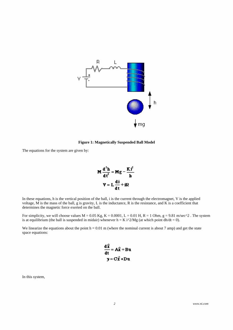
Figure 1: Magnetically Suspended Ball Model

The equations for the system are given by:

In these equations, h is the vertical position of the ball, i is the current through the electromagnet, V is the appliedvoltage, M is the mass of the ball, g is gravity, L is the inductance, R is the resistance, and K is a coefficient thatdetermines the magnetic force exerted on the ball.

For simplicity, we will choose values M = 0.05 Kg, K = 0.0001, L = 0.01 H, R = 1 Ohm, g = 9.81 m/sec^2 . The systemis at equilibrium (the ball is suspended in midair) whenever h = K i^2/Mg (at which point dh/dt = 0).

We linearize the equations about the point h = 0.01 m (where the nominal current is about 7 amp) and get the statespace equations:

In this system,

2 www.ni.com

is the set of state variables for the system (a 3x1 vector), u is the input voltage (delta V), and y (the output), is delta h.

Hybrid Graphical/MathScript Approach

To use this system in LabVIEW, create a new VI and insert a MathScript Node (from the Structures palette).

Enter the system matrices using the following code:

A = [ 0 1 0

980 0 -2.8

0 0 -100];

B = [0

0

100];

C = [1 0 0];

LabVIEW MathScript Approach

Alternatively, you can open the MathScript Window (Tools » MathScript Window).

Enter the system matrices using the following code:

A = [ 0 1 0

980 0 -2.8

0 0 -100];

B = [0

0

100];

C = [1 0 0];

Finding the Poles of the System

One of the first things you want to do with the state equations is find the poles of the system. These are the values of swhere det(sI - A) = 0, or the eigenvalues of the A matrix.

Hybrid Graphical/MathScript Approach

To do this using the hybrid graphical/MathScript programming approach, add the CD Pole-Zero Map VI to your block

3 www.ni.com

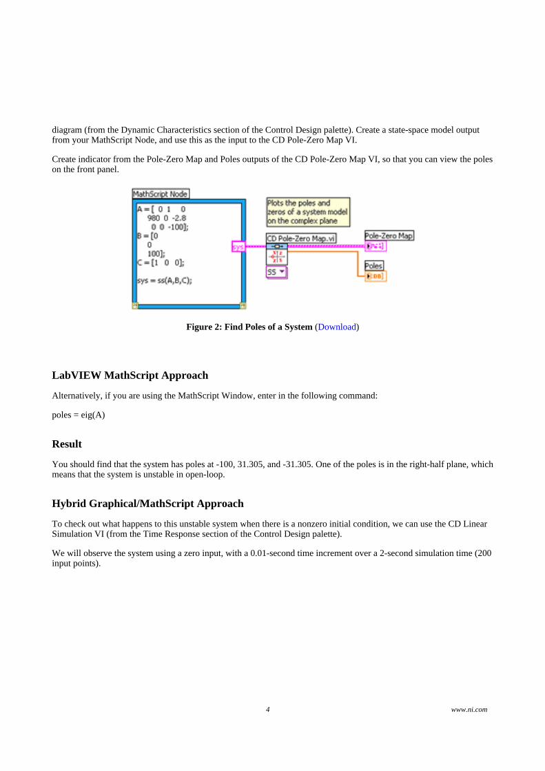
diagram (from the Dynamic Characteristics section of the Control Design palette). Create a state-space model outputfrom your MathScript Node, and use this as the input to the CD Pole-Zero Map VI.

Create indicator from the Pole-Zero Map and Poles outputs of the CD Pole-Zero Map VI, so that you can view the poleson the front panel.

Figure 2: Find Poles of a System (Download)

LabVIEW MathScript Approach

Alternatively, if you are using the MathScript Window, enter in the following command:

poles = eig(A)

Result

You should find that the system has poles at -100, 31.305, and -31.305. One of the poles is in the right-half plane, whichmeans that the system is unstable in open-loop.

Hybrid Graphical/MathScript Approach

To check out what happens to this unstable system when there is a nonzero initial condition, we can use the CD LinearSimulation VI (from the Time Response section of the Control Design palette).

We will observe the system using a zero input, with a 0.01-second time increment over a 2-second simulation time (200input points).

4 www.ni.com

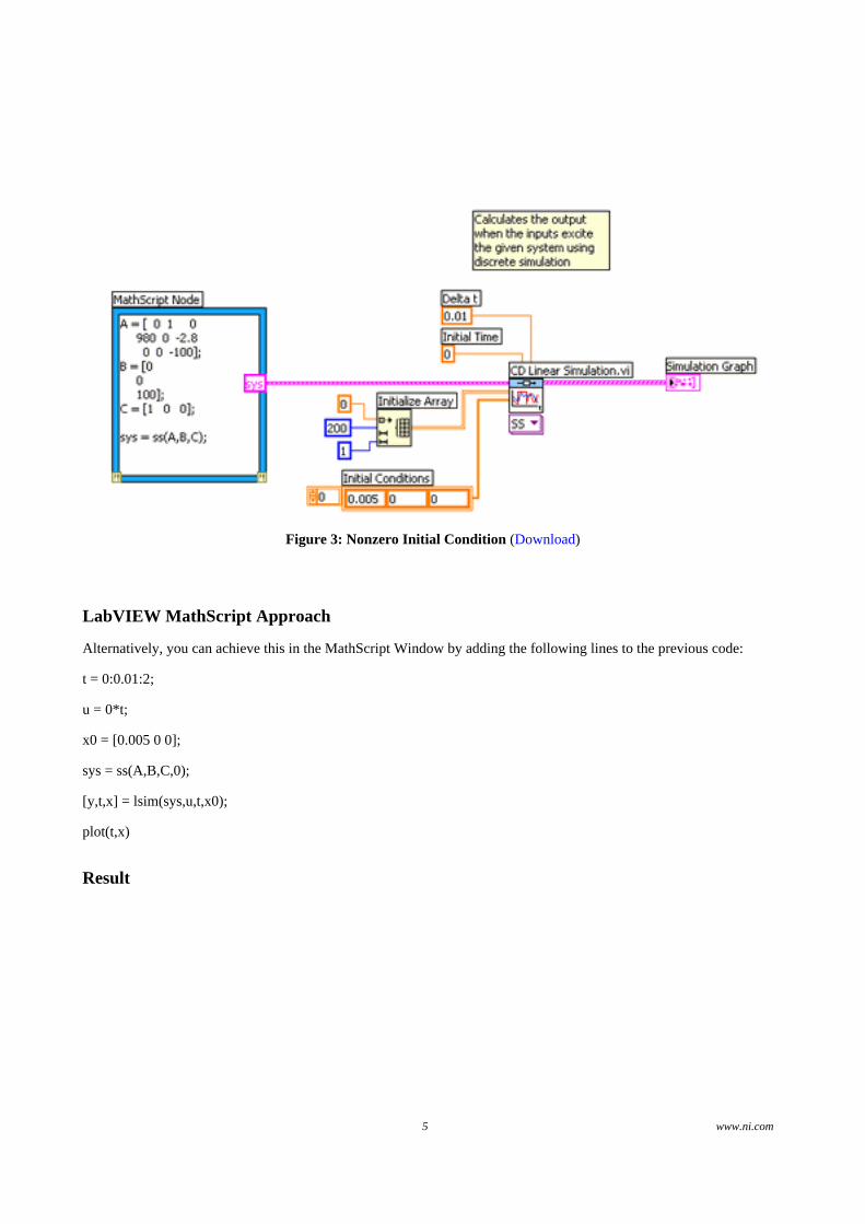
Figure 3: Nonzero Initial Condition (Download)

LabVIEW MathScript Approach

Alternatively, you can achieve this in the MathScript Window by adding the following lines to the previous code:

t = 0:0.01:2;

u = 0*t;

x0 = [0.005 0 0];

sys = ss(A,B,C,0);

[y,t,x] = lsim(sys,u,t,x0);

plot(t,x)

Result

5 www.ni.com

Figure 4: Open-Loop Response to Nonzero Initial Condition

The green line on the graph in Figure 4 shows us that the distance between the ball and the electromagnet will go toinfinity, but the ball probably hits the table or the floor first (and also probably goes out of the range where ourlinearization is valid).

Control Design Using Pole Placement

Let's build a controller for this system. The schematic of a full-state feedback system is the following:

Figure 5: Full-State Feedback System

Recall that the characteristic polynomial for this closed-loop system is the determinant of (sI-(A-BK)). Since thematrices A and B*K are both 3 by 3 matrices, there will be 3 poles for the system. By using full-state feedback we can

6 www.ni.com

place the poles anywhere we want. We could use the MathScript functionackerto find the control matrix, K, which will give the desired poles.

Before attempting this method, we have to decide where we want the closed-loop poles to be. Suppose the criteria forthe controller were settling time < 0.5 sec and overshoot < 5%. We might then try to place the two dominantpoles at -10 +/- 10i (at zeta = 0.7 or 45 degrees with sigma = 10 > 4.6*2). We might place the third pole at -50 tostart, and we can change it later depending on what the closed-loop behavior is.

Hybrid Graphical/MathScript Approach

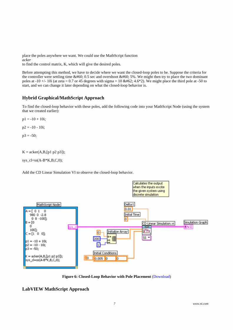
To find the closed-loop behavior with these poles, add the following code into your MathScript Node (using the systemthat we created earlier):

p1 = -10 + 10i;

p2 = -10 - 10i;

p3 = -50;

K = acker(A,B,[p1 p2 p3]);

sys_cl=ss(A-B*K,B,C,0);

Add the CD Linear Simulation VI to observe the closed-loop behavior.

Figure 6: Closed-Loop Behavior with Pole Placement (Download)

LabVIEW MathScript Approach

7 www.ni.com

Alternatively, input the following code if you are using the MathScript Window:

p1 = -10 + 10i;

p2 = -10 - 10i;

p3 = -50;

K = acker(A,B,[p1 p2 p3]);

sys_cl=ss(A-B*K,B,C,0);

[y,t,x] = lsim(sys_cl,u,t,x0);

plot(t,y)

Result

Figure 7: Ball Position (m) Versus Time (s)

Observe that the overshoot is too large (there are also zeros in the transfer function which can increase the overshoot;you do not see the zeros in the state-space formulation).

Try placing the poles further to the left to see if the transient response improves (this should also make the responsefaster).

8 www.ni.com

Hybrid Graphical/MathScript Approach

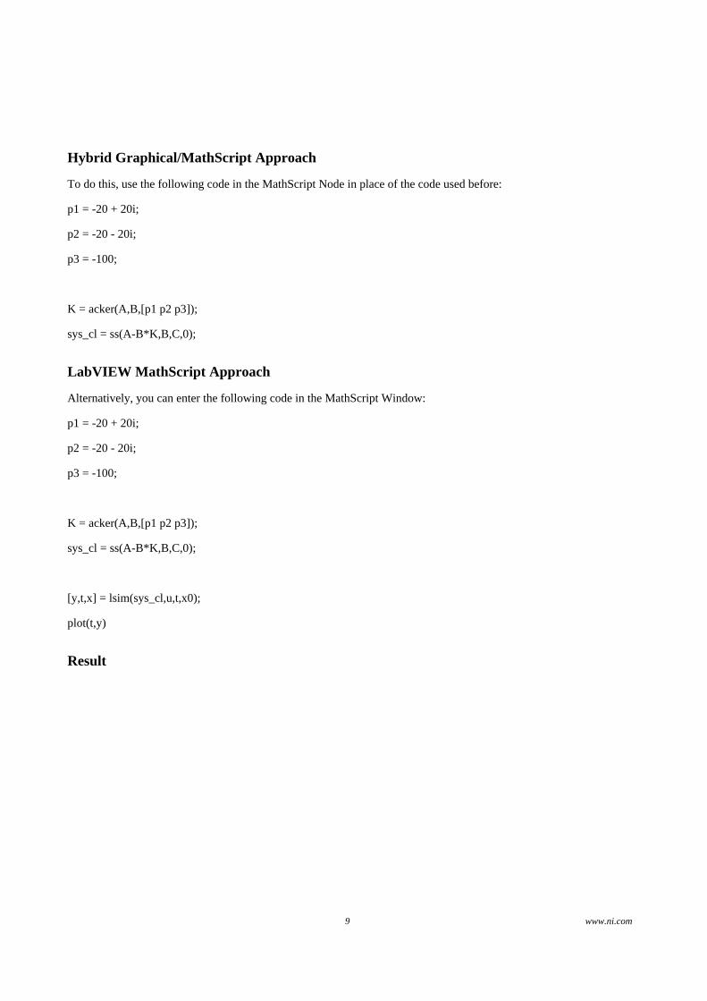
To do this, use the following code in the MathScript Node in place of the code used before:

p1 = -20 + 20i;

p2 = -20 - 20i;

p3 = -100;

K = acker(A,B,[p1 p2 p3]);

sys_cl = ss(A-B*K,B,C,0);

LabVIEW MathScript Approach

Alternatively, you can enter the following code in the MathScript Window:

p1 = -20 + 20i;

p2 = -20 - 20i;

p3 = -100;

K = acker(A,B,[p1 p2 p3]);

sys_cl = ss(A-B*K,B,C,0);

[y,t,x] = lsim(sys_cl,u,t,x0);

plot(t,y)

Result

9 www.ni.com

Figure 8: Ball Position (m) Versus Time (s) – New Pole Placement

This time the overshoot is smaller. Compare the control effort required (K) in both cases. In general, the farther youmove the poles, the more control effort it takes.

Introducing the Reference Input

Now we will take the control system as defined above and apply a step input (we choose a small value for the step, sowe remain in the region where our linearization is valid).

Hybrid Graphical/MathScript Approach

Remove the initial conditions, and change the input signal to have a constant value of 0.001.

10 www.ni.com

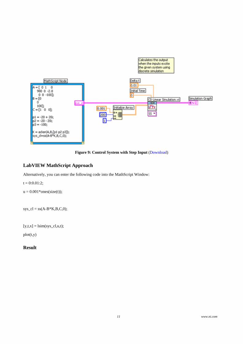
Figure 9: Control System with Step Input (Download)

LabVIEW MathScript Approach

Alternatively, you can enter the following code into the MathScript Window:

t = 0:0.01:2;

u = 0.001*ones(size(t));

sys_cl = ss(A-B*K,B,C,0);

[y,t,x] = lsim(sys_cl,u,t);

plot(t,y)

Result

11 www.ni.com

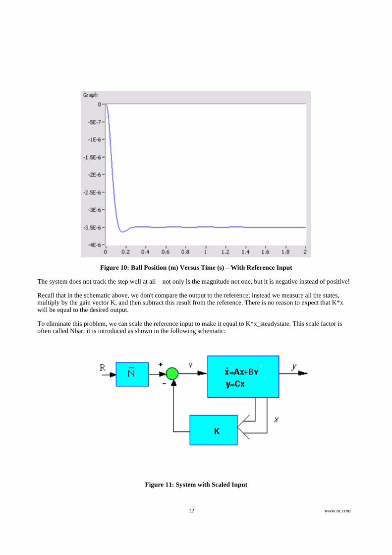
Figure 10: Ball Position (m) Versus Time (s) – With Reference Input

The system does not track the step well at all – not only is the magnitude not one, but it is negative instead of positive!

Recall that in the schematic above, we don't compare the output to the reference; instead we measure all the states,multiply by the gain vector K, and then subtract this result from the reference. There is no reason to expect that K*xwill be equal to the desired output.

To eliminate this problem, we can scale the reference input to make it equal to K*x_steadystate. This scale factor isoften called Nbar; it is introduced as shown in the following schematic:

Figure 11: System with Scaled Input

12 www.ni.com

We can calculate Nbar by using the custom function r_scale. Note that this function is not native to LabVIEWMathScript. You will need to download the m-file to use it.

Download this file and save it to your LabVIEW Data folder (usually located in My Documents » LabVIEW Data).

Next, open the MathScript Window (Tools » MathScript Window). Select File » Load Script, and select the filer_scale.m.

Finally, select File » Save and Compile Script. Now you can use this custom function as a command in MathScript.

Since we want to find the response of the system under state feedback with this introduction of the reference, we simplynote the fact that the input is multiplied by this new factor, Nbar.

Hybrid Graphical/MathScript Approach

Using the VI from Figure 9, add the following line of code:

Nbar=r_scale(sys_cl,K);

Create an output from the MathScript Node for Nbar, and scale the input signal by this factor.

Figure 12: Block Diagram for System with Scaled Reference Input (Download)

LabVIEW MathScript Approach

Alternatively, you can achieve this by using the MathScript Window. Add the following code to what you previouslyentered:

Nbar=r_scale(sys_cl,K)

13 www.ni.com

[y,t,x] = lsim(sys_cl,Nbar*u,t);

plot(t,y)

Result

Figure 13: System Response with Nbar

A step can now be tracked reasonably well.

Observer Design

When we can't measure all the states x (as is commonly the case), we can build an observer to estimate them, whilemeasuring only the output y = C x. For the magnetic ball example, we will add three new, estimated states to thesystem. The schematic is as follows:

14 www.ni.com

Figure 14: System with Observer

The observer is basically a copy of the plant; it has the same input and almost the same differential equation. An extraterm compares the actual measured output y to the estimated output #; this will cause the estimated states

to approach the values of the actual states x.

The error dynamics of the observer are given by the poles of (A-L*C).

First, we need to choose the observer gain L. Since we want the dynamics of the observer to be much faster than thesystem itself, we need to place the poles at least five times farther to the left than the dominant poles of the system. Wewill place the observer poles at -100.

LabVIEW MathScript OR Hybrid Graphical/MathScript Approach

Add the following lines to your MathScript code:

op1 = -100;

op2 = -100;

op3 = -100;

Because of the duality between controllability and observability, we can use the same technique used to find the controlmatrix, but replacing the matrix B by the matrix C and taking the transposes of each matrix.

L = acker(A',C',[op1 op2 op3])';

The equations in the block diagram above are given for

. It is conventional to write the combined equations for the system plus observer using the original state x plus the errorstate: e = x -

. We use as state feedback u = -K

15 www.ni.com

.

After a little bit of algebra (consult a textbook for more details), we can arrive at the combined state and error equationswith the full-state feedback and an observer.

At = [A - B*K B*K

zeros(size(A)) A - L*C];

Bt = [B*Nbar

zeros(size(B))];

Ct = [C zeros(size(C))];

We typically assume that the observer begins with zero initial condition,

= 0. This gives us that the initial condition for the error is equal to the initial condition of the state.

Hybrid Graphical/MathScript Approach

To see how the response looks to a nonzero initial condition with no reference input, input the following line into theMathScript Node:

sys=ss(At,Bt,Ct,0);

In addition, create a constant for the Initial Conditions terminal. Set the value of this constant to [0.005 0 0].

16 www.ni.com

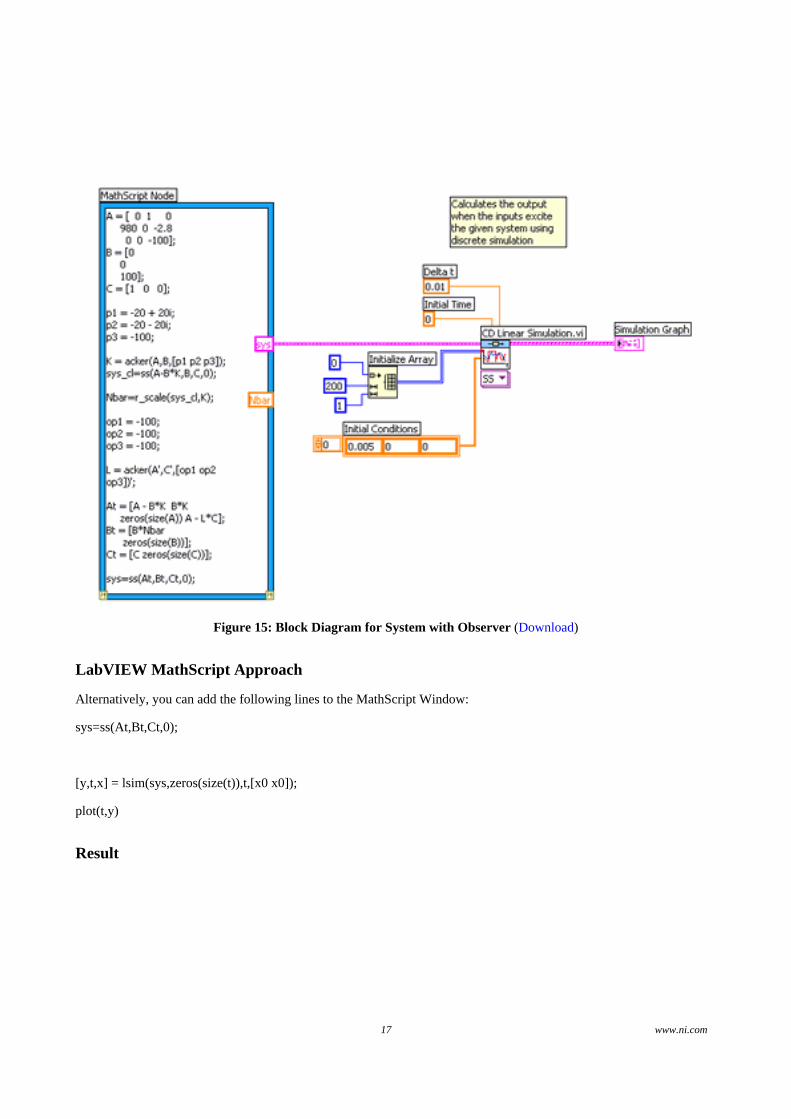
Figure 15: Block Diagram for System with Observer (Download)

LabVIEW MathScript Approach

Alternatively, you can add the following lines to the MathScript Window:

sys=ss(At,Bt,Ct,0);

[y,t,x] = lsim(sys,zeros(size(t)),t,[x0 x0]);

plot(t,y)

Result

17 www.ni.com

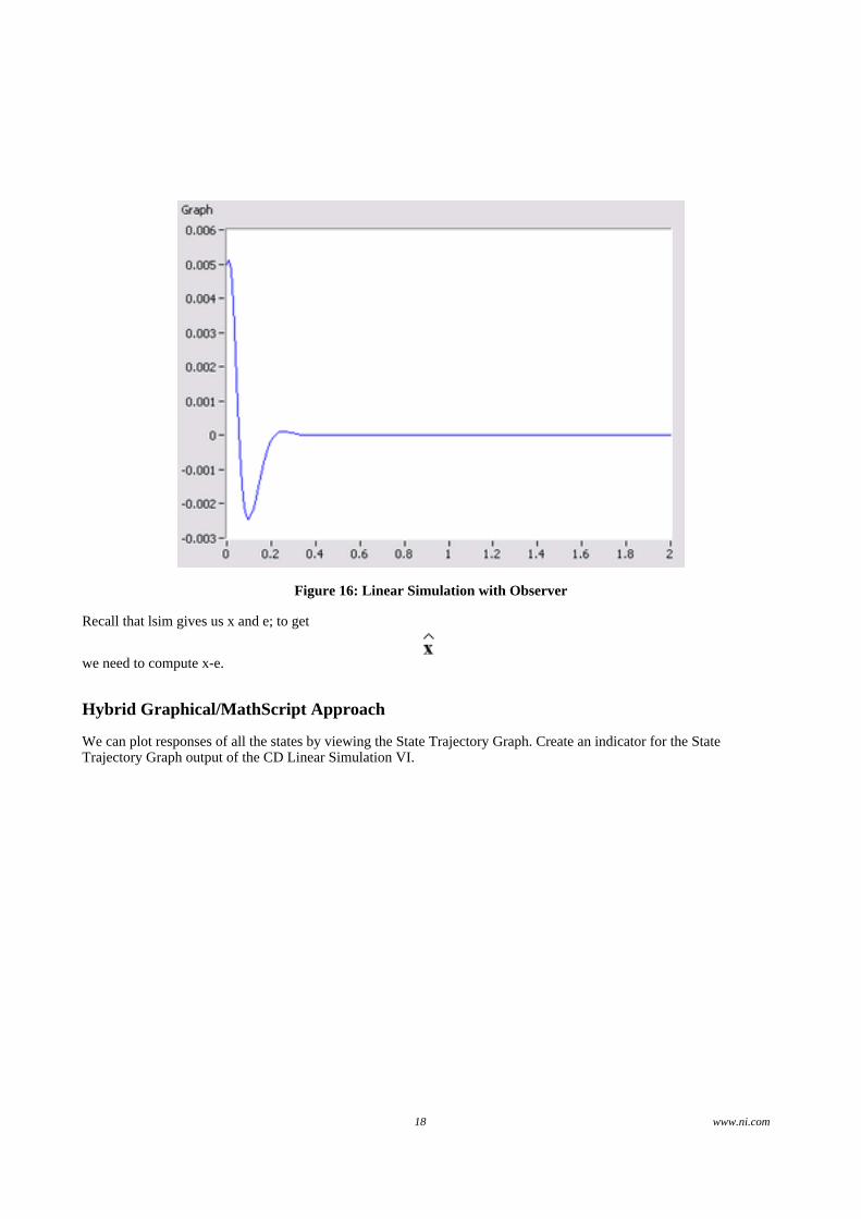
Figure 16: Linear Simulation with Observer

Recall that lsim gives us x and e; to get

we need to compute x-e.

Hybrid Graphical/MathScript Approach

We can plot responses of all the states by viewing the State Trajectory Graph. Create an indicator for the StateTrajectory Graph output of the CD Linear Simulation VI.

18 www.ni.com

Figure 17: Block Diagram for State Trajectory Graph (Download)

LabVIEW MathScript Approach

Alternatively, you can use the plot command in the MathScript Window to graph t versus x:

plot(t,x)

axis([0,.3,-2,5])

Result

You should see the plot that looks like the one shown below, in Figure 18.

19 www.ni.com

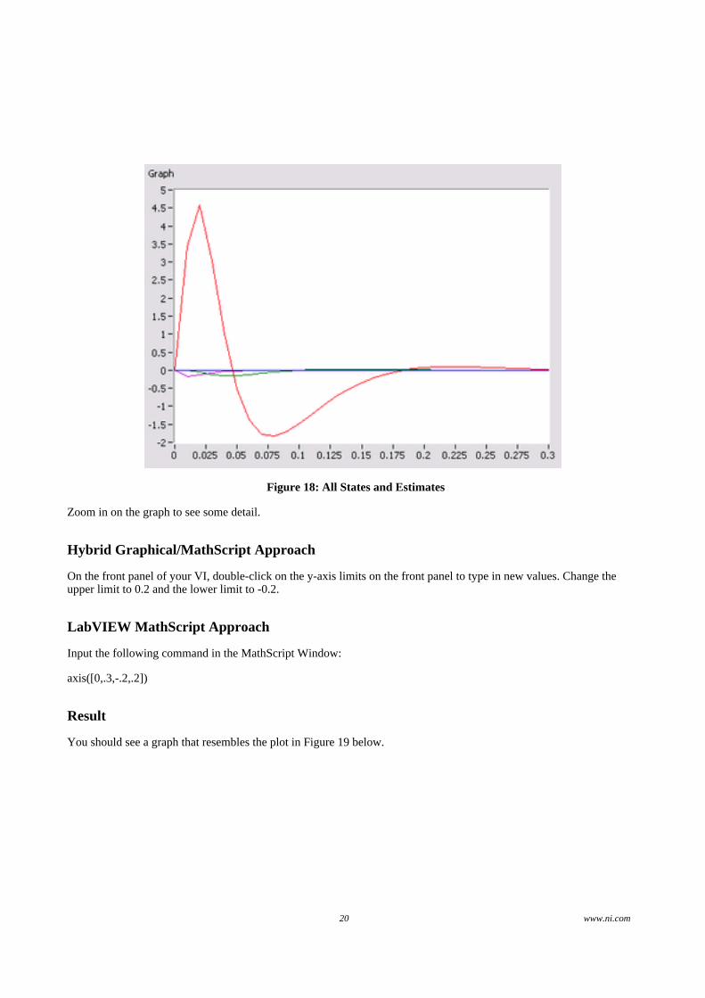
Figure 18: All States and Estimates

Zoom in on the graph to see some detail.

Hybrid Graphical/MathScript Approach

On the front panel of your VI, double-click on the y-axis limits on the front panel to type in new values. Change theupper limit to 0.2 and the lower limit to -0.2.

LabVIEW MathScript Approach

Input the following command in the MathScript Window:

axis([0,.3,-.2,.2])

Result

You should see a graph that resembles the plot in Figure 19 below.

20 www.ni.com

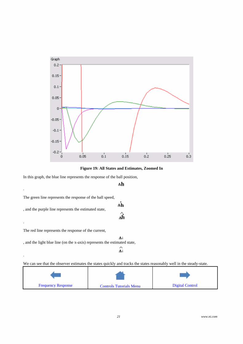
Figure 19: All States and Estimates, Zoomed In

In this graph, the blue line represents the response of the ball position,

.

The green line represents the response of the ball speed,

, and the purple line represents the estimated state,

.

The red line represents the response of the current,

, and the light blue line (on the x-axis) represents the estimated state,

.

We can see that the observer estimates the states quickly and tracks the states reasonably well in the steady-state.

Frequency Response Controls Tutorials Menu Digital Control

21 www.ni.com