State Income Inequality and Presidential Election Turnout and Outcomes

By

James K. Galbraith and Travis Hale

Galbraith@mail.utexas.edu jthale@mail.utexas.edu

The University of Texas Inequality Project Lyndon B. Johnson School of Public Affairs

The University of Texas at Austin Austin, Texas 78713

UTIP Working Paper 33

REVISED March 3, 2006

Abstract: In this paper we use a previously neglected, high-quality data source to generate consistent annual measures of income inequality by state, for the fifty United States and the District of Columbia from 1969 to 2004. We use the estimates in a model of presidential election turnout and outcomes at the state level from 1992 to 2004. In recent elections, we find that high state inequality is negatively correlated with turnout and a positively correlated with the Democratic vote share, after controlling for race and other factors.

1

Introduction The purposes of this paper are to outline a technique for estimating Gini coefficients of family income inequality for the fifty United States and the District of Columbia on an annual basis from 1969 to 2004, and to use the estimates in a model of presidential election turnout and outcomes at the state level from 1992 to 2004. Our key findings are that high inequality is associated with lower voter turnout, and, in recent years, that rising inequality tends to raise the Democratic Party’s vote share. These relationships hold after controlling for state characteristics such as race and income. From the late 1960’s through the turn of the century, the United States endured rising income inequality, as did many other developed nations. Comparative research tends to focus on the countries as a whole, but scattered evidence indicates that sub-national units vary in their inequality patterns. Using states or regions gives us more degrees of freedom for analyses of the causes and consequences of inequality, and the capacity to related inequality to political events.1 In building a continuous panel dataset of state-by-state Gini coefficients and demonstrating an application, we hope to encourage further research on American inequality at the state or regional level.2 Estimating State Gini Coefficients of Family Income This is not the first attempt to construct inequality estimates for American states.3 However, we mine a previously neglected, high-quality data source for instruments that can be used to improve estimates from previous work, and we provide consistent coverage for a longer period than other studies have done. In this section, we describe our procedure for estimating state Gini coefficients of family income, point out some interesting features, and evaluate the quality of the results.4 Assumptions and Intuition At 10-year intervals, the Census Bureau (2005a) produces two types of income inequality measures at the state level. Using data from the one-percent and five-percent long-form samples, the Census Bureau calculates family income inequality in 1969, 1979, 1989, and 1999; household estimates are also provided for the latter three years. To move from decennial to annual data, we must derive values for the interim years. Simple interpolation is possible, but it adds no new information. The alternative is to find an annual dataset that measures wages or incomes for a large proportion of the population of each state, create a panel of inequality measures using this underlying data, and then use the decennial Census values to transform these yearly inequality measures into estimates of the appropriate Gini coefficient. We pursue the second approach. Procedure The ideal dataset for constructing state inequality measures would contain individual-level income data for every American–by state–in every year. Such data do not exist. The Census Bureau’s Current Population Survey (CPS) provides the best individual-level

2

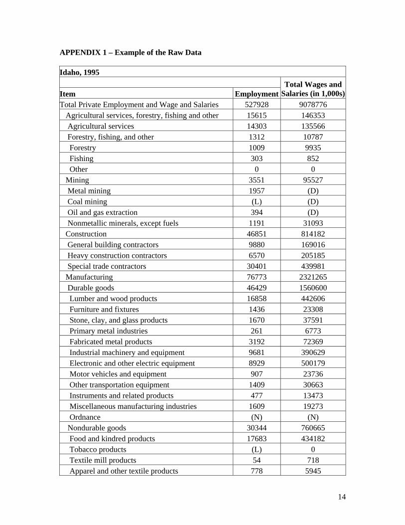
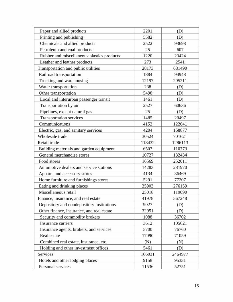
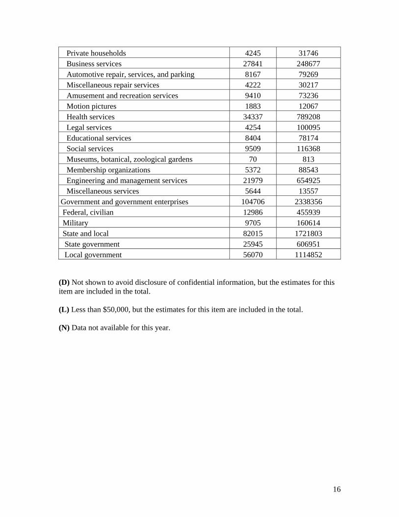
sample data available on a yearly basis. Langer (1999) estimates state Gini coefficients of household income annually from 1976 to 1995 using the CPS data. While her results surpass previous attempts to estimate state income inequality, any measure based on CPS statistics is subject to small sample sizes, a need to interpolate values within income ranges, and top-codes that truncate large reported incomes. Given the limitations of the CPS data, we consider that a group-based dataset with broad coverage that is consistent across time and space may be superior to sampled individual-level data. The Bureau of Economic Analysis (BEA) in the U.S. Department of Commerce collects data necessary to create internally consistent measures of state pay inequality for the last three decades. For every year since 1969, the BEA has compiled data on wages and employment across dozens of industrial classifications for every state. From 1969 to 2000, the data were organized along the Standard Industrial Classifications (SIC) Index; in 2001, the BEA started using the North American Industry Classification System (NAICS). Under each taxonomy, the BEA reports employment and pay totals for each sector derived directly from states’ unemployment insurance programs, IRS records, and other official sources. The main source for underlying data is the Covered Employees and Wages Program (ES-202) in the Bureau of Labor Statistics (BLS).5 Appendix 1 provides an example of the BEA data.6 Data for every state and the District of Columbia are available in this form from 1969 to 2000. For the years 2001 to 2004, the records are similar, adhering to the new classification standard. Given this data, Theil’s T statistic is an appropriate tool to evaluate pay inequality, estimating a “between-group” measure that yields a lower bound for population-wide inequality.7 While the value of the between-group inequality may be much smaller than the population-wide value, if the group structure is consistent and meaningful, the two data series tend to move together over time. (Conceição, Galbraith and Bradford, 2000.) With the inter-industrial data available, we compute between-industry pay inequality using Theil’s T statistic for every state and the nation as a whole from 1969 to 2004.8 Trends in both the state and national series of pay inequality correlate highly to the decennial income inequality measures for states. 9 Since wages and salaries compose the largest portion of income, we expect Theil’s T statistic measured on pay inequality at the state level to move closely with the census-based Gini coefficients of income inequality. Confirming our expectation, the average cross-sectional correlation between the within-state inter-sectoral Theil statistics and the Census Bureau Gini coefficients of family income in 1969, 1979, 1989, and 1999 is .710. While differences in pay inequality within states account for much of the differences in state inequality of family income, the evolution of nationwide pay inequality also closely corresponds to the income-based measures at the state level. The nationwide secular trend is so great that the average correlation between the national-level inter-industrial Theil statistic of pay inequality and the census-based Gini coefficients of family income at the state level for the overlapping years is .936, stronger than the correlation of the two within-state measures.

3

The close connection of the national values and the individual state series has two related explanations. First, because the national economy is highly integrated, many of the same factors that contribute to inter-industrial pay inequality at the national level will filter down to the states. For example, if durable manufacturing industries make gains vis-à-vis the service sectors at the national level, then the same trend will occur in many states. Second, national-level inter-industrial pay inequality picks up broad macroeconomic factors that will affect sources of non-wage income. Interest and dividend incomes, rents, capital gains, and transfer payments are related to regional and national political, social, and economic forces and these will be better captured by a national than by a specific state’s inequality measure. For example, whereas the information-technology bubble led to sharp rises in pay inequality in California, Washington, and other states, the dot com boom could also have increased income inequality in states without much high technology industry via ownership patterns in the capital markets. To maintain the heterogeneity of the within-state variation yet also incorporate the common national factors, we create a synthetic measure of within-state income inequality that incorporates influences from both state and national pay inequality measures. For each state, we add the inter-industrial Theil statistic of pay within the state to the inter-industrial Theil statistic of pay at the national level, multiplied by a state-specific weighting factor that makes the average of the two Theil statistics equal in magnitude over the 35 years for each state. We find that, on average, these linear combinations of the state and national inter-industrial pay inequality measures correlate better to states’ Census Gini coefficients than either the state or the national series alone. The average correlation between the additive measure of state and national Theil statistics of pay inequality and the state census-based Gini coefficients of family income for the overlapping years is .946. Now armed with a panel series of inequality measures based on inter-industrial Theil statistics of pay, we use ordinary least squares regression models to relate these values to the Census Gini coefficient values for the overlapping years – 1969, 1979, 1989, 1999.10 Once we have the regression coefficients (with separate estimates for each state), we can interpolate the years between censuses.11 Evaluating the Estimates We first show an application of an inter-industrial Theil statistic that closely corresponds with the Gini coefficient of the same population. Values of Theil’s T statistic for pay inequality at the national level using employment and wage data for approximately 80 sectors over the years 1969 – 2000 and annual Gini coefficient estimates of national household income inequality as measured by the CPS have a correlation coefficient of .947. 12 As discussed above, the Theil-based values of pay inequality and decennial Gini coefficients of income inequality have an average time-series correlation of .946 across the states. Furthermore, 43 states register a correlation of greater than .90, and none is

4

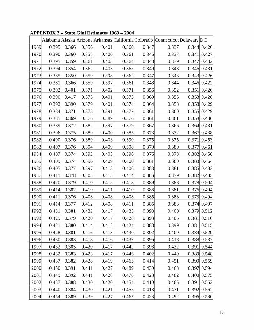
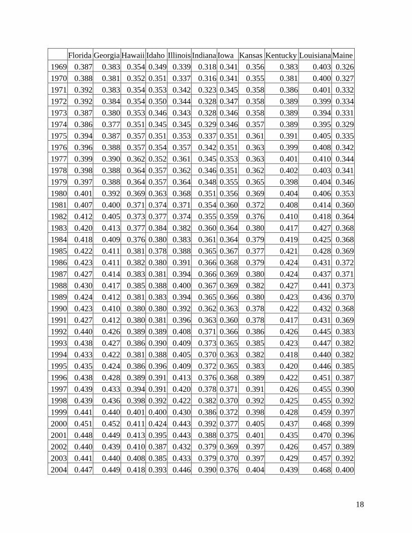
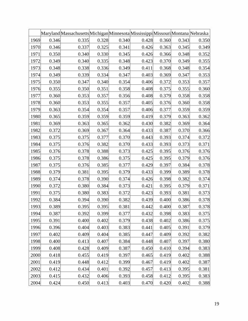
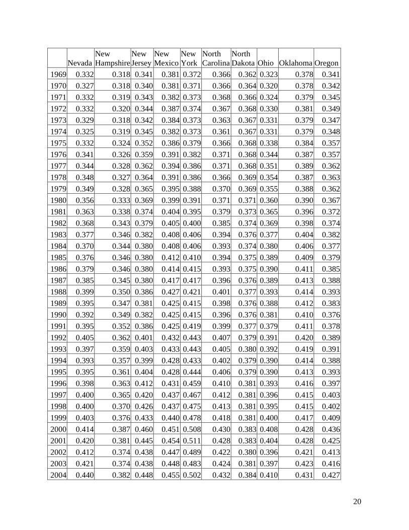
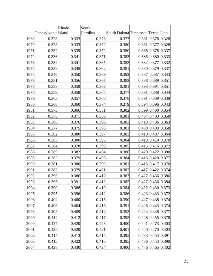
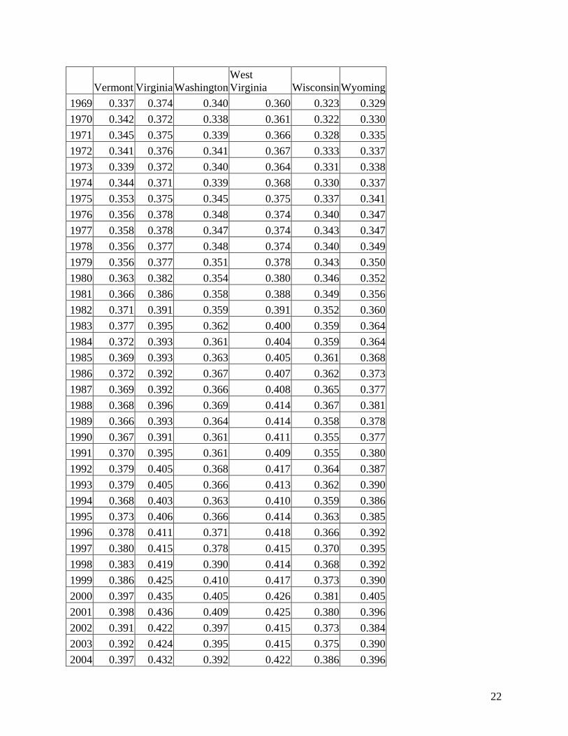
lower than .75. With only four overlapping years of data, there is some fear of spurious correlation, but the consistency of the results across 51 cross-sectional units of analysis is nonetheless impressive. These temporal correlations, while compelling, may be confounded by general secular trends. However, the Theil-based estimates are robust cross-sectionally as well as temporally. Because the states vary in their industrial mix, and by extension the number of sectors, the pay inequality values are not directly comparable from one state to the next.13 However, we can get roughly consistent measures for changes over time by looking at the percentage change in pay inequality from 1969 to 1999 and comparing this to the percentage changes in income inequality over the same period. The cross-sectional correlation of the two measures is .80. Though the series are not perfectly matched, they certainly bear a strong family resemblance. If the pay inequality and income inequality measures are representing the same phenomena, we would expect the regressions of the Theil-based values on the Gini coefficients for each state to have high R2 values (albeit with only 2 degrees of freedom) and small residuals. Further, we would expect that the cross-sectional correlations across states between the predicted values and the actual Gini coefficient values to be high. These conditions are all met. Finally, when we see a significant year-to-year fluctuation in a state’s level of inequality, our method permits us to examine the underlying sectoral data for an explanation. For instance, inequality shot up in New York from 1999 to 2000. Since New York is a center of world finance, one might look to the financial services sector to see if its changing wages or employment levels are driving the rise in inequality. The underlying Theil elements, which break out the effects of the financial sector, confirm this hypothesis. From 1999 to 2000 the average salary for New York’s 200,000 security and commodity brokers shot up from $188,595 to $238,868, while the average salary across the state saw a much more modest gain from $41,614 to $44,737. In this manner, we can use the sectoral data to confirm or challenge conventional wisdom, a luxury we may not have with micro data. Exploring the Yearly State Estimates From 1969 to 2004, our estimate of Gini coefficient of family income increased for every state. The state average, not weighting by population, was .356 in 1969 and .427 in 2004. The average increase was 20%, with the range from a 6% increase in North Dakota to a 46% increase in Connecticut. Appendix 2 provides all of the state approximations of Gini coefficients of family income in tabular format. Appendix 3 compares our measures with those of Langer (1999). Despite the fact that inequality grew everywhere, states and regions did see different patterns of change.

5

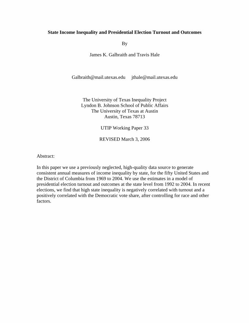
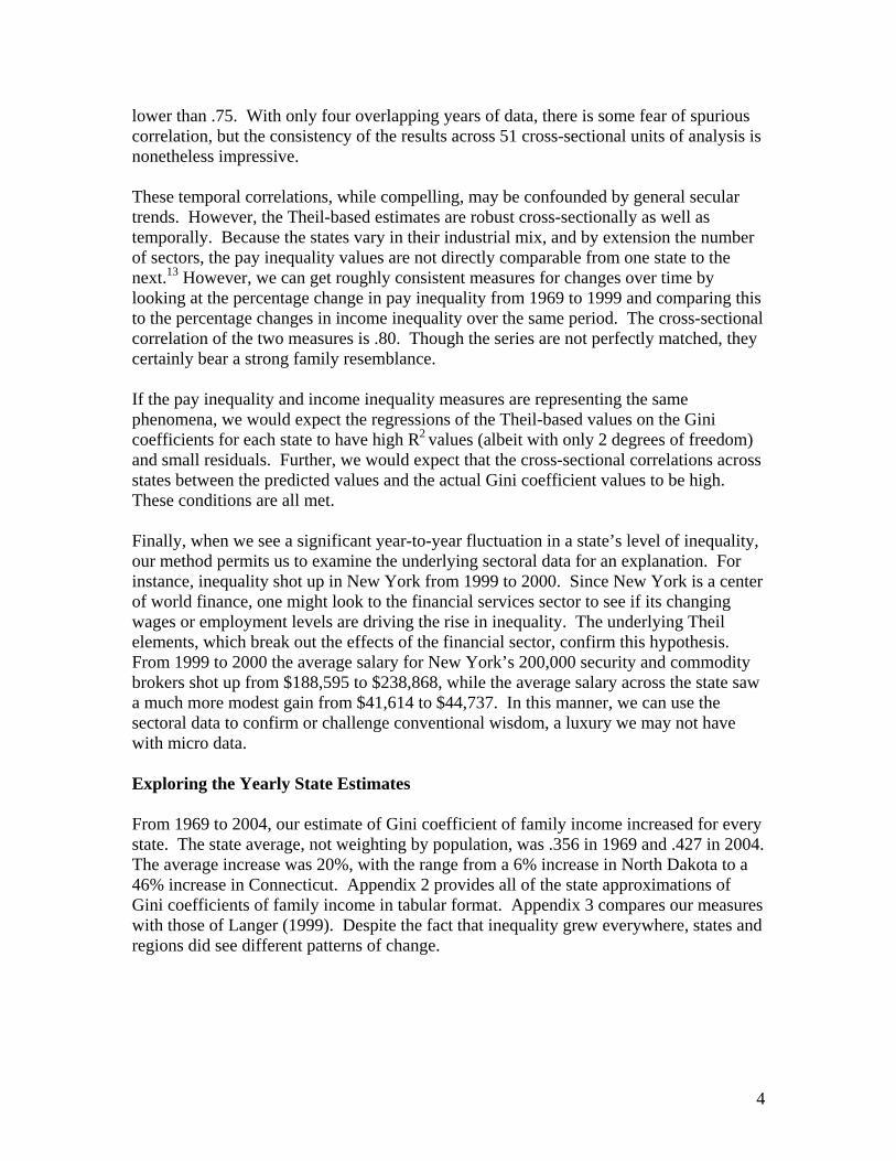
Figure 1. State Gini Coefficient Approximations for Selected States 1969 - 2004

0.3

0.35

0.4

0.45

0.5

0.55

0.6

1968 1973 1978 1983 1988 1993 1998 2003

Alaska California DC Iowa New York

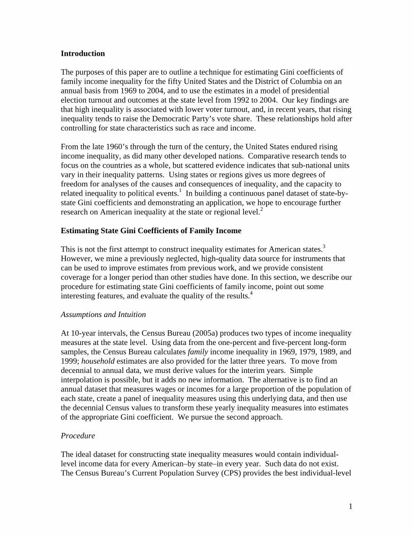
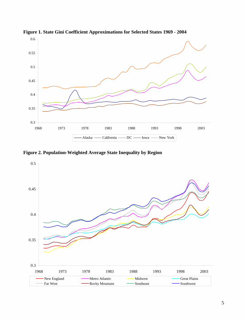
Figure 2. Population-Weighted Average State Inequality by Region

0.3

0.35

0.4

0.45

0.5

1968 1973 1978 1983 1988 1993 1998 2003

New England Metro Atlantic Midwest Great PlainsFar West Rocky Mountain Southeast Southwest

6

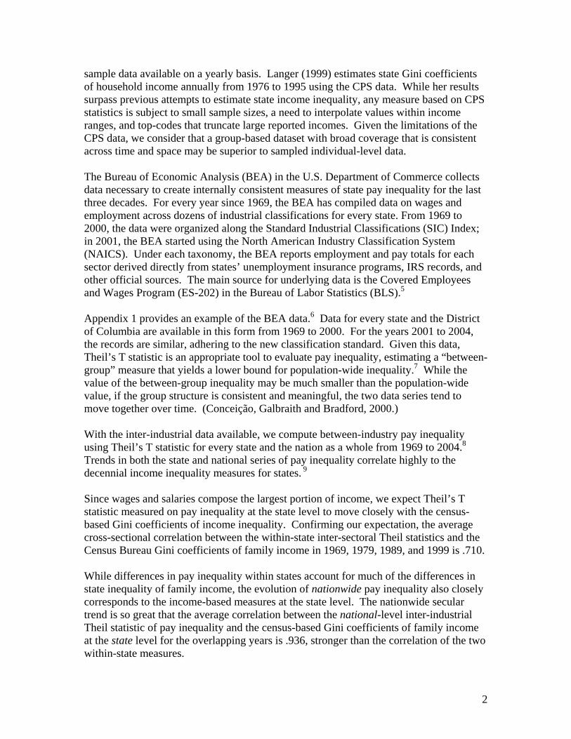
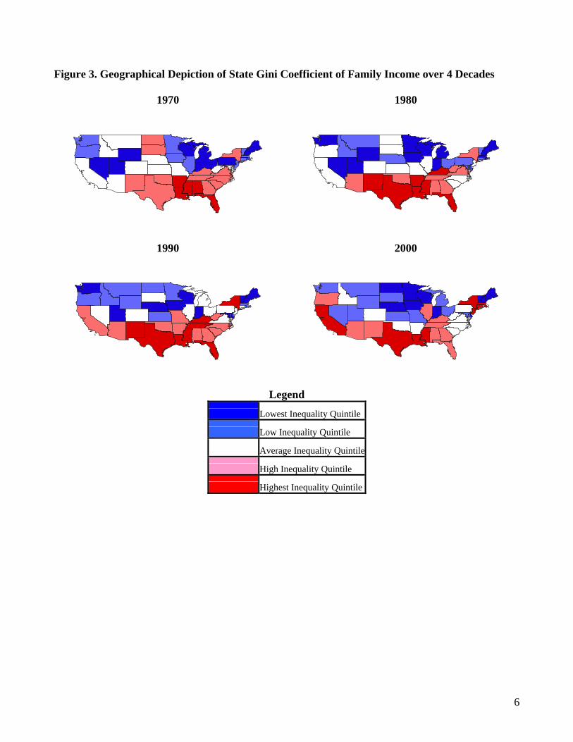
Figure 3. Geographical Depiction of State Gini Coefficient of Family Income over 4 Decades

1970

1980

1990

2000

Legend

Lowest Inequality Quintile

Low Inequality Quintile

Average Inequality Quintile

High Inequality Quintile

Highest Inequality Quintile

7

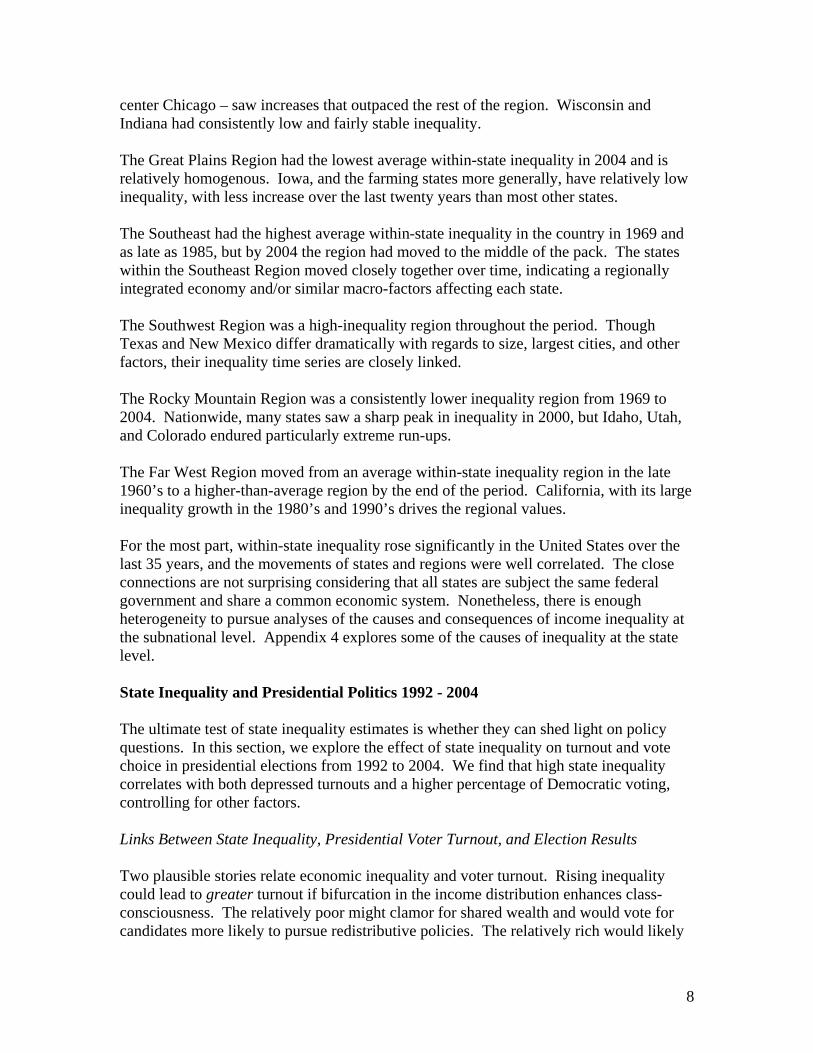
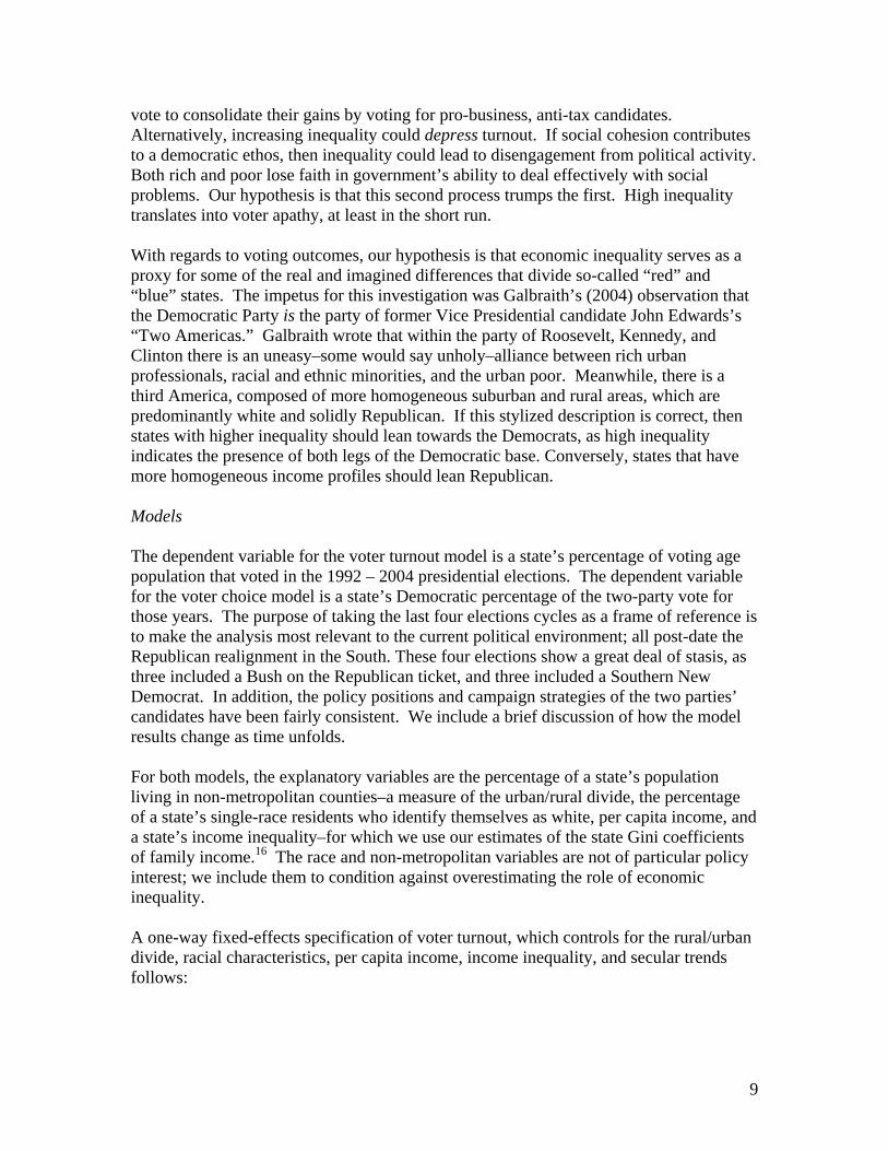
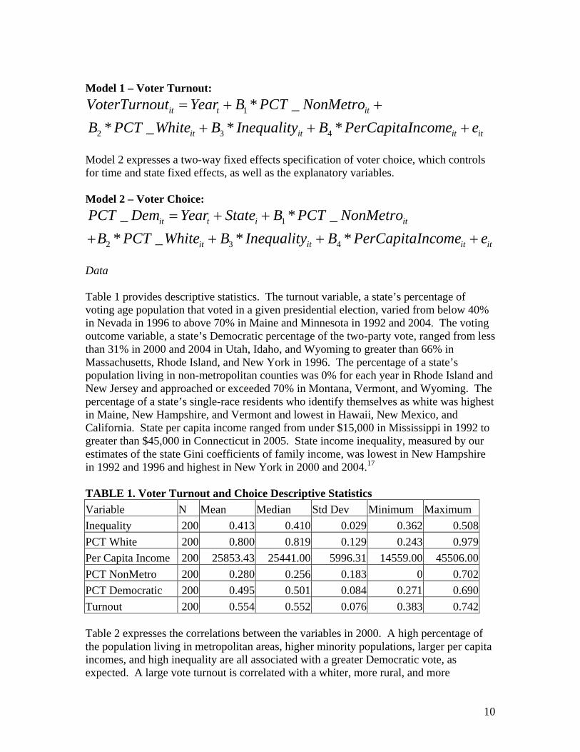
Figure 1 highlights the variation in the evolution of state income inequality for selected states from 1969 to 2004.14 In Washington D.C., the disparity of urban poverty in contrast with high paying jobs associated with the federal government helps explain persistently high inequality. Indeed, the District of Columbia is unique in its inequality profile and other features; so much so that researchers must show caution in including the nation’s capital as a de facto fifty-first state. California and New York saw higher than average inequality growth during this period. Volatile finance, entertainment, and high technology sectors are likely culprits. Geography is also an important force in both states, where salaries and incomes in and around New York City, Los Angeles, San Diego, and the Bay Area reflect a higher cost of living than in the hinterlands. Iowa is shown as an example of states with much lower inequality and less change. Alaska, with its sharp rise and decline in inequality in the mid to late 1970’s, presents another unique case. Unless there is an error in the data, something remarkable must have happened in Alaska in 1975 and 1976, causing a large run-up in inequality that virtually disappeared by 1978. The industrial data solves the mystery – it was the construction of the Tran-Alaska pipeline. The number of heavy construction contractors soared from 6,174 in 1974 to 21,176 in 1976 then plummeted to 3,464 in 1978. Throughout this period, heavy construction contractors received a salary approximately 2.5 times greater than the average Alaskan. Thus, the inequality spike was real, short-lived, and well explained by the appropriate historical data. Figure 2 plots weighted averages of the state measures across regions – the expected value of within-state inequality for a typical person living in the region.15 Regional inequality, distinct from state inequality, is a topic we hope to address in future research. Figure 3 captures the general rankings of all the states at four points in time. From 1969 to 2004, New England became more heterogeneous with regards to within-state income inequality, while the region as a whole evolved from a lower-inequality region to a higher-inequality region. Connecticut, with its close proximity to New York City, and Massachusetts, with Boston as the relatively rich regional center, drove the inequality increases. New Hampshire, Maine, and Vermont remain consistently among the most equal states in the nation. Inequality in New York State and, especially, Washington D.C. was persistently higher than for the rest of the Metro Atlantic Region. On the whole, the Metro Atlantic Region moved from a region with average statewide inequality to the most unequal region in the country. Even within this environment, Delaware stood out as a low inequality state, and one that did not see steep inequality rises in 1999 and 2000, which were felt in almost every other state. Average within-state inequality in the Midwest remained relatively low throughout the 1969 to 2004 period. Paralleling New York and Massachusetts, Illinois – with regional

8

center Chicago – saw increases that outpaced the rest of the region. Wisconsin and Indiana had consistently low and fairly stable inequality. The Great Plains Region had the lowest average within-state inequality in 2004 and is relatively homogenous. Iowa, and the farming states more generally, have relatively low inequality, with less increase over the last twenty years than most other states. The Southeast had the highest average within-state inequality in the country in 1969 and as late as 1985, but by 2004 the region had moved to the middle of the pack. The states within the Southeast Region moved closely together over time, indicating a regionally integrated economy and/or similar macro-factors affecting each state. The Southwest Region was a high-inequality region throughout the period. Though Texas and New Mexico differ dramatically with regards to size, largest cities, and other factors, their inequality time series are closely linked. The Rocky Mountain Region was a consistently lower inequality region from 1969 to 2004. Nationwide, many states saw a sharp peak in inequality in 2000, but Idaho, Utah, and Colorado endured particularly extreme run-ups. The Far West Region moved from an average within-state inequality region in the late 1960’s to a higher-than-average region by the end of the period. California, with its large inequality growth in the 1980’s and 1990’s drives the regional values. For the most part, within-state inequality rose significantly in the United States over the last 35 years, and the movements of states and regions were well correlated. The close connections are not surprising considering that all states are subject the same federal government and share a common economic system. Nonetheless, there is enough heterogeneity to pursue analyses of the causes and consequences of income inequality at the subnational level. Appendix 4 explores some of the causes of inequality at the state level. State Inequality and Presidential Politics 1992 - 2004 The ultimate test of state inequality estimates is whether they can shed light on policy questions. In this section, we explore the effect of state inequality on turnout and vote choice in presidential elections from 1992 to 2004. We find that high state inequality correlates with both depressed turnouts and a higher percentage of Democratic voting, controlling for other factors. Links Between State Inequality, Presidential Voter Turnout, and Election Results Two plausible stories relate economic inequality and voter turnout. Rising inequality could lead to greater turnout if bifurcation in the income distribution enhances class-consciousness. The relatively poor might clamor for shared wealth and would vote for candidates more likely to pursue redistributive policies. The relatively rich would likely

9

vote to consolidate their gains by voting for pro-business, anti-tax candidates. Alternatively, increasing inequality could depress turnout. If social cohesion contributes to a democratic ethos, then inequality could lead to disengagement from political activity. Both rich and poor lose faith in government’s ability to deal effectively with social problems. Our hypothesis is that this second process trumps the first. High inequality translates into voter apathy, at least in the short run. With regards to voting outcomes, our hypothesis is that economic inequality serves as a proxy for some of the real and imagined differences that divide so-called “red” and “blue” states. The impetus for this investigation was Galbraith’s (2004) observation that the Democratic Party is the party of former Vice Presidential candidate John Edwards’s “Two Americas.” Galbraith wrote that within the party of Roosevelt, Kennedy, and Clinton there is an uneasy–some would say unholy–alliance between rich urban professionals, racial and ethnic minorities, and the urban poor. Meanwhile, there is a third America, composed of more homogeneous suburban and rural areas, which are predominantly white and solidly Republican. If this stylized description is correct, then states with higher inequality should lean towards the Democrats, as high inequality indicates the presence of both legs of the Democratic base. Conversely, states that have more homogeneous income profiles should lean Republican. Models The dependent variable for the voter turnout model is a state’s percentage of voting age population that voted in the 1992 – 2004 presidential elections. The dependent variable for the voter choice model is a state’s Democratic percentage of the two-party vote for those years. The purpose of taking the last four elections cycles as a frame of reference is to make the analysis most relevant to the current political environment; all post-date the Republican realignment in the South. These four elections show a great deal of stasis, as three included a Bush on the Republican ticket, and three included a Southern New Democrat. In addition, the policy positions and campaign strategies of the two parties’ candidates have been fairly consistent. We include a brief discussion of how the model results change as time unfolds. For both models, the explanatory variables are the percentage of a state’s population living in non-metropolitan counties–a measure of the urban/rural divide, the percentage of a state’s single-race residents who identify themselves as white, per capita income, and a state’s income inequality–for which we use our estimates of the state Gini coefficients of family income.16 The race and non-metropolitan variables are not of particular policy interest; we include them to condition against overestimating the role of economic inequality. A one-way fixed-effects specification of voter turnout, which controls for the rural/urban divide, racial characteristics, per capita income, income inequality, and secular trends follows:

10

Model 1 – Voter Turnout:

1

2 3 4

* _* _ * *

it t it

it it it it

VoterTurnout Year B PCT NonMetroB PCT White B Inequality B PerCapitaIncome e

= + +

+ + +

Model 2 expresses a two-way fixed effects specification of voter choice, which controls for time and state fixed effects, as well as the explanatory variables. Model 2 – Voter Choice:

1

2 3 4

_ * _* _ * *

it t i it

it it it it

PCT Dem Year State B PCT NonMetroB PCT White B Inequality B PerCapitaIncome e

= + +

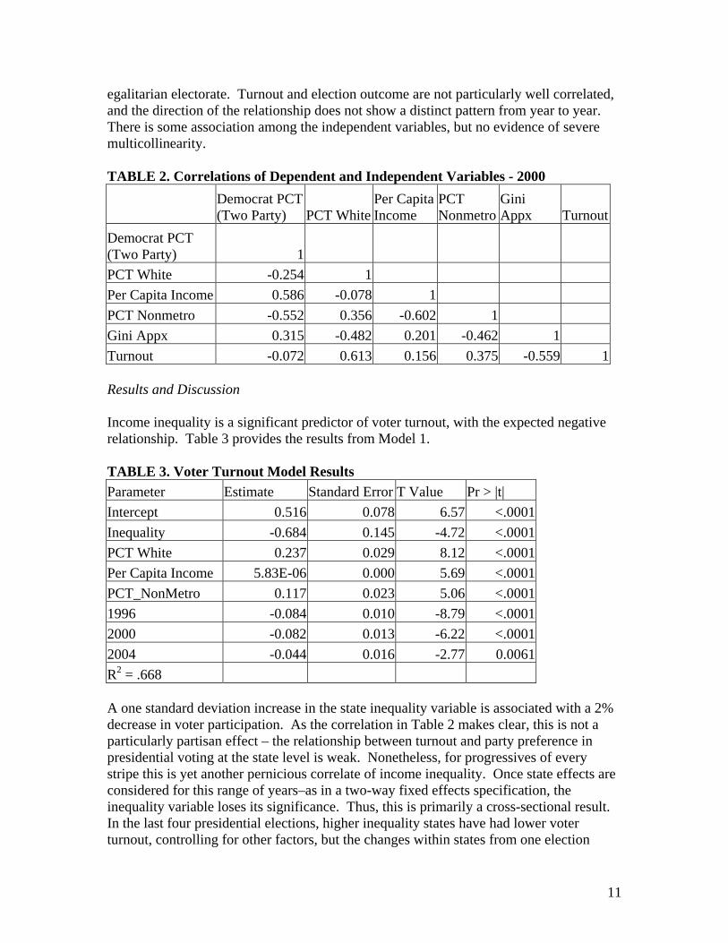
+ + + + Data Table 1 provides descriptive statistics. The turnout variable, a state’s percentage of voting age population that voted in a given presidential election, varied from below 40% in Nevada in 1996 to above 70% in Maine and Minnesota in 1992 and 2004. The voting outcome variable, a state’s Democratic percentage of the two-party vote, ranged from less than 31% in 2000 and 2004 in Utah, Idaho, and Wyoming to greater than 66% in Massachusetts, Rhode Island, and New York in 1996. The percentage of a state’s population living in non-metropolitan counties was 0% for each year in Rhode Island and New Jersey and approached or exceeded 70% in Montana, Vermont, and Wyoming. The percentage of a state’s single-race residents who identify themselves as white was highest in Maine, New Hampshire, and Vermont and lowest in Hawaii, New Mexico, and California. State per capita income ranged from under $15,000 in Mississippi in 1992 to greater than $45,000 in Connecticut in 2005. State income inequality, measured by our estimates of the state Gini coefficients of family income, was lowest in New Hampshire in 1992 and 1996 and highest in New York in 2000 and 2004.17 TABLE 1. Voter Turnout and Choice Descriptive Statistics Variable N Mean Median Std Dev Minimum Maximum Inequality 200 0.413 0.410 0.029 0.362 0.508PCT White 200 0.800 0.819 0.129 0.243 0.979Per Capita Income 200 25853.43 25441.00 5996.31 14559.00 45506.00PCT NonMetro 200 0.280 0.256 0.183 0 0.702PCT Democratic 200 0.495 0.501 0.084 0.271 0.690Turnout 200 0.554 0.552 0.076 0.383 0.742 Table 2 expresses the correlations between the variables in 2000. A high percentage of the population living in metropolitan areas, higher minority populations, larger per capita incomes, and high inequality are all associated with a greater Democratic vote, as expected. A large vote turnout is correlated with a whiter, more rural, and more

11

egalitarian electorate. Turnout and election outcome are not particularly well correlated, and the direction of the relationship does not show a distinct pattern from year to year. There is some association among the independent variables, but no evidence of severe multicollinearity. TABLE 2. Correlations of Dependent and Independent Variables - 2000

Democrat PCT (Two Party) PCT White

Per Capita Income

PCT Nonmetro

Gini Appx Turnout

Democrat PCT (Two Party) 1 PCT White -0.254 1 Per Capita Income 0.586 -0.078 1 PCT Nonmetro -0.552 0.356 -0.602 1 Gini Appx 0.315 -0.482 0.201 -0.462 1 Turnout -0.072 0.613 0.156 0.375 -0.559 1 Results and Discussion Income inequality is a significant predictor of voter turnout, with the expected negative relationship. Table 3 provides the results from Model 1. TABLE 3. Voter Turnout Model Results Parameter Estimate Standard Error T Value Pr > |t| Intercept 0.516 0.078 6.57 <.0001 Inequality -0.684 0.145 -4.72 <.0001 PCT White 0.237 0.029 8.12 <.0001 Per Capita Income 5.83E-06 0.000 5.69 <.0001 PCT_NonMetro 0.117 0.023 5.06 <.0001 1996 -0.084 0.010 -8.79 <.0001 2000 -0.082 0.013 -6.22 <.0001 2004 -0.044 0.016 -2.77 0.0061 R2 = .668 A one standard deviation increase in the state inequality variable is associated with a 2% decrease in voter participation. As the correlation in Table 2 makes clear, this is not a particularly partisan effect – the relationship between turnout and party preference in presidential voting at the state level is weak. Nonetheless, for progressives of every stripe this is yet another pernicious correlate of income inequality. Once state effects are considered for this range of years–as in a two-way fixed effects specification, the inequality variable loses its significance. Thus, this is primarily a cross-sectional result. In the last four presidential elections, higher inequality states have had lower voter turnout, controlling for other factors, but the changes within states from one election

12

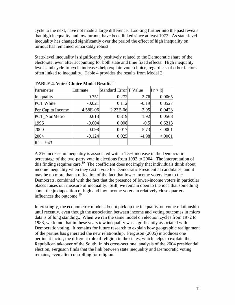
cycle to the next, have not made a large difference. Looking further into the past reveals that high inequality and low turnout have been linked since at least 1972. As state-level inequality has changed significantly over the period the effect of high inequality on turnout has remained remarkably robust. State-level inequality is significantly positively related to the Democratic share of the electorate, even after accounting for both state and time fixed effects. High inequality levels and cycle-to-cycle increases help explain voter choice, regardless of other factors often linked to inequality. Table 4 provides the results from Model 2. TABLE 4. Voter Choice Model Results18 Parameter Estimate Standard Error T Value Pr > |t| Inequality 0.751 0.272 2.76 0.0065 PCT White -0.021 0.112 -0.19 0.8527 Per Capita Income 4.58E-06 2.23E-06 2.05 0.0423 PCT_NonMetro 0.613 0.319 1.92 0.0568 1996 -0.004 0.008 -0.5 0.6213 2000 -0.098 0.017 -5.73 <.0001 2004 -0.124 0.025 -4.98 <.0001 R2 = .943 A 2% increase in inequality is associated with a 1.5% increase in the Democratic percentage of the two-party vote in elections from 1992 to 2004. The interpretation of this finding requires care.19 The coefficient does not imply that individuals think about income inequality when they cast a vote for Democratic Presidential candidates, and it may be no more than a reflection of the fact that lower income voters lean to the Democrats, combined with the fact that the presence of lower-income voters in particular places raises our measure of inequality. Still, we remain open to the idea that something about the juxtaposition of high and low income voters in relatively close quarters influences the outcome.20 Interestingly, the econometric models do not pick up the inequality-outcome relationship until recently, even though the association between income and voting outcomes in micro data is of long standing.. When we ran the same model on election cycles from 1972 to 1988, we found that in these years low inequality was significantly associated with Democratic voting. It remains for future research to explain how geographic realignment of the parties has generated the new relationship. Ferguson (2005) introduces one pertinent factor, the different role of religion in the states, which helps to explain the Republican takeover of the South. In his cross-sectional analysis of the 2004 presidential election, Ferguson finds that the link between state inequality and Democratic voting remains, even after controlling for religion.

13

Final Thoughts Many studies of inequality in the United States have centered on the causes and effects of an increasingly inegalitarian wage and income structure at the national level, leaving questions about state and local trends largely unanswered. The dataset we introduce here, which will be available on the UTIP web-site, will facilitate additional research on wage and income inequality dynamics within and between states. We believe it can assist the analysis of many public policy issues. Our application of state inequality to issues of voter turnout and choice in presidential elections shows the promise of this line of inquiry, as well as providing insight into a vital issue in modern American politics.

14

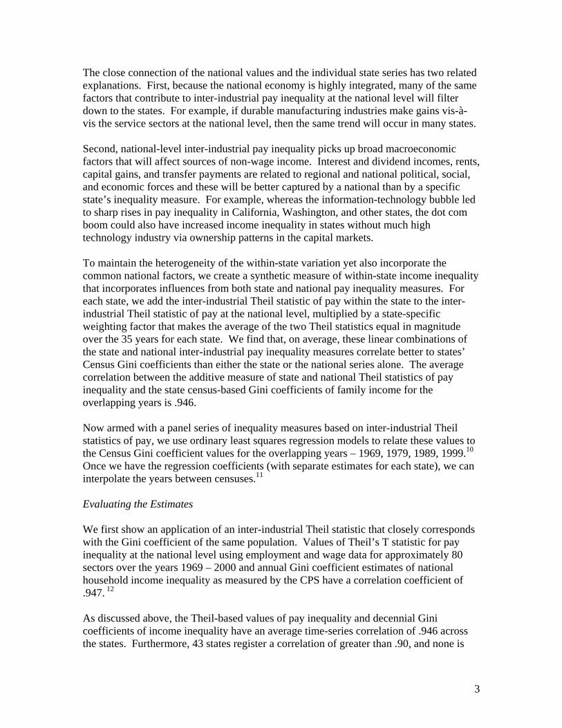
APPENDIX 1 – Example of the Raw Data Idaho, 1995 Item Employment

Total Wages and Salaries (in 1,000s)

Total Private Employment and Wage and Salaries 527928 9078776 Agricultural services, forestry, fishing and other 15615 146353 Agricultural services 14303 135566 Forestry, fishing, and other 1312 10787 Forestry 1009 9935 Fishing 303 852 Other 0 0 Mining 3551 95527 Metal mining 1957 (D) Coal mining (L) (D) Oil and gas extraction 394 (D) Nonmetallic minerals, except fuels 1191 31093 Construction 46851 814182 General building contractors 9880 169016 Heavy construction contractors 6570 205185 Special trade contractors 30401 439981 Manufacturing 76773 2321265 Durable goods 46429 1560600 Lumber and wood products 16858 442606 Furniture and fixtures 1436 23308 Stone, clay, and glass products 1670 37591 Primary metal industries 261 6773 Fabricated metal products 3192 72369 Industrial machinery and equipment 9681 390629 Electronic and other electric equipment 8929 500179 Motor vehicles and equipment 907 23736 Other transportation equipment 1409 30663 Instruments and related products 477 13473 Miscellaneous manufacturing industries 1609 19273 Ordnance (N) (N) Nondurable goods 30344 760665 Food and kindred products 17683 434182 Tobacco products (L) 0 Textile mill products 54 718 Apparel and other textile products 778 5945

15

Paper and allied products 2201 (D) Printing and publishing 5582 (D) Chemicals and allied products 2522 93698 Petroleum and coal products 25 607 Rubber and miscellaneous plastics products 1220 23424 Leather and leather products 273 2541 Transportation and public utilities 28173 681490 Railroad transportation 1884 94948 Trucking and warehousing 12197 205211 Water transportation 238 (D) Other transportation 5498 (D) Local and interurban passenger transit 1461 (D) Transportation by air 2527 60636 Pipelines, except natural gas 25 (D) Transportation services 1485 20497 Communications 4152 122041 Electric, gas, and sanitary services 4204 158877 Wholesale trade 30524 701621 Retail trade 118432 1286113 Building materials and garden equipment 6507 110773 General merchandise stores 10727 132434 Food stores 16569 252011 Automotive dealers and service stations 14283 281970 Apparel and accessory stores 4134 36469 Home furniture and furnishings stores 5291 77207 Eating and drinking places 35903 276159 Miscellaneous retail 25018 119090 Finance, insurance, and real estate 41978 567248 Depository and nondepository institutions 9027 (D) Other finance, insurance, and real estate 32951 (D) Security and commodity brokers 1088 36702 Insurance carriers 3612 105621 Insurance agents, brokers, and services 5700 76760 Real estate 17090 71059 Combined real estate, insurance, etc. (N) (N) Holding and other investment offices 5461 (D) Services 166031 2464977 Hotels and other lodging places 9158 95331 Personal services 11536 52751

16

Private households 4245 31746 Business services 27841 248677 Automotive repair, services, and parking 8167 79269 Miscellaneous repair services 4222 30217 Amusement and recreation services 9410 73236 Motion pictures 1883 12067 Health services 34337 789208 Legal services 4254 100095 Educational services 8404 78174 Social services 9509 116368 Museums, botanical, zoological gardens 70 813 Membership organizations 5372 88543 Engineering and management services 21979 654925 Miscellaneous services 5644 13557 Government and government enterprises 104706 2338356 Federal, civilian 12986 455939 Military 9705 160614 State and local 82015 1721803 State government 25945 606951 Local government 56070 1114852

(D) Not shown to avoid disclosure of confidential information, but the estimates for this item are included in the total.

(L) Less than $50,000, but the estimates for this item are included in the total.

(N) Data not available for this year.

17

APPENDIX 2 – State Gini Estimates 1969 – 2004 Alabama Alaska Arizona Arkansas California Colorado Connecticut Delaware DC 1969 0.395 0.366 0.356 0.401 0.360 0.347 0.337 0.344 0.4261970 0.390 0.360 0.355 0.400 0.361 0.346 0.337 0.341 0.4271971 0.395 0.359 0.361 0.403 0.364 0.348 0.339 0.347 0.4321972 0.394 0.354 0.362 0.403 0.365 0.349 0.343 0.346 0.4311973 0.385 0.350 0.359 0.398 0.362 0.347 0.343 0.343 0.4261974 0.381 0.366 0.359 0.397 0.361 0.348 0.344 0.346 0.4221975 0.392 0.401 0.371 0.402 0.371 0.356 0.352 0.351 0.4261976 0.390 0.417 0.375 0.401 0.373 0.360 0.355 0.353 0.4281977 0.392 0.390 0.379 0.401 0.374 0.364 0.358 0.358 0.4291978 0.384 0.371 0.378 0.391 0.372 0.361 0.360 0.355 0.4291979 0.385 0.369 0.376 0.389 0.376 0.361 0.361 0.358 0.4301980 0.389 0.372 0.382 0.397 0.379 0.367 0.366 0.364 0.4311981 0.396 0.375 0.389 0.400 0.385 0.373 0.372 0.367 0.4381982 0.400 0.376 0.389 0.403 0.390 0.375 0.375 0.371 0.4531983 0.407 0.376 0.394 0.409 0.398 0.379 0.380 0.377 0.4611984 0.407 0.374 0.392 0.405 0.396 0.376 0.378 0.382 0.4561985 0.409 0.374 0.396 0.409 0.400 0.381 0.380 0.388 0.4641986 0.405 0.377 0.397 0.413 0.406 0.383 0.381 0.385 0.4821987 0.411 0.378 0.403 0.415 0.414 0.386 0.379 0.382 0.4831988 0.420 0.379 0.410 0.415 0.418 0.389 0.388 0.378 0.5041989 0.414 0.382 0.410 0.411 0.410 0.386 0.381 0.376 0.4941990 0.411 0.376 0.408 0.408 0.408 0.385 0.383 0.373 0.4941991 0.414 0.377 0.412 0.408 0.411 0.385 0.383 0.374 0.4971992 0.431 0.381 0.422 0.417 0.425 0.393 0.400 0.379 0.5121993 0.429 0.379 0.420 0.417 0.428 0.393 0.405 0.381 0.5161994 0.421 0.380 0.414 0.412 0.424 0.388 0.399 0.381 0.5151995 0.428 0.381 0.416 0.413 0.430 0.392 0.409 0.384 0.5291996 0.430 0.383 0.418 0.416 0.437 0.396 0.418 0.388 0.5371997 0.432 0.385 0.420 0.417 0.442 0.398 0.432 0.391 0.5441998 0.432 0.383 0.423 0.417 0.446 0.402 0.440 0.389 0.5481999 0.437 0.382 0.428 0.419 0.463 0.414 0.451 0.390 0.5592000 0.450 0.391 0.441 0.427 0.489 0.430 0.468 0.397 0.5942001 0.449 0.392 0.441 0.428 0.470 0.423 0.482 0.400 0.5752002 0.437 0.388 0.430 0.420 0.454 0.410 0.465 0.391 0.5622003 0.440 0.384 0.430 0.421 0.455 0.413 0.471 0.392 0.5622004 0.454 0.389 0.439 0.427 0.467 0.423 0.492 0.396 0.580

18

Florida Georgia Hawaii Idaho Illinois Indiana Iowa Kansas Kentucky Louisiana Maine1969 0.387 0.383 0.354 0.349 0.339 0.318 0.341 0.356 0.383 0.403 0.3261970 0.388 0.381 0.352 0.351 0.337 0.316 0.341 0.355 0.381 0.400 0.3271971 0.392 0.383 0.354 0.353 0.342 0.323 0.345 0.358 0.386 0.401 0.3321972 0.392 0.384 0.354 0.350 0.344 0.328 0.347 0.358 0.389 0.399 0.3341973 0.387 0.380 0.353 0.346 0.343 0.328 0.346 0.358 0.389 0.394 0.3311974 0.386 0.377 0.351 0.345 0.345 0.329 0.346 0.357 0.389 0.395 0.3291975 0.394 0.387 0.357 0.351 0.353 0.337 0.351 0.361 0.391 0.405 0.3351976 0.396 0.388 0.357 0.354 0.357 0.342 0.351 0.363 0.399 0.408 0.3421977 0.399 0.390 0.362 0.352 0.361 0.345 0.353 0.363 0.401 0.410 0.3441978 0.398 0.388 0.364 0.357 0.362 0.346 0.351 0.362 0.402 0.403 0.3411979 0.397 0.388 0.364 0.357 0.364 0.348 0.355 0.365 0.398 0.404 0.3461980 0.401 0.392 0.369 0.363 0.368 0.351 0.356 0.369 0.404 0.406 0.3531981 0.407 0.400 0.371 0.374 0.371 0.354 0.360 0.372 0.408 0.414 0.3601982 0.412 0.405 0.373 0.377 0.374 0.355 0.359 0.376 0.410 0.418 0.3641983 0.420 0.413 0.377 0.384 0.382 0.360 0.364 0.380 0.417 0.427 0.3681984 0.418 0.409 0.376 0.380 0.383 0.361 0.364 0.379 0.419 0.425 0.3681985 0.422 0.411 0.381 0.378 0.388 0.365 0.367 0.377 0.421 0.428 0.3691986 0.423 0.411 0.382 0.380 0.391 0.366 0.368 0.379 0.424 0.431 0.3721987 0.427 0.414 0.383 0.381 0.394 0.366 0.369 0.380 0.424 0.437 0.3711988 0.430 0.417 0.385 0.388 0.400 0.367 0.369 0.382 0.427 0.441 0.3731989 0.424 0.412 0.381 0.383 0.394 0.365 0.366 0.380 0.423 0.436 0.3701990 0.423 0.410 0.380 0.380 0.392 0.362 0.363 0.378 0.422 0.432 0.3681991 0.427 0.412 0.380 0.381 0.396 0.363 0.360 0.378 0.417 0.431 0.3691992 0.440 0.426 0.389 0.389 0.408 0.371 0.366 0.386 0.426 0.445 0.3831993 0.438 0.427 0.386 0.390 0.409 0.373 0.365 0.385 0.423 0.447 0.3821994 0.433 0.422 0.381 0.388 0.405 0.370 0.363 0.382 0.418 0.440 0.3821995 0.435 0.424 0.386 0.396 0.409 0.372 0.365 0.383 0.420 0.446 0.3851996 0.438 0.428 0.389 0.391 0.413 0.376 0.368 0.389 0.422 0.451 0.3871997 0.439 0.433 0.394 0.391 0.420 0.378 0.371 0.391 0.426 0.455 0.3901998 0.439 0.436 0.398 0.392 0.422 0.382 0.370 0.392 0.425 0.455 0.3921999 0.441 0.440 0.401 0.400 0.430 0.386 0.372 0.398 0.428 0.459 0.3972000 0.451 0.452 0.411 0.424 0.443 0.392 0.377 0.405 0.437 0.468 0.3992001 0.448 0.449 0.413 0.395 0.443 0.388 0.375 0.401 0.435 0.470 0.3962002 0.440 0.439 0.410 0.387 0.432 0.379 0.369 0.397 0.426 0.457 0.3892003 0.441 0.440 0.408 0.385 0.433 0.379 0.370 0.397 0.429 0.457 0.3922004 0.447 0.449 0.418 0.393 0.446 0.390 0.376 0.404 0.439 0.468 0.400

19

Maryland Massachusetts Michigan Minnesota Mississippi Missouri Montana Nebraska1969 0.346 0.335 0.328 0.340 0.428 0.360 0.343 0.3501970 0.346 0.337 0.325 0.341 0.426 0.363 0.345 0.3491971 0.350 0.340 0.330 0.345 0.426 0.366 0.348 0.3521972 0.349 0.340 0.335 0.348 0.423 0.370 0.349 0.3551973 0.348 0.338 0.336 0.349 0.411 0.368 0.348 0.3541974 0.349 0.339 0.334 0.347 0.403 0.369 0.347 0.3531975 0.350 0.347 0.340 0.354 0.406 0.372 0.353 0.3571976 0.355 0.350 0.351 0.358 0.408 0.375 0.355 0.3601977 0.360 0.353 0.357 0.356 0.408 0.379 0.358 0.3581978 0.360 0.353 0.355 0.357 0.405 0.376 0.360 0.3581979 0.363 0.354 0.354 0.357 0.406 0.377 0.359 0.3591980 0.365 0.359 0.359 0.359 0.419 0.379 0.363 0.3621981 0.369 0.363 0.365 0.362 0.430 0.382 0.369 0.3641982 0.372 0.369 0.367 0.364 0.433 0.387 0.370 0.3661983 0.375 0.375 0.377 0.370 0.443 0.393 0.374 0.3721984 0.375 0.376 0.382 0.370 0.433 0.393 0.373 0.3711985 0.376 0.378 0.388 0.373 0.425 0.395 0.376 0.3761986 0.375 0.378 0.386 0.375 0.425 0.395 0.379 0.3761987 0.375 0.376 0.385 0.377 0.429 0.397 0.384 0.3781988 0.379 0.381 0.395 0.379 0.433 0.399 0.389 0.3781989 0.374 0.378 0.390 0.374 0.426 0.398 0.382 0.3741990 0.372 0.380 0.384 0.373 0.421 0.395 0.379 0.3711991 0.375 0.380 0.383 0.372 0.423 0.393 0.381 0.3731992 0.384 0.394 0.390 0.382 0.439 0.400 0.386 0.3781993 0.389 0.395 0.395 0.381 0.442 0.400 0.387 0.3781994 0.387 0.392 0.399 0.377 0.432 0.398 0.383 0.3751995 0.391 0.400 0.402 0.379 0.438 0.402 0.386 0.3751996 0.396 0.404 0.403 0.383 0.441 0.405 0.391 0.3791997 0.402 0.409 0.404 0.385 0.447 0.409 0.392 0.3821998 0.400 0.413 0.407 0.384 0.448 0.407 0.397 0.3801999 0.408 0.428 0.409 0.387 0.450 0.410 0.394 0.3832000 0.418 0.455 0.419 0.397 0.465 0.419 0.402 0.3882001 0.419 0.448 0.412 0.399 0.467 0.419 0.402 0.3872002 0.412 0.434 0.401 0.392 0.457 0.413 0.395 0.3812003 0.415 0.432 0.406 0.393 0.458 0.412 0.395 0.3832004 0.424 0.450 0.413 0.403 0.470 0.420 0.402 0.388

20

Nevada New Hampshire

New Jersey

New Mexico

New York

North Carolina

North Dakota Ohio Oklahoma Oregon

1969 0.332 0.318 0.341 0.381 0.372 0.366 0.362 0.323 0.378 0.3411970 0.327 0.318 0.340 0.381 0.371 0.366 0.364 0.320 0.378 0.3421971 0.332 0.319 0.343 0.382 0.373 0.368 0.366 0.324 0.379 0.3451972 0.332 0.320 0.344 0.387 0.374 0.367 0.368 0.330 0.381 0.3491973 0.329 0.318 0.342 0.384 0.373 0.363 0.367 0.331 0.379 0.3471974 0.325 0.319 0.345 0.382 0.373 0.361 0.367 0.331 0.379 0.3481975 0.332 0.324 0.352 0.386 0.379 0.366 0.368 0.338 0.384 0.3571976 0.341 0.326 0.359 0.391 0.382 0.371 0.368 0.344 0.387 0.3571977 0.344 0.328 0.362 0.394 0.386 0.371 0.368 0.351 0.389 0.3621978 0.348 0.327 0.364 0.391 0.386 0.366 0.369 0.354 0.387 0.3631979 0.349 0.328 0.365 0.395 0.388 0.370 0.369 0.355 0.388 0.3621980 0.356 0.333 0.369 0.399 0.391 0.371 0.371 0.360 0.390 0.3671981 0.363 0.338 0.374 0.404 0.395 0.379 0.373 0.365 0.396 0.3721982 0.368 0.343 0.379 0.405 0.400 0.385 0.374 0.369 0.398 0.3741983 0.377 0.346 0.382 0.408 0.406 0.394 0.376 0.377 0.404 0.3821984 0.370 0.344 0.380 0.408 0.406 0.393 0.374 0.380 0.406 0.3771985 0.376 0.346 0.380 0.412 0.410 0.394 0.375 0.389 0.409 0.3791986 0.379 0.346 0.380 0.414 0.415 0.393 0.375 0.390 0.411 0.3851987 0.385 0.345 0.380 0.417 0.417 0.396 0.376 0.389 0.413 0.3881988 0.399 0.350 0.386 0.427 0.421 0.401 0.377 0.393 0.414 0.3931989 0.395 0.347 0.381 0.425 0.415 0.398 0.376 0.388 0.412 0.3831990 0.392 0.349 0.382 0.425 0.415 0.396 0.376 0.381 0.410 0.3761991 0.395 0.352 0.386 0.425 0.419 0.399 0.377 0.379 0.411 0.3781992 0.405 0.362 0.401 0.432 0.443 0.407 0.379 0.391 0.420 0.3891993 0.397 0.359 0.403 0.433 0.443 0.405 0.380 0.392 0.419 0.3911994 0.393 0.357 0.399 0.428 0.433 0.402 0.379 0.390 0.414 0.3881995 0.395 0.361 0.404 0.428 0.444 0.406 0.379 0.390 0.413 0.3931996 0.398 0.363 0.412 0.431 0.459 0.410 0.381 0.393 0.416 0.3971997 0.400 0.365 0.420 0.437 0.467 0.412 0.381 0.396 0.415 0.4031998 0.400 0.370 0.426 0.437 0.475 0.413 0.381 0.395 0.415 0.4021999 0.403 0.376 0.433 0.440 0.478 0.418 0.381 0.400 0.417 0.4092000 0.414 0.387 0.460 0.451 0.508 0.430 0.383 0.408 0.428 0.4362001 0.420 0.381 0.445 0.454 0.511 0.428 0.383 0.404 0.428 0.4252002 0.412 0.374 0.438 0.447 0.489 0.422 0.380 0.396 0.421 0.4132003 0.421 0.374 0.438 0.448 0.483 0.424 0.381 0.397 0.423 0.4162004 0.440 0.382 0.448 0.455 0.502 0.432 0.384 0.410 0.431 0.427

21

Pennsylvania Rhode Island

South Carolina South Dakota Tennessee Texas Utah

1969 0.328 0.333 0.373 0.377 0.381 0.378 0.328 1970 0.328 0.333 0.372 0.380 0.381 0.377 0.328 1971 0.332 0.339 0.372 0.380 0.385 0.378 0.337 1972 0.336 0.341 0.371 0.383 0.385 0.380 0.333 1973 0.334 0.341 0.365 0.383 0.382 0.377 0.332 1974 0.338 0.345 0.362 0.381 0.380 0.379 0.337 1975 0.346 0.350 0.369 0.382 0.387 0.387 0.343 1976 0.351 0.356 0.367 0.382 0.388 0.389 0.351 1977 0.358 0.359 0.368 0.381 0.393 0.391 0.351 1978 0.359 0.358 0.365 0.377 0.391 0.388 0.344 1979 0.363 0.357 0.368 0.378 0.391 0.389 0.339 1980 0.366 0.360 0.374 0.379 0.394 0.396 0.343 1981 0.373 0.366 0.381 0.382 0.399 0.400 0.354 1982 0.375 0.371 0.386 0.381 0.404 0.403 0.358 1983 0.380 0.376 0.396 0.383 0.413 0.406 0.363 1984 0.377 0.375 0.396 0.381 0.408 0.403 0.358 1985 0.382 0.380 0.397 0.383 0.410 0.407 0.364 1986 0.383 0.380 0.395 0.384 0.413 0.410 0.370 1987 0.384 0.378 0.399 0.385 0.415 0.416 0.372 1988 0.389 0.382 0.404 0.386 0.420 0.422 0.380 1989 0.383 0.379 0.405 0.384 0.416 0.420 0.377 1990 0.381 0.380 0.399 0.381 0.415 0.417 0.370 1991 0.383 0.379 0.401 0.382 0.417 0.422 0.374 1992 0.396 0.386 0.412 0.387 0.427 0.436 0.386 1993 0.396 0.391 0.412 0.385 0.427 0.436 0.384 1994 0.390 0.388 0.410 0.384 0.422 0.430 0.373 1995 0.395 0.396 0.412 0.386 0.423 0.433 0.372 1996 0.402 0.400 0.415 0.390 0.427 0.438 0.374 1997 0.406 0.404 0.416 0.391 0.428 0.443 0.374 1998 0.408 0.409 0.414 0.393 0.424 0.448 0.377 1999 0.414 0.412 0.417 0.395 0.428 0.455 0.378 2000 0.427 0.420 0.423 0.400 0.441 0.473 0.403 2001 0.426 0.420 0.421 0.401 0.440 0.470 0.403 2002 0.414 0.413 0.415 0.395 0.433 0.454 0.391 2003 0.415 0.422 0.416 0.395 0.436 0.453 0.390 2004 0.428 0.430 0.424 0.400 0.446 0.465 0.402

22

Vermont Virginia Washington West Virginia Wisconsin Wyoming

1969 0.337 0.374 0.340 0.360 0.323 0.3291970 0.342 0.372 0.338 0.361 0.322 0.3301971 0.345 0.375 0.339 0.366 0.328 0.3351972 0.341 0.376 0.341 0.367 0.333 0.3371973 0.339 0.372 0.340 0.364 0.331 0.3381974 0.344 0.371 0.339 0.368 0.330 0.3371975 0.353 0.375 0.345 0.375 0.337 0.3411976 0.356 0.378 0.348 0.374 0.340 0.3471977 0.358 0.378 0.347 0.374 0.343 0.3471978 0.356 0.377 0.348 0.374 0.340 0.3491979 0.356 0.377 0.351 0.378 0.343 0.3501980 0.363 0.382 0.354 0.380 0.346 0.3521981 0.366 0.386 0.358 0.388 0.349 0.3561982 0.371 0.391 0.359 0.391 0.352 0.3601983 0.377 0.395 0.362 0.400 0.359 0.3641984 0.372 0.393 0.361 0.404 0.359 0.3641985 0.369 0.393 0.363 0.405 0.361 0.3681986 0.372 0.392 0.367 0.407 0.362 0.3731987 0.369 0.392 0.366 0.408 0.365 0.3771988 0.368 0.396 0.369 0.414 0.367 0.3811989 0.366 0.393 0.364 0.414 0.358 0.3781990 0.367 0.391 0.361 0.411 0.355 0.3771991 0.370 0.395 0.361 0.409 0.355 0.3801992 0.379 0.405 0.368 0.417 0.364 0.3871993 0.379 0.405 0.366 0.413 0.362 0.3901994 0.368 0.403 0.363 0.410 0.359 0.3861995 0.373 0.406 0.366 0.414 0.363 0.3851996 0.378 0.411 0.371 0.418 0.366 0.3921997 0.380 0.415 0.378 0.415 0.370 0.3951998 0.383 0.419 0.390 0.414 0.368 0.3921999 0.386 0.425 0.410 0.417 0.373 0.3902000 0.397 0.435 0.405 0.426 0.381 0.4052001 0.398 0.436 0.409 0.425 0.380 0.3962002 0.391 0.422 0.397 0.415 0.373 0.3842003 0.392 0.424 0.395 0.415 0.375 0.3902004 0.397 0.432 0.392 0.422 0.386 0.396

23

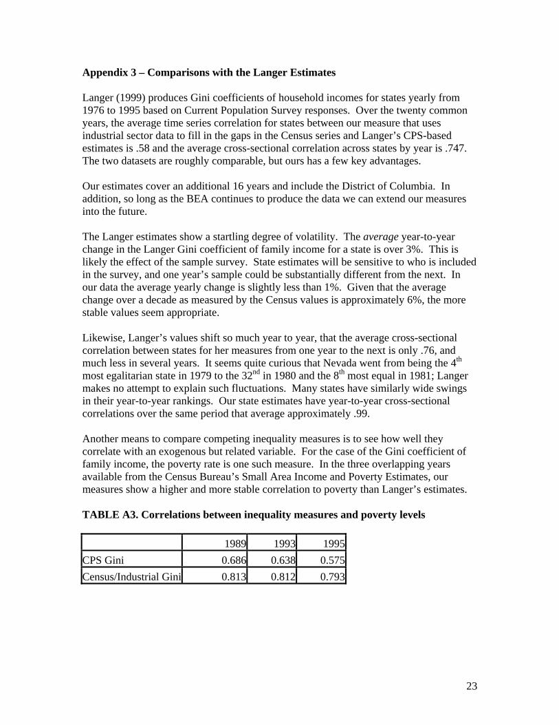
Appendix 3 – Comparisons with the Langer Estimates Langer (1999) produces Gini coefficients of household incomes for states yearly from 1976 to 1995 based on Current Population Survey responses. Over the twenty common years, the average time series correlation for states between our measure that uses industrial sector data to fill in the gaps in the Census series and Langer’s CPS-based estimates is .58 and the average cross-sectional correlation across states by year is .747. The two datasets are roughly comparable, but ours has a few key advantages. Our estimates cover an additional 16 years and include the District of Columbia. In addition, so long as the BEA continues to produce the data we can extend our measures into the future. The Langer estimates show a startling degree of volatility. The average year-to-year change in the Langer Gini coefficient of family income for a state is over 3%. This is likely the effect of the sample survey. State estimates will be sensitive to who is included in the survey, and one year’s sample could be substantially different from the next. In our data the average yearly change is slightly less than 1%. Given that the average change over a decade as measured by the Census values is approximately 6%, the more stable values seem appropriate. Likewise, Langer’s values shift so much year to year, that the average cross-sectional correlation between states for her measures from one year to the next is only .76, and much less in several years. It seems quite curious that Nevada went from being the 4th most egalitarian state in 1979 to the 32nd in 1980 and the 8th most equal in 1981; Langer makes no attempt to explain such fluctuations. Many states have similarly wide swings in their year-to-year rankings. Our state estimates have year-to-year cross-sectional correlations over the same period that average approximately .99. Another means to compare competing inequality measures is to see how well they correlate with an exogenous but related variable. For the case of the Gini coefficient of family income, the poverty rate is one such measure. In the three overlapping years available from the Census Bureau’s Small Area Income and Poverty Estimates, our measures show a higher and more stable correlation to poverty than Langer’s estimates. TABLE A3. Correlations between inequality measures and poverty levels 1989 1993 1995CPS Gini 0.686 0.638 0.575Census/Industrial Gini 0.813 0.812 0.793

24

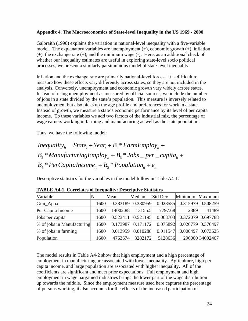
Appendix 4. The Macroeconomics of State-level Inequality in the US 1969 - 2000 Galbraith (1998) explains the variation in national-level inequality with a five-variable model. The explanatory variables are unemployment (+), economic growth (+), inflation (+), the exchange rate (+), and the minimum wage (-). Here, as an additional check of whether our inequality estimates are useful in exploring state-level socio political processes, we present a similarly parsimonious model of state-level inequality. Inflation and the exchange rate are primarily national-level forces. It is difficult to measure how these effects vary differently across states, so they are not included in the analysis. Conversely, unemployment and economic growth vary widely across states. Instead of using unemployment as measured by official sources, we include the number of jobs in a state divided by the state’s population. This measure is inversely related to unemployment but also picks up the age profile and preferences for work in a state. Instead of growth, we measure a state’s economic performance by its level of per capita income. To these variables we add two factors of the industrial mix, the percentage of wage earners working in farming and manufacturing as well as the state population. Thus, we have the following model:

1

2 3

4 5

** * _ _* *

it i t it

it it

it it it

Inequality State Year B FarmEmployB ManufacturingEmploy B Jobs per capitaB PerCapitaIncome B Population e

= + + ++ +

+ +

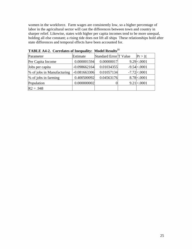
Descriptive statistics for the variables in the model follow in Table A4-1: TABLE A4-1. Correlates of Inequality: Descriptive Statistics Variable N Mean Median Std Dev Minimum MaximumGini_Appx 1600 0.383189 0.380959 0.028585 0.315979 0.508259Per Capita Income 1600 14002.88 13155.5 7797.68 2389 41489Jobs per capita 1600 0.523411 0.521195 0.063703 0.372079 0.697788% of jobs in Manufacturing 1600 0.173987 0.171172 0.075892 0.026779 0.376497% of jobs in farming 1600 0.013959 0.010288 0.011547 0.000497 0.073625Population 1600 4763674 3282172 5128636 296000 34002467 The model results in Table A4-2 show that high employment and a high percentage of employment in manufacturing are associated with lower inequality. Agriculture, high per capita income, and large population are associated with higher inequality. All of the coefficients are significant and meet prior expectations. Full employment and high employment in wage bargained industries brings the lower part of the wage distribution up towards the middle. Since the employment measure used here captures the percentage of persons working, it also accounts for the effects of the increased participation of

25

women in the workforce. Farm wages are consistently low, so a higher percentage of labor in the agricultural sector will cast the differences between town and country in sharper relief. Likewise, states with higher per capita incomes tend to be more unequal, holding all else constant; a rising tide does not lift all ships These relationships hold after state differences and temporal effects have been accounted for. TABLE A4-2. Correlates of Inequality: Model Results21 Parameter Estimate Standard Error T Value Pr > |t| Per Capita Income 0.000001594 0.00000017 9.29 <.0001 Jobs per capita -0.098662164 0.01034355 -9.54 <.0001 % of jobs in Manufacturing -0.081663306 0.01057134 -7.72 <.0001 % of jobs in farming 0.400500092 0.04563176 8.78 <.0001 Population 0.000000002 0 9.21 <.0001 R2 = .948

26

References Bernard, Andrew and J. Bradford Jensen (1998), “Understanding Increasing And Decreasing Wage Inequality,” National Bureau of Economic Research Working Paper 6571, Online, Available: http://www.nber.org/papers/w6571. Bernstein, J., H. Boushey, E. McNichol, and R. Zahradnik (2002), Pulling Apart: A State-by-State Analysis of Income Trends, Report from the Center on Budget and Policy Priorities and the Economic Policy Institute, April 2002. Bureau of Economic Analysis (1998), State Personal Income, 1927-1997, Online, Available: http://www.bea.doc.gov/bea/regional/articles/spi2997/. Bureau of Economic Analysis (2005), Regional Economic Accounts: Annual State Personal Income, Online, Available: http://www.bea.doc.gov/bea/regional/spi/. Bureau of Labor Statistics (2003), BLS Handbook of Methods, Online, Available: http://www.bls.gov/opub/hom/homch5_a.htm. Conceição, Pedro, James K. Galbraith, and Peter Bradford (2000); “The Theil Index in Sequences of Nested and Hierarchic Grouping Structures: Implications for the Measurement of Inequality through Time, with Data Aggregated at Different Levels of Industrial Classification,” Eastern Economic Journal, Volume 27, Pages 61 – 74. Ferguson, T. (2005), “Holy Owned Subsidiary: Globalization, Religion, and Politics in the 2004 Election” forthcoming in A Defining Election: The Presidential Race of 2004 edited by William Crotty, Armonk: M.E. Sharpe, Inc, 187-210. A longer version is available at http://utip.gov.utexas.edu/papers/utip_32.pdf. Galbraith, James K (1998), Created Unequal, The Free Press, New York. Galbraith, James K. (2004), “The voters Democrats can’t reach,” Online, Available: http://archive.salon.com/opinion/feature/2004/09/13/polarized_country/index_np.html. Galbraith, James K. and Enrique Garcilazo (2004), “Unemployment Inequality and the Policy of Europe: 1984-2000,” UTIP Working Paper No. 25, Online, Available: http://utip.gov.utexas.edu/papers/utip_25rv3.pdf. Galbraith, James K. and Travis Hale (2005), “Within-state Income Inequality and the Presidential Vote 1992 – 2004: A First Look at the Evidence,” UTIP Working Paper No. 29, Online, Available: http://utip.gov.utexas.edu/papers/utip_29.pdf. Galbraith, James K. and Hyunsub Kum (2004), “Estimating the Inequality of Household Incomes: A Statistical Approach to the Creation of a Dense and Consistent Global Data Set,” UTIP Working Paper No. 22, Online, Available: http://utip.gov.utexas.edu/papers/utip_22rv5.pdf.

27

Langer, Laura (1999), “Measuring Income Distribution across Space and Time in the American States,” Social Science Quarterly, Volume 80, Number 1, March, 55-67. Leip, D. (2005), Dave Leip's Atlas of U.S. Presidential Elections, Online, Available: http://uselectionatlas.org/USPRESIDENT/. U.S. Census Bureau (2005), “Table S4. Gini Ratios by State: 1969, 1979, 1989, 1999,” Online, Available: http://www.census.gov/hhes/income/histinc/state/state4.html. U.S. Census Bureau (2004), Table H-4. Gini Ratios for Households, by Race and Hispanic Origin of Householder: 1967 to 2003,” Online, Available: http://www.census.gov/hhes/income/histinc/h04.html.

28

Notes 1 Bernard and Jensen (1998) go even further, “Any theory of the rise in income inequality in the U.S. as a whole should also be capable of explaining the wide variety of outcomes across individual states.” 2 Other work from the University of Texas Inequality Project focuses on techniques to improve Gini coefficient estimates and the measurement of inequality at the subnational level. An example of using alternative techniques to improve Gini estimates can be found in Galbraith and Kum (2004). Galbraith and Garcilazo (2004) focuses on sub-national inequality in Europe. 3 Langer (1999); Bernard and Jensen (1998); Bernstein, Boushey, McNichol, and Zahradnik (2002). 4 The Gini coefficient of inequality is based on the Lorenz curve and compares the actual distribution of a resource – such as income – with a hypothetical distribution of perfect equality. Values of the Gini coefficient range from zero (perfect equality) to one (total inequality, where one person holds all of the resource). For additional information on the Gini coefficient, see Langer (1999). 5According to the BLS (2005), “The ES-202 program is a comprehensive and accurate source of employment and wage data, by industry, at the national, State, and county levels. It provides a virtual census of nonagricultural employees and their wages. In addition, about 47 percent of all workers in agricultural industries are covered.” Additional information on agricultural employees, sole proprietors, and other special categories of workers comes from “U.S. Department of Labor; the social insurance programs of the Health Care Financing Administration, U.S. Department of Health and Human Services, and the Social Security Administration; the Federal income tax program of the Internal Revenue Service, U.S. Department of the Treasury; the veterans benefit programs of the U.S. Department of Veterans Affairs; and the military payroll systems of the U.S. Department of Defense.” (BEA 1998) 6 The raw data can be download quite easily from the BEA’s website, www.bea.gov, through the Regional: State and Local Personal Income portal. 7 For a technical discussion of Theil’s T statistic, see Conceição, Galbraith, and Bradford (2000). 8 To get the best estimate of Theil’s T statistic using the available information, we need a group structure that is mutually exclusive and as completely exhaustive as possible. This requires a reorganization of the underlying data, such that we can always use the narrowest group levels, not the more aggregated categories. We prefer disaggregated categories such as Coal Mining or Motor Vehicles and Equipment Manufacturing to catch-all groups like Mining or Durable Goods Manufacturing. In some instances, values for the narrowest categories are suppressed or unreported. Thus, to cover all of the employment and wage values at the lowest possible levels, it is necessary to add in some “hidden” groups. For example, within Mining there are four subcategories: Metal, Coal, Oil and gas, and Nonmetallic minerals except fuels. If a state reports on employment and wages for Mining in the aggregate and Metal and Coal extraction individually, but the sum of the Metal and Coal extraction employment does not equal Mining in the aggregate, this indicates that there was some Oil and gas or Nonmetallic minerals except fuels activity, but reporting these values would reveal sensitive or unrevealed information. In this case, adding a group called “Hidden Mining” would allow us to continue to use the lowest level of aggregation without having any overlap across categories. Once these hidden values have been added, where appropriate, we can calculate the inter-industrial value of Theil’s T in every year for each state. 9 The BEA actually produces data series on incomes as well as wages. Unfortunately, this data does not distinguish between proprietors and employees at a detailed level. The income definitions for these two groups differs, making it difficult to interpret results of the inequality analysis. 10 We use the Census estimates of the family Gini to anchor the year-to-year estimates, rather than the household measure, a decision solely driven by data considerations. There are four values for the family income Gini coefficient in each state, but only three for the household measure. The cross-sectional

29

correlations between family and household inequality measures across states are very high – between .91 and .97 for each year. Since the two types of Gini coefficients contain basically the same information, we use the family measure to give the state regressions an additional degree of freedom.

11 The shift in industrial standards from SIC (1969-2000) to NAICS (2001-forward) creates a challenge in maintaining consistency in the inequality measures. While the technique remains the same, the new group structure results in some significant discontinuities in many of the state series – the average difference in within-state inequality measures with NAICS in 2001 and 2000 under SIC is over 11%, approximately twice as high as any of the year to year changes from 1969 to 2000. Thankfully, we do have data for both 2000 and 2001 for consistent SIC categories over 15 groups for each state. Values of Theil’s T statistic at this more aggregated level correlate highly with values with the more disaggregated measures both cross-sectionally and over time from 1969 to 2000. To bridge the gap from 2000 to 2001, we impute a value for the within-state Theil’s T for pay inequality 2001 by multiplying the percentage change in the aggregated measure from 2000 to 2001 by the disaggregated measure in 2000. Then we calculate a scaling factor by dividing the NAICS Theil value in 2001 with the imputed SIC Theil value for 2001. Multiplying the NAICS Theil values for 2002 – 2004 by the scaling factor results in a continuous time series. For the national-level time series, we use the difference in the CPS Gini coefficient from 2000 to 2001 to generate the scaling factor. 12 We use 2000 as the cutoff because this is when the industrial classification standard changes. If instead of using national level data to construct the Theil estimates, we use all of the state-sector data points, the correlation coefficient rises to .963. With smaller groups, we get more precise estimates. On the other hand, this significant increase in the number of groups only slightly increases the correlation, which indicates that fairly good estimates can be made with a relatively small number of groups. 13 Indeed, direct comparability between units of different size is the fundamental strength of the Gini coefficient and the best reason for transforming the Theil-based values of pay inequality into Gini coefficient approximations of income inequality. 14 The scale for Figures 1 and 2 do NOT include zero, so that year-to-year variations are easier to identify. 15 The BEA defines the following regions: New England – Connecticut, Maine, Massachusetts, New Hampshire, Rhode Island, Vermont Metro Atlantic – Delaware, Washington D.C., Maryland, New Jersey, New York, Pennsylvania Midwest – Illinois, Indiana, Michigan, Ohio, Wisconsin Great Plains – Iowa, Kansas, Minnesota, Missouri, Nebraska, North Dakota, South Dakota Southeast – Alabama, Arkansas, Florida, Georgia, Kentucky, Louisiana, Mississippi, North Carolina, South Carolina, Tennessee, Virginia, West Virginia Southwest – Arizona, New Mexico, Oklahoma, Texas Rocky Mountain – Colorado, Idaho, Montana, Utah, Wyoming Far West – Alaska, California, Hawaii, Nevada, Oregon, Washington 16 The percentage of a state’s population living in non-metropolitan counties and state per capita income are taken from the BEA online database (2005). Race data for 2000 are Census Bureau estimates. The 1992 and 1996 values are linear combinations of the 1990 and 2000 Census estimates. 2004 race data come from the Census Bureau’s American Community Survey. Voting outcome and turnout data come from Dave Leip's Atlas of U.S. Presidential Elections (2005). 17 Because of its particularly unusual characteristics, Washington D.C. is not included in the analysis. When included, the inequality variable becomes more significant in each analysis and maintains the same direction

18 With the exception of Rhode Island (+), the state fixed effects are insignificant.

30

19 We thank Andrew Gelman for pointing out an error in our previous effort to interpret this result. 20 It may be, for instance, that low income voters in high-income places feel poorer (as, relative to the cost of living, they are), and are correspondingly more likely to vote Democratic. Or it may be that those (relatively few) high income voters who lean Democratic also tend to cluster in cities, where lower-income voters are also to be found. These suppositions cannot be tested directly with our data. 21 The state and year dummy variables are suppressed.