Embed Size (px)
Citation preview
State Estimation Techniques
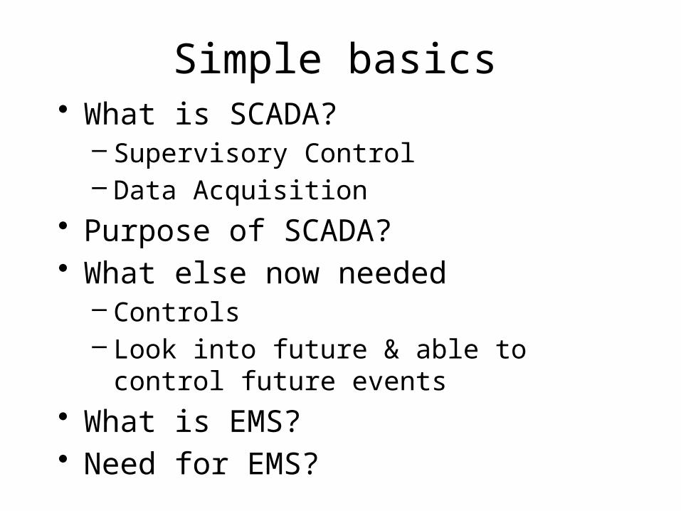
Simple basics• What is SCADA?
– Supervisory Control– Data Acquisition
• Purpose of SCADA?• What else now needed
– Controls – Look into future & able to control future events
• What is EMS?• Need for EMS?
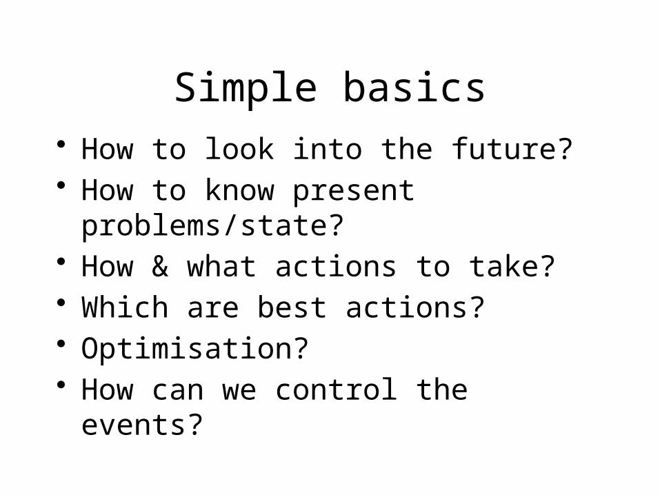
Simple basics• How to look into the future?• How to know present problems/state?• How & what actions to take?• Which are best actions?• Optimisation?• How can we control the events?
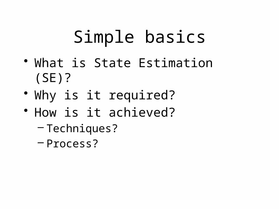
Simple basics• What is State Estimation (SE)?• Why is it required?• How is it achieved?
– Techniques?– Process?
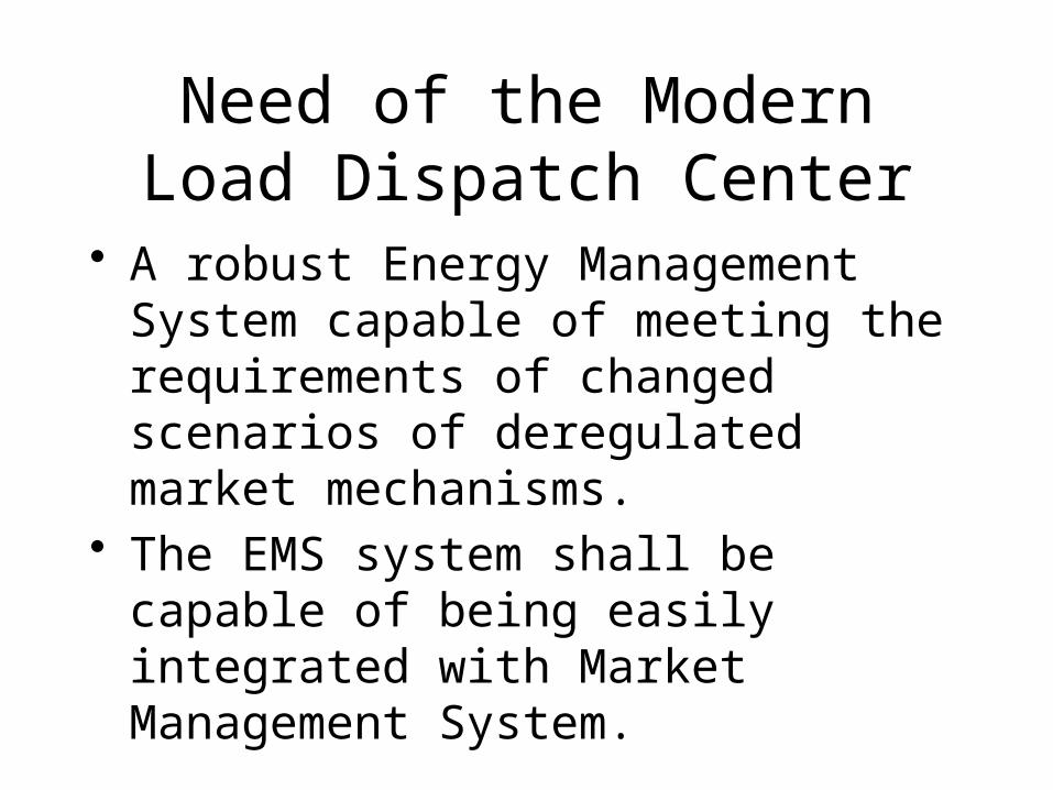
Need of the Modern Load Dispatch Center
• A robust Energy Management System capable of meeting the requirements of changed scenarios of deregulated market mechanisms.
• The EMS system shall be capable of being easily integrated with Market Management System.
6
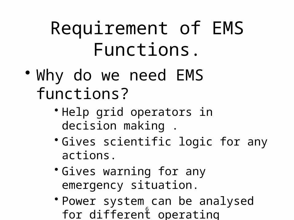
Requirement of EMS Functions.
• Why do we need EMS functions?• Help grid operators in decision making .• Gives scientific logic for any actions.• Gives warning for any emergency situation.• Power system can be analysed for different
operating conditions.• To get a base case for further Analysis• ….
EMS functions objective
• Power system monitoring
• Power system control
• Power system economics
• Security assessment
EMS Functions : Classification Based on Function
1. State Estimation
2. Power Flow Analysis
3. Contingency Analysis
4. Security enhancement
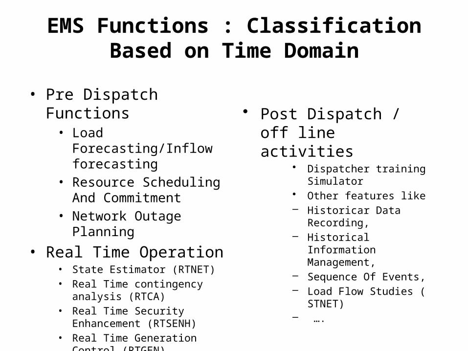
EMS Functions : Classification Based on Time Domain
• Pre Dispatch Functions• Load Forecasting/Inflow
forecasting• Resource Scheduling And
Commitment• Network Outage Planning
• Real Time Operation• State Estimator (RTNET)• Real Time contingency analysis
(RTCA)• Real Time Security Enhancement
(RTSENH)• Real Time Generation Control
(RTGEN)• Voltage Var Dispatch
• Post Dispatch / off line activities
• Dispatcher training Simulator
• Other features like– Historicar Data Recording,– Historical Information
Management,– Sequence Of Events,– Load Flow Studies
( STNET)– ….

2-10
SE Problem Development• What’s A State?
– The complete “solution” of the power system is known if all voltages and angles are identified at each bus. These quantities are the “state variables” of the system.
– Why Estimate?– Meters aren’t perfect.– Meters aren’t everywhere.– Very few phase measurements?– SE suppresses bad measurements and uses the
measurement set to the fullest extent.
Few Analogies given by F. Schweppe• Life blood of control system :
– clean pure data defining system state status (voltage, network configuration)
• Nourishment for this life blood: – from measurements gathered from around the system (data
acquisition)
• State Estimator: like a digestive system– removes impurities from the measurements– converts them into a form which brain (man/computer) of
central control centre can use to make “action” decisions on system economy, quality and security
EMS Functions
• Out of the all EMS functions State Estimator is the
first and most important function.
• All other EMS functions will work only when the
State Estimator is running well.
• State Estimator gives the base case for further
analysis.
State Estimation• State Estimation is the process of assigning a value to an unknown system
state variable based on measurements from that system according to some
criteria.
• The process involves imperfect measurements that are redundant and the
process of estimating the system states is based on a statistical criterion
that estimates the true value of the state variables to minimize or maximize
the selected criterion.
• Most Commonly used criterion for State Estimator in Power System is the
Weighted Least Square Criteria.
State Estimation• It originated in the aerospace industry where the basic problem have
involved the location of an aerospace vechicle (i.e. missile , airplane, or
space vechicle) and the estimation of its trajectory given redundant and
imperfect measurements of its position and velocity vector.
• In many applications, these measurements are based on optical
observations and/or radar signals that may be contaminated with noise and
may contain system measurement errors.
• The state estimators came to be of interest to power engineers in1960s.
Since then , state estimators have been installed on a regular basis in a new
energy control centers and have proved quite useful.
State Estimation• In the Power System, The State Variables are the voltage Magnitudes and
Relative Phase Angles at the System Nodes.
• The inputs to an estimator are imperfect power system measurements of
voltage magnitude and power, VAR, or ampere flow quantities.
• The Estimator is designed to produce the “best estimate” of the system
voltage and phase angles, recognizing that there are errors in the measured
quantities and that they may be redundant measurements.
2-16
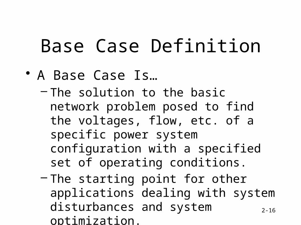
Base Case Definition
• A Base Case Is…– The solution to the basic network problem
posed to find the voltages, flow, etc. of a specific power system configuration with a specified set of operating conditions.
– The starting point for other applications dealing with system disturbances and system optimization.
Basics of state estimation
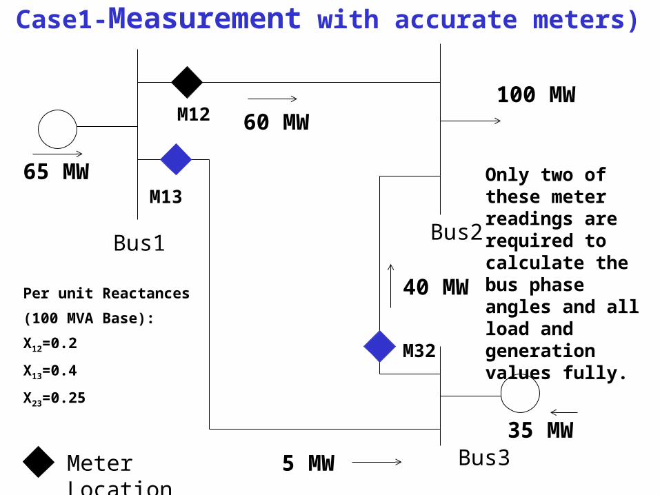
Bus1 Bus2
Bus3
60 MW
40 MW
65 MW
100 MW
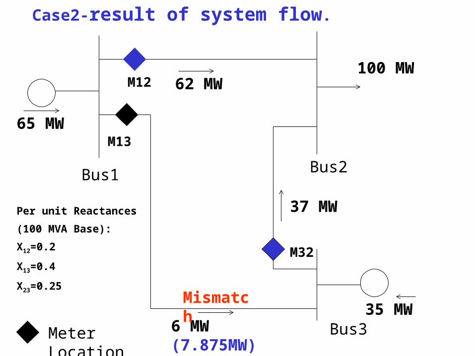
Per unit Reactances
(100 MVA Base):
X12=0.2
X13=0.4
X23=0.25
M12
M13
M32
5 MWMeter Location
35 MW
Case1-Measurement with accurate meters)
Only two of these meter readings are required to calculate the bus phase angles and all load and generation values fully.
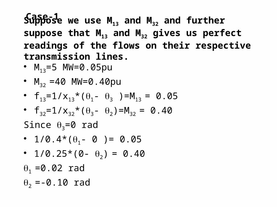
Suppose we use M13 and M32 and further suppose that M13 and M32 gives us perfect readings of the flows on their respective transmission lines.
• M13=5 MW=0.05pu
• M32 =40 MW=0.40pu
• f13=1/x13*(1- 3 )=M13 = 0.05
• f32=1/x32*(3- 2)=M32 = 0.40
Since 3=0 rad
• 1/0.4*(1- 0 )= 0.05
• 1/0.25*(0- 2) = 0.40
1 =0.02 rad
2 =-0.10 rad
Case-1
Bus1 Bus2
Bus3
62 MW
37 MW
65 MW
100 MW
Per unit Reactances
(100 MVA Base):
X12=0.2
X13=0.4
X23=0.25
M12
M13
M32
6 MW (7.875MW)Meter Location
35 MW
Case2-result of system flow.
Mismatch
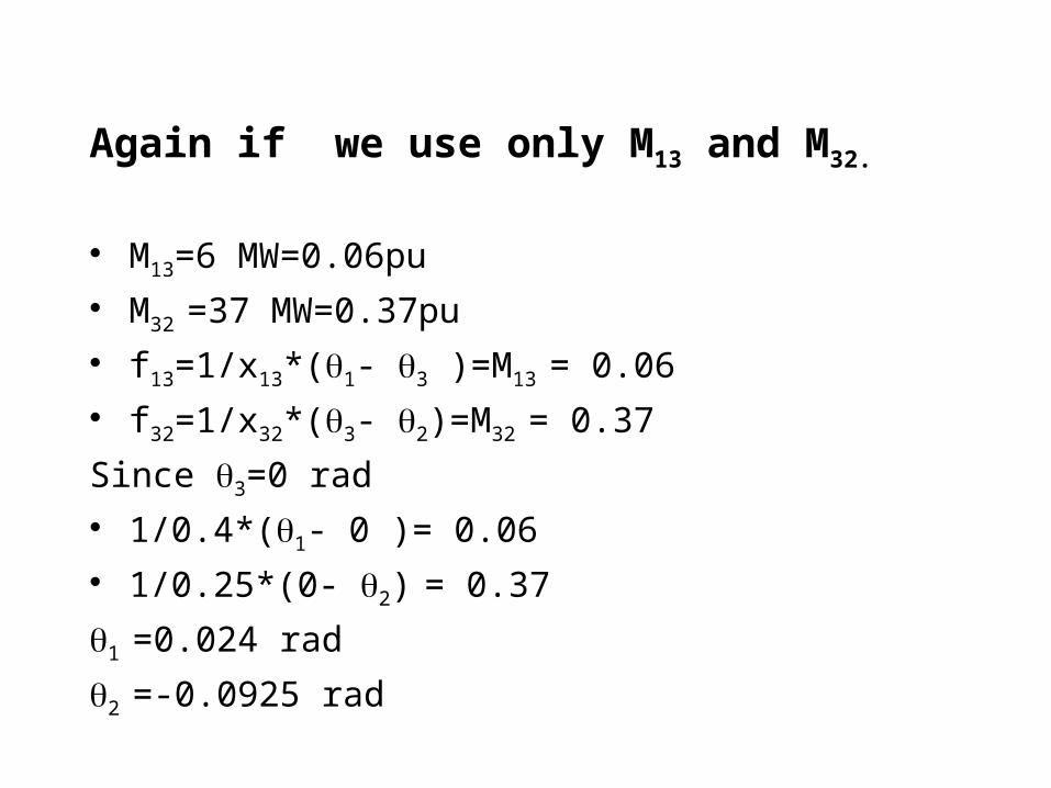
Again if we use only M13 and M32.
• M13=6 MW=0.06pu
• M32 =37 MW=0.37pu
• f13=1/x13*(1- 3 )=M13 = 0.06
• f32=1/x32*(3- 2)=M32 = 0.37
Since 3=0 rad
• 1/0.4*(1- 0 )= 0.06
• 1/0.25*(0- 2) = 0.37
1 =0.024 rad
2 =-0.0925 rad
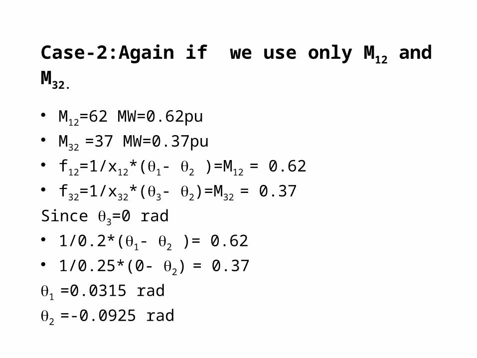
Case-2:Again if we use only M12 and M32.
• M12=62 MW=0.62pu
• M32 =37 MW=0.37pu
• f12=1/x12*(1- 2 )=M12 = 0.62
• f32=1/x32*(3- 2)=M32 = 0.37
Since 3=0 rad
• 1/0.2*(1- 2 )= 0.62
• 1/0.25*(0- 2) = 0.37
1 =0.0315 rad
2 =-0.0925 rad
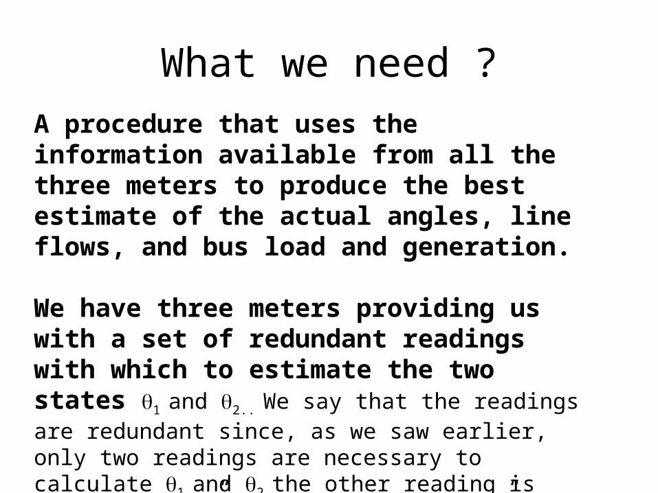
What we need ?
A procedure that uses the information available from all the three meters to produce the best estimate of the actual angles, line flows, and bus load and generation.
We have three meters providing us with a set of redundant readings with which to estimate the two states 1 and 2.. We say that the readings are redundant since, as we saw earlier, only two readings are necessary to calculate 1 and 2 the other reading is always “extra”. However, the “extra” reading does carry useful information and ought not to be discarded summarily.
2-24
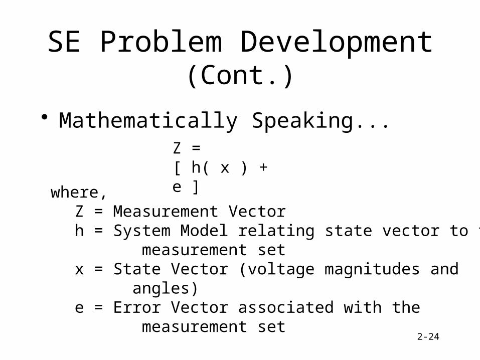
SE Problem Development (Cont.)
• Mathematically Speaking...Z = [ h( x ) + e ]
where,Z = Measurement Vectorh = System Model relating state vector to the measurement setx = State Vector (voltage magnitudes and angles)e = Error Vector associated with the measurement set

2-25
SE Problem Development (Cont.)
• Linearizing…
• Classical Approach -> Weighted Least Squares…
Z = H x + e
(This looks like a load flow equation )
Minimize: J(x) = [z - h(x)] t. W. [z - h(x)] where,
J = Weighted least squares matrixW = Error covariance matrix
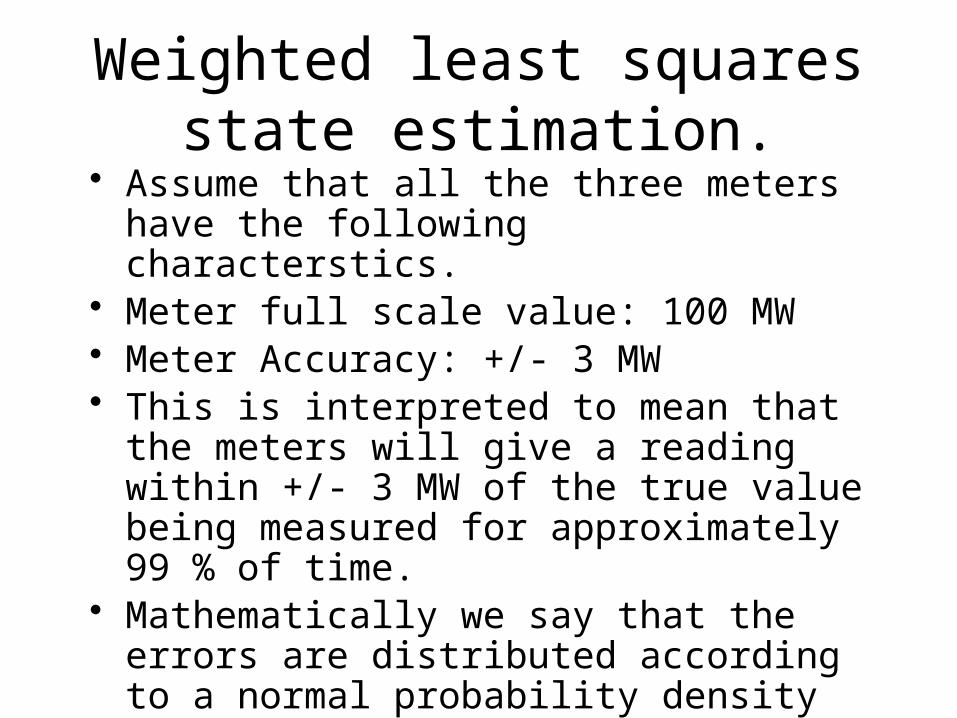
Weighted least squares state estimation.
• Assume that all the three meters have the following characterstics.
• Meter full scale value: 100 MW• Meter Accuracy: +/- 3 MW• This is interpreted to mean that the meters will
give a reading within +/- 3 MW of the true value being measured for approximately 99 % of time.
• Mathematically we say that the errors are distributed according to a normal probability density function with a standard deviation ,,
• I.e. +/- 3 MW corresponds to a metering standard deviation of , =1 MW=0.01 pu.

• X est =[ [H]T[R-1][H] ]-1 X [H]T[R-1]Zmeas
• [H]= an Nm by Ns matrix containing the coefficients of the linear functions fi(x)
• [R] = 1 2
2 2
..
Nm 2
• [Z meas]= Z 1meas
Z 2meas
.
.
Z Nmmeas
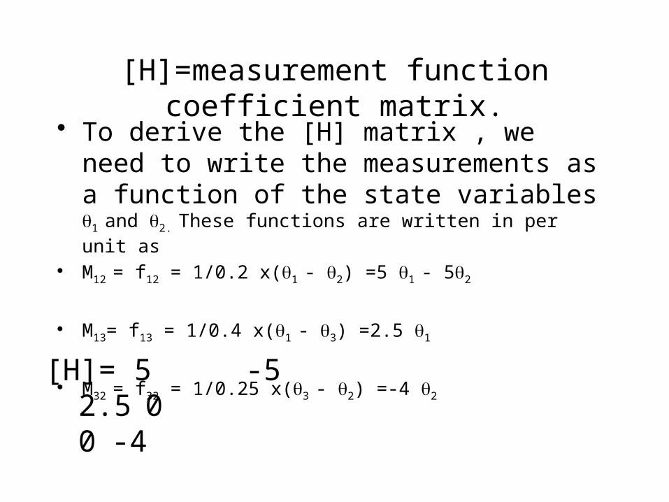
[H]=measurement function coefficient matrix.• To derive the [H] matrix , we need to write the
measurements as a function of the state variables 1
and 2. These functions are written in per unit as
• M12 = f12 = 1/0.2 x(1 - 2) =5 1 - 52
• M13= f13 = 1/0.4 x(1 - 3) =2.5 1
• M32 = f32 = 1/0.25 x(3 - 2) =-4 2
[H]= 5 -52.5 00 -4
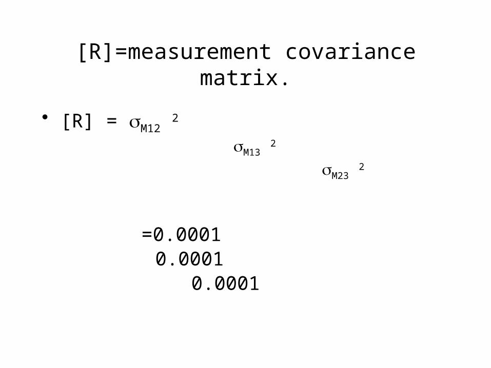
[R]=measurement covariance matrix.
• [R] = M12 2
M13 2
M23 2
=0.0001 0.0001
0.0001
2-30
SE Functionality
• So What’s It Do?– Identifies observability of the power system.– Minimize deviations of measured vs estimated
values.– Status and Parameter estimation.– Detect and identify bad telemetry.– Solve unobservable system subject to
observable solution.– Observe inequality constraints (option).
2-31
SE Measurement Types• What Measurements Can Be Used?
– Bus voltage magnitudes.– Real, reactive and ampere injections.– Real, reactive and ampere branch flows.– Bus voltage magnitude and angle differences.– Transformer tap/phase settings.– Sums of real and reactive power flows.– Real and reactive zone interchanges.– Unpaired measurements ok
2-32
State Estimation Process
• Two Pass Algorithm– First pass… observable network.– Second pass… total network (subject to first
pass solution).– High confidence to actual measurements.– Lower confidence to schedule values.– Option to terminate after first pass.
2-33
Observability Analysis
• Bus Observability– A bus is observable if enough information is
available to determine it’s voltage magnitude and angle.
– Observable area can be specified (“Region of Interest”).• Bus or station basis
2-34
Bad Data Suppression
• Bad Data Detection– Mulit-level process.– “Bad data pockets” identified.– Zoom in on “bad data pocket’ for rigorous
topological analysis.– Status estimation in the event of topological
errors.
2-35
Final Measurement Statuses• Used… The measurement was found to be “good” and
was used in determining the final SE solution.
• Not Used… Not enough information was available to use this information in the SE solution.
• Suppressed… The measurement was initially used, but found to be inconsistent (or “bad”).
• Smeared… At some point in the solution process, the measurement was removed. Later it was determined that the measurement was “smeared” by another bad measurement.
2-36
Solution Algorithms
• Objective… Weighted Least Squares:
• Choice of Givens Rotation or Hybrid Solution Methods
Minimize: J(x) = .5 [Z - h(x)] t R -1 [Z - h(x)]where,
J = Weighted least squares matrixR = Error covariance matrix
2-37
Solution Algorithms (Cont.)
• Given’s Rotation (Orthogonalization)– Least tendency for numerical ill-conditioning. – Uses orthogonal transformation methods to
minimize the classical least squares equation.– Higher computational effort.– Stable and reliable.
2-38
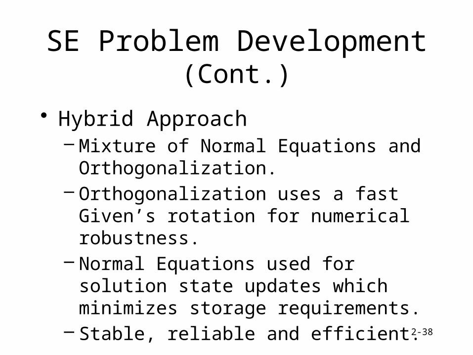
SE Problem Development (Cont.)
• Hybrid Approach– Mixture of Normal Equations and
Orthogonalization.– Orthogonalization uses a fast Given’s rotation
for numerical robustness.– Normal Equations used for solution state
updates which minimizes storage requirements.– Stable, reliable and efficient.
2-39
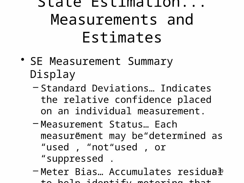
State Estimation...Measurements and Estimates
• SE Measurement Summary Display– Standard Deviations… Indicates the relative
confidence placed on an individual measurement.
– Measurement Status… Each measurement may be determined as “used”, “not used”, or “suppressed”.
– Meter Bias… Accumulates residual to help identify metering that is consistently poor. The bias value should “hover” about zero.
2-40
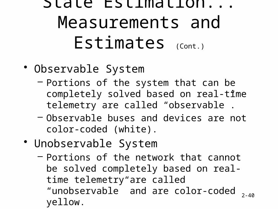
State Estimation...Measurements and Estimates (Cont.)
• Observable System– Portions of the system that can be completely solved
based on real-time telemetry are called “observable”.– Observable buses and devices are not color-coded
(white).
• Unobservable System– Portions of the network that cannot be solved
completely based on real-time telemetry are called “unobservable” and are color-coded yellow.
2-41
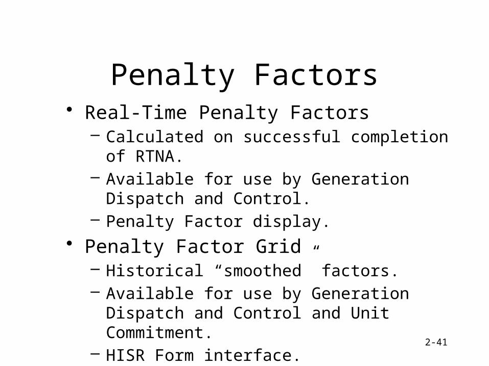
Penalty Factors• Real-Time Penalty Factors
– Calculated on successful completion of RTNA.– Available for use by Generation Dispatch and Control.– Penalty Factor display.
• Penalty Factor Grid– Historical “smoothed” factors.– Available for use by Generation Dispatch and Control
and Unit Commitment.– HISR Form interface.
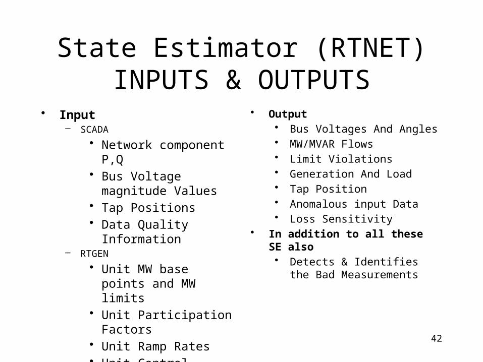
State Estimator (RTNET) INPUTS & OUTPUTS
• Input– SCADA
• Network component P,Q• Bus Voltage magnitude
Values• Tap Positions• Data Quality Information
– RTGEN
• Unit MW base points and MW limits
• Unit Participation Factors• Unit Ramp Rates• Unit Control Status and
on/off line status• Scheduled Area
Transactions
• Output• Bus Voltages And Angles• MW/MVAR Flows• Limit Violations• Generation And Load• Tap Position• Anomalous input Data• Loss Sensitivity
• In addition to all these SE also • Detects & Identifies the Bad
Measurements
42
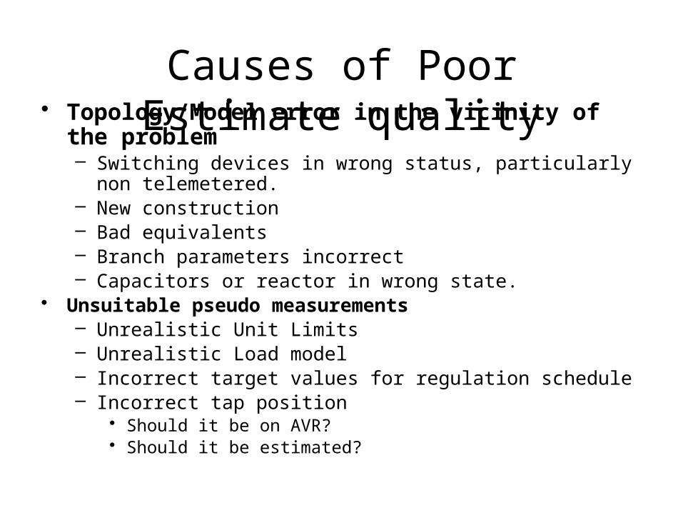
Causes of Poor Estimate quality• Topology/Model error in the vicinity of the problem– Switching devices in wrong status, particularly non telemetered.– New construction– Bad equivalents– Branch parameters incorrect– Capacitors or reactor in wrong state.
• Unsuitable pseudo measurements– Unrealistic Unit Limits– Unrealistic Load model– Incorrect target values for regulation schedule– Incorrect tap position
• Should it be on AVR?• Should it be estimated?
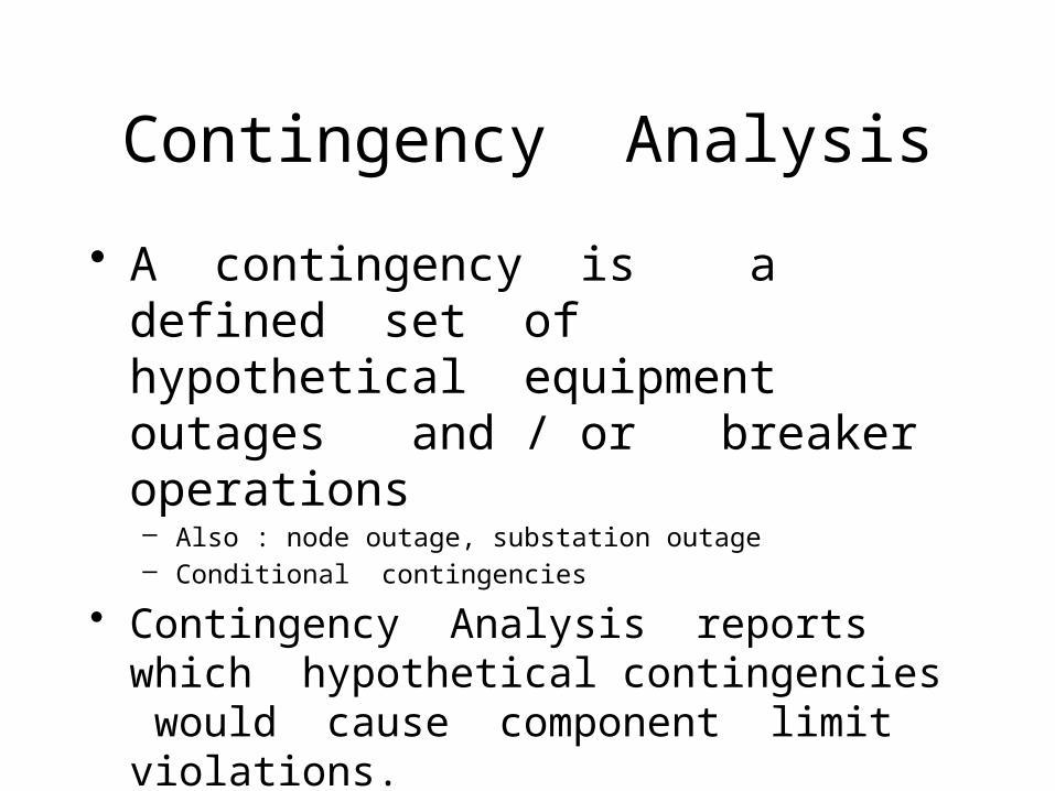
Contingency Analysis
• A contingency is a defined set of hypothetical equipment outages and / or breaker operations– Also : node outage, substation outage– Conditional contingencies
• Contingency Analysis reports which hypothetical contingencies would cause component limit violations.
45
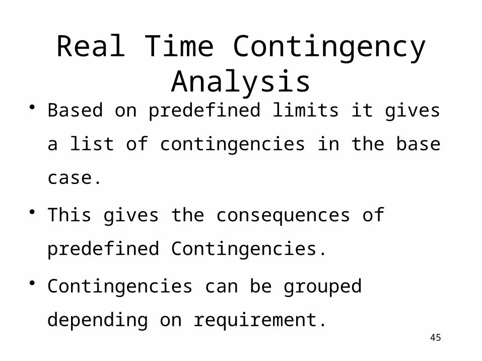
Real Time Contingency Analysis• Based on predefined limits it gives a list of
contingencies in the base case.
• This gives the consequences of predefined
Contingencies.
• Contingencies can be grouped depending on
requirement.
Requirement for Good CA results:
• A good Base Case based on the State
Estimator Output.
• Defined all the possible credible
contingencies.
• Correct limits for all power system
elements.