State Economic Performance and Effective Tax Ratesglobalbizresearch.org/economics/images/files/44668_ID_1132_JEIEFB... · Journal of Emerging Issues in Economics, Finance and Banking

Journal of Emerging Issues in Economics, Finance and Banking (JEIEFB)

An Online International Research Journal (ISSN: 2306-367X)

2017 Vol: 6 Issue: 2

2350 www.globalbizresearch.org

State Economic Performance and Effective Tax Rates

Pavel A. Yakovlev,

Dept. of Economics,

Duquesne University, Pittsburgh, USA.

Saurav Roychoudhury,

Dept. of Business,

Capital University, Columbus, USA.

E-mail: [email protected]

___________________________________________________________________________________

Abstract

The causal relationship between economic growth and taxation has been difficult to ascertain

empirically. Some of the common empirical challenges encountered in this line of research

include non-linearity and endogeneity of the relationship between economic growth and

taxation. This study controls for the non-linearity and endogeneity of tax effects in an attempt

to estimate a genuinely causal relationship between economic performance and taxation.

Using a longitudinal panel of American states, we estimate how the effective average tax rate

affects state economic growth and per capita income. We find that a higher effective average

tax rate reduces not only state economic growth but also real gross state product (GSP) per

capita.

___________________________________________________________________________

Key Words: prosperity, income, economic growth, taxation, endogeneity, non-linearity

JEL codes: H2, H3, O4





1. Introduction

The inquiry into the relationship between economic prosperity and taxation is probably as

old as the economics discipline itself (Smith, 1880). Despite no shortage of research on this

topic, the empirical consensus on the growth-taxation nexus remains elusive (Pjesky 2006,

Alm and Rogers 2011). In this paper, we conduct an empirical test of the economic

performance-taxation nexus using some of the best aggregate data available in the world: a

longitudinal panel of American States. In comparison to international data, which are often

fraught with reliability issues and other challenges, the U.S state-level data are usually more

accurate and rich. Furthermore, the existence of uniform national institutions and monetary

policy across American states lowers the unobserved heterogeneity bias and allows for a more

authoritative analysis of an already challenging topic. Our findings on the growth-tax

relationship at a sub-national level have implications for the other economies as well,

particularly those in the European Union.

In this paper, we estimate the impact of the effective average state tax rate on both real

gross state product (GSP) per capita and its growth rate. Looking at these two measures of

economic performance separately can enrich our understanding of taxation’s impact on

aggregate economic activity and help clarify some of the inconsistencies in previous findings.

In addition to that, we try to address two empirical challenges that have plagued this line of

research in the past: the endogeneity of tax rates (Grossman 1988, Karagianni et al. 2013) and

possible non-linearity in the relationship between economic performance and taxation

(Jaimovich and Rebelo 2012). After controlling for these issues, our analysis suggests that a

robust and quantitatively strong negative relationship exists between state economic growth

and effective average tax rate. However, the relationship between GSP per capita and the tax

rate appears to be non-linear. We explore whether outliers or endogenous tax policy might

account for this non-linearity.

2. Economic Performance and Taxation

Real gross domestic product (GDP) is the premier indicator of national economic

prosperity and the standard of living. Not surprisingly, the growth in real GDP per capita is

one of the most studied variables in the social sciences. A growing number of studies suggest

that higher taxes may reduce economic growth. 1 However, the empirical literature on

economic growth and taxation has produced somewhat paradoxical results (Tomljanovich,

2004). On the one hand, the empirical results on the growth-tax relationship appear to be

mixed, but there is a growing consensus that the tax-induced reductions in private investment

1 See, for example, Plaut and Pluta (1983), Benson and Johnson (1986), Canto and Webb (1987),

Vedder (1990, 2001), Berry and Kasermman (1993), Bahl and Sjoquist (1990), Hines (1996), Besci

(1996), Reed (2008), and Romer and Romer (2010), Yakovlev (2014).





spending and innovation hurt economic growth. For example, Widmalm (2001) studies the

effect of taxation on economic growth in 23 OECD countries and finds that higher income tax

progressivity lowers economic growth, corroborating earlier findings by Plosser (1992).

Johansson et al. (2008) find corporate income taxes to be most harmful to economic growth,

followed by personal income taxes, and consumption taxes, respectively. Finally, a seminal

paper by Romer and Romer (2010) demonstrates that exogenous increases in taxes lead to

strong contractions in investment and GDP.

The aforementioned ambiguity in empirical findings can be partially attributed to the

theoretical complexities. In the neoclassical growth model (Solow, 1956), saving and

investment is exogenous, which means that taxation does not influence the long-run growth

rate of the economy (Lee and Gordon 2005). Therefore, taxation may only have a temporary

impact on economic growth through its effect on some transitory level of income. The

neoclassical growth model predicts income convergence and views exogenous technological

progress as the primary source of the long-run economic growth, while the endogenous

growth model does not guarantee income convergence. In fact, the endogenous growth

models developed by Romer (1986, 1990) and Lucas (1988) suggest that taxation could

influence the endogenous saving and investment decisions, thereby affecting the long-run

growth rate. Arin et al. (2011) find that a rise in the marginal tax rate has a significant

negative impact on economic growth in Scandinavian countries, the United Kingdom, and the

United States. Jaimovich and Rebelo (2012) modify the endogenous growth model to show

that under entrepreneurial heterogeneity and mobility, tax rate increases have a small impact

on growth when tax rates are low or moderate, but when tax rates are high, further tax hikes

have a large negative impact on growth rates.

Several studies using state-level data from the United States show an adverse effect of

taxation on economic growth. Helms (1985) finds that state taxes have a significant negative

impact on state personal income. Helms also finds that tax-financed spending on health,

highways, and education has a positive impact on state personal income that helps to mitigate

the negative effect of taxation. This lends some support for Barro’s (1990) model of public

infrastructure spending where taxes that fund productive government spending can have a

positive effect on growth. Even after controlling for state government spending on health,

education, and highways, Mofidi and Stone (1990) find higher state taxes as a share of

income have a significant negative impact on the growth of manufacturing employment.

Poulson and Kaplan (2008) find that higher marginal tax rates have a significant negative

impact on state economic growth after controlling for tax regressivity, convergence, and

regional influences. Reed (2008) finds that a larger federal government sector and a higher

average tax rate (in levels and differences) is associated with lower state economic growth. In





a policy report, Laffer et al. (2012) point out that states without personal income taxes tend to

have higher growth in GDP, population, employment, and even tax revenues. Similarly,

Yakovlev (2014) finds that higher state taxes reduce the number of firms and state economic

growth.

The described findings on growth and taxation need to be treated with caution, however.

For example, Alm and Rogers (2011), find that the correlation between economic growth and

taxation is often statistically significant, but can be sensitive to the chosen regressors and time

periods. Similarly, Pjesky (2006) also find that results depend on the time period and the

choice of dependent variables. Gale and Samwick’s (2016) review of the relevant literature

suggests that not all tax changes will have the same impact on growth and that the net effect

of tax cuts will depend on the spending cuts as well.

Moreover, tax policy can be endogenous, further complicating the estimation of a causal

relationship between economic performance and taxation. Romer and Romer (2010) rightly

note that since changes in tax policy are often correlated with the other simultaneous

developments in the economy, it is often difficult to disentangle these effects from one

another. As a result, Romer and Romer (2010) attempt to separate the exogenous changes in

the U.S. federal tax policy from the endogenous ones and estimate the effects of the former on

economic growth. Their estimates reveal that exogenous changes in taxation have very large

effects on the U.S. real output. Namely, they calculate that a 1 percent increase in taxes

lowers real GDP by almost 3 percent.

We think that some of the differences in the empirical findings can be attributed to

potential non-linearity and likely endogeneity (i.e., reverse causality) in the relationship

between economic prosperity and taxation. In the following section, we address these two

issues while estimating the effect of taxation on both the level of state income per capita as

well as its growth rate.

3. Empirical Modeling

Typically, economists seek to examine the effect of the marginal tax rate on economic

growth because this tax measure tends to capture the disincentives to work and invest better

than the average tax rate, for example. One of the traditional approximations for the combined

marginal tax rate used in the previous literature (see Koester and Kormendi 1989, for

example) is obtained by estimating the following equation:

𝑇𝑎𝑥 𝑟𝑒𝑣𝑒𝑛𝑢𝑒 = 𝛼 + 𝛽(𝐺𝐷𝑃) + 휀, (1)

where α is the y-intercept, β serves as a linear approximation for the effective marginal tax

rate (β > 1 indicates a progressive tax system), and ε is the error term. This approach assumes

that the tax rate remains constant over time, which is not the case for the period examined in

this study. Another fundamental problem here is that state economic performance may factor





into the determination of the marginal tax rate (β), so the marginal tax rate is likely to be

endogenous. This implies that either good or poor economic performance may force

policymakers to change the marginal tax rate, obfuscating the empirical estimates of how

taxes impact economic growth (Romer and Romer 2010, Karagianni et al. 2013). Solving the

above equation for the marginal tax rate (β) demonstrates that the set tax rate depends on the

desired amount of tax revenue, GDP, and other factors that are captured by the error term (ε):

𝛽 =𝑇𝑎𝑥 𝑟𝑒𝑣𝑒𝑛𝑢𝑒

𝐺𝐷𝑃−

𝛼

𝐺𝐷𝑃−

𝜀

𝐺𝐷𝑃. (2)

Notice that tax revenue divided by GDP is essentially the average tax rate2. Solving the

above equation for the average tax rate shows that it is a function of the marginal tax rate,

GDP, and some other factors captured in the error term (ε):

𝑇𝑎𝑥 𝑟𝑒𝑣𝑒𝑛𝑢𝑒

𝐺𝐷𝑃= 𝛽 +

𝛼

𝐺𝐷𝑃+

𝜀

𝐺𝐷𝑃. (3)

Equation 3 suggests that the average tax rate is also endogenous.3 The likely endogeneity

of both the marginal and average tax rates requires going beyond the conventional OLS

regression to obtain more reliable estimates. One such popular method is the within or fixed-

effects estimator, which captures some unobserved factors that are correlated with the

regressors. While this estimator is quite good at correcting for the omitted variable bias that

gives rise to one source of the endogeneity problem, it does not address the other source of

endogeneity bias: the reverse causality stemming from economic performance to policy-

induced tax rate changes. Fortunately, this form of endogeneity can be addressed using the

instrumental variable (IV) method.

While both the marginal and average tax rates are likely to be endogenous, the effective

average tax rate has the advantage of being easily observed and calculated every year. In

contrast, when using marginal tax rates, researchers are often forced to use cross-section data

or fewer years for which marginal tax information is available, which is problematic. Also,

the existence of multiple taxes makes it difficult to combine all of the relevant marginal tax

rates into a single aggregate measure that can be used to analyze the impact of the overall tax

structure on GSP and its growth rate. Therefore, this study uses the effective average state tax

rate as a practical approximation of the overall state tax burden.4 The US state-level data is

chosen due to its reliability and availability of a rich set of control variables over relatively

2 This is the effective average tax rate: a ratio of taxes paid to total income. 3 Koester and Kormendi (1989) argue that the average tax rate is endogenous in income, which

complicates the estimation of the true relationship between economic growth and the average tax rate.

In an analysis of 63 countries, they find that neither marginal nor average tax rates have any effect on

economic growth, but they do find that higher marginal tax rates (assuming revenue neutrality) reduce

the level of economic activity. 4 The effective average tax rate is measured as state tax revenue divided by gross state product.





long periods of time. Furthermore, the presence of uniform economic and political institutions

in this sample helps to minimize unobserved heterogeneity bias. Missing observations for

some key control variables for Florida and the use of lagged variables reduce the available

sample to 49 states and over the 1977-2000 period. The dataset we end up using strikes a

balance between having too few control variables and observations. In Table 1, we show

variable definitions, summary statistics, and data sources used in this study.

Table 1. Variable Definitions and Summary Statistics

Variable Mean

(Std. Dev.)

Min.

(Max.) a Physical capital investment per capita ($’s) 156,784 (47,908) 85,150 (668,134)

a Farmland value per capita ($’s) 13,353 (11,789) 833 (73,442)

a Educational attainment (workforce’s average years of schooling) 12.26 (0.96) 9.31 (14.44)

a Average age of state population between 16 and 65 years old 37.26 (1.54) 30.46 (41.65)

b Gross state product (GSP) per capita ($’s) 31,672 (8,408) 16,346 (111,227)

b Growth in GSP per capita 0.03 (0.04) −0.29 (0.43)

b Federal civilian government workers as a share of all employed 0.013 (0.007) 0.005 (0.06)

c Average tax rate = tax revenue/GSP 0.05 (0.01) 0.01 (0.11)

c Working-age people (between 16 and 65) as a share of population 0.60 (0.03) 0.22 (0.85)

c Public infrastructure spending per capita ($’s) 351 (188) 121 (2,083)

c Natural resource value (millions of $’s per capita) 81.22 (77.44) 2.21 (923)

c Federal aid to states per capita ($’s) 902 (406) 103 (4,042)

c Population growth 0.01 (0.01) −0.03 (0.1)

c Population density (people per square mile) 139 (183) 0.45 (998)

Sources: (a) Obtained from Turner et al. (2007, 2011). (b) US Bureau of Economic Analysis. (c)

Statistical Abstracts, US Census Bureau. (d) Computed from the Book of States data. Notes: All

monetary variables are adjusted for inflation.

We first estimate the impact of the effective average tax rate on economic growth using

the conventional ordinary least squares (OLS) estimator with the state (ui) and year (vt) fixed

effects and Driscoll and Kraay (1998) standard errors:5

(𝐺𝑆𝑃 𝑔𝑟𝑜𝑤𝑡ℎ)𝑖𝑡 = 𝛼 + 𝛾 (𝐺𝑆𝑃

𝑐𝑎𝑝𝑖𝑡𝑎)

𝑖,𝑡 − 5+ 𝛽1(𝑡𝑎𝑥 𝑟𝑎𝑡𝑒)𝑖𝑡 + 𝑋𝑖𝑡𝛽𝑗 + 𝑢𝑖 + 𝑣𝑡 + 휀𝑖𝑡 (4)

The regression model in equation 4 follows the conventional Solow-type growth

specification (see, for example, Mankiw et al. 1992, Yakovlev 2007). It contains the

convergence factor (five-year lag of GSP per capita) that captures the tendency of richer

states to grow more slowly than poorer states. The model also contains a typical set of control

variables in Xit such as human and physical capital, public infrastructure investment,

demographic, fiscal, and other common determinants of economic growth (see Turner et al.

2007, 2011 for state data on some of the key determinants of economic growth).

5 Driscoll and Kraay (1998) standard errors are robust to the general forms of autocorrelation,

heteroskedasticity, and contemporaneous correlation, all of which were detected in the error term.





If the average tax rate is endogenous (i.e., depends on the level of economic activity), the

OLS model may produce a biased estimate of taxation’s impact on economic growth. To

address this issue, we also estimate the following model using the System General Method of

Moments (GMM) developed by Arellano and Bover (1995) and Blundell and Bond (1998):

∆(𝐺𝑆𝑃 𝑔𝑟𝑜𝑤𝑡ℎ)𝑖𝑡 = 𝛼 + 𝛿∆(𝐺𝑆𝑃 𝑔𝑟𝑜𝑤𝑡ℎ)𝑖,𝑡 − 1 + 𝛾∆ (𝐺𝑆𝑃


𝑖,𝑡 − 5

+𝛽1∆(𝑡𝑎𝑥 𝑟𝑎𝑡𝑒)𝑖𝑡 + ∆𝑋𝑖𝑡𝛽𝑗 + ∆𝑣𝑡 + ∆휀𝑖𝑡 (5)

The reason we use the Arellano–Bover/Blundell–Bond estimator because it is a marked

improved over the difference GMM estimators. Our method works best with one left-hand-

side variable that is dynamic, depending on its own past realizations, independent variables

that are not strictly exogenous, meaning they are correlated with past and possibly current

realizations of the error, fixed individual effects; and heteroskedasticity and autocorrelation

within states but not across them. The Arellano–Bover/Blundell–Bond estimator augments

Arellano–Bond by making an additional assumption that first differences of instrument

variables are uncorrelated with the fixed effects. This allows the introduction of more

instruments and can dramatically improve efficiency. It builds a system of two equations—the

original equation and the transformed one—and is known as system GMM. Our regression

model in equation 5 includes a one-year lag of the dependent variable in addition to the

variables mentioned before. The first-differencing procedure of our system GMM estimator

removes time-invariant, unobserved heterogeneity (i.e., state fixed effects and invariant

variables).6 The average tax rate and the lagged dependent variable are instrumented with

their lagged levels (t − 2 and deeper) and first differences (t − 1 and deeper). The use of valid

instruments can improve the odds of capturing a real causal relationship in the tax

coefficients.

6 The first-differencing procedure removes the constant, which is added back into the model during the

estimation process. The Sargan IV and Arellano-Bond autocorrelation tests shown in table 2 attest to

the validity of the chosen instruments and the absence of 2nd-order autocorrelation, respectively.





Figures 1 and 2: The Relationship between Real GSP and Its Growth versus Tax Rate

Before we delve into the description of our regression results, it might be worthwhile to

examine the possibility of a non-linear relationship between state economic prosperity and the

effective average tax rate visually. In Figure 1, we test for a non-parametric relationship

between economic growth and the effective average state tax rate using the locally weighted

regression estimated by a LOWESS7 smoother. In Figure 2, we perform the same analysis,

but now between the natural log of real GSP per capita and the effective average tax rate. In

Figure 1, there is a clear linear negative relationship between GSP growth rate and the

average tax rate. However, in Figure 2 the relationship appears to be non-linear or “J” shaped.

At first, income per capita seems to fall marginally as the tax rate rises, but after an inflection

point, both variables begins to rise. The marginally negative relationship at low tax rates does

not support Grossman’s (1988) argument that a positive relationship between GDP per capita

and taxes could be present if public goods are provided efficiently at relatively low tax rates.

The observed positive relationship between GSP and higher tax rates might be indicative of

either outliers or reverse causality, where richer states can afford to enact higher taxes to

pursue progressive objectives (Karagianni et al. 2013, Yakovlev 2014). In other words, this

non-linearity might be the result of the endogenous nature of tax policy.

7 LOWESS is an acronym for 'Locally weighted Scatter plot Smoother'. The smoothing process is

considered local because each smoothed value is determined by neighboring data points defined within

the span. A regression weight function is defined for the data points contained within the span.

-.1

-.05

0

.05

.1.1

5

Real G

SP

Gro

wth

0 .02 .04 .06 .08 .1

State Effective Average tax rate

Figure 1: Real GSP growth vs. Tax rate

9.5

10

10

.511

11

.5

Lo

g o

f G

SP

Pe

r C

apita

0 .02 .04 .06 .08 .1

State Effective Average Tax Rate

Figure 2: GSP per capita vs. Tax rate





Table 2: Determinants of Real GSP Growth

Dependent Variable: Real GSP Growth

Estimation Method FE-OLS FE-GMM

(1) (2)

Average Tax Rate -1.162*** -0.917***

(0.354) (0.282)

Capital Labor Ratio 0.0279** 0.0351*

(0.0129) (0.0203)

Farmland value (share of GSP) 0.0377 0.0108

(0.0226) (0.0289)

Public infrastructure spending (share of GSP) -0.0103 -0.0215***

(0.0084) (0.0059)

Log of educational attainment 0.103** 0.241***

(0.0485) (0.0889)

Population growth -0.0673 -0.237

(0.0959) (0.222)

Log of average age -0.0750 -0.0760

(0.0536) (0.107)

Natural resource value (share of GSP) -9.595*** -7.235***

(2.626) (2.436)

Federal workers (share of employed) 3.879*** 4.445***

(0.657) (0.758)

Federal aid (share of GSP) -1.548*** -0.993***

(0.503) (0.286)

Population density -0.0000 -0.0000

(0.0001) (0.0000)

Real GSP Growth (t−1) 0.120**

(0.0570)

GSP per capita (t−5) -0.130*** -0.0859***

(0.0255) (0.014)

Sargan over-identification test (p-value) 0.52

Arellano-Bond AR1/AR2 tests (p-value) 1

Number of Observations 1323 1323

*** Indicates significance at 1%, ** at 5%, and * at 10%. Estimators: (1) OLS with state and year fixed

effects and Driscoll and Kraay (1998) robust standard errors in parentheses, and (2) dynamic system

GMM where endogenous variables are instrumented with own lagged levels and first differences.

Constant and fixed-effects coefficients are not reported. Florida is omitted from the sample due to

missing capital and natural resource data.

Now we turn to Table 2, where we show the two-way fixed-effects OLS estimates with

Driscoll and Kraay (1998) standard errors for equation 4 and GMM estimates with robust

standard errors for equations 5. The coefficient for the effective average tax rate is negative

and statistically significant in both models, suggesting that a higher tax rate reduces state

economic growth. However, the GMM coefficient estimate for the effective average tax rate





is noticeably lower than the OLS one. Our coefficient elasticity estimates of −2.71 and −2.14

from the OLS and GMM models, respectively, indicate that the tax effects on growth are

rather strong. The elasticity estimate of −2.71, for example, implies that a 1 percent increase

in the tax rate decreases economic growth by 2.71 percent.8 Both the OLS and GMM models

yield statistically significant negative coefficients for capital-labor ratio, federal aid, and

lagged GSP per capita (suggesting convergence), and significant positive coefficients for

educational attainment and share of federal workers. The coefficient on infrastructure

spending is significant only in the GMM model.

While the aforementioned growth-taxation results are insightful, the impact of taxation on

the level of income is also important to consider. The next set of models, in equations 6 and 7,

details the effect of the tax rate and other regressors on real GSP per capita:

(𝐺𝑆𝑃/𝑐𝑎𝑝𝑖𝑡𝑎)𝑖𝑡 (6)

= 𝛼 + 𝛽1(𝑡𝑎𝑥 𝑟𝑎𝑡𝑒)𝑖𝑡 + 𝑋𝑖𝑡𝛽𝑗 + 𝑢𝑖 + 𝑣𝑡 + 휀𝑖𝑡 .

∆(𝐺𝑆𝑃/𝑐𝑎𝑝𝑖𝑡𝑎)𝑖𝑡 (7)

= 𝛼 + 𝛿∆ (𝐺𝑆𝑃


𝑖,𝑡 − 1+ 𝛽1∆(𝑡𝑎𝑥 𝑟𝑎𝑡𝑒)𝑖𝑡 + + ∆𝑋𝑖𝑡𝛽𝑗 + ∆𝑣𝑡 + ∆휀𝑖𝑡 .

These equations are a reformulation of the growth models (equations 4 and 5) but in levels

and without the growth convergence factor. The log-level formulation for equation 6 is

estimated via OLS with two-way fixed effects and Driscoll and Kraay (1998) standard errors,

while equation 7 is estimated via system GMM.

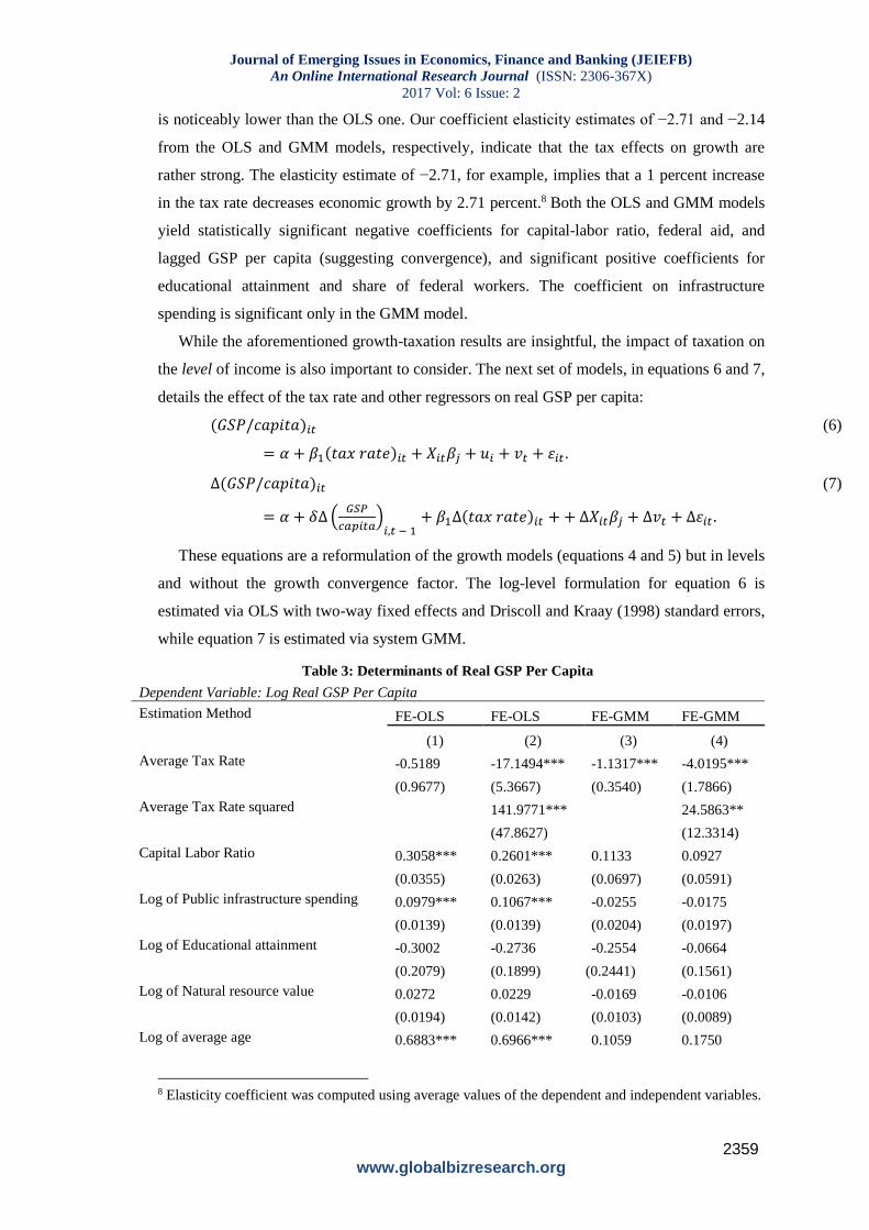
Table 3: Determinants of Real GSP Per Capita

Dependent Variable: Log Real GSP Per Capita

Estimation Method FE-OLS FE-OLS FE-GMM FE-GMM

(1) (2) (3) (4)

Average Tax Rate -0.5189 -17.1494*** -1.1317*** -4.0195***

(0.9677) (5.3667) (0.3540) (1.7866)

Average Tax Rate squared

141.9771***

24.5863**

(47.8627)

(12.3314)

Capital Labor Ratio 0.3058*** 0.2601*** 0.1133 0.0927

(0.0355) (0.0263) (0.0697) (0.0591)

Log of Public infrastructure spending 0.0979*** 0.1067*** -0.0255 -0.0175

(0.0139) (0.0139) (0.0204) (0.0197)

Log of Educational attainment -0.3002 -0.2736 -0.2554 -0.0664

(0.2079) (0.1899) (0.2441) (0.1561)

Log of Natural resource value 0.0272 0.0229 -0.0169 -0.0106

(0.0194) (0.0142) (0.0103) (0.0089)

Log of average age 0.6883*** 0.6966*** 0.1059 0.1750

8 Elasticity coefficient was computed using average values of the dependent and independent variables.





(0.2380) (0.1672) (0.2278) (0.2405)

Federal workers (share of employed) 4.7745 4.0396 4.4516*** 3.4231***

(3.1649) (2.8731) (1.1667) (0.7662)

Federal aid (share of GSP) -0.0001*** -0.0001** -0.0000 -0.0000

(0.0000) (0.0000) (0.0000) (0.0000)

Population density 0.0022*** 0.0023*** 0.0000 0.0001***

(0.0005) (0.0004) (0.0000) (0.0000)

Log Real GSP per capita (t−1)

0.9263*** 0.8982***

(0.0272) (0.0277)

Sargan over-identification test (p-value) 0.62 0.92

Arellano -Bond AR1/AR2 tests (p-

value) 0.96 0.95

Number of Observations 1,568 1,568 1,519 1,519


effects and Driscoll and Kraay (1998) robust standard errors in parentheses, and (2) dynamic system GMM

where endogenous variables are instrumented with own lagged levels and first differences. Constant and

fixed-effects coefficients are not reported. Florida is omitted from the sample due to missing capital and

natural resource data.

The OLS estimate in Column 1, Table 3 reveals that the average tax rate appears to have a

negative but not statistically significant relationship with income levels. However, as

discussed earlier (see Figure 2), there seems to be a “J” shaped relationship between per

capita GSP and average tax rate. When we introduce the square of the average tax rate into

the OLS regression model, the coefficient on the average tax rate turns negative and

significant (see Column 2, Table 3). The coefficient on the squared variable is positive and

significant which is consistent with the relationship depicted in Figure 2. This positive

relationship might be indicative of a possible interdependence (endogeneity) between high

incomes per capita and tax rates.

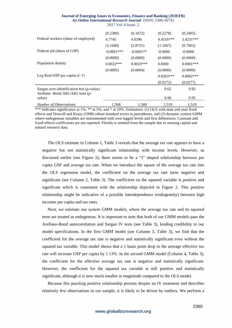
Next, we estimate our system GMM models, where the average tax rate and its squared

term are treated as endogenous. It is important to note that both of our GMM models pass the

Arellano-Bond autocorrelation and Sargan IV tests (see Table 3), lending credibility to our

model specifications. In the first GMM model (see Column 3, Table 3), we find that the

coefficient for the average tax rate is negative and statistically significant even without the

squared tax variable. This model shows that a 1 basis point drop in the average effective tax

rate will increase GSP per capita by 1.13%. In the second GMM model (Column 4, Table 3),

the coefficient for the effective average tax rate is negative and statistically significant.

However, the coefficient for the squared tax variable is still positive and statistically

significant, although it is now much smaller in magnitude compared to the OLS model.

Because this puzzling positive relationship persists despite an IV treatment and describes

relatively few observations in our sample, it is likely to be driven by outliers. We perform a





formal outlier detection test developed by Hadi (1994) and find 11 statistically significant

outliers that belong to the state of Alaska. These observations can be seen as moving away

from the main bulk of the observations and towards the upper right-hand corner in Figure 2.

Due to its heavy reliance on severance taxes, Alaska is often treated as outlier in many fiscal

studies, not surprisingly. When we drop these outlier observations from our sample and re-

estimate the four models in Table 3, we find a negative and statistically significant coefficient

for the effective tax rate across all four models. However, the squared effective tax rate is still

positive and statistically significant in the OLS and GMM models, but with much lower

magnitude than before.

The overall curvature quantified by our estimates means that we are likely measuring all

the effects on the left of the curve where tax rate and per capita GSP are negatively related

given the U.S. conditions. Calculating the inflection points in the OLS and GMM regressions

(see Columns 2&4, Table 3) yields 6% and 8.1% average tax rates, respectively9. Relying on

the GMM model estimates, for example, this implies that the maximum decline in per capita

GSP occurs at the effective average state tax rate of 8.1%. The coefficients on the average tax

rate (in Columns 2&4 in Table 3) show the percentage change in GSP per capita starting from

a point where the average tax variable is equal to zero. As our data does not have any

observations where the average tax rate is equal to zero, we have to exercise caution while

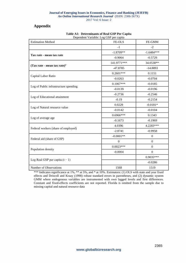
interpreting these coefficients. The econometric solution is to ‘center’ the tax variable and run

a regression with the same set of regressors (including the squared ‘centered’ tax variable).

This also removes any collinearity problems due to using both the average tax rate and its

squared term in the regression10. The coefficients on the centered tax variable now represent

the percentage change in per capita GSP when the average tax rate is at its mean11. Using the

centered coefficients (see Table A1 in the appendix), we calculate that GSP per capita can

change from 1.65% (for GMM) to 1.87% (for OLS) due to 1 basis point change in the average

tax rate of 5.04%. These estimates show that the relationship between GSP per capita and the

average effective tax rate is also economically significant.

While the estimates above suggest that higher effective tax rates reduce state economic

growth and possibly real GSP per capita, they are based on just one metric of economic

activity: state GDP. This metric is not without its flaws and some of the relevant criticisms of

GDP as a measure of economic activity include its failure to account for household

9 Inflection point in the “U” shaped curve is at −

𝛽1

2×𝛽2, where 𝛽1 is the coefficient on the average tax

rate and 𝛽2 is the coefficient on the squared term. 10 Centering the tax variable reduced the correlation with the squared term from 0.985 to 0.19. 11 In our data set the mean average tax rate is approximately 5% (see Table 1 for details). The

regression results with the centered average tax variable is reported in Table A1 in the Appendix.





production, underground markets, environmental quality, and the true value of government

spending (a dollar spent by the government may not generate as much value as a dollar spent

by the private sector, yet both are equally counted in GDP). Overall though, our estimates are

consistent with those of Romer and Romer (2010), who find that an exogenous 1 percent

increase in taxes can decrease real U.S. GDP by 2.5 to 3 percent.

4. Conclusion

This study estimates the impact of the effective average state tax rat on two key measures

of state economic performance: real income per capita and its growth rate in the United

States. Advanced panel data econometric techniques are used to control for endogeneity, non-

linearity, autocorrelation, heteroscedasticity, and contemporaneous correlation. These

attempts improve the odds of capturing a genuine causal relationship between state economic

performance and the effective average tax rate. We find a robust and strong negative

relationship between state economic growth and effective average tax rate. Our estimates are

quantitatively significant and consistent in magnitude with those obtained by Romer and

Romer (2010), who find that an exogenous 1 percent increase in taxes can reduce real GDP

by almost 3 percent. However, the relationship between GSP and the effective average tax

rate appears to be more nuanced. Namely, we find that the effective tax rate may have a non-

linear relationship with GSP per capita. At first, GSP falls as the effective tax rate rises, which

describes most of our observations, but then it begins to rise with the tax rate. This finding

persists even after we instrument for the potentially endogenous tax rate. Our tests suggest

that this positive relationship is mostly due to outliers.

As noted in previous studies, these findings can be sensitive to the choice of time periods,

statistical methods, and regressors. Nonetheless, our findings reveal that a robust and

quantitatively strong negative relationship exists between two different measures of state

economic performance and effective average tax rates during the studied period, even after

controlling for non-linearity and endogeneity. Exploring the nature of taxes at the state level

in the United States is unique as each state has a different set of state taxes that allows us to

make a comparison of the effect of taxes on different states as if they are different countries.

It is important to note that, as emerging economies construct new tax laws to take advantage

of potentially higher tax revenues due to larger incomes, these tax laws are easier to pass than

to repeal. As the volume and complexity of these laws grow each year, they will increasingly

resemble burdensome tax-collecting bureaucracy of the United States. Having a simpler and

lower tax regime can provide creative solutions that may offer opportunities for emerging

countries facing rising income and taxes in the present age of globalization.





References

Alm, J., and Rogers, J. 2011. “Do State Fiscal Policies Affect State Economic Growth?” Public

Finance Review, 39(4): 483–526.

Arellano, M., and Bover, O. 1995. “Another Look at the Instrumental Variable Estimation of Error-

components Models.” Journal of Econometrics, 68: 29–51.

Arin, K. P., Berlemann, M., Koray, F., and Kuhlenkasper, T. 2011. “The Taxation-growth-nexus

Revisited,” HWWI Research Papers 104, Hamburg Institute of International Economics (HWWI).

Bahl, R., and Sjoquist, D. L. 1990. “The State and Local Fiscal Outlook: What Have We Learned and

Where Are We Headed?” National Tax Journal, 43(3): 321–42.

Barro, R. J. 1990. “Government Spending in a Simple Model of Endogenous Growth.” Journal of

Political Economy, 98: S103–S125.

Benson, B. L., and Johnson, R. N. 1986. “The Lagged Impact of State and Local Taxes on Economic

Activity and Political Behavior.” Economic Inquiry, 24(3): 389–401.

Berry, D. M., and Kaserman, D. 1993. “A Diffusion Model of Long-Run State Economic

Development.” Atlantic Economic Journal, 21(4): 39–54.

Besci, Z. 1996. “Do State and Local Taxes Affect Relative State Growth?” Atlanta Federal Reserve

Bank, Economic Review, (March/April): 18–35.

Blundell, R., and Bond, S. 1998. “Initial Conditions and Moment Restrictions in Dynamic Panel-data

Models.” Journal of Econometrics, 87: 115–43.

Canto, V. A., and Webb, R. I. 1987. “The Effect of State Fiscal Policy on State Relative Economic

Performance.” Southern Economic Journal, 54(1): 186–202.

Crain, W. M., and Lee, K. J. 1999. “Economic Growth Regressions for the American States: A

Sensitivity Analysis.” Economic Inquiry, 37(2): 242–57.

Driscoll, J. C., and Kraay, A. C. 1998. “Consistent Covariance Matrix Estimation with Spatially

Dependent Panel Data.” Review of Economics and Statistics, 80: 549–60.

Gale, W.G. and Samwick, A.A., 2016. “Effects of Income Tax Changes on Economic Growth.”

Grossman, P.J., 1988. “Government and economic growth: A non-linear relationship.” Public Choice,

56(2): 193-200.

Hadi, A.S. 1994. “A modification of a method for the detection of outliers in multivariate

samples.” Journal of the Royal Statistical Society. Series B (Methodological): 393-396.

Helms, L. J. 1985. “The Effects of State and Local Taxes on Economic Growth: A Time Series-Cross

Section Approach.” Review of Economics and Statistics, 67(4): 574–82.

Hines, J. 1996. “Altered States: Taxes and the Location of Foreign Direct Investment in America.”

American Economic Review, 86(5): 1076–94.

Jaimovich, N., and Rebelo, S. 2012. “Non-linear Effects of Taxation on Growth.” Working Paper

18473, National Bureau of Economic Research.

Johansson, Å., Heady, C., Arnold, J., Brys, B., & Vartia, L. 2008. “Taxation and economic growth. ”

OECD Economics Department Working Papers, No. 620, OECD Publishing, Paris.

Karagianni, Stella, Maria Pempetzoglou, and Anastasios P. Saraidaris. 2013. “Average Tax Rates and

Economic Growth: A Nonlinear Causality Investigation for the USA.” Frontiers in Finance and

Economics, 12(1): 51-59.

Kocherlakota, N. R., and Yi, K. M. 1997. “Is There Endogenous Long-Run Growth? Evidence from the

United States and the United Kingdom.” Journal of Money, Credit and Banking, 29(2): 235–62.

Koester, R. B., and Kormendi, R. C. 1989. “Taxation, Aggregate Activity and Economic Growth:

Cross-Country Evidence on Some Supply-Side Hypotheses,” Economic Inquiry, 27(3): 367–86.

Laffer, A. B., Moore, S., and Williams, J. 2012. Rich States, Poor States:ALEC-Laffer State Economic

Competitiveness Index, American Legislative Exchange Council, Washington, D.C.





Lee, Y., and Gordon, R. H. 2005. “Tax Structure and Economic Growth.” Journal of Public

Economics, 89: 1027–43.

Lucas, R. 1988. “On the Mechanics of Economic Development.” Journal of Monetary Economics, 22:

3–42.

Mankiw, N. G., Romer, D., and Weil, D. N. 1992. “A Contribution to the Empirics of Economic

Growth.” The Quarterly Journal of Economics, 107(2): 407–37.

Mofidi, A., and Stone, J. A. 1990. “Do State and Local Taxes Affect Economic Growth?” Review of

Economics and Statistics, 72(4): 686–91.

Pjesky, R. 2006. “What Do We Know About Taxes and State Economic Development? A Replication

and Extension of Five Key Studies.” The Journal of Economics, 32(1): 25–40.

Plaut, T. R., and Pluta, J. 1983. “Business Climate, Taxes, and Expenditures, and State Industrial

Growth in the United States.” Southern Economic Journal, 50(1): 99–119.

Poulson, B. W., and Kaplan, J. G. 2008. “State Income Taxes and Economic Growth.” Cato Journal,

28(1): 53–71.

Reed, W. R. 2008. “The Robust Relationship between Taxes and U.S. State Income Growth.” National

Tax Journal, 61(1): 57–80.

Romer, P. 1986. “Increasing Returns and Long-Run Growth.” Journal of Political Economy, 94(2):

1002–37.

Romer, P. 1990. “Endogenous Technological Change.” Journal of Political Economy, 98(5): S71–

S102.

Romer, C. D., and Romer, D.H. 2010. “The Macroeconomic Effects of Tax Changes: Estimates Based

on a New Measure of Fiscal Shocks.” American Economic Review, 100: 763-801.

Smith, A., 1880. An Inquiry Into the Nature & Causes of the Wealth of Nations, Vol 1.

Solow, R. M. 1956. “A Contribution to the Theory of Economic Growth.” The Quarterly Journal of

Economics, 70(1): 65–94.

Tomljanovich, M. 2004. “The Role of State Fiscal Policy in State Economic Growth.” Contemporary

Economic Policy, 22: 318–30.

Turner, C., Tamura, R., Mulholland, S. E., and Baier, S. 2007. “Education and Output of the States of

the United States: 1840–2000.” Journal of Economic Growth, 12: 101–58.

Turner, C., Tamura, R., Schoellman, T., and Mulholland, S. 2011. “Estimating Physical Capital and

Land for States and Sectors of the United States, 1850–2000.” MPRA Paper 32847, University Library

of Munich, Germany.

Vedder, R. K. 2003. Taxation and Migration. Cedarburg, WI: Taxpayers Network, Inc.

Yakovlev, P. 2007. “Arms Trade, Military Spending, and Economic Growth.” Defence and Peace

Economics, 18(4): 317–38.

Yakovlev, P.A., 2014. State Economic Prosperity and Taxation. Working Paper 14-19, Mercatus

Center, George Mason University.

http://ideas.repec.org/s/pra/mprapa.html





Appendix

Table A1: Determinants of Real GSP Per Capita

Dependent Variable: Log GSP per capita

Estimation Method FE-OLS FE-GMM

-1 -2

Tax rate - mean tax rate -1.8709** -1.6484***

-0.9064 -0.5729

(Tax rate - mean tax rate)2 141.9771*** 34.0538**

-47.8785 -14.8893

Capital Labor Ratio 0.2601*** 0.1151

-0.0263 -0.0704

Log of Public infrastructure spending 0.1067*** -0.0185

-0.0139 -0.0196

Log of Educational attainment -0.2736 -0.2546

-0.19 -0.2154

Log of Natural resource value 0.0229 -0.0181*

-0.0142 -0.0104

Log of average age 0.6966*** 0.1343

-0.1673 -0.1969

Federal workers (share of employed) 4.0396 4.2283***

-2.8741 -0.9958

Federal aid (share of GSP) -0.0001** 0

0 0

Population density 0.0023*** 0

-0.0004 0

Log Real GSP per capita (t − 1) 0.9035***

-0.0286

Number of Observations 1568 1519


effects and Driscoll and Kraay (1998) robust standard errors in parentheses, and (2) dynamic system

GMM where endogenous variables are instrumented with own lagged levels and first differences.

Constant and fixed-effects coefficients are not reported. Florida is omitted from the sample due to

missing capital and natural resource data

Documents

State Economic Performance and Effective Tax Ratesglobalbizresearch.org/economics/images/files/44668_ID_1132_JEIEFB... · Journal of Emerging Issues in Economics, Finance and Banking