State-dependent computations: spatiotemporal processing in

All sensory stimuli generate spatiotemporal patterns of action potentials (spikes) that are conveyed to the CNS by sensory afferents. A fundamental goal of neuroscience is to understand how neural networks extract informa-tion from both the spatial and the temporal structure of these complex spike patterns; however, our understand-ing is currently biased towards the processing of spatial information. Indeed, it is not even known whether the spatial and temporal dimensions of stimuli are processed by the same or different networks. Temporal informa-tion is crucial to most forms of sensory processing; for example, in the visual modality, the temporal structure of stimuli is crucial in determining not only the direction and velocity of objects, but also the duration and inter-val between sensory events. In the somatosensory sys-tem, temporal structure contributes not only to motion detection, but also to object and texture discrimina-tion1. However, it is perhaps in the auditory system that temporal processing is most prominent; for example, both the spatial (spectral) and the temporal structure of animal vocalizations — from frog calls to bird song to monkey calls — encode information2. Similarly, speech is rich in spatiotemporal structure, and removing either spatial or temporal information impairs speech recog-nition3,4. The importance of the temporal structure of speech, and the brain’s ability to process complex tem-poral stimuli, is evidenced by the fact that language can essentially be reduced to a single-channel temporal code — as in Morse code. Given the importance of temporal information for the processing of natural stimuli, it is not surprising that neural responses are often strongly dependent on temporal features of stimuli5–7. Indeed,

many neurons respond selectively to specific spatio-temporal stimuli, such as birdsong motifs or patterns of simple stimuli8–12. Together, the universal presence of spatiotemporal patterns in natural stimuli and the sen-sitivity of cortical neurons to spatiotemporal structure argue that any general model of cortical processing must account for the ability of the cortex to process both spatial and temporal information.

How do we discriminate lines of different orienta-tions? Any neuroscience textbook provides an answer to this question by describing the mechanisms that con-tribute to the orientation selectivity of V1 cells to a bar of light. However, the answer to the equally sensible ques-tion ‘How does the brain discriminate between different durations of a bar of light?’ remains largely unanswered. Indeed, relatively few models address this simple ques-tion. Early artificial neural-network models, such as the perceptron13 and later multi-layer perceptron14, proved capable of classifying complex spatial patterns; however, they were ill-suited to performing even a simple interval-discrimination task because there was no representation of time — the patterns being processed were static and not time-varying. Later models processed sequences of spatial patterns by either creating an explicit representa-tion of time by transforming it into an additional spatial dimension (BOX 1), or by taking into account preceding network states through the incorporation of recur-rent connections15–17. It has proved difficult to develop these abstract models into more realistic models that are based on spiking neurons (such as integrate-and-fire neurons) and in which time is continuously represented. In parallel, spiking models of the sensory cortex also

*Departments of Neurobiology and Psychology, and Brain Research Institute, University of California, Los Angeles, California 90095, USA. ‡Institute for Theoretical Computer Science, Graz University of Technology, A‑8010 Graz, Austria.Correspondence to D.V.B.e‑mail: [email protected]:10.1038/nrn2558Published online 15 January 2009

PerceptronA simple linear neuron model that computes a weighted sum of its inputs, and outputs 1 if the weighted sum is larger than some threshold, and 0 otherwise. Weights and thresholds can be learned by the perceptron learning rule.

Multi-layer perceptronA feedforward network of units, the computational function of which is similar to that of a perceptron, except that a smooth function (instead of a threshold) is applied to the weighted sum of inputs at each unit. Weights and thresholds can be learned by the back-propagation learning rule.

State-dependent computations: spatiotemporal processing in cortical networksDean V. Buonomano* and Wolfgang Maass‡

Abstract | A conspicuous ability of the brain is to seamlessly assimilate and process spatial and temporal features of sensory stimuli. This ability is indispensable for the recognition of natural stimuli. Yet, a general computational framework for processing spatiotemporal stimuli remains elusive. Recent theoretical and experimental work suggests that spatiotemporal processing emerges from the interaction between incoming stimuli and the internal dynamic state of neural networks, including not only their ongoing spiking activity but also their ‘hidden’ neuronal states, such as short-term synaptic plasticity.

R E V I E W S

NATurE rEVIEwS | NeuroscieNce VoLuME 10 | fEbruAry 2009 | 113

© 2009 Macmillan Publishers Limited. All rights reserved

mailto:[email protected]

Integrate-and-fire neuronA simple model of a spiking neuron. It integrates synaptic inputs with a passive membrane time constant. Whenever the resulting membrane voltage reaches a firing threshold, it generates an output spike.

RetinotopyA spatial arrangement in which neighbouring visual neurons have receptive fields that cover neighbouring (although partly overlapping) areas of the visual field.

SomatotopyA spatial arrangement in which neighbouring sensory neurons respond to the stimulation of neighbouring receptors in the skin.

focused primarily on spatial processing. These models successfully accounted for the ability of cortical neurons to develop selective responses to the spatial properties of stimuli, such as retinotopy, somatotopy and orienta-tion selectivity18,19. but again, they were not designed to cope with the inherent spatial and temporal structure of natural stimuli.

In this review, we describe a framework in which spatiotemporal computations emerge from the time-dependent properties of neurons and the inherent dynamics in cortical networks20–22. These models posit that spatial and temporal processing are inextricably linked and that information is encoded in evolving neu-ral trajectories (FIG. 1). Thus, in this framework the com-putation is in the voyage through state space as opposed to the destination. Additionally, we examine the predic-tions generated by this framework, including that the state of a network at any point in time encodes not only the present but also the past.

Inputs interact with internal statesThe response of a population of neurons in a network is determined not only by the characteristics of the external stimulus but also by the dynamic changes in the inter-nal state of the network12,21,23–26. In other words, whether a neuron responds to a tone depends not only on the frequency of the tone but also on whether the neuron is receiving additional internally generated excitatory and inhibitory inputs and on the current strength of each

of its synapses (which vary on a rapid timescale). This general point can be intuitively understood by making an analogy between neural networks and a liquid20. A pebble thrown into a pond will create a spatiotemporal pattern of ripples, and the pattern produced by any sub-sequent pebbles will be a complex nonlinear function of the interaction of the stimulus (the pebble) with the internal state of the liquid (the pattern of ripples when the pebble makes contact). ripples thus establish a short-lasting and dynamic memory of the recent stimulus his-tory of the liquid. Similarly, the interaction between incoming stimuli and the internal state of a neural net-work will shape the population response in a complex fashion. However, defining the internal state of a neural network is not straightforward, and it will thus be useful to distinguish between two components, which we will refer to as the active and the hidden states.

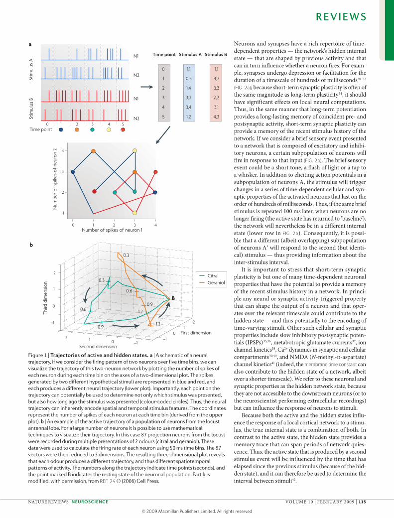
Active and hidden internal states. Traditionally, the internal state of a network is defined as the population of active neurons — we will refer to this as the active state. At any time t we can think of a network of N neurons as an N-dimensional vector that is composed of zeros and ones (depending on the size of the time bin we can also repre-sent each value as a real number representing the firing rate). Such a vector forms a point in N-dimensional space and defines which neurons are active at corresponding time point t. over the course of multiple time bins these points form a path (a neural trajectory) through state space (FIG. 1a). In a network that is driven by an ongoing external stimulus, a complex trajectory will form that represents the temporal evolution of active states. At each point t+1 the response of the neuronal population is dependent not only on the synapses that are directly activated by the input, but also on the ongoing activity in the network: owing to the recurrent nature of cortical circuits, activity in the network provides an additional source of synaptic inputs (the active state from other brain regions can also contribute to the response of a net-work, but from the perspective of any given local network this is equivalent to an additional time-varying input). In vivo recordings demonstrate that different stimuli elicit distinct spatiotemporal patterns of activity24,25,27,28 — that is, different neural trajectories (FIG. 1b, see below). These time-varying changes in the active state can be driven directly by the stimulus structure or by internally gener-ated dynamics produced by the recurrent connectivity. Indeed, in some cases even if the stimulus (for example, a constant odour or steady auditory tone) is not varying in time, the neural trajectories that represent the network’s active state continue to change24,29, which could contrib-ute to computations such as the encoding of intensity or time. for example, because trajectories evolve through time in a reproducible manner for a given stimulus24, any given point has the potential to provide information not only about the stimulus presented but also about time itself — such as how much time has elapsed since the onset of the stimulus (FIG. 1a).

The response of a network is, however, more com-plex than the interaction between the external input and the ongoing pattern of activity in the network.

Box 1 | Spatialization of time

Traditional artificial neural networks, such as the perceptron13 and multi-layer perceptrons14, were designed to process static spatial patterns of inputs — for example, for the discrimination of handwritten characters — and the network structure therefore had no need to implicitly or explicitly incorporate time. When these models began to be used for the discrimination or production of time-varying stimuli, such as speech, the first approach was simply to assume that time was an additional spatial dimension17. For example, in one well-known model that converted written letters into artificial speech105, the input was represented by 26 units (each representing a specific letter of the alphabet) and the temporal context was encoded by dividing time into ‘bins’ and then replicating the input layer of 26 inputs; that is, to encode 7 time bins (t–3, t–2 … t+3) there would be a total of 182 (26×7) inputs to the network. As the simulation progressed this 7-bin time window would slide forward bin by bin. In essence, time was ‘spatialized’ by transforming it into an additional spatial dimension. A spatial representation of time was also used in more biology-based models, such as those that simulated the fact that many forms of classical conditioning generated motor responses at the appropriate point in time; such ‘delay-line’ or ‘labelled-line’ models assume that in response to a stimulus specific neurons will respond with specific hardwired delays106–108. Biologically speaking it is clear that time is not treated as an additional spatial dimension at the level of the inputs — that is, the sensory organs. However, in the CNS there is likely to be a spatial representation of some temporal features, particularly simple features such as the interval between two events. Thus, the question is not whether time can be centrally represented in a spatial code, but how this is achieved.

A second approach in artificial neural-network models was to implicitly represent time using recurrent connections, which allowed the state of the previous time step to interact with the input from the current time step, thus providing temporal context15,17. These networks still treated time as a discrete dimension composed of time bins that were updated according to a centralized clock; the units themselves were devoid of any temporal properties. Together, these features have made these models difficult to generalize to biologically realistic continuous time models composed of asynchronous spiking neurons.

R E V I E W S

114 | fEbruAry 2009 | VoLuME 10 www.nature.com/reviews/neuro


Nature Reviews | Neuroscience

10 2 3 4

1

2

3

4

Number of spikes of neuron 1

Num

ber o

f sp

ikes

of n

euro

n 2

a

Stim

ulus

B

N1

N2

N1

N2

Time point0 1 2 3 4 5

Stim

ulus

A

1,1

4,2

3,3

2,2

3,1

4,3

1,1

0,3

1,4

3,2

3,4

1,2

Time point

0

1

2

3

4

5

Stimulus A Stimulus B

b

Third

dim

ensi

on

Second dimension

First dimension

–1

–1–1

0

2

1

2

2

1

1

0

00.9

0.6

0.6

0.3

0.9

0.3

B

1.2

1.2

CitralGeraniol

Neurons and synapses have a rich repertoire of time-dependent properties — the network’s hidden internal state — that are shaped by previous activity and that can in turn influence whether a neuron fires. for exam-ple, synapses undergo depression or facilitation for the duration of a timescale of hundreds of milliseconds30–33 (FIG. 2a); because short-term synaptic plasticity is often of the same magnitude as long-term plasticity34, it should have significant effects on local neural computations. Thus, in the same manner that long-term potentiation provides a long-lasting memory of coincident pre- and postsynaptic activity, short-term synaptic plasticity can provide a memory of the recent stimulus history of the network. If we consider a brief sensory event presented to a network that is composed of excitatory and inhibi-tory neurons, a certain subpopulation of neurons will fire in response to that input (FIG. 2b). The brief sensory event could be a short tone, a flash of light or a tap to a whisker. In addition to eliciting action potentials in a subpopulation of neurons A, the stimulus will trigger changes in a series of time-dependent cellular and syn-aptic properties of the activated neurons that last on the order of hundreds of milliseconds. Thus, if the same brief stimulus is repeated 100 ms later, when neurons are no longer firing (the active state has returned to ‘baseline’), the network will nevertheless be in a different internal state (lower row in FIG. 2b). Consequently, it is possi-ble that a different (albeit overlapping) subpopulation of neurons A′ will respond to the second (but identi-cal) stimulus — thus providing information about the inter-stimulus interval.

It is important to stress that short-term synaptic plasticity is but one of many time-dependent neuronal properties that have the potential to provide a memory of the recent stimulus history in a network. In princi-ple any neural or synaptic activity-triggered property that can shape the output of a neuron and that oper-ates over the relevant timescale could contribute to the hidden state — and thus potentially to the encoding of time-varying stimuli. other such cellular and synaptic properties include slow inhibitory postsynaptic poten-tials (IPSPs)35,36, metabotropic glutamate currents37, ion channel kinetics38, Ca2+ dynamics in synaptic and cellular compartments39,40, and NMDA (N-methyl-d-aspartate) channel kinetics41 (indeed, the membrane time constant can also contribute to the hidden state of a network, albeit over a shorter timescale). we refer to these neuronal and synaptic properties as the hidden network state, because they are not accessible to the downstream neurons (or to the neuroscientist performing extracellular recordings) but can influence the response of neurons to stimuli.

because both the active and the hidden states influ-ence the response of a local cortical network to a stimu-lus, the true internal state is a combination of both. In contrast to the active state, the hidden state provides a memory trace that can span periods of network quies-cence. Thus, the active state that is produced by a second stimulus event will be influenced by the time that has elapsed since the previous stimulus (because of the hid-den state), and it can therefore be used to determine the interval between stimuli42.

Figure 1 | Trajectories of active and hidden states. a | A schematic of a neural trajectory. If we consider the firing pattern of two neurons over five time bins, we can visualize the trajectory of this two-neuron network by plotting the number of spikes of each neuron during each time bin on the axes of a two-dimensional plot. The spikes generated by two different hypothetical stimuli are represented in blue and red, and each produces a different neural trajectory (lower plot). Importantly, each point on the trajectory can potentially be used to determine not only which stimulus was presented, but also how long ago the stimulus was presented (colour-coded circles). Thus, the neural trajectory can inherently encode spatial and temporal stimulus features. The coordinates represent the number of spikes of each neuron at each time bin (derived from the upper plot). b | An example of the active trajectory of a population of neurons from the locust antennal lobe. For a large number of neurons it is possible to use mathematical techniques to visualize their trajectory. In this case 87 projection neurons from the locust were recorded during multiple presentations of 2 odours (citral and geraniol). These data were used to calculate the firing rate of each neuron using 50 ms time bins. The 87 vectors were then reduced to 3 dimensions. The resulting three-dimensional plot reveals that each odour produces a different trajectory, and thus different spatiotemporal patterns of activity. The numbers along the trajectory indicate time points (seconds), and the point marked B indicates the resting state of the neuronal population. Part b is modified, with permission, from REF. 24 (2006) Cell Press.

R E V I E W S




‘Rest’ state Active state (t = 1 ms)

a

b

0 ms 20 ms 40 ms 60 ms 80 ms 100 ms

Active state (t = 101 ms)‘Hidden’ state (t = 99 ms)

10 Hz

20 Hz

40 Hz

1 mV

50 ms

10 Hz

20 Hz

40 Hz

1 mV

50 ms

Inputs

Inhibitory neurons

Excitatoryneurons

Membrane time constantA physical measure that reflects the time it takes the voltage of a neuron to achieve 63% of its final value for a steady-state current pulse.

Figure 2 | Active and hidden network states. a | An example of short-term plasticity of excitatory postsynaptic potentials (EPSPs) in excitatory synapses between layer 5 pyramidal neurons. Short-term plasticity can take the form of either short-term depression (left) or short-term facilitation (right). The plots show that the strength of synapses can vary dramatically as a function of previous activity, and thus function as a short-lasting memory trace of the recent stimulus history. The traces represent the EPSPs from paired recordings; each presynaptic action potential is marked by a dot. b | Hidden and active states in a network. The spheres represent excitatory (blue) and inhibitory (red) neurons, and the arrows represent a small sample of the potential connections. The baseline state (‘rest’ state, top left panel) is represented as a quiescent state (although in reality background and spontaneous activity must be taken into account). In the presence of a brief stimulus the network response will generate action potentials in a subpopulation of the excitatory and inhibitory neurons (light shades), which defines the active state of the network (top right panel). After the stimulus, the neurons in early cortical areas stop firing. However, as a result of short-term synaptic plasticity (represented by dashed lines) and changes in intrinsic and synaptic currents (represented by different colour shades), the internal state may continue to change for hundreds of milliseconds. Thus, although it is quiescent, the network should be in a different functional state at the time of the next stimulus (at t = 100 ms) — this is referred to as the ‘hidden’ state (bottom left panel). The fact that the network is in a different state implies that it should generate a different response pattern to the next stimulus (bottom right panel), even if the stimulus is identical to the first one (represented as a different pattern of blue spheres). Part a is reproduced, with permission, from REF. 31 (1999) Society for Neuroscience.

R E V I E W S



Liquid-state machineA class of computational model that is characterized by one or several read-outs applied to some generic dynamical system, such as a recurrent network of spiking neurons. Whereas the dynamical system contributes generic computational operations, such as fading memory and nonlinear combinations of features that are independent of concrete computational tasks, each read-out can be trained to extract different pieces of the information that is accumulated in the dynamical system.

Echo-state networkA class of artificial neural network model that is based on recurrent connections between analogue units, in which the connection weights are random but appropriately scaled to generate stable internal dynamics. These models can encode temporal information as a result of the active state but do not have hidden states.

State-dependent networkA class of model that is based on the characteristics described in this Review. The state-dependent network model proposes that cortical networks are inherently capable of encoding time and processing spatiotemporal stimuli as a result of the state-dependent properties imposed by ongoing activity (the active state) and as a result of time-dependent neural properties (the hidden states).

Reservoir computingA general term used primarily in machine learning to refer to models that rely on mapping stimuli onto a high-dimensional space in a nonlinear fashion. Such models include echo-state machines, liquid-state machines and state-dependent networks.

Linear discriminatorA type of classifier that can be computed by a perceptron.

Synaptic weightsThe strength of synaptic connections between neurons.

The interaction between internal states and time- varying external inputs has been proposed to be a key step in cortical function20–22,29,43. Some theoretical mod-els, with varying degrees of biological plausibility, have relied on this principle for the processing of spatio-temporal stimuli. In some of the models, the encoding of past stimuli was based solely on ongoing changes in the active state produced by the recurrent architecture17,44–47. In other models, the memory of previous events was con-tained in the active and/or hidden states20,22,42,48,49. In the context of neuroscience and machine learning, several instantiations of the general framework discussed in this review have emerged, including liquid-state machines20,50, echo-state networks45, state-dependent networks2,22 and reservoir computing51. As is explained in the next sec-tion, a key result that arises from these models is that trajectories of active network states can, in spite of their complexity, be used for noise-robust computations on time-varying external inputs.

Decoding neural trajectoriesIn response to a stimulus, the active state of a network of neurons typically changes on a fast timescale of tens of milliseconds. How can downstream systems extract use-ful information about the external stimulus, such as the identity of an odour or of a spoken word, from these trajectories of transient states?

This decoding problem becomes less formidable if one considers it from the perspective of a down-stream or ‘read-out’ neuron. read-out neurons, which extract information from upstream areas and project it to downstream systems, are typically contacted by a large set of input neurons — thus each read-out neuron receives a high-dimensional sample of the active state of the upstream network. from a theoretical perspective, the high-dimensionality of the sample space facilitates the extraction of information by read-out neurons (see below). Let us assume for simplicity that read-out neu-rons are modelled by perceptrons — that is, that they have the discrimination capability of a linear discriminator. Such a linear discriminator, when applied to a point x1, x2 … xd from a d-dimensional state space (which corre-sponds to the active state of a population of d presynaptic neurons), computes a weighted sum w1x1 + w2x2 + … wdxd at each time point, where w1, w2 … wd are the weights of the discriminator (corresponding to the synaptic weights of each presynaptic input); it outputs 1 whenever the weighted sum is above the threshold, and 0 otherwise. In this fashion, linear read-out neurons can classify the time-varying active states of presynaptic neurons accord-ing to the external stimuli that caused these active states — in other words, the read-out neurons become a detec-tor, in that their activity reflects the presence of a specific stimulus. An example of such a separation of trajectories of active states is shown in FIG. 3.

robust separation of the trajectories is difficult in few dimensions (that is, few presynaptic inputs) (see BOX 2 figure, part a), but mathematical results demonstrate that a linear separation of trajectories becomes much easier when the state space has many dimensions (see BOX 2 figure, part b). In particular, linearly inseparable

classes of external stimuli tend to become linearly sepa-rable once they are projected nonlinearly into a higher-dimensional state space52 (BOX 2). The nonlinearity of the projection of stimuli into high-dimensional space is a product of the inherent complexity and nonlinear nature of the interaction between the internal state and external stimuli. Indeed, from a theoretical perspective64 it is not the precise nature of the transformation itself, but rather the increase in the dimensionality of the represen-tation that is crucial to the computation. As mentioned above, because a typical read-out neuron in a cortical area receives synaptic input from thousands of neurons, it has a high likelihood of being able to separate the trajectories of active states of its presynaptic neurons according to the external stimuli that caused these trajectories.

Can read-out neurons learn to decode time-varying active states? Experimental and theoretical results to date indicate that read-out neurons are in principle able to separate complex trajectories of active states of pre synaptic neurons if their synaptic weights are deter-mined by a suitable learning rule (see below)44,53–55. It remains unknown, however, whether the appropriate set of synaptic weights can be learned in vivo.

In the case in which a read-out neuron is modelled by a linear discriminator, if one assumes that the read-out neuron is informed during learning which trajectory resulted from stimulus class A and which from class b (a process known as supervised learning), then traditional learning rules (such as the perceptron learning rule or backpropagation)13,56 converge to a weight vector that achieves the desired separation — provided that such a set of weights exists. Traditional artificial neural net-work learning rules do not capture information that is contained in previous time steps — that is, information encoded in the temporal pattern of active states; how-ever, some supervised-learning rules have also proved effective in allowing spiking read-out neurons to extract information from the spatiotemporal pattern of inputs generated by different stimuli57.

Additionally, it is plausible that a biological read-out neuron can learn to decode the active states of a recurrent network through trial and error in a reward-based setting. for example, it has been shown that reward-modulated spike timing-dependent plasticity (STDP) allows spiking neurons to learn to discriminate different trajectories using reinforcement learning58,59 — a form of learning in which the animal or network receives a global positive or negative feedback signal based on its performance.

In a third model for decoding spatial or spatio-temporal patterns of activity, read-out neurons learn to separate trajectories in the absence of a ‘teacher’ and of rewards — that is, in an unsupervised fashion. one such model, termed slow-feature analysis, takes advantage of the observation that stimuli remain present on time-scales that generally exceed those over which the neural trajectories are changing. It has been shown that a spik-ing read-out neuron can learn through STDP to extract the slow features from the trajectory of active states of presynaptic neurons under certain conditions60. This approach has been applied to unsupervised learning of

R E V I E W S




kHz

a

b

c

e

d

Inpu

t

Inpu

t

Recu

rren

t ne

twor

k

Recu

rren

t ne

twor

k

0

20

30

40

10

0

40

60

80

20

0 100 200 300 0 100 200 300

Time (ms) Time (ms)

0 100 200 300 0 100 200 300Time (ms) Time (ms)

Forward Reverse

100 200 300

2

0

–2

Time (ms)

8642

5

5

0–2–4

–5 –10–15 15 10

–6–8

00

8642

5

5

0–2–4

–5 –10–15 15 10

–6

–80

0

10

10

–10–10–15

5

5

5

–5

–5

–5

0

0

0

10

10

–10–10–15

5

–55

5

–5

–5

0

0

0

Read

-out

Read-out neuron

Excitatory neuron

Inhibitory neuron

Input neuron

0

40

60

80

20

0

20

30

40

10

0 ms

350 ms

4

3

2

1

R E V I E W S



Learning ruleA rule that governs the relationship between patterns of pre- and postsynaptic activity and long-term changes in synaptic strength. For example, spike timing-dependent plasticity.

Recurrent networkA network in which any neuron can be directly or indirectly connected to any other — the flow of activity from any one initial neuron can propagate through the network and return to its starting point. By contrast, in a feedforward network information cannot return to the point of origin.

Spike timing-dependent plasticity(STDP). Traditionally, a form of synaptic plasticity in which the order of the pre- and postsynaptic spikes determines whether synaptic potentiation (pre- and then postsynaptic spikes) or depression (post- and then presynaptic spikes) ensues.

invariant pattern classification of moving visual inputs by linear discriminators61.

A question related to how read-out neurons learn to respond in a stimulus-specific manner is whether the read-out neurons exhibit robust generalization — indeed, the ability to properly respond to a novel stimulus and to similar instances of the same stimulus is fundamental for effective sensory processing. Theoretical results from statistical learning theory62 imply that linear read-outs exhibit better generalization than highly nonlinear neu-rons, because they have fewer degrees of freedom during learning63. Analysis of network properties that favour robust generalization of trained read-outs to new net-work inputs shows that a necessary and sufficient condi-tion for generalization is that the inputs that need to be classified differently by a read-out neuron result in tra-jectories that stay farther apart than two trajectories that are caused by two trials with the same external input64.

It should be noted that to date there is little direct experimental evidence regarding how neurons in vivo learn to extract information from upstream areas. However, the theoretical work reviewed above suggests that variations on experimentally described forms of synaptic plasticity could in principle suffice. finally, it should be pointed out that models related to the frame-work described here — in which linear discriminators are used to read out information from complex recurrent artificial neural networks — have proved to be a power-ful tool in engineering and machine-learning applica-tions, such as time series prediction, speech classification and handwriting recognition45,51.

Noise, chaos and network dynamics. In vivo recordings demonstrate that there is significant variability in net-work activity in response to nominally identical experi-mental trials25. for example, FIG. 4b shows the variability of spike trains from a neuron in the primary visual cor-tex for 50 trials in which exactly the same visual stimu-lus was shown to an anaesthetized cat. This variability is generally attributed to internal noise and different ini-tial internal states. In the context of recurrent networks, noise can reduce the ability to encode information about past stimuli (the memory span). furthermore, theoreti-cal and modelling studies have shown that recurrent net-works can exhibit chaotic behaviour64–69 — specifically, in simulations the removal of a single spike can cause large changes in the subsequent spiking activity67.

Computational models of recurrent networks establish that certain regimes — particularly when the strength of recurrent connections dominates network dynamics — can be highly sensitive to noise and exhibit chaotic behaviour66,67. However, it is clear that cortical neural networks, although they are recurrent, are not chaotic in the sense that trajectories of neural states are not dominated by noise24,25,53,70. for example, in the experiment described in FIG. 4, a read-out unit (FIG. 4c) could determine from a single trial not only the identity of the current stimulus but also that of a past stimulus that is no longer present, despite the noise in the system. How the brain creates these non-chaotic states in recur-rent networks is a fundamental issue that remains to be fully addressed.

However, it is known that the complex dynamics that are associated with chaotic regimes can be avoided by appropriately scaling the synaptic weights45,47,64. furthermore, numerous computational models have shown robust pattern recognition in the presence of noise using recurrent networks and linear read-outs20,22,48,71–73. Additional theoretical work shows that under certain conditions randomly connected networks can encode past information in the ongoing dynamics of the active states, and the duration of this fading memory increases with network size74,75. In addressing the influence of noise on the framework described here, it is important to con-sider a number of other factors. first, the external stimu-lus can limit the sensitivity of the neural network to noise because it also actively shapes the neural trajectory, and can in effect entrain the dynamics. Indeed, the relative strength of the recurrent connections in relation to the input connections is crucial to determining the behaviour of the network. Notably, the recurrent connections do not need to be strong enough to generate self-maintaining activity in order to contribute to spatiotemporal compu-tations: during the presentation of time-varying stimuli even weak recurrent connections provide an interaction between the current and immediately preceding sensory events. Second, for time spans over which sensory infor-mation is often integrated (hundreds of milliseconds), generic models of recurrent cortical microcircuits can store information about past stimuli50,75. Third, theoreti-cal analyses generally do not take into account the contri-bution of the hidden states. Specifically, time-dependent properties, such as short-term synaptic plasticity and

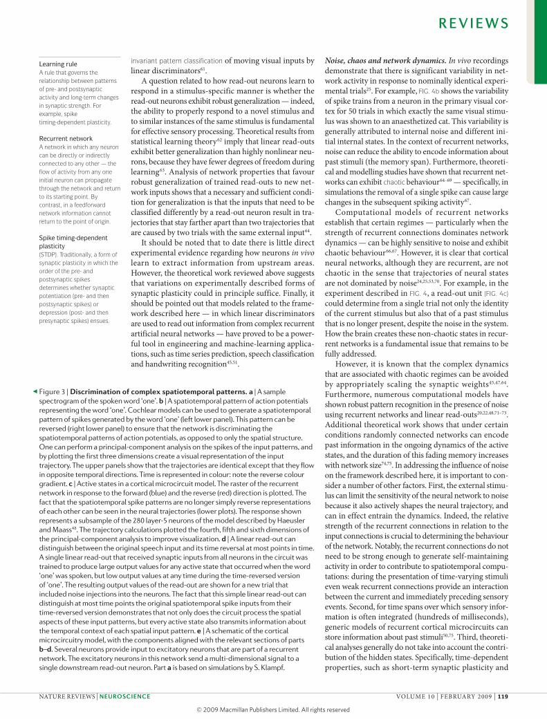
Figure 3 | Discrimination of complex spatiotemporal patterns. a | A sample spectrogram of the spoken word ‘one’. b | A spatiotemporal pattern of action potentials representing the word ‘one’. Cochlear models can be used to generate a spatiotemporal pattern of spikes generated by the word ‘one’ (left lower panel). This pattern can be reversed (right lower panel) to ensure that the network is discriminating the spatiotemporal patterns of action potentials, as opposed to only the spatial structure. One can perform a principal-component analysis on the spikes of the input patterns, and by plotting the first three dimensions create a visual representation of the input trajectory. The upper panels show that the trajectories are identical except that they flow in opposite temporal directions. Time is represented in colour: note the reverse colour gradient. c | Active states in a cortical microcircuit model. The raster of the recurrent network in response to the forward (blue) and the reverse (red) direction is plotted. The fact that the spatiotemporal spike patterns are no longer simply reverse representations of each other can be seen in the neural trajectories (lower plots). The response shown represents a subsample of the 280 layer-5 neurons of the model described by Haeusler and Maass48. The trajectory calculations plotted the fourth, fifth and sixth dimensions of the principal-component analysis to improve visualization. d | A linear read-out can distinguish between the original speech input and its time reversal at most points in time. A single linear read-out that received synaptic inputs from all neurons in the circuit was trained to produce large output values for any active state that occurred when the word ‘one’ was spoken, but low output values at any time during the time-reversed version of ‘one’. The resulting output values of the read-out are shown for a new trial that included noise injections into the neurons. The fact that this simple linear read-out can distinguish at most time points the original spatiotemporal spike inputs from their time-reversed version demonstrates that not only does the circuit process the spatial aspects of these input patterns, but every active state also transmits information about the temporal context of each spatial input pattern. e | A schematic of the cortical microcircuitry model, with the components aligned with the relevant sections of parts b–d. Several neurons provide input to excitatory neurons that are part of a recurrent network. The excitatory neurons in this network send a multi-dimensional signal to a single downstream read-out neuron. Part a is based on simulations by S. Klampf.

◀

R E V I E W S




a

b 1.0

0.5

0.0

20

10

Prob

abili

ty

Ave

rage

min

imum

dist

ance

0 200 400 600 800 1,000

Dimension (d)Invariant pattern classificationThe discrimination of patterns in a manner that is invariant across some transformation. For example, recognition of the same word spoken at different speeds or by different speakers.

ChaosIn theoretical work this term is applied only to deterministic dynamical systems without external inputs, and characterizes extreme sensitivity to initial conditions. In neuroscience it is also applied more informally to systems that receive ongoing external inputs (and that are subject to noise and hence are not deterministic), and characterizes neuronal systems with a trajectory of neural states that is strongly dependent on noise and less dependent on external stimuli.

HyperplaneA hyperplane is a generalization of the concept of a plane in a three-dimensional space to d-dimensional spaces for arbitrary values of the dimension d. A hyperplane in d dimensions splits the d-dimensional space into two half spaces.

slow IPSPs, also provide a memory on the timescale of hundreds of milliseconds. This memory is likely to contribute to the representation of past information in a fashion that is less susceptible to noise because it is not necessarily amplified as a result of the positive feedback that is inherent to recurrent connectivity. for example, as mentioned above, sensory cortical areas do not generally exhibit self-maintaining activity, and after a brief stimulus they return to low-level firing rates; in these cases the hidden state can provide a memory that bridges the gap between stimuli42,76, and this memory should be relatively insensitive to noise as the network is silent.

Most theoretical analyses of dynamics have considered recurrent networks in which both the connectivity and the weights are randomly assigned. However, given the universal presence of synaptic plasticity77,78 and known connectivity data79,80, it is clear that synaptic connectivity and strengths are not random in cortical circuits. Indeed, one of the fundamental features of the cortex is the fact that synaptic strength and neural circuit structure are modified as a function of sensory experience81–84. These forms of long-term and experience-dependent plas-ticity probably play a crucial part in shaping network dynamics and producing stable and reproducible neural

Box 2 | Encoding in high dimensions

Consider two neural trajectories, TA and T

B, in d dimensions

(see the figure, part a), both of which are defined as paths that linearly connect sets of N randomly drawn points in the d-dimensional hypercube [0,1]d. A point x in this space represents the active state of presynaptic neurons at a specific time point t. Its ith coordinate could represent, for example, the firing rate of the ith presynaptic neuron in a time bin centred at t. An alternative method for representing the contribution of presynaptic neuron i is to convolve the spike train of neuron i with an exponential function (for example, an exponentially decaying kernel with a time constant of 20 ms) and take the output value of the resulting linear filter at time t (scaled into [0,1]) as the ith component of the active state55.

The read-out of the active states can be modelled by a perceptron15,109, which computes a weighted sum w

1x

1 + w

2x

2 + … w

dx

d of the inputs x. Geometrically, those

points (x1, x

2 … x

d) at which the weighted sum is exactly

equal to the threshold form a hyperplane in the d-dimensional input space. Such a hyperplane is shown as a grey surface in part a of the figure for the case d = 3, together with a trajectory T

A (the green curve) and a

trajectory TB (the blue curve). The linear discriminator

assigns the output value 1 to the points on one side of the hyperplane, where the weighted sum is larger than the threshold, and 0 to the points on the other side. The values of the weights and the threshold of the linear discriminator define the position of this hyperplane. Complete separation of T

A and T

B would imply that there is a linear

read-out that could output the value 1 for all points in TA,

and the value 0 for all points in TB. This extreme case is

illustrated for d = 3 in part a of the figure. However, such perfect separation can in general not be expected (for example, a read-out neuron might not be able to separate presynaptic active states in a reliable manner immediately after stimulus onset), and it suffices if the hyperplane separates the trajectories during some given time window.

Although robust separation of complex trajectories is difficult in low dimensions, results from mathematical theory imply that a linear separation of trajectories becomes much easier when the dimension of the state space exceeds the ‘complexity’ of the trajectories52. Part b of the figure shows that most pairs of trajectories defined by paths through any 2 sequences of 100 points can be separated by a linear discriminator as the dimension d becomes larger than 100. The probability that 2 trajectories that each linearly connect 100 randomly chosen points can be separated by a hyperplane is plotted in black. The green curve gives the average of the minimal Euclidean distance between pairs of trajectories. It shows that the distance between any two such trajectories tends to increase as d grows. Thus, at higher dimensions not only is it more likely that any two such trajectories can be separated, but also they can be separated by a hyperplane with a larger ‘safety margin’. A larger margin implies that noisy perturbations of these two trajectories can be classified by the linear discriminator in the same way as the original trajectories. One should note that projections of external inputs into higher-dimensional networks are quite common in the brain. For example, ~1 million axons from the optic nerve inject visual information from the lateral geniculate nucleus into the primary visual cortex, in which there are ~500 million neurons. Thus, the primary visual cortex gives rise to trajectories in a much higher dimensional space than those generated by the retinal ganglion cells. Theoretical results64 suggest that the way these trajectories are generated is not all that important for the resultant computational capability of the network: it is primarily the linear dimension of the space that is spanned by the resulting trajectories that is crucial.

R E V I E W S




10

0 0

20

30

40

50

Tria

l ind

ex

Tria

l ind

exb

10

20

30

40

50

a

0

400PSTH PSTH

400

0 200 400 600

10

20

30

40

50

60

c

Time (ms)

Uni

t in

dex

10

20

30

40

50

60

Σ

0

20

40

60

80

100

0 100–100 200 300 400 500 600 7000

80

Mea

n fir

ing

rate

(Hz)

Time (ms)

d

0 200 400 600

S

D

A B C BB C

Time (ms)

0

A D

Perf

orm

ance

(% c

orre

ct)

B

BB CA D B

A B C BB CB

Figure 4 | Population activity from the cat visual cortex encodes both the current and previous stimuli. a | A sample stimulus, with the receptive fields (squares) of the recorded neurons superimposed. b | The spike output of neuron number 10 for 50 trials with the letter sequence A, B, C as the stimulus and 50 trials with the letter sequence D, B, C as the stimulus. The temporal spacing and duration of each letter is indicated through green shading. The lower plot is a post-stimulus time histogram (PSTH) showing the response of neuron 10 (shown in blue in part c) over the 50 trials shown. c | The spike response of 64 neurons during trial number 38 (indicated in blue in part b) for the letter sequence A, B, C (left-hand plot), and the read-out mechanism that was used to decode information from these 64 spike trains (upper right-hand plot). Each spike train was low-pass filtered with an exponential and sent to a linear discriminator. Traces of the resulting weighted sum are shown in the lower right-hand plot both for the trajectory of active states resulting from stimulus sequence A, B, C (black trace) and for stimulus sequence D, B, C (orange trace). For the purpose of classifying these active states, a subsequent threshold was applied. The weights and threshold of the linear discriminator were chosen to discriminate active states resulting from letter sequence A, B, C and those resulting from the letter sequence D, B, C. The blue traces in parts b and c show the behaviour of neuron 10. d | The performance of a linear discriminator at various points in time. The red line shows the percentage of the cross-validated trials that the read-out correctly classified as to whether the first stimulus was A or D. The read-out neuron contained information about the first letter of the stimulus sequence even several hundred milliseconds after the first letter had been shown (and even after a second letter had been shown in the meantime). Note that discrimination is actually poor during the A and D presentation because of the low average firing rate (blue dashed lines). Part a is reproduced, with permission, from REF. 55 (2007) MIT Press. Parts b–d are partly based on data from REF. 55.

R E V I E W S



AttractorThe state of a dynamical system to which the system converges over time, or the state that ‘attracts’ neighbouring states.

Sparse codeA neural code in which only a small percentage of neurons is active at any given point in time.

trajectories that improve the encoding and read-out of behaviourally relevant stimuli. Effectively incorporating plasticity into recurrent networks that are composed of spiking neurons has proved to be a challenge, but recent studies have shown that certain learning rules can help to embed neural trajectories in recurrent networks85, and work on reward-modulated STDP58,59,86 has also begun to address this issue. Additionally, it has been shown that the time span over which networks can encode previous events can be increased in models with spiking neurons through long-term synaptic plasticity71.

Computing with trajectoriesThe framework reviewed above proposes that cortical networks are inherently capable of processing complex spatiotemporal stimuli as a result of the interaction between external stimuli and the state of the internal network. Additionally, it suggests that sets of read-out neurons can extract information from the time-varying neural trajectories represented in high-dimensional space. As was recently stressed by a number of groups21,29,87, this notion marks a significant departure from the traditional hypothesis that cortical computa-tions rely on neural networks that converge to steady-state attractors88,89 — that is, states in which neural firing rates remain constant for a minimal period of time. Although there is evidence that in higher-order cortical areas these fixed-point attractors play a part in working memory90–92, few data suggest that they contribute to the pattern recognition of complex time-varying stimuli. Thus, earlier cortical areas, the computational task of which is to decide what stimulus is present, could extract information from neural trajectories. This framework is well suited to the fact that most complex forms of sen-sory processing take place in real-time in the presence of ever-changing sensory stimuli.

we next review experimental data from different neural systems that support the notion that neural com-putations arise from state-dependent computations and are represented in the trajectory of the active states in high-dimensional space.

Olfactory system. The mechanism that underlies the discrimination and coding of olfactory information has proved to be a valuable system for the study of neural dynamics in recurrent circuits93. Studies in the locust sug-gest that even when it is presented for a prolonged period, a given odour is encoded in a characteristic trajectory of active states (FIG. 1b). Specifically, the projection neurons (PNs) in the antennal lobe exhibit complex time-varying changes in firing rate in response to a tonic stimulus. for each odour, a complex spatiotemporal pattern is formed across the approximately 800 recurrently connected projection neurons that represents a trajectory in a high-dimensional space53. The trajectory is reproducible for a given odour at a given concentration. This trajectory can evolve for a few seconds and then converge to a fixed point. The cells that are located in the next processing stage — the Kenyon cells in the mushroom bodies — create a sparse code of olfactory stimuli that also changes with time. furthermore, the Kenyon cells, which can be

thought of as read-outs of the PNs, decrease their fir-ing when the active state of the PNs has converged to an attractor. That is, the Kenyon cells, which transmit the ‘output’ of the computation of the PNs, respond preferentially while the PN trajectory is in motion but respond less when it is in the steady state. Additionally, as it can take up to a few seconds for the fixed point to be achieved, the fixed point is unlikely to contribute to behavioural decisions in vivo. Consistent with the predic-tions of the framework discussed above, the response of the network to an odour b was distinct from the response to the same odour when it was preceded by odour A24, reflecting the state dependency of the trajectory of the active states of PNs and suggesting that the network has the potential to encode not only the current stimulus but also past stimuli. The fact that the neural trajectories are dynamic even when the stimulus is not suggests that the internal dynamics have a critical role in the ongoing com-putations29. Together, these results provide experimental evidence that the critical computation in olfactory dis-crimination resides in the voyage of the network through high-dimensional state space, as opposed to it residing in the arrival at a specific location in state space.

Timing in the cerebellum. Experimental evidence suggests that the cerebellum regulates some types of motor timing94,95. Although the mechanisms that under-lie timing are not fully understood, it has been shown that small lesions in the cerebellar cortex can alter the timing of a motor response96. Consistent with these findings, it has been proposed that timing relies on the spatio-temporal dynamics of the granule cell population and that these dynamics arise from the interaction between cerebellar input and the internal state of the cerebellar network44,97. In the cerebellum, granule and Golgi cells are part of a negative-feedback loop in which granule cells excite Golgi cells, which in turn inhibit granule cells. In response to a constant stimulus, conveyed by the mossy fibres, the granule cell population response is not only a function of the current stimulus, but also depends on the current state of the granule cell–Golgi cell net-work. Simulations reveal that, as a result of the feed-back loop, a dynamically changing trajectory of active granule cells is created in response to a stimulus44,46,98. This pattern will trace a complex trajectory in neuron space, and as each point of the trajectory corresponds to a specific population vector of active granule cells, the network inherently encodes time. Time can then be read out by the Purkinje cells (the ‘read-out’ neurons), which sample the activity from a large population of granule cells. Importantly, the Purkinje cells can learn to gener-ate timed motor responses through conventional asso-ciative synaptic plasticity coupled to the reinforcement signal from the inferior olive99. In this framework, the pattern of granule cell activity would be expected not only to encode all potentially relevant stimuli, but also to be capable of generating a specific time stamp of the time that has elapsed since the onset of each potential stimu-lus. This scheme clearly requires a very high number of distinct granule cell patterns. Indeed, the fact that there are over 5×1010 granule cells in the human cerebellum100

R E V I E W S



PsychophysicsStudies based on perceptual decisions regarding the physical characteristics of stimuli, such as the intensity or duration of sensory stimuli.

TonotopyA spatial arrangement in which tones that are close to each other in terms of frequency are represented in neighbouring auditory neurons.

suggests that they are uniquely well suited and indeed designed to encode the large number of representations that would arise from having to encode the time from onset for each potential stimulus.

State-dependent cortical responses. Studies in the audi-tory cortex have demonstrated that some neurons respond preferentially to a given sensory event when it is preceded by another event. These cells are sometimes referred to as temporal combination-sensitive cells, and have been observed in the auditory systems of a number of species, including songbirds8,11,101, rats10, cats9,102 and monkeys12,103. In some of these studies, cells exhibited a facilitated response to tone b if it was preceded by tone A by a specific interval. This spatiotemporal selectivity tends to be highly nonlinear and thus not predictable on the basis of the linear combination of the response generated by the two tones independently. for example, recently it was shown that neurons in the auditory cor-tex of monkeys that were trained to recognize a specific sequences of tones can exhibit dramatic facilitation to the target sequence104. Specifically, a neuron could respond strongly to the sequence Ab, but not to A or b alone. Interestingly, the percentage of such cells was higher in trained monkeys, indicating that experience-dependent plasticity optimizes the encoding of behaviourally relevant neural trajectories. In many of the experimental studies cited above, there was no observable ongoing activity in the network between tone presentations. Thus, it is pos-sible that here the state-dependent facilitatory responses are the result of changes in the hidden state of the local neural network, or they could be a result of ongoing stimulus-specific activity in other brain regions.

State-dependent temporal processing. A few studies have set out specifically to test predictions that have been generated by state-dependent models26,55 (see below). In one study these predictions were examined using human psychophysics76. Specifically, state-dependent models predict that the interval between two brief tones can be encoded in the population response to the second tone. Thus, two distinct inter-stimulus intervals (of, for example, 100 ms and 200 ms) can be discriminated by comparing the network responses to the second stimu-lus42. However, the state-dependency of this framework poses a potential problem: if the same 100 ms interval is preceded by a ‘distractor’ tone (that is, an additional tone before the two that define the interval), the repre-sentation of the simple 100 ms interval should be altered. In other words, the network does not have an absolute representation of a 100 ms interval, because each event is encoded in the context of the previous event. Thus, one prediction that emerges is that if temporal process-ing relies on state-dependent mechanisms as opposed to an ‘internal clock’, it will be difficult to directly compare the absolute interval between two stimuli if they are pre-sented in close temporal proximity — one can think of this as being because the network would not have time to ‘reset’ between stimuli. Psychophysical results revealed that if two intervals (each of approximately 100 ms) were presented 250 ms apart, the ability to determine

which was longer was significantly impaired compared with when they were presented 750 ms apart 76. Importantly, when the two intervals were presented 250 ms apart, but the first and second tones were pre-sented at different frequencies (for example, 1 kHz and 4 kHz), interval discrimination was not impaired. This could be interpreted as preceding stimuli being able to ‘interfere’ with the encoding of subsequent stimuli, but with there being less interference if the stimuli are pro-cessed in different local cortical circuits (as a result of the tonotopic organization of the auditory system). These results are consistent with the notion that timing relies on the interaction between incoming stimuli and the internal state of local cortical networks.

Visual cortex. The hypothesis that the response of a neu-ronal network to a stimulus encodes that stimulus in the context of the previous stimuli implies that the neural population code could be used to determine the nature of the previous stimuli. This prediction has recently been explicitly tested in the cat primary visual cortex using a sequence of visual stimuli (letters). Specifically, Nikolić et al.55 showed that the neuronal response of 60–100 neurons to the second stimulus contained informa-tion not only about the letter being presented but also about the preceding letter. In fact, the identity of the first and the second letters could be recovered with high reli-ability by a simple linear read-out from the simultane-ously recorded spike trains of neurons in area 17, both during and after the presentation of the second stimulus (FIG. 4). This effect could be viewed as imprecision in the neural code for the second letter. However, it can also be seen as a potential mechanism for integrating informa-tion from several frames of visual inputs, as is needed for the analysis of dynamic visual scenes.

Conclusions and future directionsA general model of cortical function should account for the ability of neural circuits to process stimuli in real time, and to classify and discriminate these stimuli based on their spatiotemporal features. Here we have reviewed an emerging framework that could pro-vide a theoretical foundation to meet this goal. This framework is characterized by four key features. first, networks of neurons are inherently capable of encod-ing complex spatiotemporal stimuli as a result of the interaction between external stimuli and the internal state of the network. This internal state is determined both by ongoing activity (the active state) and time-dependent changes in synaptic and cellular properties (the hidden state). It is this state dependency that allows networks to encode time and spatiotemporal structure. Second, the inherent diversity of neuronal properties and the complexity of cortical microcircuits contrib-ute to computations by projecting network responses into high-dimensional representations, which ampli-fies the separation of network trajectories generated by different stimuli. Third, the high dimensionality of stimulus representations in neuron space, together with massive convergence onto downstream ‘read-out’ neurons, allows for decoding by appropriately adjusting

R E V I E W S



1. Ahissar, E. & Zacksenhouse, M. Temporal and spatial coding in the rat vibrissal system. Prog. Brain Res. 130, 75–87 (2001).

2. Mauk, M. D. & Buonomano, D. V. The neural basis of temporal processing. Annu. Rev. Neurosci. 27, 304–340 (2004).

3. Drullman, R. Temporal envelope and fine structure cues for speech intelligibility. J. Acoust. Soc. Am. 97, 585–592 (1995).

4. Shannon, R. V., Zeng, F. G., Kamath, V., Wygonski, J. & Ekelid, M. Speech recognition with primarily temporal cues. Science 270, 303–304 (1995).

5. DeAngelis, G. C., Ohzawa, I. & Freeman, R. D. Spatiotemporal organization of simple-cell receptive fields in the cat’s striate cortex. II. Linearity of temporal and spatial summation. J. Neurophysiol. 69, 1118–1135 (1993).

6. deCharms, R. C., Blake, D. T. & Merzenich, M. M. Optimizing sound features for cortical neurons. Science 280, 1439–1444 (1998).

7. Theunissen, F. E., Sen, K. & Doupe, A. J. Spectral-temporal receptive fields of nonlinear auditory neurons obtained using natural sounds. J. Neurosci. 20, 2315–2331 (2000).

8. Margoliash, D. & Fortune, E. S. Temporal and harmonic combination-sensitive neurons in the zebra finch’s HVc. J. Neurosci. 12, 4309–4326 (1992).

9. Brosch, M. & Schreiner, C. E. Sequence sensitivity of neurons in cat primary auditory cortex. Cereb. Cortex 10, 1155–1167 (2000).

10. Kilgard, M. P. & Merzenich, M. M. Distributed representation of spectral and temporal information in rat primary auditory cortex. Hear. Res. 134, 16–28 (1999).

11. Doupe, A. Song- and order-selective neurons in the songbird anterior forebrain and their emergence during vocal development. J. Neurosci. 17, 1147–1167 (1997).

12. Bartlett, E. L. & Wang, X. Long-lasting modulation by stimulus context in primate auditory cortex. J. Neurophysiol. 94, 83–104 (2005).

13. Rosenblatt, F. The perceptron: a probabilistic model for information storage and organization in the brain. Psychol. Rev. 65, 386–408 (1958).

14. Rumelhart, D. E., McClelland, J. L. & University of California, San Diego PDP Research Group. Parallel Distributed Processing: explorations in the Microstructure of Cognition (MIT Press, Cambridge, Massachusetts, 1986).

15. Haykin, S. Neural Networks: a Comprehensive foundation (Prentice Hall, 1999).

16. Elman, J. L. Finding structure in time. Cogn. Sci. 14, 179–211 (1990).

17. Elman, J. L. & Zipser, D. Learning the hidden structure of speech. J. Acoust. Soc. Am. 83, 1615–1626 (1988).

18. Song, S. & Abbott, L. F. Cortical development and remapping through spike timing-dependent plasticity. Neuron 32, 339–350 (2001).

19. Somers, D. C., Nelson, S. B. & Sur, M. An emergent model of orientation selectivity in cat visual cortical simple cells. J. Neurosci. 15, 5448–5465 (1995).

20. Maass, W., Natschläger, T. & Markram, H. Real-time computing without stable states: a new framework for neural computation based on perturbations. Neural Comput. 14, 2531–2560 (2002).

Introduced the liquid-computing model and analysed its computational power theoretically and through computer simulations.

21. Destexhe, A. & Contreras, D. Neuronal computations with stochastic network states. Science 314, 85–90 (2006).

22. Buonomano, D. V. & Merzenich, M. M. Temporal information transformed into a spatial code by a neural network with realistic properties. Science 267, 1028–1030 (1995).This paper showed that the hidden states created by short-term synaptic plasticity and slow IPSPs could underlie interval discrimination and spatiotemporal processing. This was the first theoretical study to propose that temporal and spatiotemporal processing could rely on the interaction between external stimuli and both the active and the hidden internal states of a network.

23. Borgdorff, A. J., Poulet, J. F. A. & Petersen, C. C. H. Facilitating sensory responses in developing mouse somatosensory barrel cortex. J. Neurophysiol. 97, 2992–3003 (2007).

24. Broome, B. M., Jayaraman, V. & Laurent, G. Encoding and decoding of overlapping odor sequences. Neuron 51, 467–482 (2006).

25. Churchland, M. M., Yu, B. M., Sahani, M. & Shenoy, K. V. Techniques for extracting single-trial activity patterns from large-scale neural recordings. Curr. Opin. Neurobiol. 17, 609–618 (2007).

26. Buonomano, D. V., Hickmott, P. W. & Merzenich, M. M. Context-sensitive synaptic plasticity and temporal-to-spatial transformations in hippocampal slices. Proc. Natl Acad. Sci. USA 94, 10403–10408 (1997).

27. Engineer, C. T. et al. Cortical activity patterns predict speech discrimination ability. Nature Neurosci. 11, 603–608 (2008).

28. Schnupp, J. W., Hall, T. M., Kokelaar, R. F. & Ahmed, B. Plasticity of temporal pattern codes for vocalization stimuli in primary auditory cortex. J. Neurosci. 26, 4785–4795 (2006).

29. Rabinovich, M., Huerta, R. & Laurent, G. Transient dynamics for neural processing. Science 321, 48–50 (2008).Discussed the question of whether attractors or trajectories of transient states of networks of neurons should be viewed as the principal form of neural computations in the brain. Also presented a mathematical method formalism for constructing dynamical systems with given trajectories of network states.

30. Zucker, R. S. Short-term synaptic plasticity. Annu. Rev. Neurosci. 12, 13–31 (1989).

31. Reyes, A. & Sakmann, B. Developmental switch in the short-term modification of unitary EPSPs evoked in layer 2/3 and layer 5 pyramidal neurons of rat neocortex. J. Neurosci. 19, 3827–3835 (1999).

32. Markram, H., Wang, Y. & Tsodyks, M. Differential signaling via the same axon of neocortical pyramidal neurons. Proc. Natl Acad. Sci. USA 95, 5323–5328 (1998).

33. Dobrunz, L. E. & Stevens, C. F. Response of hippocampal synapses to natural stimulation patterns. Neuron 22, 157–166 (1999).

34. Marder, C. P. & Buonomano, D. V. Differential effects of short- and long-term potentiation on cell firing in the CA1 region of the hippocampus. J. Neurosci. 23, 112–121 (2003).

35. Newberry, N. R. & Nicoll, R. A. A bicuculline-resistant inhibitory post-synaptic potential in rat hippocampal pyramidal cells in vitro. J. Physiol. 348, 239–254 (1984).

36. Buonomano, D. V. & Merzenich, M. M. Net interaction between different forms of short-term synaptic plasticity and slow-IPSPs in the hippocampus and auditory cortex. J. Neurophysiol. 80, 1765–1774 (1998).

37. Batchelor, A. M., Madge, D. J. & Garthwaite, J. Synaptic activation of metabotropic glutamate receptors in the parallel fibre-Purkinje cell pathway in rat cerebellar slices. Neuroscience 63, 911–915 (1994).

38. Johnston, D. & Wu, S. M. foundations of Cellular Neurophysiology (MIT Press, Cambridge, Massachusetts, 1995).

39. Berridge, M. J., Bootman, M. D. & Roderick, H. L. Calcium signalling: dynamics, homeostasis and remodelling. Nature Rev. Mol. Cell Biol. 4, 517–529 (2003).

40. Burnashev, N. & Rozov, A. Presynaptic Ca2+ dynamics, Ca2+ buffers and synaptic efficacy. Cell Calcium 37, 489–495 (2005).

41. Lester, R. A. J., Clements, J. D., Westbrook, G. L. & Jahr, C. E. Channel kinetics determine the time course of NMDA receptor-mediated synaptic currents. Nature 346, 565–567 (1990).

42. Buonomano, D. V. Decoding temporal information: a model based on short-term synaptic plasticity. J. Neurosci. 20, 1129–1141 (2000).

43. Harris, K. Neural signatures of cell assembly organization. Nature Rev. Neurosci. 6, 399–407 (2005).

44. Medina, J. F., Garcia, K. S., Nores, W. L., Taylor, N. M. & Mauk, M. D. Timing mechanisms in the cerebellum: testing predictions of a large-scale computer simulation. J. Neurosci. 20, 5516–5525 (2000).

45. Jaeger, H. & Haas, H. Harnessing nonlinearity: predicting chaotic systems and saving energy in wireless communication. Science 304, 78–80 (2004).Demonstrated that echo-state networks — that is, implementations of liquid-state machines through recurrent networks of sigmoidal neurons with static synapses — can be trained quite easily and perform extremely well for time series prediction benchmark tasks.

46. Buonomano, D. V. & Mauk, M. D. Neural network model of the cerebellum: temporal discrimination and the timing of motor responses. Neural Comput. 6, 38–55 (1994).Using a computer simulation of the cerebellum, this paper demonstrated that the timing of motor responses could emerge from the interaction between the internal active state and a steady-state incoming stimulus. This paper was the first to propose that a temporal code for time could be generated as a result of the recurrent connections (negative feedback in the case of the cerebellum) in local neural networks.

47. Jaeger, H. The “echo state” approach to analysing and training recurrent neural networks. GMD Report No. 148 (German National Research Center for Computer Science, 2001).

sculpting and optimizing neural trajectories. Although future research will have to continue to address these and other issues, the notion that cortical microcircuits are inherently capable of processing spatio temporal features of stimuli as a result of their active and hidden internal states provides a unified model of spatial and temporal processing and generates explicit experimental predic-tions. one prediction, that we hope will continue to be the target of experimental tests, is that the population response of cortical networks should not be interpreted as simply encoding the current stimulus, but rather as generating a representation of each incoming stimulus in the context of the previous stimuli22. In this fashion, networks would be able to encode the combination of past and present sensory events.

the synaptic weights between these groups of neurons. finally, the multiplexing of computational processes in cortical circuits is an emergent property in this frame-work, because different read-out neurons can extract different features of the information (for example, spa-tial or temporal features) present in the trajectory of active network states.

The above framework provides an initial step towards a general model of cortical processing; however, a number of fundamental issues remain to be elucidated. These include how downstream neurons acquire the appro-priate weights to read out the relevant active states, the mechanisms by which cortical circuits create reproduci-ble neural trajectories and avoid chaotic regimes, and the role of long-term and experience-dependent plasticity in

R E V I E W S



48. Haeusler, S. & Maass, W. A statistical analysis of information-processing properties of lamina-specific cortical microcircuit models. Cereb. Cortex 17, 149–162 (2007).

49. Knüsel, P., Wyss, R., König, P. & Verschure, P. F. M. J. Decoding a temporal population code. Neural Comp. 16, 2079–2100 (2004).

50. Maass, W., Natschläger, T. & Markram, H. Fading memory and kernel properties of generic cortical microcircuit models. J. Physiol. (Paris). 98, 315–330 (2004).

51. Jaeger, H., Maass, W. & Principe, J. Special issue on echo state networks and liquid state machines. Neural Netw. 20, 287–289 (2007).

52. Cover, T. M. Geometrical and statistical properties of systems of linear inequalities with applications in pattern recognition. Ieee Trans. electronic Computers 14, 326–334 (1965).

53. Mazor, O. & Laurent, G. Transient dynamics versus fixed points in odor representations by locust antennal lobe projection neurons. Neuron 48, 661–673 (2005).This experimental paper elegantly demonstrated that the presentation of an odour generated complex time-varying neural trajectories in a population of recurrently connected neurons in the locust. Furthermore, it showed that the downstream neurons encode information about the odour best when the trajectory is in motion as opposed to in a point attractor.

54. Hung., C. P., Kreiman, G., Poggio, T. & DiCarlo, J. J. Fast readout of object identity from macaque inferior temporal cortex. Science 310, 863–866 (2005).

55. Nikolic, D., Haeusler, S., Singer, W. & Maass, W. in Advances in Neural Information Processing Systems 19 (eds Schölkopf, B., Platt, J. & Hofmann, T.) 1041–1048 (MIT Press, 2007). Showed that the current firing activity of networks of neurons in the cat primary visual cortex contains information not only about the most recent frame of a sequence of visual stimuli, but also almost as much information about the frame before that. It demonstrated in this way that the primary visual cortex acts not as a pipeline for visual processing, but rather as a fading memory that accumulates information over time.

56. Duda, R. O., Hart, P. E. & Stork, D. G. Pattern Classification (Wiley, 2001).

57. Gutig, R. & Sompolinsky, H. The tempotron: a neuron that learns spike timing-based decisions. Nature Neurosci. 9, 420–428 (2006).

58. Legenstein, R. A., Pecevski, D. & Maass, W. A learning theory for reward-modulated spike-timing-dependent plasticity with an application to biofeedback. PLoS Comp. Biol. 4, e1000180 (2008).

59. Izhikevich, E. M. Solving the distal reward problem through linkage of STDP and dopamine signaling. Cereb. Cortex 17, 2443–2452 (2007).

60. Sprekeler, H., Michaelis, C. & Wiskott, L. Slowness: an objective for spike-timing-dependent plasticity? PLoS Comput. Biol. 3, e112 (2007).

61. Wiskott, L. & Sejnowski, T. J. Slow feature analysis: unsupervised learning of invariances. Neural Comput. 14, 715–770 (2002).

62. Vapnik, V. N. Statistical Learning Theory (Wiley, New York, 1998).

63. Bartlett, P. L. & Maass, W. in The Handbook of Brain Theory and Neural Networks (ed. Arbib, M. A.) 1188–1192 (MIT Press, Cambridge, 2003).

64. Legenstein, R. & Maass, W. Edge of chaos and prediction of computational performance for neural circuit models. Neural Netw. 20, 323–334 (2007).

65. van Vreeswijk, C. & Sompolinsky, H. Chaos in neuronal networks with balanced excitatory and inhibitory activity. Science 274, 1724–1726 (1996).

66. Banerjee, A., Series, P. & Pouget, A. Dynamical constraints on using precise spike timing to compute in recurrent cortical networks. Neural Comput. 20, 974–993 (2008).

67. Izhikevich, E. M. & Edelman, G. M. Large-scale model of mammalian thalamocortical systems. Proc. Natl Acad. Sci. USA 105, 3593–3598 (2008).

68. Brunel, N. Dynamics of networks of randomly connected excitatory and inhibitory spiking neurons. J. Physiol. (Paris) 94, 445–463 (2000).

69. Greenfield, E. & Lecar, H. Mutual information in a dilute, asymmetric neural network model. Phys. Rev. e Stat. Nonlin. Soft Matter Phys. 63, 041905 (2001).

70. Wessberg, J. et al. Optimizing a linear algorithm for real-time robotic control using chronic cortical ensemble recordings in monkeys. Nature 408, 361–365 (2000).

71. Maass, W., Joshi, P. & Sontag, E. D. Computational aspects of feedback in neural circuits. PLoS Comput. Biol. 3, e165 (2007).Showed that the computational power of liquid-state machines increases drastically when not only read-outs but also neurons in the otherwise-generic recurrent network (the ‘liquid’) are trained for a specific computational task. In particular, virtually any computation on time series that requires a non-fading memory (such as computations that depend on the current internal state of the network) can be implemented in this way.

72. Skowronski, M. D. & Harris, J. G. Automatic speech recognition using a predictive echo state network classifier. Neural Netw. 20, 414–423 (2007).

73. Jaeger, H., Lukosevicius, M., Popovici, D. & Siewert, U. Optimization and applications of echo state networks with leaky- integrator neurons. Neural Netw. 20, 335–352 (2007).

74. White, O., Lee, D. & Sompolinsky, H. Short term memory in orthogonal neural networks. Physical Rev. Lett. 92, 148102 (2004).

75. Ganguli, S., Huh, D. & Sompolinsky, H. Memory traces in dynamical systems. Proc. Natl Acad. Sci. USA 105, 18970–18975 (2008).

76. Karmarkar, U. R. & Buonomano, D. V. Timing in the absence of clocks: encoding time in neural network states. Neuron 53, 427–438 (2007).

77. Abbott, L. F. & Nelson, S. B. Synaptic plasticity: taming the beast. Nature Neurosci. 3, 1178–1183 (2000).

78. Dan, Y. & Poo, M. M. Spike timing-dependent plasticity of neural circuits. Neuron 44, 23–30 (2004).

79. Song, S., Sjostrom, P. J., Reigl, M., Nelson, S. & Chklovskii, D. B. Highly nonrandom feature of synaptic connectivity in local cortical circuits. PLoS Biol. 3, 508–518 (2005).

80. Cheetham, C. E. J., Hammond, M. S. L., Edwards, C. E. J. & Finnerty, G. T. Sensory experience alters cortical connectivity and synaptic function site specifically. J. Neurosci. 27, 3456–3465 (2007).

81. Feldman, D. E. & Brecht, M. Map plasticity in somatosensory cortex. Science 310, 810–815 (2005).

82. Buonomano, D. V. & Merzenich, M. M. Cortical plasticity: from synapses to maps. Annu. Rev. Neurosci. 21, 149–186 (1998).

83. Gilbert, C. D., Sigman, M. & Crist, R. E. The neural basis of perceptual learning. Neuron 31, 681–697 (2001).

84. Karmarkar, U. R. & Dan, Y. Experience-dependent plasticity in adult visual cortex. Neuron 52, 577–585 (2006).

85. Buonomano, D. V. A learning rule for the emergence of stable dynamics and timing in recurrent networks. J. Neurophysiol. 94, 2275–2283 (2005).

86. Florian, R. V. Reinforcement learning through modulation of spike-timing-dependent synaptic plasticity. Neural Comput. 19, 1468–1502 (2007).

87. Durstewitz, D. & Deco, G. Computational significance of transient dynamics in cortical networks. eur. J. Neurosci. 27, 217–227 (2008).

88. Hopfield, J. J. Neural networks and physical systems with emergent collective computational abilities. Proc. Natl Acad. Sci. USA 79, 2554–2558 (1982).

89. Little, W. A. The existence of persistent states in the brain. Math. Biosci. 19, 101–120 (1974).

90. Fuster, J. M. & Jervey, J. P. Inferotemporal neurons distinguish and retain behaviorally relevant features of visual stimuli. Science 212, 952–955 (1981).

91. Goldman-Rakic, P. S. The neural basis of working memory. Neuron 14, 477–485 (1995).

92. Wang, X. J. Synaptic reverberation underlying mnemonic persistent activity. Trends Neurosci. 24, 455–463 (2001).

93. Laurent, G. Olfactory network dynamics and the coding of multidimensional signals. Nature Rev. Neurosci. 3, 884–896 (2002).

94. Garcia, K. S. & Mauk, M. D. Pharmacological analysis of cerebellar contributions to the timing and expression of conditioned eyelid responses. Neuropharmacology 37, 471–480 (1998).

95. Ivry, R. B., Keele, S. W. & Diener, H. C. Dissociation of the lateral and medial cerebellum in movement timing and movement execution. exp. Brain Res. 73, 167–180 (1988).

96. Perrett, S. P., Ruiz, B. P. & Mauk, M. D. Cerebellar cortex lesions disrupt learning-dependent timing of conditioned eyelid responses. J. Neurosci. 13, 1708–1718 (1993).

97. Mauk, M. D. & Donegan, N. H. A model of Pavlovian eyelid conditioning based on the synaptic organization of the cerebellum. Learn. Mem. 3, 130–158 (1997).

98. Yamazaki, T. & Tanaka, S. The cerebellum as a liquid state machine. Neural Netw. 20, 290–297 (2007).

99. Raymond, J., Lisberger, S. G. & Mauk, M. D. The cerebellum: a neuronal learning machine? Science 272, 1126–1132 (1996).

100. Shepherd, G. M. The Synaptic Organization of the Brain (Oxford Univ. Press, New York, 1998).

101. Lewicki, M. S. & Arthur, B. J. Hierarchical organization of auditory temporal context sensitivity. J. Neurosci. 16, 6987–6998 (1996).

102. McKenna, T. M., Weinberger, N. W. & Diamond, D. M. Responses of single auditory cortical neurons to tone sequences. Brain Res. 481, 142–153 (1989).

103. Brosch, M., Schulz, A. & Scheich, H. Processing of sound sequences in macaque auditory cortex: response enhancement. J. Neurophysiol. 82, 1542–1559 (1999).

104. Yin, P., Mishkin, M., Sutter, M. L. & Fritz, J. B. Early stages of melody processing: stimulus-sequence and task-dependent neuronal activity in monkey auditory cortical fields A1 and R. J. Neurophysiol. 100, 3009–3029 (2008).This paper provides robust examples of state-dependent neural responses in the auditory cortex of monkeys: some cells exhibited very weak responses to presentations of single tones but strong responses to the same tones presented in sequence. Such responses were more prevalent in neurons from monkeys that were trained on a task using these sequences.

105. Sejnowski, T. J. & Rosenberg, C. R. NETtalk: a parallel network that learns to read aloud. Johns Hopkins Univ. elec. eng. Compu. Sci. Tech. Rep. JHU/EECS-86/01, 1–32 (1986).

106. Moore, J. W., Desmond, J. E. & Berthier, N. E. Adaptively timed conditioned responses and the cerebellum: a neural network approach. Biol. Cybern. 62, 17–28 (1989).

107. Zipser, D. A model of hippocampal learning during classical conditioning. Behav. Neurosci. 100, 764–776 (1986).

108. Fiala, J. C., Grossberg, S. & Bullock, D. Metabotropic glutamate receptor activation in cerebellar Purkinje cells as substrate for adaptive timing of the classically conditioned eye-blink response. J. Neurosci. 16, 3760–3734 (1996).

109. Bishop, C. M. Pattern Recognition and Machine Learning (Springer, 2006).

AcknowledgementsWe would like to thank D. Nikolic and W. Singer for providing the experimental data shown in figure 4. We would also like to thank S. Haeusler and S. Klampfl for help with data analysis and figures. For providing helpful comment on earlier versions of this manuscript we would like to thank T. Carvalho, L. Dobrunz, S. Haeusler, M. Kilgard, S. Klampfl, D. Nikolic, F. Sommer and T. Zador. D.V.B.’s work is supported by the National Institute of Mental Health (MH60163). The work by W.M. on this article was partially supported by the research project FACETS of the European Union, and the Austrian Science Fund FWF projects P17229-N04 and S9102-N04.

FURTHER INFORMATIONDean V. Buonomano’s homepage: http://www.neurobio.ucla.edu/~dbuono/Wolfgang Maass’s homepage: http://www.igi.tugraz.at/maass/

All liNks Are AcTive iN The oNliNe PDf

R E V I E W S



http://www.neurobio.ucla.edu/~dbuono/

http://www.neurobio.ucla.edu/~dbuono/

http://www.igi.tugraz.at/maass/

http://www.igi.tugraz.at/maass/

Documents

State-dependent computations: spatiotemporal processing in