Embed Size (px)
Citation preview
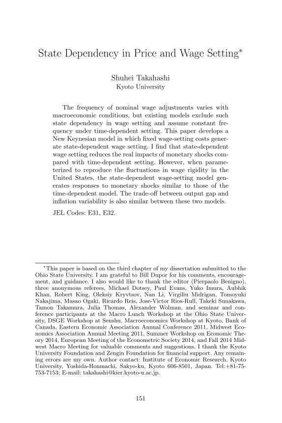
State Dependency in Price and Wage Setting∗
Shuhei TakahashiKyoto University
The frequency of nominal wage adjustments varies withmacroeconomic conditions, but existing models exclude suchstate dependency in wage setting and assume constant fre-quency under time-dependent setting. This paper develops aNew Keynesian model in which fixed wage-setting costs gener-ate state-dependent wage setting. I find that state-dependentwage setting reduces the real impacts of monetary shocks com-pared with time-dependent setting. However, when parame-terized to reproduce the fluctuations in wage rigidity in theUnited States, the state-dependent wage-setting model gen-erates responses to monetary shocks similar to those of thetime-dependent model. The trade-off between output gap andinflation variability is also similar between these two models.
JEL Codes: E31, E32.
∗This paper is based on the third chapter of my dissertation submitted to theOhio State University. I am grateful to Bill Dupor for his comments, encourage-ment, and guidance. I also would like to thank the editor (Pierpaolo Benigno),three anonymous referees, Michael Dotsey, Paul Evans, Yuko Imura, AubhikKhan, Robert King, Oleksiy Kryvtsov, Nan Li, Virgiliu Midrigan, TomoyukiNakajima, Masao Ogaki, Ricardo Reis, Jose-Victor Rios-Rull, Takeki Sunakawa,Tamon Takamura, Julia Thomas, Alexander Wolman, and seminar and con-ference participants at the Macro Lunch Workshop at the Ohio State Univer-sity, DSGE Workshop at Senshu, Macroeconomics Workshop at Kyoto, Bank ofCanada, Eastern Economic Association Annual Conference 2011, Midwest Eco-nomics Association Annual Meeting 2011, Summer Workshop on Economic The-ory 2014, European Meeting of the Econometric Society 2014, and Fall 2014 Mid-west Macro Meeting for valuable comments and suggestions. I thank the KyotoUniversity Foundation and Zengin Foundation for financial support. Any remain-ing errors are my own. Author contact: Institute of Economic Research, KyotoUniversity, Yoshida-Honmachi, Sakyo-ku, Kyoto 606-8501, Japan. Tel:+81-75-753-7153; E-mail: [email protected].
151
152 International Journal of Central Banking February 2017
1. Introduction
The transmission of monetary disturbances has been an importantissue in macroeconomics. Recent studies, such as Huang and Liu(2002) and Christiano, Eichenbaum, and Evans (2005), show thatnominal wage stickiness is one of the key factors in generating per-sistent responses of output and inflation to monetary shocks in NewKeynesian models. However, existing studies establish the impor-tance of sticky wages under Calvo (1983)-style or Taylor (1980)-stylesetting. Such time-dependent setting models are extreme in thatbecause of the exogenous timing and constant frequency of wagesetting, wage adjustments occur only through changes in the inten-sive margin. In contrast, there is some evidence that the extensivemargin also matters, i.e., evidence for state dependency in wage set-ting. For example, reviewing empirical studies on micro-level wageadjustments, Taylor (1999) concludes that “the frequency of wagesetting increases with the average rate of inflation.” Further, accord-ing to Daly, Hobijn, and Lucking (2012) and Daly and Hobijn (2014),the fraction of wages not changed for a year rises in recessions inthe United States.1 How does the impact of monetary shocks differunder state-dependent and time-dependent wage setting? Does statedependency in wage setting significantly affect the monetary trans-mission and the trade-off between output and inflation variability inthe U.S. economy?
To answer these questions, the present paper constructs a NewKeynesian model with state-dependent price and wage setting, build-ing on the seminal state-dependent pricing model of Dotsey, King,and Wolman (1999).2 The price-setting side of the model is essen-tially the same as that of Dotsey, King, and Wolman (1999). Firmschange their price in a staggered manner because fixed costs for price
1In addition to these empirical supports, state-dependent wage-setting modelsare theoretically attractive for policy analysis because the timing and frequencyof wage adjustments could change with policy.
2The framework of Dotsey, King, and Wolman (1999) is widely used foranalyzing aggregate price dynamics. Bakhshi, Kahn, and Rudolf (2007) derivethe New Keynesian Phillips curve for the model. Landry (2009, 2010) developsa two-country model with state-dependent pricing and analyzes exchange ratemovements. Dotsey and King (2005, 2006) analyze the impact of various real-side features on the monetary transmission. Nakov and Thomas (2014) analyzeoptimal monetary policy.
Vol. 13 No. 1 State Dependency in Price and Wage Setting 153
adjustments differ across firms. However, since all firms face theidentical sequence of marginal costs and price-setting costs are inde-pendently distributed over time, adjusting firms set the same priceas in typical time-dependent pricing models, making the price dis-tribution tractable. In contrast, the wage-setting side of the presentmodel departs from the flexible-wage setting of Dotsey, King, andWolman (1999). Specifically, as in Blanchard and Kiyotaki (1987)and Erceg, Henderson, and Levin (2000), households supply a dif-ferentiated labor service and set the wage for their labor. Further,I introduce fixed wage-setting costs that differ across householdsand evolve independently over time.3 Hence, households adjust theirwage in a staggered way. Since adjusting households set the samewage under assumptions commonly made for time-dependent set-ting, the wage distribution is also tractable. Therefore, the presentmodel with state dependency in both price and wage setting can besolved with the method developed by Dotsey, King, and Wolman(1999).
The present paper finds that compared with the time-dependentcounterpart, the state-dependent wage-setting model shows asmaller real impact of monetary shocks.4 Further, these two wage-setting regimes could imply opposite relationships between mone-tary non-neutralities and the elasticity of demand for differentiatedlabor services, which is a key parameter for wage setting. Specifi-cally, non-neutralities could decrease with the elasticity under state-dependent wage setting, while as shown by Huang and Liu (2002),non-neutralities increase under time-dependent setting.
To understand the impact of state dependency in wage settingdescribed above, consider an expansionary monetary shock. In thepresence of nominal rigidity, the aggregate price, consumption, andlabor hours all increase, lowering real wages and raising the marginalrate of substitution of leisure for consumption. Because the timing ofwage adjustments is endogenous, the fraction of households raisingtheir wage increases under state-dependent setting. In contrast, the
3Blanchard and Kiyotaki (1987) also assume fixed wage-setting costs. In con-trast, Kim and Ruge-Murcia (2009) introduce convex wage-adjustment costs.
4Following the convention of the state-dependent pricing literature, the tim-ing and frequency of wage adjustments under time-dependent setting are fixed tothose at the steady state of the state-dependent wage-setting model and hencethey are invariant to shocks.
154 International Journal of Central Banking February 2017
fraction remains unchanged under time-dependent setting. Further,the resetting wage, which is common to all adjusting households,rises more quickly under state-dependent setting than under time-dependent setting. The key to this result is that under monopolisticcompetition, the demand for households’ labor hours increases as theaggregate wage rises relative to their wage. This implies that sincemore households raise their wage, adjusting households find it opti-mal to raise their wage more substantially under state-dependentsetting than under time-dependent setting. In response, firms raisetheir price more quickly. Hence, state-dependent wage setting facil-itates nominal adjustments following monetary disturbances andreduces non-neutralities compared with time-dependent setting.5
The relative wage concern also governs the relationship betweenmonetary non-neutralities and the elasticity of demand for differ-entiated labor. Under a higher elasticity, households’ labor hoursdecrease more elastically as their wage rises relative to the aggregatewage. Hence, when wage setting is time dependent, adjusting house-holds raise their wage less substantially under a higher elasticity.Since the fraction of adjusting households is unchanged, monetarynon-neutralities increase with the elasticity under time-dependentwage setting, as shown by Huang and Liu (2002). This relation-ship could be overturned under state-dependent setting. Under ahigher elasticity, labor hours of non-adjusting households increasemore substantially and therefore more households raise their wage.If this effect is strong enough, adjusting households also set a higherwage when the elasticity is higher. As a result, under state-dependentsetting, nominal wage adjustments could occur more quickly andmonetary non-neutralities could become smaller when the elasticityincreases.
Next, the present paper quantifies the impact of state depen-dency in wage setting on the transmission of monetary shocks andthe trade-off between the output gap and inflation stability for the
5Since adjustment decisions are endogenous under state-dependent setting,adjusting households could shift to those who raise their wage substantially. Inthe present model, those who conduct a large wage increase are those who fixedtheir wage for a long period of time. Such a selection effect is weak in the presentmodel and, as shown later, it is consistent with data.
Vol. 13 No. 1 State Dependency in Price and Wage Setting 155
U.S. economy. For this purpose, I augment my model with cap-ital accumulation, capital adjustment costs, habit formation, andvariable capital utilization because as shown by Christiano, Eichen-baum, and Evans (2005) and Smets and Wouters (2007), these real-side features play a crucial role in the monetary transmission of aNew Keynesian model. Further, several real shocks are introduced inorder to generate a trade-off between stabilizing the output gap andinflation. I then choose the distribution of wage-setting costs so thatthe model reproduces the fluctuations in the fraction of wages notchanged for a year, specifically the variation in the “wage rigiditymeter” released by the Federal Reserve Bank of San Francisco.6
I find that the distribution of wage-setting costs is similar tothe Calvo-type distribution. More specifically, in any given period,most households draw costs close to zero or the maximum, implyingsmall fluctuations in the extensive margin. As a result, the state-dependent wage-setting model shows a response to monetary shocksquite similar to that of the time-dependent counterpart. For exam-ple, the cumulative response of output decreases only by about 10percent when wage setting switches from time to state dependency.The trade-off between the stability of the output gap and the sta-bility of inflation is also similar between the two models, and theoptimal interest rate monetary policy rule under time-dependentwage setting performs well under state-dependent wage setting. Theresults indicate that the time-dependent wage-setting model is agood approximation to the state-dependent wage-setting model con-sidered here and calibrated to the variation in wage rigidity in theUnited States, at least for analyzing the monetary transmission andthe optimal interest rate rule.
This paper is related to the literature that studies how vari-ous features of wage setting influence the transmission of monetaryshocks. Olivei and Tenreyro (2007, 2010) show that the seasonal-ity in the output response to a monetary shock can be explainedby the seasonality in the frequency of wage changes. Dixon and LeBihan (2012) show that considering the heterogeneity in wage spells
6Such long-term rigid wages are key to generating the persistent response tomonetary shocks in New Keynesian models (Dixon and Kara 2010). Further, asdiscussed in footnote 5, the selection effect in the present model mainly worksthrough changes in the fraction of those long-term rigid wages.
156 International Journal of Central Banking February 2017
observed in micro-level data helps account for the persistent responseof output and inflation to a monetary shock. Although these stud-ies analyze important patterns of wage setting, their models assumetime-dependent wage setting. The present paper contributes to theliterature by examining state dependency in wage setting, which isanother feature of wage adjustments.
This paper is also related to the literature on state-dependentprice setting. Following Caplin and Spulber (1987) and Caplinand Leahy (1991), more recent contributions analyze how state-dependent pricing influences the monetary transmission in adynamic stochastic general equilibrium model. Examples includeDotsey, King, and Wolman (1999), Dotsey and King (2005, 2006),Klenow and Kryvtsov (2005, 2008), Devereux and Siu (2007),Golosov and Lucas (2007), Gertler and Leahy (2008), Nakamura andSteinsson (2010), Costain and Nakov (2011a, 2011b), and Midrigan(2011). While these studies describe price setting in a rich way, theyassume flexible wages. The contribution of the present paper is toconstruct a full-blown model with state-dependent price and wagesetting, which is comparable to the state-of-the-art models withtime-dependent price and wage setting developed by Christiano,Eichenbaum, and Evans (2005) and Smets and Wouters (2007).
The rest of the present paper is organized as follows. Section 2describes the benchmark model with state-dependent price and wagesetting, and section 3 determines the parameter values. Section 4uses the benchmark model to show how state dependency in wagesetting influences the transmission of monetary disturbances. Section5 develops the full model with various real-side features and shocksin order to evaluate the importance of state dependency in wage set-ting to the monetary transmission and the trade-off between outputand inflation stability for the U.S. economy. Section 6 concludes.
2. Benchmark Model
This section introduces state dependency in price and wage settinginto a simple New Keynesian model. To this end, I assume fixedcosts for price and wage changes and make the timing of price andwage adjustments endogenous.
Vol. 13 No. 1 State Dependency in Price and Wage Setting 157
2.1 Firms
There is a continuum of firms of measure one.7 Each firm producesa differentiated good indexed by z ∈ [0, 1]. The production functionis
yt(z) = kt(z)1−αnt(z)α, (1)
where α ∈ [0, 1], yt(z) is output, kt(z) is capital, and nt(z) is thecomposite labor, which is defined below. As in Dotsey, King, andWolman (1999) and Erceg, Henderson, and Levin (2000), house-holds own capital, and the total amount of capital is fixed.8 Firmsrent capital and the composite labor in competitive markets. Costminimization implies the following first-order conditions:
αmct
[kt(z)nt(z)
]1−α
= wt (2)
and
(1 − α)mct
[kt(z)nt(z)
]−α
= qt, (3)
where mct is the real marginal cost, wt is the real wage for thecomposite labor, and qt is the real rental rate of capital.
Each firm sets the price of its product Pt(z), and the demand foreach product ct(z) is given by
ct(z) =[Pt(z)Pt
]−εp
ct, (4)
where εp > 1 and Pt is the aggregate price index, which is definedas
Pt =[∫ 1
0Pt(z)1−εp
dz
] 11−εp
, (5)
7This subsection closely follows the explanation by Dotsey, King, and Wolman(1999).
8The full model in section 5 introduces aggregate total factor productivity(TFP) shocks, capital accumulation, and variable capital utilization. I also solvedthe model with no capital (α = 1) and found no significant change relative to theresults of the benchmark model.
158 International Journal of Central Banking February 2017
and ct is the demand for the composite good. The composite goodis defined by
ct =[∫ 1
0ct(z)
εp−1εp dz
] εp
εp−1
. (6)
Firms produce the quantity demanded: yt(z) = ct(z).Firms change their price infrequently because price adjustments
incur fixed costs. Specifically, in each period, each firm draws a fixedprice-setting cost ξp
t (z), denominated in the composite labor, froma continuous distribution Gp(ξp). These costs are independentlyand identically distributed across time and firms. Since firms facethe identical marginal cost of production, the resetting price P ∗
t
is common to all adjusting firms, as under typical time-dependentprice setting. Consequently, at the beginning of any given periodbefore drawing current price-setting costs, firms are distinguishedonly by the last price adjustment and a fraction θp
j,t of firms chargeP ∗
t−j , j = 1, . . . , J . The price distribution, including the number ofprice vintages J, is endogenously determined. Since inflation is pos-itive and price-setting costs are bounded, firms eventually changetheir price and J is finite.
Let vp0,t denote the real value of a firm that resets its price in the
current period and vpj,t, j = 1, . . . , J − 1 denote the real value of a
firm that keeps its price unchanged at P ∗t−j . No firm keeps its price
at P ∗t−J . Each firm changes its price if
vp0,t − vp
j,t ≥ wtξpt (z). (7)
The left-hand side is the benefit of changing the price, while theright-hand side is the cost. For each price vintage, the fraction offirms that change their price is given by
αpj,t = Gp
(vp0,t − vp
j,t
wt
), (8)
j = 1, . . . , J − 1, and αpJ,t = 1. This is also the probability of price
adjustments before firms draw their current price-setting cost. Thefraction and probability of price changes increase as the benefit ofprice adjustments increases.
Vol. 13 No. 1 State Dependency in Price and Wage Setting 159
The value of a firm that adjusts its price is
vp0,t = max
P ∗t
{(P ∗
t
Pt− mct
) (P ∗
t
Pt
)−εp
ct (9)
+ βEtλt+1
λt[(1 − αp
1,t+1)vp1,t+1 + αp
1,t+1vp0,t+1 − wt+1Ξ
p1,t+1]
},
where Et is the conditional expectation and λt is households’ mar-ginal utility of consumption. The first line is the current profit. Thesecond line is the present value of the expected profit. With prob-ability (1 − αp
1,t+1), the firm keeps P ∗t in the next period. With
probability αp1,t+1, the firm resets its price again in the next period.
The last term is the expected next-period price-setting cost, andΞp
j,t+1, j = 1, . . . , J is defined by
Ξpj,t+1 =
∫ ξpj,t+1
0xgp(x)dx, (10)
where gp denotes the probability density function of price-settingcosts. Note that ξp
J,t+1 = Bp, where Bp is the maximum cost.The value of a firm that keeps its price is
vpj,t =
(P ∗
t−j
Pt− mct
) (P ∗
t−j
Pt
)−εp
ct + βEtλt+1
λt
×[(1 − αp
j+1,t+1)vpj+1,t+1 + αp
j+1,t+1vp0,t+1 − wt+1Ξ
pj+1,t+1
],
(11)
j = 1, . . . , J − 2, and
vpJ−1,t =
(P ∗
t−(J−1)
Pt− mct
) (P ∗
t−(J−1)
Pt
)−εp
ct
+ βEtλt+1
λt[vp
0,t+1 − wt+1ΞpJ,t+1]. (12)
The optimal resetting price P ∗t satisfies the first-order condition
for (9): (P ∗
t
Pt
)−εp
ct
Pt− εp
(P ∗
t
Pt− mct
) (P ∗
t
Pt
)−εp−1ct
Pt
+ βEtλt+1
λt(1 − αp
1,t+1)∂vp
1,t+1
∂P ∗t
= 0. (13)
160 International Journal of Central Banking February 2017
Replacing the terms ∂vpj,t+j/∂P ∗
t , j = 1, . . . , J −1 with (11) and (12)yields
P ∗t =
εp
εp − 1
Et
∑J−1j=0 βj
(ωp
j,t+j
ωp0,t
) (λt+j
λt
)P εp−1
t+j ct+jPt+jmct+j
Et
∑J−1j=0 βj
(ωp
j,t+j
ωp0,t
) (λt+j
λt
)P εp−1
t+j ct+j
,
(14)
where ωpj,t+j/ωp
0,t = (1 − αpj,t+j)(1 − αp
j−1,t+j−1) · · · (1 − αp1,t+1), j =
1, . . . , J − 1 is the probability of keeping P ∗t until t + j. The prob-
ability is invariant over time under time-dependent setting. In thepresent model, in contrast, the probability endogenously evolves,reflecting state dependency in price setting (see (8)). However, asin typical time-dependent price-setting models, the optimal price isa constant markup times the weighted average of the current andexpected future nominal marginal costs (Pt+jmct+j).
2.2 Households
There is a continuum of households of measure one. Each householdsupplies a differentiated labor service, which is indexed by h ∈ [0, 1].A household’s preferences are represented by
Et
∞∑l=0
βl[ln ct+l(h) − χnt+l(h)ζ ], (15)
where β ∈ (0, 1), χ > 0, ζ ≥ 1, ct(h) is consumption of the compositegood, and nt(h) is hours worked.
Each household sets the wage rate for its labor service Wt(h)and supplies labor hours demanded nt(h). As in Erceg, Henderson,and Levin (2000), a representative labor aggregator combines house-holds’ labor services, and all firms hire the composite labor from theaggregator. The composite labor is defined as
nt =[∫ 1
0nt(h)
εw−1εw dh
] εw
εw−1
, (16)
Vol. 13 No. 1 State Dependency in Price and Wage Setting 161
where εw > 1. Cost minimization by the labor aggregator impliesthe demand for each labor service:
nt(h) =[Wt(h)
Wt
]−εw
nt, (17)
where Wt is the aggregate wage index, which is defined as
Wt =[∫ 1
0Wt(h)1−εw
dh
] 11−εw
. (18)
Households infrequently adjust their wage because wage settingincurs fixed costs. Similar to price setting, in each period, eachhousehold draws a fixed wage-setting cost ξw
t (h), denominated inthe composite labor, from a continuous distribution Gw(ξw). Thesecosts are independently and identically distributed over time andacross households.
As in typical New Keynesian models, there exists a complete setof nominal contingent bonds, implying that a household faces thebudget constraint
qtkt(h) +Wt(h)nt(h)
Pt+
Mt−1(h)Pt
+Bt−1(h)
Pt+
Dt(h)Pt
= ct(h) +δt+1,tBt(h)
Pt+
Mt(h)Pt
+ wtξwt (h)It(h), (19)
where kt(h) is capital holding, Mt(h) is money holding, Bt−1(h)is the quantity of the contingent bond given the current state ofnature, Dt(h) is nominal profits paid by firms, δt+1,t is the vectorof the prices of contingent bonds, Bt(h) is the vector of those bondspurchased, and It(h) is the indicator function that takes one if house-holds reset their wage in the period and zero otherwise. Assumingthat households have identical initial wealth and the utility func-tion is separable between consumption and leisure, households haveidentical consumption as a result of perfect insurance: λt(h) = λt.
9
9As in Khan and Thomas (2014), I assume nominal bonds contingent on bothaggregate and idiosyncratic shocks. Another setting that leads to perfect insur-ance for consumption is a representative household with a large number of work-ers, as in Huang, Liu, and Phaneuf (2004). Relaxing the assumption of perfectconsumption insurance requires keeping track of the joint distribution of wagesand wealth across households. I leave it to future research.
162 International Journal of Central Banking February 2017
The existence of perfect insurance for consumption implies thatthe optimal wage W ∗
t is common to all adjusting households, asunder standard time-dependent setting. Accordingly, at the start ofany given period, a fraction θw
q,t of households charge W ∗t−q, q =
1, . . . , Q. The wage distribution, including the number of wagevintages Q, is endogenously determined. Under positive inflationand bounded wage-setting costs, households eventually change theirwage and Q is finite.
Let vw0,t denote the utility of a household (relating to wage-
setting decisions) that resets its wage in the current period andvwq,t, q = 1, . . . , Q − 1 denote the utility of a household that keeps
its wage unchanged at W ∗t−q. No household keeps its wage at W ∗
t−Q.Each household changes its wage if
vw0,t − vw
q,t ≥ wtλtξwt (h). (20)
The left-hand side is the benefit of changing the wage, while theright-hand side is the cost. For each wage vintage, the fraction ofadjusting households is given by
αwq,t = Gw
(vw0,t − vw
q,t
wtλt
), (21)
q = 1, . . . , Q − 1, and αwQ,t = 1. This is also the probability of wage
adjustments before households draw their current wage-setting cost.The fraction and probability of wage changes increase with the valueof adjusting wages.
The utility of a household adjusting its wage is
vw0,t = max
W ∗t
⎧⎨⎩λt
W ∗t
Pt
(W ∗
t
Wt
)−εw
nt − χ
[(W ∗
t
Wt
)−εw
nt
]ζ
+ βEt[(1 − αw1,t+1)v
w1,t+1 + αw
1,t+1vw0,t+1 − λt+1wt+1Ξw
1,t+1]
⎫⎬⎭ .
(22)
The first line is the current utility. The second line is the presentvalue of the expected utility. With probability (1 − αw
1,t+1), thehousehold keeps W ∗
t in the next period. With probability αw1,t+1,
Vol. 13 No. 1 State Dependency in Price and Wage Setting 163
the household resets its wage again in the next period. The lastterm is the present value of the expected next-period wage-settingcost, and Ξw
q,t+1, q = 1, . . . , Q is defined by
Ξwq,t+1 =
∫ ξwq,t+1
0xgw(x)dx, (23)
where gw denotes the probability density function of wage-settingcosts. Note that ξw
Q,t+1 = Bw, where Bw is the maximum cost.The utility of a non-adjusting household is
vwq,t = λt
W ∗t−q
Pt
(W ∗
t−q
Wt
)−εw
nt − χ
[(W ∗
t−q
Wt
)−εw
nt
]ζ
+ βEt[(1 − αwq+1,t+1)v
wq+1,t+1 + αw
q+1,t+1vw0,t+1
− λt+1wt+1Ξwq+1,t+1], (24)
q = 1, . . . , Q − 2, and
vwQ−1,t
= λt
W ∗t−(Q−1)
Pt
(W ∗
t−(Q−1)
Wt
)−εw
nt − χ
[(W ∗
t−(Q−1)
Wt
)−εw
nt
]ζ
+ βEt[vw0,t+1 − λt+1wt+1Ξw
Q,t+1]. (25)
The optimal wage W ∗t satisfies the first-order condition for (22):
λt
Pt
(W ∗
t
Wt
)−εw
nt − εwλtW ∗
t
Pt
(W ∗
t
Wt
)−εw−1nt
Wt
+ εwχζ
(W ∗
t
Wt
)−εwζ−1nζ
t
Wt
+ βEt(1 − αw1,t+1)
∂vw1,t+1
∂W ∗t
= 0. (26)
164 International Journal of Central Banking February 2017
Replacing the terms ∂vwq,t+q/∂W ∗
t , q = 1, . . . , Q − 1 with (24) and(25) implies that
Et
Q−1∑q=0
βq
(ωw
q,t+q
ωw0,t
)
×
⎧⎨⎩
εw − 1εw
W ∗t
Pt+qλt+q − χζ
[(W ∗
t
Wt+q
)−εw
nt+q
]ζ−1⎫⎬⎭
×(
W ∗t
Wt+q
)−εw
nt+q = 0, (27)
where ωwq,t+q/ωw
0,t = (1 − αwq,t+q)(1 − αw
q−1,t+q+1)...(1 − αw1,t+1), q =
1, . . . , Q − 1 denotes the probability of keeping W ∗t until t + q.
Because of state dependency in wage setting, the probability endoge-nously varies over time, as indicated by (21). However, as undertime-dependent setting, households set the wage equating the dis-counted expected marginal utility of labor income with the dis-counted expected marginal disutility of labor.
2.3 Money Demand
As in Dotsey, King, and Wolman (1999), the money demand functionis given by
lnMt
Pt= ln ct − ηRt, (28)
where Mt is the quantity of money, η ≥ 0, and Rt is the net nominalinterest rate, which is defined by
11 + Rt
= βEt
(λt+1
λt
Pt
Pt+1
)= βEt
(λt+1
λt
1Πt+1
). (29)
Here, Πt+1 is the gross inflation rate.10
10See Dotsey and King (2006) for the rationale for the use of this type of themoney demand function. The money demand function of (28) can be derivedfrom the money-in-the-utility model with a specific utility function, as shown in,for example, Walsh (2010).
Vol. 13 No. 1 State Dependency in Price and Wage Setting 165
3. Parameter Values
The third column of table 1 lists the parameter values for the bench-mark model. The values are similar to those used in previous studies,such as Huang and Liu (2002) and Christiano, Eichenbaum, andEvans (2005). The length of a period is one quarter. The annual realinterest rate is 4 percent and β = 0.99. The exponent of labor ζ is2.0, implying a Frisch labor supply elasticity of 1.0. The compositelabor supplied at the steady state nss is 30 percent of the total timeendowment (normalized to one), which implies χ = 2.46. The elas-ticity of output with labor α is 0.64. The elasticity of demand fordifferentiated goods εp and that for differentiated labor services εw
are 6.0, generating 20 percent markup rates under flexible pricesand wages.11 The interest semi-elasticity of money demand η is4.0, implying that a 1-percentage-point increase in the annualizednominal interest rate leads to a 1 percent reduction in real moneybalances, which is in line with the estimate by Christiano, Eichen-baum, and Evans (2005).12 I assume 3 percent annual inflation atthe steady state, which is close to the average inflation for the lasttwo decades in the United States. Thus, the quarterly steady-stateinflation rate Π and money growth rate μ are 1.030.25.
As for the distribution of price-setting costs, I follow Dotsey,King, and Wolman (1999) in assuming a flexible distributionalfamily:
ξp(x) = Bp arctan(bpx − dpπ) + arctan(dpπ)arctan(bp − dpπ) + arctan(dpπ)
, (30)
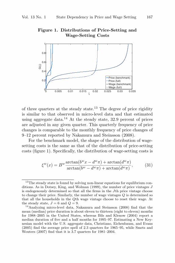
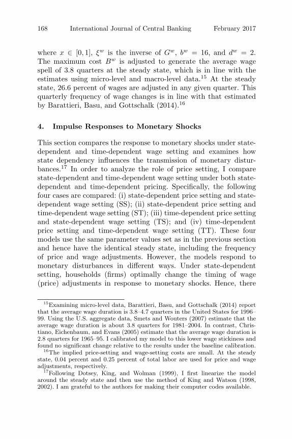
where x ∈ [0, 1] and ξp is the inverse of Gp. For illustrative purposes,the benchmark model uses a shape similar to that assumed by Dot-sey, King, and Wolman (1999) (bp = 16 and dp = 2, figure 1). Themaximum cost Bp is adjusted to produce the average price duration
11Huang and Liu (2002) set εp = 10, whereas Christiano, Eichenbaum, andEvans (2005) estimate εp = 6 in their benchmark model. For εw, Huang and Liu(2002) use 2–6, whereas Christiano, Eichenbaum, and Evans (2005) set it at 21.
12I also solved the model with a higher interest semi-elasticity, η = 17.65, whichis the value used by Dotsey, King, and Wolman (1999). The results did not changesubstantially relative to those under the baseline calibration.
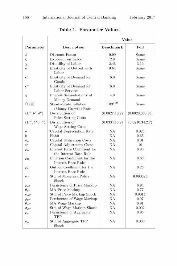
166 International Journal of Central Banking February 2017
Table 1. Parameter Values
Value
Parameter Description Benchmark Full
β Discount Factor 0.99 Sameζ Exponent on Labor 2.0 Sameχ Disutility of Labor 2.46 3.19α Elasticity of Output with
Labor0.64 Same
εp Elasticity of Demand forGoods
6.0 Same
εw Elasticity of Demand forLabor Services
6.0 Same
η Interest Semi-elasticity ofMoney Demand
4.0 Same
Π (μ) Steady-State Inflation(Money Growth) Rate
1.030.25 Same
(Bp, bp, dp) Distribution ofPrice-Setting Costs
(0.0027,16,2) (0.0020,360,35)
(Bw, bw, dw) Distribution ofWage-Setting Costs
(0.0334,16,2) (0.0210,34,2.7)
δ Capital Depreciation Rate NA 0.025b Habit NA 0.65σa Capital Utilization Costs NA 0.01ψ Capital Adjustment Costs NA 10ρR Interest Rate Coefficient for
the Interest Rate RuleNA 0.80
ρΠ Inflation Coefficient for theInterest Rate Rule
NA 0.63
ρy Output Coefficient for theInterest Rate Rule
NA 0.25
σR Std. of Monetary PolicyShock
NA 0.000625
ρμp Persistence of Price Markup NA 0.94θμp MA Price Markup NA 0.77σμp Std. of Price Markup Shock NA 0.0014ρμw Persistence of Wage Markup NA 0.97θμw MA Wage Markup NA 0.91σμw Std. of Wage Markup Shock NA 0.002ρg Persistence of Aggregate
TFPNA 0.95
σg Std. of Aggregate TFPShock
NA 0.006
Vol. 13 No. 1 State Dependency in Price and Wage Setting 167
Figure 1. Distributions of Price-Setting andWage-Setting Costs
0 0.005 0.01 0.015 0.02 0.025 0.03 0.0350
0.2
0.4
0.6
0.8
1
G( ξ
)
ξ
Price (benchmark)Price (full)Wage (benchmark)Wage (full)
of three quarters at the steady state.13 The degree of price rigidityis similar to that observed in micro-level data and that estimatedusing aggregate data.14 At the steady state, 32.9 percent of pricesare adjusted in any given quarter. This quarterly frequency of pricechanges is comparable to the monthly frequency of price changes of9–12 percent reported by Nakamura and Steinsson (2008).
For the benchmark model, the shape of the distribution of wage-setting costs is the same as that of the distribution of price-settingcosts (figure 1). Specifically, the distribution of wage-setting costs is
ξw(x) = Bw arctan(bwx − dwπ) + arctan(dwπ)arctan(bw − dwπ) + arctan(dwπ)
, (31)
13The steady state is found by solving non-linear equations for equilibrium con-ditions. As in Dotsey, King, and Wolman (1999), the number of price vintages Jis endogenously determined so that all the firms in the Jth price vintage chooseto change their price. Similarly, the number of wage vintages Q is determined sothat all the households in the Qth wage vintage choose to reset their wage. Atthe steady state, J = 6 and Q = 9.
14Analyzing micro-level data, Nakamura and Steinsson (2008) find that themean (median) price duration is about eleven to thirteen (eight to eleven) monthsfor 1988–2005 in the United States, whereas Bils and Klenow (2004) report amedian duration of five and a half months for 1995–97. Estimating a New Key-nesian model with the U.S. aggregate data, Christiano, Eichenbaum, and Evans(2005) find the average price spell of 2.3 quarters for 1965–95, while Smets andWouters (2007) find that it is 3.7 quarters for 1981–2004.
168 International Journal of Central Banking February 2017
where x ∈ [0, 1], ξw is the inverse of Gw, bw = 16, and dw = 2.The maximum cost Bw is adjusted to generate the average wagespell of 3.8 quarters at the steady state, which is in line with theestimates using micro-level and macro-level data.15 At the steadystate, 26.6 percent of wages are adjusted in any given quarter. Thisquarterly frequency of wage changes is in line with that estimatedby Barattieri, Basu, and Gottschalk (2014).16
4. Impulse Responses to Monetary Shocks
This section compares the response to monetary shocks under state-dependent and time-dependent wage setting and examines howstate dependency influences the transmission of monetary distur-bances.17 In order to analyze the role of price setting, I comparestate-dependent and time-dependent wage setting under both state-dependent and time-dependent pricing. Specifically, the followingfour cases are compared: (i) state-dependent price setting and state-dependent wage setting (SS); (ii) state-dependent price setting andtime-dependent wage setting (ST); (iii) time-dependent price settingand state-dependent wage setting (TS); and (iv) time-dependentprice setting and time-dependent wage setting (TT). These fourmodels use the same parameter values set as in the previous sectionand hence have the identical steady state, including the frequencyof price and wage adjustments. However, the models respond tomonetary disturbances in different ways. Under state-dependentsetting, households (firms) optimally change the timing of wage(price) adjustments in response to monetary shocks. Hence, there
15Examining micro-level data, Barattieri, Basu, and Gottschalk (2014) reportthat the average wage duration is 3.8–4.7 quarters in the United States for 1996–99. Using the U.S. aggregate data, Smets and Wouters (2007) estimate that theaverage wage duration is about 3.8 quarters for 1981–2004. In contrast, Chris-tiano, Eichenbaum, and Evans (2005) estimate that the average wage duration is2.8 quarters for 1965–95. I calibrated my model to this lower wage stickiness andfound no significant change relative to the results under the baseline calibration.
16The implied price-setting and wage-setting costs are small. At the steadystate, 0.04 percent and 0.25 percent of total labor are used for price and wageadjustments, respectively.
17Following Dotsey, King, and Wolman (1999), I first linearize the modelaround the steady state and then use the method of King and Watson (1998,2002). I am grateful to the authors for making their computer codes available.
Vol. 13 No. 1 State Dependency in Price and Wage Setting 169
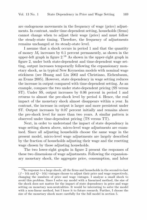
are endogenous movements in the frequency of wage (price) adjust-ments. In contrast, under time-dependent setting, households (firms)cannot change when to adjust their wage (price) and must followthe steady-state timing. Therefore, the frequency of adjustmentsremains unchanged at its steady-state level.
I assume that a shock occurs in period 1 and that the quantityof money Mt increases by 0.1 percent permanently, as shown in theupper-left graph in figure 2.18 As shown in the upper-right graph infigure 2, under both state-dependent and time-dependent wage set-ting, output increases temporarily following the expansionary mon-etary shock, as in typical New Keynesian models with nominal wagestickiness (see Huang and Liu 2002 and Christiano, Eichenbaum,an Evans 2005). However, state dependency in wage setting reducesthe increase in output compared with time-dependent setting. As anexample, compare the two under state-dependent pricing (SS versusST). Under SS, output increases by 0.06 percent in period 1 andreturns to almost the pre-shock level by period 4. Hence, the realimpact of the monetary shock almost disappears within a year. Incontrast, the increase in output is larger and more persistent underST. Output increases by 0.07 percent initially and remains abovethe pre-shock level for more than two years. A similar pattern isobserved under time-dependent pricing (TS versus TT).
Next, in order to understand the impact of state dependency inwage setting shown above, micro-level wage adjustments are exam-ined. Since all adjusting households choose the same wage in thepresent model, micro-level wage adjustments are largely describedby the fraction of households adjusting their wage and the resettingwage chosen by those adjusting households.
The two lower-right graphs in figure 2 present the responses ofthese two dimensions of wage adjustments. Following the expansion-ary monetary shock, the aggregate price, consumption, and labor
18In response to a large shock, all the firms and households in the second-to-last(J −1th and Q−1th) vintages choose to adjust their price and wage respectively,changing the numbers of price and wage vintages. I analyze a small shock toavoid this problem. Since I solve my model with a linearized method, the size ofthe shock does not matter for the impact of state dependency in price and wagesetting on monetary non-neutralities. It would be interesting to solve the modelwith a non-linear method, but I leave it to future research. Further, I choose thesize of the monetary shock more carefully for the full model in section 5.
170 International Journal of Central Banking February 2017
Figure 2. Permanent Increase inMoney—Benchmark Model
2 4 6 8 100
0.05
0.1Output
2 4 6 8 10
0.02
0.04
0.06
0.08
0.1
Aggregate price
2 4 6 8 10
0.02
0.04
0.06
0.08
0.1
Aggregate wage
2 4 6 8 100
0.05
0.1
Money
SS ST TS TT
2 4 6 8 10–0.5
0
0.5
1
Adjusting firms
2 4 6 8 10–0.5
0
0.5
1
Adjusting households
2 4 6 8 100.04
0.06
0.08
0.1
Resetting price
2 4 6 8 100.04
0.06
0.08
0.1
Resetting wage
Notes: The horizontal axis shows quarters. The vertical axis is the percent devi-ation (percentage points deviation for adjusting firms and households) from thesteady state.
Vol. 13 No. 1 State Dependency in Price and Wage Setting 171
hours increase. If households do not raise their wage, their realwage falls, while the marginal rate of substitution of leisure forconsumption rises. Hence, the fraction of households raising theirwage increases under state-dependent setting. For example, underSS, the fraction rises by 0.89 of a percentage point in period 1.In contrast, by construction, the fraction does not increase undertime-dependent setting (ST). Adjusting households also set a higherwage under state-dependent setting than under time-dependent set-ting. The resetting wage rises by 0.084 percent under SS, whereas itrises only by 0.065 percent under ST.
Why does state dependency in wage setting lead to a higherresetting wage? Suppose instead that adjusting households set thesame wage and the resetting wage increases by the same amountunder state-dependent and time-dependent wage setting. Then,since state dependency in wage setting gives a higher number ofadjusting households, the aggregate nominal wage must rise morequickly under state-dependent than under time-dependent setting.The quicker rise in the aggregate wage has two opposing effects onthe optimal resetting wage, as indicated by (27). On one hand, itraises the optimal resetting wage: Because households’ labor hoursincrease with the aggregate wage, as shown in (17), adjusting house-holds need to raise their wage more strongly in order to reduce theirlabor hours. On the other hand, in response to the higher aggregatewage, firms raise their price more quickly. This reduces the increasesin consumption and aggregate labor hours, dampening the rise in theoptimal resetting wage. In addition, since households can choose thetiming of wage adjustments, households under state-dependent wagesetting have less incentive to front-load wage increases than thoseunder time-dependent setting. However, under parameter valuescommonly used in the literature, the relative wage effect dominatesthe other effects. Hence, the resetting wage is higher under state-dependent wage setting than under time-dependent wage setting.
Since more households raise their wage and those households seta higher wage, the aggregate wage rises more quickly and firms alsoraise their price more quickly under state-dependent wage settingthan under time-dependent wage setting. As a result, state depen-dency in wage setting reduces the real impacts of monetary shocks.
The relative wage effect is also the key to the relationshipbetween money non-neutralities and the elasticity of demand for
172 International Journal of Central Banking February 2017
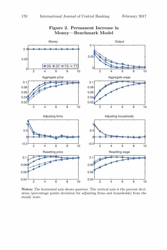
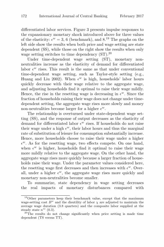
differentiated labor services. Figure 3 presents impulse responses tothe expansionary monetary shock introduced above for three valuesof the elasticity: εw = 3, 6 (benchmark), and 8.19 The graphs on theleft side show the results when both price and wage setting are statedependent (SS), while those on the right show the results when onlywage setting switches to time dependency (ST).20
Under time-dependent wage setting (ST), monetary non-neutralities increase as the elasticity of demand for differentiatedlabor εw rises. This result is the same as that under conventionaltime-dependent wage setting, such as Taylor-style setting (e.g.,Huang and Liu 2002). When εw is high, households’ labor hoursquickly decrease with their wage relative to the aggregate wage,and adjusting households find it optimal to raise their wage mildly.Hence, the rise in the resetting wage is decreasing in εw. Since thefraction of households raising their wage does not change under time-dependent setting, the aggregate wage rises more slowly and moneynon-neutralities become larger for a higher εw.
The relationship is overturned under state-dependent wage set-ting (SS), and the response of output decreases as the elasticity ofdemand for differentiated labor εw rises. If households do not raisetheir wage under a high εw, their labor hours and thus the marginalrate of substitution of leisure for consumption substantially increase.Hence, more households choose to raise their wage under a higherεw. As for the resetting wage, two effects compete. On one hand,when εw is higher, households find it optimal to raise their wagemore mildly relative to the aggregate wage. On the other hand, theaggregate wage rises more quickly because a larger fraction of house-holds raise their wage. Under the parameter values considered here,the resetting wage first decreases and then increases with εw. Over-all, under a higher εw, the aggregate wage rises more quickly andmonetary non-neutralities become smaller.
To summarize, state dependency in wage setting decreasesthe real impacts of monetary disturbances compared with
19Other parameters keep their benchmark value, except that the maximumwage-setting cost Bw and the disutility of labor χ are adjusted to maintain theaverage wage duration (3.8 quarters) and the composite labor supplied at thesteady state nss (0.3).
20The results do not change significantly when price setting is made timedependent (TS versus TT).
Vol. 13 No. 1 State Dependency in Price and Wage Setting 173
Figure 3. Elasticity of Demand for DifferentiatedLabor—Benchmark Model
2 4 6 8 10
0
0.02
0.04
0.06
0.08Output (SS)
3 6 8
2 4 6 8 10
0
0.02
0.04
0.06
0.08Output (ST)
2 4 6 8 100.020.040.060.08
0.1
Aggregate wage (SS)
2 4 6 8 100.020.040.060.08
0.1
Aggregate wage (ST)
2 4 6 8 10
0
0.5
1
Adjusting households (SS)
2 4 6 8 10
0
0.5
1
Adjusting households (ST)
2 4 6 8 100.06
0.08
0.1
Resetting wage (SS)
2 4 6 8 100.06
0.08
0.1
Resetting wage (ST)
Notes: The horizontal axis shows quarters. The vertical axis is the percent devi-ation (percentage points deviation for adjusting firms and households) from thesteady state.
174 International Journal of Central Banking February 2017
time-dependent setting. Further, monetary non-neutralities coulddecrease with the elasticity of demand for differentiated labor ser-vices under state-dependent wage setting, while the opposite rela-tionship holds under time-dependent setting.
5. State Dependency in Wage Settingin the United States
This subsection quantifies the impact of state dependency in wagesetting on monetary non-neutralities and on the trade-off betweenstabilizing the output gap and inflation for the U.S. economy. To thisend, I modify the benchmark model with various real-side featuresand shocks. I then calibrate the distributions of price-setting andwage-setting costs to the patterns of price and wage adjustmentsobserved in the U.S. micro-level data.
5.1 Full Model
The household side is modified as follows. Households’ preferencesinclude habit formation, and the momentary utility function is givenby ln[ct(h) − bct−1(h)] − χnt(h)ζ , where b ∈ [0, 1]. There is capitalaccumulation, and as in Huang and Liu (2002), households choosethe amount of capital that they carry into the next period kt+1(h)subject to quadratic adjustment costs ψ[kt+1(h) − kt(h)]2/kt(h),where ψ > 0. Further, households choose the amount of capitalservices that they supply kt(h) = ut(h)kt(h) by choosing capital uti-lization rate ut(h) subject to costs a(ut(h))kt(h), as in Christiano,Eichenbaum, and Evans (2005). Hence, households face the budgetconstraint:
qtkt(h) +Wt(h)nt(h)
Pt+
Mt−1(h)Pt
+Bt−1(h)
Pt+
Dt(h)Pt
= ct(h) + kt+1(h) − (1 − δ)kt(h) + ψ[kt+1(h) − kt(h)]2
kt(h)
+ a(ut(h))kt(h) +δt+1,tBt(h)
Pt+
Mt(h)Pt
+ wtξwt (h)It(h), (32)
where δ ∈ [0, 1] is the capital depreciation rate. As in Justiniano,Primiceri, and Tambalotti (2010) and Katayama and Kim (2013),
Vol. 13 No. 1 State Dependency in Price and Wage Setting 175
the wage markup rate, μwt ≡ εw
t /(εwt −1), changes stochastically and
follows
lnμwt = (1 − ρμw) lnμw + ρμw lnμw
t−1 + εμw,t − θμwεμw,t−1, (33)
where ρμw ∈ [0, 1), θμw ∈ [0, 1), μw ≡ εw/(εw − 1) is the steady-state wage markup rate, and εμw,t is a wage markup shock that isindependently and identically distributed as N(0, σ2
μw).The firm side of the model is changed as follows. There are shocks
to aggregate total factor productivity (TFP) gt and the productionfunction is
yt(z) = gtkt(z)1−αnt(z)α, (34)
where gt follows an AR(1) process:
ln gt = ρg ln gt−1 + εg,t, (35)
where ρg ∈ [0, 1) and εg,t is a TFP shock that is independently andidentically distributed as N(0, σ2
g). Further, qt in (3) is the real rentalrate of capital services. The price markup rate, μp
t ≡ εpt /(εp
t − 1), issubject to exogenous shocks. Specifically, as in Justiniano, Primiceri,and Tambalotti (2010), it follows that
lnμpt = (1 − ρμp) lnμp + ρμp lnμp
t−1 + εμp,t − θμpεμp,t−1, (36)
where ρμp ∈ [0, 1), θμp ∈ [0, 1), μp ≡ εp/(εp − 1) is the steady-state price markup rate, and εμp,t is a price markup shock thatis independently and identically distributed as N(0, σ2
μp).Lastly, monetary policy is characterized by the interest rate rule
in the spirit of Levin, Wieland, and Williams (1998):
Rt = (1 − ρR)R + ρRRt−1 + ρ lnΠt
Π+ ρy ln
ygt
ygt−1
+ εR,t, (37)
where ρR, ρ, ρy ≥ 0, ygt is the output gap, and εR,t is a mon-
etary shock that is independently and identically distributed asN(0, σ2
R).21
21As in Justiniano, Primiceri, and Tambalotti (2010), the output gap is definedas the deviation of the actual output from the output that would be realized inthe absence of price/wage stickiness and price/wage markup shocks.
176 International Journal of Central Banking February 2017
5.2 Parameter Values
The last column of table 1 lists parameter values for the full model.I first choose the parameter values for the state-dependent price-setting and wage-setting model (SS) and then use the same parame-ter values for the other three models (ST, TS, and TT). The parame-ters appearing in the model of the previous section inherit their orig-inal values, except for the disutility of labor χ, which is adjusted tomaintain the steady-state labor (nss = 0.3), and the parameters onthe distributions of price-setting and wage-setting costs. The capitaldepreciation rate δ is 0.025. I set the habit parameter b = 0.65, whichis the estimate by Christiano, Eichenbaum, and Evans (2005). I alsofollow Christiano, Eichenbaum, and Evans (2005) in setting the cap-ital utilization cost: u = 1, a(1) = 0, and σa = a
′′(1)/a
′(1) = 0.01.
The parameterization generates a peak response of the capital uti-lization rate to a monetary shock that is roughly equal to that ofoutput, which is in line with their finding. Further, I set the capitaladjustment cost parameter ψ = 10 so that, as in Dotsey and King(2006), the peak response of investment to a monetary shock is a bitlarger than twice that of output, which is also consistent with theresults in Christiano, Eichenbaum, and Evans (2005).
For the baseline coefficients of the interest rate policy rule of(37), I use the values estimated by Levin, Wieland, and Williams(1998) for the U.S. economy: ρR = 0.80, ρ = 0.63, and ρy = 0.25.22
I set σR = 0.000625 so that a one-standard-deviation monetary pol-icy shock corresponds to a 25-basis-point change in the annualizedinterest rate, as in Gornemann, Kuester, and Nakajima (2014).23
For the price and wage markup processes, I use the values estimatedby Justiniano, Primiceri, and Tambalotti (2010): ρμp = 0.94, θμp =0.77, σμp = 0.0014, ρμw = 0.97, θμw = 0.91, and σμw = 0.002. Forthe aggregate TFP process, I use the conventional value for persis-tence (ρg = 0.95) and then adjust the volatility σg so that my SSmodel reproduces the volatility of (HP-filtered) output in the U.S.
22See equation (1) of Levin, Wieland, and Williams (1998). The output coeffi-cient is divided by four since the estimated equation is based on the annualizedinterest rate.
23The results of the present section are robust to the size of σR. For example,even when σR doubles, they did not change substantially.
Vol. 13 No. 1 State Dependency in Price and Wage Setting 177
Table 2. Calibration of the Distribution ofWage-Setting Costs
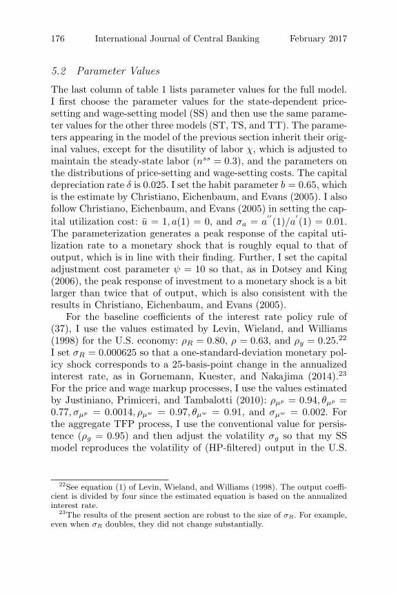
U.S. Data Model
Average Wage Spell (Quarters) 3.8 4.0Fraction of Wages Not Changed for a Year (%) 25 23σfraction/σy 4.5 4.5
data (1.7 percent). The result is σg = 0.006, which is close to theconventional value used in Cooley and Prescott (1995) and others.
I use the distribution of price-setting costs similar to that usedby Klenow and Kryvtsov (2005, 2008). They find that the volatilityof the U.S. inflation is mostly driven by the volatility of the aver-age price change and the volatility of the fraction of price changesplays a minor role. This finding indicates that the distribution ofprice-setting costs must be similar to the Calvo-type distributionunder which almost all firms draw either zero or the maximum price-setting costs. In addition to this, I target an average price spell of3.0 quarters and a quarterly frequency of price adjustments of about33 percent at the steady state. These two targets are motivated bythe estimates by Nakamura and Steinsson (2008). Figure 1 showsthe selected distribution.24
The distribution of wage-setting costs is chosen targeting thethree statistics on micro-level wage adjustments shown in table2. First, the average wage duration is 3.8 quarters at the steadystate, which is consistent with the finding of Barattieri, Basu, andGottschalk (2014) and close to the conventional estimate (see Tay-lor 1999). The other two targets involve the fraction of wages notchanged for a year. I focus on this variable because wage data are
24In contrast, Costain and Nakov (2011a, 2011b) choose the distribution ofprice-setting costs by targeting the empirical size distribution of price changes.Since there are a large number of small price changes, the selected distribution isconcave, which implies that most firms draw a relatively small menu cost. See alsoNakov and Thomas (2014). I solved my model with a similar concave distributionof price-setting costs. Compared with the distribution used here, which essentiallyshuts down state dependency in price setting, monetary non-neutralities becomesmaller. However, the impact of state dependency in wage setting on monetarynon-neutralities is largely unchanged.
178 International Journal of Central Banking February 2017
typically collected annually and most available evidence for statedependency in wage setting is about the fraction of those long-termrigid wages.25 Hence, the second target is the long-run average frac-tion of wages not changed for a year. I target 25 percent based onthe estimate by Barattieri, Basu, and Gottschalk (2014).26
The third target is the volatility of the fraction of wages notchanged for a year. I compute the actual volatility using the wagerigidity meter of the Federal Reserve Bank of San Francisco between1997:Q3 and 2013:Q4. The meter is released monthly and I take thenumber of the middle month of a quarter as the quarterly number.The log of the series is taken and detrended using the Hodrick-Prescott filter of a smoothing parameter of 1,600. The resultingvolatility is 4.5 times as large as the output volatility.27
As figure 1 shows, the distribution is similar to the Calvo-typedistribution in that a large number of households draw either smallor large costs. However, there are some households drawing inter-mediate costs and their adjustment decisions vary with economicstates, generating some state dependency in wage setting. Accord-ingly, as table 2 shows, the calibrated model reasonably reproducesthe data moments.28 In contrast, if the distribution of the bench-mark model is assumed, then the fraction of wages not changed fora year shows a counterfactually high volatility (16.8). If the shape ofthe distribution of price-setting costs is assumed, then the volatilitybecomes too low (0.2) compared with the data value.
25An example is Card and Hyslop (1997). For the United States, a notableexception is Barattieri, Basu, and Gottschalk (2014), who compute the quar-terly frequency of wage adjustments. However, their data cover a relatively shortperiod (1996–99), and it is difficult to compute the volatility of the quarterlyfrequency of wage adjustments.
26The wage rigidity meter released by the Federal Reserve Bank of San Fran-cisco implies a lower fraction: It is about 13 percent between August 1997 andDecember 2013. Given the average wage duration of about a year, it is hard toreproduce this in the model. Hence, I target the finding of Barattieri, Basu, andGottschalk (2014).
27The data are discontinuous in 1997:Q2. While the data for all workers areused here, the volatility does not change very significantly when computed sep-arately for hourly and non-hourly workers (4.3 for hourly workers and 6.0 fornon-hourly workers).
28The wage rigidity meter is the twelve-month moving average of the fractionof wages not changed for a year. Therefore, I take the five-quarter moving averagefor the model statistic to maintain the comparability.
Vol. 13 No. 1 State Dependency in Price and Wage Setting 179
5.3 Impulse Responses to Monetary Policy Shocks
As in the benchmark model, the four price-setting and wage-settingmodels are compared: SS, ST, TS, and TT. These four models havethe identical steady state, including the steady-state frequency ofprice and wage adjustments. However, they respond to monetarydisturbances in different ways.
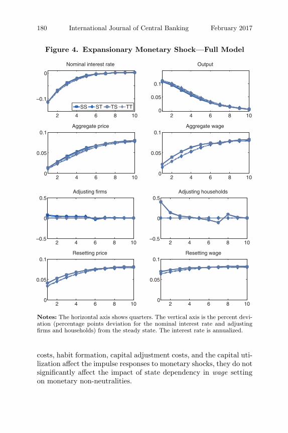
Figure 4 presents the response to an expansionary monetaryshock of one standard deviation (σR = 0.000625) or a negative shockof 25 basis points to the interest rate. As shown, the state-dependentand time-dependent wage-setting models generate quite similarresponses. Although state dependency in wage setting reduces mon-etary non-neutralities, the impact is mild. For example, the cumu-lative response of output for ten quarters after the shock decreasesonly by 9 percent as wage setting switches from time to state depen-dency under state-dependent pricing (SS versus ST). Given theweak state dependency in wage setting, monetary non-neutralitiesincrease with the elasticity of demand for differentiated labor understate-dependent wage setting, as under time-dependent wage setting.Other real and nominal aggregate variables also move in a similarway under state-dependent and time-dependent wage setting.29
As for micro-level wage adjustments, the fraction of adjustinghouseholds increases by around 0.40 percentage point at the onsetof the shock under state-dependent price and wage setting (SS). Theincrease is small relative to the increase in output of 0.11 percent.30
Because of the small increase in the extensive margin, the resettingwage is also only slightly higher under state-dependent wage settingthan under time-dependent wage setting. As a result, the rises inthe aggregate wage are similar between the two wage-setting cases.
What is responsible for the moderate impact of state depen-dency in wage setting? The answer is the distribution of wage-settingcosts. If the distribution of the full model is used for the benchmarkmodel of the previous section, then state dependency in wage settingreduces monetary non-neutralities only by 12 percent, which is sim-ilar to that in the full model. While the distribution of price-setting
29These results are available upon request.30In the benchmark SS model, the fraction of adjusting households initially
increases by 0.90 percentage points, while output increases by 0.06 percent.
180 International Journal of Central Banking February 2017
Figure 4. Expansionary Monetary Shock—Full Model
2 4 6 8 100
0.05
0.1
Output
2 4 6 8 100
0.05
0.1Aggregate price
2 4 6 8 100
0.05
0.1Aggregate wage
2 4 6 8 10
–0.1
0
Nominal interest rate
SS ST TS TT
2 4 6 8 10–0.5
0
0.5Adjusting firms
2 4 6 8 10–0.5
0
0.5Adjusting households
2 4 6 8 100
0.05
0.1Resetting price
2 4 6 8 100
0.05
0.1Resetting wage
Notes: The horizontal axis shows quarters. The vertical axis is the percent devi-ation (percentage points deviation for the nominal interest rate and adjustingfirms and households) from the steady state. The interest rate is annualized.
costs, habit formation, capital adjustment costs, and the capital uti-lization affect the impulse responses to monetary shocks, they do notsignificantly affect the impact of state dependency in wage settingon monetary non-neutralities.
Vol. 13 No. 1 State Dependency in Price and Wage Setting 181
The results of this subsection imply that when calibrated to thevariation in the wage rigidity in the data, the state dependency inwage setting considered here has a minor impact on the response tomonetary disturbances in the United States and the time-dependentwage-setting models approximate the state-dependent models rea-sonably well.
5.4 Trade-off between Output and Inflation Stabilization
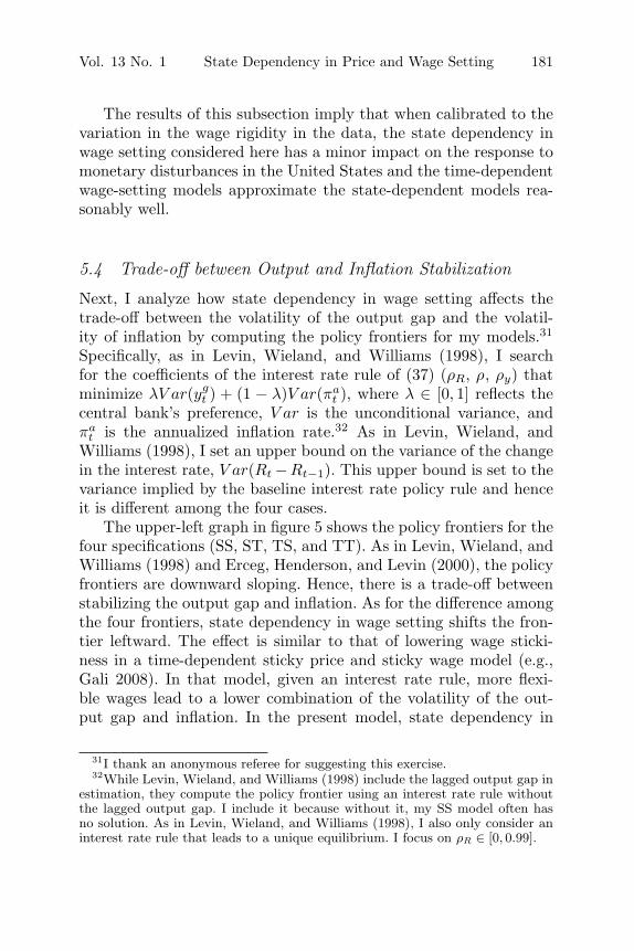
Next, I analyze how state dependency in wage setting affects thetrade-off between the volatility of the output gap and the volatil-ity of inflation by computing the policy frontiers for my models.31
Specifically, as in Levin, Wieland, and Williams (1998), I searchfor the coefficients of the interest rate rule of (37) (ρR, ρ, ρy) thatminimize λV ar(yg
t ) + (1 − λ)V ar(πat ), where λ ∈ [0, 1] reflects the
central bank’s preference, V ar is the unconditional variance, andπa
t is the annualized inflation rate.32 As in Levin, Wieland, andWilliams (1998), I set an upper bound on the variance of the changein the interest rate, V ar(Rt −Rt−1). This upper bound is set to thevariance implied by the baseline interest rate policy rule and henceit is different among the four cases.
The upper-left graph in figure 5 shows the policy frontiers for thefour specifications (SS, ST, TS, and TT). As in Levin, Wieland, andWilliams (1998) and Erceg, Henderson, and Levin (2000), the policyfrontiers are downward sloping. Hence, there is a trade-off betweenstabilizing the output gap and inflation. As for the difference amongthe four frontiers, state dependency in wage setting shifts the fron-tier leftward. The effect is similar to that of lowering wage sticki-ness in a time-dependent sticky price and sticky wage model (e.g.,Gali 2008). In that model, given an interest rate rule, more flexi-ble wages lead to a lower combination of the volatility of the out-put gap and inflation. In the present model, state dependency in
31I thank an anonymous referee for suggesting this exercise.32While Levin, Wieland, and Williams (1998) include the lagged output gap in
estimation, they compute the policy frontier using an interest rate rule withoutthe lagged output gap. I include it because without it, my SS model often hasno solution. As in Levin, Wieland, and Williams (1998), I also only consider aninterest rate rule that leads to a unique equilibrium. I focus on ρR ∈ [0, 0.99].
182 International Journal of Central Banking February 2017
Figure 5. Policy Frontiers and the Coefficients of theOptimal Interest Rate Rule
0.6 0.8 1 1.20.5
1
1.5Policy frontier
std(πa)
y(dtsg)
0.6 0.8 1 1.20
1
2Inflation
std(πa)
tneiciffeoc
0.6 0.8 1 1.20
20
40
60Output gap
std(πa)
tneiciffeoc
0.6 0.8 1 1.20
0.5
1
Lagged interest rate
std(πa)
tneiciffeoc
SS ST TS TT
wage setting essentially makes wage adjustments more flexible com-pared with time-dependent setting. The effect of state-dependentpricing in the present model is also similar to that of lowering pricestickiness in a typical time-dependent model: More price flexibil-ity increases the variance of inflation, shifting the policy frontierrightward.
The remaining graphs in figure 5 show the coefficients of theinterest rate rule against the inflation volatility. In all of the fourcases, it is optimal to smooth the interest rate strongly and respondto both the output gap and inflation. Analyzing various models,Levin, Wieland, and Williams (1998) find that those are robust fea-tures of the optimal interest rate rule. The finding here indicates thattheir conclusion holds for the present model both with and withoutstate dependency in price and wage setting.
Next, I examine the robustness of the optimal interest rate ruleto price-setting and wage-setting specifications, conducting an exer-cise similar to that in section 6 of Levin, Wieland, and Williams(1998). Specifically, I take the optimal policies for λ = 0.25 and 0.75in TT and call them policies A and B, respectively. I then computetwo policy frontiers for each of the four models (SS, ST, TS, and
Vol. 13 No. 1 State Dependency in Price and Wage Setting 183
Figure 6. Robustness of the Interest Rate Rule
0.7 0.8 0.9 1 1.10.5
1
1.5SS
std(πa)
y(dtsg)
A B
0.8 0.9 1 1.1 1.20.5
1
1.5ST
std(πa)
y(dtsg)
A B
0.5 0.6 0.7 0.8 0.90.5
1
1.5TS
std(πa)
y(dtsg)
A B
0.6 0.8 10.5
1
1.5TT
std(πa)
y(dtsg)
A B
TT), setting the upper bound of the variance of the change in theinterest rate to that implied by policies A and B.33
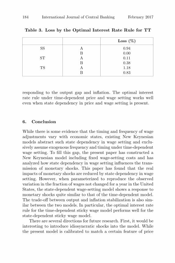
Figure 6 shows the results. The squares indicate the output-inflation volatility under policies A and B. In all the models, thevolatility of the output gap and inflation implied by policies A andB are very close to the respective policy frontiers, suggesting thatpolicies A and B perform well for all of the models.34 As table 3shows, policies A and B incur a small loss relative to the optimalrule even for the models with state dependency in price and wagesetting.
The results of this subsection suggest that the trade-off betweenthe output and inflation volatility and hence implications formonetary policy are quite similar among different price-setting andwage-setting specifications. In all the cases considered, the optimalinterest rate rule is characterized by smoothing the interest rate and
33I take the optimal rules for TT as the benchmark because previous studiestypically analyze an interest rate policy rule under time-dependent sticky pricesand sticky wages.
34For TT, the two policy frontiers coincide because the volatility of a changein the interest rate is the same under policies A and B. Further, the squares areon the policy frontiers.
184 International Journal of Central Banking February 2017
Table 3. Loss by the Optimal Interest Rate Rule for TT
Loss (%)
SS A 0.94B 0.00
ST A 0.11B 0.38
TS A 1.18B 0.83
responding to the output gap and inflation. The optimal interestrate rule under time-dependent price and wage setting works welleven when state dependency in price and wage setting is present.
6. Conclusion
While there is some evidence that the timing and frequency of wageadjustments vary with economic states, existing New Keynesianmodels abstract such state dependency in wage setting and exclu-sively assume exogenous frequency and timing under time-dependentwage setting. To fill this gap, the present paper has constructed aNew Keynesian model including fixed wage-setting costs and hasanalyzed how state dependency in wage setting influences the trans-mission of monetary shocks. This paper has found that the realimpacts of monetary shocks are reduced by state dependency in wagesetting. However, when parameterized to reproduce the observedvariation in the fraction of wages not changed for a year in the UnitedStates, the state-dependent wage-setting model shows a response tomonetary shocks quite similar to that of the time-dependent model.The trade-off between output and inflation stabilization is also sim-ilar between the two models. In particular, the optimal interest raterule for the time-dependent sticky wage model performs well for thestate-dependent sticky wage model.
There are several directions for future research. First, it would beinteresting to introduce idiosyncratic shocks into the model. Whilethe present model is calibrated to match a certain feature of price
Vol. 13 No. 1 State Dependency in Price and Wage Setting 185
and wage setting, in the absence of idiosyncratic shocks, it can-not reproduce some other features observed in the actual data.35
Hence, an important remaining task is to examine the robustnessof the results of the present paper using a model with idiosyncraticshocks. Second, it would be interesting to evaluate the importanceof state dependency in wage setting for countries other than theUnited States. In particular, there are a large number of studies onmicro-level wage adjustments in European countries, and the presentmodel can be calibrated to their findings.36 Third, the present modelis a natural framework to consider optimal monetary policy beyonda simple interest rate rule. In particular, since Nakov and Thomas(2014) analyze optimal monetary policy under state-dependent pric-ing, it would be interesting to examine how their results changeunder state dependency in both price and wage setting. Lastly, state-dependent wage setting could be analyzed in other labor-marketmodels than that analyzed here, such as models with efficiency wagesand labor search and matching.37
References
Bakhshi, H., H. Kahn, and B. Rudolf. 2007. “The Phillips Curveunder State-Dependent Pricing.” Journal of Monetary Econom-ics 54 (8): 2321–45.
Barattieri, A., S. Basu, and P. Gottschalk. 2014. “Some Evidence onthe Importance of Sticky Wages.” American Economic Journal:Macroeconomics 6 (1): 70–101.
Bils, M., and P. J. Klenow. 2004. “Some Evidence on the Importanceof Sticky Prices.” Journal of Political Economy 112 (5): 947–85.
Blanchard, O. J., and N. Kiyotaki. 1987. “Monopolistic Competi-tion and the Effects of Aggregate Demand.” American EconomicReview 77 (4): 647–66.
35For example, there are only price and wage increases in the present model,while price and wage cuts are frequently observed in the actual data.
36Some examples are Fabiani et al. (2010), Walque et al. (2010), and Le Bihan,Montornes, and Heckel (2012).
37Cajner (2011) analyzes state-dependent wage setting in a model with laborsearch and matching.
186 International Journal of Central Banking February 2017
Cajner, T. 2011. “Labor Market Frictions and Bargaining Costs: AModel of State-Dependent Wage Setting.” Mimeo.
Calvo, G. A. 1983. “Staggered Prices in a Utility-Maximizing Frame-work.” Journal of Monetary Economics 12 (3): 383–98.
Caplin, A., and J. Leahy. 1991. “State-Dependent Pricing and theDynamics of Money and Output.” Quarterly Journal of Econom-ics 106 (3): 683–708.
Caplin, A. S., and D. F. Spulber. 1987. “Menu Costs and the Neu-trality of Money.” Quarterly Journal of Economics 102 (4): 703–25.
Card, D., and D. Hyslop. 1997. “Does Inflation ‘Grease the Wheelsof the Labor Market’?” In Reducing Inflation: Motivation andStrategy, ed. C. D. Romer and D. H. Romer 71–114. Chicago:University of Chicago Press.
Christiano, L. J., M. Eichenbaum, and C. L. Evans. 2005. “Nomi-nal Rigidities and the Dynamic Effects of a Shock to MonetaryPolicy.” Journal of Political Economy 113 (1): 1–45.
Cooley, T. F., and E. C. Prescott. 1995. “Economic Growth andBusiness Cycles.” In Frontiers of Business Cycle Research, ed.T. F. Cooley. Princeton, NJ: Princeton University Press.
Costain, J., and A. Nakov. 2011a. “Distributional Dynamics underSmoothly State-Dependent Pricing.” Journal of Monetary Eco-nomics 58 (6–8): 646–65.
———. 2011b. “Price Adjustments in a General Model of State-Dependent Pricing.” Journal of Money, Credit and Banking 43(2–3): 385–406.
Daly, M., and B. Hobijn. 2014. “Downward Nominal Wage RigiditiesBend the Phillips Curve.” Working Paper No. 2013-08, FederalReserve Bank of San Francisco.
Daly, M., B. Hobijn, and B. Lucking. 2012. “Why Has Wage GrowthStayed Strong?” Economic Letter No. 2012-10, Federal ReserveBank of San Francisco.
Devereux, M. B., and H. E. Siu. 2007. “State Dependent Pricing andBusiness Cycle Asymmetries.” International Economic Review48 (1): 281–310.
Dixon, H., and E. Kara. 2010. “Can We Explain Inflation Persis-tence in a Way that Is Consistent with the Microevidence on
Vol. 13 No. 1 State Dependency in Price and Wage Setting 187
Nominal Rigidity?” Journal of Money, Credit and Banking 42(1): 151–70.
Dixon, H., and H. Le Bihan. 2012. “Generalised Taylor and Gener-alised Calvo Price and Wage Setting: Micro-Evidence with MacroImplications.” Economic Journal 122 (May): 532–54.
Dotsey, M., and R. G. King. 2005. “Implications of State-DependentPricing for Dynamic Macroeconomic Models.” Journal of Mon-etary Economics 52 (1): 213–42.
———. 2006. “Pricing, Production, and Persistence.” Journal of theEuropean Economic Association 4 (5): 893–928.
Dotsey, M., R. G. King, and A. L. Wolman. 1999. “State-DependentPricing and the General Equilibrium Dynamics of Money andOutput.” Quarterly Journal of Economics 114 (2): 655–90.
Erceg, C. J., D. W. Henderson, and A. T. Levin. 2000. “OptimalMonetary Policy with Staggered Wage and Price Contracts.”Journal of Monetary Economics 46 (2): 281–313.
Fabiani, S., C. Kwapil, T. Room, K. Galuscak, and A. Lamo. 2010.“Wage Rigidities and Labor Market Adjustment in Europe.”Journal of the European Economic Association 8 (2–3): 497–505.
Gali, J. 2008. Monetary Policy, Inflation, and the Business Cycle.Princeton, NJ: Princeton University Press.
Gertler, M., and J. Leahy. 2008. “A Phillips Curve with an Ss Foun-dation.” Journal of Political Economy 116 (3): 533–72.
Golosov, M., and R. E. Lucas, Jr. 2007. “Menu Costs and PhillipsCurves.” Journal of Political Economy 115 (2): 171–99.
Gornemann, N., K. Kuester, and M. Nakajima. 2014. “Doves forthe Rich, Hawks for the Poor? Distributional Consequences ofMonetary Policy.” Mimeo.
Huang, K. X. D., and Z. Liu. 2002. “Staggered Price-Setting, Stag-gered Wage-Setting, and Business Cycle Persistence.” Journal ofMonetary Economics 49 (2): 405–33.
Huang, K. X. D., Z. Liu, and L. Phaneuf. 2004. “Why Does theCyclical Behavior of Real Wages Change Over Time?” AmericanEconomic Review 94 (4): 836–56.
Justiniano, A., G. E. Primiceri, and A. Tambalotti. 2010. “Invest-ment Shocks and Business Cycles.” Journal of Monetary Eco-nomics 57 (2): 132–45.
188 International Journal of Central Banking February 2017
Katayama, M., and K. H. Kim. 2013. “The Delayed Effects of Mon-etary Shocks in a Two-Sector New Keynesian Model.” Journalof Macroeconomics 38 (Part B): 243–59.
Khan, A., and J. K. Thomas. 2014. “Revisiting the Tale of TwoInterest Rates with Endogenous Asset Market Segmentation.”Review of Economic Dynamics 18 (2): 243–68.
Kim, J., and F. J. Ruge-Murcia. 2009. “How Much Inflation Is Nec-essary to Grease the Wheels?” Journal of Monetary Economics56 (3): 365–77.
King, R. G., and M. W. Watson. 1998. “The Solution of SingularLinear Difference Systems under Rational Expectations.” Inter-national Economic Review 39 (4): 1015–26.
———. 2002. “System Reduction and Solution Algorithms for Sin-gular Linear Difference Systems under Rational Expectations.”Computational Economics 20 (1–2): 57–86.
Klenow, P. J., and O. Kryvtsov. 2005. “State-Dependent or Time-Dependent Pricing: Does It Matter for Recent U.S. Inflation?”NBER Working Paper No. 11043.
———. 2008. “State-Dependent or Time-Dependent Pricing: DoesIt Matter for Recent U.S. Inflation?” Quarterly Journal of Eco-nomics 123 (3): 863–904.
Landry, A. 2009. “Expectations and Exchange Rate Dynamics: AState-Dependent Pricing Approach.” Journal of InternationalEconomics 78 (1): 60–71.
———. 2010. “State-Dependent Pricing, Local-Currency Pric-ing, and Exchange Rate Pass-Through.” Journal of EconomicDynamics and Control 34 (10): 1859–71.
Le Bihan, H., J. Montornes, and T. Heckel. 2012. “Sticky Wages:Evidence from Quarterly Microeconomic Data.” American Eco-nomic Journal: Macroeconomics 4 (3): 1–32.
Levin, A., V. Wieland, and J. C. Williams. 1998. “Robustness ofSimple Monetary Policy Rules under Model Uncertainty.” FEDSPaper No. 45, Board of Governors of the Federal Reserve System.
Midrigan, V. 2011. “Menu Costs, Multiproduct Firms, and Aggre-gate Fluctuations.” Econometrica 79 (4): 1139–80.
Nakamura, E., and J. Steinsson. 2008. “Five Facts about Prices:A Reevaluation of Menu Cost Models.” Quarterly Journal ofEconomics 123 (4): 1415–64.
Vol. 13 No. 1 State Dependency in Price and Wage Setting 189
———. 2010. “Monetary Non-Neutrality in a Multi-Sector MenuCost Model.” Quarterly Journal of Economics 125 (3): 961–1013.
Nakov, A., and C. Thomas. 2014. “Optimal Monetary Policywith State-Dependent Pricing.” International Journal of CentralBanking 10 (3): 49–94.
Olivei, G., and S. Tenreyro. 2007. “The Timing of Monetary PolicyShocks.” American Economic Review 97 (3): 636–63.
———. 2010. “Wage-Setting Patterns and Monetary Policy: Inter-national Evidence.” Journal of Monetary Economics 57 (7): 785–802.
Smets, F., and R. Wouters. 2007. “Shocks and Frictions in US Busi-ness Cycles: A Bayesian DSGE Approach.” American EconomicReview 97 (3): 586–606.
Taylor, J. B. 1980. “Aggregate Dynamics and Staggered Contracts.”Journal of Political Economy 88 (1): 1–23.
———. 1999. “Staggered Price and Wage Setting in Macroeconom-ics.” In Handbook of Macroeconomics, Vol. 1B, ed. J. B. Taylorand M. Woodford, 1009–50 (chapter 15). Elsevier Science B.V.
Walque, G., M. Krause, S. Millard, J. Jimeno, H. L. Bihan, and F.Smets. 2010. “Some Macroeconomic and Monetary Policy Impli-cations of New Micro Evidence on Wage Dynamics.” Journal ofthe European Economic Association 8 (2–3): 506–13.
Walsh, C. E. 2010. Monetary Theory and Policy. MIT Press.