Embed Size (px)
Citation preview
State and Parameter Estimation
in
Quantum Theory
Diplomarbeit
Marcus Kubitzki
AG AudretschFachbereich Physik
Mathematisch-Naturwissenschaftliche SektionUniversitat Konstanz
Juni 2003

Contents
1 Introduction 3
2 Generalized Measurements 5
2.1 Motivation . . . . . . . . . . . . . . . . . . . . . . . . . . . . . . . . . . . . . . . 5
2.2 Mathematical Theory . . . . . . . . . . . . . . . . . . . . . . . . . . . . . . . . . 6
2.2.1 Statistical Analysis of an Experiment . . . . . . . . . . . . . . . . . . . . 7
2.2.2 Hilbert Space Formulation . . . . . . . . . . . . . . . . . . . . . . . . . . . 8
2.3 Physical Realization . . . . . . . . . . . . . . . . . . . . . . . . . . . . . . . . . . 11
2.3.1 Neumark’s Theorem . . . . . . . . . . . . . . . . . . . . . . . . . . . . . . 11
2.3.2 Stern-Gerlach Experiment . . . . . . . . . . . . . . . . . . . . . . . . . . . 12
3 State Estimation 15
3.1 Schemes for Estimating a Pure Quantum State . . . . . . . . . . . . . . . . . . . 16
3.2 Fidelity as Distance Measure for States . . . . . . . . . . . . . . . . . . . . . . . 17
3.3 Disturbance vs. Information Gain in Quantum Operations . . . . . . . . . . . . . 18
3.3.1 Fidelity Balance in Quantum Operations . . . . . . . . . . . . . . . . . . 18
3.3.2 Summary . . . . . . . . . . . . . . . . . . . . . . . . . . . . . . . . . . . . 23
3.4 Optimizing Qubit Measurements . . . . . . . . . . . . . . . . . . . . . . . . . . . 24
3.4.1 Constraint for a Single Measurement . . . . . . . . . . . . . . . . . . . . . 24
3.4.2 Partitioning the FG-Plane . . . . . . . . . . . . . . . . . . . . . . . . . . 25
4 Non-Unitary Operation Partly Reversed by Unitary Means 29
4.1 A Trivial Example . . . . . . . . . . . . . . . . . . . . . . . . . . . . . . . . . . . 29
4.2 Incorporating a Priori Information . . . . . . . . . . . . . . . . . . . . . . . . . . 30
4.2.1 Confining the Integration Volume . . . . . . . . . . . . . . . . . . . . . . . 30
4.2.2 Constructing Us . . . . . . . . . . . . . . . . . . . . . . . . . . . . . . . . 31
4.3 Partial Reversal – Preliminary Results . . . . . . . . . . . . . . . . . . . . . . . . 32
4.3.1 Minimal Term . . . . . . . . . . . . . . . . . . . . . . . . . . . . . . . . . 33
4.3.2 Difference Term . . . . . . . . . . . . . . . . . . . . . . . . . . . . . . . . . 34
4.3.3 First Results . . . . . . . . . . . . . . . . . . . . . . . . . . . . . . . . . . 37
5 Intermezzo: Real-Time Monitoring of Rabi Oscillations 41
5.1 Real-Time Monitoring in a Nutshell . . . . . . . . . . . . . . . . . . . . . . . . . 41
5.2 Single Measurement and N -Series . . . . . . . . . . . . . . . . . . . . . . . . . . . 42
5.2.1 Motivating the Single Measurement E± . . . . . . . . . . . . . . . . . . 42
5.2.2 One N -Series . . . . . . . . . . . . . . . . . . . . . . . . . . . . . . . . . . 44
i
ii CONTENTS
5.3 Best Guess for |c1|2 . . . . . . . . . . . . . . . . . . . . . . . . . . . . . . . . . . . 455.3.1 Motivating gr From Ensembles Using Maximum Likelihood . . . . . . . . 46
5.4 Mean Square Deviation as Measure of Quality . . . . . . . . . . . . . . . . . . . . 475.4.1 Calculating D(gr) . . . . . . . . . . . . . . . . . . . . . . . . . . . . . . . 48
6 Parameter Estimation 516.1 Stating the Problem . . . . . . . . . . . . . . . . . . . . . . . . . . . . . . . . . . 516.2 Revisiting Banaszek: Maximum Likelihood Estimator . . . . . . . . . . . . . . . 52
6.2.1 Estimator for N -Series . . . . . . . . . . . . . . . . . . . . . . . . . . . . . 526.2.2 Mean Square Deviation D(gML) . . . . . . . . . . . . . . . . . . . . . . . . 52
6.3 Incorporating a Priori Information: Bayes’ Theorem . . . . . . . . . . . . . . . . 546.3.1 Prior Information and a Posteriori Distribution . . . . . . . . . . . . . . . 546.3.2 Best Guess, Bayesian Estimator . . . . . . . . . . . . . . . . . . . . . . . . 556.3.3 Implementation to N -Series, Mean Square Deviation D(gBay) . . . . . . . 55
6.4 Comparing all Schemes . . . . . . . . . . . . . . . . . . . . . . . . . . . . . . . . 56
7 Summary and Outlook 617.1 Summary . . . . . . . . . . . . . . . . . . . . . . . . . . . . . . . . . . . . . . . . 617.2 Outlook . . . . . . . . . . . . . . . . . . . . . . . . . . . . . . . . . . . . . . . . . 62
A Calculations in Chapters 3 and 4 63A.1 Inequalities Used for Trade-Off . . . . . . . . . . . . . . . . . . . . . . . . . . . . 63A.2 Calculation of FΩ(Us
√Es) . . . . . . . . . . . . . . . . . . . . . . . . . . . . . . . 64
B Bloch Sphere Representation 67
C Notes on Probability Theory 69C.1 Basics . . . . . . . . . . . . . . . . . . . . . . . . . . . . . . . . . . . . . . . . . . 69C.2 Properties of Estimators . . . . . . . . . . . . . . . . . . . . . . . . . . . . . . . . 70
Zusammenfassung
Diese Arbeit beschaftigt sich mit der Schatzung von Parametern und Zustanden in der Quan-tentheorie. Die Theorie verallgemeinerter Quantenmessungen, vorgestellt in Kapitel 2, bildethierzu den begrifflichen Rahmen.
Der erste Teil der Arbeit, Kapitel 3 und 4 umfassend, untersucht die Balance zwischen derdurch Messung gewonnenen Information und der hierdurch am System verursachten Storung.Fur Einzelmessungen an einem einzigen System wird dieser qualitative Kompromiß quantita-tiv in Form der Fidelities F und G untersucht, insbesondere fur Qubits und Messung selbigervermittels der Klasse unscharfer Messungen. Sie bestehen aus kommutierenden Effekten undkonnen als ‘verschmierte’ Versionen gewohnlicher hermitescher Observablen, wie z.B. Energieoder Spin, interpretiert werden. Es wird gezeigt, daß die optimale Balance zwischen Infor-mationsgewinn und Storung eine einfache Nebenbedingung an die Parameter liefert, die dieseunscharfen Qubit-Messungen charakterisieren.
Die FG-Ebene liefert eine anschauliche Darstellung der Fidelity-Balance. Fur Qubits kannsie ausgedruckt werden durch jene Parameter, die die unscharfe Qubit-Messung reprasentieren.Diese Parametrisierung enthullt eine einfache Struktur, die minimale von nicht-minimalen Mes-sungen trennt (Kraus Operatoren nicht-minimaler Messungen enthalten einen nicht-trivialenunitaren Anteil in ihrer polaren Zerlegung). Es zeigt sich, daß nicht-minimale Messungen dieoptimale Fidelity-Balance deutlich verschlechtern.
Ist vor einer Messung nichts uber den zu schatzenden reinen Qubit-Zustand bekannt, kanneine unitare ‘back-action’, d.h. eine nicht-minimale Messung, die Fidelity F nicht erhohen. Ex-istiert nun aber Vorinformation uber den Zustand, dann verbessert – wie in Kapitel 4 gezeigt wird– diese Information zusammen mit einer passend gewahlten ‘back-action’ die Fidelity, welchefur minimale Messungen mit Vorinformation berechnet wurde. Letztere kann ihrerseits großeroder kleiner sein als die Fidelity, berechnet fur den Fall daß keine Vorinformation uber dasQubit existiert; Information bedeutet nicht unbedingt eine hohere Fidelity. Interessanterweisekann die Fidelity unter Einbeziehung von Vorinformation und diesen speziellen nicht-minimalenMessungen hoher ausfallen als die Fidelity ohne Vorinformation.
Im zweiten Teil der Arbeit, bestehend aus den Kapiteln 5 und 6, verschiebt sich der Schwer-punkt auf die Schatzung von Parametern, die die Dynamik eines Qubits charakterisieren. Auf-bauend auf fuheren Arbeiten [Aud01, Aud02c] zur Echtzeit-Visualisierung von Rabi-Oszillationenmittels Sequenzen unscharfer Messungen (N -Serien), werden verschiedene Schatzverfahren furden Parameter |c1|2 entwickelt und verglichen. Die ursprunglich vorgeschlagene Schatzung[Aud01] wurde im Hinblick auf Erwartungstreue konstruiert, ein Kriterium aus der klassis-chen Schatztheorie. Ein zweites Verfahren wird mit Hilfe der ‘maximum likelihood’-Methodeabgeleitet. Diese Schatzung macht jedoch keinerlei Gebrauch von eventuell vorhandener Vorin-formation uber den Qubit-Zustand. Das dritte Schatzverfahren (‘Bayesian estimator’) bezieht
1
2 CONTENTS
solche Informationen uber den Satz von Bayes mit ein. Um alle Schatzungen vergleichen zukonnen, wird ein mittleres Fehlerquadrat konstruiert um ein Gutemaß zu erhalten. Mit Hilfedieses Maßes kann gezeigt werden, daß fur eine N -Serie das Schatzverfahren von Bayes sowohldem ‘maximum likelihood’- als auch dem ursprunglichen Verfahren uberlegen ist. Letzteres istseinerseits dem ‘maximum likelihood’-Verfahren unterlegen, d.h. die ursprungliche Schatzunghat ein großeres mittleres Fehlerquadrat.
Chapter 1
Introduction
Roughly 25 years ago, physicists began to realize that quantum mechanical systems could beemployed to accomplish information processing tasks beyond classical limitations. Since then,quantum information theory became an ever growing field, boosted by theoretical breakthroughsas well as the steadily increasing ability to control single quantum systems.
Two elementary processes are of great importance to quantum information and quantumcomputation: state estimation and the characterization of the dynamics of a quantum system.This thesis is dealing with both of these aspects, whose applications range from assessing theperformance of quantum gates or quantum communication channels, to the determination oftypes and magnitudes of different noise processes in a system. In each case, information abouta quantum state is necessary, which means that measurements have to be made.
Projective measurements are often useless in this respect, especially when superpositions ofstates occur. Hereby, generalized measurements provide a tool better suited. This concept ofmeasurement, originating in the late 1980s, became the new paradigm of quantum measurementtheory [Bus95, Bus91, Hol82, Kra83], superseding the old formulation of von Neumann which isincluded in this approach.
The mathematical notion of observables as positive operator valued measures (POVMs) –instead of hermitian operators with a projective valued measure (PVM) – had manifold moti-vations, ranging from practical issues to foundational interests in quantum theory. Due to theirexperimental realization as indirect projection measurements, the disturbing influence of gener-alized measurements on a state can be chosen according to special requirements. This featurepredestines them for state estimation and monitoring of dynamics.
As aforementioned, both state estimation and the characterization of dynamics are discussedin this work which consists of two parts: In the first part, the relation between information gainand disturbance is discussed. Emphasis is put on qubits, the simplest non-trivial quantum sys-tem, and the special class of unsharp measurements. The second part is concerned with thecharacterization of dynamics. Rabi oscillations of a qubit provide an exactly solvable modelsystem for studying the real-time visualization of dynamics. Here, different methods for theestimation of parameters characterizing this dynamical behavior can be tested.
This work is structured as follows: Chapter 2 introduces the language of generalized measure-ments, the fundamental tool for investigations into quantum state estimation and parameter es-timation theory. After a short motivation the mathematical theory of generalized measurementsin terms of positive operator valued measures is laid out as well as their experimental realization.
3
4 CHAPTER 1. INTRODUCTION
Chapters 3 and 4 are concerned with the influence unsharp measurements have on quantummechanical systems. In chapter 3 the trade-off between information gain and disturbance isthe main item of interest. A quantitative description of these qualitative terms is providedby the well-known concept of fidelity. For one measurement on a single system the optimalfidelity balance is investigated, especially for the class of minimal unsharp measurements of aqubit. Non-minimal qubit measurements are subject of chapter 4. There, the question of apartial reversal of non-unitary operations (i.e. measurements) by means of unitary back-actionis discussed.
Chapters 5 and 6 deal with parameter estimation and the visualization of dynamics, thelatter being subject of chapter 5. There, the real-time monitoring of a qubit’s Rabi oscillationsby means of a sequence of unsharp measurements motivates estimation of the parameter |c1|2.In analogy to the fidelity, a quantitative measure defining the quality of a guess is developed.Chapter 6 exclusively deals with guesses (estimators) for |c1|2 and their evaluation. In additionto the originally proposed estimator of chapter 5, two new estimators are developed, followedby a comparison of all estimators.
Chapter 7 summarizes all results and gives some ideas for further work.Appendices A, B and C contain detailed calculations omitted in chapters 3 and 4, the Bloch
sphere representation of qubits and basic definitions of probability theory and classical estimationtheory, respectively.
Chapter 2
Generalized Measurements
State and parameter estimation in quantum mechanics are connected by the theory of gener-alized measurements, laid out conceptually and mathematically in this chapter. Generalizedmeasurements as a necessary conceptual leap beyond the long accepted formulation of quan-tum measurements given by von Neumann are motivated1 in section 2.1. Following up on this,section 2.2 provides the mathematical implementation in terms of positive operator valued mea-sures on Hilbert space. The physical realization of generalized measurements together with theStern-Gerlach experiment as a prime example is depicted in the concluding section 2.3.
2.1 Motivation
Since its emergence in the late 1920s, quantum theory on Hilbert space has been the basis offruitful and deep research into virtually all branches of physics. There seems to be no instanceof conflict between theoretical predictions and experimental results. In view of this success itis remarkable that a few conceptual problems have resisted any attempted resolution even untilnow. The most prominent of these is known as the ‘measurement problem’: It paraphrases thefact that a superposition of quantum states
∑
i ci|i〉 reduces upon measurement instantaneouslywith probability |ck|2 to the eigenstate |k〉 of the measured observable. This ‘collapse of thewave function’ (or ‘reduction of the state vector’) badgered physicists since the work of Johnvon Neumann on mathematical foundations of quantum theory [vN32], where he introducedquantum observables as self-adjoint operators in Hilbert space and the aforementioned projectionpostulate to describe the reduced quantum states for discrete observables.
For over 40 years this paradigm stood at the heart of quantum measurement theory togetherwith other conceptual shortcomings (like, for example, the possibility of interpreting quantummechanics as a theory of individual systems with definite real properties, or certain limitationson measurability discovered by Wigner. For details, see chapter one of [Bus95]). Some of thesebecame tractable in the 1980s once the probabilistic structure of quantum mechanics was appre-ciated in its full generality. Besides Gleason’s theorem the introduction of observables as positiveoperator valued measures (POVMs) were a crucial step in this development. Interestingly, thelatter discovery was made independently in a variety of rather disparate areas of physics, mo-tivations ranging from foundational interests to fairly practical needs. This wide scope of the
1Here, as well as in subsections 2.2.1 and 2.3.2, we will closely follow [Bus95].
5
6 CHAPTER 2. GENERALIZED MEASUREMENTS
concept of POVMs demonstrates its status as an integral part of the basic structure of quantumtheory.
Now what are those motivations which led to the incorporation of generalized2 measure-ments (represented by POVMs) into the quantum vocabulary? A quite thorough account onthese matters can be found in [Bus95]. Here, only one specific conceptual problem is sketched,followed by a more in-depth analysis of the Stern-Gerlach experiment in subsection 2.3.2 oncethe mathematical formalism is available.
Some puzzles in the foundations of quantum theory appeared in the form of a conflict be-tween familiar classical physical ideas and some ‘strange’ implications of the quantum formalism.In each case the resolution consisted of rephrasing a strict no-go verdict excluding certain sharp(projective) measurements into a positive statement expressing the possibility of unsharp mea-surements subject to some limitations.
One of these no-go verdicts is the non-commutativity of certain pairs of self-adjoint operators,commonly interpreted as the root of the – classically unknown – incommensurability of thecorresponding observables. From the fundamental commutator relation
[Q,P ] = i~
(2.1)
it was argued that measurements of position and momentum are mutually exclusive and can-not be performed together on single systems. Even worse, Heisenberg’s interpretation of theuncertainty relation
∆Q · ∆P ≥ ~
2, (2.2)
being a consequence of (2.1), limits the accuracy of position and momentum measurementsperformed on ensembles of systems prepared in one and the same state; here, ∆Q and ∆P arethe standard deviations of Q and P in some state ρ.
Instead of accepting the mere incommensurability of position and momentum, the pioneersof quantum theory considered various thought experiments (such as the gamma ray microscope)to demonstrate that joint measurements of these complementary observables should be possiblein principle. The crucial idea hereby was that such measurements must not be too accurate, thelimits of precision given by (2.2). While the measurement indeterminacy interpretation of theuncertainty relation is commonly accepted, its tenability was nevertheless long questioned dueto the lacking rigorous incorporation of the idea of inaccurate measurements into the quantumformalism. Thus, a strict inclusion of unsharp measurements represented by positive operatorvalued measures paved the way for a solution and deeper understanding of this and relatedproblems.
2.2 Mathematical Theory
Generalized measurements were motivated in the preceeding section among other things bythe fact that they arise naturally in the theoretical description of many experiments. Nowwe are providing the main ideas behind POVMs in compact form in subsection 2.2.1 using anexperiment as our guide [Bus95]. Subsequently, the mathematical formulation in familiar termsof operators in Hilbert space is given.
2Although generalized measurements are only introduced in the next section we use the term here to pointout the necessity for a theory of measurement going beyond von Neumann.
2.2. MATHEMATICAL THEORY 7
2.2.1 Statistical Analysis of an Experiment
In analyzing the general features of any physical experiment one is able to specify those math-ematical structures that are relevant to the theoretical description of an experiment. Any typeof physical system is characterized by means of a collection of preparation procedures, the ap-plication of which prepare the system in a state ρ. The set of states is not a simplex, thusaccounting for the fact that the same mixed state can be prepared by different mixtures of purestates. Given a system prepared in a state ρ, a measurement can be applied, leading to theregistration of some outcome ωi. For illustrative purposes, we assume a finite3 set of pointerreadings Ω = ω1, . . . , ωn. The very existence of physical experience is due to the fact that oneis able to observe regularities in the event sequences occurring in nature. In particular, physicalexperimentation as sketched above would lose its meaning, were there not a probabilistic con-nection between the occurrence of a registration and the preceeding preparation. Hence, anypair (ρ, ωi) of a state ρ and an outcome ωi should determine a conditional probability p(ωi
∣
∣ρ),
(ρ, ωi) 7→ p(ωi∣
∣ρ) (2.3)
which in a long run of repeated experiments (N trials) is approximated by the relative frequencyN(ωi)/N of the occurrence of the outcome ωi. It should be noted that different preparationprocedures may be statistically equivalent in that they yield the same statistics for all possiblemeasurements. Therefore the states ρ correspond, strictly speaking, to equivalence classes ofpreparation procedures. Similarly, different registration procedures may be statistically equiva-lent in the sense of yielding the same probabilities in every state. This gives rise to the definitionof an observable as an equivalence class of measurements. In fact, the map (2.3) can be viewedin two ways. First, any outcome ωi induces a state functional Ei,
Ei : ρ 7→ Ei(ρ) := p(ωi∣
∣ρ) (2.4)
called an effect. Now the measured observable may be defined as the map assigning to eachoutcome ωi its associated effect:
E : ωi 7→ Ei . (2.5)
According to the second reading of (2.3), any state ρ fixes a probability distribution
pρ : ωi 7→ pρ(ωi) := p(ωi∣
∣ρ) .
In the simple case of a discrete experiment the properties of such a probability measure aresummarized in the positivity (pρ(ωi) ≥ 0) and normalization (
∑
i pρ(ωi) = 1) conditions. Inview of (2.4) the mapping ρ 7→ pρ is defined by the observable E. Since the properties of pρ arenaturally transferred to E, an observable will appropriately be called an effect valued measure.
It is natural to assume that any state functional Ei preserves the convex structure of the setof states, that is, it associates with any mixture of states the corresponding convex combinationof probability. This is taken as a reflection of the statistical independence of a long run ofidentical measurements performed on an ensemble of mutually independent systems. Effects arethus represented as linear functionals on the space of states.
3This assumption is reasonable and will be used throughout the thesis. See also chapter 5.2 for a justification.
8 CHAPTER 2. GENERALIZED MEASUREMENTS
2.2.2 Hilbert Space Formulation
The general statistical analysis sketched above gives a glimpse on the probabilistic structureunderlying generalized measurements. In the following we shall not be concerned4 with a rigorousmathematical treatment of the introduced effect valued measures. Instead we consider how theseoperationally defined objects enter quantum mechanics in terms of operators in Hilbert space.
One preliminary remark: Throughout this thesis we are solely dealing with closed5 quantumsystems of finite dimension and observables with discrete nondegenerate spectra. Hence, there isno need to introduce the general operator-sum formalism whereby trace and non-trace preservingquantum operations are represented. See, for example, chapter 8 of [Nie01].
Generalized Measurement Postulate
From what we have seen in subsection 2.2.1, we can phrase one aim of quantum measurementtheory: Given the initial state of a system, we want to be able to specify the probability of aparticular measurement result and the state of the system immediately after that measurement.Therefore, we can formulate the postulate for generalized measurements:
Postulate 2.1 (measurement). Quantum measurements are described by a collection Msof measurement operators (often called Kraus operators), acting on the Hilbert space H of thesystem being measured. The index s refers to the measurement outcomes that may occur6 in theexperiment. If the state of the system is |ψ〉 (respectively ρ for mixed states) immediately beforethe measurement then the probability that result s occurs is given by
ps = 〈ψ|M †sMs|ψ〉 resp. ps = tr[M †
sMsρ] ; (2.6)
after a measurement with result s, the system’s state is
|ψ′〉 =Ms|ψ〉
√
〈ψ|M †sMs|ψ〉
resp. ρ′ =MsρM
†s
tr[M †sMsρ]
.
The measurement operators satisfy the completeness relation
∑
s
M †sMs =
, (2.7)
expressing the fact that probabilities add up to one.
The novelty of this postulate (compared to the one of von Neumann) lies in the fact thatany set of operators Ms satisfying (2.7) can represent a measurement. In particular, the Ms
do not have to be projectors, MsMs 6= Ms, nor do they need to be hermitian, i.e. no referenceis necessarily made to any observable.
4The omitted theoretical parts are not significant for the understanding of this thesis, where only state changesinflicted by unsharp measurements are important. Answering fundamental questions requires more detailedmathematical background knowledge, an exhaustive account of which can be found e.g. in [Bus95] and [Bus91].
5closed, except for the duration of a measurement which we assume to be arbitrary short.6In general, different Kraus operators Msi can be associated to one specific measurement outcome s, e.g.
ps =P
i〈ψ|M†
siMsi|ψ〉 and |ψ′〉 =
P
iMsi|ψ〉/ps. In this way noise processes are modeled which we neglect
downright.
2.2. MATHEMATICAL THEORY 9
This raises the question what kind of properties these measurements represent. Often, theproperty a certain POVM7 represents can be determined by making reference to some knownsharp observable (i.e. a hermitian observable represented by a projection valued measure (PVM);e.g. energy, spin, angular momentum, etc.). Indeed many POVMs derive from some PVM by acoarse-graining procedure. For example, a POVM associated with the position variable Q arisesif one performs a convolution of the spectral measure with some confidence function [Bus95].We shall refer to such an unsharp observable as a smeared (position) observable (it then becomespossible to associate with a pair of incommensurable sharp observables a new pair of coexistentunsharp observables which are smeared versions of the original ones. Whether two such unsharpobservables are coexistent or not depends on the degree of smearing involved. In the case ofposition and momentum it is precisely the uncertainty relation (2.2) which serves to characterizethe amount of smearing required for their joint measurability).
Terminology
In order to avoid misunderstandings, let me define our terminology: generalized measurementsdenote all possible POVMs. The term ‘observable’ stands synonymous for a generalized observ-able, described by some arbitrary POVM. Unlike generalized, hermitian observables representedby some spectral measure are called sharp or ordinary observables. Smeared (coarse-grained)versions of sharp observables will be named unsharp. There, the spectral measure of the sharpobservable has been convoluted with some confidence function; thus, from a given measurementresult, no reliable conclusion regarding the initial state can be drawn. Unsharp measurementsare often called weak, referring to the influence such a measurement has on a state comparedto projective measurements. However, the unsharpness in question should in general not onlybe taken as an imperfect perception (like a loose pointer of some measurement apparatus) of anunderlying more sharply determined property. On the contrary, this term is also intended to de-scribe possible elements of reality whose preparation and determination are subject to inherentlimitations.
Speaking of sharp observables and spectral measures, we see that projective measurementsare a special case of the above postulate: by setting
Ms = Ps with PrPs = δrsPs ,
the hermitian observable M =∑
s sPs is measured in accordance with von Neumann’s postulate.
POVM
The quantum measurement postulate involves two elements. First, it gives a rule describing themeasurement statistics, that is, the respective probabilities of the different possible measurementoutcomes. Second, it gives a rule describing the post-measurement state of the system. However,for some applications the post-measurement state is of little interest (e.g. in an experiment wherethe system is measured only once, upon conclusion of the experiment), with the main item ofinterest being measurement statistics. If we define the operator
Es := M †sMs , (2.8)
7we will define a POVM more closely in the next paragraph.
10 CHAPTER 2. GENERALIZED MEASUREMENTS
the probability of measuring outcome s is (for a pure state) given from postulate 2.1 by ps =〈ψ|Es|ψ〉, with |ψ〉 being the initial state before the measurement. Thus, the set of operatorsEs is sufficient to determine the measurement statistics and we can restate (2.4) in terms ofoperators:
Definition 2.1 (POVM). A set of operators Es is named a positive operator valued measure(POVM) if and only if the following two conditions are met:
(i) each operator Es is positive ⇔ 〈ϕ|Es|ϕ〉 ≥ 0 ∀ϕ
(ii) the completeness relation∑
sEs =
is obeyed.
The elements of Es are called effects or POVM elements. On its own, a given POVM Esis enough to have complete knowledge of the probabilities of all possible outcomes; measurementstatistics is the only item of interest. If knowledge about the post-measurement state is favored,we have to use definition (2.8) to connect POVM elements Es with measurement operators Ms.
Minimal and Non-Minimal Measurements
Interestingly, this interconnection of POVM elements and Kraus operators is not unequivocal.In analogy to the decomposition of complex numbers z = |z|eiφ into modulus and phase, asimilar decomposition exists for linear operators on vector spaces (for a proof, see e.g. [Nie01]):
Proposition 2.1 (polar decomposition). Let A be a linear operator on a vector space V.Then there exists unitary U and positive operators J and K such that
A = UJ = KU , (2.9)
where the unique positive operators J and K satisfying (2.9) are defined by J :=√A†A and
K :=√AA†. Moreover, if A is invertible then U is unique. The expression A = UJ is called
the left polar decomposition of A, and A = KU the right polar decomposition of A.
Hence, every Kraus operator on H can be written as Ms = Us|Ms|, with unitary Us andpositive operator |Ms|. Plugging this into (2.8) we get8
Es = M †sMs (2.10)
= |Ms|U †sUs|Ms| (2.11)
= |Ms|2
from what follows
|Ms| =√
Es
Ms = Us√
Es . (2.12)
From (2.10)-(2.12) we see that there is exactly one effect corresponding to each Kraus operator,whereas the reverse is not true. To every POVM element Es corresponds an infinite number ofKraus operators; different possible unitary parts, say Us and Us, are canceled in (2.11).
8Every positive operator is hermitian, i.e. |Ms|† = |Ms|.
2.3. PHYSICAL REALIZATION 11
This has important consequences on the interpretation of the interplay between disturbancecaused by a measurement and information gained from it. Every effect Es just determines thepositive part of each Kraus operator,
√Es = |Ms|. On the other hand we need nothing more than
the effects to determine all probabilities for every possible measurement result, see (2.6). Hence,the unavoidable disturbance inherent to every measurement is completely given by the positivepart of each measurement operator. At the same time,
√Es yields all information one can get
with this measurement. Any non-trivial unitary part Us 6=
in Ms does not contribute extrainformation (In general, this unitary rotation of the measured state in H causes an unwantedadditional disturbance. But, as we will see in chapter 4, this unitary operation can lead as wellto an attenuation of disturbance caused by the positive part
√Es). We therefore define:
Definition 2.2 (minimal, non-minimal). A measurement is called minimal if the respectiveKraus operators have a trivial unitary part, i.e. Us =
for all possible measurement outcomes s:
minimal measurement ⇔ Ms = |Ms| =√
Es .
Consequently, non-minimal measurements have a non-trivial unitary part, Us 6=:
non-minimal measurement ⇔ Ms = Us|Ms| = Us√
Es .
For measurements on ensembles (i.e. N identically prepared copies of one state ρ – notto be confused with the meaning ‘ensemble’ has in statistical mechanics, where it denotes aninfinite number of conceptual replicas of one system) this distinction is of no interest becauseeach ensemble member is measured only once so any additional state transformation has noconsequence on measurement statistics whatsoever. For successive measurements on a singlesystem, the above distinction becomes quite important. In this case, the same system is measured(and thus disturbed) again and again. Thereby, unitary parts cause additional transformationsof the measured state. We will encounter this problem again in section 5.2.
2.3 Physical Realization
2.3.1 Neumark’s Theorem
Talking about generalized measurements is all very well, as long as there exists an operationalscheme by which an experimenter in some laboratory can realize such a measurement. Theexistence of this scheme follows from a theorem due to Neumark, which not only ensures thephysical realizability of every possible POVM but at the same time provides the operationalrules necessary to carry out the measurement.
The theorem basically states that every POVM Es on a Hilbert space H can be extendedto a projection valued measure (PVM) Ps in a larger Hilbert space H ⊃ H.
Thus, every generalized measurement on a system S can be realized by coupling it unitarilyto a second system A (ancilla), thereby entangling both. By means of a projection measurementon the ancilla, the desired POVM on the system S is realized. The number of measurable pointerreadings s is given by the dimension of the ancilla A, which can, in principle, be arbitrary.
While it is true that any POVM can be formally reduced to a PVM acting on a larger Hilbertspace, this does not diminish the need for POVMs in the description of physical systems. If onedoes not want to stick to an account of experiments solely in terms of pointer observables, thus
12 CHAPTER 2. GENERALIZED MEASUREMENTS
dealing with phenomena on the level of measuring devices, one has got to perform the Neumarkprojection: It is this step that enables one to speak of the object under investigation and itsmeasured observable.
2.3.2 Stern-Gerlach Experiment
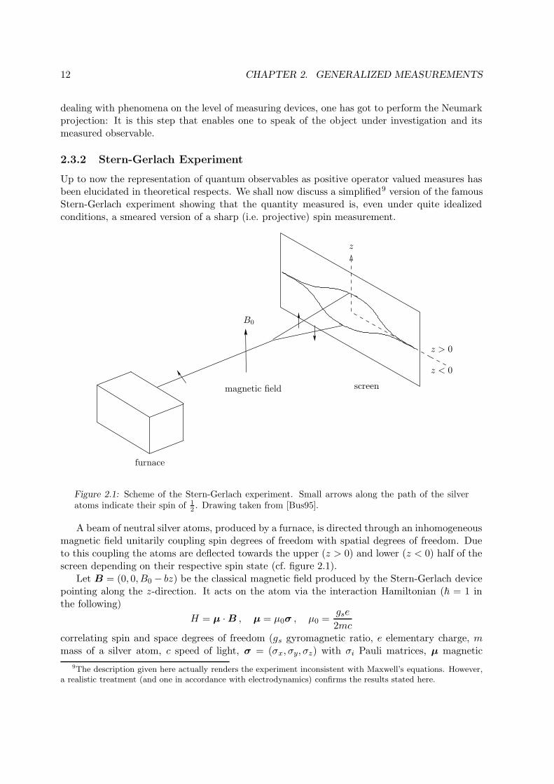
Up to now the representation of quantum observables as positive operator valued measures hasbeen elucidated in theoretical respects. We shall now discuss a simplified9 version of the famousStern-Gerlach experiment showing that the quantity measured is, even under quite idealizedconditions, a smeared version of a sharp (i.e. projective) spin measurement.
furnace
screenmagnetic field
B0
z
z > 0
z < 0
Figure 2.1: Scheme of the Stern-Gerlach experiment. Small arrows along the path of the silveratoms indicate their spin of 1
2. Drawing taken from [Bus95].
A beam of neutral silver atoms, produced by a furnace, is directed through an inhomogeneousmagnetic field unitarily coupling spin degrees of freedom with spatial degrees of freedom. Dueto this coupling the atoms are deflected towards the upper (z > 0) and lower (z < 0) half of thescreen depending on their respective spin state (cf. figure 2.1).
Let B = (0, 0, B0 − bz) be the classical magnetic field produced by the Stern-Gerlach devicepointing along the z-direction. It acts on the atom via the interaction Hamiltonian (~ = 1 inthe following)
H = µ · B , µ = µ0σ , µ0 =gse
2mccorrelating spin and space degrees of freedom (gs gyromagnetic ratio, e elementary charge, mmass of a silver atom, c speed of light, σ = (σx, σy, σz) with σi Pauli matrices, µ magnetic
9The description given here actually renders the experiment inconsistent with Maxwell’s equations. However,a realistic treatment (and one in accordance with electrodynamics) confirms the results stated here.
2.3. PHYSICAL REALIZATION 13
moment). Assume that the field strength and gradient are so strong that changes due to the‘free’ evolution H0 = p2/2m of the atom are negligible in comparison to the effect the interactionhas on the particle. Suppose further that the interaction region is confined to the location ofthe magnetic field. The initial state of the atom entering the device is
|ψ0〉 = |φ(z)〉 ⊗ |ϕ〉 ,
with the spatial10 part |φ(z)〉 fairly well localized relative to the extension of the field region.We take the spin state to be a superposition of σz eigenstates,
|ϕ〉 = c+|+〉 + c−|−〉 .
Upon passage the initial state is transformed according to
|ψτ 〉 = U(|φ(z)〉 ⊗ |ϕ〉)= e−iτµ0(B0−bz)σz (|φ(z)〉 ⊗ |ϕ〉)= c+|φ+(z)〉 ⊗ |+〉 + c−|φ−(z)〉 ⊗ |−〉
where |φ±(z)〉 = e∓iτµ0(B0−bz)|φ(z)〉 are the deflected wave functions. Writing these functions inthe momentum representation
φ±(p) = 〈pz|φ±(z)〉 = e∓iτµ0B0 φ(pz ∓ τµ0b)
shows that the inhomogeneous part of the magnetic field produces shifts of magnitudes ∓τµ0bin the z-component of the center-of-mass momentum of the atom. Therefore it appears as if thetwo components of the state separate in configuration space due to a constant force acting inthe z-direction.
Now a measurement has to be made, i.e. we have to describe the registration of spots onthe screen. The observable which corresponds to the measurement of the spots (called ‘screenobservable’) shall be modeled by means of projection operators P+ and P− corresponding tothe localization in the upper or lower half of the screen (cf. figure 2.1). The correspondingprobabilities can then be expressed with respect to the incoming spin state |ϕ〉 as
〈ψτ |P± ⊗ |ψτ 〉 = |c+|2〈φ+|P±|φ+〉 + |c−|2〈φ−|P±|φ−〉=: 〈ϕ|E±|ϕ〉
where the effects
E± = 〈φ+|P±|φ+〉|+〉〈+| + 〈φ−|P±|φ−〉|−〉〈−| (2.13)
constitute the unsharp spin observable actually measured in the experiment. One may immedi-ately confirm that E+ + E− =
; however, the effects (2.13) are no projections, i.e. E2
± 6= E±,unless their eigenvalues 〈φ+|P±|φ+〉 and 〈φ+|P±|φ+〉 are 0 or 1. If the center of mass wave pack-ets |φ±〉 were well separated and localized in the appropriate half planes, i.e. if 〈φ±|P±|φ±〉 = 1and thus 〈φ+|P∓|φ+〉 = 0, one would have recovered the familiar textbook description with E±coinciding just with the projections |±〉〈±|. However due to the (unavoidable) spreading of wavepackets this could only be achieved approximately and for special initial states |φ〉.
10since there are no restrictions in the x- and y-directions the spatial part only depends on z.
14 CHAPTER 2. GENERALIZED MEASUREMENTS
A final note on more realistic descriptions of the experiment: It can be shown [Bus95] thatany step towards a more realistic description of the experiment (such as realistic magnetic fieldsand proper screen observables, taking into account detector or screen efficiencies as well as non-instantaneous space localization measurements) will only increase the degree of unsharpness inthe measured spin quantity, meaning that the measured observable E± resembles less and lessthe ideal projective case P±.
Chapter 3
State Estimation
The question of how well the pure quantum state |ψ〉 of a physical system can be estimatedis one of fundamental interest. It dates back to the early days of quantum mechanics and inparticular to a handbook article by Wolfgang Pauli [Pau33]. Since the state contains all informa-tion available about a quantum system we can definitely calculate all probability distributionsstarting from this state. Now, the inverse question can be asked: Is it possible to use a set ofprobability distributions to reconstruct the quantum state in amplitude and phase?
It is possible if an infinite ensemble of identically prepared copies of a pure N -dimensionalstate |ψ〉 =
∑
i ci|ui〉 =∑
k dk|vk〉 is at our disposal. Then, the probabilities of all outcomes
|ci|2 = |〈ui|ψ〉|2 , |dk|2 = |〈vk|ψ〉|2 (3.1)
in two different bases |ui〉, |vk〉 can be measured with arbitrary accuracy. Equations (3.1)constitute a set of 2(N−1) independent (because of the two normalization constraints
∑
i |ci|2 =∑
k |dk|2 = 1) experimental data needed to determine moduli and phases of ci = |ci|eiφi . TheN moduli |ci| are given by the first set of data in (3.1); the N − 1 relative phases (for example,φ1 = 0) then follow from
|dk|2 =
∣
∣
∣
∣
∣
∑
i
〈vk|ui〉|ci|eiφi
∣
∣
∣
∣
∣
2
,
a set of N − 1 algebraic equations for the same number of unknowns (see also [Per93]).
In reality, however, only finite and usually small ensembles are available. This leads to theproblem of optimal state estimation with limited physical resources. During the last couple ofyears, this problem attracted much interest in the context of quantum information processing,quantum cryptography and quantum computation [Nie01].
Common to all approaches is that they use the so-called fidelity as a figure of merit. Itindicates how much on average the estimated state resembles the original (unknown) one. At thesame time, it can describe the knowledge acquired about |ψ〉 through measurement. Maximizingthe fidelity amounts to an optimization of the POVM used in the measurement scheme (howthis optimization looks like for the qubit case will be seen in section 3.4). Before discussingfidelity in greater detail, we will first review some work that has been done in quantum stateestimation theory to give some idea of the subject.
15
16 CHAPTER 3. STATE ESTIMATION
3.1 Schemes for Estimating a Pure Quantum State
Basically, two possible estimation schemes are conceivable: Either measurements on each ensem-ble member are made or one single measurement on the whole ensemble is carried out. Let usfirst discuss the latter possibility, which originated from a paper by Peres and Wootters [Per91].
There they asked the question: Is an ensemble of N identically prepared particles, viewedas an entity, more than the sum of its components? That is, could we learn more about theensemble by performing a measurement on all constituent particles together than by performingseparate measurements on each particle? Massar and Popescu [Mas95] described such optimalmeasurement procedures in the case of spin- 1
2 particles. They furthermore proved the conjectureby Peres and Wootters and calculated the maximal fidelity (N + 1)/(N + 2) obtainable withthis procedure; as expected, the fidelity tends towards 1 (meaning the guess is exactly right) asN tends to infinity. These optimal measurements (‘optimal’ in the sense of yielding the mostinformation about the state) are called ‘non-local’, referring to entangled systems exhibiting non-local Einstein-Podolsky-Rosen correlations. The operators characterizing those measurementsdo not factorize into components that act in the Hilbert spaces of individual particles only.
Following up on this, Derka et al. [Der98] presented a universal (i.e. always applicable, re-gardless of the physical system under study) algorithm for optimal quantum state estimationof an arbitrary finite dimensional pure system. In particular, they showed that finite1 POVMsare sufficient for optimal state estimation. This result implied that an experimental realizationof such measurements is – in principle – possible. Subsequently, Latorre et al. [Lat98] derivedoptimal POVMs to determine the pure state of a qubit with the minimal number of projectorswhen up to N = 5 copies of the unknown state are available. Vidal et al. [Vid99] and Acın etal. [Aci00] generalized these optimal and minimal measurements to mixed states and systems ofarbitrary spin, respectively. However, the proposed strategies require the experimental imple-mentation of rather intricate nonfactorizable operators for a simultaneous measurement on allN ensemble members. Additionally, it could be difficult to have all N quantum systems avail-able at the same time. In short, the experimental implementation of such measurements seems,though feasible, quite involved. This suggests to consider ‘local’ measurements, i.e. separatemeasurements on each member of the ensemble.
The most general individual measurement procedures come under the name of LOCC (localoperations and classical communication) schemes, as e.g. Bagan et al. [Bag02] pursue. In thisframework, one allows a wide class of local operations for which, depending on the outcome ofthe local measurement performed on a copy, appropriate transformations can be applied on thesubsequent copies of the state before measuring again. Now, any local (i.e. unitary) operationon an individual member of the ensemble may be viewed as a redefinition of the operator char-acterizing the measurement performed on that copy. Hence, one can equivalently change themeasurement operators according to previous outcomes. Fischer et al. [Fis00] present such a‘self-learning’ algorithm. There, a pure qubit state is estimated by a sequence of projective mea-surements. The algorithm is used (1) to update (via Bayes’ theorem) the knowledge about thetrue state and (2) to choose the best projector for the next measurement. Numerical simulationsshow that one gets very close to the optimal upper limit (set by collective measurements) withsmall ensemble sizes N ≈ 40. Hannemann et al. [Han02] gave an experimental realization ofthis algorithm using two hyperfine states of a single trapped 171Yb+ ion as a qubit.
1Until then, the only solution to the problem of the best possible estimate of a state ρ, given by Holevo [Hol82],consisted of an infinite continuous set of operators.
3.2. FIDELITY AS DISTANCE MEASURE FOR STATES 17
3.2 Fidelity as Distance Measure for States
To estimate an unknown quantum state ρ, two things have to be done: (1) find an estimate ρsbased on information gained about ρ through measurement (summarized in the index s) and(2) judge the quality of the given estimate by some measure of ‘goodness’. In this section wewill be concerned with this measure.
A variety of distance measures has been developed for quantum information theory (see, forexample, [Fuc95] and [Nie01]), often in analogy to measures known from the classical theory.This analogy proved itself fruitful because quantum as well as classical information deal withprobability distributions. A classical information source is modeled as a random variable, that is,as a probability distribution over some source alphabet (e.g. each character from an English textis seen as a random variable with its source alphabet being the Latin one). This characterizationof information sources as probability distributions compelled the use of classical information-theoretic measures of distinguishability for probability distributions as the starting point forquantifying the same for quantum states.
Among those measures is the widely used Uhlmann fidelity, describing the resemblance be-tween two mixed quantum states ρ and ρs:
fs :=
(
tr[
√
ρ1/2ρsρ1/2]
)2
. (3.2)
fs is not a metric (ρ = ρs ⇔ fs = 1), but there exist measures derived from the fidelity beingmetrics. We shall not be concerned too much with the properties of fs or the pros and consto decide on one or the other distance measure (see again [Fuc95] and [Nie01] for exhaustiveaccounts). The reasons to choose fidelity in this work are twofold: first, it is a mathematicallysimple measure often used in the literature; second, it is a quite intuitive concept. To seethis, we rewrite (3.2) for pure states ρ = |ψ〉〈ψ| and ρs = |ψs〉〈ψs|: since ρ1/2 =
√
|ψ〉〈ψ| =√
|ψ〉〈ψ|ψ〉〈ψ| =√
ρ2 = ρ,
fs =
(
tr[
√
ρ1/2ρsρ1/2]
)2
=(
tr[√
|ψ〉〈ψ|ρs|ψ〉〈ψ|])2
=(
tr[√
|〈ψ|ψs〉|2|ψ〉〈ψ|])2
= (tr[|〈ψ|ψs〉|])2
= |〈ψ|ψs〉|2 , (3.3)
which is the well known overlap between two different pure states. Relation (3.3) shows, thatamong being symmetric in its arguments, fs is confined to the unit interval [0, 1] with fs = 1being the perfect guess (|ψs〉 = |ψ〉) and fs = 0 corresponding to |ψs〉⊥|ψ〉.
The fidelity defined so far depends on the outcomes of measurements and on the pre-measurement state |ψ〉. It is therefore advantageous to consider the mean operation fidelity,gained by averaging over all possible outcomes s of the measurement, performed on every pos-sible pre-measurement state (ps = 〈ψ|Es|ψ〉 with the corresponding POVM Es):
F =
∫
dψ p(ψ)∑
s
psfs . (3.4)
18 CHAPTER 3. STATE ESTIMATION
Here, dψ is a measure on the space of pure states which is invariant under unitary transformations(see appendices of [Ban00] and [Sch94]) and the probability density p(ψ) reflects the a prioriknowledge about the pre-measurement state. The normalization of the integration measureis such that
∫
dψp(ψ) = 1. The term ‘operation’ in ‘mean operation fidelity’ refers to themeasurement applied to the pure state |ψ〉 one wishes to estimate.
3.3 Disturbance vs. Information Gain in Quantum Operations
With the fidelity (3.4) at hand to judge the quality of an estimate for some unknown quantumstate, we can answer the first part of our estimation problem: How to find an estimate if certaininformation about the state is available?
Usually the best possible estimate is desirable, which is tantamount to maximize the fi-delity. Naturally, the more information one has the better the estimate will be. But: Everymeasurement is linked to an unavoidable disturbance, altering the initial state depending onthe measurement’s strength (“the more you get the more you wreck”). This gets important assoon as the measured (and estimated) state is needed in a subsequent task (e.g. in a quantumnetwork), at best undisturbed. Now, the trade-off between information gain and disturbance isno longer negligible, especially if only one copy of the system is available (if there is an ensembleof identical copies to begin with, one copy can remain undisturbed and the trade-off becomesobsolete insofar as the untouched qubit is concerned).
Banaszek considered this quantum mechanical trade-off between information gain and statedisturbance and provided an analytical description in terms of mean fidelities. His results shallbe reviewed in this section, since they mark the starting point for my own line of investigation.In particular, some analytical techniques used in the derivation of the trade-off are importantfor my work. Therefore they shall be discussed in greater detail.
3.3.1 Fidelity Balance in Quantum Operations
In [Ban01a] the following problem is considered: Suppose we are given a single d-level particle ina completely unknown pure state |ψ〉. We want to make a guess about the quantum state of thisparticle, but at the same time we would like to alter the state as little as possible. Two fidelitiescan be associated with this procedure. The first one, denoted by F , describes how much thestate after the operation resembles the original one. It is the mean operation fidelity introducedin the preceeding section. The second fidelity, denoted by G, characterizes the average qualityof our guess. As pictured above, it is natural to expect a trade-off between these two quantities:The more information is extracted from the system, i.e. the larger G, the less the final stateshould resemble the initial one, hence the smaller F should be. What is the actual quantitativebound between F and G?
Two extreme cases are well known: If nothing is done to the particle we have F = 1, but thenour guess about the state of the particle has to be random, which yields G = 1/d. On the otherhand, the optimal estimation strategy for a single copy ([Bru99], [Aci00]) yields G = 2/(d + 1),but then the particle after the operation cannot provide any more information on the initialstate; thus also F = 2/(d + 1). What does the constraint in between look like? Let us firstderive F and G before going on to the actual trade-off.
3.3. DISTURBANCE VS. INFORMATION GAIN IN QUANTUM OPERATIONS 19
Defining F and G
The most general strategy that can be applied to the particle has the form of a POVM Eswith Kraus operators Ms, where s = 1, . . . , N labels all possible outcomes. Remember that Ncan (due to Neumarks theorem, cf. subsection 2.2.2) be arbitrary, that is N can be larger thand. The classical information gained from this measurement is given by the index s, which issubsequently used to estimate the initial state of the particle. Having obtained the outcome swith probability 〈ψ|M †
sMs|ψ〉, the pre-measurement state is transformed into
|ψ〉 → Ms|ψ〉√
〈ψ|M †sMs|ψ〉
.
We shall measure the resemblance of the transformed state to the original one using the meanoperation fidelity (3.4), that is, the squared modulus of the scalar product, averaged over allpossible realizations of the experiment:
F =
∫
dψ
N∑
s=1
|〈ψ|Ms|ψ〉|2 . (3.5)
Here, the uniform2 probability distribution p(ψ) has been absorbed into the canonical measuredψ over the space of pure states.
Given the outcome s of the operation, we can make a guess |ψs〉 what the original state was.The quality of this guess, assuming that the initial state was |ψ〉, can – in analogy to F – bequantified with the help of the overlap |〈ψs|ψ〉|2. The mean estimation fidelity G is thus given
by averaging this expression over all outcomes s with the probability distribution 〈ψ|M †sMs|ψ〉,
and by integrating over states |ψ〉:
G =
∫
dψN∑
s=1
〈ψ|M †sMs|ψ〉|〈ψs|ψ〉|2 .
After evaluation of the integrals over |ψ〉 (see [Ban01a], [Ban00] and [Sch94] for details) we get
F =1
d(d+ 1)
(
d+
N∑
s=1
|tr[Ms]|2)
(3.6)
G =1
d(d+ 1)
(
d+
N∑
s=1
〈ψs|M †sMs|ψs〉
)
. (3.7)
Let me briefly direct attention to equation (3.7): This expression directly provides a recipefor optimal assignment of guesses |ψs〉 to outcomes of the operation: each of the components
〈ψs|M †sMs|ψs〉 in the sum over s is maximized if |ψs〉 is the eigenvector of M †
sMs correspondingto its maximum eigenvalue. This maximum-likelihood estimate for states, given a sample of sizeone (i.e. the measurement outcome s), will become important later on in section 6.2.
2Since nothing is a priori known about |ψ〉 it is reasonable to assume equipartition.
20 CHAPTER 3. STATE ESTIMATION
Minimal Measurements Optimize Trade-Off
Now, in order to relate the fidelities F and G to each other, it is helpful to consider the singular-value decomposition [Nie01] of the Kraus operators Ms,
Ms = VsDsWs ,
where Vs and Ws are unitary, and Ds is a semipositive definite diagonal matrix,
Ds =d−1∑
i=0
λsi |i〉〈i| ,
with the diagonal elements put in a decreasing order: λs0 ≥ · · · ≥ λsd−1 ≥ 0. We will first showthat only the diagonal matrices Ds, i.e. the minimal measurement part of the correspondingKraus operator Ms, are relevant to the trade-off (the following derivation is also valid if thepolar decomposition for Ms us used, see below). Indeed, the modulus of the trace of the matrixMs appearing in (3.6) is bounded by
|tr[Ms]| =
∣
∣
∣
∣
∣
d−1∑
i=0
〈i|WsVsDs|i〉∣
∣
∣
∣
∣
≤ λsi
d−1∑
i=0
|〈i|WsVs|i〉| ≤d−1∑
i=0
λsi , (3.8)
and moreover any quantum operation can easily be modified in such a way that the equalitysign is reached. What needs to be done is to follow the operation Ms with an extra unitarytransformation W †
sV†s depending on the outcome s. This corresponds to the modification of the
Kraus operator according to Ms →W †sV
†sMs, which makes each element of the operation a posi-
tive operator, i.e. a minimal measurement (W †s V
†sMs = W †
sDsWs is a similarity transformationof Ds, preserving its positivity).
To clarify this point, let me rewrite the argument taking now the polar decomposition as– equivalent – basis for discussion. Accordingly, Ms can be written as Ms = Us|Ms|. Tocompensate for the unitary part of Ms, known in the literature under the name of (unitary)back-action (see, for example [Wis95]), one only has to change the Hamiltonian evolution of the
measured system with the unitary operation U−1s = U †
s , depending on the obtained measurementreadout s. This feedback procedure avoids any additional disturbance of the state caused bythe back-action term Us. The change in Hamiltonian evolution can equally be accomplished bymodifying the Kraus operators:
Ms = Us|Ms| →M ′s = U †
sMs = |Ms| .
Completing the Trade-Off
Let us complete the derivation of the trade-off between F and G. As we are interested – givena fixed value of G – in the maximum value of F , we can assume with no loss of generality that
F =1
d(d+ 1)(d+ f)
G =1
d(d+ 1)(d+ g) ,
3.3. DISTURBANCE VS. INFORMATION GAIN IN QUANTUM OPERATIONS 21
where f and g are given by (cf. (3.6), (3.7) and (3.8))
f =
N∑
s=1
(
d−1∑
i=0
λsi
)2
, g =
N∑
s=1
(λs0)2 .
Note that f and g do not contain any unitary part, that is, we are exclusively dealing withminimal measurements. To relate f and g to each other, it is convenient to introduce vectornotation which facilitates the use of vector inequalities (see Appendix A.1).
We define d real vectors vi = (λ1i , . . . , λ
Ni ), where the index i runs from 0 to d − 1. With
this f and g can be rewritten:
f =
N∑
s=1
(
d−1∑
i=0
λsi
)2
=
d−1∑
i,j=0
N∑
s=1
λsiλsj =
d−1∑
i,j=0
vi · vj (3.9)
g =
N∑
s=1
(λs0)2 = |v0|2 . (3.10)
The trace of the completeness condition∑
sEs =
written in vector notation reads
tr[N∑
s=1
M †sMs] =
d−1∑
i=0
N∑
s=1
(λsi )2 =
d−1∑
i=0
|vi|2 = d . (3.11)
Let us now suppose that the vector v0 is fixed. The mean estimation fidelity is then given byG = (d+ |v0|2)/[d(d+1)]. What is the maximum operation fidelity F that can be achieved withthis constraint? The answer to this question is provided by applying the Schwarz inequality to(3.9):
f ≤d−1∑
i,j=0
|vi| · |vj | =
(
d−1∑
i=0
|vi|)2
=
(
√g +
d−1∑
i=1
|vi|)2
. (3.12)
In the last step we excluded from the sum over i the norm of the vector |v0| which is fixed andequal to
√g, cf. (3.10). The sum of the remaining vectors can be estimated using the inequality
between the arithmetic and quadratic means,
1
d− 1
d−1∑
i=1
|vi| ≤
√
√
√
√
1
d− 1
d−1∑
i=1
|vi|2 =
√
d− g
d− 1, (3.13)
where we have evaluated the sum over i using (3.11). Inserting this bound into (3.12) we finallyobtain the inequality
f ≤[√
g +√
(d− 1)(d − g)]2, (3.14)
which expressed in terms of F and G takes the form
√
F − 1
d+ 1≤√
G− 1
d+ 1+
√
(d− 1)
(
2
d+ 1−G
)
. (3.15)
22 CHAPTER 3. STATE ESTIMATION
Example of an Optimal POVM
From the estimate (3.8) of the trace of Ms we saw that only minimal POVMs have a chance tooptimize the trade-off between F and G. To be optimal, they have to make (3.14) an equality.One can therefore concentrate on either the semipositive matrices Ds or the minimal positivepart |Ms| and derive relations for the eigenvectors λsi of the POVM. A more elegant way is toformulate the necessary and sufficient conditions leading to optimality in the vector notation.
A note on the ambiguous meaning of ‘optimal’: From now on we call measurements ‘optimal’if they saturate the trade-off (3.14). There will be no confusion with the meaning ‘optimalmeasurement’ has in section 3.1 (where it denotes non-local measurements on ensembles) sincewe will restrict ourselves to single quantum systems or local measurements on ensembles.
The Schwarz inequality (3.12) becomes an equality if all the vectors v0, . . . ,vd−1 are collinear.Furthermore, the equality sign in eq. (3.13) holds if and only if |v0| = · · · = |vd−1|. We cantherefore choose v0 = (λ1
0, . . . , λN0 ) ∈ N with λs0 ≥ 0 (to ensure positivity of Es), while
v1 = v2 = · · · = vd−1 = (λ11, . . . , λ
N1 ) .
Given v0‖v1 implies v1 = av0 (a > 0) or λs1 = aλs0. From the trace of the completeness relation(3.11) and using g of eq. (3.10), we get:
d =d−1∑
i=0
|vi|2 = |v0|2 + (d− 1)|v1|2
= g[
1 + (d− 1)a2]
and hence
λs1 =1√g
√
d− g
d− 1λs0 .
With this proportionality3 at hand, we make the ansatz (|Ms| ≡Ms)
Ms = λs0|s− 1〉〈s− 1| + λs1( − |s− 1〉〈s− 1|) (3.16)
where |s − 1〉 denotes any orthonormal basis. Now s = 1, . . . , d, that is, the number ofmeasurement outcomes equals the dimensionality of the system. Choosing λs0 =
√
g/d, wearrive at the exemplary POVM given by Banaszek:
Ms =
√
g
d|s− 1〉〈s− 1| +
√
d− g
d(d− 1)(
− |s− 1〉〈s− 1|) . (3.17)
The ansatz (3.16) restricts the class of POVMs to one with commuting effects. Konrad([Kon03], p. 48) showed that POVMs with commuting effects correspond to weak measurementsof sharp (hermitian) observables. It could not be shown in this thesis whether only POVMsdescribing smeared hermitian observables saturate the fidelity trade-off (3.14). It seems however,that the one-to-one correspondence4 between the number of measurement outcomes N anddimensionality d of the system, characteristic for projective measurements, plays a role foroptimal generalized measurements. Setting g = d we recover a PVM with projectors |s−1〉〈s−1|,s = 1, . . . , d.
3Although g =P
s(λs
0)2 depends on all λs
0, it has a fixed value as soon as we choose a certain v0.4N > d and N < d stand for redundancy and loss of information, respectively. If N < d, information about
several system states is conveyed with one outcome. If N > d, several outcomes contain (approximately) the sameinformation.
3.3. DISTURBANCE VS. INFORMATION GAIN IN QUANTUM OPERATIONS 23
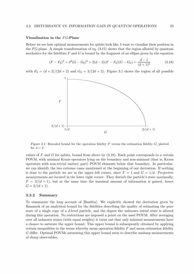
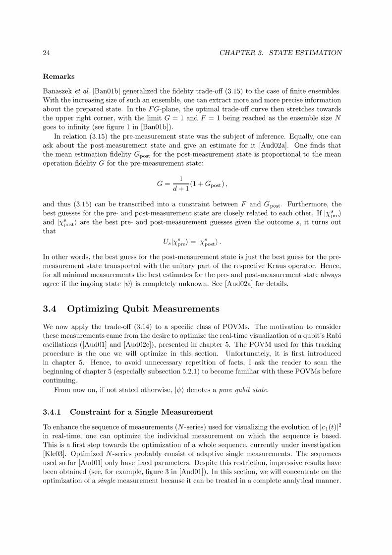
Visualization in the FG-Plane
Before we see how optimal measurements for qubits look like, I want to visualize their position inthe FG-plane. A simple transformation of eq. (3.15) shows that the region allowed by quantummechanics for the fidelities F and G is bound by the fragment of an ellipse given by the equation
(F − F0)2 + d2(G−G0)
2 + 2(d− 2)(F − F0)(G−G0) =d− 1
(d+ 1)2(3.18)
with F0 = (d + 2)/(2d + 2) and G0 = 3/(2d + 2). Figure 3.1 shows the region of all possible
2/(d+ 1)
1
1/d2/(d+ 1)
G
F
Figure 3.1: Rescaled bound for the operation fidelity F versus the estimation fidelity G, plottedfor d = 2.
values of F and G for qubits, bound from above by (3.18). Each point corresponds to a certainPOVM, with minimal Kraus operators lying on the boundary and non-minimal (that is, Krausoperators with non-trivial unitary part) POVM elements below that boundary. In particular,we can identify the two extreme cases mentioned at the beginning of our derivation. If nothingis done to the particle we are in the upper left corner, since F = 1 and G = 1/d. Projectivemeasurements are located in the lower right corner: They disturb the particle’s state maximally,F = 2/(d + 1), but at the same time the maximal amount of information is gained, henceG = 2/(d + 1).
3.3.2 Summary
To summarize the long account of [Ban01a]: We explicitly showed the derivation given byBanaszek of an analytical bound for the fidelities describing the quality of estimating the purestate of a single copy of a d-level particle, and the degree the unknown initial state is alteredduring this operation. No restrictions are imposed a priori on the used POVM. After averagingover all unknown states (with equal weights) it turns out that only minimal measurements havea chance to saturate the upper bound. This upper bound is subsequently obtained by applyingcertain inequalities to the terms whereby mean operation fidelity F and mean estimation fidelityG differ. Optimal POVMs saturating this upper bound seem to describe unsharp measurementsof sharp observables.
24 CHAPTER 3. STATE ESTIMATION
Remarks
Banaszek et al. [Ban01b] generalized the fidelity trade-off (3.15) to the case of finite ensembles.With the increasing size of such an ensemble, one can extract more and more precise informationabout the prepared state. In the FG-plane, the optimal trade-off curve then stretches towardsthe upper right corner, with the limit G = 1 and F = 1 being reached as the ensemble size Ngoes to infinity (see figure 1 in [Ban01b]).
In relation (3.15) the pre-measurement state was the subject of inference. Equally, one canask about the post-measurement state and give an estimate for it [Aud02a]. One finds thatthe mean estimation fidelity Gpost for the post-measurement state is proportional to the meanoperation fidelity G for the pre-measurement state:
G =1
d+ 1(1 +Gpost) ,
and thus (3.15) can be transcribed into a constraint between F and Gpost. Furthermore, thebest guesses for the pre- and post-measurement state are closely related to each other. If |χspre〉and |χspost〉 are the best pre- and post-measurement guesses given the outcome s, it turns outthat
Us|χspre〉 = |χspost〉 .
In other words, the best guess for the post-measurement state is just the best guess for the pre-measurement state transported with the unitary part of the respective Kraus operator. Hence,for all minimal measurements the best estimates for the pre- and post-measurement state alwaysagree if the ingoing state |ψ〉 is completely unknown. See [Aud02a] for details.
3.4 Optimizing Qubit Measurements
We now apply the trade-off (3.14) to a specific class of POVMs. The motivation to considerthese measurements came from the desire to optimize the real-time visualization of a qubit’s Rabioscillations ([Aud01] and [Aud02c]), presented in chapter 5. The POVM used for this trackingprocedure is the one we will optimize in this section. Unfortunately, it is first introducedin chapter 5. Hence, to avoid unnecessary repetition of facts, I ask the reader to scan thebeginning of chapter 5 (especially subsection 5.2.1) to become familiar with these POVMs beforecontinuing.
From now on, if not stated otherwise, |ψ〉 denotes a pure qubit state.
3.4.1 Constraint for a Single Measurement
To enhance the sequence of measurements (N -series) used for visualizing the evolution of |c1(t)|2in real-time, one can optimize the individual measurement on which the sequence is based.This is a first step towards the optimization of a whole sequence, currently under investigation[Kle03]. Optimized N -series probably consist of adaptive single measurements. The sequencesused so far [Aud01] only have fixed parameters. Despite this restriction, impressive results havebeen obtained (see, for example, figure 3 in [Aud01]). In this section, we will concentrate on theoptimization of a single measurement because it can be treated in a complete analytical manner.
3.4. OPTIMIZING QUBIT MEASUREMENTS 25
One N -series consists of N single measurements, each given by the set Ms of Krausoperators (0 ≤ p0, p1 ≤ 1)
M+ =√p0|0〉〈0| +
√p1|1〉〈1|
M− =√
1 − p0|0〉〈0| +√
1 − p1|1〉〈1| ,representing a weak measurement of some ordinary observable, e.g. energy or spin. Therefore itis of the same structure as example (3.17). Moreover, it is a non-adaptive scheme since p0 andp1 (equivalently p and ∆p; we use these two parametrizations interchangeably) are fixed for theduration of the experiment, that is, all N -series. Optimizing this POVM is a straightforwardapplication of result (3.14). We choose p1 ≥ p0 without restriction of generality.
The optimality condition (3.14) reduces for d = 2 to
f =[√
g +√
2 − g]2. (3.19)
Calculating f and g yields
f =∑
s=±|tr[Ms]|2
= (√p0 +
√p1)
2 + (√
1 − p0 +√
1 − p1)2
= 2(1 +√p0p1 +
√
(1 − p0)(1 − p1)) ,
and accordingly (remember that Es = M †sMs)
g =∑
s=±max〈ψs|Es|ψs〉
= p1 + 1 − p0 .
With this, the fidelity balance (3.19) reads√p0p1 +
√
(1 − p0)(1 − p1) =√
1 − (p0 − p1)2 .
Above equation has two solutions: p0 = p1 (⇔ ∆p = 0) corresponds to the trivial POVM withEs ∝
and is therefore excluded. Optimal single measurements for qubits are thus described by
p0 + p1 = 1 ⇔ p =1
2. (3.20)
Besides trivial measurements, projective measurements are optimal too. With p = 1/2 fixed,∆p remains the only free parameter. What does that mean? Do these two parameters have anintuitive meaning? Let us return to the FG-plane to answer these questions.
3.4.2 Partitioning the FG-Plane
We have to parametrize F and G with p and ∆p to see their working in the FG-plane. Startingfrom the results (3.6) and (3.7),
F =1
3
(
2 +
√
p2 − 1
4∆p2 +
√
(1 − p)2 − 1
4∆p2
)
(3.21)
G =1
6(3 + ∆p) . (3.22)
26 CHAPTER 3. STATE ESTIMATION
G in (3.22) measures the (average) resemblance of the guess with the unknown state, thatis, our knowledge about it. The more knowledge we obtain about a state, the more it getsdisturbed. Consequently, we can associate with ∆p the parameter displaying the strength5 of ameasurement. No measurement (and therefore no information about the state) corresponds to∆p = 0 whereas projective measurements (and maximal information) have ∆p = 1, cf. figure3.1. Unfortunately, no such concrete meaning for p has been found.
Given ∆p and p to construct any desired qubit POVM with Kraus operators M±, wheredo they lie in the FG-plane? An answer to this question will illuminate the position of minimalmeasurements in the FG-plane and the meaning of p.
To simplify our discussion, we plug (3.22) into (3.21) and obtain the following array of curves,
F (G, p) =1
3
(
2 +
√
p2 − 9(G − 1
2)2 +
√
(1 − p)2 − 9(G − 1
2)2
)
, (3.23)
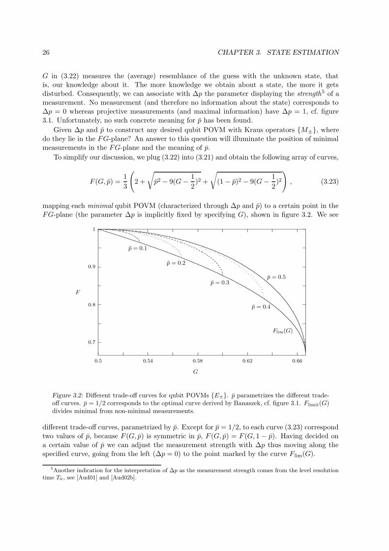
mapping each minimal qubit POVM (characterized through ∆p and p) to a certain point in theFG-plane (the parameter ∆p is implicitly fixed by specifying G), shown in figure 3.2. We see
p = 0.2
p = 0.1
Flim(G)
G
F
p = 0.5
p = 0.4
p = 0.3
0.54 0.58 0.62 0.660.5
1
0.9
0.8
0.7
Figure 3.2: Different trade-off curves for qubit POVMs E±. p parametrizes the different trade-off curves. p = 1/2 corresponds to the optimal curve derived by Banaszek, cf. figure 3.1. Flimit(G)divides minimal from non-minimal measurements.
different trade-off curves, parametrized by p. Except for p = 1/2, to each curve (3.23) correspondtwo values of p, because F (G, p) is symmetric in p, F (G, p) = F (G, 1 − p). Having decided ona certain value of p we can adjust the measurement strength with ∆p thus moving along thespecified curve, going from the left (∆p = 0) to the point marked by the curve Flim(G).
5Another indication for the interpretation of ∆p as the measurement strength comes from the level resolutiontime Tlr, see [Aud01] and [Aud02b].
3.4. OPTIMIZING QUBIT MEASUREMENTS 27
Minimal vs. Non-Minimal
At this point, (3.23) is imaginary. No combination of values 0 ≤ p ≤ 1 and 0 ≤ ∆p ≤ 1 can breakthis ‘barrier’ set by Flim(G). In other words, no minimal POVM Es can possibly lie belowthis limiting curve. Only non-minimal measurements can be found there. We thus narroweddown the region in the FG-plane where those measurements are found.
Let us specify this last statement more precisely. Setting one root term in (3.23) equal tozero and plugging the result p = 3(G − 1/2) back in yields
Flim(G) =1
3
(
2 +
√
1 − 6(G− 1
2)
)
,1
2≤ G ≤ 2
3.
With this finding, we can describe the distribution of minimal and non-minimal POVMs withinthe FG-plane, cf. figure 3.2: The absolute upper bound is set by the optimal curve F (G, p = 1/2),corresponding to all minimal POVMs fulfilling (3.20). No other minimal qubit POVM canimprove that. Also minimal, but less effective, are all POVMs represented by F (G, p), lyingbetween F (G, 1/2) and Flim(G). The latter curve identifies the lower boundary for minimalmeasurements. Below this point, only non-minimal POVMs can be found.
But it is wrong to think that only minimal POVMs lie within the slice bordered by F (G, 1/2)and Flim(G).
Unitary Back-Action
Suppose we take some minimal POVM Es. In the FG-plane one point corresponds to it,characterized by certain values of p and ∆p or, equivalently, F and G. Now, we modify theKraus operators |Ms| by unitary operations Us,
|Ms| Us−→M ′s = Us|Ms| .
Formally, this back-action Us renders the POVM non-minimal and our point within the sliceshould presumably move somewhere outside this region. But this is, in general, not true.
From (3.6) and (3.7) we know that
F =1
d(d + 1)
(
d+
N∑
s=1
|tr[Ms]|2)
, G =1
d(d+ 1)
(
d+
N∑
s=1
〈ψs|Es|ψs〉)
.
Now G only depends on the effects Es and is therefore independent of Us (cf. equations (2.10)and (2.11) on p. 10), whereas unitary parts influence the mean operation fidelity. They reducethe value of F as we saw from our derivation of the optimal trade-off, cf. estimate (3.8). Hence,our point within the slice of the FG-plane moves vertically downward by some amount δF ,depending exclusively on the unitary back-action Us. It now can happen that δF = F − F ′ issuch that the point (F ′, G), representing the POVM E ′
s, lies again within the slice with somecurve F ′(G, p′) going through it. Thus, certain non-minimal POVMs can be transformed intominimal ones by a suitable choice of p, compensating for the unitary part Us.
We saw that an appropriate choice of of p can ‘compensate’ certain types of unitary back-action, thus rendering it useless. Next, however, emphasis on these Us has to be put, becausethey can work in favor of an enhanced mean operation fidelity.

28 CHAPTER 3. STATE ESTIMATION
Chapter 4
Partial Reversal of a Non-Unitary
Operation by Unitary Back-Action
We showed in the last section that any non-minimal measurement cannot improve the trade-offbetween information gain and disturbance. The argument (3.8) is based on the assumption thatnothing is known a priori about the quantum state |ψ〉, except that it is a pure state.
What happens if something is known about the state before measuring it? In particular,we are interested in the following question: Given some a priori information about the initialpure quantum state, is it possible to improve the mean operation fidelity using non-minimalmeasurements?
This question is not only of academic interest, but has practical significance in quantumcomputational tasks. Possessing the capability to partly reduce disturbances caused by non-unitary processes (e.g. unavoidable noise, imperfect wires, etc.) with unitary quantum gatescould be a desirable feature of future quantum computers. At first sight, this seems unlikely,because of the inherent different nature of non-unitary and unitary operations. However, we willsee that there exist unitary operations canceling specific non-unitary operations to some extent,thereby increasing the fidelity.
Why are we focusing on F and not on the trade-off between F and G? Certainly, to everymean operation fidelity F corresponds a mean estimation fidelity G, but we will not bother withit for two reasons: First, G depends only on effects, is therefore independent of unitary back-action terms. Second, a priori information influences the guess for |ψ〉, hence G depends on theknowledge we have about the state. However, incorporating this knowledge into our guess is aquite complicated issue we shall not be concerned with: The best guess, that is, the eigenvectorof Es to the highest eigenvalue, is only valid when nothing is known about |ψ〉 in advance; incase of a priori information, this estimation strategy does not have to be optimal.
We will deal with qubits throughout this chapter and the qubit POVM E± introduced insubsection 3.4.1. In particular, we choose p1 ≥ p0 without restriction of generality.
4.1 A Trivial Example
Let me clarify the idea behind this cancellation procedure by a trivial example. Suppose wemeasure a known pure state |ψ〉 with a minimal Kraus operator
√Es, |ψs〉 =
√Es|ψ〉/
√ps. Since
the initial state and the operation are known, we can write down, given the orthonormal bases
29
30CHAPTER 4. NON-UNITARY OPERATION PARTLY REVERSED BY UNITARY MEANS
|ψ〉, |ψ⊥〉 and |ψs〉, |ψ⊥s 〉, the unitary operation Us = |ψ〉〈ψs|+ |ψ⊥〉〈ψ⊥
s | restoring the initialstate. By construction, Us is unitary. It maps the measured state and its orthogonal complementto their respective initial counterparts. Effectively, the action of a minimal measurement hasbeen countermanded,
|ψ〉√Es−−−→ |ψs〉 Us−→ |ψ〉 .
Of course, no information has been obtained from |ψ〉 through measurement, since everythingwas known in advance. This fact makes it possible to construct such a unitary operation. Ifwe do not know anything about |ψ〉 in the first place, this feat would – has to – be impossible.Otherwise information would be obtained without any disturbance. The state |ψ〉 could thus becloned which is prohibited by the no-cloning theorem [Woo82].
4.2 Incorporating a Priori Information
Our task consists of two parts: (1) representing knowledge about the pre-measurement statewithin the fidelity picture, and (2) constructing some unitary back-action Us given this informa-tion. In the following discussions, we will make use of the Bloch sphere. The reader not familiarwith this picture is referred to Appendix B.
4.2.1 Confining the Integration Volume
From the definition (3.4) on page 17 we already know how to include a priori information intothe mean operation fidelity,
F =
∫
dψ p(ψ)∑
s=±|〈ψ|Ms|ψ〉|2 .
It is the probability distribution p(ψ) which represents our knowledge about the pre-measurementstate. If nothing is known in advance, it is reasonable to assume equipartition, that is, eachstate has the same probability 1/4π.
Given a general probability distribution p(ψ) over the surface of the Bloch sphere and a qubitPOVM Es, we can, in principle, calculate F . However, this will only be possible analyticallyfor a few cases. We therefore restrict ourselves to a more special case of a priori information.We assume that the initial state lies – with equal probability – somewhere within a well definedregion Ω, given by
Ω := (θ, ϕ) : θ1 ≤ θ ≤ θ2 ∧ ϕ1 ≤ ϕ ≤ ϕ2 with θi ∈ [0, π], ϕi ∈ [0, 2π] .For θ1 = 0, θ2 = π and ϕ1 = 0, ϕ2 = 2π we recover the whole surface of the Bloch sphere. The‘sharp edges’ of Ω are not necessarily unphysical. Take, for example, a polarizer used in someoptical experiment. We want to make a statement about the polarization of the passed photon.But due to the polarizer’s imperfect nature any adjusted direction is only known within somemargin of error. We therefore know the polarization of the photon to be within a well definedregion Ω (in general, equipartition of polarization angles within Ω is not given, but we assumeit here for simplicity).
With this restriction, we denote the modified fidelity by
FΩ(Ms) :=1
N(Ω)
∫
Ωdψ∑
s=±|〈ψ|Ms|ψ〉|2 . (4.1)
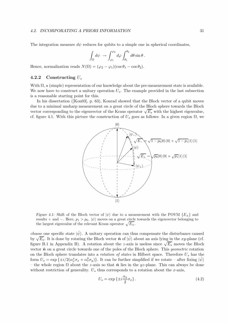
4.2. INCORPORATING A PRIORI INFORMATION 31
The integration measure dψ reduces for qubits to a simple one in spherical coordinates,
∫
Ωdψ →
∫ ϕ2
ϕ1
dϕ
∫ θ2
θ1
dθ sin θ .
Hence, normalization reads N(Ω) = (ϕ2 − ϕ1)(cos θ1 − cos θ2).
4.2.2 Constructing Us
With Ω, a (simple) representation of our knowledge about the pre-measurement state is available.We now have to construct a unitary operation Us. The example provided in the last subsectionis a reasonable starting point for this.
In his dissertation ([Kon03], p. 63), Konrad showed that the Bloch vector of a qubit movesdue to a minimal unsharp measurement on a great circle of the Bloch sphere towards the Blochvector corresponding to the eigenvector of the Kraus operator
√Es with the highest eigenvalue,
cf. figure 4.1. With this picture the construction of Us goes as follows: In a given region Ω, we
|ψ〉
|ψ−〉
|ψ+〉
|0〉
|1〉
√
E− =√
1 − p0|0〉〈0| +√
1 − p1|1〉〈1|
√
E+ =√p0|0〉〈0| + √
p1|1〉〈1|
Figure 4.1: Shift of the Bloch vector of |ψ〉 due to a measurement with the POVM E± andresults + and −. Here, p1 > p0. |ψ〉 moves on a great circle towards the eigenvector belonging tothe largest eigenvalue of the relevant Kraus operator
√
E±.
choose one specific state |ψ〉. A unitary operation can thus compensate the disturbance causedby
√Es. It is done by rotating the Bloch vector n of |ψ〉 about an axis lying in the xy-plane (cf.
figure B.1 in Appendix B). A rotation about the z-axis is useless since√Es moves the Bloch
vector n on a great circle towards one of the poles of the Bloch sphere. This geometric rotationon the Bloch sphere translates into a rotation of states in Hilbert space. Therefore Us has theform Us = exp ±i/2(αxsσx + αysσy). It can be further simplified if we rotate – after fixing |ψ〉– the whole region Ω about the z-axis so that n lies in the yz-plane. This can always be donewithout restriction of generality. Us thus corresponds to a rotation about the x-axis,
Us = exp ±iαs2σx . (4.2)
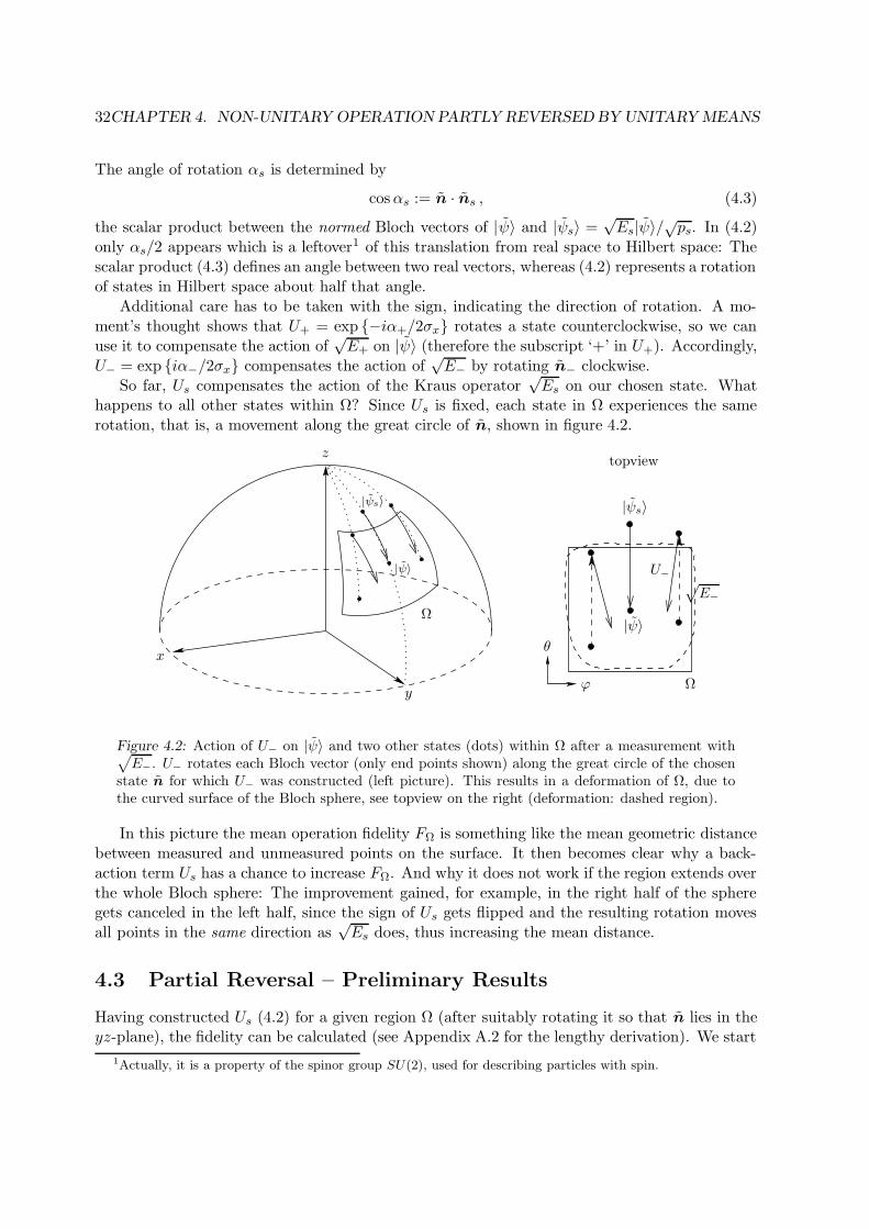
32CHAPTER 4. NON-UNITARY OPERATION PARTLY REVERSED BY UNITARY MEANS
The angle of rotation αs is determined by
cosαs := n · ns , (4.3)
the scalar product between the normed Bloch vectors of |ψ〉 and |ψs〉 =√Es|ψ〉/√ps. In (4.2)
only αs/2 appears which is a leftover1 of this translation from real space to Hilbert space: Thescalar product (4.3) defines an angle between two real vectors, whereas (4.2) represents a rotationof states in Hilbert space about half that angle.
Additional care has to be taken with the sign, indicating the direction of rotation. A mo-ment’s thought shows that U+ = exp −iα+/2σx rotates a state counterclockwise, so we canuse it to compensate the action of
√E+ on |ψ〉 (therefore the subscript ‘+’ in U+). Accordingly,
U− = exp iα−/2σx compensates the action of√E− by rotating n− clockwise.
So far, Us compensates the action of the Kraus operator√Es on our chosen state. What
happens to all other states within Ω? Since Us is fixed, each state in Ω experiences the samerotation, that is, a movement along the great circle of n, shown in figure 4.2.
y
Ω
z
x
topview
Ω
U−√
E−
|ψs〉
ϕ
θ
|ψs〉
|ψ〉
|ψ〉
Figure 4.2: Action of U− on |ψ〉 and two other states (dots) within Ω after a measurement with√
E−. U− rotates each Bloch vector (only end points shown) along the great circle of the chosenstate n for which U− was constructed (left picture). This results in a deformation of Ω, due tothe curved surface of the Bloch sphere, see topview on the right (deformation: dashed region).
In this picture the mean operation fidelity FΩ is something like the mean geometric distancebetween measured and unmeasured points on the surface. It then becomes clear why a back-action term Us has a chance to increase FΩ. And why it does not work if the region extends overthe whole Bloch sphere: The improvement gained, for example, in the right half of the spheregets canceled in the left half, since the sign of Us gets flipped and the resulting rotation movesall points in the same direction as
√Es does, thus increasing the mean distance.
4.3 Partial Reversal – Preliminary Results
Having constructed Us (4.2) for a given region Ω (after suitably rotating it so that n lies in theyz-plane), the fidelity can be calculated (see Appendix A.2 for the lengthy derivation). We start
1Actually, it is a property of the spinor group SU(2), used for describing particles with spin.
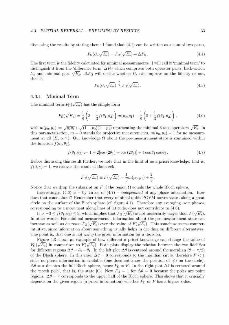
4.3. PARTIAL REVERSAL – PRELIMINARY RESULTS 33
discussing the results by stating them: I found that (4.1) can be written as a sum of two parts,
FΩ(Us√
Es) = FΩ(√
Es) + ∆FΩ . (4.4)
The first term is the fidelity calculated for minimal measurements. I will call it ‘minimal term’ todistinguish it from the ‘difference term’ ∆FΩ which comprises both operator parts, back-actionUs and minimal part
√Es. ∆FΩ will decide whether Us can improve on the fidelity or not,
that is
FΩ(Us√
Es)?≥ FΩ(
√
Es) . (4.5)
4.3.1 Minimal Term
The minimal term FΩ(√Es) has the simple form
FΩ(√
Es) =1
8
(
3 − 1
3f(θ1, θ2)
)
m(p0, p1) +1
8
(
5 +1
3f(θ1, θ2)
)
, (4.6)
with m(p0, p1) :=√p0p1 +
√
(1 − p0)(1 − p1) representing the minimal Kraus operators√Es. In
this parametrization, m = 0 stands for projective measurements, m(p0, p0) = 1 for no measure-ment at all (Es ∝
). Our knowledge Ω about the pre-measurement state is contained withinthe function f(θ1, θ2),
f(θ1, θ2) := 1 + 2[cos (2θ1) + cos (2θ2)] + 4 cos θ1 cos θ2 . (4.7)
Before discussing this result further, we note that in the limit of no a priori knowledge, that is,f(0, π) = 1, we recover the result of Banaszek,
FΩ(√
Es) ≡ F (√
Es) =1
3m(p0, p1) +
2
3.
Notice that we drop the subscript on F if the region Ω equals the whole Bloch sphere.Interestingly, (4.6) is – by virtue of (4.7) – independent of any phase information. How
does that come about? Remember that every minimal qubit POVM moves states along a greatcircle on the surface of the Bloch sphere (cf. figure 4.1). Therefore any averaging over phases,corresponding to a movement along lines of latitude, does not contribute to (4.6).
It is −3 ≤ f(θ1, θ2) ≤ 9, which implies that FΩ(√Es) is not necessarily larger than F (
√Es).
In other words: For minimal measurements, information about the pre-measurement state canincrease as well as decrease FΩ(
√Es) over the value of F (
√Es). This somehow seems counter-
intuitive, since information about something usually helps in deciding on different alternatives.The point is, that one is not using the given information for a decision.
Figure 4.3 shows an example of how different a priori knowledge can change the value ofFΩ(
√Es) in comparison to F (
√Es). Both plots display the relation between the two fidelities
for different regions ∆θ = θ2 − θ1. In the left plot ∆θ is centered around the meridian (θ = π/2)of the Bloch sphere. In this case, ∆θ = 0 corresponds to the meridian circle; therefore F < 1since no phase information is available (one does not know the position of |ψ〉 on the circle).∆θ = π denotes the full Bloch sphere, hence FΩ = F . In the right plot ∆θ is centered aroundthe ‘north pole’, that is, the state |0〉. Now FΩ = 1 for ∆θ = 0 because the poles are pointregions. ∆θ = π corresponds to the upper half of the Bloch sphere. This shows that it cruciallydepends on the given region (a priori information) whether FΩ or F has a higher value.
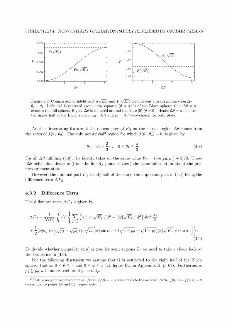
34CHAPTER 4. NON-UNITARY OPERATION PARTLY REVERSED BY UNITARY MEANS
F (√Es)
FΩ(√Es)
FΩ(√Es)
F (√Es)
0.958
0.962
0.966
0.97
0 1 2 3
0.974
∆θ
F
1
0 1 2 3
∆θ
F
0.96
0.97
0.98
0.99
Figure 4.3: Comparison of fidelities FΩ(√Es) and F (
√Es) for different a priori information ∆θ =
θ2 − θ1. Left: ∆θ is centered around the equator (θ = π/2) of the Bloch sphere; thus ∆θ = πdenotes the full sphere. Right: ∆θ is centered around the state |0〉 (θ = 0). Hence ∆θ = π denotesthe upper half of the Bloch sphere. p0 = 0.3 and p1 = 0.7 were chosen for both plots.
Another interesting feature of the dependency of FΩ on the chosen region ∆θ comes fromthe zeros of f(θ1, θ2). The only non-trivial2 region for which f(θ1, θ2) = 0, is given by
θ2 = θ1 +2
3π , 0 ≤ θ1 ≤ π
3. (4.8)
For all ∆θ fulfilling (4.8), the fidelity takes on the same value FΩ = (3m(p0, p1) + 5)/8. These‘∆θ-belts’ thus describe (from the fidelity point of view) the same information about the pre-measurement state.
However, the minimal part FΩ is only half of the story, the important part in (4.4) being thedifference term ∆FΩ.
4.3.2 Difference Term
The difference term ∆FΩ is given by
∆FΩ =1
N(Ω)
∫
Ωdψ
∑
s=±
(
|〈ψ|σx√
Es|ψ〉|2 − |〈ψ|√
Es|ψ〉|2)
sin2 αs2
+1
2〈ψ|σy|ψ〉
[
(√p1 −
√p0)〈ψ|
√
E+|ψ〉 sinα+ + (√
1 − p0 −√
1 − p1)〈ψ|√
E−|ψ〉 sinα−]
.
(4.9)
To decide whether inequality (4.5) is true for some regions Ω, we need to take a closer look atthe two terms in (4.9).
For the following discussion we assume that Ω is restricted to the right half of the Blochsphere, that is, 0 ≤ θ ≤ π and 0 ≤ ϕ ≤ π (cf. figure B.1 in Appendix B, p. 67). Furthermore,p1 ≥ p0 without restriction of generality.
2That is, no point regions or circles. f(π/2, π/2) = −3 corresponds to the meridian circle, f(0, 0) = f(π, π) = 9correspond to points |0〉 and |1〉, respectively.
4.3. PARTIAL REVERSAL – PRELIMINARY RESULTS 35
Term 2
The second term in (4.9) reads
1
2〈ψ|σy |ψ〉
[
(√p1 −
√p0)〈ψ|
√
E+|ψ〉 sinα+ + (√
1 − p0 −√
1 − p1)〈ψ|√
E−|ψ〉 sinα−]
. (4.10)
〈ψ|σy |ψ〉 =: y equals the y-component of the Bloch vector of |ψ〉. It is y ≥ 0 because of ourchoice of Ω (if |ψ〉 lies in the xz-plane, y = 0). Going on to the bracket-term [·] we note that√p1 −√
p0 ≥ 0 and√
1 − p0 −√
1 − p1 ≥ 0.√Es are positive operators, so by definition (this
is independent of our choice of Ω) 〈ψ|√Es|ψ〉 ≥ 0. The two rotation angles αs are confined tothe interval 0 ≤ αs < π, and thus sinαs ≥ 0 (αs = 0 would mean that |ψ〉 lies in one of thepoles of the Bloch sphere. αs ≈ π calls for a projective measurement, transporting, for example,|ψ〉 ≈ |1〉 to the antipodal state |0〉).
Given our assumptions, (4.10) is greater or equal to zero. The bracket term [·] is herebygreater or equal to zero, independent of Ω.
Term 1
For both3 parts of the sum
∑
s=±
(
|〈ψ|σx√
Es|ψ〉|2 − |〈ψ|√
Es|ψ〉|2)
sin2 αs2
(4.11)
to be positive, we need to decide whether |〈ψ|σx√Es|ψ〉|2−|〈ψ|√Es|ψ〉|2 ≥ 0 or not. To this end
we rewrite the terms in the difference as scalar products which can be interpreted geometrically.Out of that interpretation will then arise physical conditions. The following argumentation isvalid for either s = + or s = −.
We start by defining the pure states
|ψ′〉 :=√
Es|ψ〉/√ps and |ψ′′〉 := σx|ψ′〉 ,
having (since σx is unitary) norm equal to one, 〈ψ′|ψ′〉 = 〈ψ′′|ψ′′〉 = 1. Thus,
|〈ψ|σx√
Es|ψ〉|2 − |〈ψ|√
Es|ψ〉|2 = ps
(
|〈ψ|ψ′′〉|2 − |〈ψ|ψ′〉|2)
. (4.12)
Subsequently, we omit the factor ps > 0 since it is irrelevant for deciding if (4.11) can be greaterthan zero for certain POVMs and regions Ω. For a geometrical representation we rewrite (4.12)using Bloch vectors: With (cf. Appendix B, p. 67)
ρ′ =1
2(
+ n′ · σ) , ρ′′ =
1
2(
+ n′′ · σ)
and the identity tr[ρρ′] = |〈ψ|ψ′〉|2, (4.12) reads
|〈ψ|ψ′′〉|2 − |〈ψ|ψ′〉|2 = tr[ρρ′′] − tr[ρρ′]
=1
2(n · n′′ − n · n′) . (4.13)
3To decide whether one part of the sum is larger than the other is a far more difficult question to answer.
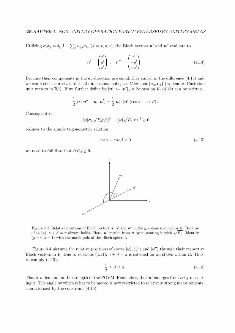
36CHAPTER 4. NON-UNITARY OPERATION PARTLY REVERSED BY UNITARY MEANS
Utilizing σiσj = δij
+∑
k εijkσk, (k = x, y, z), the Bloch vectors n′ and n′′ evaluate to
n′ =
x′
y′
z′
, n′′ =
x′
−y′−z′
. (4.14)
Because their components in the ex-direction are equal, they cancel in the difference (4.13) andwe can restrict ourselves to the 2-dimensional subspace V := spaney, ez (ei denotes Cartesianunit vectors in 3). If we further define by |n′| := |n′|V a 2-norm on V, (4.13) can be written
1
2(n · n′′ − n · n′) =
1
2|n| · |n′|(cos γ − cos β) .
Consequently,
|〈ψ|σx√
Es|ψ〉|2 − |〈ψ|√
Es|ψ〉|2 ≥ 0
reduces to the simple trigonometric relation
cos γ − cos β ≥ 0 (4.15)
we need to fulfill so that ∆FΩ ≥ 0.
y
z
n
n′
βγ
n′′
Figure 4.4: Relative positions of Bloch vectors n, n′ and n′′ in the yz-plane spanned by V . Becauseof (4.14), γ + β = π always holds. Here, n′ results from n by measuring it with
√
E+ (identify(y = 0, z = 1) with the north pole of the Bloch sphere).
Figure 4.4 pictures the relative positions of states |ψ〉, |ψ ′〉 and |ψ′′〉 through their respectiveBloch vectors in V. Due to relations (4.14), γ + β = π is satisfied for all states within Ω. Thus,to comply (4.15),
π
2≤ β < π . (4.16)
That is a demand on the strength of the POVM. Remember, that n′ emerges from n by measur-ing it. The angle by which n has to be moved is now restricted to relatively strong measurements,characterized by the constraint (4.16).
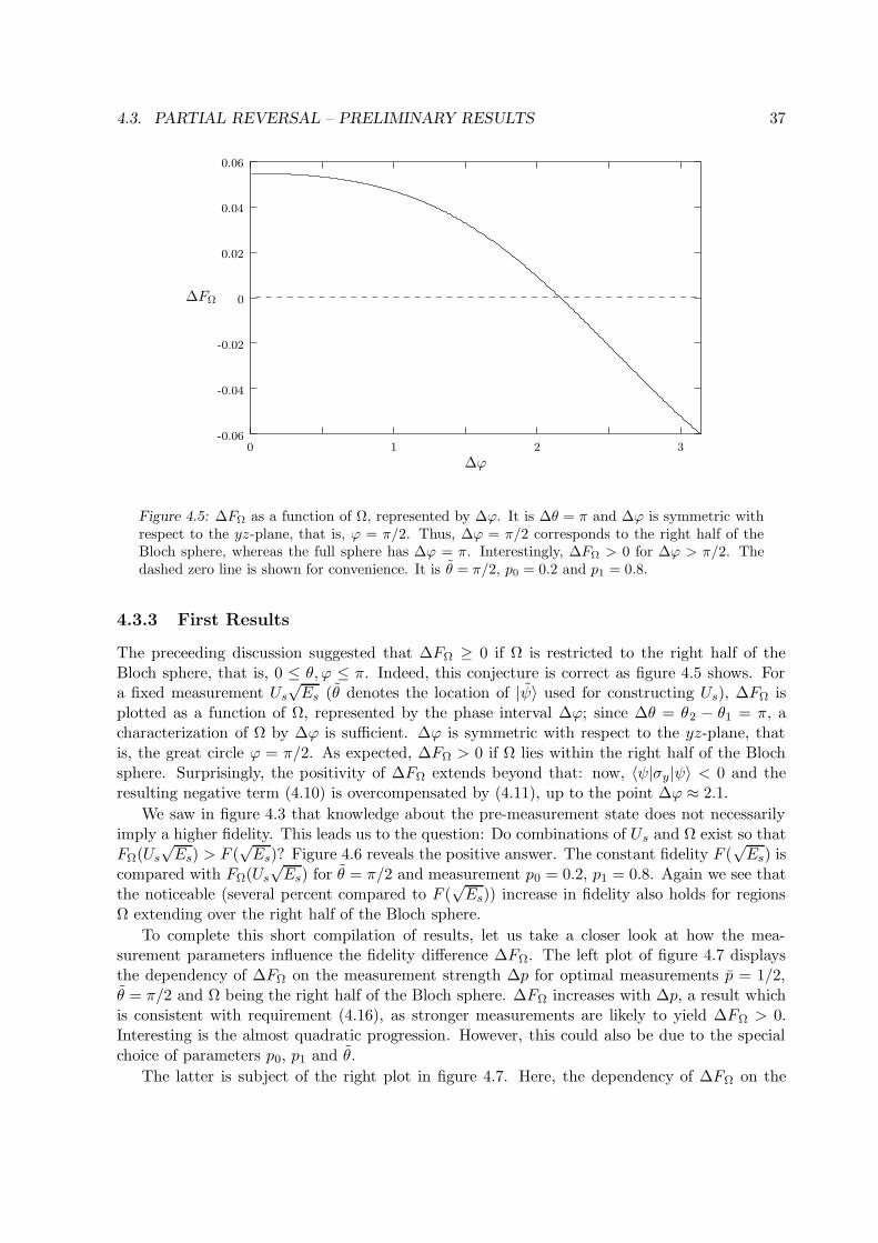
4.3. PARTIAL REVERSAL – PRELIMINARY RESULTS 37
-0.06
-0.04
-0.02
0
0.02
0.04
0.06
0 1 2 3
∆ϕ
∆FΩ
Figure 4.5: ∆FΩ as a function of Ω, represented by ∆ϕ. It is ∆θ = π and ∆ϕ is symmetric withrespect to the yz-plane, that is, ϕ = π/2. Thus, ∆ϕ = π/2 corresponds to the right half of theBloch sphere, whereas the full sphere has ∆ϕ = π. Interestingly, ∆FΩ > 0 for ∆ϕ > π/2. Thedashed zero line is shown for convenience. It is θ = π/2, p0 = 0.2 and p1 = 0.8.
4.3.3 First Results
The preceeding discussion suggested that ∆FΩ ≥ 0 if Ω is restricted to the right half of theBloch sphere, that is, 0 ≤ θ, ϕ ≤ π. Indeed, this conjecture is correct as figure 4.5 shows. Fora fixed measurement Us
√Es (θ denotes the location of |ψ〉 used for constructing Us), ∆FΩ is
plotted as a function of Ω, represented by the phase interval ∆ϕ; since ∆θ = θ2 − θ1 = π, acharacterization of Ω by ∆ϕ is sufficient. ∆ϕ is symmetric with respect to the yz-plane, thatis, the great circle ϕ = π/2. As expected, ∆FΩ > 0 if Ω lies within the right half of the Blochsphere. Surprisingly, the positivity of ∆FΩ extends beyond that: now, 〈ψ|σy|ψ〉 < 0 and theresulting negative term (4.10) is overcompensated by (4.11), up to the point ∆ϕ ≈ 2.1.
We saw in figure 4.3 that knowledge about the pre-measurement state does not necessarilyimply a higher fidelity. This leads us to the question: Do combinations of Us and Ω exist so thatFΩ(Us
√Es) > F (
√Es)? Figure 4.6 reveals the positive answer. The constant fidelity F (
√Es) is
compared with FΩ(Us√Es) for θ = π/2 and measurement p0 = 0.2, p1 = 0.8. Again we see that
the noticeable (several percent compared to F (√Es)) increase in fidelity also holds for regions
Ω extending over the right half of the Bloch sphere.
To complete this short compilation of results, let us take a closer look at how the mea-surement parameters influence the fidelity difference ∆FΩ. The left plot of figure 4.7 displaysthe dependency of ∆FΩ on the measurement strength ∆p for optimal measurements p = 1/2,θ = π/2 and Ω being the right half of the Bloch sphere. ∆FΩ increases with ∆p, a result whichis consistent with requirement (4.16), as stronger measurements are likely to yield ∆FΩ > 0.Interesting is the almost quadratic progression. However, this could also be due to the specialchoice of parameters p0, p1 and θ.
The latter is subject of the right plot in figure 4.7. Here, the dependency of ∆FΩ on the
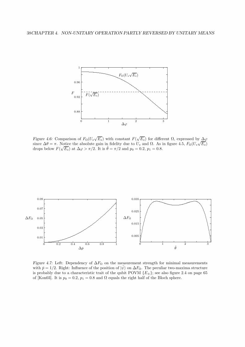
38CHAPTER 4. NON-UNITARY OPERATION PARTLY REVERSED BY UNITARY MEANS
F (√Es)
FΩ(Us
√Es)
0.88
0.92
0.96
1
0 1 2 3
F
∆ϕ
Figure 4.6: Comparison of FΩ(Us
√Es) with constant F (
√Es) for different Ω, expressed by ∆ϕ
since ∆θ = π. Notice the absolute gain in fidelity due to Us and Ω. As in figure 4.5, FΩ(Us
√Es)
drops below F (√Es) at ∆ϕ > π/2. It is θ = π/2 and p0 = 0.2, p1 = 0.8.
0.005
0.015
0.025
0.035
0 1 2 3
θ
0.01
0.03
0.05
0.07
0.09
0 0.2 0.4 0.6 10.8
∆p
∆FΩ∆FΩ
Figure 4.7: Left: Dependency of ∆FΩ on the measurement strength for minimal measurementswith p = 1/2. Right: Influence of the position of |ψ〉 on ∆FΩ. The peculiar two-maxima structureis probably due to a characteristic trait of the qubit POVM E±; see also figure 2.4 on page 65of [Kon03]. It is p0 = 0.2, p1 = 0.8 and Ω equals the right half of the Bloch sphere.
4.3. PARTIAL REVERSAL – PRELIMINARY RESULTS 39
position θ of our chosen state |ψ〉 is investigated. The prominent feature is the two-maximastructure. This could be due to the special POVM we used in our calculations, see also figure2.4 on page 65 of [Kon03]. The structure gets unsymmetrical if the measurements become non-optimal, that is, p 6= 1/2. However, numerical examples indicate that a change of ∆p and Ω donot destroy this feature.
The results found here allow for a more thorough investigation. Ideas for further work aregiven in the outlook, see chapter 7.

40CHAPTER 4. NON-UNITARY OPERATION PARTLY REVERSED BY UNITARY MEANS
Chapter 5
Intermezzo: Real-Time Visualization
of Rabi-Oscillations using Weak
Measurements
As the title already indicates this chapter is intended as a transition from questions relatedto state estimation towards parameter estimation discussed in chapter 6. So far we discussedquantum state estimation and the optimal trade-off between information gain and disturbance.From this compromise we derived optimal measurements for qubits and investigated the influencea unitary back-action – in combination with information about the pre-measurement state – hason the fidelity.
The motivation to optimize qubit POVMs E± in section 3.4 stems from the desire to im-prove the real-time visualization of a qubit’s Rabi oscillations ([Aud01], [Aud02b] and [Aud02c]).Besides measurements, the algorithm of how to find a ‘best guess’ for the variable used to char-acterize the evolution of the monitored state can be subject to optimization. This will be thecontent of chapter 6, where we discuss – in addition to the one described in section 5.3 – twodifferent estimation schemes for the characteristic parameter |c1(t)|2.
We will first outline the overall scheme (section 5.1) before reviewing [Aud01] and, in detail,the key ingredients for our discussion of parameter estimation in the next chapter: namely thePOVM used for tracking (section 5.2) and the algorithm for estimating |c1(t)|2 (section 5.3).Section 5.4 introduces the mean square deviation D as the criterion defining the quality of aguess.
Throughout this and the following chapter we apply terminology from probability theoryused in statistical inference of parameters. See also Appendix C for a compilation of definitionsas well as [Lar83] and [Kre70] for thorough accounts.
5.1 Real-Time Monitoring in a Nutshell
Under the influence of a periodic driving potential, the resulting motion of a normalized qubitstate (Schrodinger picture)
|ψ〉 = c0(t)|0〉 + c1(t)|1〉 (5.1)
involves oscillations of the probabilities |c0(t)|2 and |c1(t)|2, called Rabi oscillations. Usuallythey are measured using projective measurements. For this purpose an ensemble is prepared
41
42 CHAPTER 5. INTERMEZZO: REAL-TIME MONITORING OF RABI OSCILLATIONS
in the initial state and a projection measurement is carried out at time t0 on each ensemblemember thus leading to the determination of |c1(t0)|2. Repeating the procedure for differenttimes result in the Rabi oscillations of |c1(t)|2.
In [Aud01] and [Aud02c] Audretsch et al. considered the situation where only one qubit isavailable and the objective is to visualize its Rabi dynamics in real-time. For this purpose thespecial class of unsharp measurements is employed.
To monitor the evolution of |c1(t)|2, the qubit is subjected to a sequence of unsharp mea-surements with a POVM E± (how unsharp a measurement has to be shall not be of concernto us here). Successive measurements are separated by a time τ > 0 during which the systemevolves freely. The duration of a measurement δτ is assumed to be much smaller than τ , thusδτ = 0 is justified. The obtained sequence (e.g. − + + − + + − − − + − − − + + − · · · ) ofmeasurement readouts is then split into M blocks of N , called N -series. From each N -series therelative frequency r = N+/N of positive results + is used to calculate a ‘best guess’ gr(tm) for|c1(tm)|2 at time tm (m = 1, . . . ,M), denoting the end of the respective N -series (for examplet1 = Nτ identifies the end of the first N -series). The sequence gr(t1), . . . , gr(tM ) represents theapproximate visualization of the qubit’s Rabi oscillations |c1(t)|2.
5.2 Single Measurement and N-Series
In classical physics it is possible to track the evolution of an individual system without disturbingit. In quantum mechanics, this can only be achieved approximately. Projective measurementsare not suited for this purpose since they severely alter the system’s dynamics. In fact, asequence of projection measurements results in the well-known Zeno effect, a suppression of theoriginal dynamics by measurement (the modified Zeno dynamics is almost perfectly traceable).In our case, Quantum Non-Demolition1 (QND) measurements are no alternative either sincethey require for non-trivial dynamics (i.e. a Hamiltonian H 6=
) an observable with continuousspectrum [Per89]. We are thus forced to resort to generalized measurements.
5.2.1 Motivating the Single Measurement E±These POVMs have to fulfill two complementary conditions:
1. The measurement must not disturb the system too much, so that its evolution remainsclose to the undisturbed case.
2. The coupling of the measurement apparatus to the qubit should nevertheless be so strongthat the readout shows accurately enough the modified dynamics of the system (includingthe disturbance by the measurement).
What kind of POVM complies with these two demands? The qubit (5.1) is given in the or-thonormed basis states |0〉, |1〉 which are eigenstates of a sharp observable A; this could be,for example, energy or spin. It is therefore advisable to consider minimal measurements whichare diagonal in that basis: We specify the measurement to have only two outcomes or pointer
1The characteristic trait of QND measurements is represented by the fact, that the system under study is atall times in an eigenstate of the measured observable. Hence the term ‘non-demolition’.
5.2. SINGLE MEASUREMENT AND N -SERIES 43
readings, denoted by + and −, with Kraus operators
M+ := u+0 |0〉〈0| + u+
1 |1〉〈1|M− := u−0 |0〉〈0| + u−1 |1〉〈1| .
We further require that u+0,1 and u−0,1 be positive. An overall phase factor exp iϕ± is omitted
without loss of generality.Why do we choose a minimal POVM which commutes with the sharp observable A of the
system?Since the measurement scheme contains consecutive measurements, the post-measurement
state should not be altered qualitatively, i.e., a superposition of states |0〉 and |1〉 should, thoughmodified, remain a superposition. We therefore require diagonality of the Kraus operators inthe |0〉, |1〉-basis.
The minimality (and therefore the positivity of u+0,1 and u−0,1) of M± ensures that there is no
unnecessary disturbance of the state (5.1). What does ‘unnecessary’ mean? Suppose we takea non-minimal Kraus operator M±. It can be split due to the polar-decomposition theoreminto a minimal part |M±| and a unitary back-action term U±. The minimal part is, becauseof its relation to the effects E± = |M±|2, connected to the acquisition of information. Theunitary evolution U± represents an additional Hamiltonian evolution not leading to any increaseof information about the system (see, for example, [Wis95]). It should therefore be set as U± =
(neglecting a global phase factor).Why U± 6=
is indeed obstructive can best be seen in the Bloch sphere picture: For thenon-minimal Kraus operators M± to be diagonalizable (to comply condition 1. on page 42),
they have to be normal, that is, [M †±,M±] = 0, which amounts to [|M±|2, U±] = 0. Hence, U±
and |M±| have to be diagonal in the same basis. Now if U± is diagonal with respect to |0〉, |1〉it can be written as U± = exp −iθ±σz for some angles θ± and σz as the Pauli operator.The resonant Rabi oscillations that our qubit (5.1) performs are represented by a rotation ofthe normalized Bloch vector in the yz-plane (given that the initial state lies in this plane). Aminimal measurement induces a change of the state within the yz-plane, cf. figure 4.1 on page31. U± on the other hand rotates the Bloch vector of |ψ〉 about the z-axis thereby leaving theyz-plane. As a consequence, U± cannot compensate the inevitable influence of |M±|. Moreover,in a sequence of measurements, U± heavily disturbs the original Rabi oscillation one is trying tovisualize. Therefore we have to choose U± =
in order to disturb the Rabi oscillations by the
action of M± as little as possible. In real experiments, any non-trivial U± can be compensatedby means of feedback (cf. Wiseman [Wis95]).
Having motivated the POVM E±, we introduce
p0 := (u+0 )2 = 1 − (u−0 )2 , p1 := (u+
1 )2 = 1 − (u−1 )2 ,
and the parameters
p :=1
2(p0 + p1) , ∆p := p1 − p0
used to characterize the single measurement. Because E± constitutes a POVM, we have0 ≤ p0, p1 ≤ 1. Assuming further p1 ≥ p0, p and ∆p are likewise confined to the unit interval.With this parametrization at hand, the POVM writes
E+ := p0|0〉〈0| + p1|1〉〈1|E− := (1 − p0)|0〉〈0| + (1 − p1)|1〉〈1| . (5.2)
44 CHAPTER 5. INTERMEZZO: REAL-TIME MONITORING OF RABI OSCILLATIONS
Accordingly, the probabilities read p± = 〈ψ|E±|ψ〉, with p+ + p− = 1. In the limiting casep0 = 0 and p1 = 1 a projection valued measure of the sharp observable A is obtained. Thus∆p = 1 corresponds to a projective measurement of A. In the opposite limit ∆p 1 theeffects are nearly proportional to the identity operator and the probabilities p± of the outcomesbecome nearly independent of the initial state. This property justifies to call the POVM E±a smeared/unsharp version of the sharp hermitian observable A.
5.2.2 One N-Series
With the POVM (5.2) at hand, we now perform on the initial state |ψ0〉 a sequence of N unsharpmeasurements with the same parameters in an immediate succession. This is called an ‘N -series’.Using the same set of parameters (p0, p1) for the whole series necessarily renders the schemenon-adaptive. The phrase ‘immediate succession’ makes the whole sequence unphysical, sinceany real measurements are separated in time by τ > 0. However, it turns out (cf. Appendix Bof [Aud01]) that the results derived from this assumption τ = 0 can be applied to the case of N -series with dynamical evolution between two single measurements if the number of measurementsN in one N -series fulfills2
(N − 1)2 maxu+0 , u
−1
2max|u+1 − u+
0 |, |u−1 − u−0 |TRπτ
. (5.3)
Here it was assumed that the matrix elements of the operation M+ satisfy u+0 > u+
1 . Otherwisethe indices 0 and 1 have to be permutated. TR denotes the Rabi period.
In the following we assume that N is chosen according to (5.3), that is, we do not have toworry about any Hamiltonian evolution of the system between two measurements. Since theKraus operators M+ and M− commute, the final state after the N -series does not depend onthe order of + and − results. For any particular sequence of results with a total number N+ ofresults + the normalized state |ψ〉 is transformed according to |ψ〉 →M(N+, N)|ψ〉 with
M(N+, N) = MN+
+ MN−N+
− .
In view of the ‘best guess’ defined in the next section, we restrict ourselves to the informationthat the total number of + results is N+, regardless of when they occurred in the sequence.That is, we are only interested in the relative frequency r := N+/N of positive results. rwill be the measurement outcome attributed to one N -series. Thus, by interpreting the N -series conceptually as one single measurement, we have to work out the effects related to thismeasurement.
The conditional probability p(N+
∣
∣N, |c1|2) that N+ positive results (given N and |c1|2) are
measured in one N -series is( NN+
)
times the probability that a particular ordered sequence of N+
positive and N −N+ negative results is obtained:
p(N+
∣
∣N, |c1|2) = 〈ψ|E(N+, N)|ψ〉 ,
2With dynamical evolution U = exp −iHτ (~ = 1) in between two measurements, the M± no longercommutate with U . This residual commutator accumulates the longer one N -series gets. Hence restriction (5.3).
5.3. BEST GUESS FOR |C1|2 45
where the effect E(N+, N) is given by
E(N+, N) =
(
N
N+
)
M †(N+, N)M(N+, N)
=
(
N
N+
)
[
pN+
0 (1 − p0)N−N+ |0〉〈0| + p
N+
1 (1 − p1)N−N+ |1〉〈1|
]
. (5.4)
The corresponding conditional probability is a linear combination of binomial distributions,
p(N+
∣
∣N, |c1|2) =
(
N
N+
)
[α0 + (α1 − α0)|c1|2] . (5.5)
Here we introduced the abbreviation αi := pN+
i (1−pi)N−N+ (i = 0, 1) and used |c0|2 = 1−|c1|2.Notice, that we only care about measurement statistics (5.5) and do not pay attention to thestate after one N -series.
5.3 Best Guess for |c1|2
So far we motivated a special POVM E±, representing a smeared version of the sharp ob-servable A, suited for the purpose of tracking the evolution of |c1(t)|2 in real-time. To this end,sequences of unsharp measurements were defined and effects for one such N -series derived. In do-ing so we conceived the series conceptually as one single measurement with POVM E(N+, N)and relative frequency r = N+/N as measurement outcome.
Now, to approximately monitor the evolution of |c1(t)|2, several N -series at different times tm(m = 1, . . . ,M) are necessary, each of them yielding a best guess we are now going to motivate.
Imagine we have an ensemble of initial states |ψ0〉 and we make measurements on this en-semble with the POVM (5.4). Then, the statistical expectation value of the relative frequencyof positive results r = N+/N is given by
〈r〉 :=
N∑
N+=0
N+
Np(N+
∣
∣N, |c1|2)
= p0|c0|2 + p1|c1|2 . (5.6)
Based on (5.6) it is easy to relate |c1|2 of the initial state with the expectation value 〈r〉 of anN -series of unsharp measurements starting with |ψ0〉,
|c1|2 =〈r〉 − p0
∆p. (5.7)
The important point here is that |c1|2 and 〈r〉 refer to an ensemble represented by the state |ψ0〉.If only one realization of |ψ0〉 is available, only one N -series can be measured and only a
best guess gr for the quantity |c1|2 can be obtained. Equation (5.7) suggests to choose3 it as
gr :=r − p0
∆p. (5.8)
3In [Aud01], gr is denoted by G1. Here, the capital letter G could be mistaken for the mean estimation fidelity.In this thesis, every guess will be denoted by g, with a subscript referring to the method of derivation.
46 CHAPTER 5. INTERMEZZO: REAL-TIME MONITORING OF RABI OSCILLATIONS
By virtue of (5.7), gr is an unbiased estimator for the unknown value of |c1|2. This propertyrepresented the main motivation for the definition of gr by equation (5.8). For r < p0, theguess (5.8) becomes negative. This seems unphysical at first, but it is the unbiasedness whichguarantees that gr fluctuates (in the long run) around the true value of |c1|2.
Although (5.8) was constructed in order to meet the unbiasedness criterion, I found analternative motivation of gr based on ensembles (the following subsection does not contain analternative derivation of gr, because gr was not derived in the first place but taken from ananalogy).
5.3.1 Motivating gr From Ensembles Using Maximum Likelihood
Suppose we are given an ensemble of N identical qubits |ψ〉 = c0|0〉+ c1|1〉. On each member ofthe ensemble a measurement is made with the same POVM E± (5.2). The aim is to calculatean estimate for |c1|2 given the sequence of N measurement results (e.g. + + −− + + − + −−−− + − · · · ). To this end, the maximum likelihood method is employed.
The maximum likelihood method for generating estimators of unknown parameters is avery powerful technique, giving – in general – ‘good’ estimators. It can be described as follows:Suppose we draw a sample x1, . . . , xN from the random variable X, whose probability functionpX(u) depends on an unknown parameter u. The maximum likelihood estimator u is thendefined as the value which maximizes the so-called likelihood function l(u) = pX(x1) · · · pX(xN ),the joint probability function of the sample, evaluated at the observed sample values x1, . . . , xN .
With the POVM E±, the probabilities to get + or − in a measurement are p+ = 〈E+〉 =p0|c0|2 + p1|c1|2 = p0 + ∆p|c1|2 and p− = 1 − p+. The estimator |c1|2 maximizes the likelihoodfunction
l(|c1|2) =
(
N
N+
)
pN+
+ (1 − p+)N−N+
=
(
N
N+
)
(p0 + ∆p|c1|2)N+(1 − p0 − ∆p|c1|2)N−N+ . (5.9)
Since we are not interested in the order of results + and −, the binomial factor( NN+
)
has to be
included. Maximizing (5.9) requires the first derivative4 to vanish,
∂l
∂|c1|2= ∆p(p0 + ∆p|c1|2)N+−1(1 − p0 − ∆p|c1|2)N−N+−1
·[
N+(1 − p0 − ∆p|c1|2) − (N −N+)(p0 + ∆p|c1|2)] !
= 0 . (5.10)
This equation has only one physically reasonable solution: ∆p = 0 can be discarded at once, justas |c1|2 = −p0/∆p and |c1|2 = (1 − p0)/∆p, derived from setting the second and third productterm in (5.10) equal to zero. Both estimators solely depend on the parameters characterizing thePOVM. Hence they are constant. In addition, −p0/∆p < 0 renders this estimator unphysical.We are thus left with the fourth term in (5.10), which gives
|c1|2ML=N+ −Np0
N∆p=r − p0
∆p= gr . (5.11)
4In general, l(|c1|2, p0,∆p,N+, N) is a function of several variables. In this special case, everything but |c1|2is fixed and we could have replaced the partial derivative by d/d|c1|2.
5.4. MEAN SQUARE DEVIATION AS MEASURE OF QUALITY 47
This peculiar result merits further discussion. Originally, gr was constructed as an unbiasedestimator, starting from the results of one N -series. That is, a sequence of measurements isconducted on one and only one state. The derivation of (5.11) started from an ensemble, thatis, N separate measurements are carried out on an ensemble of identical states. Why do bothmethods yield the same estimator?
Obviously, these two conceptually different procedures agree on the level of estimators. How-ever, in the ensemble approach, independency of measurements is guaranteed in contrast to theN -series. So both methods are not only conceptually but physically different. This fact isexpressed in the mean square deviation D (see section 5.4 for the definition):
limN→∞
D(gr) = Dprojective (5.12)
limN→∞
D(|c1|2ML) = 0 . (5.13)
In case of an infinite ensemble, an infinite amount of information is available and D(|c1|2ML) hasto go to zero (|c1|2 is known exactly). For the N -series, infinite N means infinitely many unsharpmeasurements. That is equivalent ([Kon03], p. 58) to one projective measurement. Hence, thelower limit Dprojective, derived in the forthcoming section.
To sum up: Although two physically different measurement schemes yield the same guessfor |c1|2, their dissimilarity shows up on the level of mean square deviations.
5.4 Mean Square Deviation as Measure of Quality
Experimental physicists often use the standard deviation in their statistical analysis of measureddata. This stochastic concept quantifies the variation of a measured quantity X by the averagequadratic distance of all obtained values from the measured average 〈X〉,
σ2(X) = 〈(X − 〈X〉)2〉 .
The average 〈·〉 is hereby taken with respect to the probability distribution pX underlying X.In the real-time visualization of Rabi oscillations, we are interested in an estimate g preferably
close to the actual value of |c1|2 for which a measured average no longer exists. However, wecan define – in analogy to σ2 – the mean square deviation D,
D(g) := 〈(g − |c1|2)2〉
=
N∑
N+=0
p(N+
∣
∣N, |c1|2)(g − |c1|2)2 .
Although this measure is well defined it still depends on |c1|2, which is – in general – unknownto us. If, however, some information about |c1|2 is available, D indicates quantitative differencesbetween estimators.
At large, D leads us to a strange situation – to evaluate our guess about |c1|2, we need to know|c1|2! A way out of this dilemma is not to look at the mean square deviation for a particular |c1|2but at the deviation averaged additionally over all possible |c1|2 with the probability distributionp(|c1|2). For reasons to become clear in section 6.3, the ‘prior’ p(|c1|2) expresses our a prioriknowledge about |c1|2. Since 0 ≤ |c1|2 ≤ 1 is the only information we have, it is reasonable to
48 CHAPTER 5. INTERMEZZO: REAL-TIME MONITORING OF RABI OSCILLATIONS
assume equipartition in the unit interval, hence p(|c1|2) = 1/(1−0). With this, D averaged overall states5 |c1|2 reads
D(g) :=
∫ 1
0d|c1|2 D(g)
=
∫ 1
0d|c1|2
N∑
N+=0
p(N+
∣
∣N, |c1|2)(g − |c1|2)2 . (5.14)
We will use the term mean square deviation synonymously for D and D. In case of ambiguities,the respective definition is given.
5.4.1 Calculating D(gr)
We start by calculating D(gr):
D(gr) = 〈(gr − |c1|2)2〉
=
[(
p1
∆p+ |c1|2
)
− 〈r〉∆p
]2
+1
∆p2
[
〈r2〉 − 〈r〉2]
=[
〈gr〉 − |c1|2]2
+σ2(r)
∆p2.
Since gr is unbiased, the first bracket vanishes and D(gr) becomes proportional to the varianceof r = N+/N . Calculating this variance yields
D(gr) = |c0|2|c1|2 +1
N
|c0|2p0(1 − p0) + |c1|2p1(1 − p1)
∆p2.
In case of a single measurement, N = 1, D(gr) assumes its minimal value |c0|2|c1|2 for projectivemeasurements, ∆p = 1. For all other choices of parameters N , p0 and p1, there is a largerdeviation. This again shows that these measurements are unsharp, because they provide lessreliable information about |c1|2. For a given experimental setup, i.e., fixed Kraus operators,D(gr) decreases with an increasing number of repetitions N so that it is favorable to refer tothe N -series.
Using the parametrization p = (p0 + p1)/2 and ∆p = p1 − p0, D(gr) is given by
D(gr) =1
6+
1
N∆p2
(
p(1 − p) − ∆p2
4
)
. (5.15)
Proving (5.12) and (5.13)
We are now able to prove the qualitative difference between the two estimators gr and |c1|2ML,expressed by their limiting behavior for N → ∞, (5.12) and (5.13). From (5.15) we see that
limN→∞
D(gr) =1
6=: Dprojective .
5This equivalenceR
d|c1|2 ≡R
dψ is only valid if one assumes equal distributions for azimuth and polar angles.
5.4. MEAN SQUARE DEVIATION AS MEASURE OF QUALITY 49
To calculate D for the maximum likelihood estimate |c1|2ML, we have to use l(|c1|2) as probabilitydistribution instead of p(N+
∣
∣N, |c1|2):
D(|c1|2ML) = 〈(|c1|2ML − |c1|2)2〉
=
∫ 1
0d|c1|2
N∑
N+=0
l(|c1|2)(|c1|4ML − 2|c1|2ML|c1|2 + |c1|4)
=
∫ 1
0d|c1|2
p+(1 − p+)
N∆p2.
The integral as well as the integrand are bound for non-trivial measurements (i.e. ∆p 6= 0), soit suffices to look at the latter:
limN→∞
D(|c1|2ML) = 0 .

50 CHAPTER 5. INTERMEZZO: REAL-TIME MONITORING OF RABI OSCILLATIONS
Chapter 6
Parameter Estimation
Chapter 3 dealt with the estimation of pure quantum states and the corresponding optimalmeasurements. In particular, POVMs describing unsharp observables were of interest, sincethey are used in the real-time visualization of Rabi dynamics, reviewed in chapter 5. There, aqubit’s state evolution |ψ(t)〉 = c0(t)|0〉+ c1(t)|1〉 is indirectly monitored by |c1(t)|2, respectivelythe sequence gr(tm), m = 1, . . . ,M .
Motivated by this work [Aud01], the question arose whether there exist better ways forprocessing information obtained from one N -series into a guess for |c1|2. Sections 6.2 and 6.3deal with this question. As laid down with the fidelity F in chapter 3, a measure is neededdefining the quality of a guess. This will be the purely classical statistical measure D alreadyintroduced in section 5.4. Although our system under study (qubit performing Rabi oscillations)is quantum mechanical, processing measured data only requires classical probability theory. Thefocus is therefore shifted from questions of state inference and optimization of measurements,to questions of parameter estimation. A comparison of all developed guesses in section 6.4concludes this chapter.
6.1 Stating the Problem
For a given POVM E(N+, N) (5.4) the sequence of results S (e.g. S = ++−−+−++− · · · )of one N -series is governed by the probability distribution (5.5),
p(N+
∣
∣N, |c1|2) =
(
N
N+
)
[α0 + (α1 − α0)|c1|2] . (6.1)
It gives the probability that N+ times out of N the result reads +, regardless of its occurrence
within the sequence; remember, that αi = pN+
i (1− pi)N−N+ (i = 0, 1) is assumed to be constantduring the N -series. In addition, p1 > p0 is chosen without loss of generality.
In writing down (6.1) we conceived the whole N -series as one single measurement with thenumber N+ as measurement outcome. Unfortunately, we are not able to calculate p(N+
∣
∣N, |c1|2)unless the value of |c1|2 is known. So far, the only information available is contained in themeasured sample. Thus, our problem is to find an estimate g for |c1|2, given the information ofthe sample S. For this kind of estimation problem, probability theory provides a set of tools;see, for example, chapter 7 of [Lar83] and chapter 12 of [Kre70].
Notice that we are entirely dealing with classical probability theory. The fact that (6.1)derives from a quantum mechanical process is of no interest here.
51
52 CHAPTER 6. PARAMETER ESTIMATION
6.2 Revisiting Banaszek: Maximum Likelihood Estimator
Our first approach (besides the estimate gr presented in section 5.3) to the aforementionedestimation problem employs the maximum likelihood method as a tool. Banaszek [Ban01a]already used it implicitly for samples of size one in his optimal assignment of guesses for |ψ〉, cf.subsection 3.3.1 on page 18. To see this, we restate the argument: Maximization of the meanestimation fidelity
G =1
d(d+ 1)
(
d+∑
s
〈ψs|Es|ψs〉)
yields as best guess for |ψ〉 the eigenvector of Es to its highest eigenvalue. In effect, the prob-ability distribution 〈ψs|Es|ψs〉 with the unknown parameter ‘ψs’ is maximized for the sampleconsisting of the measurement result s. For example, taking E+ = p0|0〉〈0| + p1|1〉〈1| as effect(p1 > p0) and |ψ+〉 = c+0 |0〉 + c+1 |1〉 for the guess, we get
〈ψ+|E+|ψ+〉 = p0 + ∆p|c+1 |2 =: p(+∣
∣|c+1 |2) .
p(+∣
∣|c+1 |2) is a straight line, with its maximum p(+∣
∣1) = p1 at the boundary. So the best guessfor |ψ〉 is |c+1 |2 = 1 ⇔ |ψ+〉 = |1〉. With the same line of reasoning, |ψ−〉 = |0〉. Applying thisresult to the problem of estimating |c1|2 given the sample S is now straightforward.
6.2.1 Estimator for N-Series
In case of an N -series the sample of size one consists of the number N+ and the probabilityp(N+
∣
∣N, |c1|2) itself is the likelihood function we need to maximize. Since
∂
∂|c1|2p(N+
∣
∣N, |c1|2) =
(
N
N+
)
(α1 − α0) 6= 0 ,
the global maximum of p(N+
∣
∣N, |c1|2) again lies at the boundary. Looking at (6.1) we see that|c1|2 = 1 maximizes p(N+
∣
∣N, |c1|2) if α1 > α0. Otherwise, |c1|2 = 0 is the best choice. Thus, wefound a maximum likelihood estimate gML for |c1|2, given the sample information S:
gML :=
1 if α1 > α0 ,
0 if α1 < α0 .(6.2)
The condition α1 = α0 implies E(N+, N) ∝ , that is, no measurement at all.
At first sight, (6.2) does not look like a very accurate guess for a variable which variescontinuously within the unit interval. We will see, however, that when compared to otherestimators via D, it is favorable to refer to gML rather than to gr.
6.2.2 Mean Square Deviation D(gML)
From the definition for D,
D(gML) = 〈(gML − |c1|2)2〉= 〈g2
ML〉 − 2〈gML〉|c1|2 + |c1|4 .
6.2. REVISITING BANASZEK: MAXIMUM LIKELIHOOD ESTIMATOR 53
Since the average 〈gML〉 is taken over all possible measurement outcomes N+, we need to includethe maximum likelihood estimate for every sample N+. Therefore,
〈gML〉 =∑
N+∈I1 · p(N+
∣
∣N, |c1|2) +∑
N+∈J0 · p(N+
∣
∣N, |c1|2) = 〈g2ML〉 , (6.3)
with the index sets I := N+ : α1 > α0 and J := N+ : α1 < α0 reflecting the estimationalgorithm: The best guess gML = 1 maximizes the corresponding probability; for example, ifthere is only one measurement, N = 1, (6.3) simplifies to 〈gML〉 = 1 · p+ + 0 · p−.
With 〈gML〉 given, D(gML) reads
D(gML) =
∫ 1
0d|c1|2
[
(1 − 2|c1|2)〈gML〉 + |c1|4]
. (6.4)
Because the summation in (6.3) is performed over the index set I, D(gML) cannot be evaluatedin closed form for arbitrary p0 and p1. There exists, however, a closed solution for the specialcase p = 1/2: The condition α1 > α0 transforms into
N+ >N
1 + f(p0, p1)
with f(p0, p1) := [ln p1 − ln p0]/[ln(1 − p0) − ln(1 − p1)]. If p = 1/2 then f(p0, 1 − p0) = 1 andthe average (6.3) reads1
〈gML〉 =
N∑
N+=[N/2]+1
p(N+
∣
∣N, |c1|2)
=2−NN !(1 − ∆p2)−[N
2]
(∆p2 − 1)Γ(N − [N2 ])Γ(2 + [N2 ])
·
(|c1|2 − 1)(1 − ∆p)2+2[ N
2](1 + ∆p)N 2F1(1, 1 −N + [
N
2], 2 + [
N
2],
∆p− 1
∆p+ 1)
− |c1|2(1 + ∆p)2+2[ N
2](1 − ∆p)N 2F1(1, 1 −N + [
N
2], 2 + [
N
2],
∆p+ 1
∆p− 1)
.
(6.5)
The functions 2F1(a, b, c, z) are solutions of the hypergeometric differential equation z(1−z)y ′′+[c− (a+ b+ 1)z]y′ − aby = 0, given in their integral form by
2F1(a, b, c, z) =Γ(c)
Γ(b)Γ(c− b)
∫ 1
0dt tb−1(1 − t)c−b−1(1 − tz)−a .
Although analytical, (6.5) is quite clumsy and useless for general calculations. For a com-parison of different estimators, we will always refer to special values of N , for which D(gML) iseasily calculated.
1The Gauß-bracket [N/2] denotes the greatest integer smaller or equal to N/2; for example, [15/2] = 7. Γ(c)is the usual gamma function.
54 CHAPTER 6. PARAMETER ESTIMATION
6.3 Incorporating a Priori Information: Bayes’ Theorem
Both estimation procedures presented so far only use information contained in the measuredsample S to calculate the respective estimators gr and gML. These approaches ignore informationabout |c1|2, eventually existing before any measurement is performed. Including this additionalprior information about the unknown parameter yields a new estimator we are going to derivein this section. The scheme is based on Bayes’ theorem for conditional probabilities and consistsof three steps:
1. Conversion of the prior information about |c1|2 into a probability distribution.
2. Calculation of the a posteriori distribution on the basis of the sample information S andthe prior distribution via Bayes’ theorem.
3. Calculation of the estimator from the a posteriori distribution.
The next two subsections illustrate this method in general, before we apply it to the problem ofone N -series.
6.3.1 Prior Information and a Posteriori Distribution
Suppose we are given a random variable X whose probability distribution p depends on anunknown parameter θ. ‘Unknown’ means that we know the functional form of p but not theconcrete value of the parameter θ. Take, for example, a Poisson distribution p = exp (−µ)µx/x!.Its functional form (Poissonian) is known but the mean µ is unknown to us and shall be estimatedwith the help of an experiment.
We denote the distribution p as a conditional probability,
p(x∣
∣θ) ,
to express the fact that it can only be calculated if the value of θ is known. In applyingthis notation we interpret θ as value of a random variable Θ. Associated with it is a certainprobability distribution p(θ), containing our knowledge about θ. For the moment we have toassume that the prior p(θ) is given to us. Converting some given information about θ into aprior distribution (point one on the above list) depends on the specific problem. We come backto this in subsection 6.3.3.
With the distribution p(x∣
∣θ) and the prior p(θ) known, an experiment is performed, providingadditional information about θ in the form of a sample x∗. This knowledge is used to updatethe probability distribution p(θ) for θ via Bayes’ theorem,
p(θ) → p(θ∣
∣x∗) = p(θ)p(x∗
∣
∣θ)
p(x∗). (6.6)
p(x∗) =∫
dθp(x∗∩θ) denotes the marginal. (6.6) is a ‘dynamical’ law for probabilities: It relatesthe prior distribution p(θ), together with the obtained sample information p(x∗∣
∣θ), to the aposteriori distribution p(θ
∣
∣x∗), reflecting our improved knowledge about θ.
With the posterior distribution p(θ∣
∣x∗) now at hand, we can tackle the third problem on ourlist: constructing a ‘best’ estimator for θ.
6.3. INCORPORATING A PRIORI INFORMATION: BAYES’ THEOREM 55
6.3.2 Best Guess, Bayesian Estimator
What is the ‘best’ estimate for θ, given the posterior distribution p(θ∣
∣x∗)? There can be no ‘right’answer to this question, because the word ‘best’ involves value judgements and the problem istherefore one of decision theory. What we need is a criterion, defining the quality of an estimate.
Every estimate θ we make for θ will have an error and elementary parameter estimation the-ory provides several error functions quantifying the error made with a guess. Without discussingthe pros and cons of different error functions, we take – in analogy to our definition of D, eq.(5.14) – the estimate that minimizes the expected square of the error,
〈(θ − θ)2〉 = 〈θ2〉 − 2θ〈θ〉 + θ2
= (θ − 〈θ〉)2 + (〈θ2〉 − 〈θ〉2) . (6.7)
The average, however, is taken over the a posteriori distribution p(θ∣
∣x∗) and not over the apriori distribution p(x∗
∣
∣θ) as is done in D. The reason to choose the a posteriori instead of thea priori distribution lies in the fact that the latter ignores prior information about θ while theformer takes it into account and is therefore what we want.
From (6.7) we see that the choice
θ = 〈θ〉 =
∫
dθ θp(θ∣
∣x∗) (6.8)
always minimizes the expected square error and the minimum achievable value in (6.7) is thevariance of θ. (6.8) is called Bayesian estimator.
6.3.3 Implementation to N-Series, Mean Square Deviation D(gBay)
The implementation of (6.6) and (6.8) to one N -series is forthright: Bayes’ theorem reads
p(|c1|2∣
∣N+) = p(|c1|2)p(N+
∣
∣N, |c1|2)p(N+)
, (6.9)
with the a priori distribution p(N+
∣
∣N, |c1|2) given by (6.1), and the marginal
p(N+) =
∫ 1
0d|c1|2 p(N+
∣
∣N, |c1|2)
=1
2
(
N
N+
)
[α0 + α1] .
0 ≤ |c1|2 ≤ 1 is the only a priori information we have about |c1|2. Since we do not know itsdistribution within the unit interval it is reasonable to assume equipartition. Hence, the priorwrites
p(|c1|2) =
11−0 = 1 0 ≤ |c1|2 ≤ 1 ,
0 else.
56 CHAPTER 6. PARAMETER ESTIMATION
For the Bayesian estimator gBay we get
gBay =
∫ 1
0d|c1|2 |c1|2p(|c1|2
∣
∣N+)
=
∫ 1
0d|c1|2 2|c1|2
α0 + (α1 − α0)|c1|2α0 + α1
=α0 + 2α1
3(α0 + α1). (6.10)
Mean Square Deviation
To compare (6.10) with gr and gML we need the mean square deviation D, defined in section5.4, eq. (5.14). There, the average in D is taken – besides states |c1|2 – over the distributionp(N+
∣
∣N, |c1|2), whereas gBay is derived from minimizing the mean square deviation (6.7), aver-aged over the a posteriori distribution p(|c1|2
∣
∣N+) for |c1|2. So, why should gBay be subjected toD when it was derived from a different mean square deviation?
First of all, we need consistency if all three guesses are to be compared with each other.Second, D and (6.7) are not really different. In writing down (6.7)
Dpost(gBay) := 〈(gBay − |c1|2)2〉
=
∫ 1
0d|c1|2 p(|c1|2
∣
∣N+)(gBay − |c1|2)2 ,
we see that this quantity still depends on the measurement outcome N+. D(gBay) on the otherhand is independent of N+. To get rid of this dependency, Dpost(gBay) has to be averaged overall measurement outcomes N+ with the probability distribution p(N+). But this leads – becauseof Bayes’ theorem (6.9) and the trivial prior p(|c1|2) = 1 – exactly to our definition D(gBay),
N∑
N+=0
p(N+)Dpost(gBay) =
∫ 1
0d|c1|2
N∑
N+=0
p(|c1|2∣
∣N+)p(N+)(gBay − |c1|2)2
=
∫ 1
0d|c1|2
N∑
N+=0
p(N+
∣
∣N, |c1|2)(gBay − |c1|2)2
= D(gBay) . (6.11)
Thus, a comparison of gBay, gr and gML with D is well suited.
6.4 Comparing all Schemes
With all three guesses gr, gML and gBay established, we are in a position to compare them withthe help of the mean square deviation D. This comparison will make up the first half of thissection. The second half is devoted to a discussion of D, that is, we discard the averaging overstates. This procedure will further illuminate the behavior of our guesses if more informationabout |c1|2 is available than ‘equipartition in the unit interval’.
For the remainder of this discussion we set p = 1/2. D(gML) is then given in closed form,cf. equations (6.4) and (6.5). The only motive to choose p = 1/2 is convenience for further
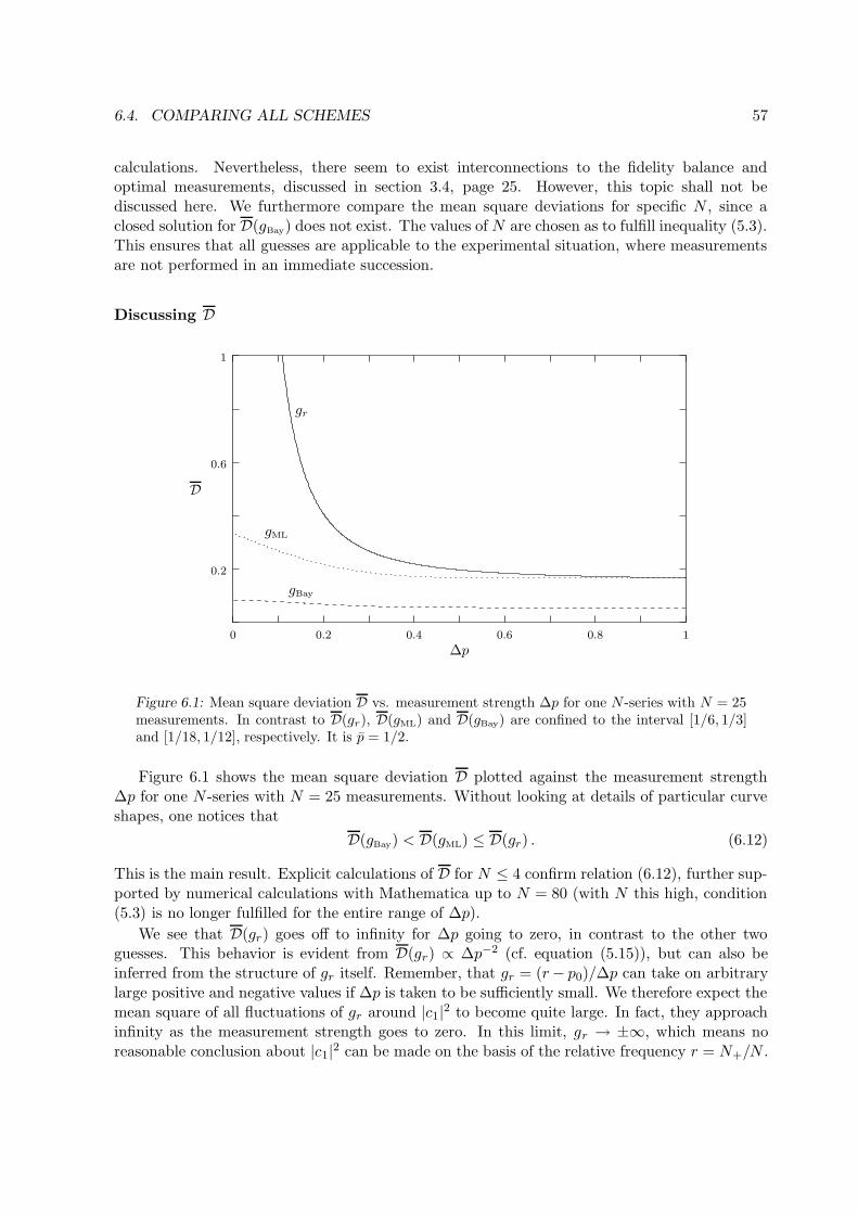
6.4. COMPARING ALL SCHEMES 57
calculations. Nevertheless, there seem to exist interconnections to the fidelity balance andoptimal measurements, discussed in section 3.4, page 25. However, this topic shall not bediscussed here. We furthermore compare the mean square deviations for specific N , since aclosed solution for D(gBay) does not exist. The values of N are chosen as to fulfill inequality (5.3).This ensures that all guesses are applicable to the experimental situation, where measurementsare not performed in an immediate succession.
Discussing D
gr
gML
gBay
0.2
0.6
1
0 0.2 0.4 0.6 0.8 1
D
∆p
Figure 6.1: Mean square deviation D vs. measurement strength ∆p for one N -series with N = 25measurements. In contrast to D(gr), D(gML) and D(gBay) are confined to the interval [1/6, 1/3]and [1/18, 1/12], respectively. It is p = 1/2.
Figure 6.1 shows the mean square deviation D plotted against the measurement strength∆p for one N -series with N = 25 measurements. Without looking at details of particular curveshapes, one notices that
D(gBay) < D(gML) ≤ D(gr) . (6.12)
This is the main result. Explicit calculations of D for N ≤ 4 confirm relation (6.12), further sup-ported by numerical calculations with Mathematica up to N = 80 (with N this high, condition(5.3) is no longer fulfilled for the entire range of ∆p).
We see that D(gr) goes off to infinity for ∆p going to zero, in contrast to the other twoguesses. This behavior is evident from D(gr) ∝ ∆p−2 (cf. equation (5.15)), but can also beinferred from the structure of gr itself. Remember, that gr = (r− p0)/∆p can take on arbitrarylarge positive and negative values if ∆p is taken to be sufficiently small. We therefore expect themean square of all fluctuations of gr around |c1|2 to become quite large. In fact, they approachinfinity as the measurement strength goes to zero. In this limit, gr → ±∞, which means noreasonable conclusion about |c1|2 can be made on the basis of the relative frequency r = N+/N .
58 CHAPTER 6. PARAMETER ESTIMATION
For fairly strong measurements, D(gr) clings to the horizontal asymptote Dprojective = 1/6.This behavior gets more pronounced the higher N , that is, D(gr) drops faster to Dprojective forsmaller ∆p. In the limit of infinitely many measurements,
limN→∞
D(gr) = Dprojective =1
6, (6.13)
independent of ∆p. This expresses the fact that an infinite series of unsharp measurements isequivalent to one projective measurement. See p. 58 of [Kon03] for a proof of this statement.
The maximum likelihood guess gML displays the same asymptotic behavior (6.13) for large∆p and high N . In contrast to D(gr), D(gML) is bounded above by
lim∆p→0
D(gML) =1
3,
verified numerically forN ≤ 30. This restriction of D(gML) over the whole range of measurementscan again be made clear by looking at gML itself. It is either 0 or 1, so fluctuations are boundto this interval, which implies a finite mean square deviation. Although gML seems a very crudeestimate in comparison to gr, we see that D(gML) always lies below D(gr), a somehow unexpectedresult.
The Bayesian estimator D(gBay) even lies below the maximum likelihood deviation, a con-sequence of the incorporated a priori information about |c1|2. Striking feature of D(gBay) is itssmall absolute value, lying in between 1/18 for projective measurements and 1/12 for ∆p = 0(analytically as well as numerically verified for N ≤ 30). In analogy to the finite deviationof gML, these small deviations can be attributed to the special behavior of gBay. A moment’sthought shows that gBay is restricted to the interval
1
3≤ gBay ≤ 2
3. (6.14)
This accounts for its low mean square deviation. In fact, gBay is the best possible estimate onecan make, taking D as the criterion. Recall, that we got gBay by minimizing the mean squareerror, averaged over the a posteriori distribution p(|c1|2
∣
∣N+) for |c1|2. Now, because of (6.11),the minimum of Dpost(gBay) is also the minimum for our criterion D: Assume we want to findthe guess g minimizing D, defined in (5.14). D(g) then reads
D(g) =
N∑
N+=0
∫ 1
0d|c1|2p(N+
∣
∣N, |c1|2)(g − |c1|2)2
=
N∑
N+=0
(
N
N+
)[
1
2(α0 + α1)g
2 +1
3(α0 + 2α1)g +
1
3α0 +
1
4(α1 − α0)
]
.
Solving for ∂D(g)/∂g = 0 yields g = gBay. Hence, there exists no estimate having a lower meansquare deviation D than gBay.
Remark: The POVMs corresponding to gBay = 1/3 respectively gBay = 2/3 describe phasedamping, cf. [Nie01], page 384. For example, if gBay = 2/3, then p0 = 0 and E+ = p1|1〉〈1|,E− = |0〉〈0| + (1 − p1)|1〉〈1|.
6.4. COMPARING ALL SCHEMES 59
Is D an Appropriate Measure?
Although gBay has the lowest possible deviation, it is an unbiased estimator, as can be seenfrom relation (6.14) (take, for example, |c1|2 = 0.8). This poses the question whether D isan appropriate measure to define the quality of a guess, if used in the context of real-timevisualization of dynamics. In this respect the mean square deviation competes with criterianormally used in parameter estimation theory (cf. Appendix C.2). gr is – by construction – anunbiased guess, which ensures the correct estimate (true value of |c1|2) in the limit of infinitelymany ensembles (of finite size). Nevertheless, D(gr) lies above D(gML) and D(gBay). gML doesnot seem to be unbiased, although this could not be verified analytically.
So far, a conclusive answer to what criterion is best used cannot be given. The classicalmeasures unbiasedness and efficiency are not applicable to the mean square deviation, since nomeasured average for |c1|2 exists. Consistency seems a reasonable criterion for a guess: Theerror made with a guess should go to zero if the ensemble size goes to infinity. Then, an infiniteamount of information would be available and the guess would be exact.
D defined in (5.14) was developed in close analogy to the classical measure variance. It thusrepresents a first step towards a measure suited to analyze the error made with a guess obtainedfrom an N -series. See [Kle03] for a thorough discussion.
Discussing DShould we find ourselves in the situation where more information about |c1|2 is available to usthan ‘equipartition within the unit interval’, the average over states is unnecessary. Then D isa sufficient measure to make statements about different guesses and their dependence on |c1|2.
Figure 6.2 shows the mean square deviation D versus measurement strength ∆p for N = 4measurements and different states |c1|2. The four plots display D(g) for the eigenstates |0〉 and|1〉 (|c1|2 = 0 and |c1|2 = 1, respectively) as well as two superpositions |ψ〉 = c0|0〉 + c1|1〉(|c1|2 = 0.3 and |c1|2 = 0.7). Except for the lower left plot, axes labels have been suppressed forbetter readability.
In contrast to figure 6.1, statements about the quality of a particular guess now depend onthe measurement strength as well as the state one is presupposing. For |c1|2 sufficiently awayfrom the corresponding eigenstates, we qualitatively recover the main result (6.12), now statedwith D instead of D:
D(gBay) < D(gML) ≤ D(gr) .
This is not surprising. Because gBay lies within the interval [1/3, 2/3], the estimate never liesfar away from the actual value of |c1|2. On the other hand, the maximum likelihood estimate iseither 0 or 1, so on average, gML lies further away from |c1|2 than gBay. Again, gr has the highestdeviation D, regardless of the applied measurement strength.
The situation changes if |c1|2 lies close to either one of the respective eigenstates |0〉 or |1〉.For strong measurements, gML and gr outrun the Bayesian estimate, because of its confinementto the interval [1/3, 2/3]. The maximum likelihood estimate is now almost perfectly well suitedto follow the evolution of |c1|2, as well as gr, whose deviation D(gr) drops to zero for projectivemeasurements, and |c1|2 = 0 or |c1|2 = 1.
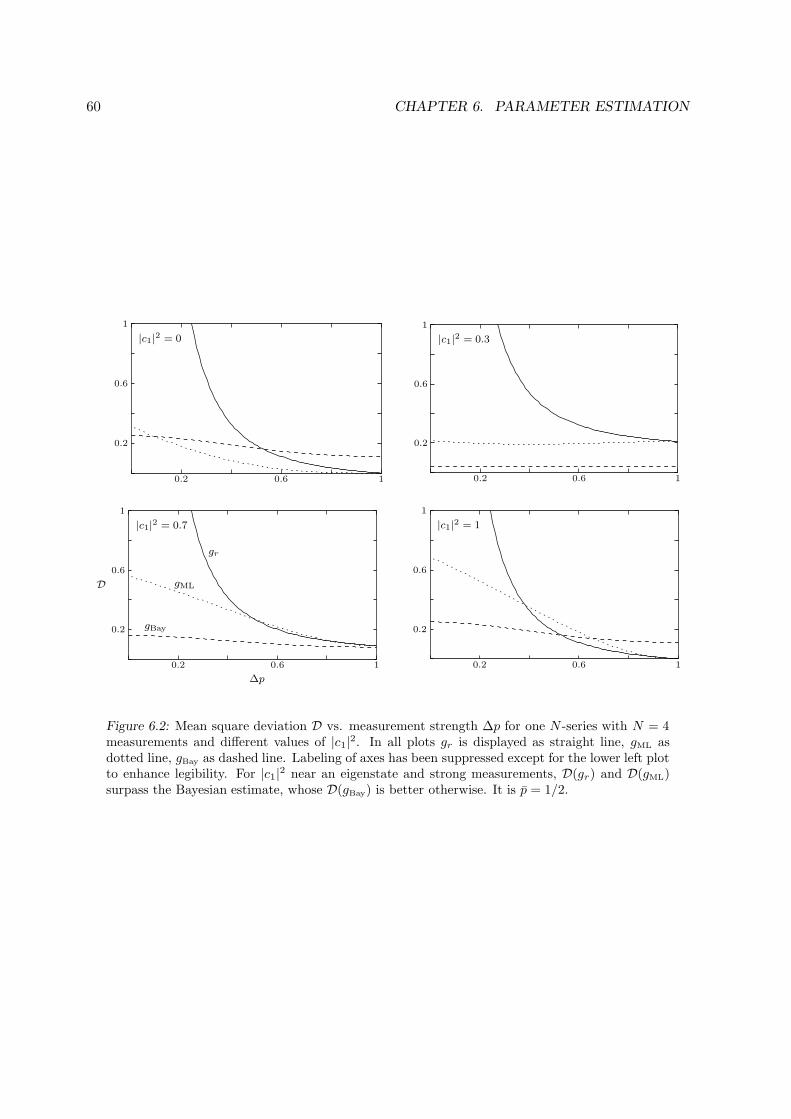
60 CHAPTER 6. PARAMETER ESTIMATION
|c1|2 = 0 |c1|2 = 0.3
|c1|2 = 1
D
gr
gML
gBay
∆p
|c1|2 = 0.7
0.2
0.6
1
0.2
0.6
0.2 0.6
0.2
0.6
1
0.2 0.6 1
0.2
0.6
1
0.2 0.6 10.60.2
1
1
1
Figure 6.2: Mean square deviation D vs. measurement strength ∆p for one N -series with N = 4measurements and different values of |c1|2. In all plots gr is displayed as straight line, gML asdotted line, gBay as dashed line. Labeling of axes has been suppressed except for the lower left plotto enhance legibility. For |c1|2 near an eigenstate and strong measurements, D(gr) and D(gML)surpass the Bayesian estimate, whose D(gBay) is better otherwise. It is p = 1/2.
Chapter 7
Summary and Outlook
7.1 Summary
Several aspects of state and parameter estimation in quantum theory have been studied in thiswork using the language of generalized measurements (POVM measurements).
In the first part, comprising chapters 3 and 4, the delicate balance between informationgained from a measurement and thereby induced state disturbance was investigated. For onemeasurement (mapping pure states to pure states) on a single system, the resulting trade-off [Ban01a] in terms of mean operation fidelities F and G was investigated for qubits and aspecial class of qubit POVMs. This special class consists of measurements with commutingeffects. Such unsharp measurements can be interpreted in terms of ordinary observables, as, forexample, energy or spin. The optimal balance between information gain and disturbance wasdetermined to be a simple constraint, restricting the parameters characterizing these unsharpmeasurements.
A clear visualization of the trade-off is provided by the FG-plane. Here, the trade-off couldbe expressed in terms of parameters characterizing the unsharp qubit POVM. This parametriza-tion revealed a simple structure, separating minimal from non-minimal measurements (Krausoperators of non-minimal measurements have a non-trivial unitary back-action term in their po-lar decomposition). Non-minimal measurements were found to deteriorate the optimal balancenoticeably.
If nothing is known a priori about the pure qubit state to be estimated, a unitary back-actionterm, i.e. non-minimal measurements, can not improve on the mean operation fidelity F . If, how-ever, a priori information about the qubit is available, then – as was shown in chapter 4 – asuitably chosen back-action improves on the mean operation fidelity, calculated for minimalmeasurements and a priori information. The latter fidelity, in turn, can be larger or smallerthan the mean operation fidelity calculated if no a priori information about the qubit exists;that is, information not necessarily implies a higher fidelity. Interestingly, the mean operationfidelity calculated for a priori information and non-minimal measurements, containing this spe-cial back-action, can be higher than the mean operation fidelity calculated if there is no a prioriinformation.
In the second part, comprising chapters 5 and 6, focus is shifted to the estimation of pa-rameters characterizing dynamics of a qubit. Building upon previous work on the real-timevisualization of a qubit’s Rabi oscillations which employs sequences of unsharp measurements
61
62 CHAPTER 7. SUMMARY AND OUTLOOK
(N -series), different estimation procedures were devised and compared. The originally proposedestimator [Aud01] was constructed to fulfill unbiasedness, a criterion used in classical estimationtheory. The second estimator (guess) developed uses the maximum likelihood method. It dis-cards, however, eventually available pre-measurement information about the qubit. The thirdguess (Bayesian estimator) takes this fact into account by means of Bayes’ theorem.
To compare all guesses, a mean square deviation was constructed to define a measure ofquality. With this measure at hand, it was shown that for one N -series, the Bayesian estimatoris superior to the maximum likelihood – as well as the original estimator. The latter, in turn, isinferior (i.e. has a larger mean square deviation) to the maximum likelihood estimator.
7.2 Outlook
The increase in fidelity by certain unitary back-actions and pre-measurement information aboutthe qubit state is an interesting and unexpected effect, requiring further investigation. In thisconnection, the distinguishability of two non-orthogonal pure states, quantifiable e.g. by theerror probability, poses an interesting problem. It would be worthwhile to check whether areduction of the error probability is possible by means of the special non-minimal measurementsintroduced in chapter 4.
Without information about the pre-measurement state, the fidelity trade-off between F andG is optimized for the special class of minimal measurements with commuting effects. Thequestion arises if these unsharp measurements are the only class saturating the optimal upperbound.
In chapter 6 the mean square deviation was used to compare all three estimators obtainedfrom the measurement results of one N -series. By definition, the measurements constitutingone N -series were carried out in an immediate succession. That is, no dynamical evolution ofthe state in between two measurements could take place. If dynamical processes are taken intoaccount, the question poses itself whether the mean square deviation is an appropriate measureany longer. Numerical simulations of the estimators derived in this work are currently made toelucidate things.
Appendix A
Calculations in Chapters 3 and 4
A.1 Inequalities Used for Trade-Off
In deriving the fidelity balance (3.15) between F and G we made use of two vector inequalitiesfrom linear algebra. I placed the omitted details in this appendix in order not to interrupt theflux of the presentation.
Cauchy-Schwarz Inequality
The Cauchy-Schwarz inequality states that for two arbitrary vectors x,y ∈ N the inequality
x · y ≤ |x| · |y| (A.1)
always holds, with equality being reached if and only if x = ay (a > 0). | · | denotes the usual2-norm. The proof of (A.1) can be found in every introductory textbook on linear algebra. Here,I only prove the equality sign: if x = ay with a > 0, we get
l.h.s = x · y = ay · y = ay2
r.h.s = |x| · |y| = a|y| · |y| = ay2 .
Inequality Between Quadratic and Arithmetic Mean
For a sequence of real numbers ai ∈ and N ∈ , the arithmetic mean mA and the quadraticmean mQ are defined through
mA :=1
N
N∑
i=1
ai and mQ :=
(
1
N
N∑
i=1
a2i
)1/2
,
with the inequality mA ≤ mQ ∀ai ∈ holding between them. Equality is reached if and only ifa1 = · · · = aN . To see this, we evaluate both sides of the inequality assuming ai = a ∀i:
l.h.s =1
N
N∑
i=1
a =1
NNa = a
r.h.s =
(
1
N
N∑
i=1
a2
)1/2
=
(
1
NNa2
)1/2
= a .
63
64 APPENDIX A. CALCULATIONS IN CHAPTERS 3 AND 4
A.2 Calculation of FΩ(Us
√Es)
A calculation becomes more error-prone the longer it gets. I therefore give the explicit derivationof FΩ(Us
√Es) in section 4.3 (p. 32), so that the reader should be able to reconstruct every step
of it.
Suppose we transformed our knowledge about the pre-measurement state |ψ〉 into a region Ωon the surface of the Bloch sphere. After choosing |ψ〉, we rotate Ω via the unitary transformationUz = exp iξσz, such that |ψ〉 lies in the yz-plane. Requiring the action of
√Es on |ψ〉 to be
fully compensated by Us = exp ±iαs/2σx determines the two angles αs by which every statewithin Ω will be rotated. αs are given by (4.3), the scalar product between the normed Blochvectors of |ψ〉 and |ψ〉.
We start with the definition (4.1):
FΩ(Us√
Es) =1
N(Ω)
∫
Ωdψ∑
s=±|〈ψ|Us
√
Es|ψ〉|2 .
Evaluation of the integral is not necessary for a qualitative analysis, so it suffices to calculatethe integrand,
∑
s=±|〈ψ|Us
√
Es|ψ〉|2 = |〈ψ| exp −iα+
2σx√
E+|ψ〉|2 + |〈ψ| exp iα−2σx√
E−|ψ〉|2 .
Both terms are calculated in the same fashion, so we focus on the term with α+. Using
exp ±iαs2σx = cos
αs2
± i sinαs2σx ,
we get
|〈ψ| exp −iα+
2σx√
E+|ψ〉|2 = |〈ψ|(
cosα+
2
− i sinα+
2σx)√
E+|ψ〉|2
= | cos α+
2〈ψ|√
E+|ψ〉 − i sinα+
2〈ψ|σx
√
E+|ψ〉|2
= cos2 α+
2|〈ψ|
√
E+|ψ〉|2 + sin2 α+
2|〈ψ|σx
√
E+|ψ〉|2
+i
2sinα+〈ψ|
√
E+|ψ〉(
〈ψ|σx√
E+|ψ〉∗ − 〈ψ|σx√
E+|ψ〉)
.
(A.2)
In the last step we used positivity1 of√E+ and 2 sin (α+/2) cos (α+/2) = sinα+. The Pauli
matrix σx = |0〉〈1| + |1〉〈0| is hermitian, 〈ψ|σx√E+|ψ〉∗ = 〈ψ|(σx
√E+)†|ψ〉 = 〈ψ|σx
√E+|ψ〉,
and (A.2) writes
|〈ψ| exp −iα+
2σx√
E+|ψ〉|2 = cos2 α+
2|〈ψ|
√
E+|ψ〉|2 + sin2 α+
2|〈ψ|σx
√
E+|ψ〉|2
+i
2sinα+〈ψ|
√
E+|ψ〉〈ψ|[√
E+, σx]|ψ〉 .
1The modulus in |〈ψ|√E+|ψ〉|2 can be omitted. We will leave it for optical homogeneity, though.
A.2. CALCULATION OF FΩ(US√ES) 65
With the commutator [√E+, σx] = i(
√p0 −
√p1)σy, we finally arrive at
|〈ψ| exp −iα+
2σx√
E+|ψ〉|2 = cos2α+
2|〈ψ|
√
E+|ψ〉|2 + sin2 α+
2|〈ψ|σx
√
E+|ψ〉|2
+1
2(√p1 −
√p0)〈ψ|
√
E+|ψ〉〈ψ|σy |ψ〉 sinα+ . (A.3)
Similarly, the second term with α− is evaluated along the same line. One gets
|〈ψ| exp iα−2σx√
E−|ψ〉|2 = cos2α−2
|〈ψ|√
E−|ψ〉|2 + sin2 α−2
|〈ψ|σx√
E−|ψ〉|2
+1
2(√
1 − p0 −√
1 − p1)〈ψ|√
E−|ψ〉〈ψ|σy |ψ〉 sinα− . (A.4)
With (A.3) and (A.4), FΩ(Us√Es) reads
FΩ(Us√
Es) =1
N(Ω)
∫
Ωdψ
∑
s=±|〈ψ|
√
Es|ψ〉|2 cos2 αs2
+ |〈ψ|σx√
Es|ψ〉|2 sin2 αs2
+1
2〈ψ|σy|ψ〉
[
(√p1 −
√p0)〈ψ|
√
E+|ψ〉 sinα+ + (√
1 − p0 −√
1 − p1)〈ψ|√
E−|ψ〉 sinα−]
.
To connect FΩ(√Es) to FΩ(Us
√Es), the final substitution cos2 (αs/2) = 1− sin2 (αs/2) is made
which leads to the result (4.4) with minimal term (4.6) and difference term (4.9).

66 APPENDIX A. CALCULATIONS IN CHAPTERS 3 AND 4
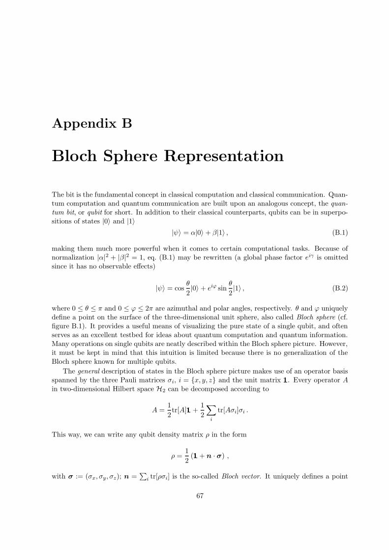
Appendix B
Bloch Sphere Representation
The bit is the fundamental concept in classical computation and classical communication. Quan-tum computation and quantum communication are built upon an analogous concept, the quan-tum bit, or qubit for short. In addition to their classical counterparts, qubits can be in superpo-sitions of states |0〉 and |1〉
|ψ〉 = α|0〉 + β|1〉 , (B.1)
making them much more powerful when it comes to certain computational tasks. Because ofnormalization |α|2 + |β|2 = 1, eq. (B.1) may be rewritten (a global phase factor eiγ is omittedsince it has no observable effects)
|ψ〉 = cosθ
2|0〉 + eiϕ sin
θ
2|1〉 , (B.2)
where 0 ≤ θ ≤ π and 0 ≤ ϕ ≤ 2π are azimuthal and polar angles, respectively. θ and ϕ uniquelydefine a point on the surface of the three-dimensional unit sphere, also called Bloch sphere (cf.figure B.1). It provides a useful means of visualizing the pure state of a single qubit, and oftenserves as an excellent testbed for ideas about quantum computation and quantum information.Many operations on single qubits are neatly described within the Bloch sphere picture. However,it must be kept in mind that this intuition is limited because there is no generalization of theBloch sphere known for multiple qubits.
The general description of states in the Bloch sphere picture makes use of an operator basisspanned by the three Pauli matrices σi, i = x, y, z and the unit matrix
. Every operator A
in two-dimensional Hilbert space H2 can be decomposed according to
A =1
2tr[A]
+
1
2
∑
i
tr[Aσi]σi .
This way, we can write any qubit density matrix ρ in the form
ρ =1
2(
+ n · σ) ,
with σ := (σx, σy, σz); n =∑
i tr[ρσi] is the so-called Bloch vector. It uniquely defines a point
67
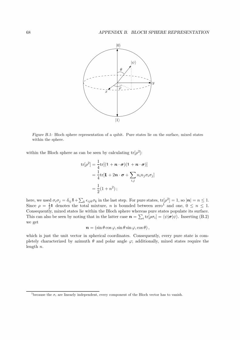
68 APPENDIX B. BLOCH SPHERE REPRESENTATION
θ
|ψ〉
ϕy
x
|0〉
|1〉
Figure B.1: Bloch sphere representation of a qubit. Pure states lie on the surface, mixed stateswithin the sphere.
within the Bloch sphere as can be seen by calculating tr[ρ2]:
tr[ρ2] =1
4tr[(
+ n · σ)(
+ n · σ)]
=1
4tr[
+ 2n · σ +
∑
i,j
ninjσiσj ]
=1
2(1 + n2) ;
here, we used σiσj = δij+∑
k εijkσk in the last step. For pure states, tr[ρ2] = 1, so |n| = n ≤ 1.Since ρ = 1
2
denotes the total mixture, n is bounded between zero1 and one, 0 ≤ n ≤ 1.
Consequently, mixed states lie within the Bloch sphere whereas pure states populate its surface.This can also be seen by noting that in the latter case n =
∑
i tr[ρσi] = 〈ψ|σ|ψ〉. Inserting (B.2)we get
n = (sin θ cosϕ, sin θ sinϕ, cos θ) ,
which is just the unit vector in spherical coordinates. Consequently, every pure state is com-pletely characterized by azimuth θ and polar angle ϕ; additionally, mixed states require thelength n.
1because the σi are linearly independent, every component of the Bloch vector has to vanish.
Appendix C
Notes on Probability Theory
Basics of probability theory can be found in every introductory textbook on the subject, e.g.[Lar83] and [Kre70]. Therefore this appendix should not be viewed as a thorough introductionbut rather as a convenience to the reader. We assume a certain familiarity with elementary settheory, since it provides a clear and exact language for stating and solving probability problems.
Part one reviews some basic definitions and results given in [Nie01], whereas part two providesdefinitions of quality measures for estimators.
C.1 Basics
The basic notion of probability theory is that of a random variable. A random variable X maytake one of a number of values, x, with probability pX(x). We use upper case to denote therandom variable, and x to denote the values that random variable may take. All possible valuesare elements of some sample space Ω which can be continuous or discrete. In this thesis we areonly concerned with discrete sample spaces, i.e. any random variable can take values from afinite (or countably infinite) set of values.
A probability function pX of some random variable X assigns a real number to any elementor subset of the sample space of X. From intuition it is clear what properties such a probabilityfunction must have: probabilities always have to be positive and add up to one, since one eventalways happens in any experiment. The third property a probability measure should satisfy isthat of additivity: if two events are independent (i.e. every outcome of an experiment dependsin no way on any other outcome), their respective probabilities of occurrence should add up.A strict formulation of these intuitive rules in abstract probability theory was first given byKolmogorov [Kol33]:
Definition C.1 (probability axioms). A probability function pX of a random variable X isa real-valued set function defined on the class of all subsets Σ of the sample space Ω and has tofulfill the following three rules:
(i) pX(Ω) = 1
(ii) pX(Σ) ≥ 0 for all Σ ⊂ Ω
(iii) pX(Σ1 ∪ Σ2 ∪ · · · ) = pX(Σ1) + pX(Σ2) + · · · if Σi ∩ Σj = ∅ ∀ i 6= j.
69
70 APPENDIX C. NOTES ON PROBABILITY THEORY
In experiments, one often has to consider two random variables X and Y (if no ambiguitiesarise, the subscripts on p are dropped in the following). The conditional probability that Y = ygiven that X = x is defined by
p(y∣
∣x) :=p(x ∩ y)p(x)
, (C.1)
where p(x ∩ y) is the probability that X = x and Y = y. When p(x) = 0 the conventionp(y∣
∣x) = 0 is made. For independent random variables X and Y , p(x ∩ y) = p(x)p(y) for all xand y; additionally, one has p(y
∣
∣x) = p(y) for all x and y.Bayes’ theorem relates the conditional probabilities for Y given X to those for X given Y ,
p(x∣
∣y) = p(y∣
∣x)p(x)
p(y); (C.2)
it is a direct consequence of (C.1), since p(x ∩ y) = p(y ∩ x). The probability p(y) appearing in(C.2) is often re-expressed using the law of total probability. It states that if X and Y are tworandom variables, then the probabilities for Y can be expressed in terms of the probabilities forX, and the conditional probabilities for Y given X,
p(y) =∑
x
p(y∣
∣x)p(x) ,
where the sum is over all values x of the respective sample space. The expectation, average ormean of a random variable X is defined by
〈X〉 :=∑
x
p(x)x .
〈·〉 is a linear function; for independent X and Y , 〈XY 〉 = 〈X〉〈Y 〉. The variance of a randomvariable X is defined by the expression
σ2(X) := 〈(X − 〈X〉)2〉 = 〈X2〉 − 〈X〉2 .
Its square root σ(X) :=√
σ2(X), called standard deviation, is a measure of the spread of arandom variable about the average.
C.2 Properties of Estimators
One problem of statistical inference is that of estimating one or more unknown parameters u ofsome probability distribution pX(u) for the random variable X. Here we shall not be concernedwith methods of how to find a guess (called ‘estimator’) u(x1, . . . , xN ) given a sample of size N .Instead we will review three criteria judging the quality of a given estimator u.
Definition C.2 (unbiasedness). An estimator u of an unknown parameter u is unbiased if〈u〉 = u.
Thus, an unbiased estimator is a random variable whose expected value is the parameterbeing estimated; if we were to take samples of size N repeatedly and for each compute theobserved value of u (the estimate for that sample outcome), then the average of these observedvalues would be u, the parameter being estimated.
C.2. PROPERTIES OF ESTIMATORS 71
The property of unbiasedness ensures that the estimator u yields the true value of theparameter u in the limit of infinite ensembles. However, this statement does not imply thatthe estimator has very high probability of lying close to the unknown parameter for any givenensemble. Suppose we have two unbiased estimators u1, u2 for the same sample. Clearly, wewould take the estimator who has the higher probability of lying close to the parameter. Thisleads us to consider the variances of unbiased estimators:
Definition C.3 (efficiency). If u1 and u2 are both unbiased estimators of u for the samesample, then u1 is more efficient than u2 if
σ2(u1) < σ2(u2) .
There is one further property which estimators may possess, that of consistency:
Definition C.4 (consistency). u is a consistent estimator of u if
limN→∞
[p(u− u) < ε] = 1 for any ε > 0
(N is the sample size).
Note first of all that an estimator u is consistent if a sequence of probabilities (evaluatedfrom the probability distribution of u) converges to one as the sample size increases. Thusconsistency, strictly speaking, has to do only with the limiting behavior of an estimator as thesample size increases without limit and does not imply that the observed value of u is necessarilyclose to u for any specific sample size N (cf. efficiency). This is not the same as unbiasedness,where only different ensembles of fixed size N are considered.
There is a theorem (cf. page 233 of [Lar83]) which gives a relatively easy check on whether aparticular estimator is consistent. It says that if u is a random variable whose value gets closerand closer to u as N increases, and whose variance shrinks to zero as N increases, it will be aconsistent estimator of u.

72 APPENDIX C. NOTES ON PROBABILITY THEORY
Bibliography
[Aci00] A. Acin, J. I. Latorre and P. Pascual. Optimal generalized quantum measurements forarbitrary spin systems. Phys. Rev. A 61 (2000) 022113.
[Aud01] J. Audretsch, T. Konrad and A. Scherer. A sequence of unsharp measurements en-abling a real-time visualization of a quantum oscillation. Phys. Rev. A 63 (2001)052102.
[Aud02a] J. Audretsch, L. Diosi and T. Konrad. Estimating the post-measurement state. quant-ph (2002) 0210205.
[Aud02b] J. Audretsch, L. Diosi and T. Konrad. Evolution of a qubit under the influence ofa sucession of weak measurements with unitary feedback. Phys. Rev. A 66 (2002)022310.
[Aud02c] J. Audretsch, T. Konrad and A. Scherer. Quantum-optical weak measurements canvisualize photon dynamics in real time. Phys. Rev. A 65 (2002) 033814.
[Bag02] E. Bagan, M. Baig and R. Munoz-Tapia. Optimal scheme for estimating a pure qubitstate via local measurements. quant-ph:0205026v2 (2002).
[Ban00] K. Banaszek. Optimal quantum teleportation with an arbitrary pure state. Phys. Rev.A 62 (2000) 024301.
[Ban01a] K. Banaszek. Fidelity Balance in Quantum Operations. Phys. Rev. Lett. 86 (2001)1366.
[Ban01b] K. Banaszek and I. Devetak. Fidelity trade-off for finite ensembles of identicallyprepared qubits. Phys. Rev. A 64 (2001) 052307.
[Bru99] D. Bruß and C. Macchiavello. Optimal state estimation for d-dimensional quantumsystems. Physics Letters A 253 (1999) 249.
[Bus91] P. Busch, P. J. Lahti and P. Mittelstaedt. The Quantum Theory of Measurement.Springer-Verlag Berlin (1991).
[Bus95] P. Busch, M. Grabowski and P. J. Lahti. Operational Quantum Physics. LectureNotes in Physics. Springer-Verlag (1995).
[Der98] R. Derka, V. Buzek and A. K. Ekert. Universal Algorithm for Optimal Estimationof Quantum States from Finite Ensembles via Realizable Generalized Measurement.Phys. Rev. Lett. 80 (1998) 1571.
73
74 BIBLIOGRAPHY
[Fis00] D. G. Fischer, S. H. Kienle and M. Freyberger. Quantum-state estimation by self-learning measurements. Phys. Rev. A 61 (2000) 032306.
[Fuc95] Christopher A. Fuchs. Distinguishability and Accessible Information in Quantum The-ory. Dissertation Center for Advanced Studies, Department of Physics and Astronomy,University of New Mexico Albuquerque, NM 87131-1156 (1995).
[Han02] Th. Hannemann, D. Reiss, Ch. Balzer, W. Neuhauser, P. E. Toschek and Ch. Wun-derlich. Self-learning estimation of quantum states. Phys. Rev. A 65 (2002) 050303.
[Hol82] A. S. Holevo. Probabilistic and Statistical Aspects of Quantum Theory. North-HollandAmsterdam (1982).
[Kle03] F. E. Klee. Sequential Measurements. Diplomarbeit Universitat Konstanz (2003). Inpreparation.
[Kol33] A. Kolmogoroff. Grundbegriffe der Wahrscheinlichkeitsrechnung. Springer-VerlagBerlin (1933).
[Kon03] T. Konrad. Less is More: On the Theory and Application of Weak and Unsharp Mea-surements in Quantum Mechanics. Dissertation Universitat Konstanz, Marz (2003).
[Kra83] K. Kraus. States, Effects and Operations. Springer-Verlag Berlin (1983).
[Kre70] E. Kreyszig. Statistische Methoden und ihre Anwendungen. Vandenhoek & RuprechtGottingen, Germany (1970).
[Lar83] H. J. Larson. Introduction to Probability Theory and Statistical Inference. J. Wiley &Sons third edition (1983).
[Lat98] J. I. Latorre, P. Pascual and R. Tarrach. Minimal Optimal Generalized QuantumMeasurements. Phys. Rev. Lett. 81 (1998) 1351.
[Mas95] S. Massar and S.Popescu. Optimal Extraction of Information from Finite QuantumEnsembles. Phys. Rev. Lett. 74 (1995) 1259.
[Nie01] Michael A. Nielsen and Isaac L. Chuang. Quantum Computation and Quantum In-formation. Cambridge University Press (2001).
[Pau33] W. Pauli. Die allgemeinen Prinzipien der Wellenmechanik. Springer-Verlag Berlin(1933).
[Per89] A. Peres. Quantum limited detectors for weak classical signals. Phys. Rev. D 39(1989) 2943.
[Per91] A. Peres and W. K. Wootters. Optimal Detection of Quantum Information. Phys.Rev. Lett. 66 (1991) 1119.
[Per93] A. Peres. Quantum Theory: Concepts and Methods. Kluwer Academic Publishers(1993).
BIBLIOGRAPHY 75
[Sch94] R. Schack, G. M. D’Ariano and C. M. Caves. Hypersensitivity to perturbation in thequantum kicked top. Phys. Rev. E 50 (1994) 972.
[Vid99] G. Vidal, J. I. Latorre, P. Pascual and R. Tarrach. Optimal minimal measurementsof mixed states. Phys. Rev. A 60 (1999) 126.
[vN32] J. von Neumann. Mathematische Grundlagen der Quantenmechanik. Springer-VerlagBerlin (1932).
[Wis95] H. M. Wiseman. Using feedback to eliminate back-action in quantum measurements.Phys. Rev. A 51 (1995) 2459.
[Woo82] W. K. Wootters and W. H. Zurek. A single quantum cannot be cloned. Nature 299(1982) 802.

76 BIBLIOGRAPHY
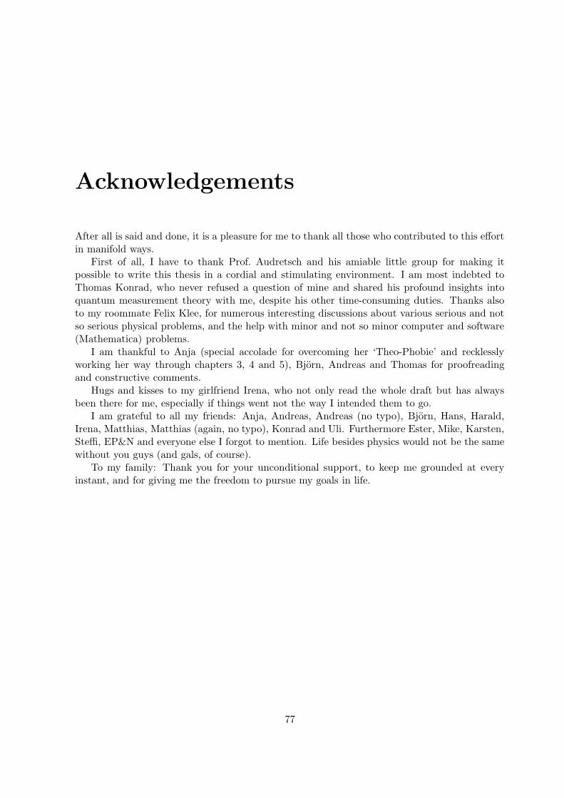
Acknowledgements
After all is said and done, it is a pleasure for me to thank all those who contributed to this effortin manifold ways.
First of all, I have to thank Prof. Audretsch and his amiable little group for making itpossible to write this thesis in a cordial and stimulating environment. I am most indebted toThomas Konrad, who never refused a question of mine and shared his profound insights intoquantum measurement theory with me, despite his other time-consuming duties. Thanks alsoto my roommate Felix Klee, for numerous interesting discussions about various serious and notso serious physical problems, and the help with minor and not so minor computer and software(Mathematica) problems.
I am thankful to Anja (special accolade for overcoming her ‘Theo-Phobie’ and recklesslyworking her way through chapters 3, 4 and 5), Bjorn, Andreas and Thomas for proofreadingand constructive comments.
Hugs and kisses to my girlfriend Irena, who not only read the whole draft but has alwaysbeen there for me, especially if things went not the way I intended them to go.
I am grateful to all my friends: Anja, Andreas, Andreas (no typo), Bjorn, Hans, Harald,Irena, Matthias, Matthias (again, no typo), Konrad and Uli. Furthermore Ester, Mike, Karsten,Steffi, EP&N and everyone else I forgot to mention. Life besides physics would not be the samewithout you guys (and gals, of course).
To my family: Thank you for your unconditional support, to keep me grounded at everyinstant, and for giving me the freedom to pursue my goals in life.
77