State and Output Feedback

Chapter 5

State and Output Feedback

This chapter describes how feedback can be used shape the local behaviorof a system. Both state and output feedback are discussed. The conceptsof reachability and observability are introduced and it is shown how statescan be estimated from measurements of the input and the output.

5.1 Introduction

The idea of using feedback to shape the dynamic behavior was discussed inbroad terms in Section 1.4. In this chapter we will discuss this in detail forlinear systems. In particular it will be shown that under certain conditions itis possible to assign the system eigenvalues to arbitrary values by feedback,allowing us to “design” the dynamics of the system.

The state of a dynamical system is a collection of variables that permitsprediction of the future development of a system. In this chapter we willexplore the idea of controlling a system through feedback of the state. Wewill assume that the system to be controlled is described by a linear statemodel and has a single input (for simplicity). The feedback control will bedeveloped step by step using one single idea: the positioning of closed loopeigenvalues in desired locations. It turns out that the controller has a veryinteresting structure that applies to many design methods. This chaptermay therefore be viewed as a prototype of many analytical design methods.

If the state of a system is not available for direct measurement, it isoften possible to determine the state by reasoning about the state throughour knowledge of the dynamics and more limited measurements. This isdone by building an “observer” that uses measurements of the inputs andoutputs of a linear system, along with a model of the system dynamics, to

109

110 CHAPTER 5. STATE AND OUTPUT FEEDBACK

estimate the state.

The details of the analysis and designs in this chapter are carried out forsystems with one input and one output, but it turns out that the structureof the controller and the forms of the equations are exactly the same forsystems with many inputs and many outputs. There are also many otherdesign techniques that give controllers with the same structure. A charac-teristic feature of a controller with state feedback and an observer is thatthe complexity of the controller is given by the complexity of the systemto be controlled. Thus the controller actually contains a model of the sys-tem. This is an example of the internal model principle which says that acontroller should have an internal model of the controlled system.

5.2 Reachability

We begin by disregarding the output measurements and focus on the evolu-tion of the state which is given by

dx

dt= Ax+Bu, (5.1)

where x ∈ Rn, u ∈ R, A is an n × n matrix and B an n × 1 matrix. A

fundamental question is if it is possible to find control signals so that anypoint in the state space can be reached.

First observe that possible equilibria for constant controls are given by

Ax+ bu0 = 0

This means that possible equilibria lies in a one (or possibly higher) dimen-sional subspace. If the matrix A is invertible this subspace is spanned byA−1B.

Even if possible equilibria lie in a one dimensional subspace it may stillbe possible to reach all points in the state space transiently. To explorethis we will first give a heuristic argument based on formal calculations withimpulse functions. When the initial state is zero the response of the stateto a unit step in the input is given by

x(t) =

∫ t

0eA(t−τ)Bdτ. (5.2)

The derivative of a unit step function is the impulse function δ(t), whichmay be regarded as a function which is zero everywhere except at the origin

5.2. REACHABILITY 111

and with the property that

∫ ∞

∞δ(t)dt = 1.

The response of the system to a impulse function is thus the derivative of(5.2)

dx

dt= eAtB.

Similarly we find that the response to the derivative of a impulse functionis

d2x

dt2= AeAtB.

The input

u(t) = α1δ(t) + α2δ(t) + αδ(t) + · · · + αnδ(n−1)(t)

thus gives the state

x(t) = α1eAtB + α2Ae

AtB + α3A2eAtB + · · · + αnA

n−1eAtB.

Hence, right after the initial time t = 0, denoted t = 0+, we have

x(0+) = α1B + α2AB + α3A2B + · · · + αnA

n−1B

The right hand is a linear combination of the columns of the matrix

Wr =[

B AB . . . An−1B]

. (5.3)

To reach an arbitrary point in the state space we thus require that there aren linear independent columns of the matrix Wc. The matrix is called thereachability matrix.

An input consisting of a sum of impulse functions and their derivativesis a very violent signal. To see that an arbitrary point can be reached withsmoother signals we can also argue as follow. Assuming that the initialcondition is zero, the state of a linear system is given by

x(t) =

∫ t

0eA(t−τ)Bu(τ)dτ =

∫ t

0eAτBu(t− τ)dτ.

It follows from the theory of matrix functions that

eAτ = Iα0(τ) +Aα1(τ) + . . .+An−1αn−1(τ)


and we find that

x(t) = B

∫ t

0α0(τ)u(t− τ) dτ +AB

∫ t

0α1(τ)u(t− τ) dτ+

. . .+An−1B

∫ t

0αn−1(τ)u(t− τ) dτ.

Again we observe that the right hand side is a linear combination of thecolumns of the reachability matrix Wr given by (5.3).

We illustrate by two examples.

Example 5.1 (Reachability of the Inverted Pendulum). Consider the invertedpendulum example introduced in Example 3.5. The nonlinear equations ofmotion are given in equation (3.5)

dx

dt=

[

x2

sinx1 + u cosx1

]

y = x1.

Linearizing this system about x = 0, the linearized model becomes

dx

dt=

[

0 11 0

]

x+

[

01

]

u

y =[

1 0]

x.

(5.4)

The dynamics matrix and the control matrix are

A =

[

0 11 0

]

, B =

[

01

]

The reachability matrix is

Wr =

[

0 11 0

]

. (5.5)

This matrix has full rank and we can conclude that the system is reachable.This implies that we can move the system from any initial state to any finalstate and, in particular, that we can always find an input to bring the systemfrom an initial state to the equilibrium.

Example 5.2 (System in Reachable Canonical Form). Next we will considera system by in reachable canonical form:

dz

dt=

−a1 −a2 . . . an−1 −an

1 0 0 00 1 0 0...0 0 1 0

z +

100...0

u = Az + Bu

5.2. REACHABILITY 113

To show that Wr is full rank, we show that the inverse of the reachabilitymatrix exists and is given by

W−1r =

1 a1 a2 . . . an

0 1 a1 . . . an−1...0 0 0 . . . 1

(5.6)

To show this we consider the product

[

B AB · · · An−1B]

W−1r =

[

w0 w1 · · · wn−1

]

where

w0 = B

w1 = a1B + AB

...

wn−1 = an−1B + an−2AB + · · · + An−1B.

The vectors wk satisfy the relation

wk = ak + wk−1

and iterating this relation we find that

[

w0 w1 · · · wn−1

]

=

1 0 0 . . . 00 1 0 . . . 0...0 0 0 . . . 1

which shows that the matrix (5.6) is indeed the inverse of Wr.

Systems That Are Not Reachable

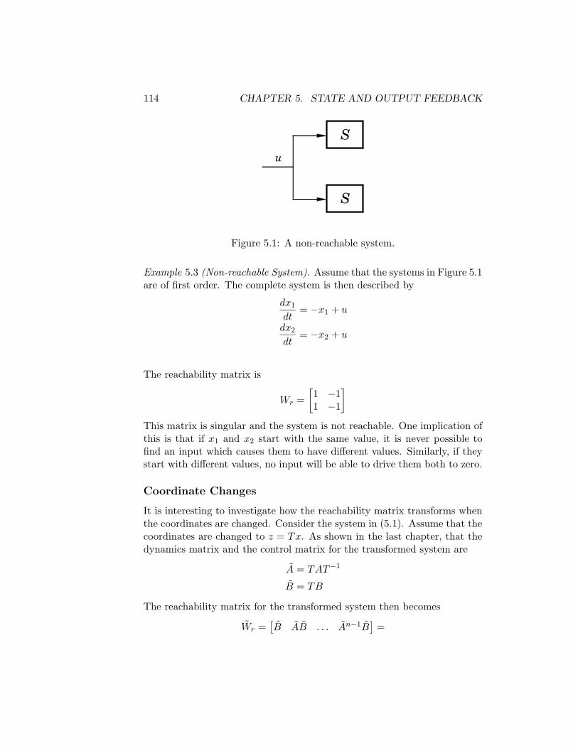
It is useful of have an intuitive understanding of the mechanisms that makea system unreachable. An example of such a system is given in Figure 5.1.The system consists of two identical systems with the same input. Theintuition can also be demonstrated analytically. We demonstrate this by asimple example.


u

S

S

Figure 5.1: A non-reachable system.

Example 5.3 (Non-reachable System). Assume that the systems in Figure 5.1are of first order. The complete system is then described by

dx1

dt= −x1 + u

dx2

dt= −x2 + u

The reachability matrix is

Wr =

[

1 −11 −1

]

This matrix is singular and the system is not reachable. One implication ofthis is that if x1 and x2 start with the same value, it is never possible tofind an input which causes them to have different values. Similarly, if theystart with different values, no input will be able to drive them both to zero.

Coordinate Changes

It is interesting to investigate how the reachability matrix transforms whenthe coordinates are changed. Consider the system in (5.1). Assume that thecoordinates are changed to z = Tx. As shown in the last chapter, that thedynamics matrix and the control matrix for the transformed system are

A = TAT−1

B = TB

The reachability matrix for the transformed system then becomes

Wr =[

B AB . . . An−1B]

=

5.3. STATE FEEDBACK 115

We have

AB = TAT−1TB = TAB

A2B = (TAT−1)2TB = TAT−1TAT−1TB = TA2B

...

AnB = TAnB.

The reachability matrix for the transformed system is thus

Wr =[

B AB . . . An−1B]

= T[

B AB . . . An−1B]

= TWr (5.7)

This formula is useful for finding the transformation matrix T that convertsa system into reachable canonical form (using Wr from Example 5.2).

5.3 State Feedback

Consider a system described by the linear differential equation

dx

dt= Ax+Bu

y = Cx(5.8)

The output is the variable that we are interested in controlling. To beginwith it is assumed that all components of the state vector are measured.Since the state at time t contains all information necessary to predict thefuture behavior of the system, the most general time invariant control lawis function of the state, i.e.

u(t) = f(x(t))

If the feedback is restricted to be a linear, it can be written as

u = −Kx+Krr (5.9)

where r is the reference value. The negative sign is simply a conventionto indicate that negative feedback is the normal situation. The closed loopsystem obtained when the feedback (5.8) is applied to the system (5.9) isgiven by

dx

dt= (A−BK)x+BKrr (5.10)


It will be attempted to determine the feedback gain K so that the closedloop system has the characteristic polynomial

p(s) = sn + p1sn−1 + . . .+ pn−1s+ pn (5.11)

This control problem is called the eigenvalue assignment problem or the poleplacement problem (we will define “poles” more formally in a later chapter).

Examples

We will start by considering a few examples that give insight into the natureof the problem.

Example 5.4 (The Double Integrator). The double integrator is described by

dx

dt=

[

0 10 0

]

x+

[

01

]

u

y =[

1 0]

x

Introducing the feedback

u = −k1x1 − k2x2 +Krr

the closed loop system becomes

dx

dt=

[

0 1−k1 −k2

]

x+

[

0Kr

]

r

y =[

1 0]

x

(5.12)

The closed loop system has the characteristic polynomial

det

[

s −1k1 s+ k2

]

= s2 + k2s+ k1

Assume it is desired to have a feedback that gives a closed loop system withthe characteristic polynomial

p(s) = s2 + 2ζω0s+ ω20

Comparing this with the characteristic polynomial of the closed loop systemwe find find that the feedback gains should be chosen as

k1 = ω20, k2 = 2ζω0

To have unit steady state gain the parameter Kr must be equal to k1 =ω2

0. The control law can thus be written as

u = k1(r − x1) − k2x2 = ω20(r − x1) − 2ζ0ω0x2


In the next example we will encounter some difficulties.

Example 5.5 (An Unreachable System). Consider the system

dx

dt=

[

0 10 0

]

x+

[

10

]

u

y = Cx =[

1 0]

x

with the control lawu = −k1x1 − k2x2 +Krr

The closed loop system is

dx

dt=

[

−k1 1 − k2

0 0

]

x+

[

Kr

0

]

r

This system has the characteristic polynomial

det

[

s+ k1 −1 + k2

0 s

]

= s2 + k1s = s(s+ k1)

This polynomial has zeros at s = 0 and s = −k1. One closed loop eigenvalueis thus always equal to s = 0 and it is not possible to obtain an arbitrarycharacteristic polynomial.

This example shows that the eigenvalue placement problem cannot al-ways be solved. An analysis of the equation describing the system showsthat the state x2 is not reachable. It is thus clear that some conditions onthe system are required.

The reachable canonical form has the property that the parameters ofthe system are the coefficients of the characteristic equation. It is thereforenatural to consider systems on this form when solving the eigenvalue place-ment problem. In the next example we investigate the case when the systemis in reachable canonical form.

Example 5.6 (System in Reachable Canonical Form). Consider a system inreachable canonical form, i.e,

dz

dt= Az + Bu =

−a1 −a2 . . . −an−1 −an

1 0 . . . 0 00 1 . . . 0 0...0 0 . . . 1 0

z +

100...0

u

y = Cz =[

b1 b2 · · · bn]

z.

(5.13)


The open loop system has the characteristic polynomial

Dn(s) = det

s+ a1 a2 . . . an−1 an

−1 s 0 00 −1 0 0...0 0 −1 s

.

Expanding the determinant by the last row we find that the following re-cursive equation for the determinant:

Dn(s) = sDn−1(s) + an.

It follows from this equation that

Dn(s) = sn + a1sn−1 + . . .+ an−1s+ an

A useful property of the system described by (5.13) is thus that the coef-ficients of the characteristic polynomial appear in the first row. Since theall elements of the B-matrix except the first row are zero it follows that thestate feedback only changes the first row of the A-matrix. It is thus straightforward to see how the closed loop eigenvalues are changed by the feedback.Introduce the control law

u = −Kz +Krr = −k1z1 − k2z2 − . . .− knzn +Krr (5.14)

The closed loop system then becomes

dz

dt=

−a1 − k1 −a2 − k2 . . . −an−1 − kn−1 −an − kn

1 0 0 00 1 0 0...0 0 1 0

z +

Kr

00...0

r

y =[

b1 b2 · · · bn]

z(5.15)

The feedback thus changes the elements of the first row of the A matrix,which corresponds to the parameters of the characteristic equation. Theclosed loop system thus has the characteristic polynomial

sn + (al + k1)sn−1 + (a2 + k2)s

n−2 + . . .+ (an−1 + kn−1)s+ an + kn


Requiring this polynomial to be equal to the desired closed loop polynomial(5.11) we find that the controller gains should be chosen as

k1 = p1 − a1

k2 = p2 − a2

...

kn = pn − an

This feedback simply replace the parameters ai in the system (5.15) by pi.The feedback gain for a system in reachable canonical form is thus

K =[

p1 − a1 p2 − a2 · · · pn − an

]

(5.16)

To have unit steady state gain the parameter Kr should be chosen as

Kr =an + kn

bn=pn

bn(5.17)

Notice that it is essential to know the precise values of parameters an andbn in order to obtain the correct steady state gain. The steady state gain isthus obtained by precise calibration. This is very different from obtainingthe correct steady state value by integral action, which we shall see in laterchapters. We thus find that it is easy to solve the eigenvalue placementproblem when the system has the structure given by (5.13).

The General Case

To solve the problem in the general case, we simply change coordinates sothat the system is in reachable canonical form. Consider the system (5.8).Change the coordinates by a linear transformation

z = Tx

so that the transformed system is in reachable canonical form (5.13). Forsuch a system the feedback is given by (5.14) where the coefficients are givenby (5.16). Transforming back to the original coordinates gives the feedback

u = −Kz +Krr = −KTx+Krr

It now remains to find the transformation. To do this we observe that thereachability matrices have the property

Wr =[

B AB . . . An−1B]

= T[

B AB . . . An−1B]

= TWr


The transformation matrix is thus given by

T = WrW−1r (5.18)

and the feedback gain can be written as

K = KT = KWrW−1r (5.19)

Notice that the matrix Wr is given by (5.6). The feedforward gain Kr isgiven by equation (5.17).

The results obtained can be summarized as follows.

Theorem 5.1 (Pole-placement by State Feedback). Consider the system givenby equation (5.8)

dx

dt= Ax+Bu

y = Cx

with one input and one output. If the system is reachable there exits afeedback

u = −Kx+Krr

that gives a closed loop system with the characteristic polynomial

p(s) = sn + p1sn−1 + . . .+ pn−1s+ pn.

The feedback gain is given by

K = KT =[

p1 − a1 p2 − a2 . . . pn − an

]

WrW−1r

Kr =pn

an

where ai are the coefficients of the characteristic polynomial of the matrixA and the matrices Wr and Wr are given by

Wr =[

B AB . . . An−1]

Wr =

1 a1 a2 . . . an−1

0 1 a1 . . . an−2...0 0 0 . . . 1

−1

Remark 5.1 (A mathematical interpretation). Notice that the eigenvalueplacement problem can be formulated abstractly as the following algebraicproblem. Given an n × n matrix A and an n × 1 matrix B, find a 1 × nmatrix K such that the matrix A−BK has prescribed eigenvalues.

5.4. OBSERVABILITY 121

Computing the Feedback Gain

We have thus obtained a solution to the problem and the feedback has beendescribed by a closed form solution.

For simple problems it is easy to solve the problem by the followingsimple procedure: Introduce the elements ki of K as unknown variables.Compute the characteristic polynomial

det(sI −A+BK).

Equate coefficients of equal powers of s to the coefficients of the desiredcharacteristic polynomial

p(s) = sn + p1sn−1 + . . .+ pn−1 + pn.

This gives a system of linear equations to determine ki. The equationscan always be solved if the system is observable. Example 5.4 is typicalillustrations.

For systems of higher order it is more convenient to use equation (5.19),this can also be used for numeric computations. However, for large systemsthis is not sound numerically, because it involves computation of the charac-teristic polynomial of a matrix and computations of high powers of matrices.Both operations lead to loss of numerical accuracy. For this reason there areother methods that are better numerically. In MATLAB the state feedbackcan be computed by the procedures acker or place.

5.4 Observability

In Section 5.3 it was shown that it was possible to find a feedback that givesdesired closed loop eigenvalues provided that the system is reachable andthat all states were measured. It is highly unrealistic to assume that allstates are measured. In this section we will investigate how the state canbe estimated by using the mathematical model and a few measurements. Itwill be shown that the computation of the states can be done by dynamicalsystems. Such systems will be called observers.

Consider a system described by

dx

dt= Ax+Bu

y = Cx(5.20)

where x is the state, u the input, and y the measured output. The problemof determining the state of the system from its inputs and outputs will be


considered. It will be assumed that there is only one measured signal, i.e.that the signal y is a scalar and that C is a (row) vector.

Observability

When discussing reachability we neglected the output and focused on thestate. We will now discuss a related problem where we will neglect the inputand instead focus on the output. Consider the system

dx

dt= Ax

y = Cx(5.21)

We will now investigate if it is possible to determine the state from observa-tions of the output. This is clearly a problem of significant practical interest,because it will tell if the sensors are sufficient.

The output itself gives the projection of the state on vectors that arerows of the matrix C. The problem can clearly be solved if the matrix Cis invertible. If the matrix is not invertible we can take derivatives of theoutput to obtain

dy

dt= C

dx

dt= CAx.

From the derivative of the output we thus get the projections of the stateon vectors which are rows of the matrix CA. Proceeding in this way we get

ydydt

d2ydt2...

dn−1ydtn−1

=

CCACA2

...CAn−1

x (5.22)

We thus find that the state can be determined if the matrix

Wo =

CCACA2

...CAn−1

(5.23)

has n independent rows. Notice that because of the Cayley-Hamilton equa-tion it is not worth while to continue and take derivatives of order higher

5.4. OBSERVABILITY 123

Σy

S

S

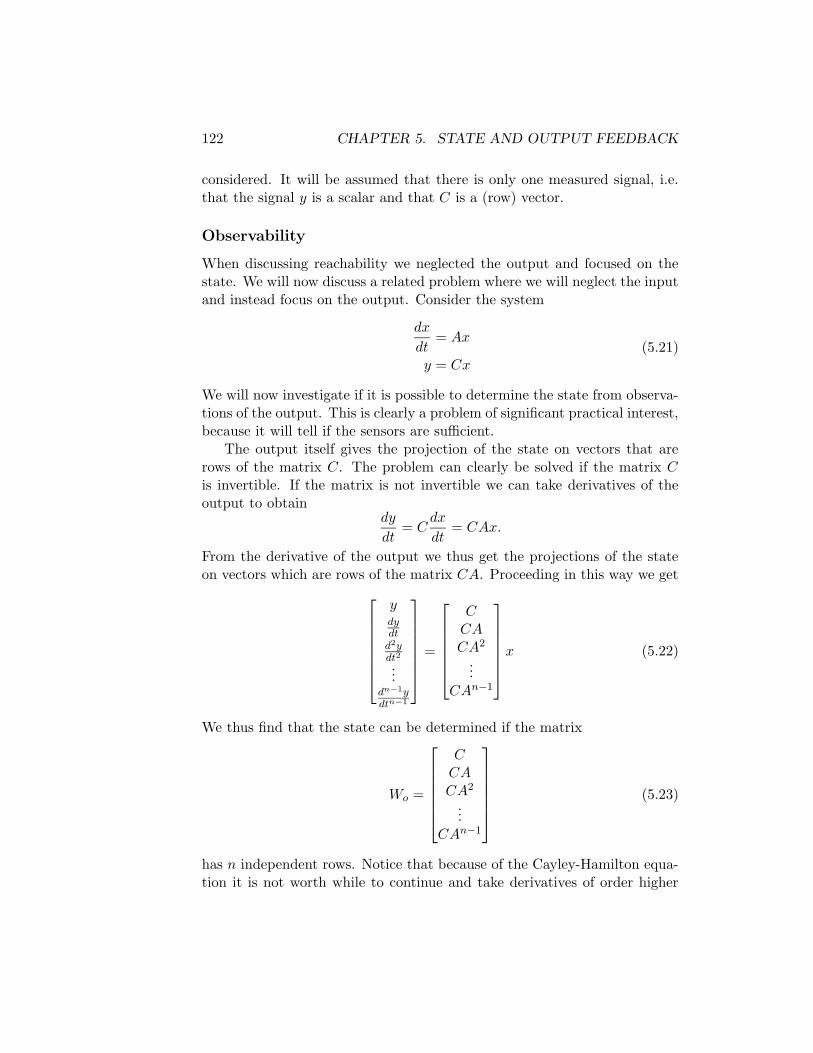
Figure 5.2: A non-observable system.

than n − 1. The matrix Wo is called the observability matrix. A systemis called observable if the observability matrix has full rank. We illustratewith an example.

Example 5.7 (Observability of the Inverted Pendulum). The linearized modelof inverted pendulum around the upright position is described by (5.4). Thematrices A and C are

A =

[

0 11 0

]

, C =[

1 0]

The observability matrix is

Wo =

[

1 00 1

]

which has full rank. It is thus possible to compute the state from a mea-surement of the angle.

The calculation can easily be extended to systems with inputs. The stateis then given by a linear combination of inputs and outputs and their higherderivatives. Differentiation can give very large errors when there is measure-ment noise and the method is therefore not very practical particularly whenderivatives of high order appear. A method that works with inputs will begiven the next section.

A Non-Observable System

It is useful to have an understanding of the mechanisms that make a systemunobservable. Such a system is shown in Figure 5.2. Next we will consider


the system in observable canonical form, i.e.

dz

dt=

−a1 1 0 . . . 0−a2 0 1 0

...−an−1 0 0 1−an 0 0 0

z +

b1b2...

bn−1

bn

u

y =[

1 0 0 . . . 0]

z +Du

A straight forward but tedious calculation shows that the inverse of theobservability matrix has a simple form. It is given by

W−1o =

1 0 0 . . . 0a1 1 0 . . . 0a2 a1 1 . . . 0...

an−1 an−2 an−3 . . . 1

This matrix is always invertible. The system is composed of two identi-cal systems whose outputs are added. It seems intuitively clear that it isnot possible to deduce the states from the output. This can also be seenformally.

Coordinate Changes

It is interesting to investigate how the observability matrix transforms whenthe coordinates are changed. Consider the system in equation (5.21). As-sume that the coordinates are changed to z = Tx. It follows from linearalgebra that the dynamics matrix and the output matrix are given by

A = TAT−1

C = CT−1.

The observability matrix for the transformed system then becomes

Wo =

C

CA

CA2

...

CAn−1

5.5. OBSERVERS 125

We have

CA = CT−1TAT−1 = CAT−1

CA2 = CT−1(TAT−1)2 = CT−1TAT−1TAT−1 = CA2T−1

...

CAn = CAnT−1

and we find that the observability matrix for the transformed system hasthe property

Wo =

C

CA

CA2

...

CAn−1

T−1 = WoT−1 (5.24)

This formula is very useful for finding the transformation matrix T .

5.5 Observers

For a system governed by equation (5.20), we can attempt to determinethe state simply by simulating the equations with the correct input. Anestimate of the state is then given by

dx

dt= Ax+Bu (5.25)

To find the properties of this estimate, introduce the estimation error

x = x− x

It follows from (5.20) and (5.25) that

dx

dt= Ax

If matrix A has all its eigenvalues in the left half plane, the error x willthus go to zero. Equation (5.25) is thus a dynamical system whose outputconverges to the state of the system (5.20).

The observer given by (5.25) uses only the process input u; the measuredsignal does not appear in the equation. It must also be required that thesystem is stable. We will therefore attempt to modify the observer so that


the output is used and that it will work for unstable systems. Consider thefollowing observer

dx

dt= Ax+Bu+ L(y − Cx). (5.26)

This can be considered as a generalization of (5.25). Feedback from themeasured output is provided by adding the term L(y − Cx). Notice thatCx = y is the output that is predicted by the observer. To investigate theobserver (5.26), form the error

x = x− x

It follows from (5.20) and (5.26) that

dx

dt= (A− LC)x

If the matrix L can be chosen in such a way that the matrix A − LC haseigenvalues with negative real parts, the error x will go to zero. The con-vergence rate is determined by an appropriate selection of the eigenvalues.

The problem of determining the matrix L such that A − LC has pre-scribed eigenvalues is very similar to the eigenvalue placement problem thatwas solved above. In fact, if we observe that the eigenvalues of the matrixand its transpose are the same, we find that could determine L such thatAT −CTLT has given eigenvalues. First we notice that the problem can besolved if the matrix

[

CT ATCT . . . A(n−1)TCT]

is invertible. Notice that this matrix is the transpose of the observabilitymatrix for the system (5.20).

Wo =

CCA...

CAn−1

of the system. Assume it is desired that the characteristic polynomial of thematrix A− LC is

p(s) = sn + p1sn−1 + . . .+ pn

It follows from Remark 5.1 of Theorem 5.1 that the solution is given by

LT =[

p1 − a1 p2 − a2 . . . pn − an

]

W To W

−To

5.5. OBSERVERS 127

where Wo is the observability matrix and Wo is the observability matrix ofthe system of the system

dz

dt=

−a1 1 0 . . . 0−a2 0 1 . . . 0

...−an−1 0 0 . . . 1−an 0 0 . . . 0

z +

b1b2...

bn−1

bn

u

y =[

1 0 0 . . . 0]

which is the observable canonical form of the system (5.20). Transposingthe formula for L we obtain

L = W−1o Wo

p1 − a1

p2 − a2...

pn − an

The result is summarized by the following theorem.

Theorem 5.2 (Observer design by eigenvalue placement). Consider the sys-tem given by

dx

dt= Ax+Bu

y = Cx

where output y is a scalar. Assume that the system is observable. Thedynamical system

dx

dt= Ax+Bu+ L(y − Cx)

with L chosen as

L = W−1o Wo

p1 − a1

p2 − a2...

pn − an

(5.27)

where the matrices Wo and Wo are given by

Wo =

CCA...

CAn−1

, W−1o =

1 0 0 . . . 0a1 1 0 . . . 0a2 a1 1 . . . 0...

an−1 an−2 an−3 . . . 1


PSfrag replacements

x˙xu −y

y

B Σ

Σ

∫

A

−C

−1

L

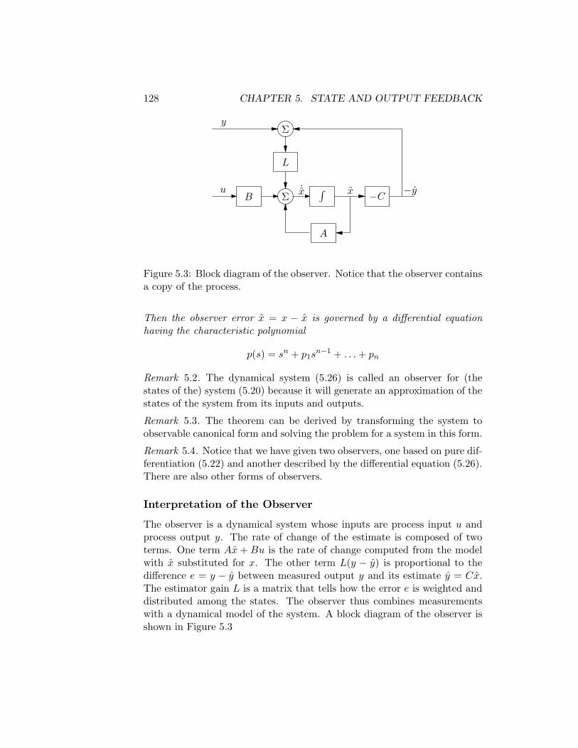
Figure 5.3: Block diagram of the observer. Notice that the observer containsa copy of the process.

Then the observer error x = x − x is governed by a differential equationhaving the characteristic polynomial

p(s) = sn + p1sn−1 + . . .+ pn

Remark 5.2. The dynamical system (5.26) is called an observer for (thestates of the) system (5.20) because it will generate an approximation of thestates of the system from its inputs and outputs.

Remark 5.3. The theorem can be derived by transforming the system toobservable canonical form and solving the problem for a system in this form.

Remark 5.4. Notice that we have given two observers, one based on pure dif-ferentiation (5.22) and another described by the differential equation (5.26).There are also other forms of observers.

Interpretation of the Observer

The observer is a dynamical system whose inputs are process input u andprocess output y. The rate of change of the estimate is composed of twoterms. One term Ax + Bu is the rate of change computed from the modelwith x substituted for x. The other term L(y − y) is proportional to thedifference e = y − y between measured output y and its estimate y = Cx.The estimator gain L is a matrix that tells how the error e is weighted anddistributed among the states. The observer thus combines measurementswith a dynamical model of the system. A block diagram of the observer isshown in Figure 5.3

5.5. OBSERVERS 129

Duality

Notice the similarity between the problems of finding a state feedback andfinding the observer. The key is that both of these problems are equivalentto the same algebraic problem. In eigenvalue placement it is attempted tofind L so that A − BL has given eigenvalues. For the observer design itis instead attempted to find L so that A − LC has given eigenvalues. Thefollowing equivalence can be established between the problems

A↔ AT

B ↔ CT

K ↔ LT

Wr ↔W To

The similarity between design of state feedback and observers also meansthat the same computer code can be used for both problems.

Computing the Observer Gain

The observer gain can be computed in several different ways. For simpleproblems it is convenient to introduce the elements of L as unknown param-eters, determine the characteristic polynomial of the observer det (A− LC)and identify it with the desired characteristic polynomial. Another alterna-tive is to use the fact that the observer gain can be obtained by inspectionif the system is in observable canonical form. In the general case the ob-server gain is then obtained by transformation to the canonical form. Thereare also reliable numerical algorithms. They are identical to the algorithmsfor computing the state feedback. The procedures are illustrated by a fewexamples.

Example 5.8 (The Double Integrator). The double integrator is described by

dx

dt=

[

0 10 0

]

x+

[

01

]

u

y =[

1 0]

The observability matrix is

Wo =

[

1 00 1

]


i.e. the identity matrix. The system is thus observable and the problem canbe solved. We have

A− LC =

[

−l1 1−l2 0

]

It has the characteristic polynomial

detA− LC = det

[

s+ l1 −1−l2 s

]

= s2 + l1s+ l2

Assume that it is desired to have an observer with the characteristic poly-nomial

s2 + p1s+ p2 = s2 + 2ζωs+ ω2

The observer gains should be chosen as

l1 = p1 = 2ζω

l2 = p2 = ω2

The observer is then

dx

dt=

[

0 10 0

]

x+

[

01

]

u+

[

l1l2

]

(y − x1)

5.6 Output FeedbackÄ

In this section we will consider the same system as in the previous sections,i.e. the nth order system described by

dx

dt= Ax+Bu

y = Cx(5.28)

where only the output is measured. As before it will be assumed that u andy are scalars. It is also assumed that the system is reachable and observable.In Section 5.3 we had found a feedback

u = −Kx+Krr

for the case that all states could be measured and in Section 5.4 we havepresented developed an observer that can generate estimates of the state xbased on inputs and outputs. In this section we will combine the ideas ofthese sections to find an feedback which gives desired closed loop eigenvaluesfor systems where only outputs are available for feedback.

5.6. OUTPUT FEEDBACK 131

If all states are not measurable, it seems reasonable to try the feedback

u = −Kx+Krr (5.29)

where x is the output of an observer of the state (5.26), i.e.

dx

dt= Ax+Bu+ L(y − Cx) (5.30)

Since the system (5.28) and the observer (5.30) both are of order n, theclosed loop system is thus of order 2n. The states of the system are x andx. The evolution of the states is described by equations (5.28), (5.29)(5.30).To analyze the closed loop system, the state variable x is replace by

x = x− x (5.31)

Subtraction of (5.28) from (5.28) gives

dx

dt= Ax−Ax− L(y − Cx) = Ax− LCx = (A− LC)x

Introducing u from (5.29) into this equation and using (5.31) to eliminate xgives

dx

dt= Ax+Bu = Ax−BKx+BKrr = Ax−BK(x− x) +BKrr

= (A−BK)x+BKx+BKrr

The closed loop system is thus governed by

d

dt

[

xx

]

=

[

A−BK BK0 A− LC

] [

xx

]

+

[

BKr

0

]

r (5.32)

Since the matrix on the right-hand side is block diagonal, we find that thecharacteristic polynomial of the closed loop system is

det (sI −A+BK) det (sI −A+ LC)

This polynomial is a product of two terms, where the first is the charac-teristic polynomial of the closed loop system obtained with state feedbackand the other is the characteristic polynomial of the observer error. Thefeedback (5.29) that was motivated heuristically thus provides a very neatsolution to the eigenvalue placement problem. The result is summarized asfollows.


Theorem 5.3 (Pole placement by output feedback). Consider the system

dx

dt= Ax+Bu

y = Cx

The controller described by

u = −Kx+Krr

dx

dt= Ax+Bu+ L(y − Cx)

gives a closed loop system with the characteristic polynomial

det (sI −A+BK) det (sI −A+ LC)

This polynomial can be assigned arbitrary roots if the system is observableand reachable.

Remark 5.5. Notice that the characteristic polynomial is of order 2n andthat it can naturally be separated into two factors, one det (sI −A+BK)associated with the state feedback and the other det (sI −A+ LC) with theobserver.

Remark 5.6. The controller has a strong intuitive appeal. It can be thoughtof as composed of two parts, one state feedback and one observer. Thefeedback gain K can be computed as if all state variables can be measured.

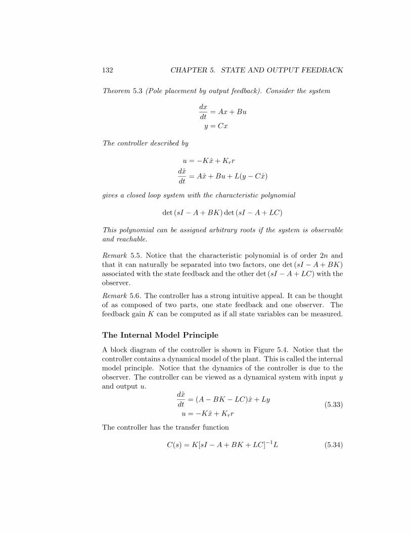
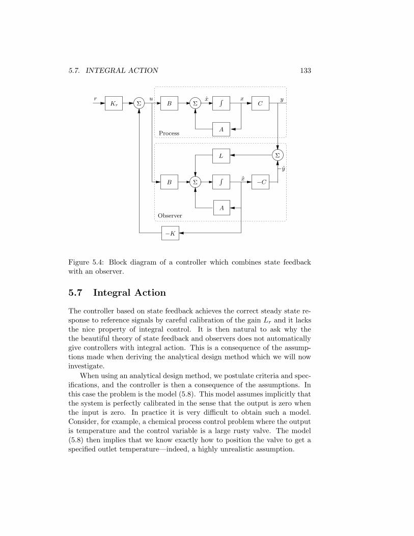
The Internal Model Principle

A block diagram of the controller is shown in Figure 5.4. Notice that thecontroller contains a dynamical model of the plant. This is called the internalmodel principle. Notice that the dynamics of the controller is due to theobserver. The controller can be viewed as a dynamical system with input yand output u.

dx

dt= (A−BK − LC)x+ Ly

u = −Kx+Krr(5.33)

The controller has the transfer function

C(s) = K[sI −A+BK + LC]−1L (5.34)

5.7. INTEGRAL ACTION 133

PSfrag replacementsr u yxx

x

−y

B

B

Σ

Σ

Σ

Σ

R

R

A

A

C

−C

L

−K

Kr

Process

Observer

Figure 5.4: Block diagram of a controller which combines state feedbackwith an observer.

5.7 Integral Action

The controller based on state feedback achieves the correct steady state re-sponse to reference signals by careful calibration of the gain Lr and it lacksthe nice property of integral control. It is then natural to ask why thethe beautiful theory of state feedback and observers does not automaticallygive controllers with integral action. This is a consequence of the assump-tions made when deriving the analytical design method which we will nowinvestigate.

When using an analytical design method, we postulate criteria and spec-ifications, and the controller is then a consequence of the assumptions. Inthis case the problem is the model (5.8). This model assumes implicitly thatthe system is perfectly calibrated in the sense that the output is zero whenthe input is zero. In practice it is very difficult to obtain such a model.Consider, for example, a chemical process control problem where the outputis temperature and the control variable is a large rusty valve. The model(5.8) then implies that we know exactly how to position the valve to get aspecified outlet temperature—indeed, a highly unrealistic assumption.


Having understood the difficulty it is not too hard to change the model.By modifying the model to

dx

dt= Ax+B(u+ v)

y = Cx,(5.35)

where v is an unknown constant, we can can capture the idea that the modelis no longer perfectly calibrated. This model is called a model with an inputdisturbance. Another possibility is to use the model

dx

dt= Ax+Bu

y = Cx+ v

where v is an unknown constant. This is a model with an output disturbance.It will now be shown that a straightforward design of an output feedback forthis system does indeed give integral action. Both disturbance models willproduce controllers with integral action. We will start by investigating thecase of an input disturbance. This is a little more convenient for us becauseit fits the control goal of finding a controller that drives the state to zero.

The model with an input disturbance can conveniently be brought intothe framework of state feedback. To do this, we first observe that v is anunknown constant which can be described by

dv

dt= 0

To bring the system into the standard format we simply introduce the dis-turbance v as an extra state variable. The state of the system is thus

z =

[

xv

]

This is also called state augmentation. Using the augmented state the model(5.35) can be written as

d

dt

[

xv

]

=

[

A B0 0

] [

xv

]

+

[

B0

]

u

y =[

C 0]

[

xv

] (5.36)

Notice that the disturbance state is not reachable. If the disturbance canbe measured, the state feedback is then

u = −Kz +Krr = −Kxx−Kvv +Krr (5.37)

5.8. A GENERAL CONTROLLER STRUCTURE 135

The disturbance state v is not reachable. The the effect of the disturbanceon the system can, however, be eliminated by choosing Kv = 1. If the distur-bance v is known the control law above can be interpreted as a combinationof feedback from the system state and feedforward from a measured distur-bance. It is not realistic to assume that the disturbance can be measuredand we will instead replace the states by estimates. The feedback law thenbecomes

u = −Kxz +Krr = −Kxx− v +Krr

This means that feedback is based on estimates of the state and the distur-bance. There are many other ways to introduce integral action.

5.8 A General Controller Structure

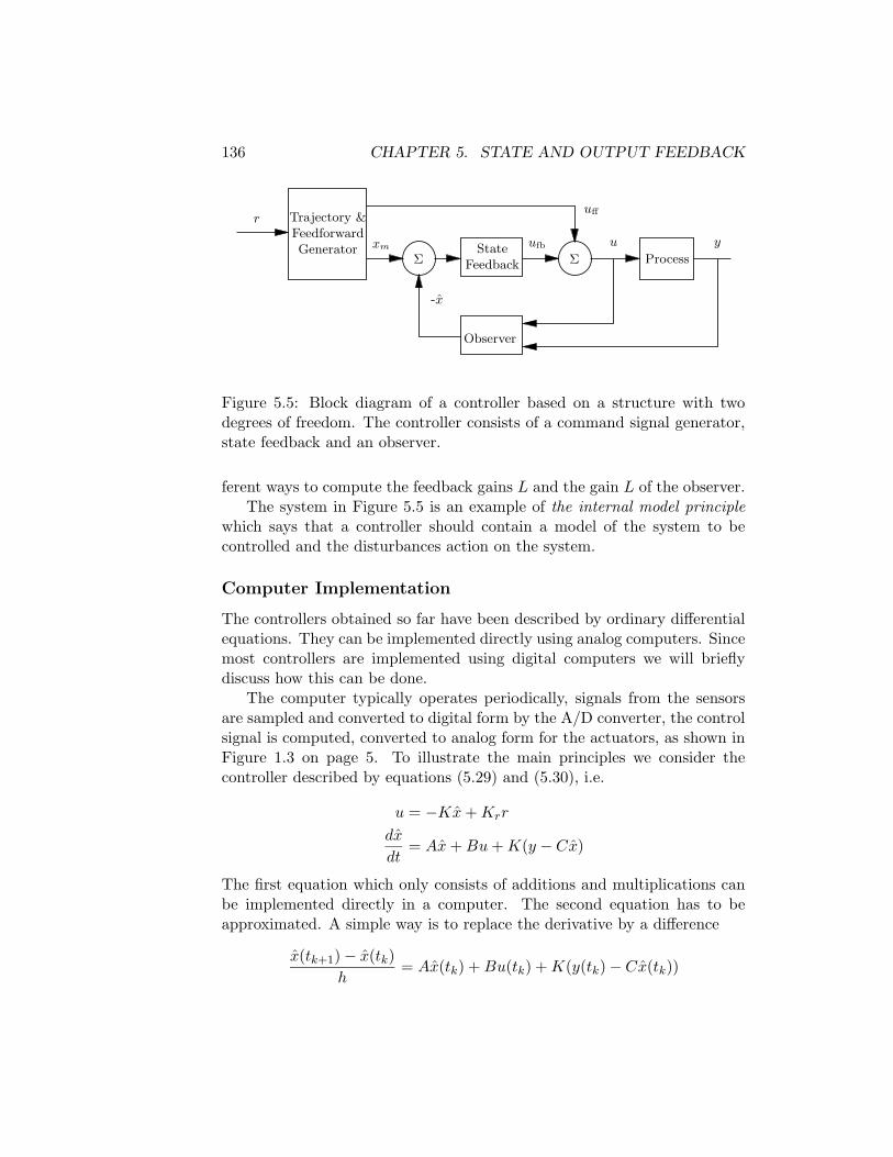
So far reference signals have been introduced simply by adding it to the statefeedback. A more sophisticated way of doing this is shown by the block dia-gram in Figure 5.5, where the controller consists of three parts: an observerthat computes estimates of the states based on a model and measured pro-cess inputs and outputs, a state feedback and a trajectory generator thatgenerates the desired behavior of all states xm and a feedforward signal uff.The signal uff is such that it generates the desired behavior of the stateswhen applied to the system, under ideal conditions of no disturbances andno modeling errors. The controller is said to have two degrees of freedombecause the response to command signals and disturbances are decoupled.Disturbance responses are governed by the observer and the state feedbackand the response to command signal is governed by the feedforward. To getsome insight into the behavior of the system let us discuss what happenswhen the command signal is changed. To fix the ideas let us assume thatthe system is in equilibrium with the observer state x equal to the processstate x. When the command signal is changed a feedforward signal uff(t) isgenerated. This signal has the property that the process output gives thedesired output xm(t) when the feedforward signal is applied to the system.The process state changes in response to the feedforward signal. The ob-server tracks the state perfectly because the initial state was correct. Theestimated state x will be equal to the desired state xm and the feedbacksignal L(xm − x) is zero. If there are some disturbances or some modelingerrors the feedback signal will be different from zero and attempt to correctthe situation.

The controller given in Figure 5.5 is a very general structure. There aremany ways to generate the feedforward signal and there are also many dif-


PSfrag replacements

Trajectory &FeedforwardGenerator

r

u

-x

y

xm

ProcessΣ ΣState

Feedback

Observer

ufb

uff

y

Figure 5.5: Block diagram of a controller based on a structure with twodegrees of freedom. The controller consists of a command signal generator,state feedback and an observer.

ferent ways to compute the feedback gains L and the gain L of the observer.The system in Figure 5.5 is an example of the internal model principle

which says that a controller should contain a model of the system to becontrolled and the disturbances action on the system.

Computer Implementation

The controllers obtained so far have been described by ordinary differentialequations. They can be implemented directly using analog computers. Sincemost controllers are implemented using digital computers we will brieflydiscuss how this can be done.

The computer typically operates periodically, signals from the sensorsare sampled and converted to digital form by the A/D converter, the controlsignal is computed, converted to analog form for the actuators, as shown inFigure 1.3 on page 5. To illustrate the main principles we consider thecontroller described by equations (5.29) and (5.30), i.e.

u = −Kx+Krr

dx

dt= Ax+Bu+K(y − Cx)

The first equation which only consists of additions and multiplications canbe implemented directly in a computer. The second equation has to beapproximated. A simple way is to replace the derivative by a difference

x(tk+1) − x(tk)

h= Ax(tk) +Bu(tk) +K(y(tk) − Cx(tk))

5.9. EXERCISES 137

where tk are the sampling instants and h = tk+1− tk is the sampling period.Rewriting the equation we get

x(tk+1 = x(tk) + h(

Ax(tk) +Bu(tk) +K(y(tk) − Cx(tk)))

. (5.38)

The calculation of the state only requires addition and multiplication andcan easily be done by a computer. A pseudo code for the program that runsin the digital computer is

"Control algorithm - main loop

r=adin(ch1) "read setpoint from ch1

y=adin(ch2) "read process variable from ch2

u=C*x+Kr*r "compute control variable

daout(ch1) "set analog output ch1

x=x+h*(A*x+B*u+L*(y-C*x)) "update state estimate

The program runs periodically. Notice that the number of computationsbetween reading the analog input and setting th analog output has beenminimized. The state is updated after the analog output has been set. Theprogram has one states x. The choice of sampling period requires some care.

For linear systems the difference approximation can be avoided by ob-serving that the control signal is constant over the sampling period. Anexact theory for this can be developed. Doing this we get a control law thatis identical to (5.38) but with slightly different coefficients.

There are several practical issues that also must be dealt with. For ex-ample it is necessary to filter a signal before it is sampled so that the filteredsignal has little frequency content above fs/2 where fs is the sampling fre-quency. If controllers with integral action are used it is necessary to provideprotection so that the integral does not become too large when the actuatorsaturates. Care must also be taken so that parameter changes do not causedisturbances. Some of these issues are discussed in Chapter 10.

5.9 Exercises

1. Consider a system on reachable canonical form. Show that the inverse ofthe reachability matrix is given by

W−1r =

1 a1 a2 . . . an

0 1 a1 . . . an−1...0 0 0 . . . 1

(5.39)


Documents

State and Output Feedback