Stat. 758: Computation andProgramming

Eric B. Laber

Department of Statistics, North Carolina State University

Lecture 3Sept. 3, 2015

Luck is not as random as you think. Beforethat lottery ticket won the jackpot, someonehad to buy it.—Calendar of Perpetual Inspiration

We are all stupider for having read theabove quote.—Eric B. Laber

House keeping

I No class on Thursday Sept 3

I HW 1 is posted (prepare for non-null time investment)

I Python is on the lab machines in SAS hall

I Work together! But turn in our your own HW and write yourown code!

Warm-up

I Explain to your stat buddyI What is a random number?I How can you test whether a sample, say X1, . . . ,Xn, is

generated from a pre-specified distribution?

I Suppose you could generate a random sequence of ind.Bernoulli random variables how could you use these toconstruct a draw from a Uniform[0, 1] distribution?

I True or false:

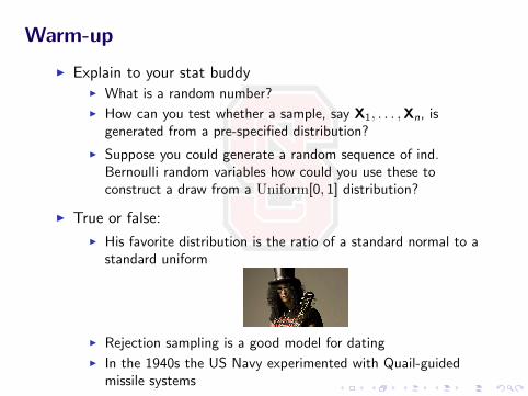
I His favorite distribution is the ratio of a standard normal to astandard uniform

I Rejection sampling is a good model for datingI In the 1940s the US Navy experimented with Quail-guided

missile systems

The road so far

I Python basics

I Syntax and basic data types

I Control-flow

I Functions, scope, and modules

I Planning for numerical computing

I Identifying challenges and choices

I Alternative programming design patterns, e.g., loops vs.recursion

Today: random number generation

I Stochasticity essential in almost all statistical simulation

I Std MC study: random generate training data from model,apply method, evaluate using random test data, and repeat

I Std model evaluation: randomly generate data from postulatedmodel, compare with observed data, repeat

I (Almost) any programming language has built-in libraries forrandom number generation

I E.g., we used numpy.random.exponential in our queue sim

I Why should we worry about random number generation?

Random number generation basics

I A computer (in isolation) cannot generate random numbers

I Deterministic operations

I Idea! Generate deterministic sequences of pseudo randomsequences that ‘appear’ to be random

I Canonical example: linear congruential generator (lcg)

Set X0 to starting value in Z+, then recursively

Xn+1 = (aXn + c) mod m,

where a, c ,m ∈ Z+ are fixed non-negative integers

I In class: prove this has period at most m

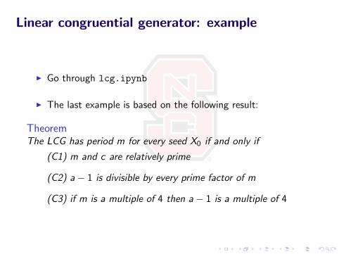
Linear congruential generator: example

I Go through lcg.ipynb

I The last example is based on the following result:

TheoremThe LCG has period m for every seed X0 if and only if

(C1) m and c are relatively prime

(C2) a− 1 is divisible by every prime factor of m

(C3) if m is a multiple of 4 then a− 1 is a multiple of 4

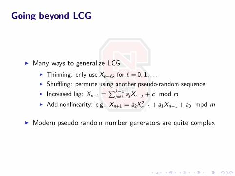
Going beyond LCG

I Many ways to generalize LCG

I Thinning: only use Xs+`k for ` = 0, 1, . . .

I Shuffling: permute using another pseudo-random sequence

I Increased lag: Xn+1 =∑k−1

j=0 ajXn−j + c mod m

I Add nonlinearity: e.g., Xn+1 = a2X2n−1 + a1Xn−1 + a0 mod m

I Modern pseudo random number generators are quite complex

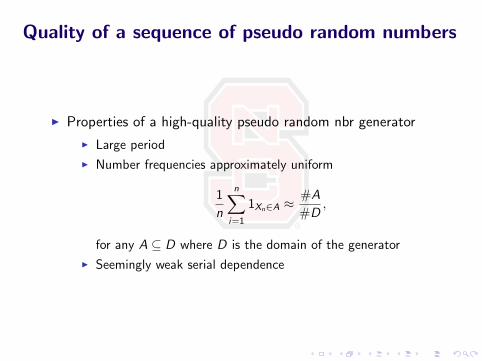
Quality of a sequence of pseudo random numbers

I Properties of a high-quality pseudo random nbr generator

I Large period

I Number frequencies approximately uniform

1

n

n∑i=1

1Xn∈A ≈#A

#D,

for any A ⊆ D where D is the domain of the generator

I Seemingly weak serial dependence

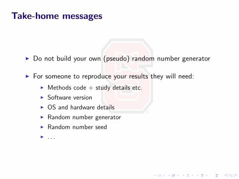
Take-home messages

I Do not build your own (pseudo) random number generator

I For someone to reproduce your results they will need:

I Methods code + study details etc.

I Software version

I OS and hardware details

I Random number generator

I Random number seed

I . . .

Generating random variables

I Hereafter we assume access to iid draws from Uniform[0, 1]

I Goal: build more complex random objects

I Univariate random variables

I Multivariate random variables

I Continuous-time stochastic processes

I More general stochastic processes

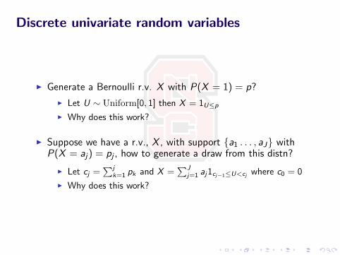
Discrete univariate random variables

I Generate a Bernoulli r.v. X with P(X = 1) = p?

I Let U ∼ Uniform[0, 1] then X = 1U≤p

I Why does this work?

I Suppose we have a r.v., X , with support {a1 . . . , aJ} withP(X = aj) = pj , how to generate a draw from this distn?

I Let cj =∑j

k=1 pk and X =∑J

j=1 aj1cj−1≤U<cj where c0 = 0

I Why does this work?

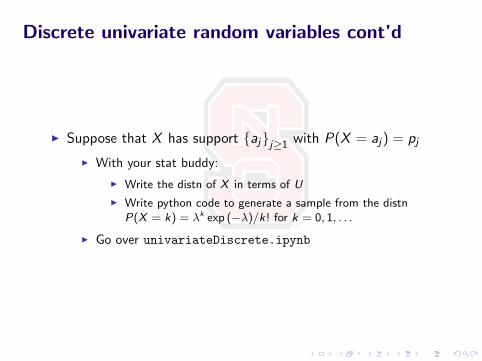
Discrete univariate random variables cont’d

I Suppose that X has support {aj}j≥1 with P(X = aj) = pj

I With your stat buddy:

I Write the distn of X in terms of U

I Write python code to generate a sample from the distnP(X = k) = λk exp (−λ)/k! for k = 0, 1, . . .

I Go over univariateDiscrete.ipynb

Discrete univariate random variables cont’d

I Discussed simple methods for sampling from d.u.r.v.’s

I Built-in random sampling functions in numpy.random seehttp://docs.scipy.org/doc/numpy/reference/

routines.random.html

I Built-in functions highly optimized for speed, a good referencefor these funtions is “Random number generation” by Gentle

I Many statistical approximations to continuous distributions arediscrete, e.g., empirical distn, copulas, etc.

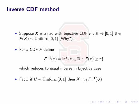
Inverse CDF method

I Suppose X is a r.v. with bijective CDF F : R→ [0, 1] thenF (X ) ∼ Uniform[0, 1] (Why?)

I For a CDF F define

F−1(τ) = inf {x ∈ R : F (x) ≥ τ}

which reduces to usual inverse in bijective case

I Fact: if U ∼ Uniform[0, 1] then X =D F−1(U)

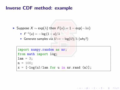
Inverse CDF method: example

I Suppose X ∼ exp(λ) then F (x) = 1− exp(−λx)

I F−1(u) = − log (1− u)/λ

I Generate samples via U 7→ − log(U)/λ (why?)

import numpy.random as nr;

from math import log;

lam = 3;

n = 100;

x = [-log(u)/lam for u in nr.rand (n)];

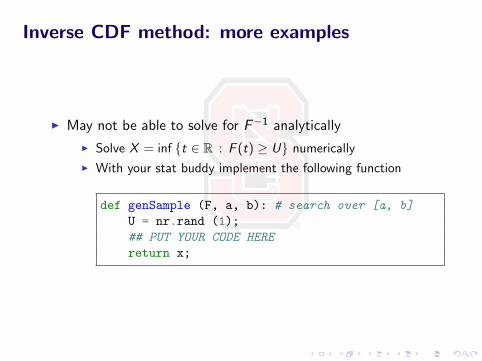
Inverse CDF method: more examples

I May not be able to solve for F−1 analytically

I Solve X = inf {t ∈ R : F (t) ≥ U} numerically

I With your stat buddy implement the following function

def genSample (F, a, b): # search over [a, b]

U = nr.rand (1);

## PUT YOUR CODE HERE

return x;

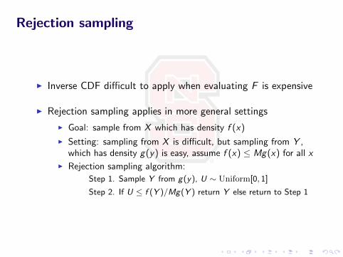
Rejection sampling

I Inverse CDF difficult to apply when evaluating F is expensive

I Rejection sampling applies in more general settings

I Goal: sample from X which has density f (x)

I Setting: sampling from X is difficult, but sampling from Y ,which has density g(y) is easy, assume f (x) ≤ Mg(x) for all x

I Rejection sampling algorithm:

Step 1. Sample Y from g(y), U ∼ Uniform[0, 1]

Step 2. If U ≤ f (Y )/Mg(Y ) return Y else return to Step 1

Rejection sampling cont’d

I Rejection sampling will perform best if f andg are close

I If g is a poor surrogate for f then rejection sampling can behighly inefficient

I Go over rejection.ipynb

Rejection sampling wrap-up

I Rejection sampling widely used

I Many variants including automatically adaptive majorization

I Basis for Metropolis sampling

I Closely related to ‘hit-or-miss’ algorithms for evaluatingintegrals (we’ll talk about these later)

I A related idea is the ratio-of-uniforms methods which you willinvestigate in homework 1

Break: Warm-up quiz II

I Explain to you stat buddy

I What is the CONAN principle for normal random vectors?

I What is the eigen decomposition of a pd matrix?

I What is a Gaussian process?

I True or false:

I A (provably) prime number with 39 digits was discoveredbefore Penicillin

I A sigma algebra is either finite or uncountably infinite

I At Bob’s bear bait (.com) you can buy a 55 gallon drum oftrailmix for 68 dollars

Multivariate normal distribution

I If Z ∼ Np(0, I ) then

b + AZ ∼ Np(b,AᵀA),

where b ∈ Rp and A ∈ Rp×p

I How can we use this generate a draw from Np(µ,Σ) distn?

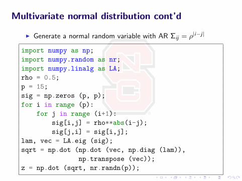
Multivariate normal distribution cont’d

I Generate a normal random variable with AR Σij = ρ|i−j |

import numpy as np;

import numpy.random as nr;

import numpy.linalg as LA;

rho = 0.5;

p = 15;

sig = np.zeros (p, p);

for i in range (p):

for j in range (i+1):

sig[i,j] = rho**abs(i-j);

sig[j,i] = sig[i,j];

lam, vec = LA.eig (sig);

sqrt = np.dot (np.dot (vec, np.diag (lam)),

np.transpose (vec));

z = np.dot (sqrt, nr.randn(p));

Numerical linear algebra (and such)

I Preceding example illustrates that we’ll need more numericaltools from python

I Next time we’ll explore the numpy and scipy libraries

I Then back to simulation for bit