Embed Size (px)
Citation preview
STAT 545AClass meeting #9Wednesday, October 3, 2012
Dr. Jennifer (Jenny) Bryan
Department of Statistics and Michael Smith Laboratories
Review of last class
lattice graphics: to get good results, you only need to learn basic commands and arguments
To get great results, you need to be courageous and specify lots of seemingly arcane arguments, redefine lists of graphics parameters, and redefine panel functions. BUT it’s not as hard as it seems! Walk before you run. But get moving.
Typical workflow: “so so” plot using built-in facilities. Gradually take control of what you need to change by first doing nothing (i.e. specifying the graphics parameters or the panel function but specify the default!), then baby step up to the full glorious figure you want.
Review of last class
Another fruitful approach: find a plot in Sarkar’s or Murrell’s book (or in this class), go get the code that produced it and slowly “substitute” your data and desires into the original
the “type” argument is extremely useful!
show.settings() and trellis.par.get() are useful for grasping what default colors, symbols, etc. are, so you can take control and substitute your own colors, symbols, etc.
high-volume scatterplots benefit from some fancier treatment: hexagonal binning, 2-dimensional density estimation
For next Wednesday:I’d like you to start your page for the final project. At the very least, give a brief description of what you plan to do. Link to a data source. Pose some questions you might try to answer or some issues you hope to explore.
Ideally you will be making even more progress, i.e. working on data acquisition, import, cleaning.
Now I will continue my efforts to turn you all into professional R scripters ........
“Habits of highly effective programmers”

“Source is real.”
Philosophy practiced by the pros
“The source code is real. The objects are realizations of the source code. Source for EVERY user modified object is placed in a particular directory or directories, for later editing and retrieval.”
-- from the ESS manual
Jenny’s slight expansion ...Actually, there are a few other things that are real, besides source code.
Input data: perfectly preserved file of data as it came from it’s “producer” (maybe revoke write permission?)
Clean data: plain text, delimited, clean data file that you created from the mess you got above (maybe revoke write permission?)
Figures: lots of them, with meaningful names, stored to file(s) using a command (not the mouse)
Important statistical results: stored to file with a command in the plainest form possible, i.e. plain text if feasible or as R objects otherwise
The other philosophy
R objects are real. Figures you see popping up on your screen are real. The R code you typed at the command line late last night is real.
R objects are created by typing at the command line and are changed using fix() or are recreated. R workspaces are saved and reloaded. Etc.
I cannot responsibly recommend this approach.
If you’re in this class, you’re the kind of person for whom this approach is not robust.
Why “source code is real”?• “Objects are real” comes more naturally to those
accustomed to a GUI, to Excel, etc.
• “Source is real” places emphasis on the logic of your analysis, not on the specific numerical result obtained by applying it to a dataset.
• “Source is real” leaves us in a much better position to replicate the analysis -- perhaps with the same data, perhaps not -- or to use it as the starting point for a new analysis.
• “Source is real” approach has a built-in mechanism for documenting exactly what was done.
• Jenny’s modification to the philosphy acknowledges that we don’t always want to go back and rerun everything.
“Source code is real”: how to implement
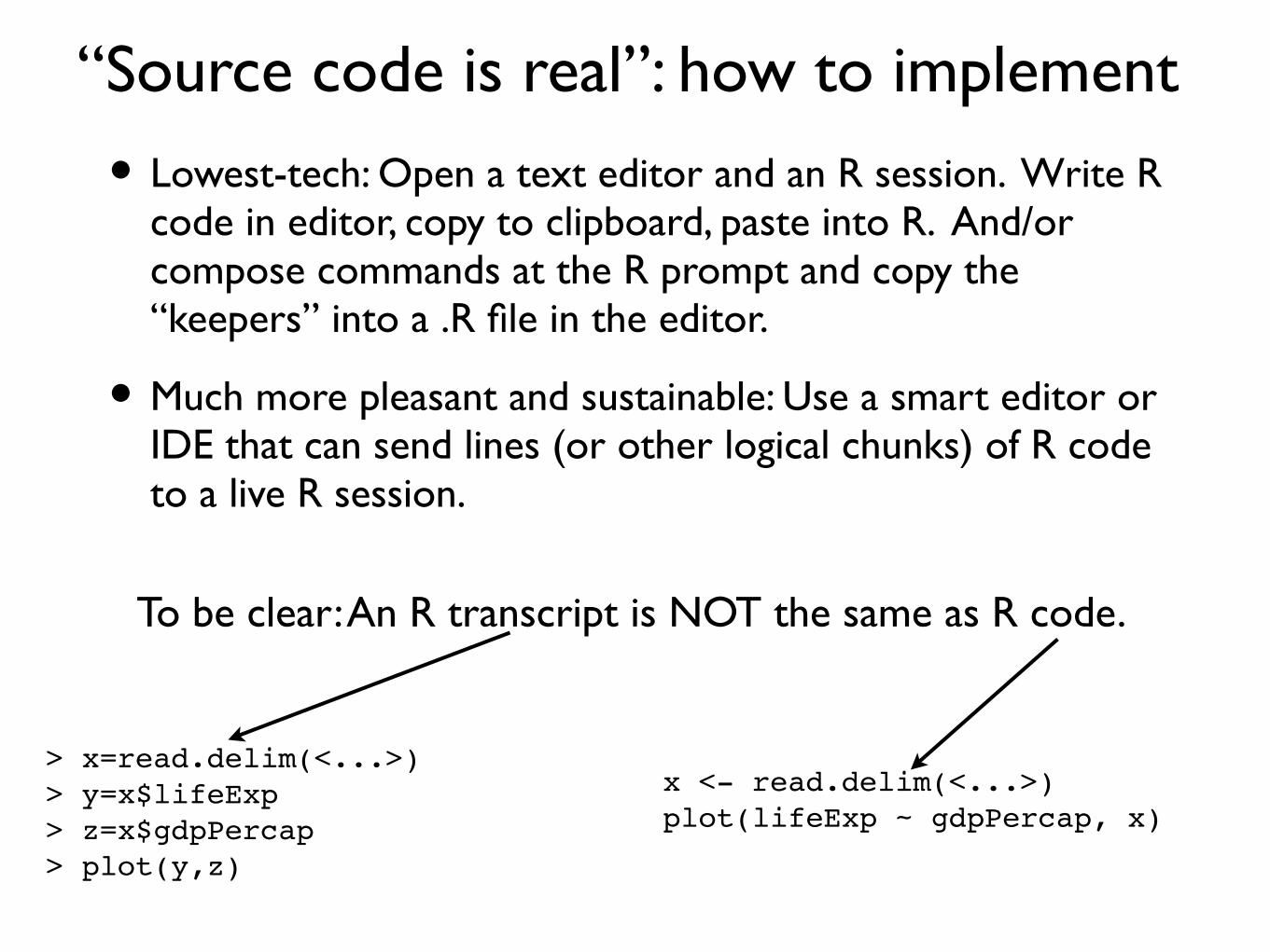
• Lowest-tech: Open a text editor and an R session. Write R code in editor, copy to clipboard, paste into R. And/or compose commands at the R prompt and copy the “keepers” into a .R file in the editor.
• Much more pleasant and sustainable: Use a smart editor or IDE that can send lines (or other logical chunks) of R code to a live R session.
To be clear: An R transcript is NOT the same as R code.
> x=read.delim(<...>)> y=x$lifeExp> z=x$gdpPercap> plot(y,z)
x <- read.delim(<...>)plot(lifeExp ~ gdpPercap, x)
coding style & standards

Let us change our traditional attitude to the construction of programs. Instead of imagining that our main task is to instruct a computer what to do, let us concentrate rather on explaining to human beings what we want a computer to do. - Donald E. Knuth
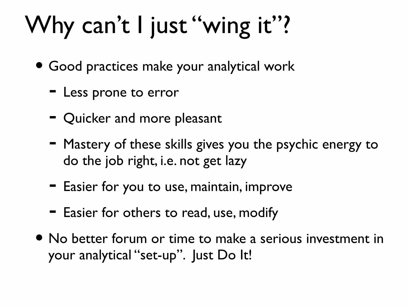
Why can’t I just “wing it”?
• Good practices make your analytical work
- Less prone to error
- Quicker and more pleasant
- Mastery of these skills gives you the psychic energy to do the job right, i.e. not get lazy
- Easier for you to use, maintain, improve
- Easier for others to read, use, modify
• No better forum or time to make a serious investment in your analytical “set-up”. Just Do It!
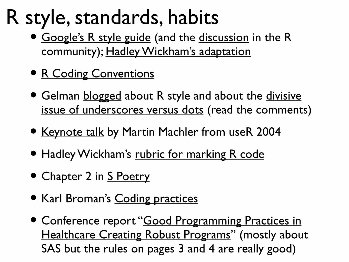
R style, standards, habits• Google’s R style guide (and the discussion in the R
community); Hadley Wickham’s adaptation
• R Coding Conventions
• Gelman blogged about R style and about the divisive issue of underscores versus dots (read the comments)
• Keynote talk by Martin Machler from useR 2004
• Hadley Wickham’s rubric for marking R code
• Chapter 2 in S Poetry
• Karl Broman’s Coding practices
• Conference report “Good Programming Practices in Healthcare Creating Robust Programs” (mostly about SAS but the rules on pages 3 and 4 are really good)
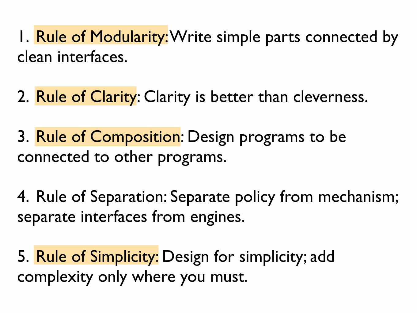
1. Rule of Modularity: Write simple parts connected by clean interfaces.
2. Rule of Clarity: Clarity is better than cleverness.
3. Rule of Composition: Design programs to be connected to other programs.
4. Rule of Separation: Separate policy from mechanism; separate interfaces from engines.
5. Rule of Simplicity: Design for simplicity; add complexity only where you must.
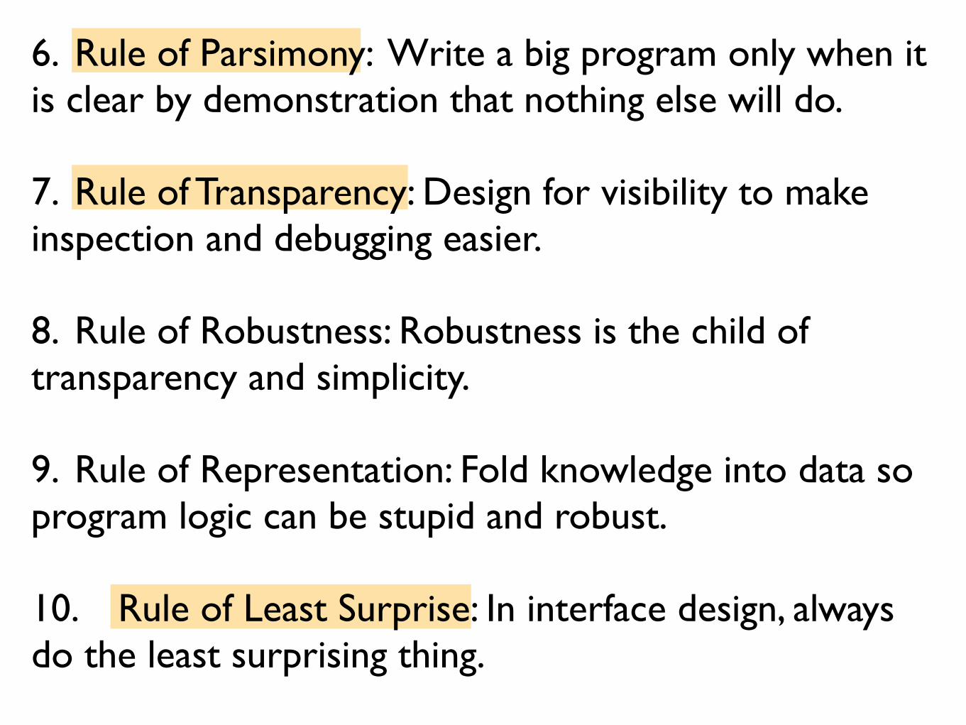
6. Rule of Parsimony: Write a big program only when it is clear by demonstration that nothing else will do.
7. Rule of Transparency: Design for visibility to make inspection and debugging easier.
8. Rule of Robustness: Robustness is the child of transparency and simplicity.
9. Rule of Representation: Fold knowledge into data so program logic can be stupid and robust.
10. Rule of Least Surprise: In interface design, always do the least surprising thing.
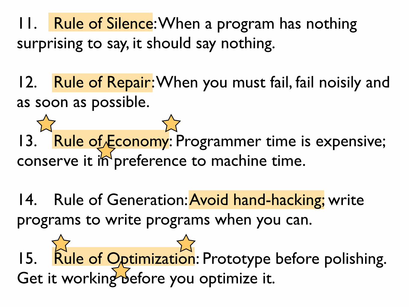
11. Rule of Silence: When a program has nothing surprising to say, it should say nothing.
12. Rule of Repair: When you must fail, fail noisily and as soon as possible.
13. Rule of Economy: Programmer time is expensive; conserve it in preference to machine time.
14. Rule of Generation: Avoid hand-hacking; write programs to write programs when you can.
15. Rule of Optimization: Prototype before polishing. Get it working before you optimize it.

16. Rule of Diversity: Distrust all claims for “one true way”.
17. Rule of Extensibility: Design for the future, because it will be here sooner than you think.
Coding conventions
• Trust me -- certain practices will make your coding life much more pleasant
• Use indenting
• Use spaces around binary operators and after commas
• Wrap your lines
• Use comments (and indent properly)
• Develop naming conventions for yourself
• Lots of this is automatic or very very easy with the right editor/IDE setup, e.g. Emacs Speaks Statistics or Rstudio ... they didn’t build this stuff in for jollies, people! It’s useful.
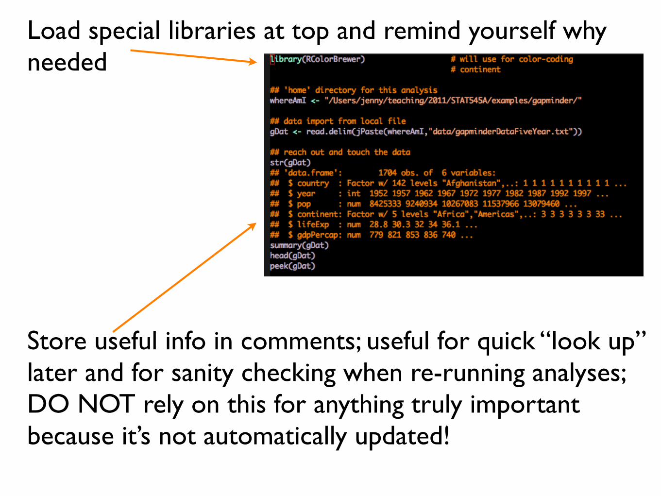
Load special libraries at top and remind yourself why needed
Store useful info in comments; useful for quick “look up” later and for sanity checking when re-running analyses; DO NOT rely on this for anything truly important because it’s not automatically updated!
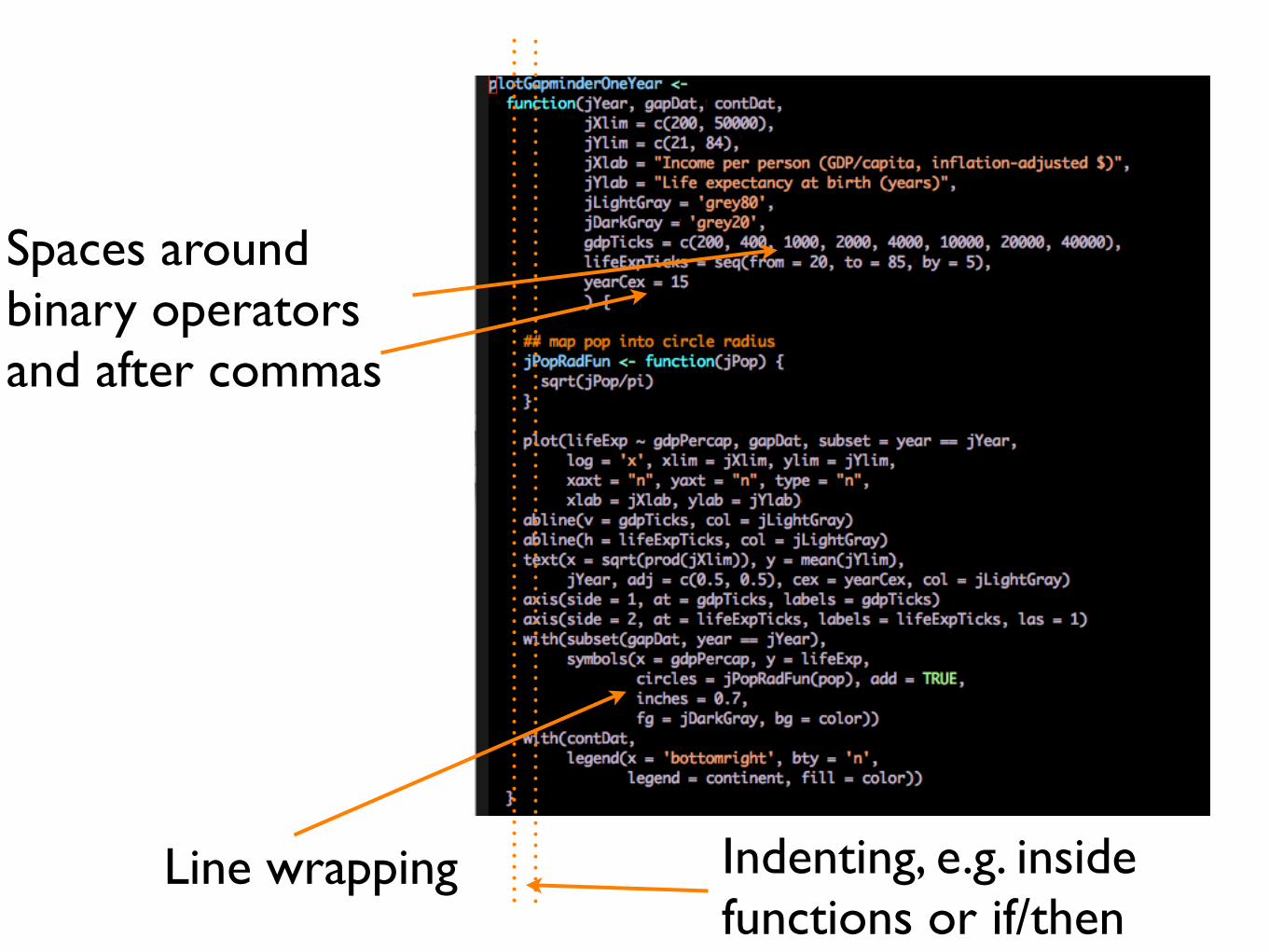
Line wrapping Indenting, e.g. inside functions or if/then
Spaces around binary operators and after commas
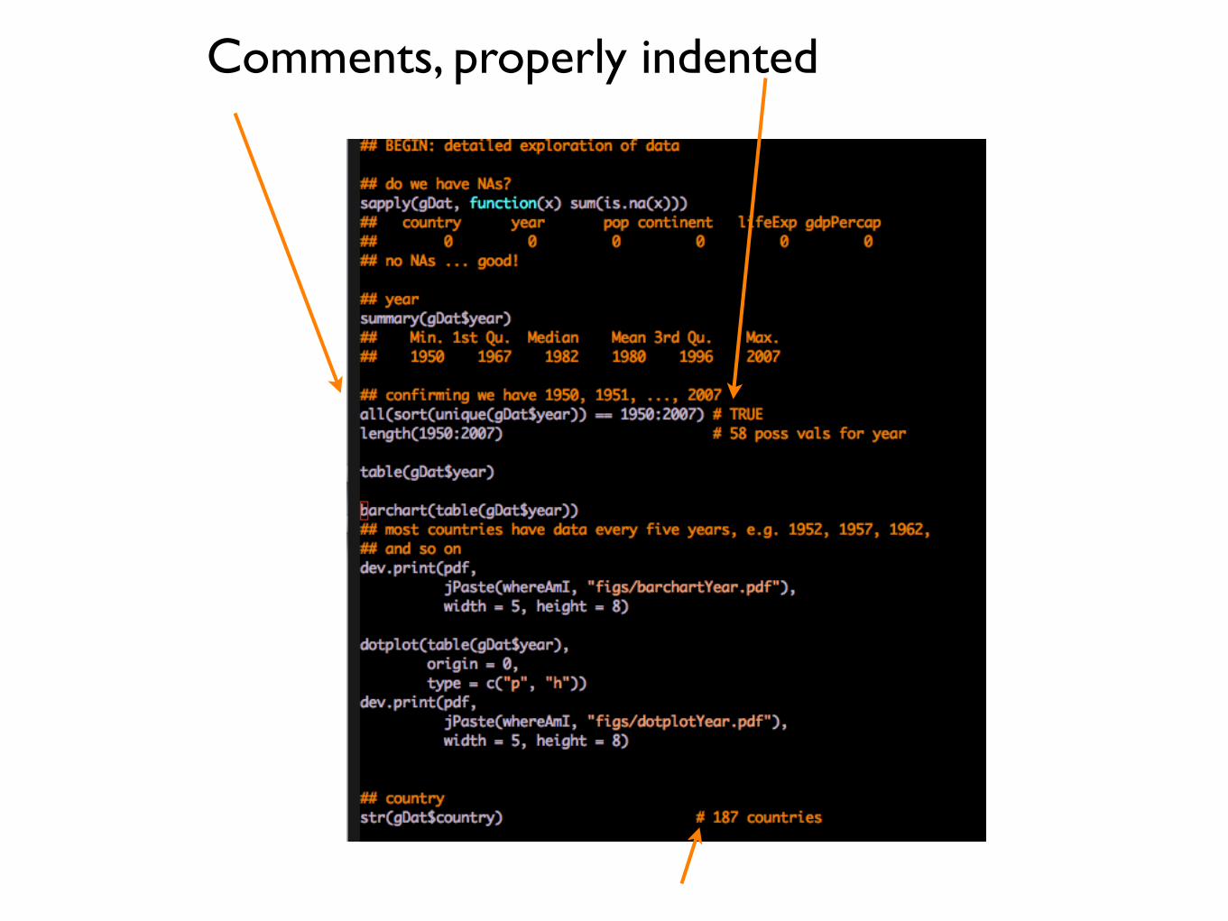
Comments, properly indented
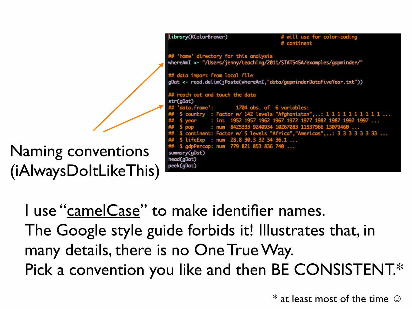
Naming conventions (iAlwaysDoItLikeThis)
I use “camelCase” to make identifier names.The Google style guide forbids it! Illustrates that, in many details, there is no One True Way.Pick a convention you like and then BE CONSISTENT.*
* at least most of the time ☺
Homework before next class:
Read at least two of the documents suggested about R style (or locate and suggest others!).
Develop a modest goal for partial implementation of “good” R style and start trying to achieve that.
Write a short blurb or review (a couple sentences is OK) about each piece you read, describing it or critiquing it or recounting how easy/hard/valuable/useless implementation seems to be. Is it about nitty-gritty code style or is it more about an approach programming? Is it fun or boring to read? You get the idea.
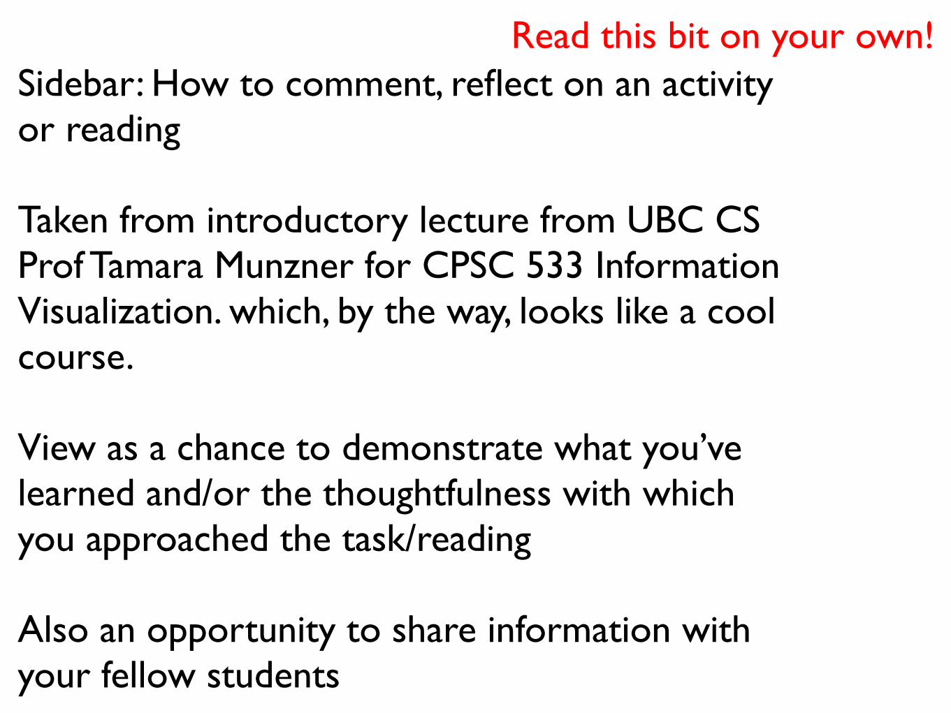
Sidebar: How to comment, reflect on an activity or reading
Taken from introductory lecture from UBC CS Prof Tamara Munzner for CPSC 533 Information Visualization. which, by the way, looks like a cool course.
View as a chance to demonstrate what you’ve learned and/or the thoughtfulness with which you approached the task/reading
Also an opportunity to share information with your fellow students
Read this bit on your own!
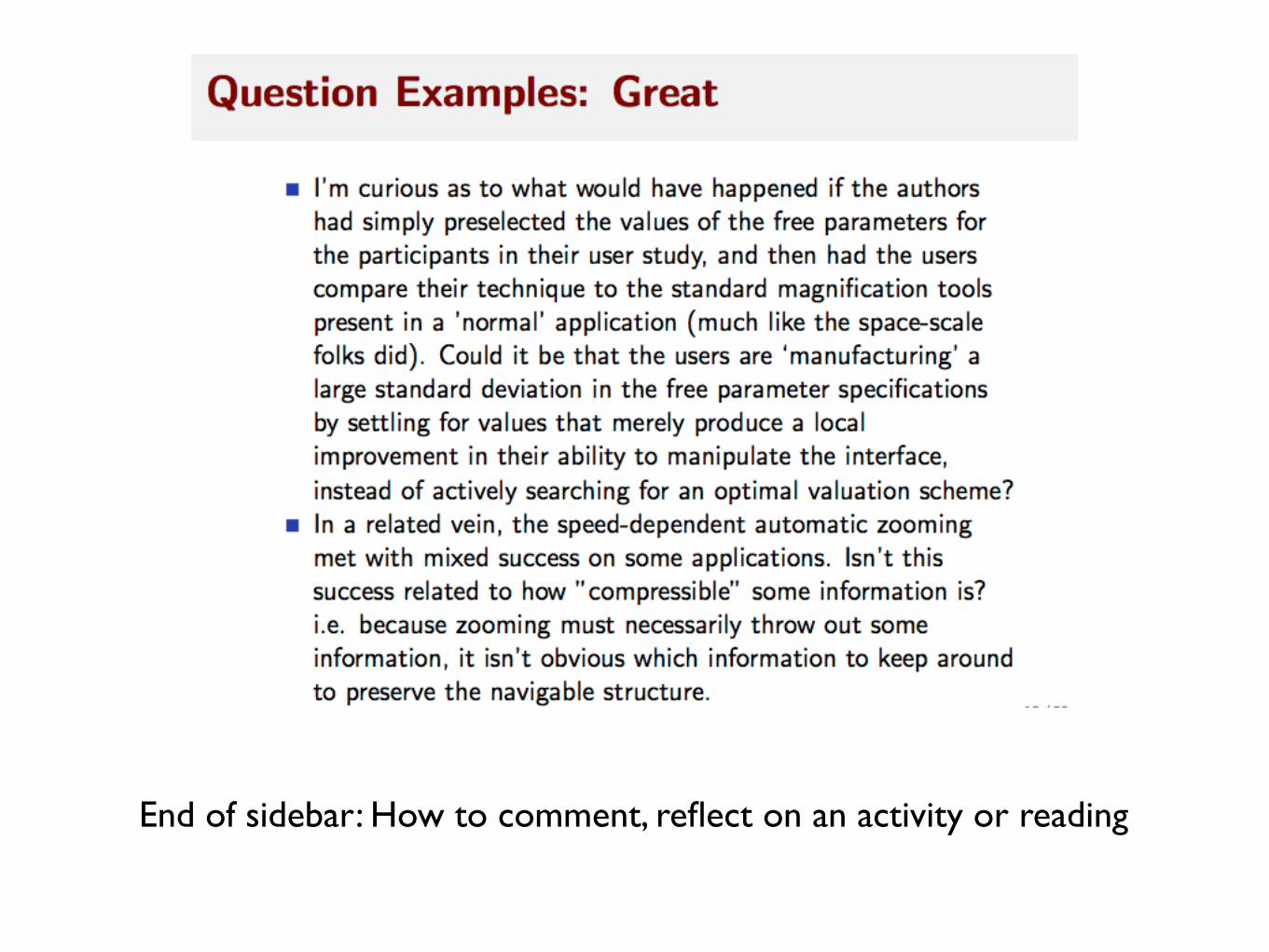
End of sidebar: How to comment, reflect on an activity or reading
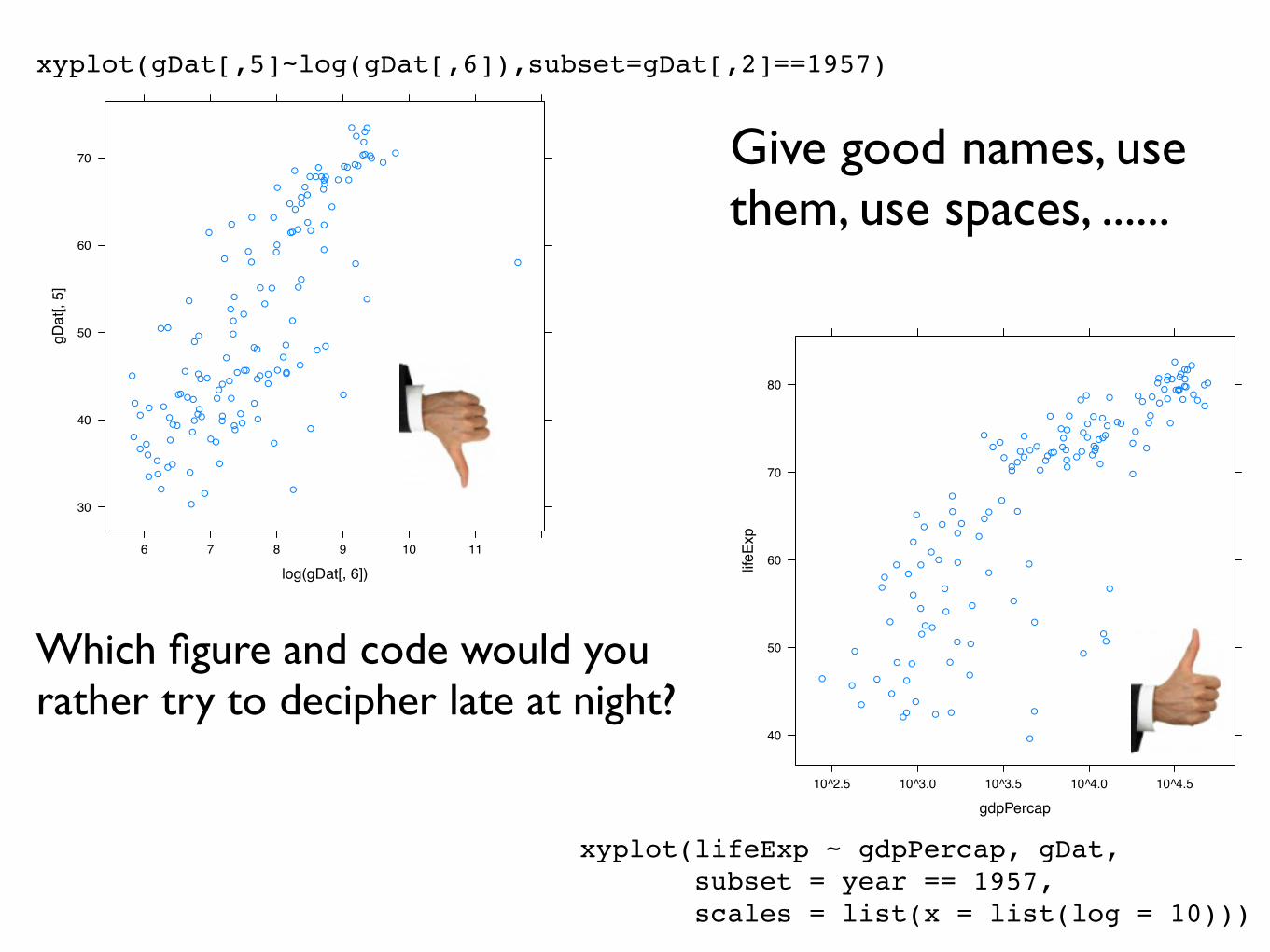
xyplot(gDat[,5]~log(gDat[,6]),subset=gDat[,2]==1957)
log(gDat[, 6])
gDat
[, 5]
30
40
50
60
70
6 7 8 9 10 11
●
●
●
●
●
●
●
●
●
●
●
●
●
●
●
●
●
●●
●
●
●
●
●
●
●
●
●
●
●
●
●
●
●
●
●
●
●
●
●
●
●
●
●
●
●
●
●
●
●
●
●●
●
●
●
●
●
● ●
●
●
●● ●
●
●
●●
●
●
●
●
●
●
●
●
●
●
●
●
●
●
●
●
●
●
●
●
●
●
●
●
●●
●
●
●
●
●
●
●
●
●
●
●
●
●
●
●
●
●
●
●
●●
●
●
●
●
●
●
●
●
●
●
●
●
●
●
●●
●
●●
●
●
●
●
●
●
●
xyplot(lifeExp ~ gdpPercap, gDat, subset = year == 1957, scales = list(x = list(log = 10)))
gdpPercap
lifeExp
40
50
60
70
80
10^2.5 10^3.0 10^3.5 10^4.0 10^4.5
●
●
●
●
●
●
●
●
●
●
●
●
●
●
●
●●●
●
●
●●
●
●
●
●
●
●
● ●
●
●
●
●
●
●
●
●
●
●
●
●●
●
●
●
●
●
●
●
●
●
●
●
●
●
●
●
●
●
●
●
●
●●
●
●
●
●
●
●
●
●
●
●
●●
●
●
●
●
●
●
●
●
●
●
●
●
●
●
●●
●
●
●
●
●
●
●
●
●
●
●●
●●
●
●
●
●
●
●
●
●
● ●
●
● ●
●
●
●
●
●
●
●
●
●
●
●
●
●
●
●
●
●●
●
●
●
●
Which figure and code would you rather try to decipher late at night?
Give good names, use them, use spaces, ......
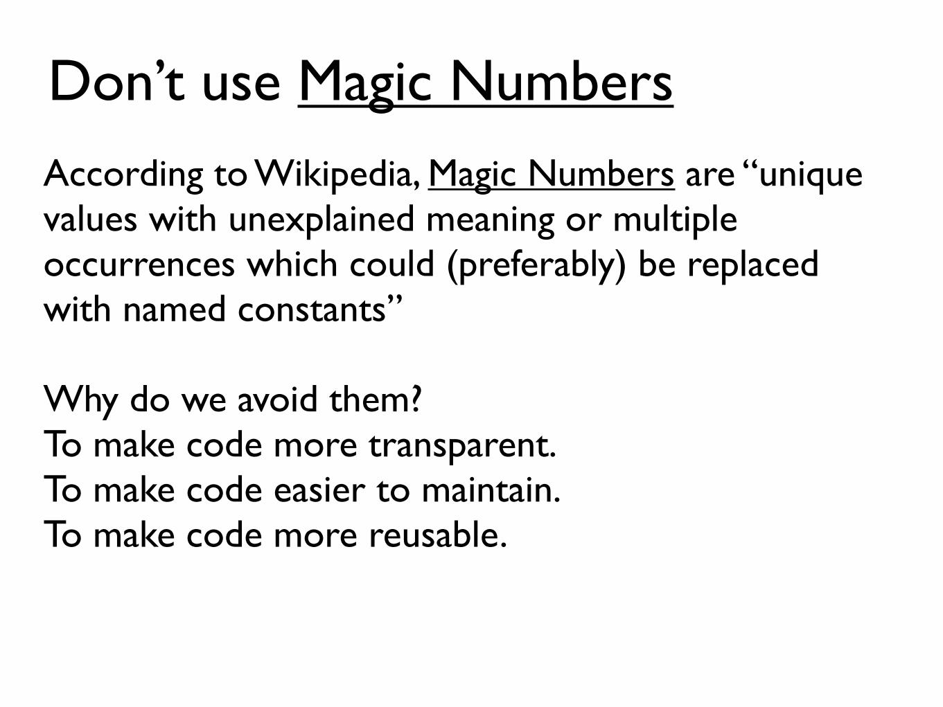
Don’t use Magic Numbers
According to Wikipedia, Magic Numbers are “unique values with unexplained meaning or multiple occurrences which could (preferably) be replaced with named constants”
Why do we avoid them?To make code more transparent.To make code easier to maintain.To make code more reusable.
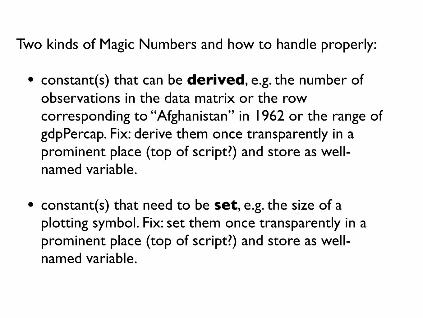
Two kinds of Magic Numbers and how to handle properly:
• constant(s) that can be derived, e.g. the number of observations in the data matrix or the row corresponding to “Afghanistan” in 1962 or the range of gdpPercap. Fix: derive them once transparently in a prominent place (top of script?) and store as well-named variable.
• constant(s) that need to be set, e.g. the size of a plotting symbol. Fix: set them once transparently in a prominent place (top of script?) and store as well-named variable.
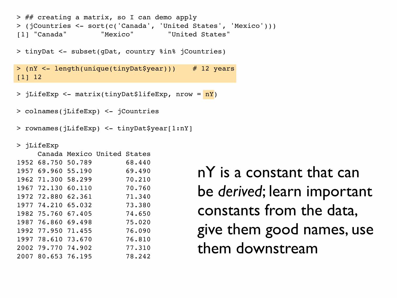
nY is a constant that can be derived; learn important constants from the data, give them good names, use them downstream
> ## creating a matrix, so I can demo apply> (jCountries <- sort(c('Canada', 'United States', 'Mexico')))[1] "Canada" "Mexico" "United States"
> tinyDat <- subset(gDat, country %in% jCountries)
> (nY <- length(unique(tinyDat$year))) # 12 years[1] 12
> jLifeExp <- matrix(tinyDat$lifeExp, nrow = nY)
> colnames(jLifeExp) <- jCountries
> rownames(jLifeExp) <- tinyDat$year[1:nY]
> jLifeExp Canada Mexico United States1952 68.750 50.789 68.4401957 69.960 55.190 69.4901962 71.300 58.299 70.2101967 72.130 60.110 70.7601972 72.880 62.361 71.3401977 74.210 65.032 73.3801982 75.760 67.405 74.6501987 76.860 69.498 75.0201992 77.950 71.455 76.0901997 78.610 73.670 76.8102002 79.770 74.902 77.3102007 80.653 76.195 78.242
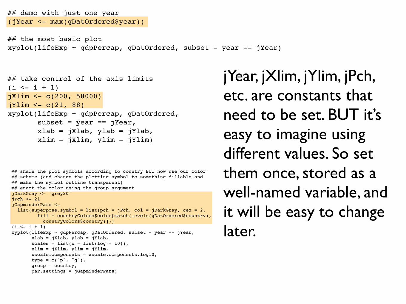
jYear, jXlim, jYlim, jPch, etc. are constants that need to be set. BUT it’s easy to imagine using different values. So set them once, stored as a well-named variable, and it will be easy to change later.
## demo with just one year(jYear <- max(gDatOrdered$year))
## the most basic plotxyplot(lifeExp ~ gdpPercap, gDatOrdered, subset = year == jYear)
## take control of the axis limits(i <- i + 1)jXlim <- c(200, 58000)jYlim <- c(21, 88)xyplot(lifeExp ~ gdpPercap, gDatOrdered, subset = year == jYear, xlab = jXlab, ylab = jYlab, xlim = jXlim, ylim = jYlim)
## shade the plot symbols according to country BUT now use our color## scheme (and change the plotting symbol to something fillable and## make the symbol outline transparent)## enact the color using the group argumentjDarkGray <- 'grey20'jPch <- 21jGapminderPars <- list(superpose.symbol = list(pch = jPch, col = jDarkGray, cex = 2, fill = countryColors$color[match(levels(gDatOrdered$country), countryColors$country)]))(i <- i + 1)xyplot(lifeExp ~ gdpPercap, gDatOrdered, subset = year == jYear, xlab = jXlab, ylab = jYlab, scales = list(x = list(log = 10)), xlim = jXlim, ylim = jYlim, xscale.components = xscale.components.log10, type = c("p", "g"), group = country, par.settings = jGapminderPars)
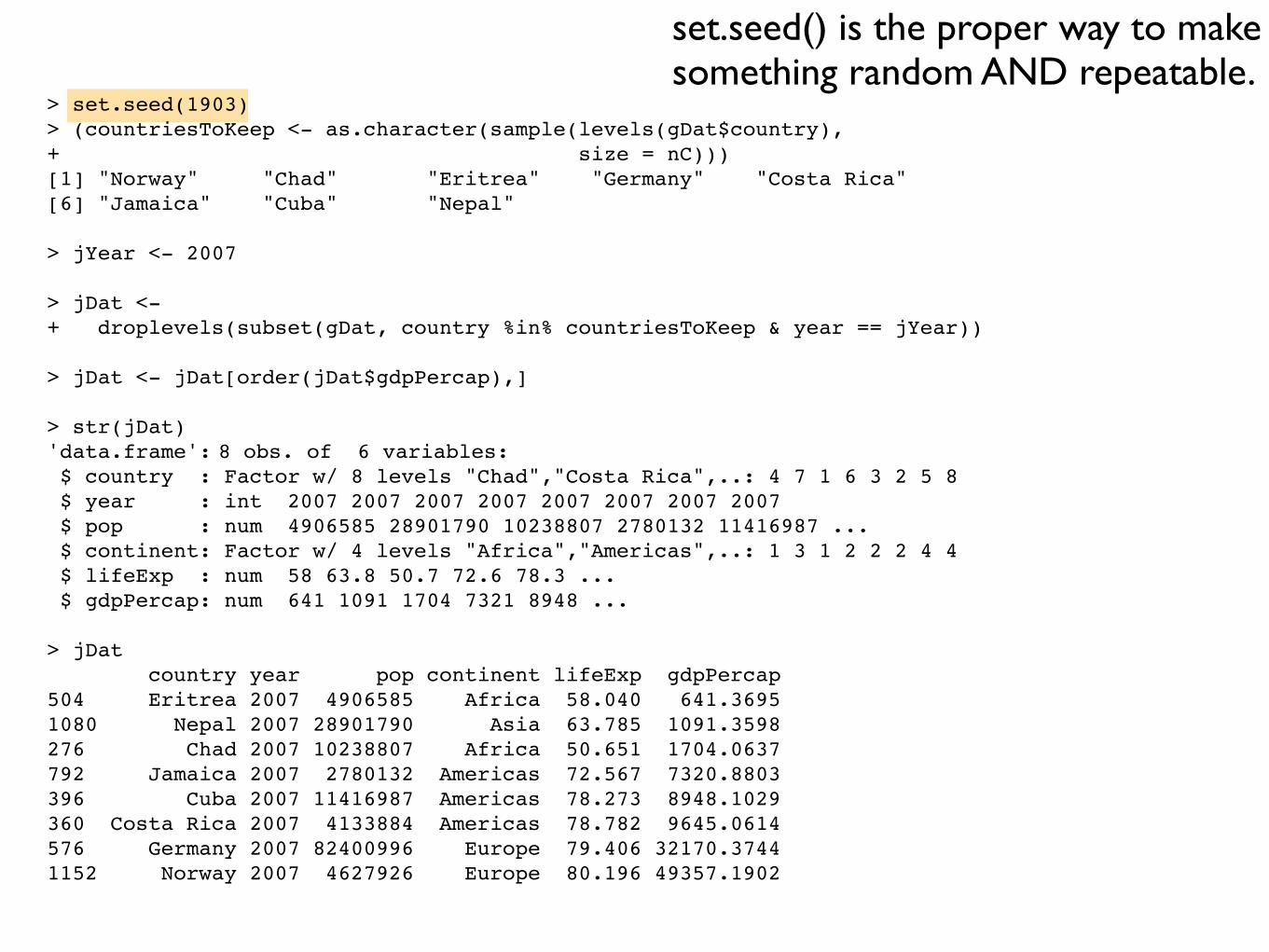
> set.seed(1903)> (countriesToKeep <- as.character(sample(levels(gDat$country),+ size = nC)))[1] "Norway" "Chad" "Eritrea" "Germany" "Costa Rica"[6] "Jamaica" "Cuba" "Nepal" > jYear <- 2007
> jDat <-+ droplevels(subset(gDat, country %in% countriesToKeep & year == jYear))
> jDat <- jDat[order(jDat$gdpPercap),]
> str(jDat)'data.frame':!8 obs. of 6 variables: $ country : Factor w/ 8 levels "Chad","Costa Rica",..: 4 7 1 6 3 2 5 8 $ year : int 2007 2007 2007 2007 2007 2007 2007 2007 $ pop : num 4906585 28901790 10238807 2780132 11416987 ... $ continent: Factor w/ 4 levels "Africa","Americas",..: 1 3 1 2 2 2 4 4 $ lifeExp : num 58 63.8 50.7 72.6 78.3 ... $ gdpPercap: num 641 1091 1704 7321 8948 ...
> jDat country year pop continent lifeExp gdpPercap504 Eritrea 2007 4906585 Africa 58.040 641.36951080 Nepal 2007 28901790 Asia 63.785 1091.3598276 Chad 2007 10238807 Africa 50.651 1704.0637792 Jamaica 2007 2780132 Americas 72.567 7320.8803396 Cuba 2007 11416987 Americas 78.273 8948.1029360 Costa Rica 2007 4133884 Americas 78.782 9645.0614576 Germany 2007 82400996 Europe 79.406 32170.37441152 Norway 2007 4627926 Europe 80.196 49357.1902
set.seed() is the proper way to make something random AND repeatable.
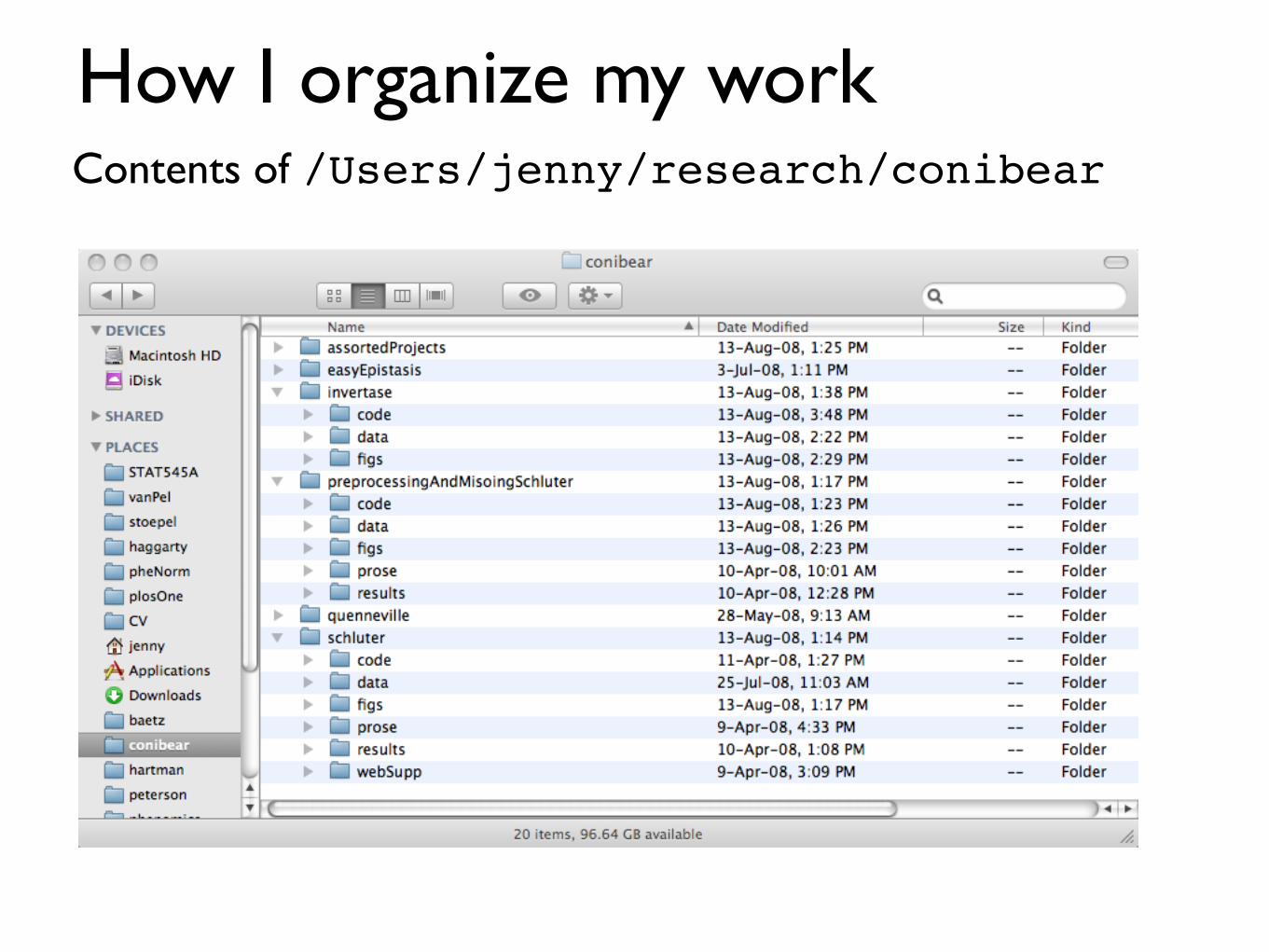
How I organize my workContents of /Users/jenny/research/conibear
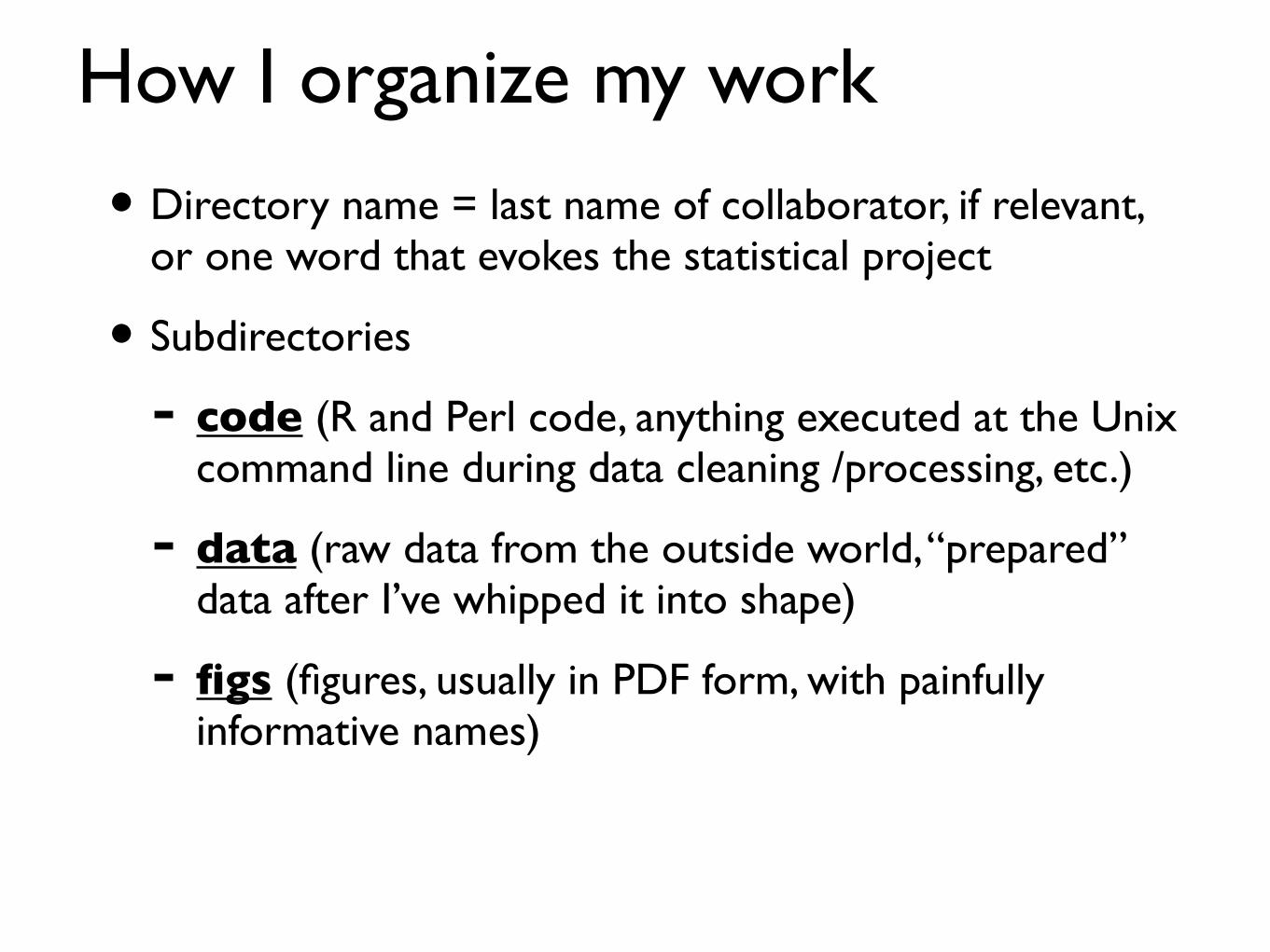
How I organize my work
• Directory name = last name of collaborator, if relevant, or one word that evokes the statistical project
• Subdirectories
- code (R and Perl code, anything executed at the Unix command line during data cleaning /processing, etc.)
- data (raw data from the outside world, “prepared” data after I’ve whipped it into shape)
- figs (figures, usually in PDF form, with painfully informative names)
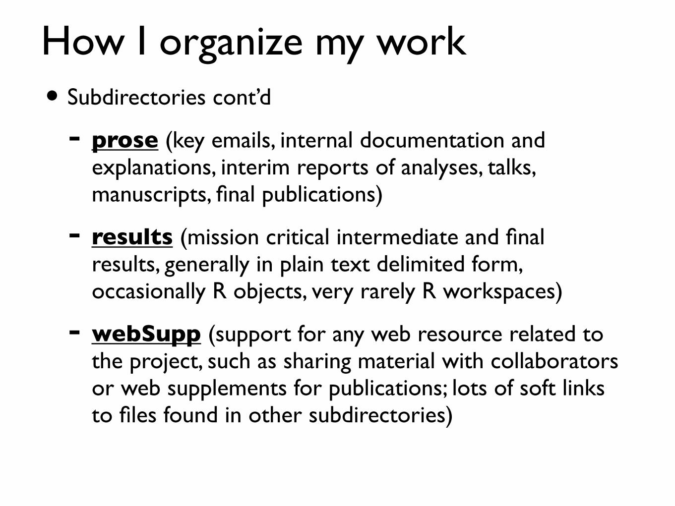
How I organize my work• Subdirectories cont’d
- prose (key emails, internal documentation and explanations, interim reports of analyses, talks, manuscripts, final publications)
- results (mission critical intermediate and final results, generally in plain text delimited form, occasionally R objects, very rarely R workspaces)
- webSupp (support for any web resource related to the project, such as sharing material with collaborators or web supplements for publications; lots of soft links to files found in other subdirectories)
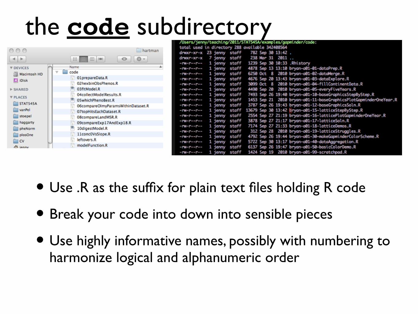
the code subdirectory
• Use .R as the suffix for plain text files holding R code
• Break your code into down into sensible pieces
• Use highly informative names, possibly with numbering to harmonize logical and alphanumeric order
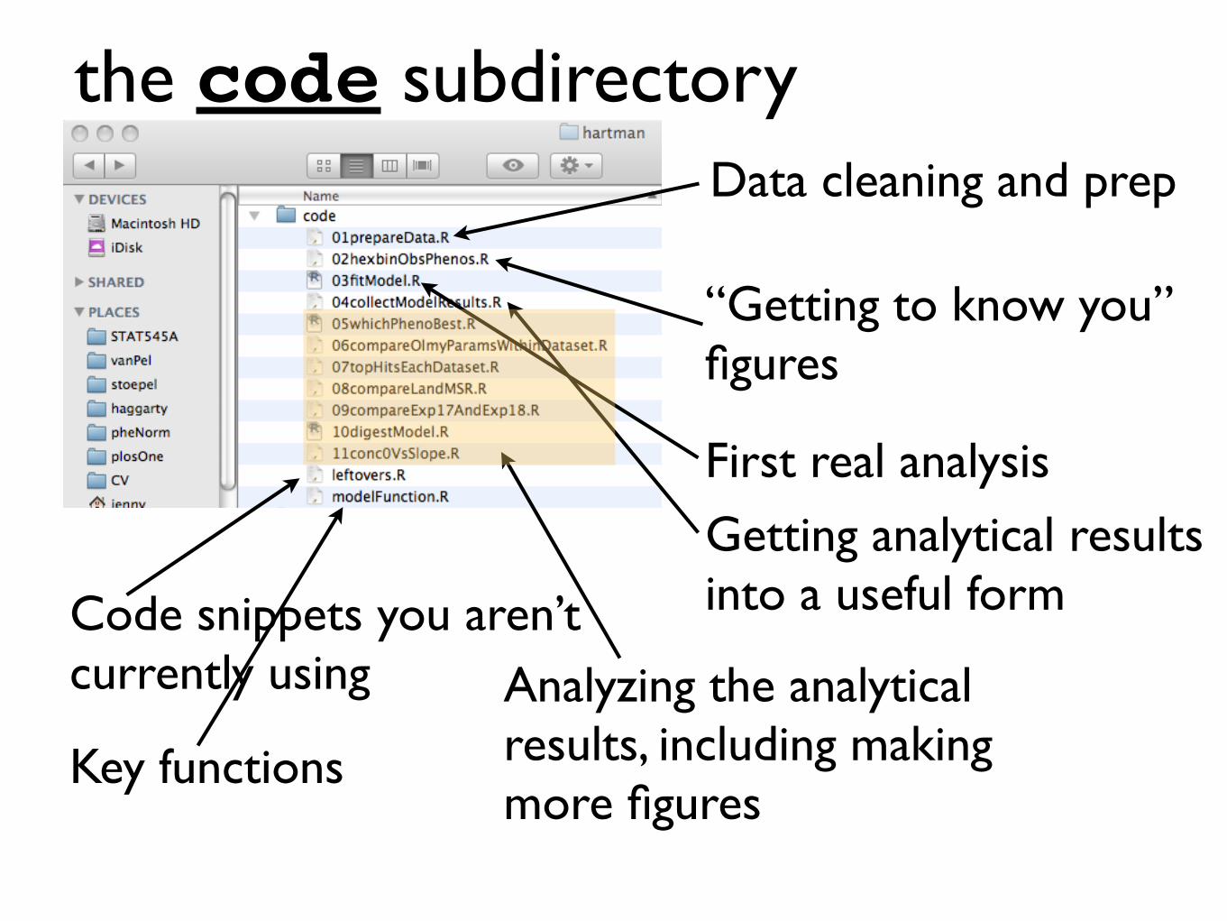
the code subdirectoryData cleaning and prep
“Getting to know you” figures
First real analysis
Getting analytical results into a useful form
Analyzing the analytical results, including making more figures
Key functions
Code snippets you aren’t currently using
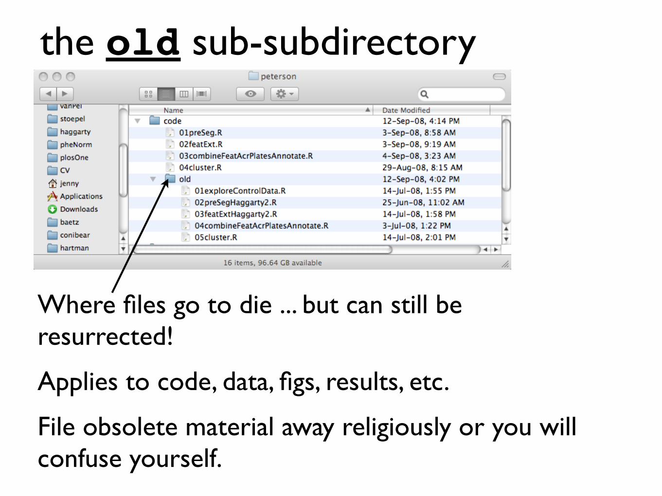
the old sub-subdirectory
Where files go to die ... but can still be resurrected!
Applies to code, data, figs, results, etc.
File obsolete material away religiously or you will confuse yourself.
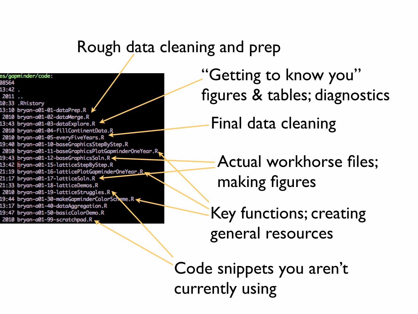
Rough data cleaning and prep
“Getting to know you” figures & tables; diagnostics
Final data cleaning
Actual workhorse files; making figures
Key functions; creating general resources
Code snippets you aren’t currently using
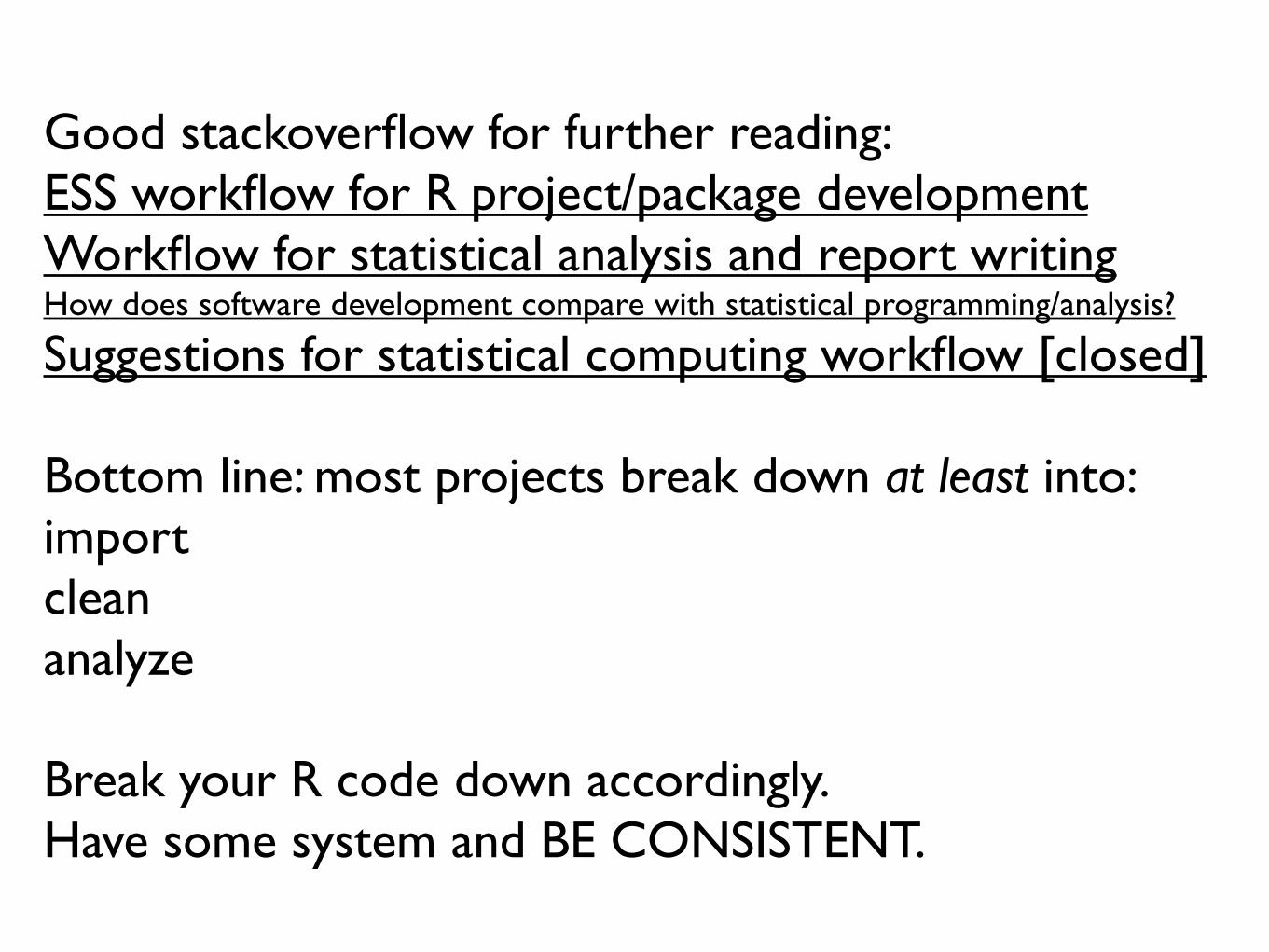
Good stackoverflow for further reading:ESS workflow for R project/package developmentWorkflow for statistical analysis and report writingHow does software development compare with statistical programming/analysis?
Suggestions for statistical computing workflow [closed]
Bottom line: most projects break down at least into:importcleananalyze
Break your R code down accordingly.Have some system and BE CONSISTENT.
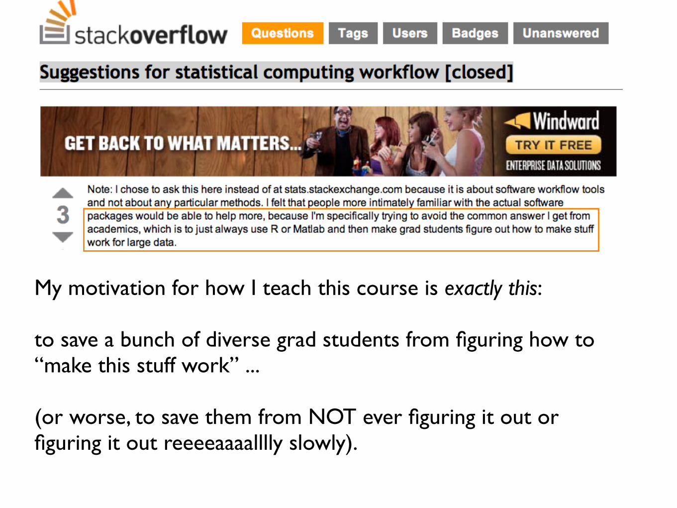
My motivation for how I teach this course is exactly this:
to save a bunch of diverse grad students from figuring how to “make this stuff work” ...
(or worse, to save them from NOT ever figuring it out or figuring it out reeeeaaaalllly slowly).
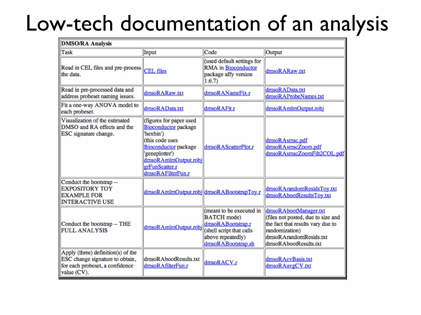
Low-tech documentation of an analysis
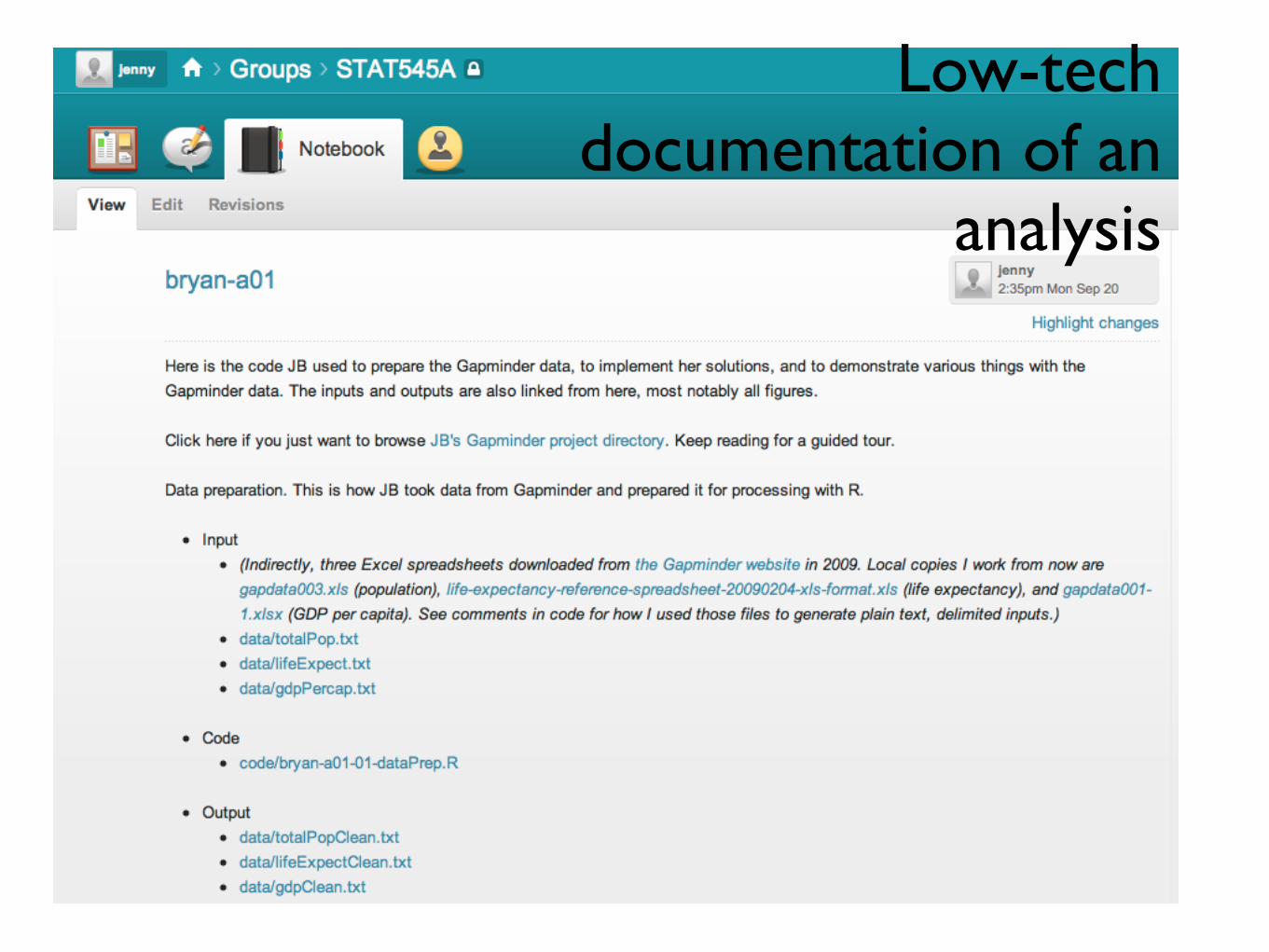
Low-tech documentation of an
analysis
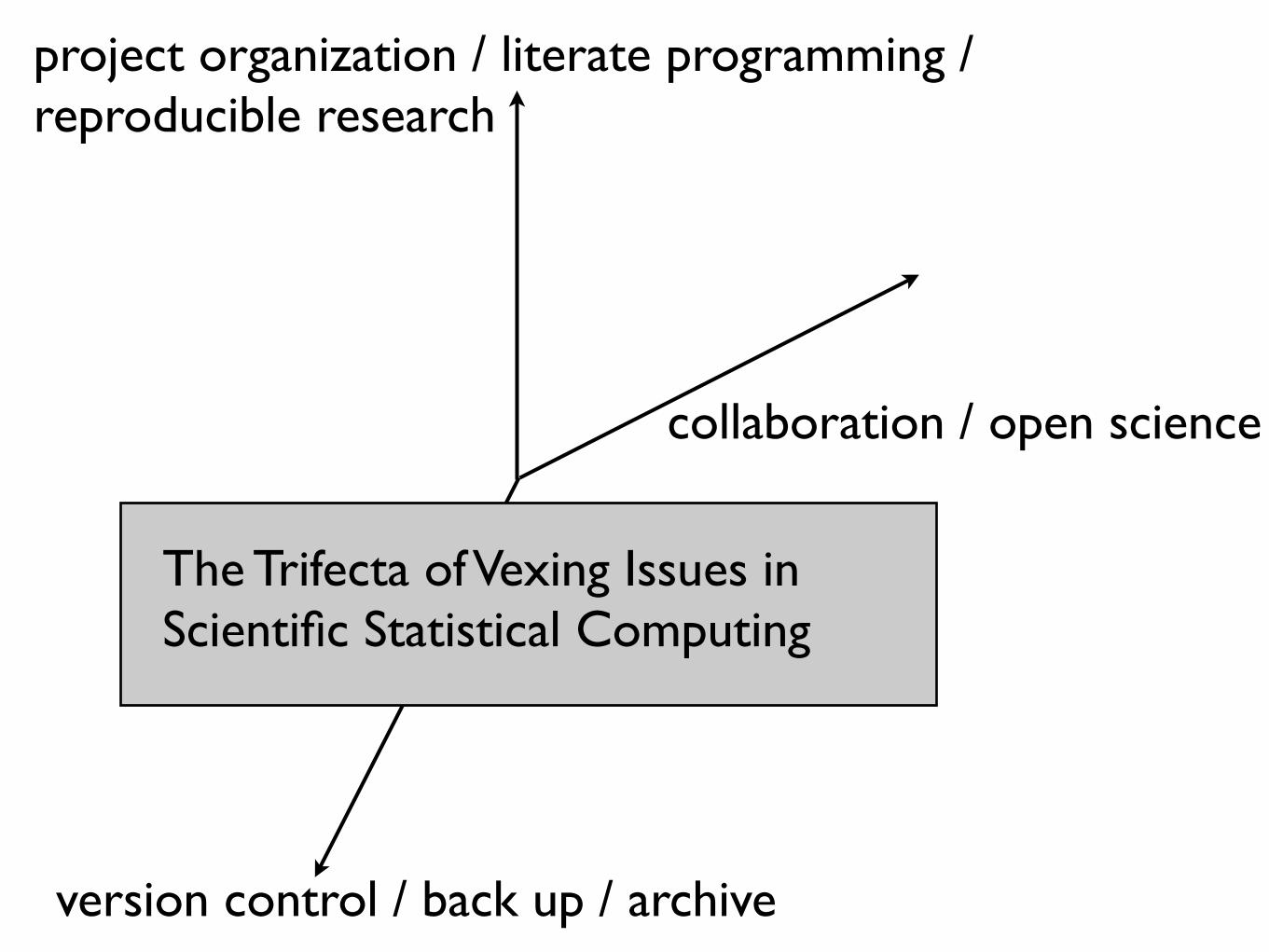
project organization / literate programming / reproducible research
version control / back up / archive
collaboration / open science
The Trifecta of Vexing Issues in Scientific Statistical Computing
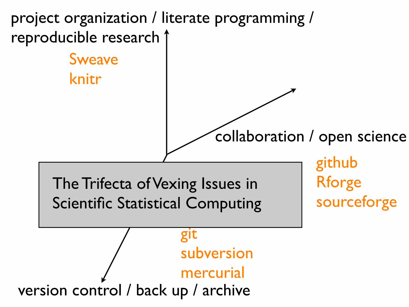
project organization / literate programming / reproducible research
version control / back up / archive
collaboration / open science
The Trifecta of Vexing Issues in Scientific Statistical Computing
Sweaveknitr
githubRforgesourceforge
gitsubversionmercurial

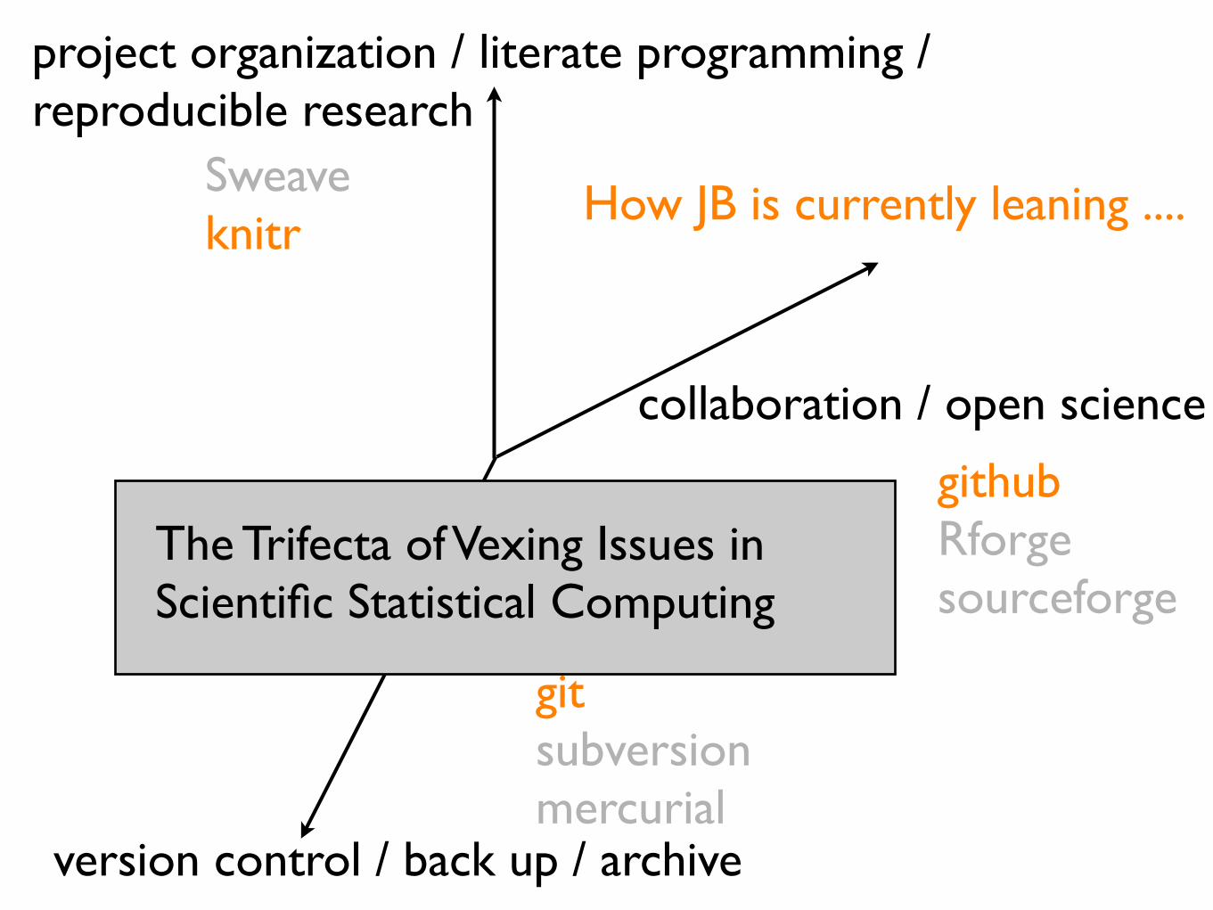
project organization / literate programming / reproducible research
version control / back up / archive
collaboration / open science
The Trifecta of Vexing Issues in Scientific Statistical Computing
Sweaveknitr
githubRforgesourceforge
gitsubversionmercurial
How JB is currently leaning ....
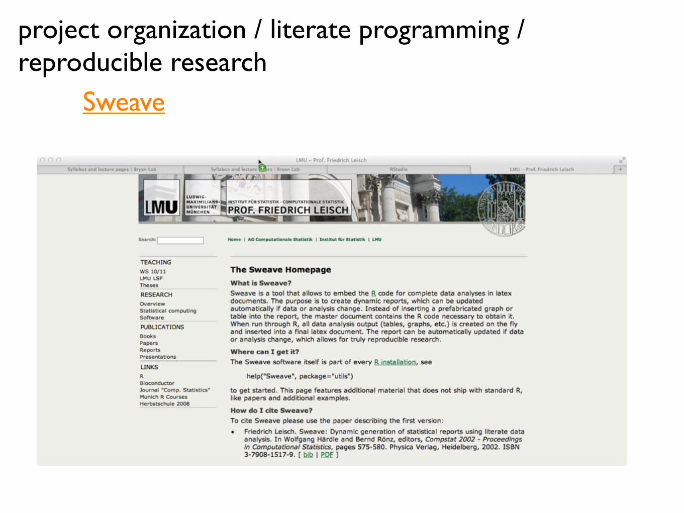
project organization / literate programming / reproducible research
Sweave
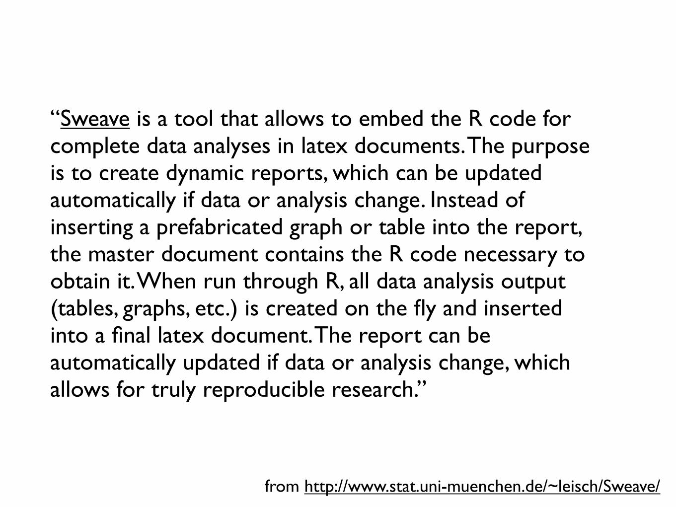
“Sweave is a tool that allows to embed the R code for complete data analyses in latex documents. The purpose is to create dynamic reports, which can be updated automatically if data or analysis change. Instead of inserting a prefabricated graph or table into the report, the master document contains the R code necessary to obtain it. When run through R, all data analysis output (tables, graphs, etc.) is created on the fly and inserted into a final latex document. The report can be automatically updated if data or analysis change, which allows for truly reproducible research.”
from http://www.stat.uni-muenchen.de/~leisch/Sweave/
project organization / literate programming / reproducible research
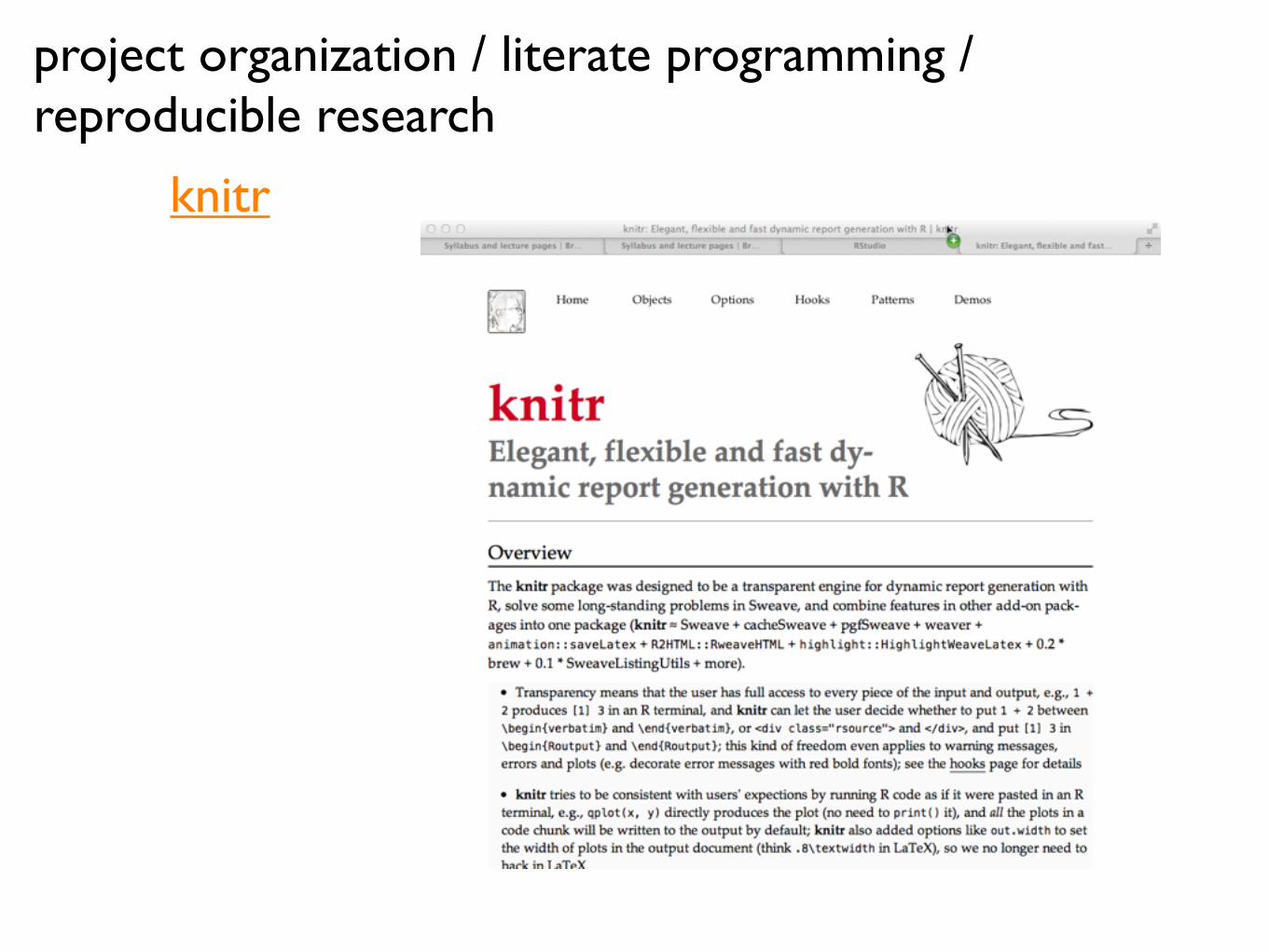
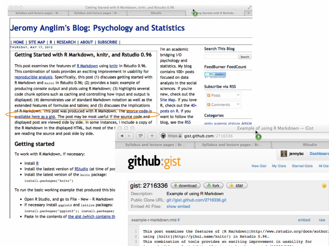
knitr
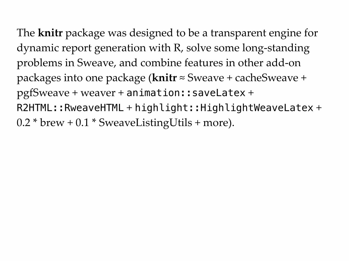
The knitr package was designed to be a transparent engine for dynamic report generation with R, solve some long-‐‑standing problems in Sweave, and combine features in other add-‐‑on packages into one package (knitr ≈ Sweave + cacheSweave + pgfSweave + weaver + animation::saveLatex + R2HTML::RweaveHTML + highlight::HighlightWeaveLatex + 0.2 * brew + 0.1 * SweaveListingUtils + more).
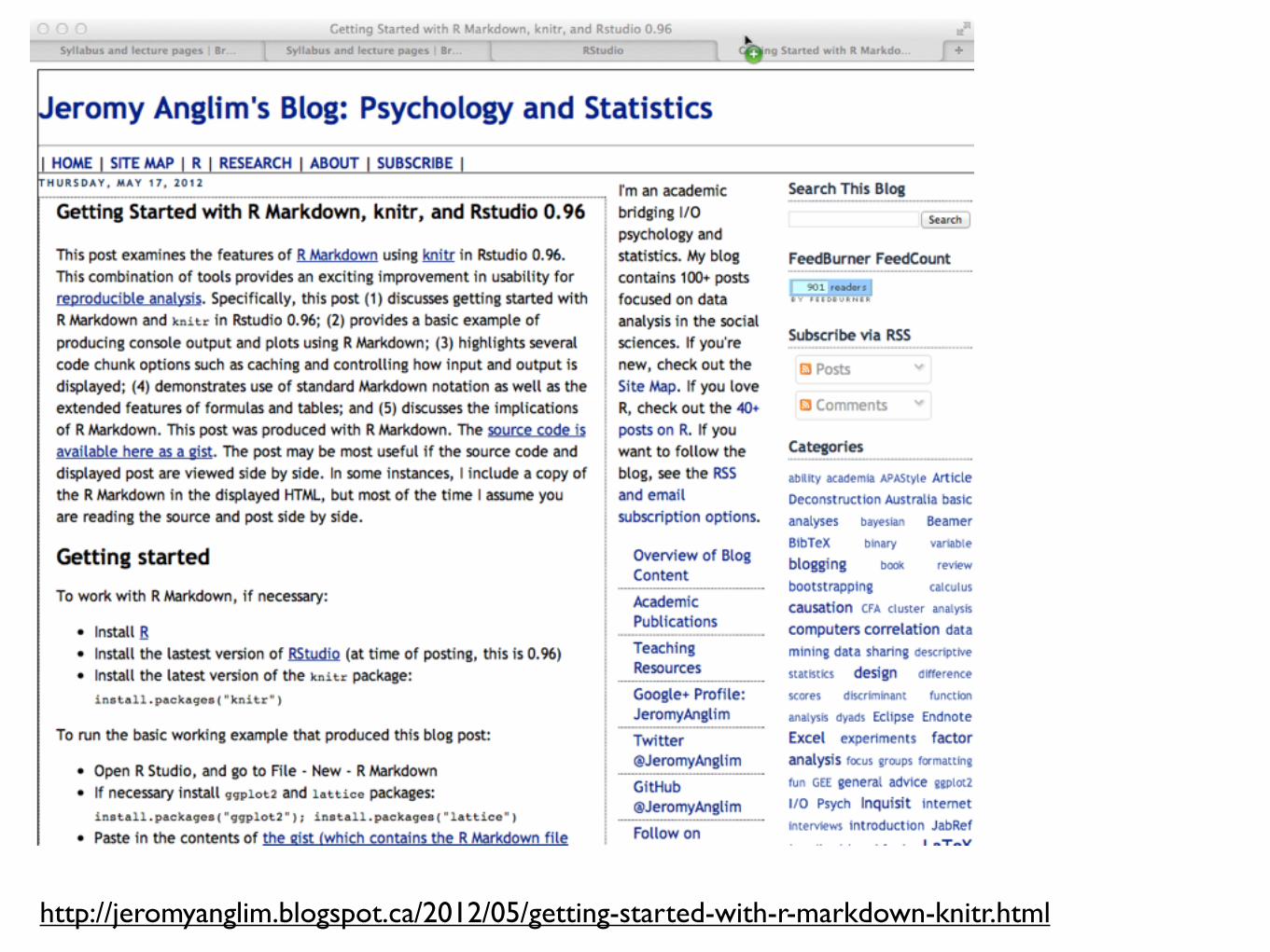
http://jeromyanglim.blogspot.ca/2012/05/getting-started-with-r-markdown-knitr.html
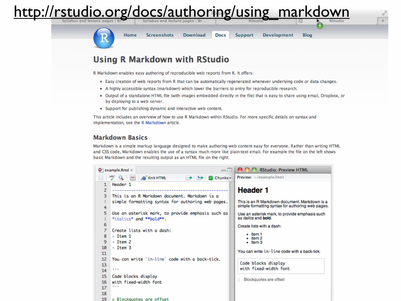
http://rstudio.org/docs/authoring/using_markdown
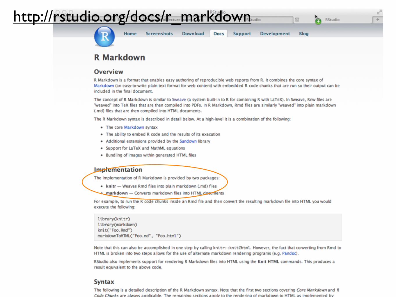
http://rstudio.org/docs/r_markdown

project organization / literate programming / reproducible research
version control / back up / archive
collaboration / open science
The Trifecta of Vexing Issues in Scientific Statistical Computing
Sweaveknitr
githubRforgesourceforge
gitsubversionmercurial
How JB is currently leaning ....
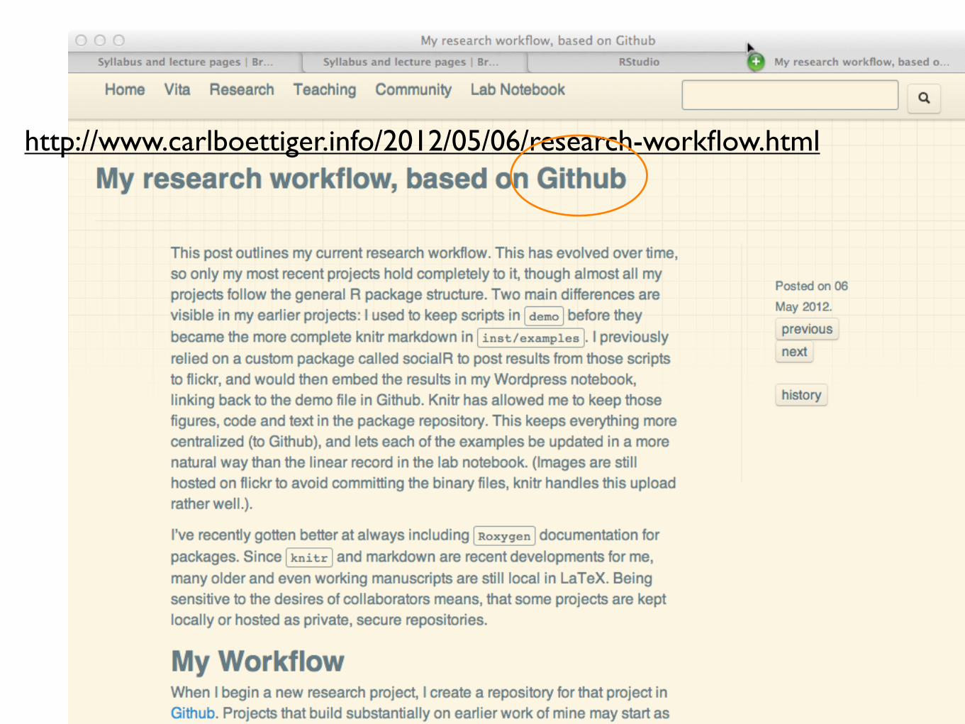
http://www.carlboettiger.info/2012/05/06/research-workflow.html
project organization / literate programming / reproducible research
version control / back up / archive
collaboration / open science
The Trifecta of Vexing Issues in Scientific Statistical Computing
Sweaveknitr
githubRforgesourceforge
gitsubversionmercurial
How JB is currently leaning ....
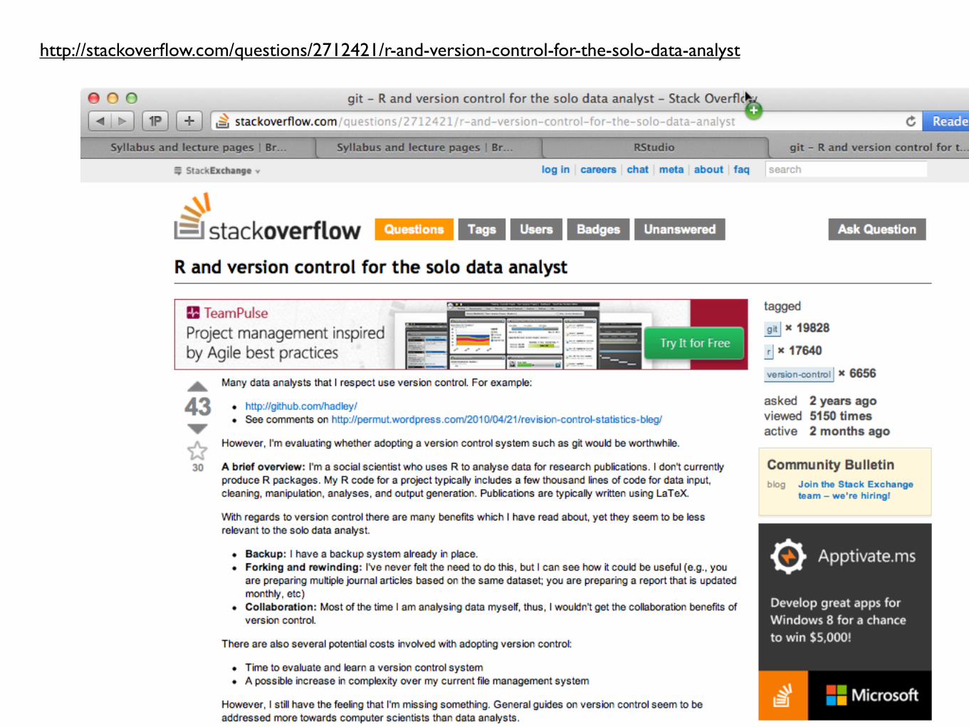
http://stackoverflow.com/questions/2712421/r-and-version-control-for-the-solo-data-analyst
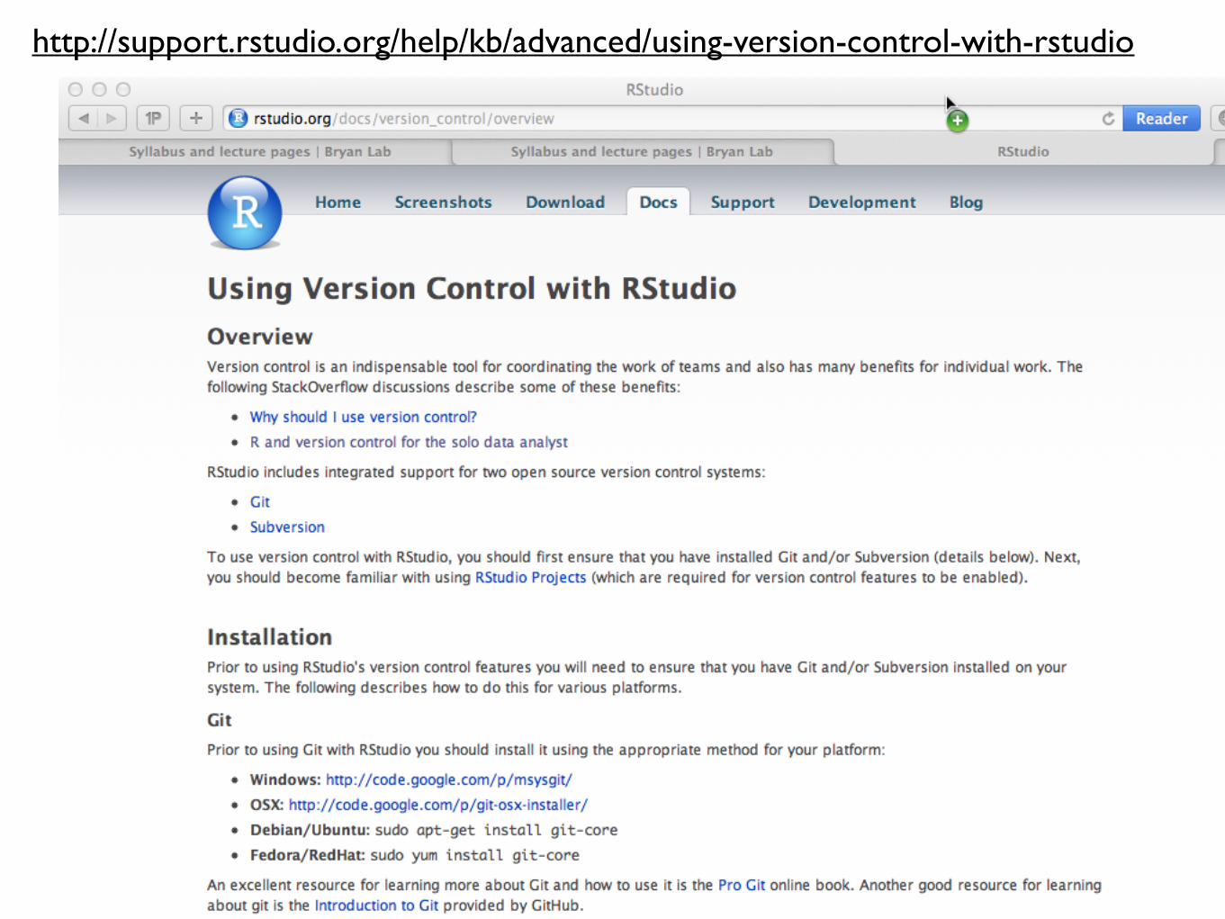
http://support.rstudio.org/help/kb/advanced/using-version-control-with-rstudio

project organization / literate programming / reproducible research
version control / back up / archive
collaboration / open science
The Trifecta of Vexing Issues in Scientific Statistical Computing
Sweaveknitr
githubRforgesourceforge
gitsubversionmercurial
How JB is currently leaning ....
Bottom line: do something deliberate that has a good hassle: result ratio for you.
Be open to upgrading your approach as time goes on.
Keep your eyes and ears open re: developments in this area!
Your R life, in general
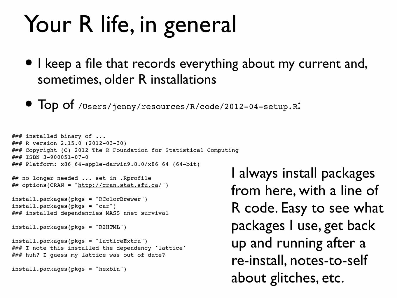
• I keep a file that records everything about my current and, sometimes, older R installations
• Top of /Users/jenny/resources/R/code/2012-04-setup.R:
### installed binary of ...### R version 2.15.0 (2012-03-30)### Copyright (C) 2012 The R Foundation for Statistical Computing### ISBN 3-900051-07-0### Platform: x86_64-apple-darwin9.8.0/x86_64 (64-bit)
## no longer needed ... set in .Rprofile## options(CRAN = "http://cran.stat.sfu.ca/")
install.packages(pkgs = "RColorBrewer")install.packages(pkgs = "car")### installed dependencies MASS nnet survival
install.packages(pkgs = "R2HTML")
install.packages(pkgs = "latticeExtra")### I note this installed the dependency 'lattice'### huh? I guess my lattice was out of date?
install.packages(pkgs = "hexbin")
I always install packages from here, with a line of R code. Easy to see what packages I use, get back up and running after a re-install, notes-to-self about glitches, etc.
Your R life, in general
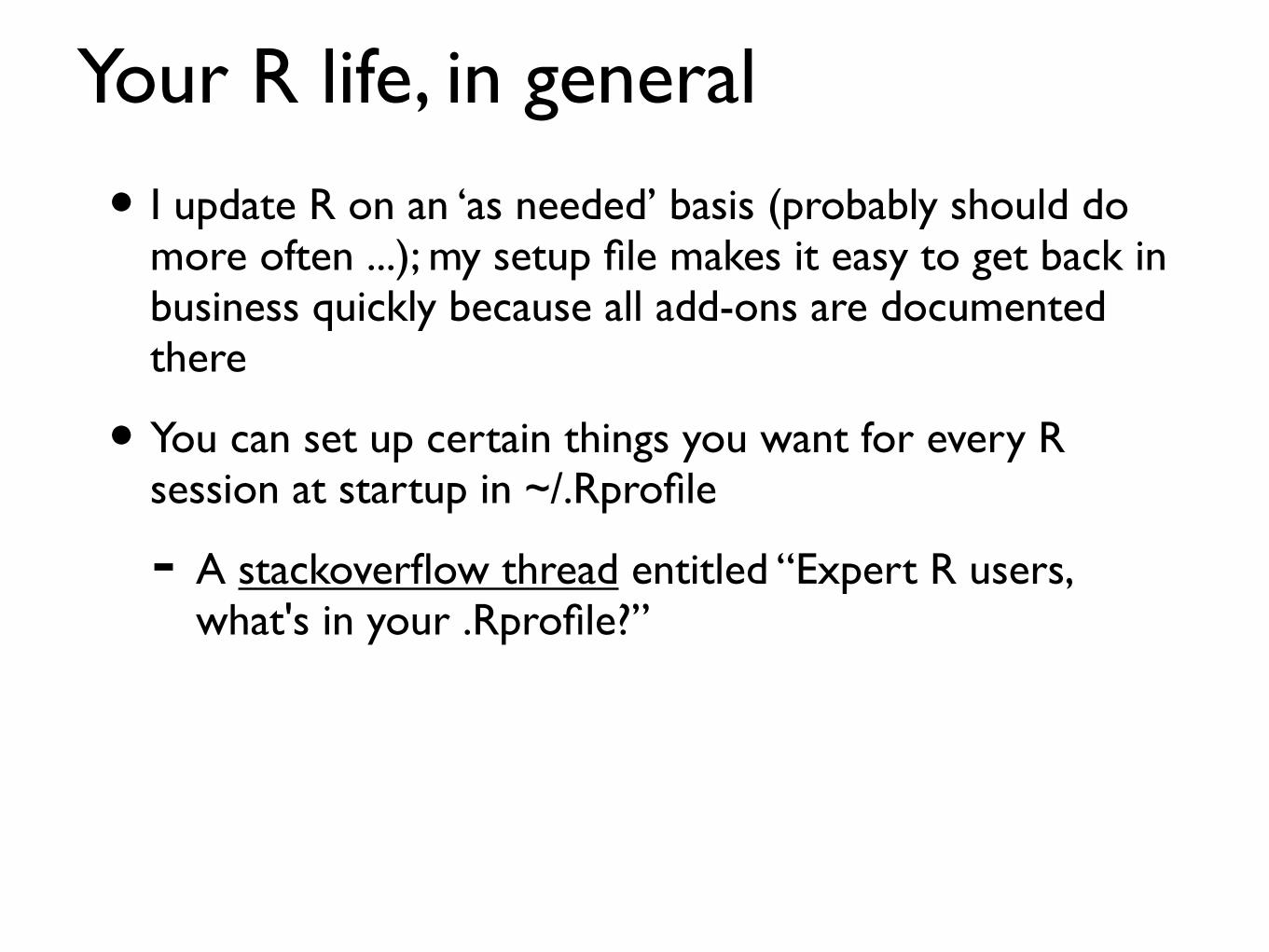
• I update R on an ‘as needed’ basis (probably should do more often ...); my setup file makes it easy to get back in business quickly because all add-ons are documented there
• You can set up certain things you want for every R session at startup in ~/.Rprofile
- A stackoverflow thread entitled “Expert R users, what's in your .Rprofile?”
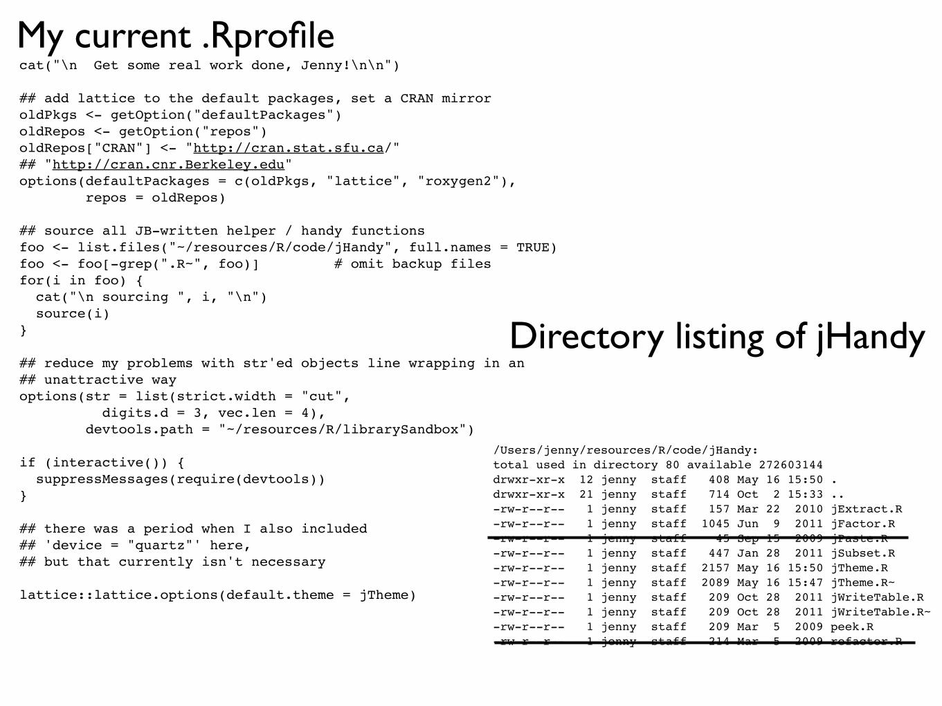
cat("\n Get some real work done, Jenny!\n\n")
## add lattice to the default packages, set a CRAN mirroroldPkgs <- getOption("defaultPackages")oldRepos <- getOption("repos")oldRepos["CRAN"] <- "http://cran.stat.sfu.ca/"## "http://cran.cnr.Berkeley.edu"options(defaultPackages = c(oldPkgs, "lattice", "roxygen2"), repos = oldRepos)
## source all JB-written helper / handy functionsfoo <- list.files("~/resources/R/code/jHandy", full.names = TRUE)foo <- foo[-grep(".R~", foo)] # omit backup filesfor(i in foo) { cat("\n sourcing ", i, "\n") source(i)}
## reduce my problems with str'ed objects line wrapping in an## unattractive wayoptions(str = list(strict.width = "cut", digits.d = 3, vec.len = 4), devtools.path = "~/resources/R/librarySandbox")
if (interactive()) { suppressMessages(require(devtools))}
## there was a period when I also included## 'device = "quartz"' here,## but that currently isn't necessary
lattice::lattice.options(default.theme = jTheme)
My current .Rprofile
/Users/jenny/resources/R/code/jHandy: total used in directory 80 available 272603144 drwxr-xr-x 12 jenny staff 408 May 16 15:50 . drwxr-xr-x 21 jenny staff 714 Oct 2 15:33 .. -rw-r--r-- 1 jenny staff 157 Mar 22 2010 jExtract.R -rw-r--r-- 1 jenny staff 1045 Jun 9 2011 jFactor.R -rw-r--r-- 1 jenny staff 45 Sep 15 2009 jPaste.R -rw-r--r-- 1 jenny staff 447 Jan 28 2011 jSubset.R -rw-r--r-- 1 jenny staff 2157 May 16 15:50 jTheme.R -rw-r--r-- 1 jenny staff 2089 May 16 15:47 jTheme.R~ -rw-r--r-- 1 jenny staff 209 Oct 28 2011 jWriteTable.R -rw-r--r-- 1 jenny staff 209 Oct 28 2011 jWriteTable.R~ -rw-r--r-- 1 jenny staff 209 Mar 5 2009 peek.R -rw-r--r-- 1 jenny staff 214 Mar 5 2009 refactor.R
Directory listing of jHandy
Full disclosure: one should probably convert personal functions that are used throughout your code into a proper R package .....
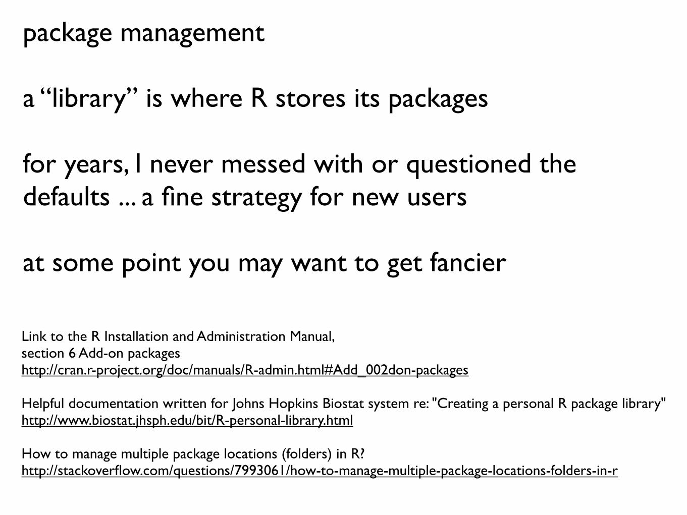
package management
a “library” is where R stores its packages
for years, I never messed with or questioned the defaults ... a fine strategy for new users
at some point you may want to get fancier
Link to the R Installation and Administration Manual,section 6 Add-on packageshttp://cran.r-project.org/doc/manuals/R-admin.html#Add_002don-packages
Helpful documentation written for Johns Hopkins Biostat system re: "Creating a personal R package library"http://www.biostat.jhsph.edu/bit/R-personal-library.html
How to manage multiple package locations (folders) in R?http://stackoverflow.com/questions/7993061/how-to-manage-multiple-package-locations-folders-in-r
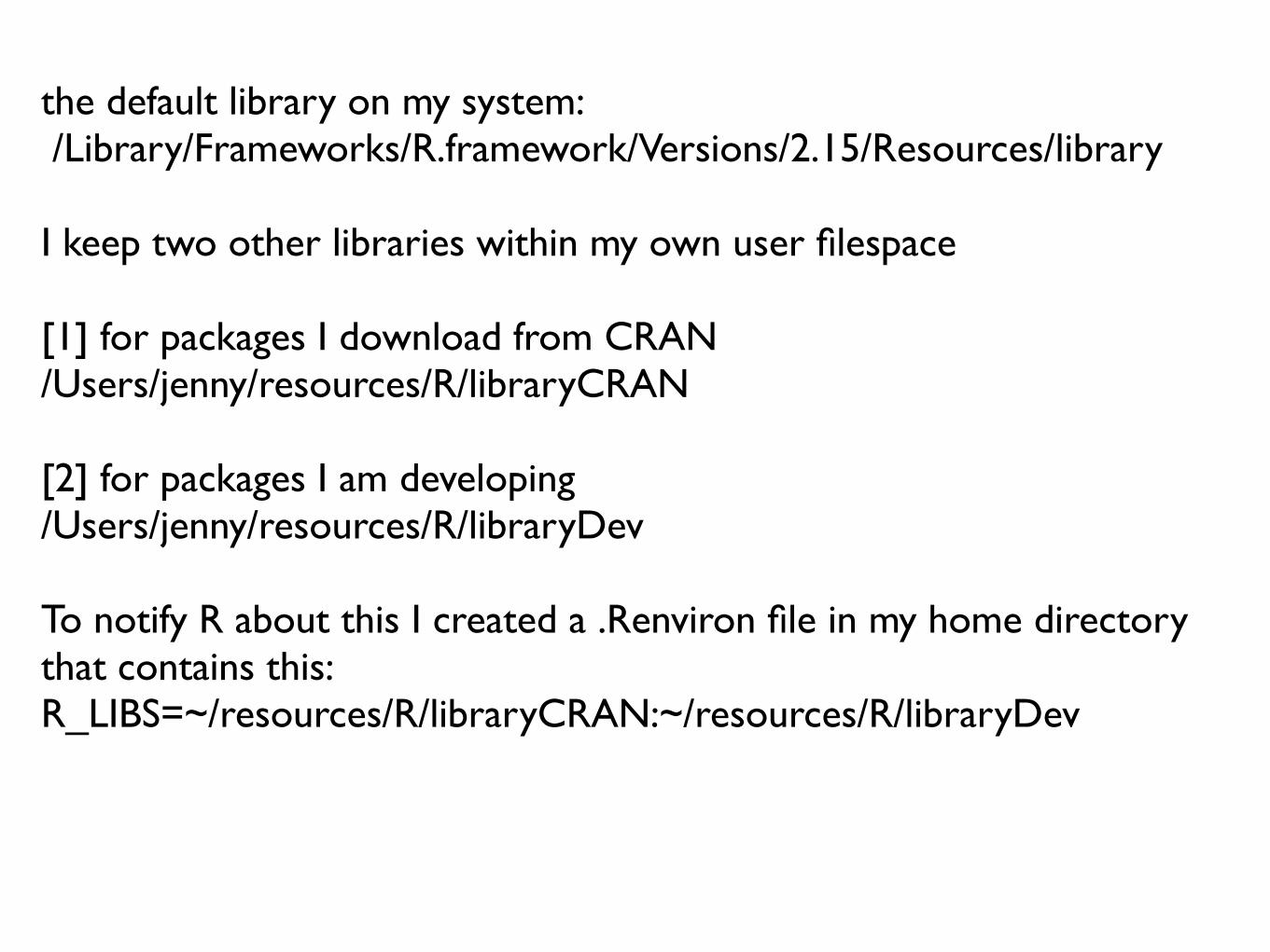
the default library on my system: /Library/Frameworks/R.framework/Versions/2.15/Resources/library
I keep two other libraries within my own user filespace
[1] for packages I download from CRAN/Users/jenny/resources/R/libraryCRAN
[2] for packages I am developing/Users/jenny/resources/R/libraryDev
To notify R about this I created a .Renviron file in my home directory that contains this:R_LIBS=~/resources/R/libraryCRAN:~/resources/R/libraryDev
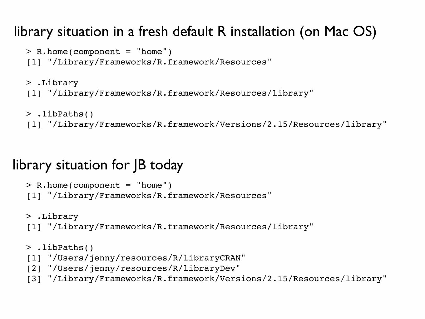
> R.home(component = "home")[1] "/Library/Frameworks/R.framework/Resources"
> .Library[1] "/Library/Frameworks/R.framework/Resources/library"
> .libPaths()[1] "/Library/Frameworks/R.framework/Versions/2.15/Resources/library"
library situation in a fresh default R installation (on Mac OS)
> R.home(component = "home")[1] "/Library/Frameworks/R.framework/Resources"
> .Library[1] "/Library/Frameworks/R.framework/Resources/library"
> .libPaths()[1] "/Users/jenny/resources/R/libraryCRAN" [2] "/Users/jenny/resources/R/libraryDev" [3] "/Library/Frameworks/R.framework/Versions/2.15/Resources/library"
library situation for JB today
Getting data out of R
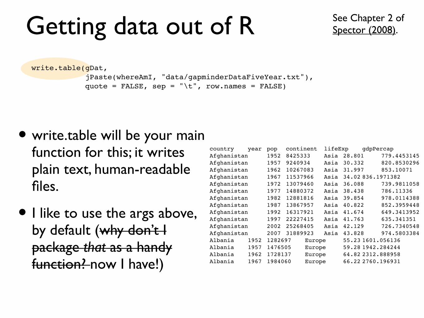
• write.table will be your main function for this; it writes plain text, human-readable files.
• I like to use the args above, by default (why don’t I package that as a handy function? now I have!)
See Chapter 2 of Spector (2008).
write.table(gDat, jPaste(whereAmI, "data/gapminderDataFiveYear.txt"), quote = FALSE, sep = "\t", row.names = FALSE)
country! year! pop! continent! lifeExp! gdpPercapAfghanistan! 1952! 8425333! Asia! 28.801! 779.4453145Afghanistan! 1957! 9240934! Asia! 30.332! 820.8530296Afghanistan! 1962! 10267083! Asia! 31.997! 853.10071Afghanistan! 1967! 11537966! Asia! 34.02!836.1971382Afghanistan! 1972! 13079460! Asia! 36.088! 739.9811058Afghanistan! 1977! 14880372! Asia! 38.438! 786.11336Afghanistan! 1982! 12881816! Asia! 39.854! 978.0114388Afghanistan! 1987! 13867957! Asia! 40.822! 852.3959448Afghanistan! 1992! 16317921! Asia! 41.674! 649.3413952Afghanistan! 1997! 22227415! Asia! 41.763! 635.341351Afghanistan! 2002! 25268405! Asia! 42.129! 726.7340548Afghanistan! 2007! 31889923! Asia! 43.828! 974.5803384Albania! 1952! 1282697! Europe! 55.23!1601.056136Albania! 1957! 1476505! Europe! 59.28!1942.284244Albania! 1962! 1728137! Europe! 64.82!2312.888958Albania! 1967! 1984060! Europe! 66.22!2760.196931
Getting data out of R
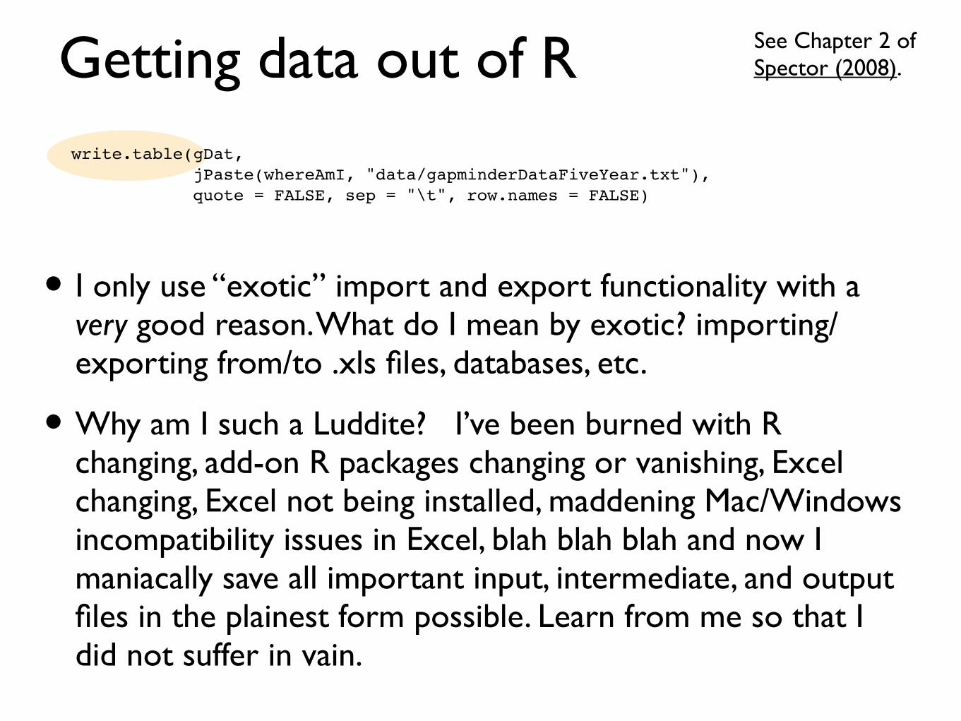
• I only use “exotic” import and export functionality with a very good reason. What do I mean by exotic? importing/exporting from/to .xls files, databases, etc.
• Why am I such a Luddite? I’ve been burned with R changing, add-on R packages changing or vanishing, Excel changing, Excel not being installed, maddening Mac/Windows incompatibility issues in Excel, blah blah blah and now I maniacally save all important input, intermediate, and output files in the plainest form possible. Learn from me so that I did not suffer in vain.
See Chapter 2 of Spector (2008).
write.table(gDat, jPaste(whereAmI, "data/gapminderDataFiveYear.txt"), quote = FALSE, sep = "\t", row.names = FALSE)
Getting stuff out of R
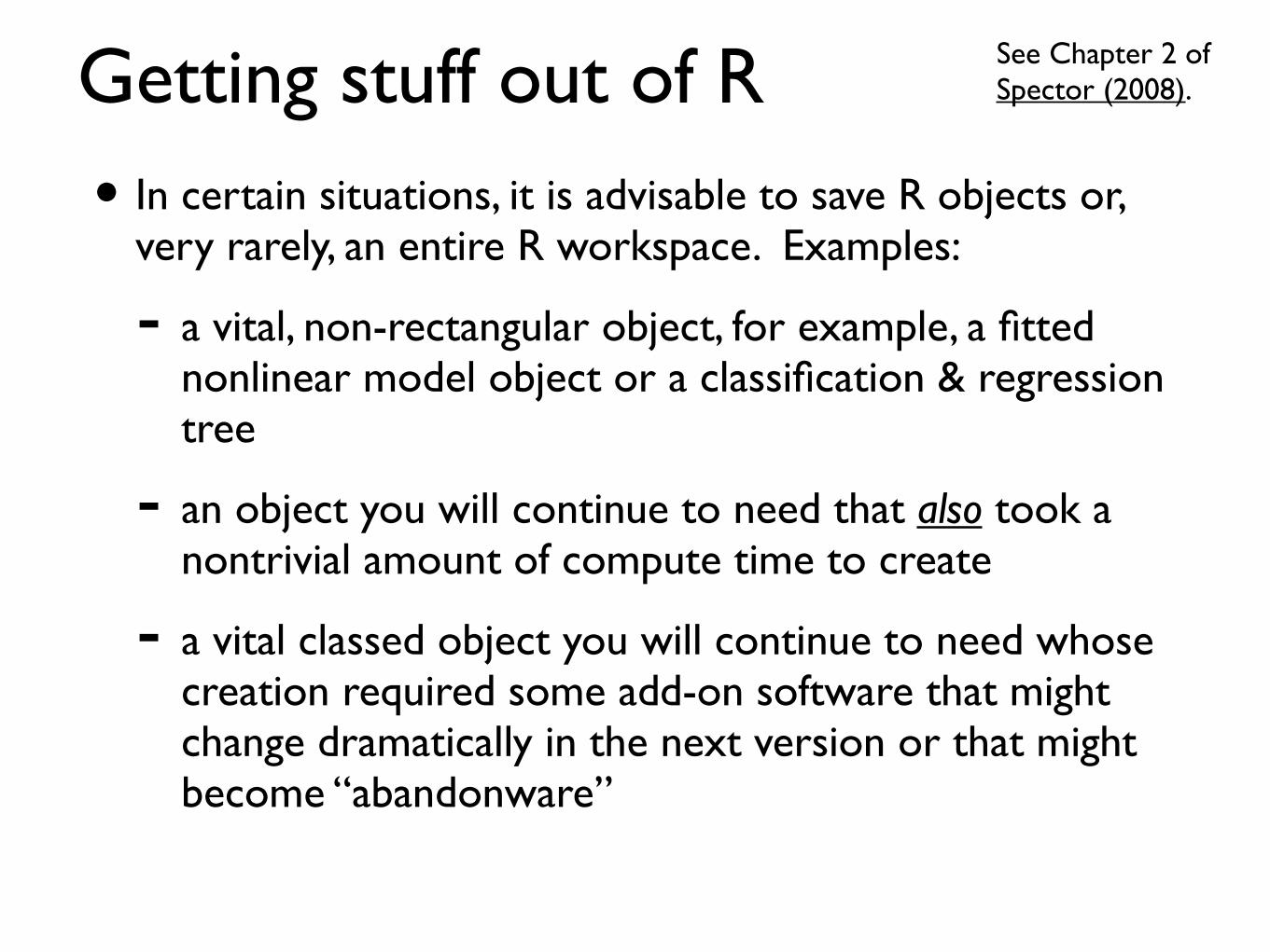
• In certain situations, it is advisable to save R objects or, very rarely, an entire R workspace. Examples:
- a vital, non-rectangular object, for example, a fitted nonlinear model object or a classification & regression tree
- an object you will continue to need that also took a nontrivial amount of compute time to create
- a vital classed object you will continue to need whose creation required some add-on software that might change dramatically in the next version or that might become “abandonware”
See Chapter 2 of Spector (2008).
Getting stuff out of R
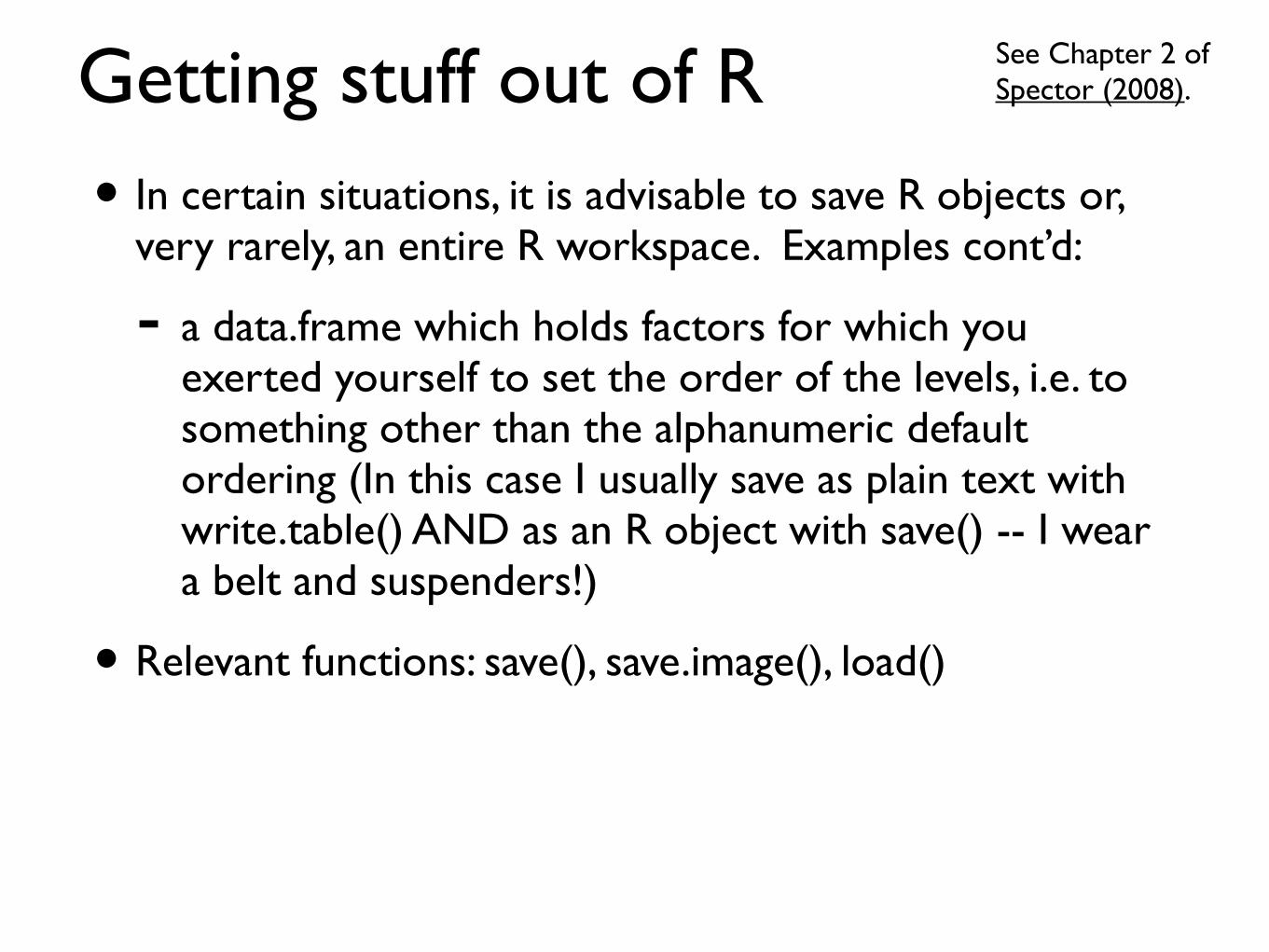
• In certain situations, it is advisable to save R objects or, very rarely, an entire R workspace. Examples cont’d:
- a data.frame which holds factors for which you exerted yourself to set the order of the levels, i.e. to something other than the alphanumeric default ordering (In this case I usually save as plain text with write.table() AND as an R object with save() -- I wear a belt and suspenders!)
• Relevant functions: save(), save.image(), load()
See Chapter 2 of Spector (2008).
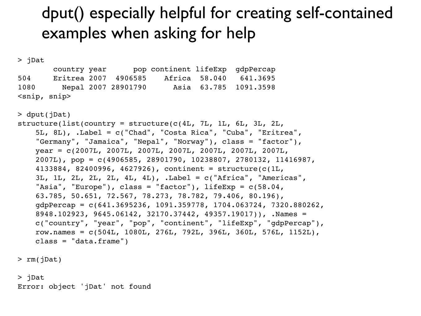
> jDat country year pop continent lifeExp gdpPercap504 Eritrea 2007 4906585 Africa 58.040 641.36951080 Nepal 2007 28901790 Asia 63.785 1091.3598<snip, snip>
> dput(jDat)structure(list(country = structure(c(4L, 7L, 1L, 6L, 3L, 2L, 5L, 8L), .Label = c("Chad", "Costa Rica", "Cuba", "Eritrea", "Germany", "Jamaica", "Nepal", "Norway"), class = "factor"), year = c(2007L, 2007L, 2007L, 2007L, 2007L, 2007L, 2007L, 2007L), pop = c(4906585, 28901790, 10238807, 2780132, 11416987, 4133884, 82400996, 4627926), continent = structure(c(1L, 3L, 1L, 2L, 2L, 2L, 4L, 4L), .Label = c("Africa", "Americas", "Asia", "Europe"), class = "factor"), lifeExp = c(58.04, 63.785, 50.651, 72.567, 78.273, 78.782, 79.406, 80.196), gdpPercap = c(641.3695236, 1091.359778, 1704.063724, 7320.880262, 8948.102923, 9645.06142, 32170.37442, 49357.19017)), .Names = c("country", "year", "pop", "continent", "lifeExp", "gdpPercap"), row.names = c(504L, 1080L, 276L, 792L, 396L, 360L, 576L, 1152L), class = "data.frame")
> rm(jDat)
> jDatError: object 'jDat' not found
dput() especially helpful for creating self-contained examples when asking for help
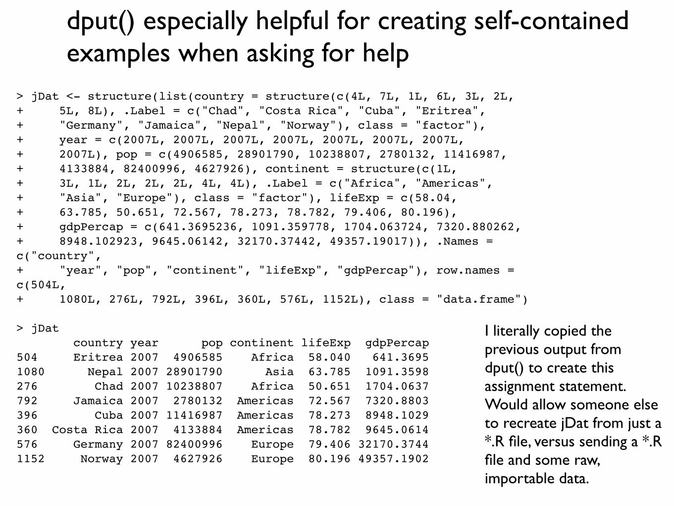
> jDat <- structure(list(country = structure(c(4L, 7L, 1L, 6L, 3L, 2L,+ 5L, 8L), .Label = c("Chad", "Costa Rica", "Cuba", "Eritrea",+ "Germany", "Jamaica", "Nepal", "Norway"), class = "factor"),+ year = c(2007L, 2007L, 2007L, 2007L, 2007L, 2007L, 2007L,+ 2007L), pop = c(4906585, 28901790, 10238807, 2780132, 11416987,+ 4133884, 82400996, 4627926), continent = structure(c(1L,+ 3L, 1L, 2L, 2L, 2L, 4L, 4L), .Label = c("Africa", "Americas",+ "Asia", "Europe"), class = "factor"), lifeExp = c(58.04,+ 63.785, 50.651, 72.567, 78.273, 78.782, 79.406, 80.196),+ gdpPercap = c(641.3695236, 1091.359778, 1704.063724, 7320.880262,+ 8948.102923, 9645.06142, 32170.37442, 49357.19017)), .Names = c("country",+ "year", "pop", "continent", "lifeExp", "gdpPercap"), row.names = c(504L,+ 1080L, 276L, 792L, 396L, 360L, 576L, 1152L), class = "data.frame")
> jDat country year pop continent lifeExp gdpPercap504 Eritrea 2007 4906585 Africa 58.040 641.36951080 Nepal 2007 28901790 Asia 63.785 1091.3598276 Chad 2007 10238807 Africa 50.651 1704.0637792 Jamaica 2007 2780132 Americas 72.567 7320.8803396 Cuba 2007 11416987 Americas 78.273 8948.1029360 Costa Rica 2007 4133884 Americas 78.782 9645.0614576 Germany 2007 82400996 Europe 79.406 32170.37441152 Norway 2007 4627926 Europe 80.196 49357.1902
dput() especially helpful for creating self-contained examples when asking for help
I literally copied the previous output from dput() to create this assignment statement. Would allow someone else to recreate jDat from just a *.R file, versus sending a *.R file and some raw, importable data.
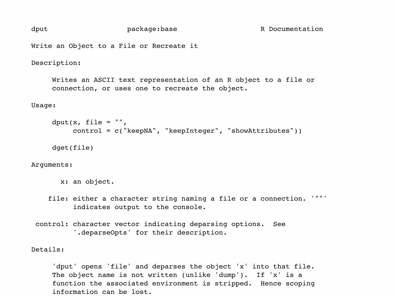
dput package:base R Documentation
Write an Object to a File or Recreate it
Description:
Writes an ASCII text representation of an R object to a file or connection, or uses one to recreate the object.
Usage:
dput(x, file = "", control = c("keepNA", "keepInteger", "showAttributes")) dget(file) Arguments:
x: an object.
file: either a character string naming a file or a connection. '""' indicates output to the console.
control: character vector indicating deparsing options. See '.deparseOpts' for their description.
Details:
'dput' opens 'file' and deparses the object 'x' into that file. The object name is not written (unlike 'dump'). If 'x' is a function the associated environment is stripped. Hence scoping information can be lost.
Deparsing an object is difficult, and not always possible. With the default 'control', 'dput()' attempts to deparse in a way that is readable, but for more complex or unusual objects (see 'dump', not likely to be parsed as identical to the original. Use 'control = "all"' for the most complete deparsing; use 'control = NULL' for the simplest deparsing, not even including attributes.
'dput' will warn if fewer characters were written to a file than expected, which may indicate a full or corrupt file system.
To display saved source rather than deparsing the internal representation include '"useSource"' in 'control'. R currently saves source only for function definitions.
Getting tables out of R
Do not type statistical results into tables in LaTeX or Word or ... (or, at least, that should be the exception, not the rule).
You will make mistakes. You will grow weary of it each time you need to update.
Automate.
Where might you want to put a table computed by R?
In Excel. Easy. Write to a delimited file and import. Done.
In a Word or Pages document, i.e. word processors that have a real concept of a table.
In a Powerpoint or Keynote document. Ditto.
On the web.
In a LaTeX document.
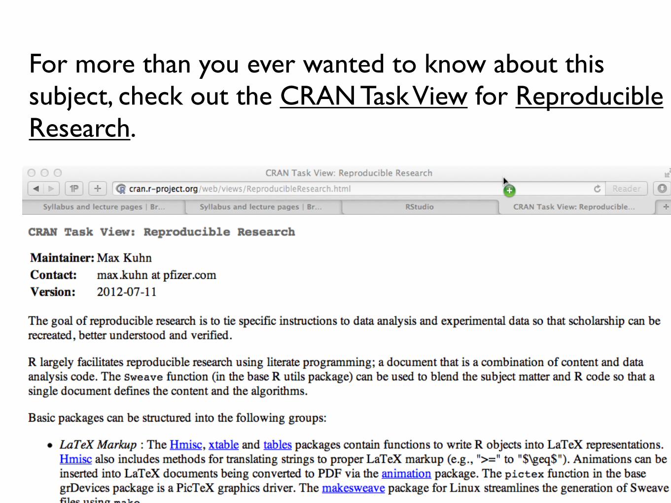
For more than you ever wanted to know about this subject, check out the CRAN Task View for Reproducible Research.
Low-tech solution for Word and Keynote and probably other similar programs ....
Write table to tab-delimited fileopen in text editor, copy contents to clipboardpaste into table-type receptacle in work processing / presentation software OR convert text to table
details will differ but should be workable in many contexts
figure out how to do this with the software you use!
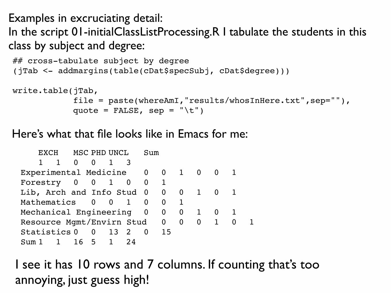
Examples in excruciating detail: In the script 01-initialClassListProcessing.R I tabulate the students in this class by subject and degree:## cross-tabulate subject by degree(jTab <- addmargins(table(cDat$specSubj, cDat$degree)))
write.table(jTab, file = paste(whereAmI,"results/whosInHere.txt",sep=""), quote = FALSE, sep = "\t")
! EXCH! MSC!PHD!UNCL! Sum! 1! 1! 0! 0! 1! 3Experimental Medicine! 0! 0! 1! 0! 0! 1Forestry! 0! 0! 1! 0! 0! 1Lib, Arch and Info Stud! 0! 0! 0! 1! 0! 1Mathematics! 0! 0! 1! 0! 0! 1Mechanical Engineering! 0! 0! 0! 1! 0! 1Resource Mgmt/Envirn Stud! 0! 0! 0! 1! 0! 1Statistics!0! 0! 13! 2! 0! 15Sum!1! 1! 16! 5! 1! 24
Here’s what that file looks like in Emacs for me:
I see it has 10 rows and 7 columns. If counting that’s too annoying, just guess high!
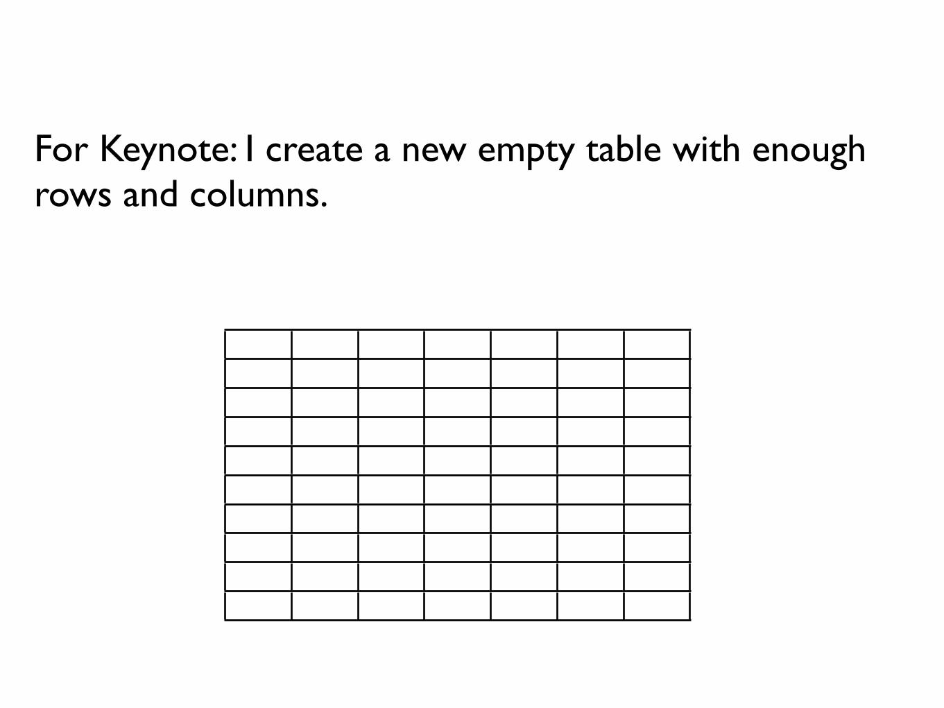
For Keynote: I create a new empty table with enough rows and columns.
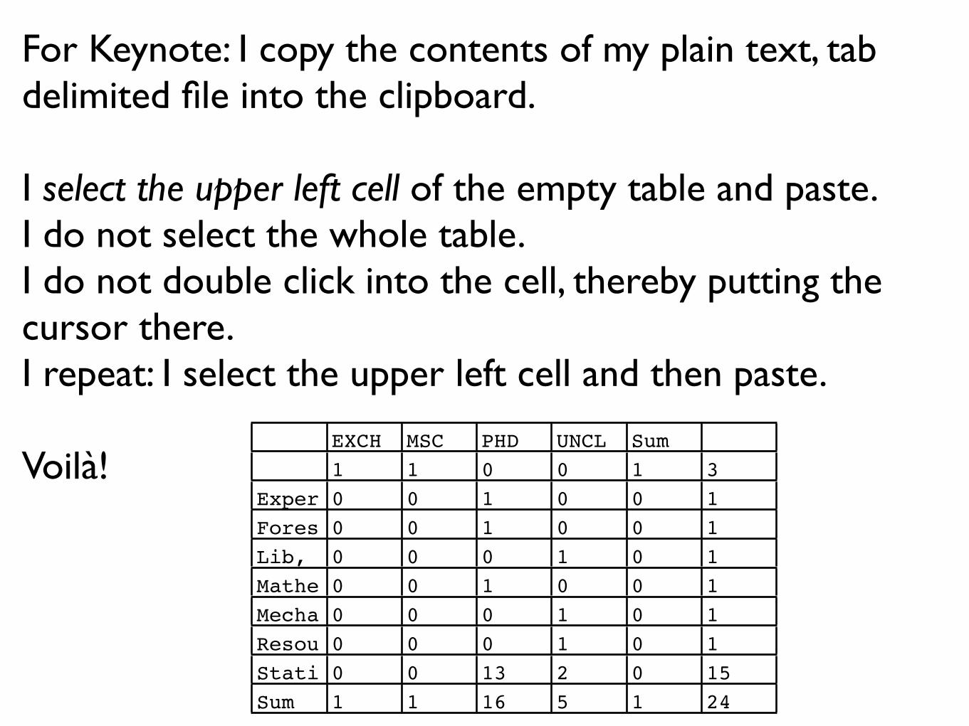
For Keynote: I copy the contents of my plain text, tab delimited file into the clipboard.
I select the upper left cell of the empty table and paste.I do not select the whole table.I do not double click into the cell, thereby putting the cursor there.I repeat: I select the upper left cell and then paste.
Voilà!EXCH MSC PHD UNCL Sum1 1 0 0 1 3
Experimental Medicine
0 0 1 0 0 1Forestry
0 0 1 0 0 1Lib, Arch and Info Stud
0 0 0 1 0 1Mathematics
0 0 1 0 0 1Mechanical Engineering
0 0 0 1 0 1Resource Mgmt/Envir
0 0 0 1 0 1Statistics
0 0 13 2 0 15Sum 1 1 16 5 1 24
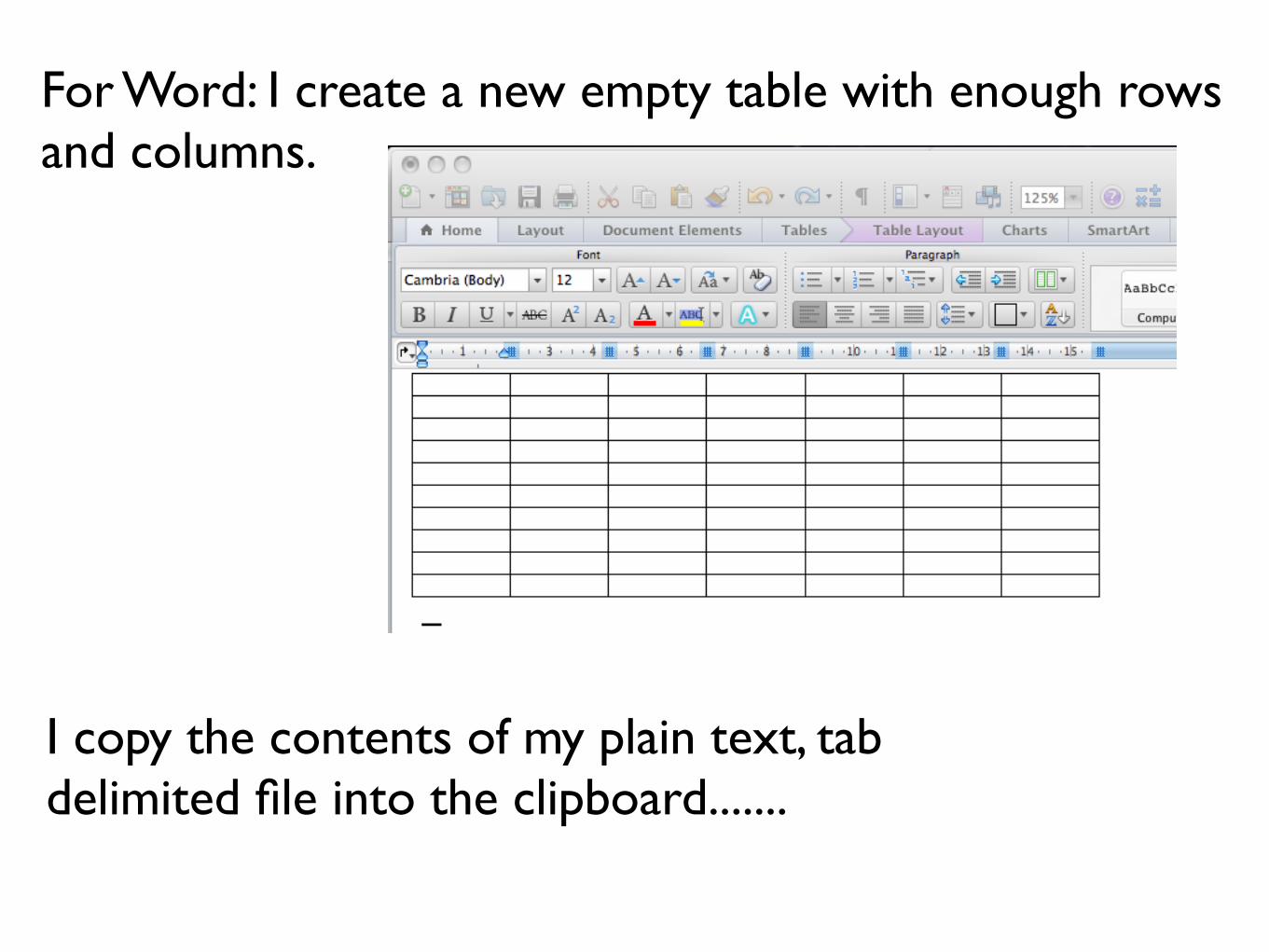
For Word: I create a new empty table with enough rows and columns.
I copy the contents of my plain text, tab delimited file into the clipboard.......
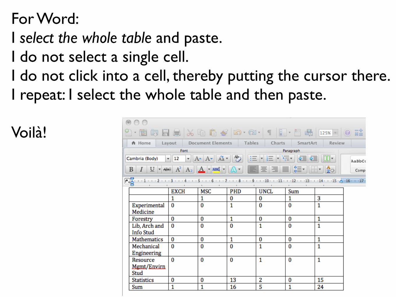
For Word: I select the whole table and paste.I do not select a single cell.I do not click into a cell, thereby putting the cursor there.I repeat: I select the whole table and then paste.
Voilà!
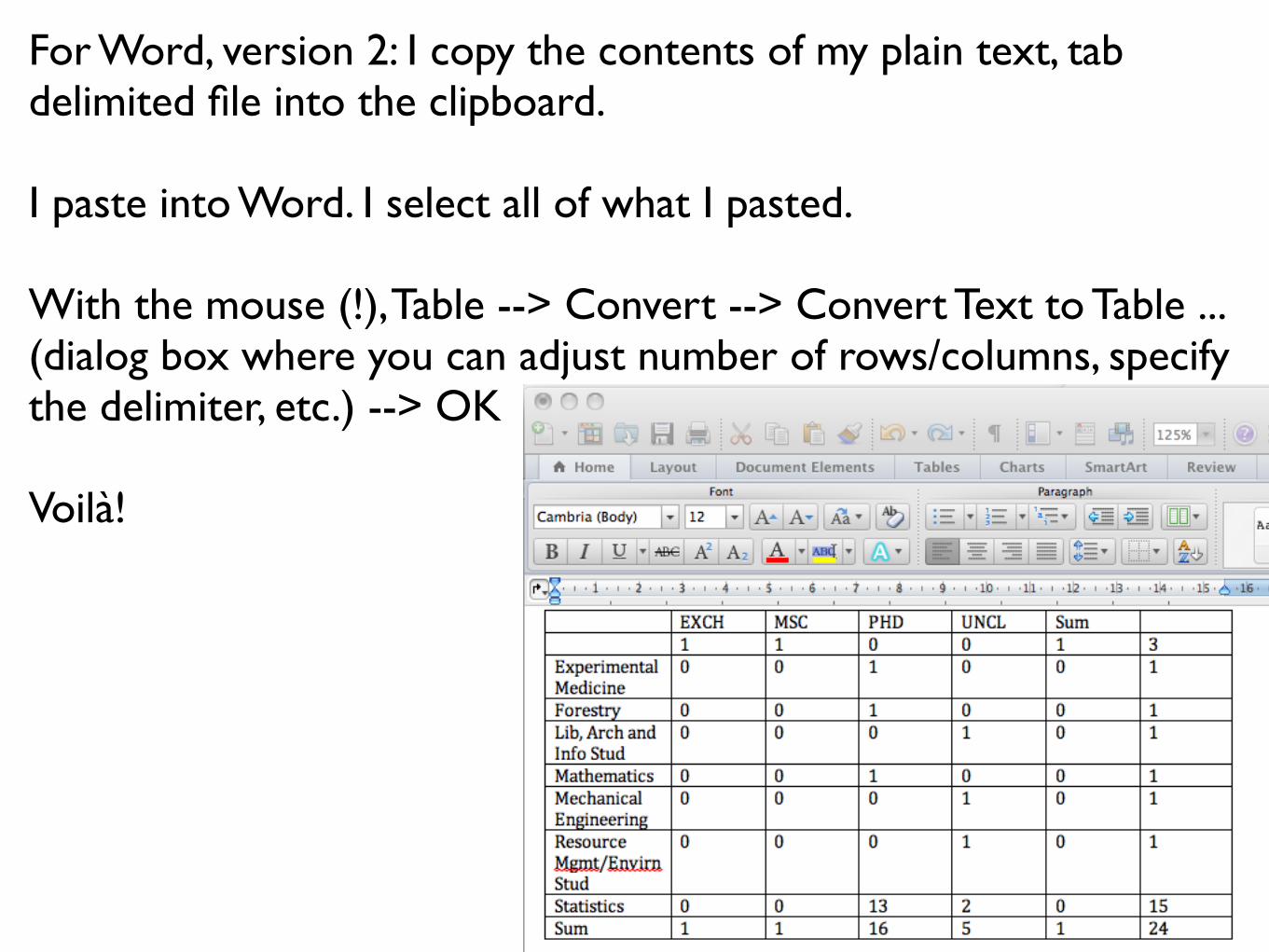
For Word, version 2: I copy the contents of my plain text, tab delimited file into the clipboard.
I paste into Word. I select all of what I pasted.
With the mouse (!), Table --> Convert --> Convert Text to Table ... (dialog box where you can adjust number of rows/columns, specify the delimiter, etc.) --> OK
Voilà!
Getting tables out of RI’ve showed you a low-tech solution for Word and Keynote. Can someone work on PowerPoint?
Good but old thread on how to copy from R to the clipboard; first time I’ve ever seen something work better on Windows! Still relevant? I don’t know know; am on Mac.
The R2wd package looks intriguing but I would worry about fiddliness: “R2wd: Write MS-Word documents from R. This package uses the statconnDCOM server to communicate with MS-Word via the COM interface.”
Use one of these packages to write HTML tables: xtable, Hmisc, R2HTML, hwriter
I use R2HTML .......
How to create an HTML table
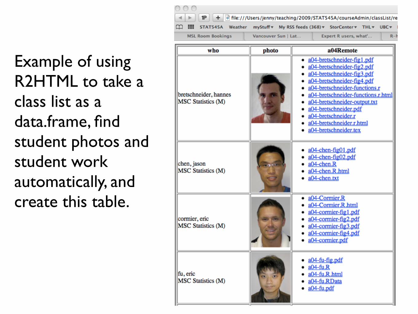
Example of using R2HTML to take a class list as a data.frame, find student photos and student work automatically, and create this table.
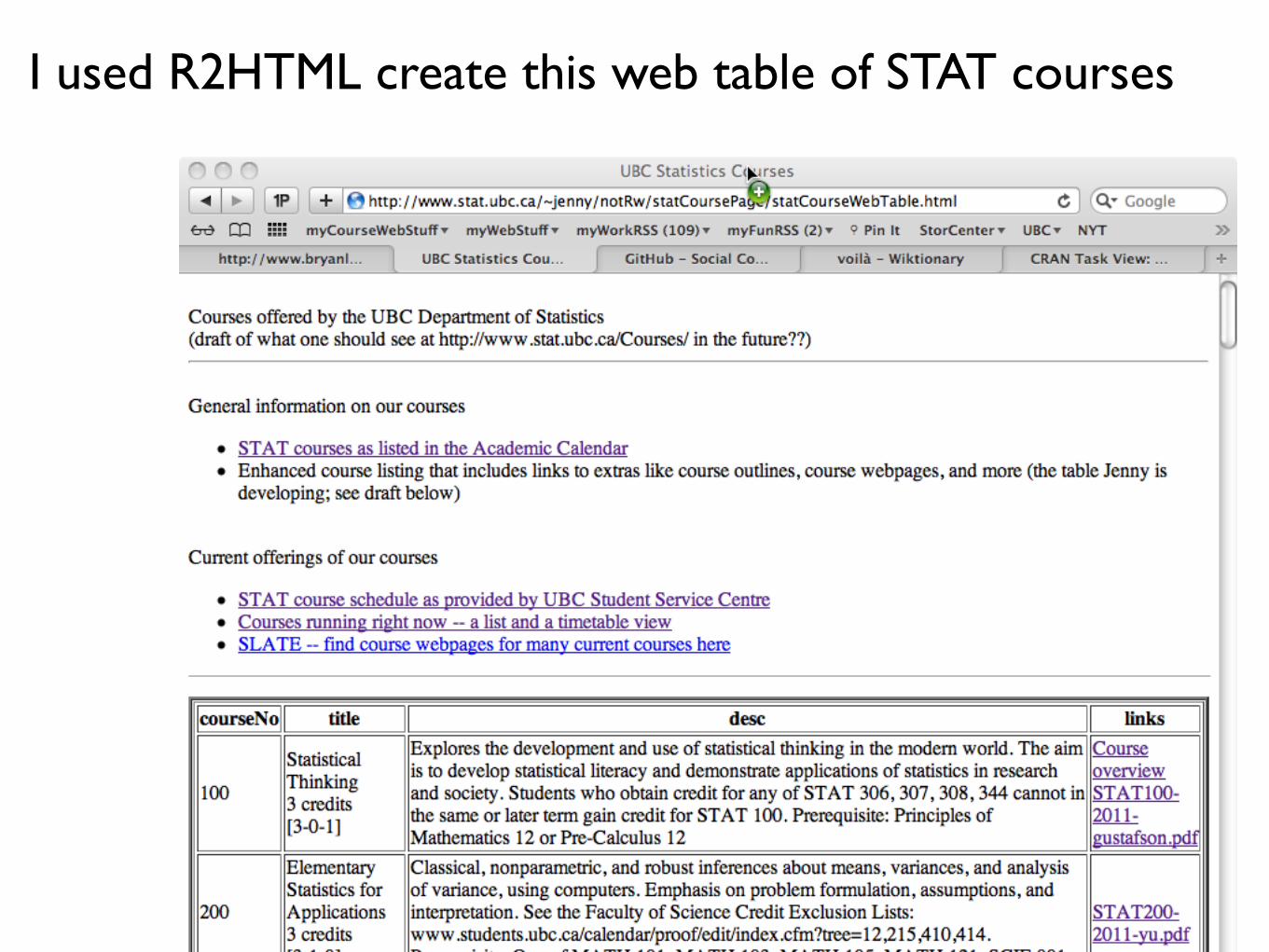
I used R2HTML create this web table of STAT courses
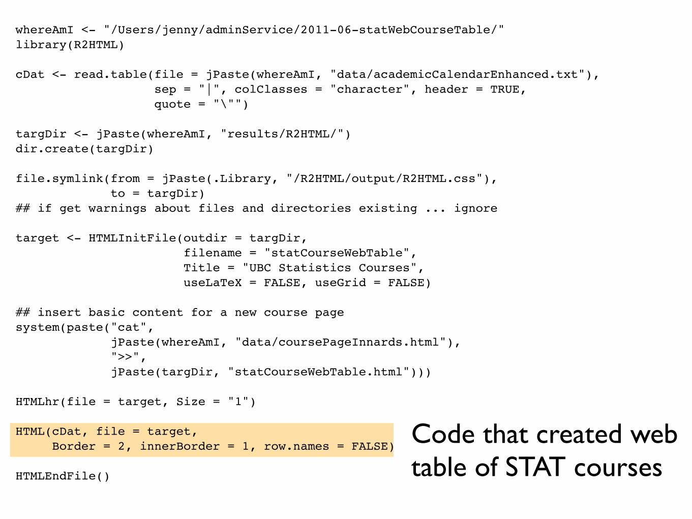
whereAmI <- "/Users/jenny/adminService/2011-06-statWebCourseTable/"library(R2HTML)
cDat <- read.table(file = jPaste(whereAmI, "data/academicCalendarEnhanced.txt"), sep = "|", colClasses = "character", header = TRUE, quote = "\"")
targDir <- jPaste(whereAmI, "results/R2HTML/")dir.create(targDir)
file.symlink(from = jPaste(.Library, "/R2HTML/output/R2HTML.css"), to = targDir)## if get warnings about files and directories existing ... ignore
target <- HTMLInitFile(outdir = targDir, filename = "statCourseWebTable", Title = "UBC Statistics Courses", useLaTeX = FALSE, useGrid = FALSE)
## insert basic content for a new course pagesystem(paste("cat", jPaste(whereAmI, "data/coursePageInnards.html"), ">>", jPaste(targDir, "statCourseWebTable.html")))
HTMLhr(file = target, Size = "1") HTML(cDat, file = target, Border = 2, innerBorder = 1, row.names = FALSE)
HTMLEndFile()
Code that created web table of STAT courses
Use one of these packages to write LaTeX tables: xtable, Hmisc
I don’t use these because I’ve abandoned LaTeX (!), at least for now.
How to create a LaTeX table
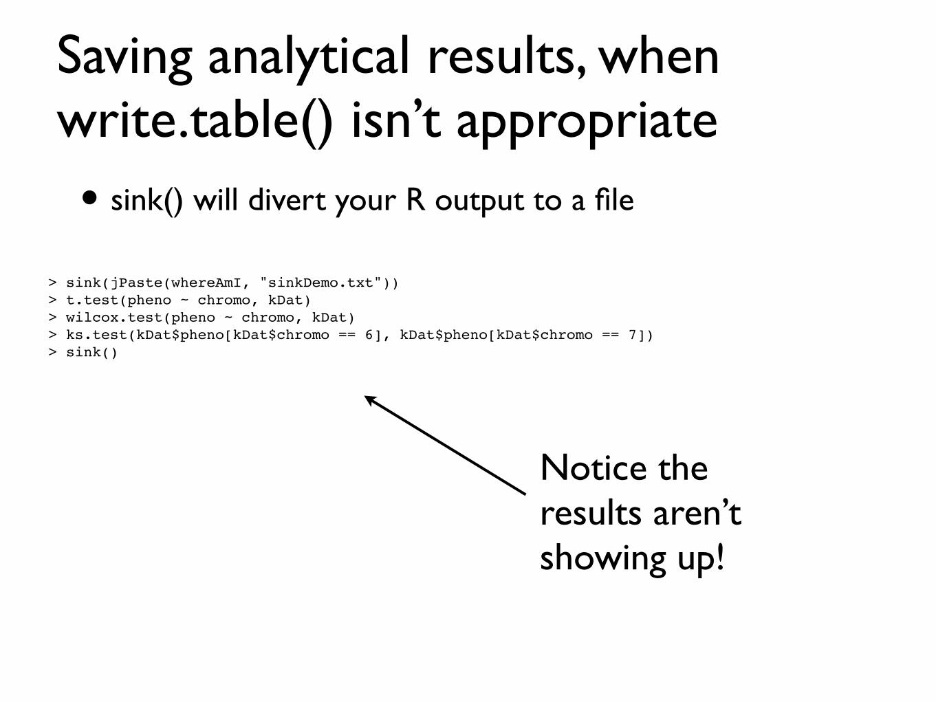
Saving analytical results, when write.table() isn’t appropriate• sink() will divert your R output to a file
> sink(jPaste(whereAmI, "sinkDemo.txt"))> t.test(pheno ~ chromo, kDat)> wilcox.test(pheno ~ chromo, kDat)> ks.test(kDat$pheno[kDat$chromo == 6], kDat$pheno[kDat$chromo == 7])> sink()
Notice the results aren’t showing up!
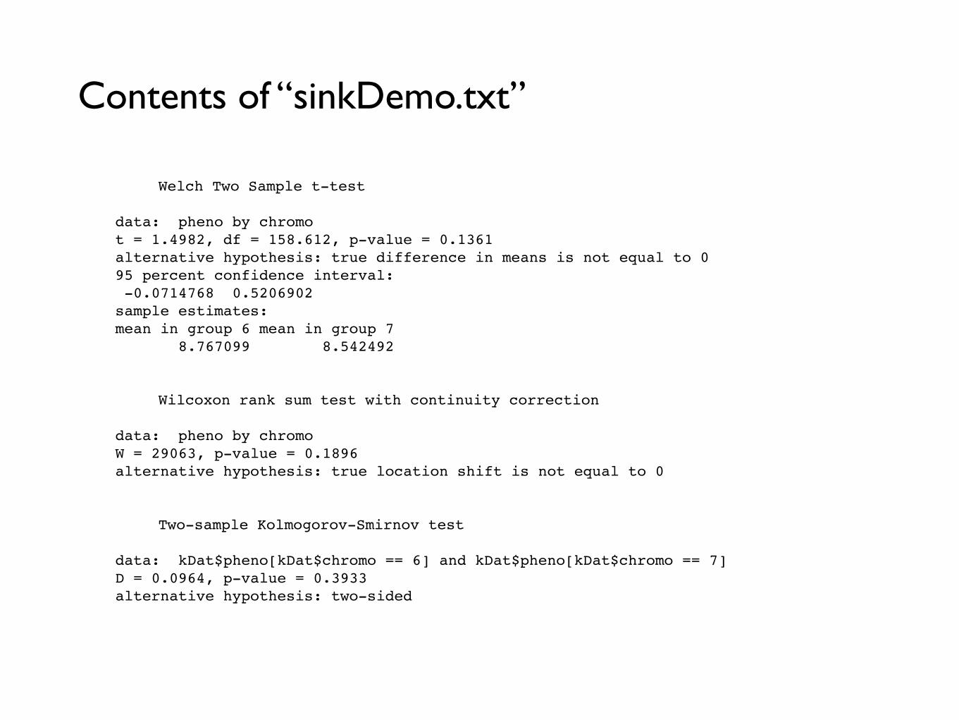
! Welch Two Sample t-test
data: pheno by chromo t = 1.4982, df = 158.612, p-value = 0.1361alternative hypothesis: true difference in means is not equal to 0 95 percent confidence interval: -0.0714768 0.5206902 sample estimates:mean in group 6 mean in group 7 8.767099 8.542492
! Wilcoxon rank sum test with continuity correction
data: pheno by chromo W = 29063, p-value = 0.1896alternative hypothesis: true location shift is not equal to 0
! Two-sample Kolmogorov-Smirnov test
data: kDat$pheno[kDat$chromo == 6] and kDat$pheno[kDat$chromo == 7] D = 0.0964, p-value = 0.3933alternative hypothesis: two-sided
Contents of “sinkDemo.txt”
sink()
• Not a great general purpose, long-run strategy, but useful sometimes
• Must write and debug your code first, then implement sink(), since you “fly blind” while the sink is in place
• Reminds me of the ‘correct’, but annoying way to make PDF files
• Nice when you are ‘source()’ing code and/or running R non-interactively
• Helpful for writing key facts and numbers to file that must be incorporated into written English (vs. a table)