Stat 155, Section 2, Last Time

• Numerical Summaries of Data:– Center: Mean, Medial– Spread: Range, Variance, S.D., IQR

• 5 Number Summary & Outlier Rule

• Transformation & Summaries

• Course Organization & Websitehttp://stat-or.unc.edu/webspace/postscript/marron/Teaching/stor155-2007/Stor155-07Home.html

Reading In Textbook

Approximate Reading for Today’s Material:

Pages 64-83

Approximate Reading for Next Class:

Pages 102-112, 123-127

And now for something completely different

Collect data (into Spreadsheet):

• Years stamped on coins

(chosen denomination)

• Many as person has

• Enter into spreadsheet

• Look at “distribution” using histogram

And now for something completely different

Unfortunately I lost the data…

• Didn’t save file???

• Saved to Strange Location???

• Anyway, I can’t find it…

• So won’t be able to finish this

A Special Request

Professor Marron,

I am having a lot of trouble creating time

plots. Is there any way that you could

walk me through creating one again or

demonstrate on Tuesday? I read over

the notes and the book but that didn't

help. Thanks!

Exploratory Data Analysis 3

“Time Plots”, i.e. “Time Series:

Idea: when time structure is important,

plot variable as a function of time:

variable

time

Often useful to “connect the dots”

Airline Passengers Example

A look under the hoodhttp://stat-or.unc.edu/webspace/postscript/marron/Teaching/stor155-2007/Stor155Eg5Done.xls

• Use Chart Wizard

• Chart Type: Line (or could do XY)

• Use subtype for points & lines

• Use menu for first log10

• Although could just type it in

• Drag down to repeat for whole column

Modelling Distributions

Text: Section 1.3

Idea: Approximate histograms by:

an “idealized curve”

i.e. a “density curve”

that represents the underlying population

Idealized Curve Example

Recall Hidalgo Stamps Data,

Shifting Bin Movie (made # modes change):http://stat-or.unc.edu/webspace/postscript/marron/Teaching/stor155-2007/StampsHistLoc.mpg

Add idealized curve:http://stat-or.unc.edu/webspace/postscript/marron/Teaching/stor155-2007/StampsHistLocKDE.mpg

Note: “population curve” shows why

histogram modes appear and disappear

Interpretation of Density

Areas under density curve,

give “relative frequency”

Proportion of data between =

= Area under =

ba &

b

adxxf )()(xf

a b

Interpretation of Density

Note: Total Area under density = 1

(since relative freq. of everything is 1)

HW: 1.80 (a: l = w = 1 b: 0.25 c: 0.5),

1.81, 1.83

• Work with pencil and paper, not EXCEL

Most Useful Density

“Normal Curve” = “Gaussian Density”

• Shape: “like a mound”

• E.g. of “sand dumped from a truck”

• Older, worse, description: “bell shaped”

Normal Density Example

Winter Daily Maximum Temperatures in

Melbourne, Australiahttp://stat-or.unc.edu/webspace/postscript/marron/Teaching/stor155-2007/Stor155Eg8Done.xls

Notes:

• Top Histogram is “mound shaped”

• Plus “small scale random variation”

• So model with “Normal Density”?

Normal Density Curves

Note: there is a family of normal curves,

indexed by:

i. “Center”, i.e. Mean =

ii. “Spread”, i.e. Stand. Deviation =

Terminology: & are called “parameters”

Greek “mu” ~ m Greek “sigma” ~ s

Family of Normal Curves

Think about:

• “Shifts” (pans) indexed by

• “Scales” (zooms) indexed by

Nice interactive graphical example:

http://www.stat.sc.edu/~west/applets/normaldemo1.html

(note area under curve is always 1)

Normal Curve Mathematics

The “normal density curve” is:

usual “function” of

circle constant = 3.14…

natural number =

2.7…

,2

21

21

)(

x

exf

x

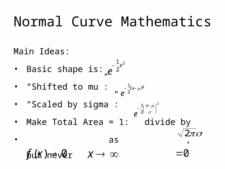
Normal Curve Mathematics

Main Ideas:

• Basic shape is:

• “Shifted to mu”:

• “Scaled by sigma”:

• Make Total Area = 1: divide by

• as , but never

2

21x

e

2

0

221 x

e2

21

x

e

0)( xf x

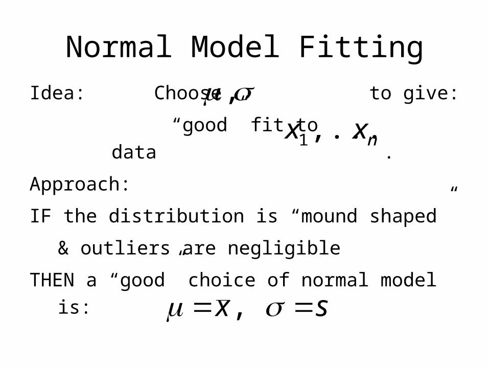
Normal Model Fitting

Idea: Choose to give:

“good” fit to data .

Approach:

IF the distribution is “mound shaped”

& outliers are negligible

THEN a “good” choice of normal model is:

nxx ,...,1

,

sx ,

Normal Fitting Example

Revisit Melbourne Daily Max Tempshttp://stat-or.unc.edu/webspace/postscript/marron/Teaching/stor155-2007/Stor155Eg8Done.xls

• Fit curve, using

• “Visually good” approximation

sx ,

Normal Fitting Example

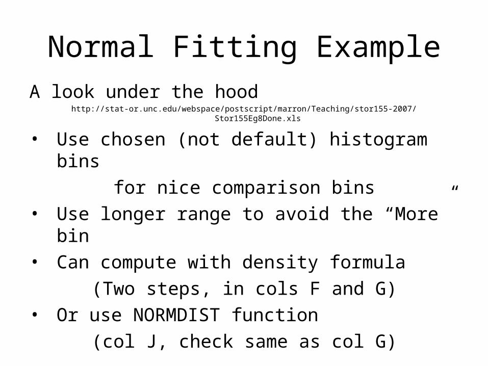
A look under the hoodhttp://stat-or.unc.edu/webspace/postscript/marron/Teaching/stor155-2007/Stor155Eg8Done.xls

• Use chosen (not default) histogram bins

for nice comparison bins

• Use longer range to avoid the “More” bin

• Can compute with density formula

(Two steps, in cols F and G)

• Or use NORMDIST function

(col J, check same as col G)

Normal Curve HW

C5: A study of distance runners found a

mean weight of 63.1 kg, with a standard

deviation of 4.8 kg. Assuming that the

distribution of weights is normal, use

EXCEL to draw the density curve of the

weight distribution.