Stat 112: Lecture 10 Notes

• Fitting Curvilinear Relationships– Polynomial Regression (Ch. 5.2.1)– Transformations (Ch. 5.2.2-5.2.4)

• Schedule: – Homework 3 due on Thursday.– Quiz 2 next

Curvilinear Relationship

• Reconsider the simple regression problem of estimating the conditional mean of y given x,

• For many problems, is not linear. • Linear regression model makes restrictive

assumption that increase in mean of y|x for a one unit increase in x equals

• Curvilinear relationship: is a curve, not a straight line; increase in mean of y|x is not the same for all x.

( | )E y x

( | )E y x

1( | )E y x

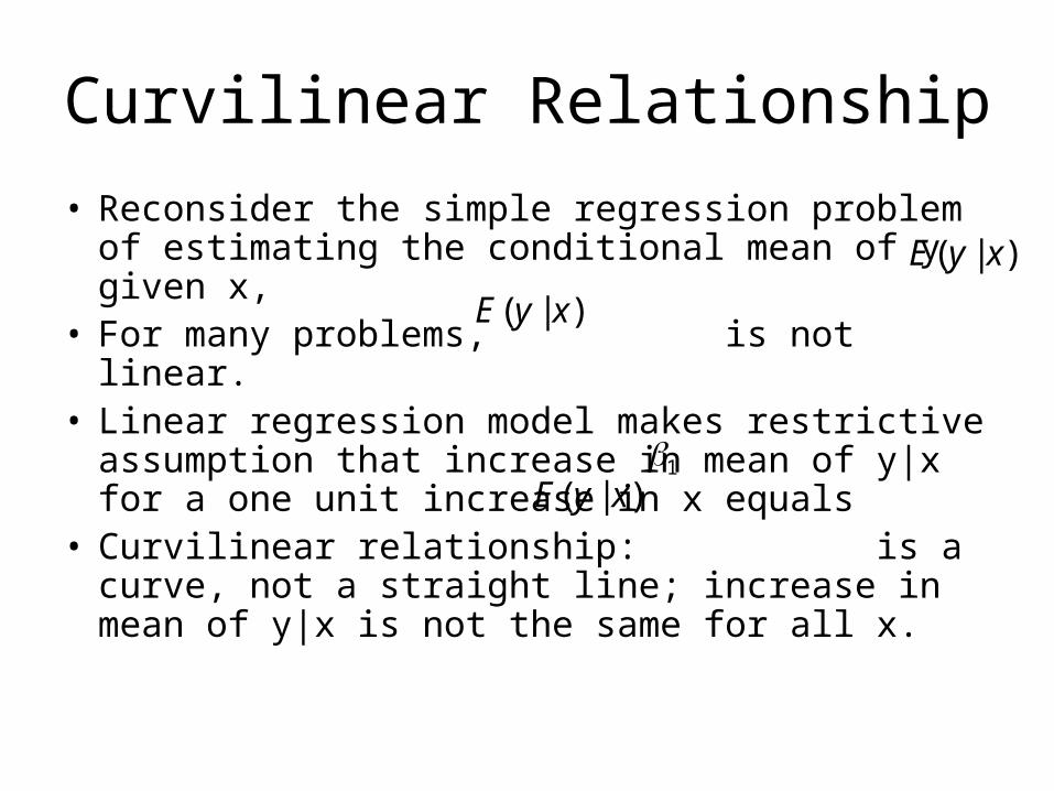
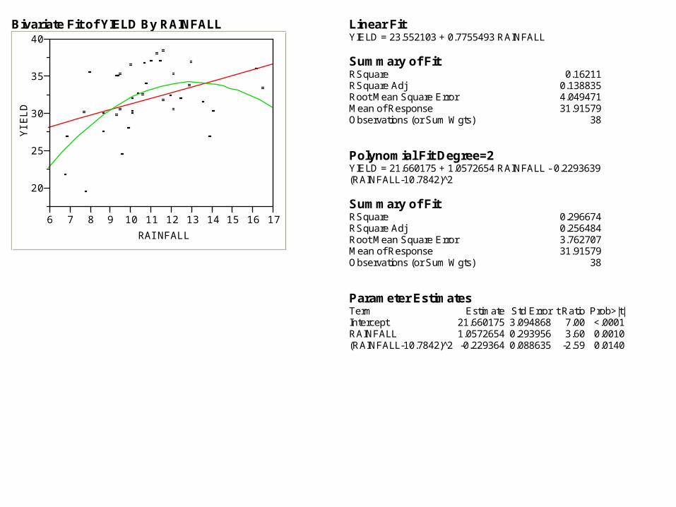
Example 1: How does rainfall affect yield?

• Data on average corn yield and rainfall in six U.S. states (1890-1927), cornyield.JMP

20

25

30

35

40

YIE

LD

6 7 8 9 10 11 12 13 14 15 16 17

RAINFALL

Bivariate Fit of YIELD By RAINFALL

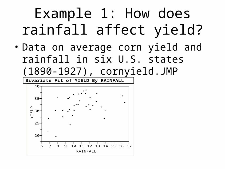
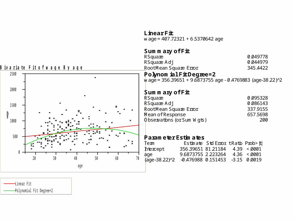
Example 2: How do people’s incomes change as they age

• Weekly wages and age of 200 randomly chosen males between ages 18 and 70 from the 1998 March Current Population SurveyBivariate Fit of wage By age

0

500

1000

1500

2000

2500

wa

ge

20 30 40 50 60 70

age

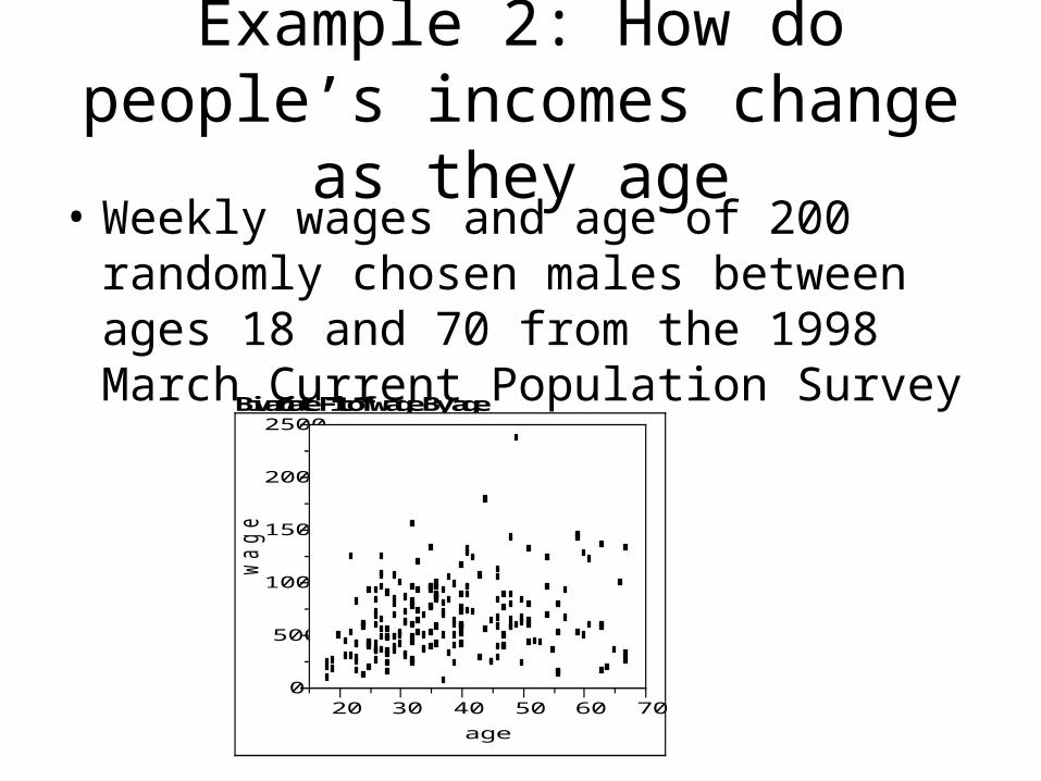
Example 3: Display.JMP

• A large chain of liquor stores would like to know how much display space in its stores to devote to a new wine. It collects sales and display space data from 47 of its stores.Bivariate Fit of Sales By DisplayFeet

0

50

100

150

200

250

300

350

400

450

Sa

les

0 1 2 3 4 5 6 7 8

DisplayFeet

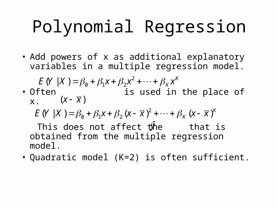
Polynomial Regression

• Add powers of x as additional explanatory variables in a multiple regression model.

• Often is used in the place of x.

This does not affect the that is obtained from the multiple regression model.

• Quadratic model (K=2) is often sufficient.

20 1 2( | ) K

KE Y X x x x

( )x x2

0 1 2( | ) ( ) ( )KKE Y X x x x x x y

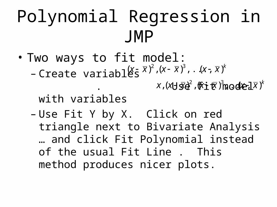
Polynomial Regression in JMP

• Two ways to fit model:– Create variables . Use

fit model with variables – Use Fit Y by X. Click on red triangle next to

Bivariate Analysis … and click Fit Polynomial instead of the usual Fit Line . This method produces nicer plots.

kxxxxxx )(,...,)(,)( 32 kxxxxxxx )(,...,)(,)(, 32

Bivariate Fit of YIELD By RAINFALL

20

25

30

35

40

YIE

LD

6 7 8 9 10 11 12 13 14 15 16 17

RAINFALL

Linear Fit YIELD = 23.552103 + 0.7755493 RAINFALL Summary of Fit RSquare 0.16211 RSquare Adj 0.138835 Root Mean Square Error 4.049471 Mean of Response 31.91579 Observations (or Sum Wgts) 38 Polynomial Fit Degree=2 YIELD = 21.660175 + 1.0572654 RAINFALL - 0.2293639 (RAINFALL-10.7842)^2 Summary of Fit RSquare 0.296674 RSquare Adj 0.256484 Root Mean Square Error 3.762707 Mean of Response 31.91579 Observations (or Sum Wgts) 38 Parameter Estimates Term Estimate Std Error t Ratio Prob>|t| Intercept 21.660175 3.094868 7.00 <.0001 RAINFALL 1.0572654 0.293956 3.60 0.0010 (RAINFALL-10.7842)^2 -0.229364 0.088635 -2.59 0.0140

B i v a r i a t e F i t o f w a g e B y a g e

0

50 0

10 00

15 00

20 00

25 00

wage

2 0 30 40 50 60 70

ag e

L in ea r Fit

Po ly n omia l Fit De gre e=2

Linear Fit wage = 407.72321 + 6.5370642 age Summary of Fit RSquare 0.049778 RSquare Adj 0.044979 Root Mean Square Error 345.4422 Polynomial Fit Degree=2 wage = 356.39651 + 9.6873755 age - 0.4769883 (age-38.22)^2 Summary of Fit RSquare 0.095328 RSquare Adj 0.086143 Root Mean Square Error 337.9155 Mean of Response 657.5698 Observations (or Sum Wgts) 200 Parameter Estimates Term Estimate Std Error t Ratio Prob>|t| Intercept 356.39651 81.21184 4.39 <.0001 age 9.6873755 2.223264 4.36 <.0001 (age-38.22)^2 -0.476988 0.151453 -3.15 0.0019

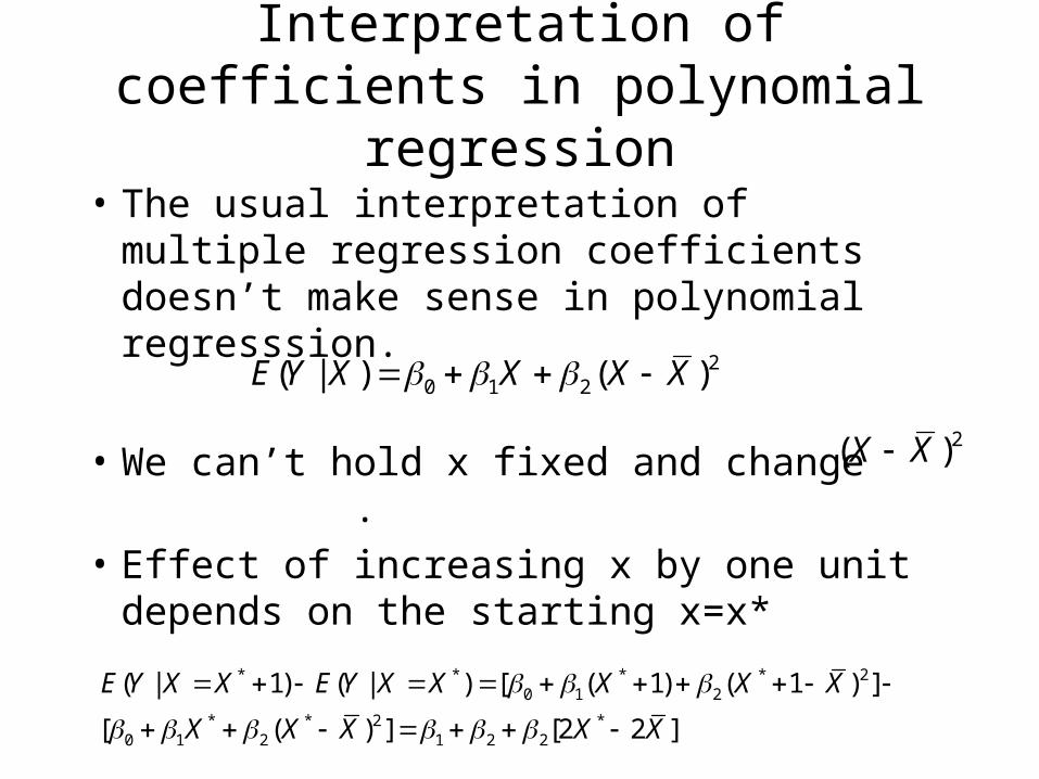
Interpretation of coefficients in polynomial regression

• The usual interpretation of multiple regression coefficients doesn’t make sense in polynomial regresssion.

• We can’t hold x fixed and change .

• Effect of increasing x by one unit depends on the starting x=x*

20 1 2( | ) ( )E Y X X X X

2( )X X

* * * * 20 1 2

* * 2 *0 1 2 1 2 2

( | 1) ( | ) [ ( 1) ( 1 ) ]

[ ( ) ] [2 2 ]

E Y X X E Y X X X X X

X X X X X

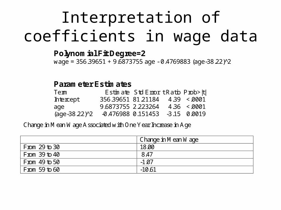
Interpretation of coefficients in wage data

Polynomial Fit Degree=2 wage = 356.39651 + 9.6873755 age - 0.4769883 (age-38.22)^2 Parameter Estimates Term Estimate Std Error t Ratio Prob>|t| Intercept 356.39651 81.21184 4.39 <.0001 age 9.6873755 2.223264 4.36 <.0001 (age-38.22)^2 -0.476988 0.151453 -3.15 0.0019

Change in Mean Wage Associated with One Year Increase in Age Change in Mean Wage From 29 to 30 18.00 From 39 to 40 8.47 From 49 to 50 -1.07 From 59 to 60 -10.61

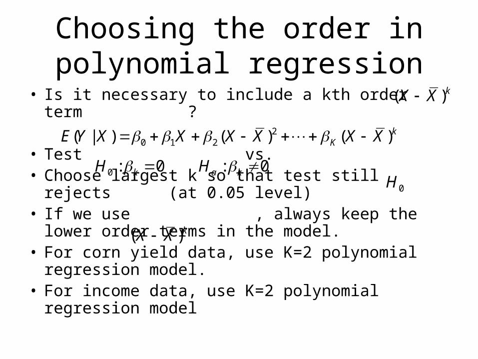
Choosing the order in polynomial regression

• Is it necessary to include a kth order term ?

• Test vs.• Choose largest k so that test still rejects (at 0.05

level)• If we use , always keep the lower order

terms in the model. • For corn yield data, use K=2 polynomial regression

model. • For income data, use K=2 polynomial regression

model

( )kX X

20 1 2( | ) ( ) ( )kKE Y X X X X X X

0:0 kH 0: kaH

( )kX X

0H

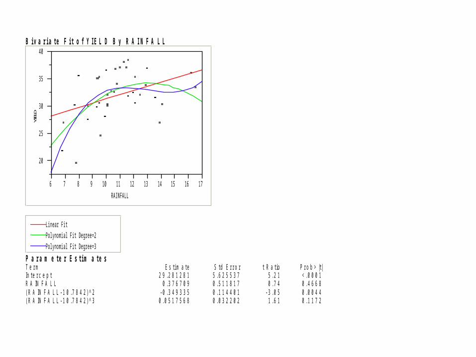
B i v a r i a t e F i t o f Y I E L D B y R A I N F A L L

20

25

30

35

40

YIELD

6 7 8 9 10 11 12 13 14 15 16 17

RAINFALL

L inea r Fit

Po ly nomia l Fit Degree=2

Po ly nomia l Fit Degree=3 P a r a m e t e r E s t i m a t e s T e r m E s t i m a t e S t d E r r o r t R a t i o P r o b > | t | In t e r c e p t 2 9 . 2 8 1 2 8 1 5 . 6 2 5 5 3 7 5 . 2 1 < . 0 0 0 1 R A IN F A L L 0 . 3 7 6 7 0 9 0 . 5 1 1 8 1 7 0 . 7 4 0 . 4 6 6 8 ( R A IN F A L L - 1 0 . 7 8 4 2 ) ^ 2 - 0 . 3 4 9 3 3 5 0 . 1 1 4 4 0 1 - 3 . 0 5 0 . 0 0 4 4 ( R A IN F A L L - 1 0 . 7 8 4 2 ) ^ 3 0 . 0 5 1 7 5 6 8 0 . 0 3 2 2 0 2 1 . 6 1 0 . 1 1 7 2

Transformations

• Curvilinear relationship: E(Y|X) is not a straight line.

• Another approach to fitting curvilinear relationships is to transform Y or x.

• Transformations: Perhaps E(f(Y)|g(X)) is a straight line, where f(Y) and g(X) are transformations of Y and X, and a simple linear regression model holds for the response variable f(Y) and explanatory variable g(X).

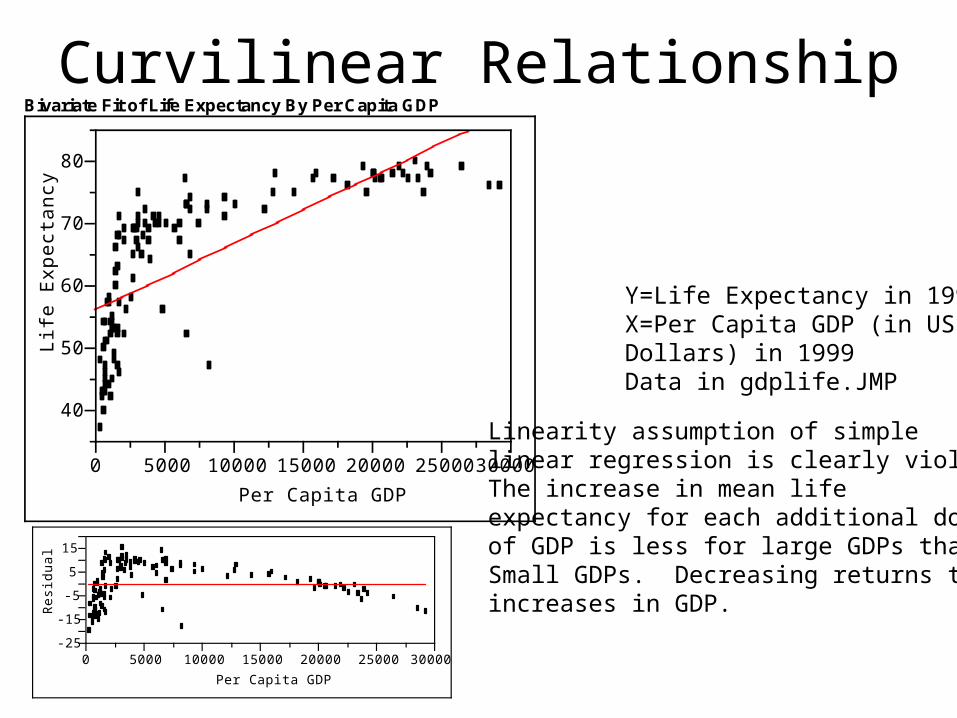
Curvilinear RelationshipBivariate Fit of Life Expectancy By Per Capita GDP

40

50

60

70

80

Life

Exp

ecta

ncy

0 5000 10000 15000 20000 25000 30000

Per Capita GDP

-25

-15

-5

5

15

Res

idua

l

0 5000 10000 15000 20000 25000 30000

Per Capita GDP

Y=Life Expectancy in 1999X=Per Capita GDP (in US Dollars) in 1999Data in gdplife.JMP

Linearity assumption of simplelinear regression is clearly violated.The increase in mean life expectancy for each additional dollarof GDP is less for large GDPs thanSmall GDPs. Decreasing returns toincreases in GDP.

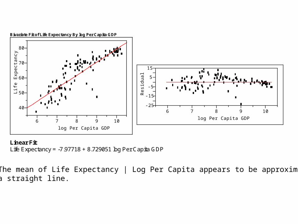
Bivariate Fit of Life Expectancy By log Per Capita GDP

40

50

60

70

80

Life

Exp

ecta

ncy

6 7 8 9 10

log Per Capita GDP

Linear Fit Life Expectancy = -7.97718 + 8.729051 log Per Capita GDP

-25

-15

-5

5

15

Res

idua

l

6 7 8 9 10

log Per Capita GDP

The mean of Life Expectancy | Log Per Capita appears to be approximatelya straight line.

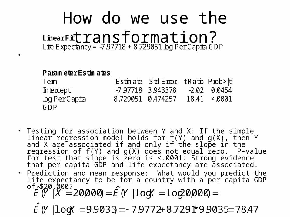
How do we use the transformation?

•

• Testing for association between Y and X: If the simple linear regression model holds for f(Y) and g(X), then Y and X are associated if and only if the slope in the regression of f(Y) and g(X) does not equal zero. P-value for test that slope is zero is <.0001: Strong evidence that per capita GDP and life expectancy are associated.

• Prediction and mean response: What would you predict the life expectancy to be for a country with a per capita GDP of $20,000?

Linear Fit Life Expectancy = -7.97718 + 8.729051 log Per Capita GDP Parameter Estimates Term Estimate Std Error t Ratio Prob>|t| Intercept -7.97718 3.943378 -2.02 0.0454 log Per Capita GDP

8.729051 0.474257 18.41 <.0001

47.789035.9*7291.89772.7)9035.9log|(ˆ

)000,20loglog|(ˆ)000,20|(ˆ

XYE

XYEXYE

How do we choose a transformation?

• Tukey’s Bulging Rule.

• See Handout.

• Match curvature in data to the shape of one of the curves drawn in the four quadrants of the figure in the handout. Then use the associated transformations, selecting one for either X, Y or both.

Transformations in JMP1. Use Tukey’s Bulging rule (see handout) to determine

transformations which might help. 2. After Fit Y by X, click red triangle next to Bivariate Fit and click Fit

Special. Experiment with transformations suggested by Tukey’s Bulging rule.

3. Make residual plots of the residuals for transformed model vs. the original X by clicking red triangle next to Transformed Fit to … and clicking plot residuals. Choose transformations which make the residual plot have no pattern in the mean of the residuals vs. X.

4. Compare different transformations by looking for transformation with smallest root mean square error on original y-scale. If using a transformation that involves transforming y, look at root mean square error for fit measured on original scale.

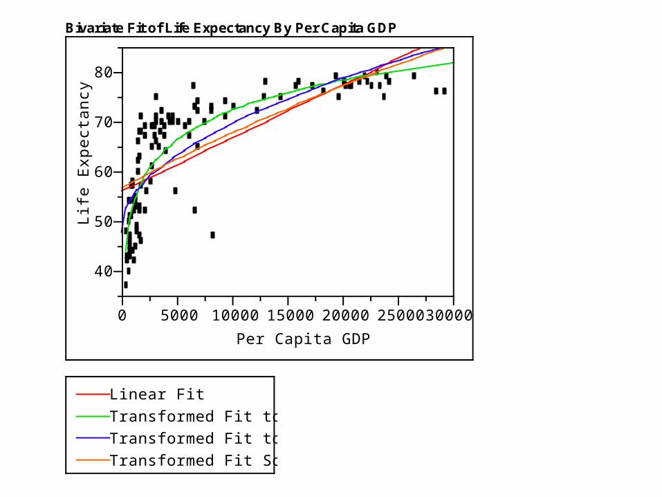
Bivariate Fit of Life Expectancy By Per Capita GDP

40

50

60

70

80Li

fe E

xpec

tanc

y

0 5000 10000 15000 20000 25000 30000

Per Capita GDP

Linear Fit

Transformed Fit to Log

Transformed Fit to Sqrt

Transformed Fit Square

`

•

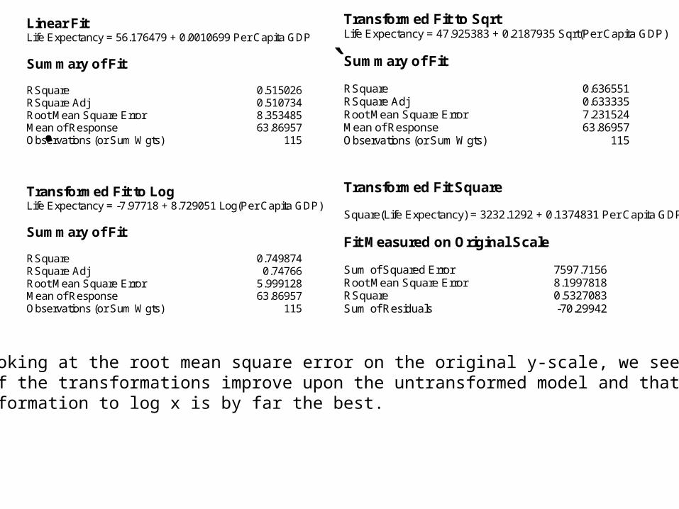
Linear Fit Life Expectancy = 56.176479 + 0.0010699 Per Capita GDP Summary of Fit RSquare 0.515026 RSquare Adj 0.510734 Root Mean Square Error 8.353485 Mean of Response 63.86957 Observations (or Sum Wgts) 115 Transformed Fit to Log Life Expectancy = -7.97718 + 8.729051 Log(Per Capita GDP) Summary of Fit RSquare 0.749874 RSquare Adj 0.74766 Root Mean Square Error 5.999128 Mean of Response 63.86957 Observations (or Sum Wgts) 115

Transformed Fit to Sqrt Life Expectancy = 47.925383 + 0.2187935 Sqrt(Per Capita GDP) Summary of Fit RSquare 0.636551 RSquare Adj 0.633335 Root Mean Square Error 7.231524 Mean of Response 63.86957 Observations (or Sum Wgts) 115 Transformed Fit Square Square(Life Expectancy) = 3232.1292 + 0.1374831 Per Capita GDP Fit Measured on Original Scale Sum of Squared Error 7597.7156 Root Mean Square Error 8.1997818 RSquare 0.5327083 Sum of Residuals -70.29942

By looking at the root mean square error on the original y-scale, we see thatall of the transformations improve upon the untransformed model and that the transformation to log x is by far the best.

Linear Fit

-25

-15

-5

5

15

Res

idua

l

0 5000 10000 15000 20000 25000 30000

Per Capita GDP

Transformation to Log X

-25

-15

-5

5

15

Res

idua

l

0 5000 10000 15000 20000 25000 30000

Per Capita GDP

Transformation to X

-25

-15

-5

5

15

Res

idua

l

0 5000 10000 15000 20000 25000 30000

Per Capita GDP

Transformation to 2Y

-25

-15

-5

5

15

Res

idua

l

0 5000 10000 15000 20000 25000 30000

Per Capita GDP

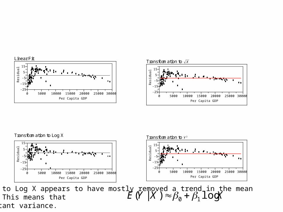
The transformation to Log X appears to have mostly removed a trend in the meanof the residuals. This means that . There is still a problem of nonconstant variance.

XXYE log)|( 10

Comparing models for curvilinear relationships

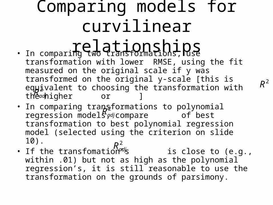
• In comparing two transformations, use transformation with lower RMSE, using the fit measured on the original scale if y was transformed on the original y-scale [this is equivalent to choosing the transformation with the higher or ]

• In comparing transformations to polynomial regression models, compare of best transformation to best polynomial regression model (selected using the criterion on slide 10).

• If the transfomation’s is close to (e.g., within .01) but not as high as the polynomial regression’s, it is still reasonable to use the transformation on the grounds of parsimony.

2adjR

2R2adjR

2adjR

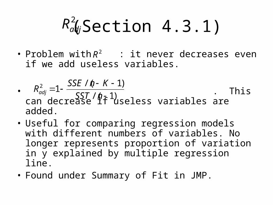
(Section 4.3.1)

• Problem with : it never decreases even if we add useless variables.

• . This can decrease if useless variables are added.

• Useful for comparing regression models with different numbers of variables. No longer represents proportion of variation in y explained by multiple regression line.

• Found under Summary of Fit in JMP.

2adjR

2R

)1/(

)1/(12

nSST

KnSSERadj

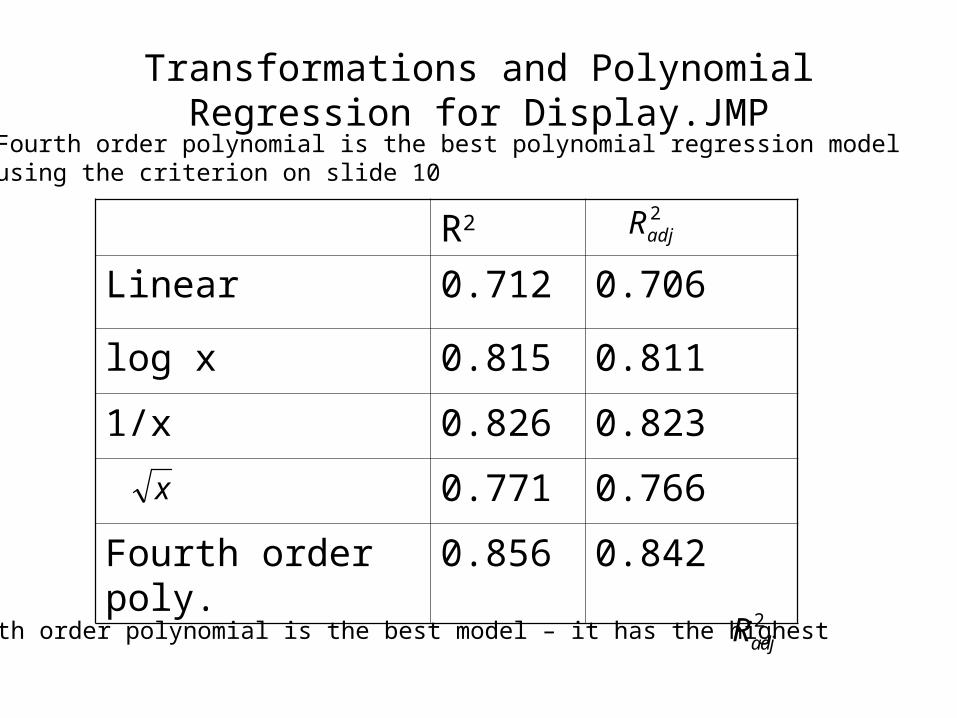
Transformations and Polynomial Regression for Display.JMP

R2

Linear 0.712 0.706

log x 0.815 0.811

1/x 0.826 0.823

0.771 0.766

Fourth order poly. 0.856 0.842

2adjR

x

Fourth order polynomial is the best polynomial regression model using the criterion on slide 10

Fourth order polynomial is the best model – it has the highest 2adjR

Summary

• Two methods for fitting regression models for curvilinear relationships: – Polynomial Regression– Transformations