Embed Size (px)
Citation preview
An observational introduction to star formation Rahila Amlany (209334137) Phys 5290-‐ Extragalactic astronomy Presentation II
1
Table of content page
9.1 Giant Molecular Clouds 2
9.1.1 Observed properties 2
9.1.2 Dynamical state 3
• GMCs-‐ free fall collapse 3 • Turbulence in GMCs 3 • Magnetic field in GMCs 3 • Discussion and conclusion 4
9.5.1 The Kennicutt-‐Schmidt Law 4
• Discussion and conclusion 6
9.6 The initial mass Function (IMF) 7
• Assumptions 7 • Conclusion 7
9.6.1 Observational constraints 8
• Time independent IMF 9 • Uncertainties in IMF 9 • The IMF in our galaxy 9 • Conclusion 11
9.6.2 Theoretical Models 11
• Self-‐Regulation Accretion 11 • Hierarchical Accretion 12 • IMF based on core mass function 12 • Non-‐Universality of the IMF 13 • Discussion and conclusion 13
References 14
2
Star formation in galaxies
Star formation takes place in large clouds of gas and dust which inhabit the interstellar medium of our galaxy and of other galaxies. To understand the process of star formation, we will look into the physical processes which take place in these clouds.
9.1 Giant Molecular Clouds: The sites of Star Formation
The spatial and time scales for star formation are much smaller than those of a galaxy; therefore the relationship between star formation and the fine structure of the ISM is considered to remain same in different galaxies. Therefore based on the observations from the Milky Way, the overall star-‐formation rates in other galaxies are also considered to be driven by the availability of dense molecular gas, which is mainly contained within GMCs
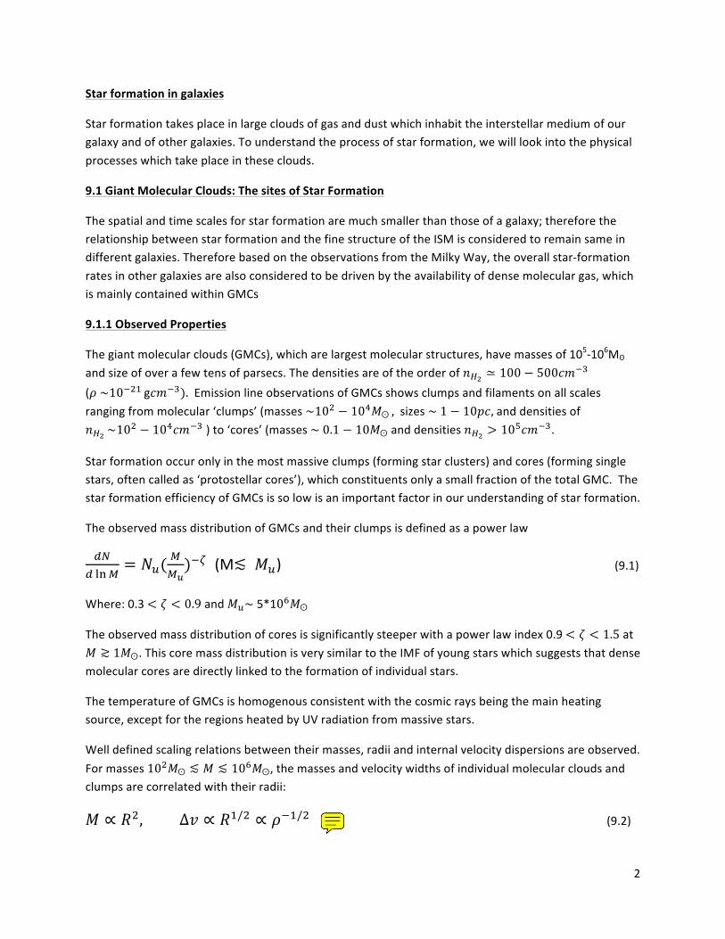
9.1.1 Observed Properties
The giant molecular clouds (GMCs), which are largest molecular structures, have masses of 105-‐106Mʘ
and size of over a few tens of parsecs. The densities are of the order of !!! ≃ 100 − 500!"!! (! ~10!!" g!"!!). Emission line observations of GMCs shows clumps and filaments on all scales ranging from molecular ‘clumps’ (masses ~10! − 10!!ʘ , sizes ~ 1 − 10!", and densities of !!! ~10
! − 10!!"!! ) to ‘cores’ (masses ~ 0.1 − 10!ʘ and densities !!! > 10!!"!!.
Star formation occur only in the most massive clumps (forming star clusters) and cores (forming single stars, often called as ‘protostellar cores’), which constituents only a small fraction of the total GMC. The star formation efficiency of GMCs is so low is an important factor in our understanding of star formation.
The observed mass distribution of GMCs and their clumps is defined as a power law
!"! !"!
= !!(!!!)!! (M≲ !!) (9.1)
Where: 0.3 < ! < 0.9 and !!~ 5*10!!ʘ
The observed mass distribution of cores is significantly steeper with a power law index 0.9 < ! < 1.5 at ! ≳ 1!ʘ. This core mass distribution is very similar to the IMF of young stars which suggests that dense molecular cores are directly linked to the formation of individual stars.
The temperature of GMCs is homogenous consistent with the cosmic rays being the main heating source, except for the regions heated by UV radiation from massive stars.
Well defined scaling relations between their masses, radii and internal velocity dispersions are observed. For masses 10!!ʘ ≲ ! ≲ 10!!ʘ, the masses and velocity widths of individual molecular clouds and clumps are correlated with their radii:
! ∝ !!, ∆! ∝ !!/! ∝ !!!/! (9.2)
3
The observed linewidths (about 10km!!! on GMC scale) are much larger than what is expected from simple thermal broadening (~0.2!"!!! !"# ! = 10!) indicates that GMCs and molecular clumps have high level of supersonic turbulence.
The strong spatial correlation with young star clusters (ages ≲ 10!!"), and weak correlation with older star clusters, indicates that the typical lifetime of a GMC is ∼ 10!!", much shorter than the typical age of a galaxy.
9.1.2 Dynamical State
Are the GMCs collapsing, expanding, or in a state of equilibrium?
1. Idealized case, where a GMC will collapse under its own gravity—free-‐fall collapse: Assumption: GMCs are self-‐gravitating, homogeneous, isothermal spheres of gas, with no potential turbulence and/or magnetic fields. The mass have to exceed the thermal Jeans mass in order for cloud to collapse,
!! = !!/!
!!!!
(!!!)!/!≃ 40!ʘ(
!!!.!!"!!!
)!( !!!!""!!!!)!!/! (9.3)
with mean molecular mass = 3.4*10!!"g
The equivalent to the Jeans mass is called the Bonnor-‐Ebert mass for an isothermal sphere in pressure equilibrium
!!" = 1.182 !!!
(!!!)!!= 1.182 !!!
(!!!!!)!! (9.4)
!ℎ!"! !!! = !"!! !" !ℎ! !"#$%&' !"#$$%"#
GMCs and molecular clumps both have masses that exceed !! !"# !!" . With no additional pressure force, the free fall time under which they collapse and form stars is given by:
!!"" = ( !!!"!!
)!! ≃ 3.6 ∗ 10! !"( !!!
!""!"!!)!!/! (9.5)
2. Isotropic turbulence in GMCs The sound speed !! , used in case 1 for the calculation of !! and !!" is replaced with effective speed of sound, !!,!""! = !!! + !! where ! is 1D rms velocity due to turbulent motion.
3. Presence of magnetic field, B: Equating potential energy of a cloud with magnetic energy yields a characteristic mass of
!ɸ ≡!!!
!"!!!!
!!!!!
≃ 1.6 ∗ 10!!ʘ!!!
!""!"!!
!! !!"!"
! (9.6)
4
Discussion and conclusion:
As shown above, physical processes such as an interstellar magnetic field or turbulence may affect the structure and the evolution of GMCs and therefore play an important role in regulating star formation efficiency.
9.5 Empirical Star-‐Formation Laws
Star-‐formation rate (SFR) in a galaxy can be described in terms of the mass in stars formed per unit time per unit area;
Σ* !∗!"#!
The gas consumption time is defined as !!" =∑!"#!∗
Observations are used to determined empirical star-‐formation laws, i.e. empirical scaling relations between Σ ∗ and certain ISM properties. One such relationship was studied by Schmidt is discussed below.
9.5.1 The Kennicutt-‐Schmidt Law
Star-‐formation rate (SFR) in a galaxy is empirically related to the surface density of gas, by a power law known as the Schmidt law of star formation:
∑* ∝ ∑!"#! (9.20)
where N ~ 2 (for observed distribution of HI and stars perpendicular to the galactic plane).
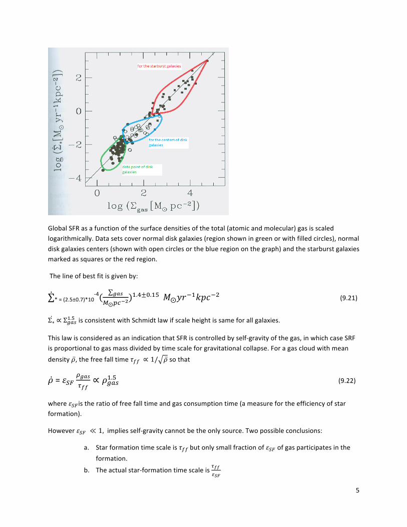
Schmidt law provides a very good fit of the global star-‐formation rates (averaged over the entire star-‐forming region) over a large range of surface densities (from the most gas-‐poor normal spiral galaxies as well as in the cores of the most luminous starburst galaxies) as shown in the plot below.
5
Global SFR as a function of the surface densities of the total (atomic and molecular) gas is scaled logarithmically. Data sets cover normal disk galaxies (region shown in green or with filled circles), normal disk galaxies centers (shown with open circles or the blue region on the graph) and the starburst galaxies marked as squares or the red region.
The line of best fit is given by:
∑* = (2.5±0.7)*10-‐4( ∑!"#
!⨀!"!!)!.!±!.!" !⨀!"!!!"#!! (9.21)
Σ∗ ∝ Σ!"#!.! is consistent with Schmidt law if scale height is same for all galaxies.
This law is considered as an indication that SFR is controlled by self-‐gravity of the gas, in which case SRF is proportional to gas mass divided by time scale for gravitational collapse. For a gas cloud with mean density !, the free fall time !!! ∝ 1/ ! so that
! = !!"!!"#!!!
∝ !!"#!.! (9.22)
where !!" is the ratio of free fall time and gas consumption time (a measure for the efficiency of star formation).
However !!" ≪ 1, implies self-‐gravity cannot be the only source. Two possible conclusions:
a. Star formation time scale is !!! but only small fraction of !!" of gas participates in the formation.
b. The actual star-‐formation time scale is !!! !!"
6
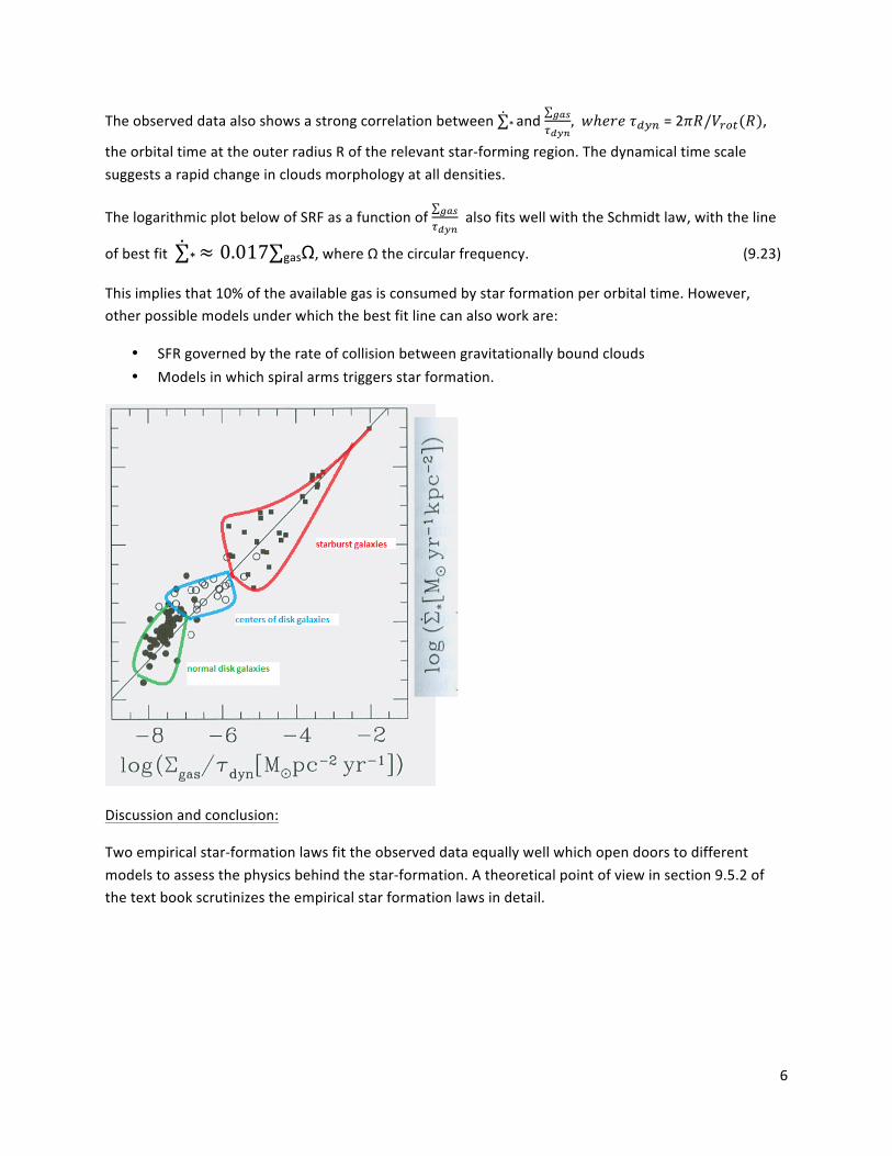
The observed data also shows a strong correlation between ∑* and ∑!"#!!"#
, !ℎ!"! !!"# = 2!"/!!"#(!),
the orbital time at the outer radius R of the relevant star-‐forming region. The dynamical time scale suggests a rapid change in clouds morphology at all densities.
The logarithmic plot below of SRF as a function of ∑!"#!!"#
also fits well with the Schmidt law, with the line
of best fit ∑* ≈ 0.017∑gasΩ, where Ω the circular frequency. (9.23)
This implies that 10% of the available gas is consumed by star formation per orbital time. However, other possible models under which the best fit line can also work are:
• SFR governed by the rate of collision between gravitationally bound clouds • Models in which spiral arms triggers star formation.
Discussion and conclusion:
Two empirical star-‐formation laws fit the observed data equally well which open doors to different models to assess the physics behind the star-‐formation. A theoretical point of view in section 9.5.2 of the text book scrutinizes the empirical star formation laws in detail.
7
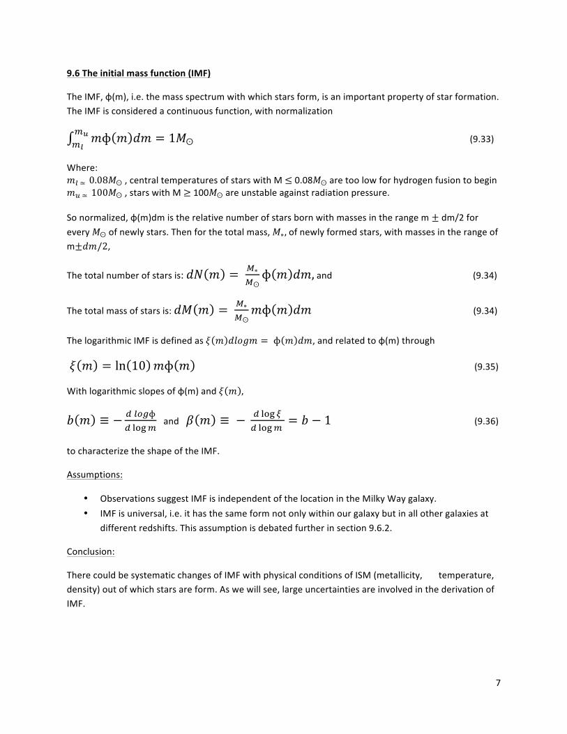
9.6 The initial mass function (IMF)
The IMF, ɸ(m), i.e. the mass spectrum with which stars form, is an important property of star formation. The IMF is considered a continuous function, with normalization
!ɸ ! !" = 1!ʘ!!!!
(9.33)
Where: !! ≃ 0.08!ʘ , central temperatures of stars with M ≤ 0.08!ʘ are too low for hydrogen fusion to begin !! ≃ 100!ʘ , stars with M ≥ 100!ʘ are unstable against radiation pressure. So normalized, ɸ(m)dm is the relative number of stars born with masses in the range m ± dm/2 for every !ʘ of newly stars. Then for the total mass, !∗, of newly formed stars, with masses in the range of m±!"/2,
The total number of stars is: !" ! = !∗!ʘɸ ! !", and (9.34)
The total mass of stars is: !" ! = !∗!ʘ!ɸ ! !" (9.34)
The logarithmic IMF is defined as ! ! !"#$% = ɸ ! !", and related to ɸ(m) through
! ! = ln 10 !ɸ ! (9.35)
With logarithmic slopes of ɸ(m) and ! ! ,
! ! ≡ − ! !"#ɸ! !"#!
and ! ! ≡ − ! !"# !! !"#!
= ! − 1 (9.36)
to characterize the shape of the IMF.
Assumptions:
• Observations suggest IMF is independent of the location in the Milky Way galaxy. • IMF is universal, i.e. it has the same form not only within our galaxy but in all other galaxies at
different redshifts. This assumption is debated further in section 9.6.2.
Conclusion:
There could be systematic changes of IMF with physical conditions of ISM (metallicity, temperature, density) out of which stars are form. As we will see, large uncertainties are involved in the derivation of IMF.
8
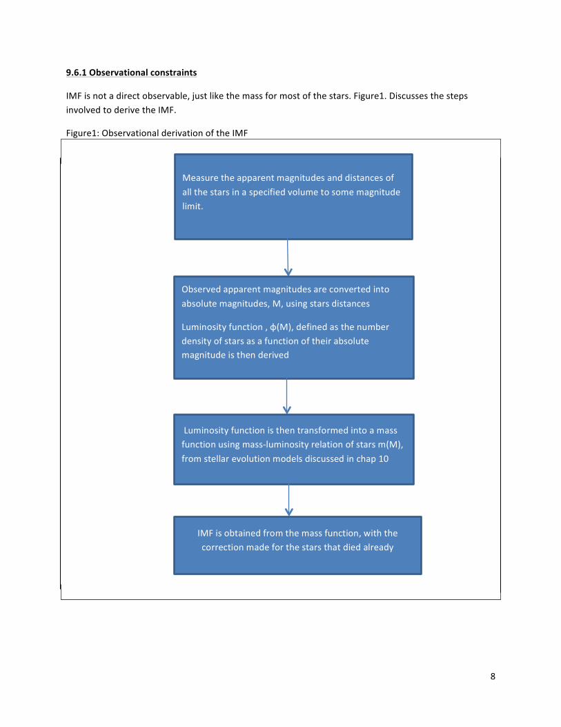
9.6.1 Observational constraints
IMF is not a direct observable, just like the mass for most of the stars. Figure1. Discusses the steps involved to derive the IMF.
Figure1: Observational derivation of the IMF
Measure the apparent magnitudes and distances of all the stars in a specified volume to some magnitude limit.
Observed apparent magnitudes are converted into absolute magnitudes, M, using stars distances
Luminosity function , ɸ(M), defined as the number density of stars as a function of their absolute magnitude is then derived
Luminosity function is then transformed into a mass function using mass-‐luminosity relation of stars m(M), from stellar evolution models discussed in chap 10
IMF is obtained from the mass function, with the correction made for the stars that died already
9
Time independent IMF:
The luminosity function, ɸ!, corrected for the stars that died already is given by equation (9.37):
ɸ! ! = ɸ ! ∗ ! ! !"!!
!
! ! !"!!!! !!!" !
(for !!" ! < !! )
!! ! = ! ! (for !!" ! > !! )
Where !!the present age of the Universe, and !!" ! is the main sequence lifetime of magnitude M star.
For stars with !!" ! < !! only fraction with ages younger than !!" can be observed, IMF then follows from
! ! ∝ !"!"!![! ! ] (9.38)
Sources of uncertainties in the observational derivation of the IMF
• For the conversion of observed apparent magnitude to intrinsic luminosity of a star, information of the distance of the star and the amount of extinction by intervening dust is required and reliable measurements can only be done for stars in small volume around the solar neighbourhood.
• Conversion from absolute magnitude to stellar mass, which are not always 1:1 related (especially for massive stars).
• Uncertainties involved in the determination of the star-‐formation history, !(t), affects the accuracy of the correction for the stars that have already died.
The IMF in our Galaxy
Various IMFs of our galaxy have been proposed by different investigators based on their studies:
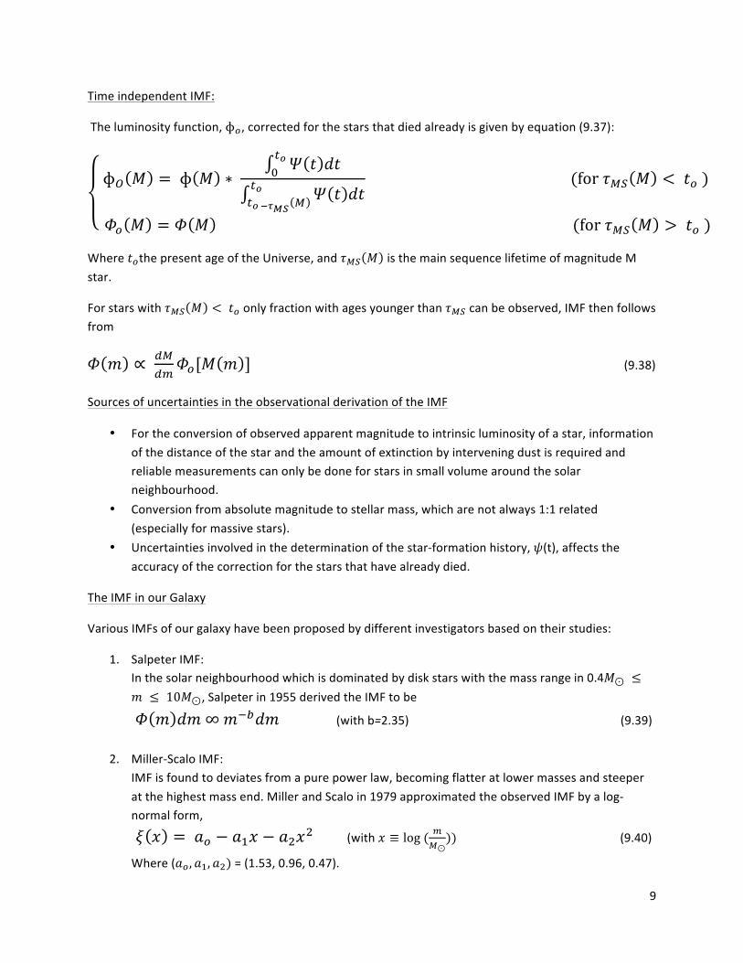
1. Salpeter IMF: In the solar neighbourhood which is dominated by disk stars with the mass range in 0.4!⊙ ≤! ≤ 10!⊙, Salpeter in 1955 derived the IMF to be
! ! !" ∞ !!!!" (with b=2.35) (9.39)
2. Miller-‐Scalo IMF: IMF is found to deviates from a pure power law, becoming flatter at lower masses and steeper at the highest mass end. Miller and Scalo in 1979 approximated the observed IMF by a log-‐normal form,
! ! = !! − !!! − !!!! (with ! ≡ log ( !!⊙)) (9.40)
Where (!! , !!, !!) = (1.53, 0.96, 0.47).
10
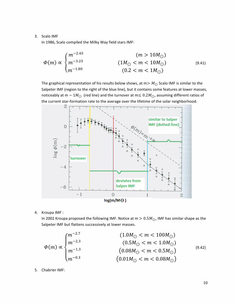
3. Scalo IMF
In 1986, Scalo compiled the Milky Way field stars IMF:
! ! ∝ !!!.!" (! > 10!⊙)!!!.!" (1!⊙ < ! < 10!⊙)!!!.!" (0.2 < ! < 1!⊙)
(9.41)
The graphical representation of his results below shows, at m> !⊙ Scalo IMF is similar to the Salpeter IMF (region to the right of the blue line), but it contains some features at lower masses, noticeably at m ~ 1!⊙ (red line) and the turnover at m≤ 0.2!⊙, assuming different ratios of the current star-‐formation rate to the average over the lifetime of the solar neighborhood.
4. Kroupa IMF : In 2002 Kroupa proposed the following IMF. Notice at m > 0.5!⊙, IMF has similar shape as the Salpeter IMF but flattens successively at lower masses.
! ! ∝
!!!.! (1.0!⊙ < ! < 100!⊙) !!!.! (0.5!⊙ < ! < 1.0!⊙)!!!.! 0.08!⊙ < ! < 0.5!⊙
!!!.! 0.01!⊙ < ! < 0.08!⊙
(9.42)
5. Chabrier IMF:
11
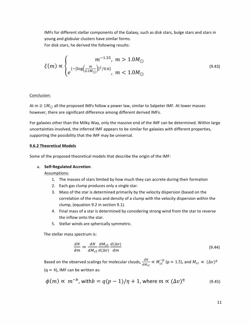
IMFs for different stellar components of the Galaxy, such as disk stars, bulge stars and stars in young and globular clusters have similar forms. For disk stars, he derived the following results:
! ! ∝!!!.!", ! > 1.0!⊙
!{![!"# !
!.!!⊙]!/!.!}
, ! < 1.0!⊙
(9.43)
Conclusion:
At m ≳ 1!⊙ all the proposed IMFs follow a power law, similar to Salpeter IMF. At lower masses however, there are significant difference among different derived IMFs.
For galaxies other than the Milky Way, only the massive end of the IMF can be determined. Within large uncertainties involved, the inferred IMF appears to be similar for galaxies with different properties, supporting the possibility that the IMF may be universal.
9.6.2 Theoretical Models
Some of the proposed theoretical models that describe the origin of the IMF:
a. Self-‐Regulated Accretion. Assumptions:
1. The masses of stars limited by how much they can accrete during their formation 2. Each gas clump produces only a single star. 3. Mass of the star is determined primarily by the velocity dispersion (based on the
correlation of the mass and density of a clump with the velocity dispersion within the clump, (equation 9.2 in section 9.1).
4. Final mass of a star is determined by considering strong wind from the star to reverse the inflow onto the star.
5. Stellar winds are spherically symmetric.
The stellar mass spectrum is:
!"!"
= !"!"!"
!"!"!(∆!)
!(∆!)!"
(9.44)
Based on the observed scalings for molecular clouds, !"!!!"
∝ !!"!! (p ≈ 1.5), and !!" ∝ (∆!)!
(q ≈ 4), IMF can be written as:
! ! ∝ !!!, with! = !(! − 1)/! + 1, where ! ∝ (∆!)! (9.45)
12
From assumption 4, the value of ! = 11/6 which yields an IMF slope ! ≈ 2.1, consistent with the observed value. However, observed stellar winds are typically collimated and therefore it is unclear to what extend results based on this model are applicable.
b. Hierarchical Accretion. If the stars form by accretion in self-‐similar networks of filaments over a wide range of scales, and if their masses are related to the masses of the fractal where they form, a power-‐law IMF can be produced. The number density of subclusters, with size l is: !"! !" !
∝ !!! where D is the fractal dimension of the cloud boundary. (9.47)
If the mass of a subcluster related to its size as ! ∝ !! then the mass function of a subcluster is !"
! !"!∝ !!!/! (9.48)
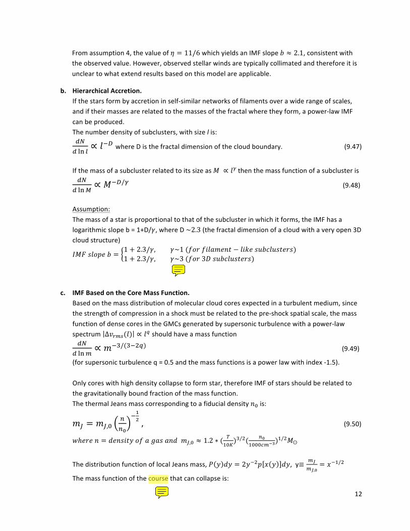
Assumption: The mass of a star is proportional to that of the subcluster in which it forms, the IMF has a logarithmic slope b = 1+D/!, where D ~2.3 (the fractal dimension of a cloud with a very open 3D cloud structure)
!"# !"#$% ! =1 + 2.3/!, !~1 (!"# !"#!"#$% − !"#$ !"#$%"!&'(!)1 + 2.3/!, !~3 (!"# 3! !"#$%"!&'(!)
c. IMF Based on the Core Mass Function. Based on the mass distribution of molecular cloud cores expected in a turbulent medium, since the strength of compression in a shock must be related to the pre-‐shock spatial scale, the mass function of dense cores in the GMCs generated by supersonic turbulence with a power-‐law spectrum ∆!!"#(!) ∝ !! should have a mass function !"
! !"!∝ !!!/(!!!!) (9.49)
(for supersonic turbulence q = 0.5 and the mass functions is a power law with index -‐1.5). Only cores with high density collapse to form star, therefore IMF of stars should be related to the gravitationally bound fraction of the mass function. The thermal Jeans mass corresponding to a fiducial density !! is:
!! = !!,!!!!
!!! , (9.50)
!ℎ!"! ! = !"#$%&' !" ! !"# !"# !!,! ≈ 1.2 ∗ ( !!"!
)!/!( !!!"""!!!!)!/!!ʘ
The distribution function of local Jeans mass, ! ! !" = 2!!!! ! ! !", y≡ !!
!!,!= !!!/!
The mass function of the course that can collapse is:
13
!"! !"!
∝ ! ! !"!/!!,!! !!!/(!!!!) (9.51)
Refer to appendix A for more details
d. (Non)-‐Universality of the IMF. Current observations are consistent with the idea of universal IMF on larger scales larger than individual star-‐forming regions. However, large uncertainties are involved.
1. Local variations of IMF in different star-‐forming regions. For example (Taurus no star massive than ~2!ʘ whereas Orion cloud contains both high and low mass stars).
2. Small and cold molecular clouds (< 10!) do not contain massive stars earlier than late type B stars, whereas massive warm clouds found to be associated with HII regions produced by massive stars.
3. Starburst galaxies with large amounts of concentrated gas are likely to enhance the formation of GMCs, which could lead to IMF significantly different than in normal spiral galaxies.
Discussion and conclusion:
The morphology and evolution of the GMCs may depend on the metallicity, ambient radiation resulting in redshift dependence of temperature, may result in different IMF depending on the different physical properties.
Our understanding of star-‐formation is based on observations which involve large uncertainties and limited knowledge of ISM in different galaxies (such as starburst). However, based on observed data from the Milky Way and nearby galaxies, various investigations are done on of SFR, IMF and the evolution of GMCs, and various theoretical models have been proposed to understand the star-‐formation. Star formation remains the topic of on-‐going research.
14
References:
1. Mo, H., Van den Bosch, F., & White, S. (. D. M. (2010). Galaxy formation and evolution. Cambridge ; New York: Cambridge University Press.
2. Ward-Thompson, D., & Whitworth, A. P. (2011). An Introduction to Star Formation. Cambridge: Cambridge University Press.
3. Palla, F., Zinnecker, H., Maeder, A., Meynet, G., & Schweizerische Gesellschaft für Astrophysik und Astronomie. (2002).Physics of star formation in galaxies. Berlin ; New York: Springer.
4. Smith, M. D. 1. (2004). The origin of stars. London: Imperial College Press.