Stansfield Localization Algorithm: Theoretical Analysis and Distributed Implementation

IEEE WIRELESS COMMUNICATIONS LETTERS, VOL. 2, NO. 3, JUNE 2013 327

Stansfield Localization Algorithm:Theoretical Analysis and Distributed Implementation

Jun Wang, Student Member, IEEE, Jianshu Chen, Student Member, IEEE, and Danijela Cabric, Member, IEEE

Abstract—In this letter, we focus on the Stansfield localizationalgorithm, which is a direction-of-arrival (DoA) fusion algorithmwith high accuracy and low complexity. We derive the meansquare error of the Stansfield algorithm with estimated DoAestimation error variance. Our derivation considers the statisticalvariation of DoA, as well as the impact of receive signal strengthvariations and node self-positioning error. In addition, we pro-pose a distributed implementation of the Stansfield algorithmbased on diffusion adaptation, which obtains accuracy compara-ble to its centralized counterpart and saves total transmit powerfor sufficient node density.

Index Terms—Stansfield algorithm, passive localization, DoAfusion, performance analysis, distributed algorithms.

I. INTRODUCTION

INFORMATION about primary user (PU) location couldenable several key capabilities in cognitive radio (CR)

networks including improved spatio-temporal sensing, intelli-gent location-aware routing, as well as aiding spectrum policyenforcement. The PU localization requires cooperation of CRsperforming passive localization, since they need to detect andlocalize non-cooperative PU in the whole coverage area ata very low signal-to-noise ratio (SNR) [1]. Prior researchon passive localization can be categorized into three classesbased on the types of measurements shared among sensors,namely Received-signal-strength (RSS), Time-difference-of-arrival (TDoA) and Direction-of-arrival (DoA) [2]. TDoA-based algorithms are not suitable for CR applications sincethey require perfect synchronization among CRs. Therefore,RSS and DoA-based algorithms are the proper choices for thePU localization problem. Furthermore, our earlier work showsthat jointly using RSS and DoA measurements significantlyoutperforms RSS-only and DoA-only schemes [1].

In this letter, we focus on the Stansfield algorithm which is aDoA fusion algorithm that uses RSS measurements to improveaccuracy [3]. Stansfield algorithm outperforms other practicalDoA fusion algorithms, such as maximum likelihood (ML)algorithm solved by iteration methods and linear least squarealgorithm, and closely approaches the Cramer-Rao bound forjoint RSS/DoA-based localization algorithms [1]. Prior workon theoretical analysis of the Stansfield algorithm assumesknowledge of DoA estimation error variance for each CRsensor, which serves as the weight for DoA fusion [4]. Asshown later in this letter, the DoA estimation error variance isa function of instant RSS and true DoA. However, in practicethe RSS for each CR is varying because of geometry andchannel effects (such as path-loss and shadowing), and the

Manuscript received January 19, 2013. The associate editor coordinatingthe review of this letter and approving it for publication was I. Guvenc.

The authors are with the Department of Electrical Engineering, Universityof California, Los Angeles, CA, 90095, USA (e-mail: {eejwang, jshchen,danijela}@ee.ucla.edu).

This work is supported by the National Science Foundation under GrantNo.1117600.

Digital Object Identifier 10.1109/WCL.2013.032013.130052

true DoA cannot be perfectly estimated due to measurementnoise. Therefore, the DoA estimation error variance needs tobe estimated, and assuming it a known constant makes theresults in [4] less practical.

We present the comprehensive theoretical analysis anddistributed implementation of Stansfield algorithm. First, wederive the mean square error (MSE) of the Stansfield algorithmwith estimated weighting, for a given CR placement. Ouranalysis not only considers the statistical variation of RSSand DoA, but also the impact of node self-positioning error.We then proceed with derivation of the asymptotic MSE ofthe Stansfield algorithm for uniform random CR placement.In the latter part of the letter, we propose a distributedimplementation of the Stansfield algorithm based on diffu-sion adaptation [5]. The proposed distributed algorithm onlyrequires information exchange among one-hop neighbors, andobtains close accuracy compared to its centralized counterpart.We then analyze the per node computational complexity andtotal transmit power of centralized and distributed Stansfieldalgorithm, and show that the distributed algorithm savestransmit power for sufficient node density.

II. SYSTEM MODEL

Assume N CRs cooperate to localize a single PU. 2-dimensional locations of the PU and the nth CR are denotedas �P = [xP , yP ]

T and �n = [xn, yn]T , respectively. Each

CR estimates its location either through GPS or coopera-tive methods resulting in estimates following the distribution�n = [xn, yn]

T ∼ N (�n, σ2�,nI2). Available measurements at

CRs are RSS and DoA. RSS measurement at the nth CR ismodeled as ψn � c0PTd

−γn 10−sn/10Watt, where PT is the PU

transmit power, c0 is the (constant) average multiplicative gainat reference distance, dn = ‖�n−�P ‖ is the distance betweenthe nth CR and PU, γ is the path loss exponent, and 10−sn/10

is the i.i.d. log-normal shadowing with sn ∼ N (0, σ2s ). There-

fore the mean and variance of the RSS measurements are givenby μψ,n = c

1/2ψ c0PTd

−γn and σ2

ψ,n = cψ(cψ − 1)c20P2Td

−2γn

respectively, where cψ = exp(

(ln 10)2

100 σ2s

). The true DoA

of the PU at the nth CR is θn � arctan( yP−ynxP−xn

). CRsperform array signal processing techniques, such as MUSIC[6], to obtain DoA estimates. The estimated DoA is commonlymodeled as θn � θn+vn [6], where vn ∼ N (0, σ2

θ,n) and σ2θ,n

is the DoA estimation error variance. We use the Cramer-Raobound of DoA estimation error variance using uniform lineararray (ULA) to model σ2

θ,n [7, Sec. III-B, Eqn. 20]

σ2θ,n =

6PM

(κ cos θn)2NsNa(N2a − 1)ψn

= β1

ψn

1

cos2 θn, (1)

where PM is the noise power, κ is a constant determined bythe signal wavelength and array spacing, Ns is the numberof samples, Na is the number of antennas, θn is the array

2162-2337/13$31.00 c© 2013 IEEE

328 IEEE WIRELESS COMMUNICATIONS LETTERS, VOL. 2, NO. 3, JUNE 2013

orientation with respect to the incoming DoA defined as θn �θn− θn, where θn is the orientation of the nth array, and β �

6PM

κ2NsNa(N2a−1) . RSS and DoA measurements are jointly used

to obtain PU location estimate �P � [xp, yp]T . The resulting

MSE is given by MSE � E

[‖�P − �P ‖2

].

The ML DoA fusion scheme is a nonlinear least squarefunction that has to be solved by iterative algorithms suchas Gauss-Newton method, which suffers from divergence [4].The Stansfield algorithm is a linear approximation of the MLfusion scheme resulting in [4]

�∗P ≈ argmin

�P

1

2

N∑n=1

1

σ2θ,n

[Δyn cos θn −Δxn sin θn

]2(2)

where Δxn � xP − xn, Δyn � yP − yn, and σ2θ,n is the

estimated DoA estimation error variance obtained by replacingθn with θn in (1). Note that we do not use estimated distancein the Stansfield formulation as in [4] since it is not availablewithout the channel information between the CR and PU,and (2) is a weak function of distance estimates [4]. TheStansfield algorithm can be solved in closed-form [1], andits geometry interpretation is based on minimization of theweighted summation of distances from �P to lines formed byeach CR location and its DoA estimate.

III. PERFORMANCE ANALYSIS OF CENTRALIZED

STANSFIELD ALGORITHM

1) MSE for a Given Placement: Our derivation is basedon perturbation analysis of the minimum of a given function[4]. Let’s first rewrite the Stansfield objective function (2) asJ(�P , η), where η � [x1, y1, ψ1, θ1, . . . , xN , yN , ψN , θN ]T

is the set of parameters subject to estimation errors. If weset η equal to η � [x1, y1, μψ,1, θ1, . . . , xN , yN , μψ,N , θN ]T ,the function J attains a global minimum at �P = �P (thecost function attains value zero at the true PU location ifthere is no measurement noise). Let η be perturbed byδη, then the point of global minimum of J is perturbedby a corresponding δ�P . Assume δη is a random variablewith zero mean and covariance matrix S = E[δηδηT ] =diag[σ2

�,1, σ2�,1, σ

2ψ,1, σ

2θ,1, . . . , σ

2�,N , σ

2�,N , σ

2ψ,N , σ

2θ,N , ]. The

second moment of δ�P can be obtained by the approximation[4] Σδ�P = E

[δ�P δ�

TP

]≈ Σ−1

1,gΣ2,gΣ−11,g , where

Σ1,g � ∂2J

∂�2

P

∣∣∣∣∣(�P ,η)

=c1/2ψ PT c0

β

N∑n=1

cos2 θndγn

vθnvTθn (3)

Σ2,g �(

∂2J

∂�P ∂η

)S(

∂2J

∂�P ∂η

)T ∣∣∣∣∣(�P ,η)

=cψPT c0

β

N∑n=1

(PT c0σ

2�,n

β

cos4 θn

d2γn+ c

1/2ψ

cos2 θn

dγ−2n

)vθnvTθn ,

(4)

and vθn � [sin θn,− cos θn]T , where the subscript g stands for

given placement. We skip detailed derivations due to spacelimitations. The MSE is given by MSEg = {Σδ�P }11 +{Σδ�P }22.

2) MSE for Uniform Random Placement: Numerical in-tegration or ensemble averaging need to be performed onMSE derived in Section III-1 to get the average accuracyfor random CR placements. In this section we characterizethe localization accuracy for the uniform random placementby deriving the closed-form asymptotic MSE for such case,using a technique that we developed in [1, Sec. IV]. Weassume the CRs that can hear the PU form a circle withradius R and are uniformly placed in the area. The CRsare placed independently within the area, which indicatesindependency among all θn’s, all dn’s, and pairs of θn anddn. For this scenario, the distributions of θn and dn are givenby θn ∼ U [0, 2π) and pdn(r) = 2r

(R2−R20), for R0 ≤ r ≤ R,

where R0 is a guard distance to avoid overlap between CRsand PU. We further assume the array orientation error isdistributed as θn = θn − θn ∼ U(−θT , θT ). Note that both(3) and (4) are written as summation of functions of randomvariables dn, θn, and θn. Using the law of large numbers,for large N , we can replace ensemble average with statisticalmean, obtaining

Σ1,u ≈ Nc1/2ψ PT c0

2βE

[cos2 θn

]E[d−γn

]I2 � λ1I2 (5)

Σ2,u ≈ NcψPT c02β

{PT c0σ

2�

βE

[cos4 θn

]E[d−2γn

]+c

1/2ψ E

[cos2 θn

]E[d2−γn

]}I2 � λ2I2 (6)

where the subscript u stands for uniform random placement.The expectations in (5) and (6) can be obtained throughintegrations of the PDF of dn and θn. Therefore, we canfurther simplify the second moment of δ�P as Σδ�P ≈ λ2

λ21

I2.The MSE for centralized Stansfield algorithm for uniformrandom node placement is thus given by MSEu ≈ 2λ2/λ

21.

IV. DISTRIBUTED STANSFIELD ALGORITHM

1) Algorithm Description: In this section we propose thedistributed implementation of Stansfield algorithm based ondiffusion adaptation [5], which minimizes, in a distributedmanner, a global cost function composed of a summation oflocal cost functions. The global cost function of the Stansfieldalgorithm is given by (2) as J(�P ) =

∑Nn=1 Jn(�P ). One can

verify that {Jn(�P )} is differentiable and strictly convex sothat J(�P ) is strictly convex and the minimizer �

∗P is unique.

Therefore, for each node n, we implement the followingadaptive-then-combine (ATC) procedure [5]

ϕn,i = �P,n,i−1 − μn∇�PJn(�P,n,i−1) (7)

�P,n,i =∑l∈Nn

wl,nϕl,i (8)

where �P,n,i is the local estimate at node n and iteration i, μnis the step-size, Nn denotes the neighborhood of node n, wl,nis the weighting of each neighboring node which is determinedby its estimated DoA error variance, and ∇

�PJn(�P ) is the

column gradient vector of Jn(·) relative to �P given by

∇�PJn(�P ) = 1

σ2θ,n

[Δxn sin θn −Δyn cos θn

]vθn

, where

vθn

�[sin θn,− cos θn

]T. Note that each node only has to

share its local estimate to its neighbor, therefore the networktraffic is further reduced.

WANG et al.: STANSFIELD LOCALIZATION ALGORITHM: THEORETICAL ANALYSIS AND DISTRIBUTED IMPLEMENTATION 329

2) Analysis of Communication Overhead: We analyze thetotal transmit power and computational complexity of central-ized Stansfield algorithm (CSA) and the proposed distributedStansfield algorithm (DSA). The minimum transmit power fora link of length d is obtained from our channel model asPt,min = Pr,mind

γ10s/10, where Pr,min is the minimumreceived power to correctly receive the message. For thecomputation complexity estimates, we assume the number ofoperations (OPS) for addition, substraction and trigonometricfunctions is 1; for multiplication and division is 10.

For CSA, each node needs to report 4 parameters, i.e. xn,yn, θn and σθ,n, to the fusion center, the total number ofmessages is thus 4N . For the transmit power consumption, weassume the fusion center is roughly at the center of a circlearea of radius R, and nodes are placed according to a uniformdistribution. In this case, the average total power consumptionis expressed as

E [Pt,c] = E

[N∑n=1

4Pr,mindγn10

sn/10

]≈ 8NPr,minR

γe(ln 10)2

200σ2s

(γ + 2),

(9)where in the second equality we use statistical mean to replacesum of realizations. The number of OPS for CSA comes fromcomputing the closed-form location estimates at the fusioncenter, which is O(202N).

For DSA, we denote Rc and I as the range for connectivityamong CRs and the averaged number of iteration, respectively.Each CR needs to broadcast three parameters, i.e. xP , yP andσθ,n, to its neighbors. Note that σθ,n only needs to be sharedonce while the PU location estimates need to be shared everyiteration. Therefore the total number of messages sent by eachCR is 2I+1. Due to the uniform assumption of CR placement,the averaged number of neighbors for each CR is N R2

c

R2 − 1.The distance from a specific CR to its neighbors satisfies thePDF of dn by replacing R with Rc and set R0 = 0. Thus theaverage total power consumption is obtained similar to (9) as

E [Pt,d] ≈ 2N(2I + 1)Pr,minRγc e

(ln 10)2

200 σ2s

(γ + 2). (10)

Combining the results in (9) and (10) we get the power ratio

η =E [Pt,d]

E [Pt,c]=

2I + 1

4

(RcR

)γ, (11)

which indicates that DSA consumes less power when the nodedensity is high, i.e., a small Rc is enough to ensure each CRhas enough neighbors to use a small number of iterations toobtain stable PU location estimates. The network number ofOPS for DSA to solve the diffusion adaptation algorithm ateach node is O(21N2I(Rc

R )2 + 96NI).

V. NUMERICAL RESULTS

We summarize the basic parameter settings in our simula-tions as follows. The CRs are uniformly placed in a circle ofradius R = 150m and protective region R0 = 5m, centeredaround the PU with location �P = [0, 0]T for simplicityand without loss of generality. The CR node positioningerror standard deviation σ�,n is 1m. The PU transmit powerPT is 20dBm (100mW), the measurement noise power PMis −80dBm (10pW), the path-loss exponent and shadowingvariance are γ = 4.2 and σs = 4dB respectively. The power

20 40 60 80 1001

1.5

2

2.5

3

3.5

4

4.5

5

5.5

6

Number of Nodes

RMSE(m

)

CSA(Simu), σs = 2 dB

CSA(Theo), σs = 2 dB









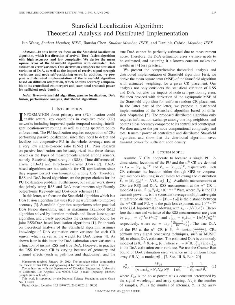
Fig. 1. Results for analytical and simulated RMSE of the Stansfield algorithmwith varying number of nodes, for different shadowing standard deviation σs.

and channel settings result in an averaged and minimumreceived SNR of 10dB and −10dB, respectively. Each CRis equipped with an ULA with Na = 2 antennas, and usesNs = 15 samples for each localization period. The arrayorientation error with regard to the incoming DoA is assumedto follow uniform distribution given by θn ∼ U(−π/3, π/3).Each data point in the figures is obtained by averaging1000 CR placements (with random array orientation) and2000 realization of RSS/DoA measurements. In the followingsubsections, we use these settings unless stated otherwise.

We first study the accuracy of the theoretical MSE of CSAfor a given placement derived in Sec. III-1 by plotting it versussimulation with varying number of nodes N , for differentshadowing standard deviation σs, as shown in Fig.1. Note thatwe use root-mean-square-error (RMSE) as the performancemetric which is obtained by taking square root of the MSE.We first observe that the Stansfield algorithm is robust toshadowing, since when σs changes from 2dB to 10dB, theRMSE is almost constant for any given number of nodes. Thisis because the log-normal PDF of the RSS ψn becomes morespread-out when σs increases, resulting in higher probabilitiesfor large RSS and small RSS observations. Since the DoAestimation error variances (1) are inversely proportional toRSS, increased shadowing results in more CRs with betterDoA measurements, as well as more CRs with worse DoAmeasurements. Therefore by assigning higher weights to CRswith better DoA measurements (i.e. larger RSS) in the DoAfusion process, we may obtain satisfying accuracy for largeshadowing cases. The theoretical RMSE closely approachesthe simulation for small and medium shadowing cases (i.e.,σs ≤ 6dB), while the gap becomes larger for large shadowing(i.e., σs ≥ 8dB). The reason is that the perturbation analysisused in Sec. III-1 is based on Taylor series expansion aroundzero point, which is more accurate for small errors in RSSand DoA. Note that when the number of node is greater than acertain threshold, i.e. 40, the theoretical MSE well approachessimulation for all values of σs.

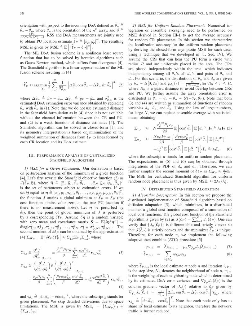
We then evaluate the robustness of the Stansfield algorithmto increasing node positioning error standard deviation σ�,nwith results shown in Fig.2. Note that we include the simulatedRMSE, theoretical RMSE averaged over random placements,as well as the asymptotic RMSE derived in Sec. III-2. Therequired number of CRs to make the asymptotic RMSEaccurate is affected by various array and channel parameters.

330 IEEE WIRELESS COMMUNICATIONS LETTERS, VOL. 2, NO. 3, JUNE 2013

1 1.5 2 2.5 3 3.5 40.5

1

1.5

2

2.5

3

3.5

4

4.5

Node Positioning Error Standard Deviation (m)

RMSE(m

)

CSA, Simu, N=40CSA, Theo, N=40CSA, Asym, N=40CSA, Simu, N=80CSA, Theo, N=80CSA, Asym, N=80

Fig. 2. Results for asymptotic RMSE, theoretical RMSE averaged overrandom placements and simulated RMSE of the Stansfield algorithm withvarying node positioning error standard deviation σ�,n, with uniform randomplacement of 40 and 80 nodes.

It is straightforward to numerically investigate impact of eachsystem parameter on the required N . Among all involvedparameters, we notice that R0/R, which corresponds to the‘forbidden region’ around the PU where activities of secondarynetwork will severely interfere with the PU, plays an importantrole in determining the required N . Our results show thatthe asymptotic RMSE provide satisfying accuracy for R0/Rgreater than 0.2 (i.e. forbidden area ratio greater than 4%),which is the setting used to obtain Fig.2. We observe fromthe figure that increased σ�,n causes a linear increase inthe RMSE. The gap between the theoretical RMSE averagedover random placement and the simulated RMSE becomeslarger when σ�,n increases, due to the inaccuracy of theTaylor series expansion for large node positioning errors. Wealso observe from Fig.2 that the asymptotic RMSE betterapproaches simulation for large number of nodes, as theprediction gap reduces from 1m to 0.1m when the numberof nodes changes from 40 to 80, under σ�,n = 3m.

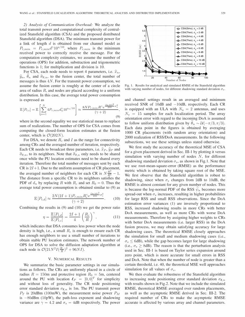
We then evaluate the accuracy of the distributed Stansfieldalgorithm and compare it with its centralized counterpart,for a specific uniform random placement of 40 nodes. ForDSA, each CR obtains an initial guess of the PU locationwith the following distribution �P,n,init ∼ N (�P , σ

2IGI2), and

the iteration at each node stops when norm of difference ofsuccessive iterations is less than 0.1m or the total numberof iterations reaches 100. Results for different combinationsof the connectivity radius Rc and the initial guess standarddeviation σIG are presented in Fig.3, in which the RMSE ofDSA is averaged over all CRs. It is observed that there isa tradeoff in the choice of step size μ: small μ results inslow convergence and less accuracy; while large μ causesdivergence. The optimal choice of μ is 10 for Rc = 75mand 18 for Rc = 100m, and it is independent of σIG. Notethat in the optimal step size region, DSA closely approachesthe accuracy of CSA for all simulated cases. We also observefrom our simulation that small Rc and large σIG result inlarge average number of iterations I at each CR, since eachnode has few neighbors and inaccurate initial guesses. Thevalues of I and the corresponding power ratios η calculatedfrom (11) are also shown in Fig.3. We conclude that DSAsaves power when Rc is small and the initial guess qualityis good (which effectively reduces I). In practical systems,the choice of Rc depends on the CR placement, and should

2 4 6 8 10 12 14 16 18 201

1.2

1.4

1.6

1.8

2

2.2

2.4

2.6

2.8

3

Step Size

RMSE(m

)

CSA, Theo.DSA, R

c=75m, σ

IG=10m (I=25, η=0.69)

DSA, Rc=75m, σ

IG=20m (I=30, η=0.83)

DSA, Rc=100m, σ

IG=10m (I=20, η=1.87)

DSA, Rc=100m, σ

IG=20m (I=25, η=2.32)

Fig. 3. Comparison of RMSE of centralized Stansfield algorithm withdistributed Stansfield algorithm with varying step size μ, for a fixed placementof 40 nodes.

ensure each node has enough neighbors to share information(at least 3 nodes according to our simulation). Therefore, wecan select small Rc with large node density, which results inmore power saving. Once the Rc is selected, the step size μcan be determined through off-line calibration process.

VI. CONCLUSION

In this letter we presented the comprehensive theoreticalframework for performance analysis of Stansfield algorithm,and its distributed implementation based on diffusion adap-tation. In the theoretical framework, we derived the MSEof the Stansfield algorithm as a function of estimated DoAestimation error variance. Our analysis not only considersthe statistical variation DoA, but also the impact of RSSvariations and node self-positioning error. Based on this result,we derived the asymptotic MSE of the Stansfield algorithmfor uniform random CR placement. Simulation results showthat the theoretical results closely match simulations. Thedistributed Stansfield algorithm obtains close performancecompared with its centralized counterpart, while requires in-formation exchange only among neighboring nodes and savestotal network transmit power for sufficient node density.

REFERENCES

[1] J. Wang, J. Chen, and D. Cabric, “Cramer-Rao bounds for jointRSS/DOA-based primary-user localization in cognitive radio networks,”accepted for publication in IEEE Trans. Wireless Commun., Dec. 2012.Available: http://arxiv.org/abs/1207.1469.

[2] N. Patwari, J. Ash, S. Kyperountas, A. Hero, R. Moses, and N. Cor-real, “Locating the nodes: cooperative localization in wireless sensornetworks,” IEEE Signal Process. Mag., vol. 22, no. 4, pp. 54–69, July2005.

[3] R. Stansfield, “Statistical theory of d.f. fixing,” J. Inst. of Electr. Eng.,vol. 94, no. 15, pp. 762–770, Mar. 1947.

[4] M. Gavish and A. Weiss, “Performance analysis of bearing-only targetlocation algorithms,” IEEE Trans. Aerosp. Electron. Syst., vol. 28, no. 3,pp. 817–828, Jul. 1992.

[5] J. Chen and A.H. Sayed, “Diffusion adaptation strategies for distributedoptimization and learning over networks,” IEEE Trans. Signal Process.,vol. 60, no. 8, pp. 4289–4305, Aug. 2012.

[6] P. Stoica and A. Nehorai, “Music, maximum likelihood, and cramer-raobound,” IEEE Trans. Acoust., Speech, Signal Process., vol. 37, no. 5, pp.720–741, May 1989.

[7] F. Penna and D. Cabric, “Bounds and tradeoffs for cooperative DOA-only localization of primary users,” in Proc. 2011 IEEE GLOBECOM,pp. 1–5.

Documents

Stansfield Localization Algorithm: Theoretical Analysis and Distributed Implementation