stanley’s Theory Of Magic Squares - Uppsalaqimh/Magic.pdf · Xantcha Stanley’s Theory of Magic Squares artist: A.D. The mathematician may be pleased to learn that the truncated

STANLEY’S THEORY OF MAGIC SQUARES

Qimh Richey Xantcha*

EAUMP Summer School on Combinatorial Commutative AlgebraArusha, 13th August – 21st August 2012

Mombi was not exactly a Witch, because the Good Witch who ruled that partof the Land of Oz had forbidden any other Witch to exist in her dominions. SoTip’s guardian, however much she might aspire to working magic, realized it wasunlawful to be more than a Sorceress, or at most a Wizardess.

L. Frank Baum: The Marvelous Land of Oz

This is an introduction to Magic Squares using the tools of CommutativeAlgebra, following Stanley: [4], [5], [6]. We lay no claims to originality, nordo we vouch for the correctness of these notes.

The prerequisites are rather modest: basic knowledge of graded rings andmodules, exact sequences, projective resolutions, and Hilbert’s Syzygy Theor-em.

§1. Magic Squares

Magic squares have spelt fascination to mankind throughout history and allacross the globe. The qualifying epithet “magic” is not simply an expressionof awe. Supernatural properties were indeed once ascribed to these objects.The Chinese legend of Lo Shu features a turtle wearing the pattern of a magic3ˆ3 square on its shell. Floor mosaics in India may sport a certain 3ˆ3 square,known as the Kubera-Kolam.

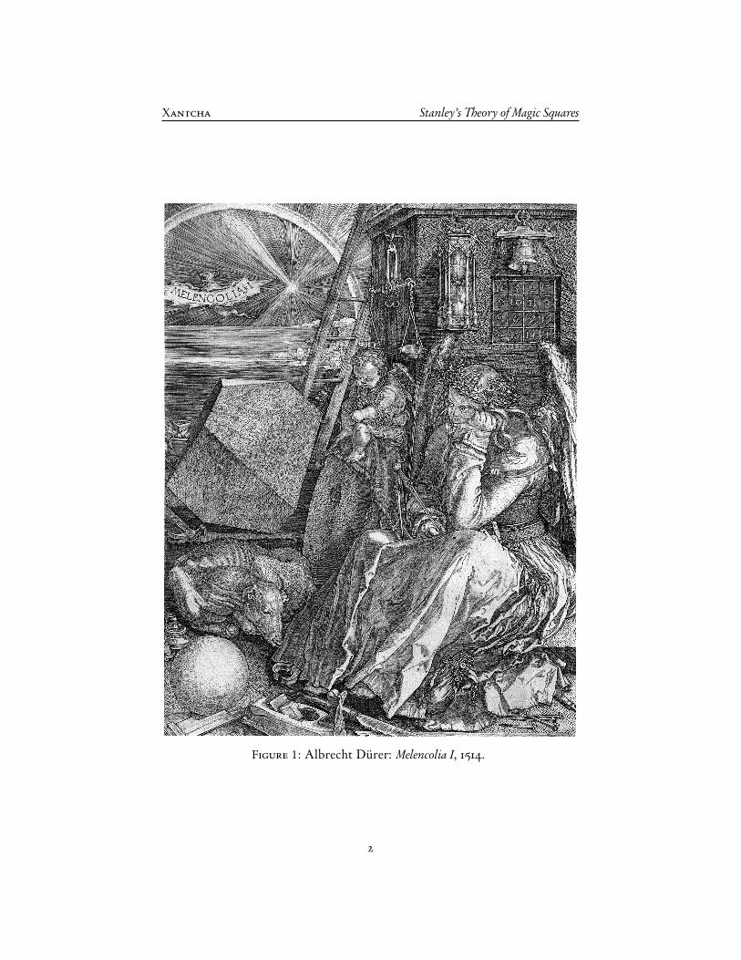
A famous specimen of measure 4 ˆ 4 has been immortalised in AlbrechtDürer’s engraving Melencolia I ; see Figure 1. Not only do the rows, columns,and main diagonals sum to 34; but also the little 2 ˆ 2 squares located inthe corners and at the centre. (The reader can, no doubt, exhibit still morequadruples in this square adding to 34.) The art-work is unusually ripe withthe exuberant symbolism of the Renaissance. For example, the middle twonumbers of the bottom row of the magic square read 1514, marking the exactyear of creation. The flanking entries, 1 and 4, encode the initials of the

*Qimh Richey Xantcha, Uppsala University: [email protected]

1

Xantcha Stanley’s Theory of Magic Squares

Figure 1: Albrecht Dürer: Melencolia I, 1514.

2


artist: A.D. The mathematician may be pleased to learn that the truncatedrhombohedron in the background has come to be known as Dürer’s solid, andits graph of vertices and edges as the Dürer graph.

There is an ever-ascending hierarchy of squares “more and more magical”.For example, Euler found a magic 8ˆ8 square, consisting of the numbers from1 through 64 arranged in such a pattern, that the sequence of numbers, takenin order, would form a knight’s tour on a chess board. One wonders how hewent about finding such a miraculous construction.

We shall be concerned with squares of admittedly very low magical poten-tial.

Definition 1. A magic square is a natural matrix whose row and columnsums all equal a fixed number, called the square’s magical number or magicalsum.

We shall denote by Hnpsq the number of nˆ n magic squares of sum s.

It will be the principal aim of these notes to study the properties of thefunctions Hn and derive explicit formulæ for low values of n.

Example 1. The number H1psq “ 1, for clearly`

s˘

is the only 1 ˆ 1 magicsquare of sum s. 4

Example 2. The number Hnp0q “ 1, for the zero matrix is the only magicsquare of sum 0. 4

Example 3. The number H2p1q “ 2, corresponding toˆ

1 00 1

˙

andˆ

0 11 0

˙

.

4

Example 4. Magic squares can be added, for example as in¨

˝

1 2 00 1 22 0 1

˛

‚`

¨

˝

4 1 22 3 21 3 3

˛

‚“

¨

˝

5 3 22 4 43 3 4

˛

‚,

where two magic squares of sums 3 and 7, respectively, produce a magic squareof sum 10. This extra structure will be exploited presently.

Compare with the definition of classical magic square in Problem 1.5. Themuch stronger property required for those squares will be destroyed underaddition. 4

Problems.

1. Determine the function H2.

2. Shew that the magic squares of sum 1 are precisely the permutation matrices,having exactly one 1 in each row and column, and 0 for the remainingentries. Use this to compute Hnp1q.

3


3. Calculate the number H3p2q.

4. Dropping the requirement that all entries be natural, allowing complexentries, the set of magic squares will then constitute a linear subspace ofthe space Cnˆn. Verify this and calculate its dimension.

5. A classical magic square of order n is an nˆn matrix meeting some harderprescriptions. It must contain specifically the numbers from 1 throughn2, and its rows, columns, and also main diagonals should sum to the samemagic number.

(a) What is the magic sum of a classical magic square of order n?(b) Find the number of distinct classical magic squares of orders 1, 2,

and 3, up to rotation and reflexion.(We remark that there are 880 squares of order 4, and exactly275, 305, 224 of order 5. There is no known formula generating thesenumbers. In particular, the number of classical magic 6ˆ 6 squaresis currently unknown, though estimated to be at around 1.7745¨1019.)

§2. Hilbert Series

Let A “À8

n“0 An be a complex algebra, commutative, associative, unital, andgraded over N. We assume it is finitely dimensional in each degree, and alsothat A0 “ C.

Modules over a graded ring are always assumed to be graded as well. Thatis, if M “

À8

n“0 Mn is a module over this A, then

AmMn Ď Mm`n.

Definition 2. Let M “À8

n“0 Mn be a module over the algebra A, finitelydimensional in each degree. Its Hilbert series is the formal power series

FMpλq “

8ÿ

n“0pdim Mnqλ

n.

Example 5. Consider the module M “ Crx, ys{px2, xyq, which is a moduleover the polynomial algebra A “ Crx, ys. Its components are given by:

M0 “ x1yM1 “ xx, yyM2 “ xy2y

M3 “ xy3y

...

The Hilbert series is

4


FMpλq “ 1` 2λ` λ2 ` λ

3 ` ¨ ¨ ¨ “ λ`1

1´ λ“

1` λ´ λ2

1´ λ.

4

Let a P A be a ring element and let M be a module over A. Define thesubmodule

aM “ t p P M | ap “ 0 u .

Lemma 1. Suppose a P Am, for some m ą 0. Then

FMpλq “FM{aMpλq ´ λ

mFaMpλq

1´ λm .

Proof. For a given n P N, consider the homomorphism a : Mn´m Ñ Mn. By theRank–Nullity Theorem,

dim Mn´m “ dim Ker a` dim Im a “ dim aMn´m ` dimpaMqn.

It follows that, for any n,

dimpM{aMqn ´ dim aMn´m “ dim Mn{paMqn ´ pdim Mn´m ´ dimpaMqnq“ dim Mn ´ dimpaMqn ´ dim Mn´m ` dimpaMqn“ dim Mn ´ dim Mn´m.

Consequently,

FM{aMpλq ´ λmFaMpλq “

8ÿ

n“0dimpM{aMqnλ

n ´ λm8ÿ

n“0pdim aMnqλ

n

“

8ÿ

n“0pdimpM{aMqn ´ dim aMn´mqλ

n

“

8ÿ

n“0pdim Mn ´ dim Mn´mqλ

n

“

8ÿ

n“0pdim Mnqλ

n ´

8ÿ

n“0pdim Mn´mqλ

n “ p1´ λmqFMpλq.

Example 6. Let us apply the lemma to the module Crx, ys{px2, xyq with a “y P Crx, ys. We have

M{yM “ x1y ‘ xxy ‘ 0‘ ¨ ¨ ¨

yM “ 0‘ xxy ‘ 0‘ ¨ ¨ ¨ ,

and so, once more, we arrive at the formula

FMpλq “FM{yMpλq ´ λFyMpλq

1´ λ“p1` λq ´ λ ¨ λ

1´ λ“

1` λ´ λ2

1´ λ.

4

5


Theorem 1 (Hilbert). Let A be generated by d elements of degree 1, and let M be amodule. Then

FMpλq “gpλq

p1´ λqd

for some integral polynomial gpλq.

Proof. If d “ 0, then A “ C, and the assertion is true, for FCpλq “ 1.Suppose now that A is generated by d elements of degree 1, among which

is a. The modules aM and M{aM are both annihilated by a, so they are in factmodules over A{aA, which is generated by d ´ 1 elements of degree 1. Hence,by induction,

FaMpλq “gpλq

p1´ λqd´1 and FM{aMpλq “hpλq

p1´ λqd´1 ,

and so, by the lemma,

FMpλq “FM{aMpλq ´ λFaMpλq

1´ λ“

hpλq ´ λgpλqp1´ λqd

.

Theorem 2. Let A be generated by d ě 1 elements of degree 1. For all sufficientlylarge n, the function

n ÞÑ dim Mn

is a rational polynomial of degree at most d ´ 1. It is called the Hilbert polynomial ofM.

Proof. dim Mn is the co-eHcient of λn in gpλq

p1´λqd. Let gpλq “

řmj“0 ajλ

j. Since

1p1´ λqd

“

8ÿ

j“0

ˆ

d ` j ´ 1d ´ 1

˙

λj,

we have

dim Mn “

mÿ

j“0aj

ˆ

d ` n´ j ´ 1d ´ 1

˙

for all n ě m, which is a polynomial in n of degree at most d ´ 1.

Example 7. The Hilbert polynomial of the module M “ Crx, ys{px2, xyq isthe constant function 1. 4

6


Problems.

1. Calculate the Hilbert series and Hilbert polynomial of the polynomialring Crxs.

2. Calculate the Hilbert series and Hilbert polynomial of the polynomialring Crx, ys.

3. Suppose a module has Hilbert series equal to the polynomial hpλq. Whatis its Hilbert polynomial?

4. If N is a submodule of M, shew that

FM “ FN ` FM{N .

5. Develop formulæ for the Hilbert series of the direct sum M ‘ N andtensor product M b N of two modules M and N .

§3. Linear Diophantine Systems of Equations

Consider an n ˆ n matrix X “ pxpqq of natural numbers. The condition for Xto be a magic square amounts to the following system of equations:

ÿ

i

xi1 “ÿ

i

xiq “ÿ

j

xpj, 1 ď p, q ď n.

The proper context is therefore as follows. Let D be an integral matrixwith k rows. We are seeking natural solutions to the linear system of equations

DX “ 0. (1)

Theorem 3. The solutions X P Nk to the linear system (1) form a commutativemonoid.

Proof. 0 is a solution, and if X and Y are solutions, then so is X ` Y .

Definition 3. A non-zero solution is said to be fundamental if it cannot bewritten as the sum of two non-zero solutions.

It is said to be completely fundamental if no natural multiple of it can bewritten as the sum of two non-zero, non-parallel solutions.

Example 8. Consider the system

`

1 1 ´2˘

¨

˝

xyz

˛

‚“ 0

and the three solutions p2, 0, 1q, p0, 2, 1q, and p1, 1, 1q. All three are fundamental,but only the first two are completely fundamental, for

2p1, 1, 1q “ p2, 0, 1q ` p0, 2, 1q.

4

7


Theorem 4 (Hilbert). There are only finitely many fundamental solutions, andevery non-trivial solution is a positive integral combination of such.

Proof. It is clear that any solution can be written as a positive integer combin-ation of fundamental solutions — just reduce a given solution until no longerpossible.

We now shew the number of fundamental solutions is finite. Consider firstthe case of a single equation, which we opt to write as

a1x1 ` ¨ ¨ ¨ ` amxm “ b1y1 ` ¨ ¨ ¨ ` bnyn,

where all the numbers ai and bi are positive, and, as always, we seek naturalsolutions.

Suppose yi ą a1 ` ¨ ¨ ¨ ` am. Then

a1x1 ` ¨ ¨ ¨ ` amxm “ b1y1 ` ¨ ¨ ¨ ` bnyn ą bipa1 ` ¨ ¨ ¨ ` amq,

so thata1px1 ´ biq ` ¨ ¨ ¨ ` ampxm ´ biq ą 0.

It follows that some xj ą bi. But if xj ą bi and yi ě aj, then the solution cannotbe fundamental, for the solution pxj, yiq “ pbi, ajq (all other letters equal to 0)may be deducted from it.

Consequently, in a fundamental solution, all variables yi ď a1 ` ¨ ¨ ¨ ` am,and similarly all xj ď b1 ` ¨ ¨ ¨ ` bn, and there can only be finitely many.

Suppose now that there are two equations. Write the solutions to the firstone as a natural combination of its fundamental solutions (which we know arefinitely many), with variable co-eHcients. Substituting this expression intothe second equation will yield a new integral equation in these co-eHcients,of which, by the argument just produced, has a finite number of fundamentalsolutions.

This procedure may be repeated for any given number of equations.

Theorem 5. There are only finitely many completely fundamental solutions, andevery non-trivial solution is a positive rational combination of such.

Proof. Since every completely fundamental solution is fundamental, their num-ber must also be finite.

Let the fundamental solutions be Q1, . . . , Qk. Then every solution can bewritten as a positive rational (in fact, positive integral) combination of these.

Suppose that Qk is not completely fundamental. We shall shew that somepositive multiple of Qk can be expressed as a positive rational combination ofQ1, . . . , Qk´1. Since Qk is not completely fundamental, there exists an m P Z`

such that

mQk “ pa1Q1 ` ¨ ¨ ¨ ` ak´1Qk´1 ` akQkq ` pb1Q1 ` ¨ ¨ ¨ ` bk´1Qk´1 ` bkQkq,

8


where some ai or some bj is non-zero, for 1 ď i, j ď k ´ 1. All co-eHcients arerational and non-negative. Collecting the terms containing Qk on one side ofthe equality yields:

m1Qk “ pa1Q1 ` ¨ ¨ ¨ ` ak´1Qk´1q ` pb1Q1 ` ¨ ¨ ¨ ` bk´1Qk´1q.

If m1 ď 0, there is a contradiction, for the right-hand side is certainly positive.Hence m1 ą 0, and we are done. A positive multiple of Qk, and therefore ofany solution, can be written as a positive combination of Q1, . . . , Qk´1 only.

Suppose now that Qk´1 is not completely fundamental either. Then thereexists a positive integer n such that

nQk´1 “ pa1Q1`¨ ¨ ¨àk´2Qk´2àk´1Qk´1q`pb1Q1`¨ ¨ ¨`bk´2Qk´2`bk´1Qk´1q,

where some ai or some bj are non-zero, for 1 ď i, j ď k´ 2. This yields

n1Qk´1 “ pa1Q1 ` ¨ ¨ ¨ ` ak´2Qk´2q ` pb1Q1 ` ¨ ¨ ¨ ` bk´2Qk´2q,

and again n1 ą 0.Repeat this procedure until only completely fundamental solutions re-

main.

Example 9. As an illustration of the technique, let us solve the system"

x´ 2z` w “ 0y´ 2z´ w “ 0

in accordance with the proof of Theorem 4.The first equation is easily seen to have the four fundamental solutions

px, y, z, wq “ p2, 0, 1, 0q, p0, 0, 1, 2q, p1, 0, 1, 1q, p0, 1, 0, 0q

and the general solution to this equation may be accordingly written

px, y, z, wq “ p2p` r, s, p` q` r, 2q` rq, p, q, r, s P N. (2)

Substitution of this into the second equation yields

0 “ y´ 2z´ w “ s´ 2pp` q` rq ´ p2q` rq “ ´2p´ 4q´ 3r ` s,

so that s “ 2p ` 4q ` 3r. Substituting back into (2) then yields the solution tothe system:

px, y, z, wq “ p2p` r, 2p` 4q` 3r, p` q` r, 2q` rq.

The three generating solutions are

P “ p2, 2, 1, 0q, Q “ p0, 4, 1, 2q, R “ p1, 3, 1, 1q.

It will be observed that they are all fundamental, but, since P `Q “ 2R, onlyP and Q are completely fundamental. 4

9


Problems.

1. Solve, in natural numbers, the diophantine system of equations"

2x` 3y´ z´ w “ 0x´ y´ z` w “ 0.

What are the fundamental solutions?

2. What is the number of fundamental solutions of the equation

a1x1 ` ¨ ¨ ¨ ` anxn ´ 2y “ 0,

where each aj P Z`?

§4. The Generating Function of a System of Equations

The objective is, as before, to study the natural solutions X P Nk of the systemof equations DX “ 0. These solutions form a commutative monoid, which wedenote by S.

Suppose that R1, . . . , Rq are solutions, and form the polynomial ring

A “ Crx1, . . . , xqs

in q indeterminates. The polynomial ring A is graded by the monoid S, wherebywe define deg xj “ Rj. This amounts to the following. The ring

A “à

PPSAP

splits up into graded components

AP “@

xm11 ¨ ¨ ¨ xmq

qˇ

ˇm1R1 ` ¨ ¨ ¨ `mqRq “ PD

, P P S;

and APAQ Ď AP`Q.

Example 10. Continuing the previous example, consider the three (funda-mental) solutions

P “ p2, 2, 1, 0q, Q “ p0, 4, 1, 2q, and R “ p1, 3, 1, 1q,

and form the polynomial ring A “ Crx, y, zs. We have, for example,

deg 1 “ 0 “ p0, 0, 0, 0qdeg x “ P “ p2, 2, 1, 0qdeg y “ Q “ p0, 4, 1, 2qdeg z “ R “ p1, 3, 1, 1q

deg x2y “ 2P `Q “ p4, 8, 3, 2q.

10


The graded components of A may be 0-, 1-, or 2-dimensional:

Ap0,0,0,0q “ x1yAp1,0,0,0q “ 0Ap2,2,1,0q “ xxy

Ap2,6,2,2q “ xxy, z2y .

4Next, define a module M over A as follows. As a vector space, M has a

complex basis consisting of all the elements of the monoid S (that is to say: allthe natural solutions to the system DX “ 0):

M “ CS “ xrPs | P P Sy .

The action of A on M is given by

xj ¨ rPs “ rRj ` Ps.

Defining the graded components of M to be 1-dimensional,

MP “ xrPsy , P P S;

it is easily verified that APMQ Ď MP`Q; i. e. M is a graded module over A.

Theorem 6. If R1, . . . , Rq include the completely fundamental solutions, the moduleM is finitely generated.

Proof. Suppose R1, . . . , Rq are completely fundamental, and consider the fi-nitely many fundamental solutions Q1, . . . , Qk. To each Qj there is an mj suchthat mjQj is a natural combination of the completely fundamental solutions.Then M is generated by the m1 ¨ ¨ ¨mq elements

ra1Q1 ` ¨ ¨ ¨ ` akQks , 0 ď aj ă mj.

For suppose w P M. Then w “ c1Q1 ` ¨ ¨ ¨ ` ckQk. Writing

cj “ gjmj ` aj, gj P N, 0 ď aj ă mj

givesw “

ÿ

j

gjmjQj `ÿ

j

ajQj.

Since mjQj is a natural combination of the completely fundamental solutions,we have

w “ÿ

i

hiRi `ÿ

j

ajQj

for some natural numbers hi. Consequently,

rws “ź

i

xhii

»

–

ÿ

j

ajQj

fi

fl .

11


Definition 4. The generating function of the system DX “ 0, is the formalpower series

f pλ1, . . . , λkq “ÿ

P

pdim MPqλP “

ÿ

PPS

λP “

ÿ

pp1,...,pkqPS

λp11 ¨ ¨ ¨ λ

pkk .

Example 11. Continuing the previous example, the generating function is

f pλ1, λ2, λ3, λ4q “ 1` λ21 λ

22λ3 ` λ

42 λ3λ

24 ` λ1λ

32λ3λ4 ` ¨ ¨ ¨

“ 1` λP ` λ

Q ` λR ` ¨ ¨ ¨

“ p1` λP ` λ

2P ` ¨ ¨ ¨ qp1` λQ ` λ

2Q ` ¨ ¨ ¨ qp1` λRq

“1` λ

R

p1´ λPqp1´ λQq.

This is no accident, as shewn by the subsequent theorem. 4

Theorem 7 (Stanley). The generating function f is a rational function, which,when reduced to lowest terms, is of the form

f pλq “gpλq

p1´ λR1q ¨ ¨ ¨ p1´ λRqq

,

where g is an integral polynomial and R1, . . . , Rq are the completely fundamental solu-tions.

Proof. When R1, . . . , Rq are the completely fundamental solutions, the mod-ule M is finitely generated, and so we may use Hilbert’s Syzygy Theorem toproduce a free resolution:

0 // Fq // Fq´1 // ¨ ¨ ¨ // F 1 // F0 // M // 0.

This sequence splits over the graded components into free resolutions:

0 // FqP

// Fq´1P

// ¨ ¨ ¨ // F 1P

// F0P

// MP // 0

for each P P S. By a well-known property of such sequences,

dim MP “ dim F0P ´ dim F 1

P ` ¨ ¨ ¨ .

Multiplying by λP and summing yields

f pλq “ f 0pλq ´ f 1pλq ` ¨ ¨ ¨ .

Suppose now Fp has free, homogeneous generators y1, . . . , yj. Then FpP has a

complex basis consisting of all elements

xa11 ¨ ¨ ¨ x

aqq yi, where a1R1 ` ¨ ¨ ¨ ` aqRq ` deg yi “ P.

12


Consequently,

f ppλq “

8ÿ

a1,...,aq“0

kÿ

i“1λ

a1R1`¨¨¨àqRq`deg yi “

řki“1 λ

deg yi

p1´ λR1q ¨ ¨ ¨ p1´ λRqq

,

and so f itself must be of the desired form.It remains to prove that the true denominator of f cannot be a proper

factor of the one given. By Problem 3 below, each polynomial 1 ´ λRj is irre-

ducible. Hence it will suHce to shew f cannot be written in the form

f pλq “gpλq

ś

j‰lp1´ λRj q

.

Suppose it can. For any r P N, the term λrRl must appear in the numerator

ppλq, because rRl P S and so must appear in the generating function. Hence,there is some term λ

U in the numerator gpλq and natural numbers bj such that

U `ÿ

j‰l

bjRj “ rRl.

Since U is a vector of natural numbers and all Rj P S, also U P S. From the factthat all Rj are completely fundamental solutions, it follows that

ř

j‰l bjRj “ 0,so U “ rRl. Having thus established that λ

rRl “ λU occurs in the numerator

gpλq for all r P N, we conclude that g cannot be a polynomial, but a properseries. This contradiction finishes the proof.

Problems.

1. Return to Example 10.

(a) Find more examples of graded components of A having dimensions0, 1, and 2, respectively.

(b) Do there exist components of A having dimensions greater than 2?

2. Shew that the generating function f of M may be viewed as a more finelygraded version of the Hilbert series, in the sense that putting λ1 “ ¨ ¨ ¨ “

λk yields the Hilbert series.

3. In the notation of the proof of Theorem 7, shew that each factor 1 ´ λR

is irreducible as long as R is a (completely) fundamental solution.

4. Find a criterion for M to be cyclic, that is, generated by a single element(which one?).

5. Prove the following converse to Theorem 6: If M is finitely generated,one can, among the Rj, find multiples of all the completely fundamentalsolutions.

13


§5. The Fundamental Magic Squares

Let G be a graph with vertices V pGq and edges EpGq. When A is a set ofvertices, denote by NpAq the set of neighbours of A, that is,

NpAq “ t v P V pGq | Du P A : uv P EpGq u .

Suppose now that G is bipartite, so that the vertices of G split up into twovertex sets U and V , with all edges running between these two sets.

Definition 5. Assuming |U| “ |V |, a perfect matching for G is a bijectionµ : U Ñ V such that uµpuq P EpGq for all u P U .

Theorem 8: Hall’s Marriage Theorem. G possesses a perfect matching if andonly if, for all X Ď U,

|NpXq| ě |X|. (3)

Proof. The condition is clearly necessary. To shew suHciency, we proceed byinduction on n “ |U| “ |V |. The case n “ 1 is trivial.

Case 1: For all A Ă U, one has |NpAq| ě |A| ` 1. Choose any u P U . Since|Npuq| ě |tuu| “ 1, the set Npuq is non-empty, and we choose a neighbourv P Npuq. The rest of the graph, Gztu, vu, is a smaller bipartite graph that willstill satisfy condition (3). Induction yields the result.

Case 2: There is some A Ă U such that |NpAq| “ |A|. Consider the followingtwo induced, non-empty, bipartite subgraphs of G:

H “ AY NpAq and K “ pUzAq Y pV zNpAqq.

For any set X Ď A, we have NH pXq “ NGpXq, so the graph H will satisfycondition (3). As for K, assume X Ď UzA. The equation

NGpX Y Aq “ NKpXq Y NGpAq

shews that

|X| ` |A| “ |X Y A| ď |NGpX Y Aq| “ |NKpXq| ` |NGpAq| “ |NKpXq| ` |A|.

Consequently, the graph K also satisfies the condition (3). Since the graphs Hand K are both smaller than G, we may conclude by induction.

Theorem 9: The Birkhoff–von Neumann Theorem. A magic square of magicsum s is the sum of s permutation matrices.

Proof. Consider an n ˆ n magic square Q. If Q “ 0, it is an empty sum ofpermutation matrices, so suppose Q ‰ 0. In keeping with the above notation,construct a bipartite graph G by letting U “ V “ rns, and including the edgeuv in G if and only if Quv ą 0. We leave it to the reader to verify that G fulfilscondition (3), and so we can apply Hall’s Marriage Theorem to find a perfectmatching µ : U Ñ V . This permutation µ satisfies Quµpuq ą 0 for all u P rns,and so the matrix Q ´ µ still has natural entries and will still be magic, ofmagic sum decreased by 1. We may then repeat the procedure until the zeromatrix is attained.

14


Theorem 10. The following conditions on a magic square Q are equivalent:

A. Q is fundamental.

B. Q is completely fundamental.

C. Q is a permutation matrix.

Proof. C implies B is clear, for a multiple of a permutation matrix, of minimalmagic sum 1, cannot be written as the sum of other magic squares. Also, Bimplies A is clear, for a completely fundamental solution is of course funda-mental. That A implies C follows from the Birkhov–von Neumann Theor-em.

Problems.

1. Write the matrix¨

˝

4 1 22 3 21 3 3

˛

‚

as the sum of permutation matrices. Can this be done in more than oneway?

2. Give an application to real life that would motivate the name MarriageTheorem!

3. Subdivide a standard deck of cards into thirteen piles, containing fourcards each. Shew that it is possible to choose one card from each pile, sothat, among the thirteen cards chosen, all the ranks from ace to king berepresented.

4. Complete the proof of the Birkhov–von Neumann Theorem, by veri-fying that the graph G indeed satisfies the condition of Hall’s MarriageTheorem.

5. Shew that magic squares can be multiplied, and the result will again bemagical. What is the magic sum of the product?

§6. Counting Magic Squares

Once more, we turn our attention towards

CS “ xrPs | P P Sy ,

though this time considered, not as a module, but rather as a ring in its ownright. Multiplication is given by the formula

rPs ¨ rQs “ rP `Qs

15


and the ring is N-graded by magic sum.It is almost uncanny what a simple inspection of this ring will yield. We

implore the reader to examine carefully the first three lines of the subsequentproof. Four lines only — in order to reach such a strong and triumphantconclusion! Surely this will convince the reader (if he were not already aholder of this conviction) of the power and glory of Abstract Algebra?

Theorem 11. The function Hn is a rational polynomial.

Proof. The ring CS is generated by elements of degree (magic sum) 1, viz. thepermutation matrices. The dimension dimpCSqs counts the number of magicsquares of sum s, and so an immediate application of Theorem 2 yields thatHnpsq agrees with a polynomial for suHciently large values of s.

To prove that Hn co-incides with this polynomial function everywhere, somedetailed analysis of the generating function will be required. Stanley’s originalproof is given in [4].

Theorem 12. The degree of Hn is exactly pn´ 1q2.

Proof. Consider a magic square Q “ pqijq of sum s. Each entry 0 ď qij ď s, andif qij is specified for all 1 ď i, j ď n´ 1, then the remaining entries are uniquelydetermined. This shews that

Hnpsq ď ps` 1qpn´1q2 ,

and so the degree of Hn cannot exceed pn´ 1q2.On the other hand, after arbitrarily choosing natural numbers

pn´ 2qspn´ 1q2

ď qij ďs

n´ 1, 1 ď i, j ď n´ 1;

the remaining entries (found by enforcing the magical property) are forced tobe natural. Hence

Hnpsq ěˆ

sn´ 1

´pn´ 2qspn´ 1q2

´ 1˙pn´1q2

“

ˆ

spn´ 1q2

´ 1˙pn´1q2

,

so that the degree of Hn must be exactly pn´ 1q2.

We record one auxiliary result before we put the finishing touch.

Theorem 13: Popoviciu’s Theorem ([3]). Let hpsq be a complex polynomial.Define

Fpλq “8ÿ

s“0hpsqλs and Fpλq “

8ÿ

s“1hp´sqλs.

There is an equality of rational functions:

Fpλq “ ´Fpλ´1q.

16


Proof.

Fpλq ` Fpλ´1q “

8ÿ

s“0hpsqλs `

8ÿ

s“1hp´sqλ´s

“

8ÿ

s“0hpsqλs `

´1ÿ

s“´8hpsqλs “

8ÿ

s“´8hpsqλs.

The equality of the theorem will be established once we have shewn that

8ÿ

s“´8sm

λs “ 0

for all m P N. We proceed inductively. The equality is true for m “ 0, for

8ÿ

s“´8λ

s “

8ÿ

s“0λ

s `

8ÿ

s“1λ´s “

11´ λ

`λ´1

1´ λ´1 “ 0.

Diverentiating this equation with respect to λ yields

8ÿ

s“´8sλs “

8ÿ

s“´8ps` 1qλs “

8ÿ

s“´8sλs´1 “ 0,

and so forth.

The Gorenstein property is a pleasant property for rings to possess, andthe notion is ubiquitous in Commutative Algebra. A precise definition isunfortunately beyond the scope of these notes, and we shall content ourselveswith recording the following facts:

1. The ring CS has the Gorenstein property and is of Krull dimension n.This was essentially proven by Hochster in [2].

2. When R is a Gorenstein ring of Krull dimension n, there is an integer gsuch that

FRpλ´1q “ p´1qnλ

gFRpλq.

This was proven by Stanley in [5].

3. For the ring CS, the number g “ n. There is a vague attempt at anexplanation in [6], which, unfortunately, makes no evort to trace theorigins of this illation.

Theorem 14. The polynomial Hn has the following properties, for all s P C:

Hnp´1q “ Hnp´2q “ ¨ ¨ ¨ “ Hnp´pn´ 1qq “ 0

andHnp´pn` sqq “ p´1qn´1Hnpsq.

17


Proof. By the enumerated list above and Popoviciu’s Theorem, the Hilbertseries Fpλq “

ř8

s“0 Hnpsqλs of the ring CS fulfils8ÿ

s“1Hnp´sqλs “ Fpλq “ ´Fpλ´1q “ p´1qn´1

λnFpλq “ p´1qn´1

λn8ÿ

s“0Hnpsqλs,

from which the theorem follows.

Example 12. The function H2 has degree 1 and satisfies H2p´1q “ 0 (fromthe theorem) and H2p0q “ 1 (easy). Hence it must be given by the formula

H2psq “ 1` s,

which was established by elementary means in an exercise. 4

Problems.

1. Determine H3.

2. Considering the information jointly provided by the above theorems,what is the minimum value of p, for which knowledge of the quantitiesHnp0q, . . . , Hnppq will suHce in order to deduce the polynomial Hn?

3. Give an algebraical proof that deg Hn “ pn´1q2 along the following lines.

(a) Shew that, if the space of all complex solutions to DX “ 0 has di-mension d, then the denominator of the Hilbert series

ř

pdim Mmqλm,

when reduced to lowest terms, is p1´ λqd .(b) Shew that this implies that the function m ÞÑ dim Mm is polynomial

of degree d ´ 1.(c) Now use Problem 1.4 to conclude the proof.

References

[1] David Hilbert: Ueber die Theorie der algebraischen Formen, Mathematische

Annalen Vol. 36, 1890.

[2] M. Hochster: Rings of invariants of tori, Cohen–Macaulay rings generated bymonomials, and polytopes, Annals of Mathematics 96, 1972.

[3] T. Popoviciu: Studie si cercetari stiintifice, Acad. R.P.R. Filiala Cluj 4, 1953.

[4] Richard P. Stanley: Linear Homogeneous Diophantine Equations and Magic La-belings of Graphs, Duke Mathematical Journal 40, 1973.

[5] Richard P. Stanley: Hilbert Functions of Graded Algebras, Advances in Math-

ematics 28, 1978.

[6] Richard P. Stanley: An Introduction to Combinatorial Commutative Algebra, inEnumeration and Design (D. Jackson and S. Vanstone, eds.), Academic Press1984.

18


Hints and Answers to Problems

1.1. H2psq “ 1` s.

1.2. Hnp1q “ n!.

1.3. H3p2q “ 21.

1.4. The dimension is n2 ´ 2n` 2.

1.5. (a) The magic sum is npn2`1q

2 .(b) The number of classical magic squares of order 1, 2, 3 is 1, 0, 1,

respectively. For the case 3 ˆ 3, begin by shewing the central entryhas to be 5.

2.1. 11´λ

and 1, respectively.

2.2. 1p1´λq2 and 1` n, respectively.

2.3. 0. The module contains only a finite number of non-zero graded com-ponents.

2.4. —

2.5. FM‘N “ FM ` FN and FMbN “ FM ¨ FN .

3.1. The fundamental solutions are p2, 0, 3, 1q and p0, 1, 1, 2q. The system ismost easily solved by starting with the second equation.

3.2. There are exactly n` kpk´1q2 fundamental solutions to the equation, where

k is the number of odd a’s.

4.1. (a) —(b) Yes, for instance: Ap4,12,4,4q “ xx2y2, xyz2, z4y.

4.2. —

4.3. Consider the special case of a single variable. A polynomial 1 ´ xr canonly reduce as

1´ xpq “ p1` xq ` x2q ` ¨ ¨ ¨ ` xpp´1qqqp1´ xqq,

where r “ pq.

4.4. M is generated by r0s if and only if R1, . . . , Rq include all the fundamentalsolutions.

4.5. The generators of M may be taken to be of the pure form rQs. Givenan element rPs P M, express rnPs, for any n P N, in the generators rQs,and use the fact that there are only finitely many rQs to shew that somenP can be written as a linear combination of these generators. Thenconsider what happens when P is completely fundamental.

19


5.1. Yes, it can.

5.2. —

5.3. Let U be the set of piles and V be the set of values.

5.4. —

5.5. Deploy the Birkhov–von Neumann Theorem. The magic sum of aproduct is the product of magic sums.

6.1. H3psq “ps`1qps`2qps2`3s`4q

8 .

6.2. p “ pn´1qpn´2q2 .

6.3. —

20

Documents

stanley’s Theory Of Magic Squares - Uppsalaqimh/Magic.pdf · Xantcha Stanley’s Theory of Magic Squares artist: A.D. The mathematician may be pleased to learn that the truncated