Embed Size (px)
Citation preview

The Methods of the Quality of Life Assessment
Stanislav Kolenikov
Scientific advisor:
Prof. S. A. Aivazian, RAS CEMI
NES, Moscow
1998
Abstract
This Master Thesis develops the concept of Quality of Life as an aggregate measure of people’s
well-being in a certain country, region, or social stratum. The historical approaches to the
quality of life measurement and estimation are given in the intorduction and literature review.
The United Nations approach to construction of a numerical measure of human development
(human development index) is presented. A simple regression model and ranking according to
the principal components of the set of economic and social indicators are proposed as ways to
quantify the quality of life given its expert estimates as a training sample. This methodology was
found to be an efficient one as indicated by sufficient statistical significance of both models. The
success of the model served as a basis for application to rank the regions of Russian Federation
according to the first principal component of the set of statistical indicators. Also, Pareto-
rankings of both international and Russian observations was proposed as a non-compensatory
measure of quality of life.1
1 c© Stanislav Kolenikov, NES/CEMI, 1998. E-mail: [email protected].
This Master Thesis is prepared and published in LATEX 2ε.
Contents
I Quality of Life Concept 4
II Approaches to Quality of Life 8
II.1 Subjective Individual Quality of Life Evaluation . . . . . . . . . . . . . . . . . . 8
II.2 Human Development Index:
An Aggregate Country-Level Measure . . . . . . . . . . . . . . . . . . . . . . . . 10
IIIQuality of Life Measurements 15
III.1 A Simple Regression Model . . . . . . . . . . . . . . . . . . . . . . . . . . . . . 16
III.2 Principal Components Analysis . . . . . . . . . . . . . . . . . . . . . . . . . . . 20
III.3 Application to Regions of Russia . . . . . . . . . . . . . . . . . . . . . . . . . . 23
III.4 Pareto classification . . . . . . . . . . . . . . . . . . . . . . . . . . . . . . . . . . 25
IV Conclusion 29
A Data 30
B Stepwise regression 34
C Principal components 35
D Rank correlation 37
E Pareto classification 40
F Rankings of Regions of Russia 42
References 46
3

I. Quality of Life Concept
Economics, as well as all other sciences, puts the motto “Make life better” on its banner. What
stands behind these words? What is “better”? What is “worse”? These questions lie in the
normative rather than positive plane, and answering them requires certain bravity in dealing
with eternal humanity problems.
The message of the word “quality” is compliance with previously formed judgements, or
standards of comparison. If you have never met with a tynerator1 you could never tell whether
the one you were presented with is a qualitative one. So when one ponders upon quality, it
means a comparison, putting objects side by side, finding the relevant attributes and ranking
the differences between them.
The term “Quality of Life” relates to the description and evaluation of the nature or con-
ditions of life of people in a certain country or region. Quality of life is formed by exogeneous,
with respect to an individual or a social group, forces like production technology, infrastruc-
ture, relations with other groups or countries, institutions of the society, natural environment,
and also by endogeneous factors including interaction within the society and values of a person
or a society. The effect of these factors is not necessarily constant over time; for instance,
environmental issues were paid relatively small attention a century ago while today ecology is
undoubtedly one of the main people’s concerns, and information technologies penetrating each
shpere of human existense were not existent at that time at all.
The impetus to the development of the means of the quality of life assessment and eval-
uation was given in 1960s owing to the Social Indicators Movement. In 1960s, lots of public
educational, social, ecological programs were initiated, and quantitative indicators to measure
their success (or failure) were of great need. This movement, in turn, was brought about by a
view in the society that life had in general become worse though the standards of living were
considerably improving. This work resulted in a series of publications by Census Bureau (Social
1Do you know what is it? Neither do I.
4
S. Kolenikov Quality of life assessment
Indicators, [1]) monitoring trends in society status, values, and people’s lives quality.
Parallelly, the quality of life concept has been used in the medical literature for a long time
to denote the state of the patient in the deviations from the psychic norm, during the after-
operational reabilitation, or in oncologic diseases [2]. The two approaches differ in the object of
investigation, the latter mainly focusing on the individual quality of life. We shall concentrate
on social and economic aspects of the quality of life, i. e., we shall put society or economy to
the center of our attention.
Two types of the quality of life measures, or indicators, are distinguished, namely, subjective
and objective ones. Also, expert estimations which combine both subjective and objective
approaches are also widely used.
The subjective indicators reflect subjective evaluations of people’s lifes. They represent
the microlevel of the quality of life data collected from the individual agents. The measurements
of this kind are essentially personal and based on the individual reports of one’s well-being and
responses obtained in sociologic surveys and investigations [3]. People are asked what they feel
about their life, its values, what they care about most, etc. The questionaries can sometimes
contain up to a hundred of questions. Also, these data can be collected during a longitudional
investigations of the population [4]. Subjective measures reflect both the real status of the
quality of life, or the conditions of life in general, and the attitude of the people toward these
conditions. The aggregation of these subjective measures by statistical techniques and methods
can help identifying the values of society or different social groups.
The objective quality of life measures are built on the basis of “hard variables”, i. e., the
data from the municipal or governmental institutions and organizations which may include
financial accounts, civil state records, medical statistics, pollution levels, and other pieces of
information gathered by the institutions routinely. This approach aims at investigating the
society as a whole by looking, in the most general sense, at the set of macroeconomic, social,
demographic indicators which determine the conditions of life and the way people live.
As an objective measure, the quality of life may be defined as an interrelation of the four
determinants of the vital functioning and activity of the population [5]. These are the quality
of population, material welfare, the quality of the social system, and the quality of ecology,
or environment. The hierarchical decomposition of every component can go down to the basic
low-level characteristics assessed by the statistical data or by expert estimation. E. g., the
quality of population is inferred from the population demographic structure, the reproductive
5
S. Kolenikov Quality of life assessment
process and marital behavior, the population physical, psychic, and moral health, educational
level and proficiency. The material welfare is determined by the standards of living, income
differentiation, housing, telecommunication, trade, education, culture, health system, mass
media capacities. The social system quality relies upon the state and/or private provision in
cases of the (permanent or temporary) disablement, citizens’ rights for education, employment,
recreation, private property and personal protection, political system stability, individual’s
inclusion to the social infrastructure, race and sex equality, social stability. The ecology state is
influenced by the state of air and water basins, the level of chemical, radioactive, heavy metal
pollution, etc. The list is far from being complete, and some items may be related to more
than one category.2
So, each of the mentioned properties and measures, being expressed via a system of statistic
indicators, should then be integrated into a measure of the overall quality of (the particular
sphere of) life. It may also be required that the final aggregate measure satisfy the property
of uncompensatory preference, i. e., shortcomings in one of the fields cannot be compensated
by improvements in others. This requirement induces Pareto ranking in the phase space.
Commonly used linear or log-linear weighted combinations do not satisfy this property.
The methodology of decomposition, or introduction of a “phase space” [6] is often used
in related publications to assign the dimensions for factor scaling, with a more distant goal
of multicriterial ranking [7]. A very similar approach is proposed in [8] where five integral
indicators are proposed for estimating strategic decisions on regional level. Four of them next
to coincide with earlier proposed factors and relate to demography, welfare, environment, and
social comfort; the fifth indicator characterizes self-sufficiency of the region.
As another instance, Institute for Managerial Development (Lausanne) picks out eight main
spheres of intercountry comparison [9]: domestic economy strength, internationalization, gov-
ernment, finance, infrastructure, management, research and development, and people. Each of
the factors is then split down to specific criteria of the lowest level representing statistical data
2 In this context it is worth reminding a buddhist parable [23] about blind men who tried to perceive what
an elephant is. One touched the trunk and said, “An elephant is long and flexible”. Another touched the tusk
and said, “No, it is stern and sharp”. Yet another stood under the belly and said, “It is somewhat tall and
feels quite heavy” while the fourth stood behind holding the tail and concluded that an elephant was light and
smelled . . . hm . . . not very pleasant. What did they miss? Wholeness: an elephant is all these things taken
together.
6
S. Kolenikov Quality of life assessment
or expert estimates; the book reports about 250 indicators in the eight fields cited above.
The provision of information for quality of life analysis requires collection both the data de-
scribing separate aspects of life and integral characteristics of the social and human existense in
general. To correspond the problem of the quality of life improvement, the system of indicators
is to be built on the hierarchy principle since monitoring of a large number of indicators (i. e.,
statistical data) seems to be an ungovernable task. The lowest level of this system consists of
the sources, or basic statistical indicators, groupped according to separate fields of quality of
life analysis. At upper level, this basic data are used to calculate the aggregate measures of
the quality of life as a complex phenomenon. In the process of the aggregation, the unification
of non-related and non-commensurable indicators is required which implies the use of expert
and heuristic procedures. As a result, at the higher level of aggregation the estimates of the
quality of life tend to be only relative measures, thus being referred to as integral estimates, or
integral indicators, of the quality of life.
The expert estimation of the quality of life is carried out via comparison of the different
countries, or different regions or cities of the same country, by the group of experts. The final
data may be represented as an arbitrary numerical scale where the quality of life in the country
is given some numerical value; the ordered scale where all countries are ranked in decreasing
order, but without any numbers attached, or the matrix of pair comparisons where each two
countries are compared. The case of numerical scale is the simplest one since it allows for
regression models to be built. The two other types of data are substantially more difficult to
be analysed [10, 12].
The literature on the subjective methods of the quality of life assessment will be overviewed
in Section II.1. Section II.2 will concentrate on UN proposed measure of human development.
Section III.1 will contain a simple regression analysis based on objective and expert-estimated
variables. The necessary numerical data as well as mathematical methods description will be
dealt with in Appendices.
7

II. Approaches To Quality of Life: An
Overview
II.1 Subjective Evaluation: Data at
Individual Microlevel
The subjective quality of life assessment has been studied in sociologic and, to some extent,
economic literature for many years. The list of papers and books is quite exhaustive. The search
system of the Library of Congress (http://lcweb.loc.gov) supplies about 1100 references for
the request on the key words “Quality of life”. The bulk of literature is dated by 1970s
when the quality of life and other social issues were on the top of the public interest.
An examplary investigation to the quality of life is [13]. In this book the analysis of the
quality of life perception by American citizens is carried out by using the US statistical data on
both subjective evaluation of the quality of life in terms of happiness and satisfaction in most
important areas of human life, and objective indicators of material well-being and individual
resources. The semantic aspects of the response interpretation and corresponding significance
of statistical inference is paid a lot of attention. Along with the major component identification
(similar to the procedure of Section III.1), the time-trends in the general sense of well-being
are also analysed. The peculiarities of the quality of life analysis for the social groups such as
women and national minorities.
One of the most popular aggregate measures of the quality of life is the individual estimation
of one’s happiness. The concept of happiness has been paid attention by the leading thinkers
since antique times. Modern approach, though, implies the accurate definition of the terms and
construction of models for the applicable fields of study. According to this scheme, [14] distin-
guishes four main aspects of happiness inferred from the philosophic and scientific literature:
8
S. Kolenikov Quality of life assessment
happiness as possession (epicurism), happiness as satisfaction of needs and requirements (utili-
tarism), happiness as self-realization (eudemonism), happiness as a positive result of comparison
with other individuals and past experience (modern sociology). The results of empirical inves-
tigations conducted by the authors suggest that the degree of happiness is mainly explained,
in the statistical sense, by the positive evaluation of life situations and beneficial comparisons
with those of other individuals and past experience. Individual characteristic and resources at
his disposal (gender, age, income) affect happinnes indirectly, via processes of evaluation and
comparison.
Overwhelming are bibliographies [15] and [16] which index sociologic and philosophic lit-
erature related to subjective happiness. In the introduction to the latter source, concept of
happiness is defined as follows: “Happiness is defined as the degree to which an individual
judges the overall quality of her/his life as-a-whole favorably.” This enormous book contains
2472 references on subjective life perception covering the period from the Socrate and Plato
till the most modern studies. The author notes that the investigations on happiness were con-
ducted in different branches of social sciences: in ideologic, philosophic, morale and modern
scientific (sociologic) literature. The latter cluster of sources can hardly be analysed or even
accompanied since this literature is not well documented and spread around in different fields of
studies. Often happiness is a by-product of another research and, hence, not included into the
title and keywords of a paper. Nevertheless, English, French and Danish literature is described
quite extensively.
Another approach was used in the study “Cross-cultural quality of life research: an outline
for a conceptual framework” by E. Hankiss, R. Manchin, and L. Fustos published in routine
UNESCO publication [17]. A conceptual framework of economic flows and filters was outlined
which determine how the actions of agents is reflected in the quality of life both objective and
subjective. These filters are determined by institutions of the society and may include the
values of society and individuals, functioning of the public distributional system, direction of
time, life cycles, dominance of the society survival under conditions of exogenous influences
(i. e., wars or natural catastrophes), the life goals of an individual.
I cannot go without mentioning the materials developed in our research group headed by
Prof. S. A. Aivazian at Central Economics and Mathematics Institute of Russian Academy of
Science (RAS CEMI). He has been interested in the problems of statistical analysis of income
9
S. Kolenikov Quality of life assessment
distribution, consumption behavior and consumer preference reconstruction, as well as other
applications of mathematical statistics in social sciences, since he joined CEMI in late 1960s.
Now our group is working on a project with Goskomstat (State Committee on Statistics, Russian
Federation) which aims at developing a methodological framework for routine quality of life
analysis in Russia in the course of Goskomstat surveys [5].
II.2 Human Development Index:
An Aggregate Country-Level Measure
Human development index is a popular quantitative measure of the degree of a country’s
success in developing its human potential. Its introduction in early 90th was caused by the
necessity to find the measure of human progress which is people rather than economic-centred.
Economic growth does not necessarily imply human development, as well as a strong human
potential is not always reflected in economic performance, but in general these factors act
as mutually reinforcing entities, and this bilateral influence can additionally be magnified by
proper government policies.
Since 1990, United Nations Development Programme (UNDP) has been publishing annual
its “Human Development Report” [19] which explores in detail the relationship between human
development and “hard variables” representing the economic, social, demographic state of the
society. This program aims at revealing the relative performance of different countries via
constructing a numerical measure of human development. Of course, the concept of human
development is much deeper and richer than what can be captured in a composite index or
even by a detailed set of statistical indicators. Yet it is useful to aggregate different aspects of
a complex reality.
Though simple in construction, human development index (referred to as hdi further on)
provides useful insights into the causes of the differences between countries’ position in the world
ranking, and even may be used as a policy target. It also reveals very sharply the structure
and direction of the progress (or retrogression) in human potential in the course of economic
growth of a country, and the problems accompanying this progress across approx. 170 countries
for which necessary data are available.
10
S. Kolenikov Quality of life assessment
The hdi index reflects achievements in basic human capabilities in three fundamental dimen-
sions — a long and healthy life, an adequate education, and a decent standard of living (which
are related, to some extent, to the factors contributing to the quality of life as introduced on
page 5, namely, the material welfare, quality of population and social system quality). The
variables representing these three dimensions are life expectancy, educational attainment and
income. The hdi value for each country (region, etc.) indicates how far it has to go to attain
certain defined goals: an average life span of 85 years, access to education for all and a standard
of living on the world level. In fact, hdi weights deprivation in these three factors, i. e., the
relative distanse from the desirable goal on the unit scale.
For any component of the hdi, individual indices are computed according to the general
formula:
Index =Actual valuei −Minimum valuei
Maximum valuei −Minimum valuei(II.1)
Fixed minimum and maximum values have been established for each of the indicators:
• Life expectancy at birth: 25 and 85 years;
• Adult literacy: 0% and 100%;
• Combined enrolment ratio: 0% and 100%;
• Real GDP per capita (PPP$): PPP$100 and PPP$40000.
Educational attainment index is built as a linear combination of adult literacy and combined
primary, secondary and tertiary enrollment ratios with weights 2/3 and 1/3, respectively:
Educational attainment =2
3Adult literacy +
1
3Combined enrollment (II.2)
The construction of the income index is more complex and is based on the utility of income
with varying elasticity:
W (y) =
y ∀ y : 0 < y < y∗,
y∗ + 2[(y − y∗)1/2] ∀ y : y∗ ≤ y ≤ 2y∗,
y∗ + 2(y∗)1/2 + 3[(y − 2y∗)1/3] ∀ y : 2y∗ ≤ y ≤ 3y∗,
etc.
(II.3)
11
S. Kolenikov Quality of life assessment
where y∗ is a threshold level of income. For international comparison, y∗ is taken to be the
average world income. In [19] (1996) the value of PPP$5711 is cited as an average world income
in 1996. Consequently, the utility of maximum (target) income, PPP$40000, or adjusted real
GDP per capita, would be
W (40000) = y∗ + 2(y∗)1/2 + 3(y∗)1/3 + 4(y∗)1/4 + 5(y∗)1/5+
6(y∗)1/6 + 7(y∗)1/7 + 8[(40000− 7y∗)1/8] = PPP$6040.
The hdi is an average of the life expectancy, educational attainment and the adjusted real
GDP per capita (PPP$) indices, i. e., the sum of the indices divided by three:
HDI = (Life expectancy index + Education attainment index+
Adjusted income index)/3(II.4)
Thus this is a composite comparative index reflecting relative performance of a country or a
region as compared to some fixed standards.
The methodology of the hdi calculation is very young and still in the process of formation.
For instanse, [19] (1995) notes: “Since Human Development Report 1994, two changes have
been made in the construction of the HDI relating to variables and minimum and maximum
values. First, the variable of mean years of schooling has been replaced by the combined primary,
secondary and tertiary enrolment ratios, mainly because the formula for calculating mean years
of schooling is complex and has enormous data requirements . . . Second, the minimum value
of income has been revised from PPP$200 to PPP$100”. Threshold level of income y∗ is also
changing with time. So it makes sense to state explicitly which data, maximum and minimum
values, threshold levels were used in computing hdi.
Gender-Related Development Index
The methodology of hdi calculation allows for adjustment for inequality in positions of different
population groups, e. g., men and women. The general assumptions underlying the construction
of gdi (gender-related development index) are those of equality in potentials of the two group
except for the longevity which is known to be higher for women, and of social preference for
equality represented by a specific weighting formula. Another assumption should also be made
related to the sources of income when considering gender income discrimination that the ratio
of non-labor income to labor income is the same across population.
12

S. Kolenikov Quality of life assessment
With gender-adjusted maximum and minimum life expectancy values (87.5 and 27.5 years
for women; 82.5 and 22.5 years for men), the same formulas (II.1)–(II.4) are used to calculate
partial men and women related partial indices.
Different approaches could be taken to account for the gender difference obtained on the
previous step. The simplest one is to multiply the hdi by the ratio of the female hdi to the male
one. This used to be an early approach found in [19] (1993). Later, it was substituted to a
more complicated one.
Since 1995, UNDP have been exploring the extension of the approach of [20] with risk, or
inequality, aversion. Let X be an indicator of achievement, and let Xf and Xm refer to the
corresponding female and male achievements. If nf and nm are the numbers of females and
males in the population, the overall or mean achievement X is given by
X = (nfXf + nmXm)/(nf + nm) (II.5)
This mean achievement is compared to an “equally distributed equivalent achievement” Xede
defined as the level of achievement which is socially equivalent to the actually observed vector
(Xf , Xm). Social valuation is defined by the concave function with constant elasticity:
V (X) =
X1−ε − 1
1− ε, ε ≥ 0, ε 6= 1
lnX,ε = 1
(II.6)
Xede is thus defined through
(nf + nm)X1−εede
1− ε= nf
X1−εf
1− ε+ nm
X1−εm
1− ε(II.7)
or, after simplification,
Xede = (pfX1−εf + pmX
1−εm )
11−ε , (II.8)
where pm = nm/(nf + nm), pf = nf/(nf + nm) — proportions of male and female in total
population. In other words, Xede is a (1 − ε) average of Xf and Xm: arithmetic for ε = 0,
geometric for ε = 1, harmonic for ε = 2 which is the value used in UNDP calculations. When
ε → ∞, Xede → min (Xf , Xm). The index of relative equality E that underlies Xede can be
defined as
E = Xede/X (II.9)
13
S. Kolenikov Quality of life assessment
while the corresponding measure of relative inequality I is simply the Atkinson index:
I = 1−Xede/X = 1− E (II.10)
The resulting Xede for the life expectancy, educational attainment and income are then used
to calculate the gender-related development index.
The main obstacle for this methodolgy lies in absense of precise data for gender differences
in earnings and rewarded employment. Gender-specific attributions of income per head cannot
be readily linked to the aggregate GDP per capita used in standard hdi calculations. Moreover,
inequalities within the household are difficult to characterize and assess since the household
is usually viewed as a whole in the aspect of money use while men and women can differ
significantly by the earnings aspect of income, and this difference can be estimated based on
statistical data (world average ratio of female to male wages is about 75%). Besides, the work
inside the household remains unpaid and not accounted for in GDP. So the human development
methodolgy faces a trade-off: it is easier to digitize the employment and compensation figures
while the entire approach of human development concept has been based on what people get
out of the means they can use.
Another subtle point is the choice of the inequality aversion degree ε. For value of zero,
there is no decline in marginal values, and inequality is in fact neutral to the hdi measure.
When ε is infinity, however, the achievement of the better-off is ignored. The key point is the
effect of ε on Xede, e. g., in the effect of unit increase in separate achievement on Xede. It may
be shown that
∂Xede/∂Xf
∂Xede/∂Xm
=
(Xm
Xf
)ε(II.11)
assuming that pf = pm = 1/2 and constant elasticity of social valuation.
14
III. Quality of Life Measurements On
The Real World Data
The final result of my work is supposed to be the linkage between the objective, subjective
and/or expert-estimated measures of the quality of life. This would be valuable for estimating
and forecasting the quality of life on the basis of the hard variables which can be gathered from
the government organizations and institutions.
There may be different ways to approximate the statistically dependent variable (here,
quality of life) by the set of independent variables, even among parametric models, and even
among linear models in the form
qol = W X + ε (III.1)
By stating different optimization problems, one can obtain different estimates of the weights
W:
[qol−W X]2 → min (III.2)
Var(W X)→ max (III.3)
corr(qol,W X)→ max (III.4)
Here, equation (III.2) corresponds to the standard ordinary least squares regression estimation
method, (III.3), to the principal components method (see Appendix C), and the equation (III.4)
can be described as maximum similarity approach, where correlation operator corr(·, ·) may be
Pearson correlation, as well as rank correlation measures (see Appendix D). In the latter case,
the results are likely to be more robust and relatively “soft” with respect to deviations in the
data. It will be demonstrated that all these approaches lead to surprisingly similar and good
results.
15
S. Kolenikov Quality of life assessment
To identify the quantitative relations of quality of life with main economic and social indica-
tors, I have been working with the data from Institute for Managerial Development (IMD) [9],
an international organization of World Economic Forum, Lozanne. A detailed introduction to
this source and the notation of the variables used further are given in Appendix A. These
data are valuable since they contain quality of life expert estimates and thus may be used as a
training sample to develop a methodology for the analysis which can be later applied to other
data, e. g., to analyze the quality of life across regions of Russia.
III.1 A Simple Regression Model
In this section, a standard least-squares regression approach was implemented to identify a
linear relation between the expert estimates of quality of life for different countries and the
factors that determine this quality.
The pool of regressors was formed according to the four group of factors specified in the
Section I. For such a small sample, it would have been useless to work with more than three
or four regressors from each of the groups due to the lack of degrees of freedom. The final
regression was expected to contain from one to three factors from each group.
To identify the most important factors, the step-wise regression approach was used (see
Appendix B). It could also be interesting to use the only “hard variables” (i. e., the real
economic and socio-demographic data) and not take into account expert estimates of different
type.
Year 1995 data.
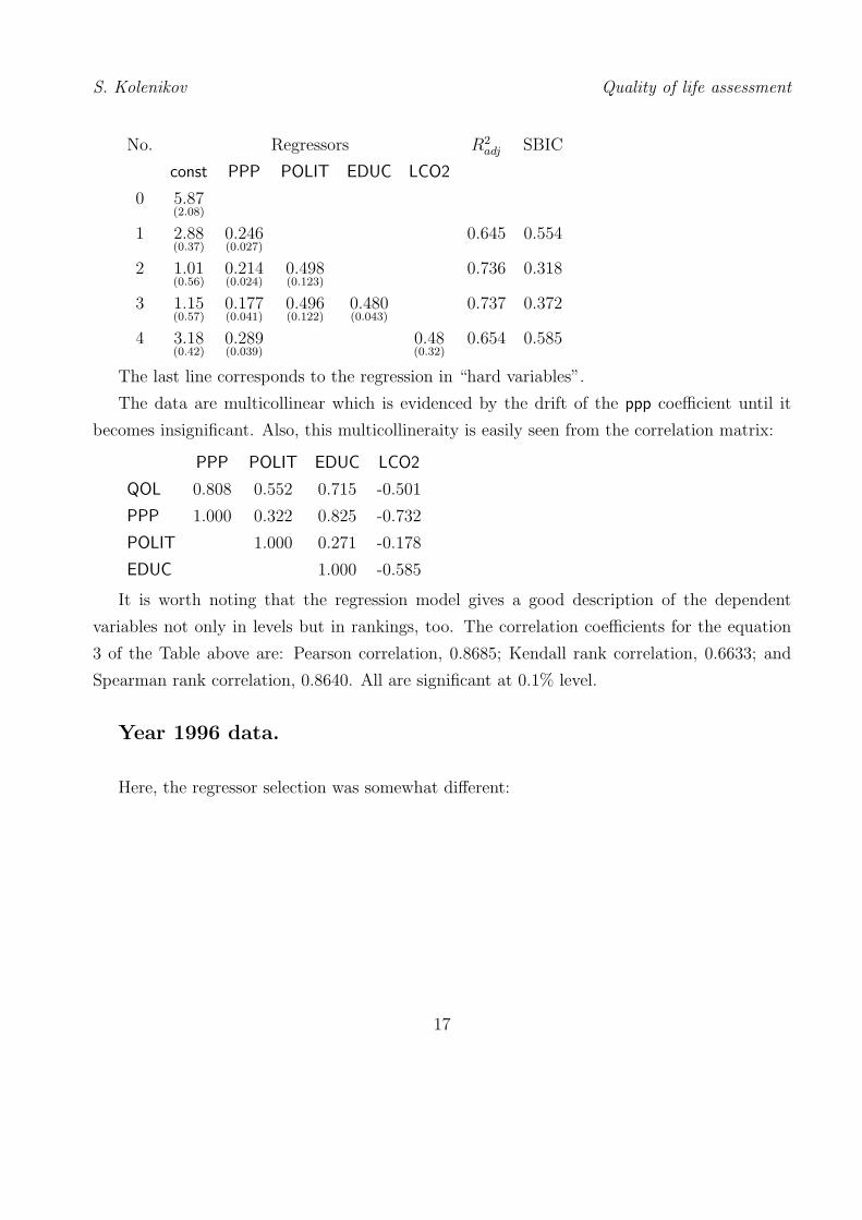
The process of the regressors selection went as follows:
16
S. Kolenikov Quality of life assessment
No. Regressors R2adj SBIC
const PPP POLIT EDUC LCO2
0 5.87(2.08)
1 2.88(0.37)
0.246(0.027)
0.645 0.554
2 1.01(0.56)
0.214(0.024)
0.498(0.123)
0.736 0.318
3 1.15(0.57)
0.177(0.041)
0.496(0.122)
0.480(0.043)
0.737 0.372
4 3.18(0.42)
0.289(0.039)
0.48(0.32)
0.654 0.585
The last line corresponds to the regression in “hard variables”.
The data are multicollinear which is evidenced by the drift of the ppp coefficient until it
becomes insignificant. Also, this multicollineraity is easily seen from the correlation matrix:
PPP POLIT EDUC LCO2
QOL 0.808 0.552 0.715 -0.501
PPP 1.000 0.322 0.825 -0.732
POLIT 1.000 0.271 -0.178
EDUC 1.000 -0.585
It is worth noting that the regression model gives a good description of the dependent
variables not only in levels but in rankings, too. The correlation coefficients for the equation
3 of the Table above are: Pearson correlation, 0.8685; Kendall rank correlation, 0.6633; and
Spearman rank correlation, 0.8640. All are significant at 0.1% level.
Year 1996 data.
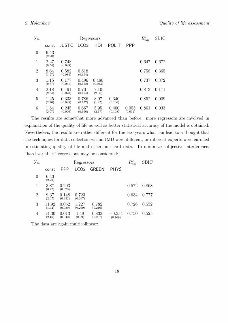
Here, the regressor selection was somewhat different:
17
S. Kolenikov Quality of life assessment
No. Regressors R2adj SBIC
const JUSTC LCO2 HDI POLIT PPP
0 6.43(2.20)
1 2.27(0.54)
0.748(0.089)
0.647 0.672
2 8.64(1.57)
0.582(0.084)
0.818(0.194)
0.758 0.365
3 1.15(0.57)
0.177(0.041)
0.496(0.122)
0.480(0.043)
0.737 0.372
4 2.18(2.34)
0.491(0.078)
0.701(0.174)
7.10(2.08)
0.813 0.171
5 1.25(2.10)
0.333(0.085)
0.786(0.157)
8.07(1.87)
0.340(0.106)
0.852 0.009
6 1.84(2.07)
0.245(0.096)
0.667(0.166)
5.95(2.17)
0.400(0.108)
0.055(0.031)
0.861 0.033
The results are somewhat more advanced than before: more regressors are involved in
explanation of the quality of life as well as better statistical accuracy of the model is obtained.
Nevertheless, the results are rather different for the two years what can lead to a thought that
the techniques for data collection within IMD were different, or different experts were enrolled
in estimating quality of life and other non-hard data. To minimize subjective interference,
“hard variables” regressions may be considered:
No. Regressors R2adj SBIC
const PPP LCO2 GREEN PHYS
0 6.43(2.20)
1 3.87(0.42)
0.203(0.028)
0.572 0.868
2 9.37(2.07)
0.148(0.332)
0.723(0.267)
0.634 0.777
3 11.92(1.92)
0.052(0.039)
1.227(0.269)
0.782(0.216)
0.726 0.552
4 14.30(2.16)
0.013(0.042)
1.49(0.29)
0.833(0.207)
−0.354(0.169)
0.750 0.525
The data are again multicollinear:
18
S. Kolenikov Quality of life assessment
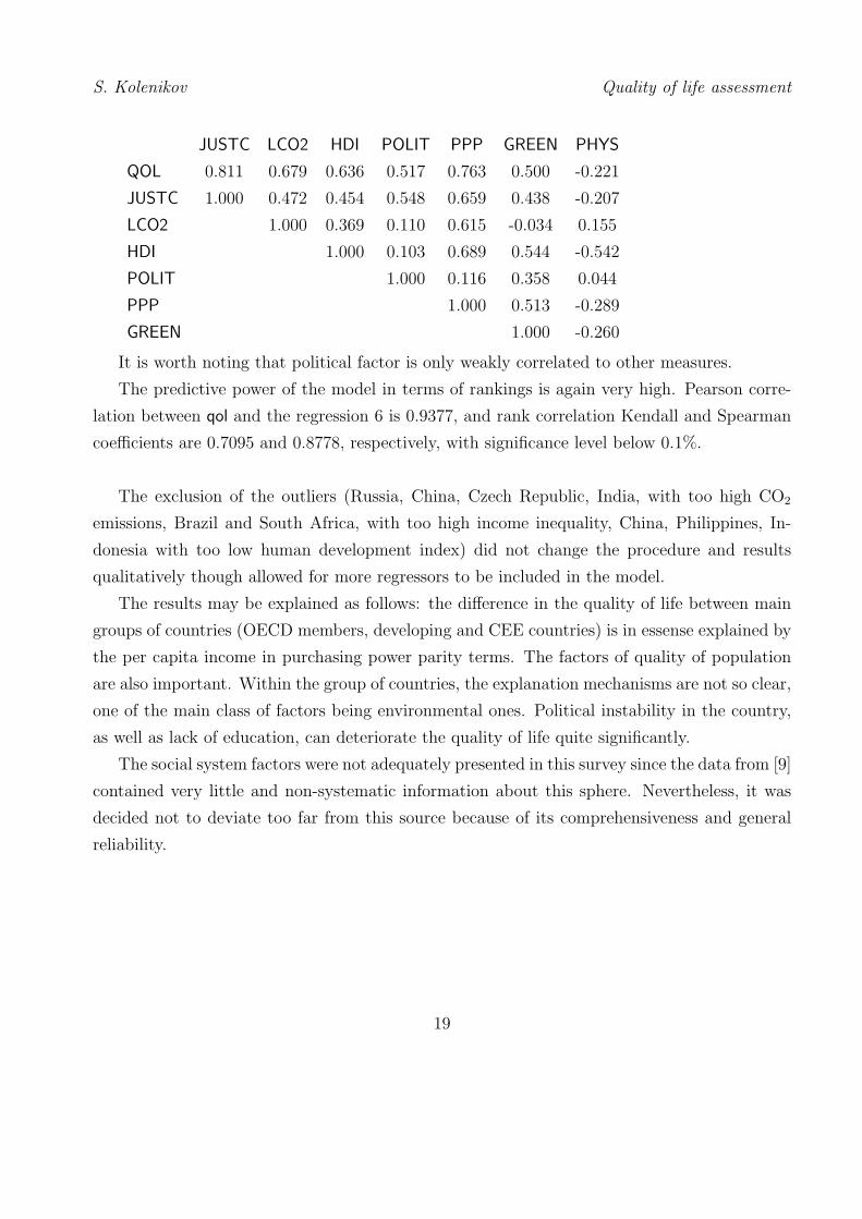
JUSTC LCO2 HDI POLIT PPP GREEN PHYS
QOL 0.811 0.679 0.636 0.517 0.763 0.500 -0.221
JUSTC 1.000 0.472 0.454 0.548 0.659 0.438 -0.207
LCO2 1.000 0.369 0.110 0.615 -0.034 0.155
HDI 1.000 0.103 0.689 0.544 -0.542
POLIT 1.000 0.116 0.358 0.044
PPP 1.000 0.513 -0.289
GREEN 1.000 -0.260
It is worth noting that political factor is only weakly correlated to other measures.
The predictive power of the model in terms of rankings is again very high. Pearson corre-
lation between qol and the regression 6 is 0.9377, and rank correlation Kendall and Spearman
coefficients are 0.7095 and 0.8778, respectively, with significance level below 0.1%.
The exclusion of the outliers (Russia, China, Czech Republic, India, with too high CO2
emissions, Brazil and South Africa, with too high income inequality, China, Philippines, In-
donesia with too low human development index) did not change the procedure and results
qualitatively though allowed for more regressors to be included in the model.
The results may be explained as follows: the difference in the quality of life between main
groups of countries (OECD members, developing and CEE countries) is in essense explained by
the per capita income in purchasing power parity terms. The factors of quality of population
are also important. Within the group of countries, the explanation mechanisms are not so clear,
one of the main class of factors being environmental ones. Political instability in the country,
as well as lack of education, can deteriorate the quality of life quite significantly.
The social system factors were not adequately presented in this survey since the data from [9]
contained very little and non-systematic information about this sphere. Nevertheless, it was
decided not to deviate too far from this source because of its comprehensiveness and general
reliability.
19
S. Kolenikov Quality of life assessment
III.2 Principal Components Analysis
Another approach to reduction of dimensionality is the method of principal components [10]
described in detail in Appendix C.
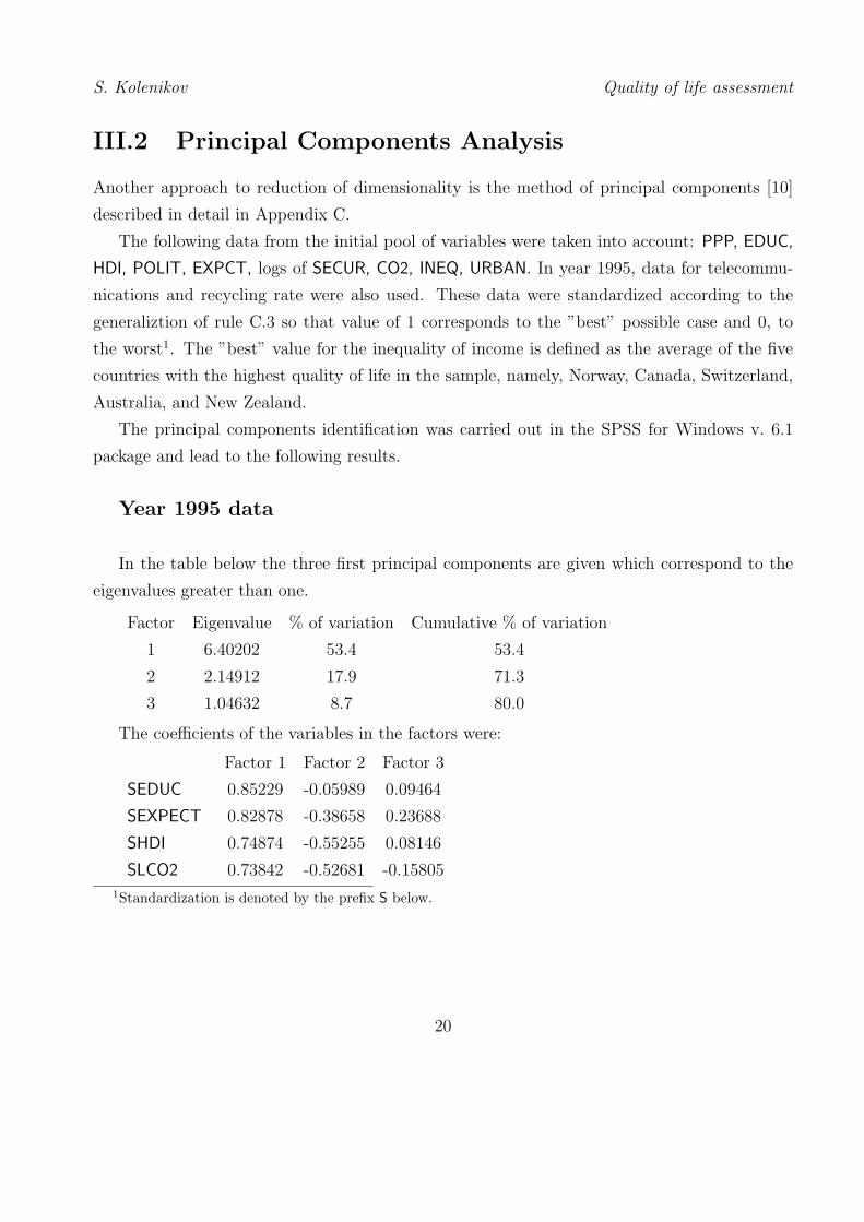
The following data from the initial pool of variables were taken into account: PPP, EDUC,
HDI, POLIT, EXPCT, logs of SECUR, CO2, INEQ, URBAN. In year 1995, data for telecommu-
nications and recycling rate were also used. These data were standardized according to the
generaliztion of rule C.3 so that value of 1 corresponds to the ”best” possible case and 0, to
the worst1. The ”best” value for the inequality of income is defined as the average of the five
countries with the highest quality of life in the sample, namely, Norway, Canada, Switzerland,
Australia, and New Zealand.
The principal components identification was carried out in the SPSS for Windows v. 6.1
package and lead to the following results.
Year 1995 data
In the table below the three first principal components are given which correspond to the
eigenvalues greater than one.
Factor Eigenvalue % of variation Cumulative % of variation
1 6.40202 53.4 53.4
2 2.14912 17.9 71.3
3 1.04632 8.7 80.0
The coefficients of the variables in the factors were:
Factor 1 Factor 2 Factor 3
SEDUC 0.85229 -0.05989 0.09464
SEXPECT 0.82878 -0.38658 0.23688
SHDI 0.74874 -0.55255 0.08146
SLCO2 0.73842 -0.52681 -0.15805
1Standardization is denoted by the prefix S below.
20
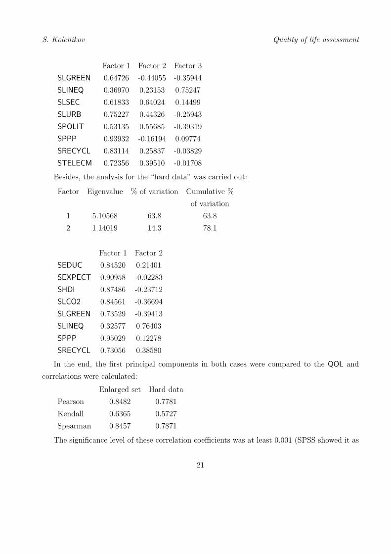
S. Kolenikov Quality of life assessment
Factor 1 Factor 2 Factor 3
SLGREEN 0.64726 -0.44055 -0.35944
SLINEQ 0.36970 0.23153 0.75247
SLSEC 0.61833 0.64024 0.14499
SLURB 0.75227 0.44326 -0.25943
SPOLIT 0.53135 0.55685 -0.39319
SPPP 0.93932 -0.16194 0.09774
SRECYCL 0.83114 0.25837 -0.03829
STELECM 0.72356 0.39510 -0.01708
Besides, the analysis for the “hard data” was carried out:
Factor Eigenvalue % of variation Cumulative %
of variation
1 5.10568 63.8 63.8
2 1.14019 14.3 78.1
Factor 1 Factor 2
SEDUC 0.84520 0.21401
SEXPECT 0.90958 -0.02283
SHDI 0.87486 -0.23712
SLCO2 0.84561 -0.36694
SLGREEN 0.73529 -0.39413
SLINEQ 0.32577 0.76403
SPPP 0.95029 0.12278
SRECYCL 0.73056 0.38580
In the end, the first principal components in both cases were compared to the QOL and
correlations were calculated:
Enlarged set Hard data
Pearson 0.8482 0.7781
Kendall 0.6365 0.5727
Spearman 0.8457 0.7871
The significance level of these correlation coefficients was at least 0.001 (SPSS showed it as
21

S. Kolenikov Quality of life assessment
.000).
The results show a good correlation between rankings as derived from the expert estimate
of the quality of life, on one hand, and the principal components of the available data. Most
variation is explained by the first principal component. The result is almost a striking one. It
implies that quality of life is generally determined by the exogeneous conditions of life given by
“hard variables”.
Year 1996 data
For this year, the results were as follows:
Factor Eigenvalue % of variation Cumulative %
of variation
1 5.24760 52.5 52.5
2 1.41421 14.1 66.6
3 1.26290 12.6 79.2
Factor 1 Factor 2 Factor 3
SEDUC 0.87077 -0.05640 0.17121
SEXPECT 0.90837 -0.23492 0.12007
SHDI 0.77938 -0.49420 -0.04092
SLCO2 0.62766 0.26852 0.45706
SLGREEN 0.62341 -0.48957 -0.45708
SLINEQ 0.44284 0.13045 0.36249
SLSEC 0.67878 0.66243 0.13978
SLURB 0.74948 0.27824 -0.38617
SPOLIT 0.36720 0.50197 -0.70365
SPPP 0.95958 -0.12083 0.06692
It is easily seen that politic environment is least correlated with the first principal component
which supports the statement made earlier (see p. 19) of relatively weak correlation of the
political factor with other variables.
Again, “hard data” based components were determined:
22
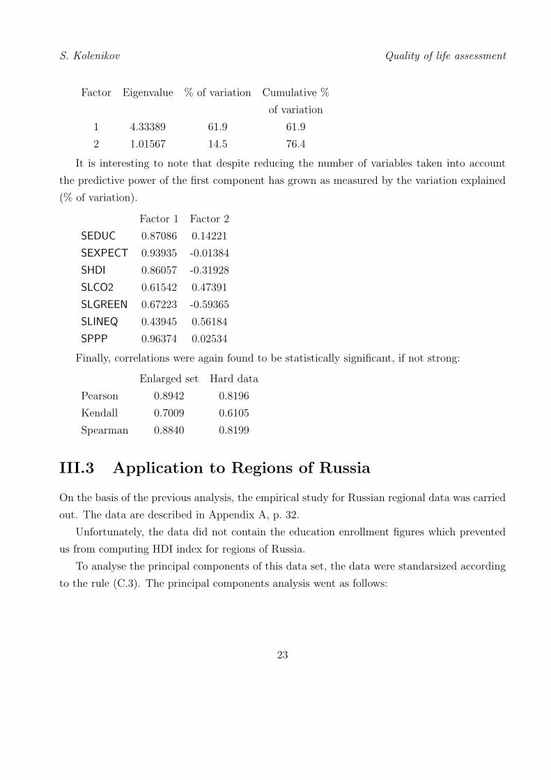
S. Kolenikov Quality of life assessment
Factor Eigenvalue % of variation Cumulative %
of variation
1 4.33389 61.9 61.9
2 1.01567 14.5 76.4
It is interesting to note that despite reducing the number of variables taken into account
the predictive power of the first component has grown as measured by the variation explained
(% of variation).
Factor 1 Factor 2
SEDUC 0.87086 0.14221
SEXPECT 0.93935 -0.01384
SHDI 0.86057 -0.31928
SLCO2 0.61542 0.47391
SLGREEN 0.67223 -0.59365
SLINEQ 0.43945 0.56184
SPPP 0.96374 0.02534
Finally, correlations were again found to be statistically significant, if not strong:
Enlarged set Hard data
Pearson 0.8942 0.8196
Kendall 0.7009 0.6105
Spearman 0.8840 0.8199
III.3 Application to Regions of Russia
On the basis of the previous analysis, the empirical study for Russian regional data was carried
out. The data are described in Appendix A, p. 32.
Unfortunately, the data did not contain the education enrollment figures which prevented
us from computing HDI index for regions of Russia.
To analyse the principal components of this data set, the data were standarsized according
to the rule (C.3). The principal components analysis went as follows:
23

S. Kolenikov Quality of life assessment
Factor Eigenvalue % of variation Cumulative %
of variation
1 4.57974 35.2 35.2
2 2.46205 18.9 54.2
3 1.47313 11.3 65.5
Evidently, the first principal component for Russian data set desribes less variance than that
for international data does. This could be attributed to the great dispersion of main important
characteristics like geographic position, population density, resource base, etc. which can vary
in an order or more of magnitude from say Tambov region to Yakutia.
Even more disappointing were negative correlation between the first component and the
factors in question. It signals that the first component seems to be non-appropriate measure of
quality of life for Russia. As a poet said, ”Russia cannot be measured with a common ruler”.
Factor 1 Factor 2 Factor 3
SCRIME 0.56903 0.29041 -0.56373
SDOC -0.42572 0.48440 0.28692
SDWELL -0.27052 0.76271 0.06008
SEMISSC 0.73695 0.11342 0.57715
SEMISSD 0.69397 0.26316 0.36735
SEXPECT 0.75117 0.32498 -0.40922
SGDP -0.70324 0.14873 -0.38326
SILL 0.51907 -0.11269 0.17854
SMURDER 0.50828 0.64832 -0.30042
SNURSE -0.56748 0.51362 0.27727
SROADS 0.61045 0.48644 -0.01269
STELE -0.62772 0.14088 -0.23013
SUNEMPL -0.54913 0.63101 0.18675
The results could also be in part understood by significantly smaller correlations between the
variables. For instanse, in the correlation matrix of the size 14×14, only 7 correlation coefficients
were greater in absolute values than 0.5 (or 7.7%), while for the international data set, there were
44 of such correlations in 22×22 matrix (19.1%). This less developed multicollinearity increase
estimates efficiency but at the same time might point to less reliable data: they are supposed
24
S. Kolenikov Quality of life assessment
to be more tightly related, and smaller variance could indicate somewhat more stochastic data
generation.
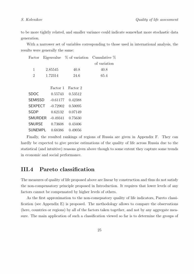
With a narrower set of variables corresponding to those used in international analysis, the
results were generally the same:
Factor Eigenvalue % of variation Cumulative %
of variation
1 2.85545 40.8 40.8
2 1.72314 24.6 65.4
Factor 1 Factor 2
SDOC 0.55743 0.53512
SEMISSD -0.61177 0.42388
SEXPECT -0.72902 0.50095
SGDP 0.62132 0.07149
SMURDER -0.49341 0.75630
SNURSE 0.73608 0.43406
SUNEMPL 0.68386 0.49056
Finally, the resulted rankings of regions of Russia are given in Appendix F. They can
hardly be expected to give precise estimations of the quality of life across Russia due to the
statistical (and intuitive) reasons given above though to some extent they capture some trends
in economic and social performance.
III.4 Pareto classification
The measures of quality of life proposed above are linear by construction and thus do not satisfy
the non-compensatory principle proposed in Introduction. It requires that lower levels of any
factors cannot be compensated by higher levels of others.
As the first approximation to the non-comepsatory quality of life indicators, Pareto classi-
fication (see Appendix E) is proposed. The methodology allows to compare the observations
(here, countries or regions) by all of the factors taken together, and not by any aggregate mea-
sure. The main application of such a classification viewed so far is to determine the groups of
25

S. Kolenikov Quality of life assessment
countries or regions with comparatively higher/lower levels of achievements. This supports an
intuititve idea of existense of clusters with more or less homogeneous quality of life that differ
significantly from that of objects from other clusters. For intracountry region comparison, the
results of classification may serve as a basis for region policy design and conduction.
Pareto classification has been conducted for both international and Russian data sets (all
available data and most relevant factors). For international IMD data, analysis was carried out
for years 1995 and 1996, taking into account the larger set of factors, (sppp, slsec, seduc, slco2,
slurb, sexpect, slineq, shdi, spolit, srecycl, slgreen, stelecm, see data description) as well as factors
selected by the stepwise regressions (see Section III.1).
In year 1995, Pareto classification on the complete set of factors revealed two groups:
1. Argentina, Australia, Austria, Belgium & Luxemburg, Brazil, Canada, Chile, China,
Colombia, Denmark, Egypt, Finland, France, Germany, Greece, Hong Kong, Iceland, In-
dia, Indonesia, Israel, Japan, Jordan, Malaysia, Mexico, Netherlands, New Zealand, Nor-
way, Peru, Portugal, Singapore, Spain, Sweden, Switzerland, Thailand, Turkey, United
Kingdom, USA
2. Czech Republic, Hungary, Ireland, Italy, Korea, Philippines, Russia, South Africa, Tai-
wan, Venezuela
For the narrower set of factors selected by the stepwise regression (ppp, polit, educ, lco2),
there were 5 distinct groups found:
1. Argentina, Austria, Brazil, Chile, Colombia, Denmark, Egypt, Finland, Germany, Hong
Kong, India, Indonesia, Jordan, Malaysia, New Zealand, Norway, Peru, Portugal, Singa-
pore, Spain, Sweden, Switzerland, Thailand, USA
2. Australia, Canada, China, Czech Republic, France, Hungary, Iceland, Ireland, Japan,
Korea, Mexico, Netherlands, Taiwan, Turkey
3. Belgium & Luxemburg, Israel, Italy, United Kingdom, Venezuela
4. Greece, Philippines, South Africa
5. Russia
26
S. Kolenikov Quality of life assessment
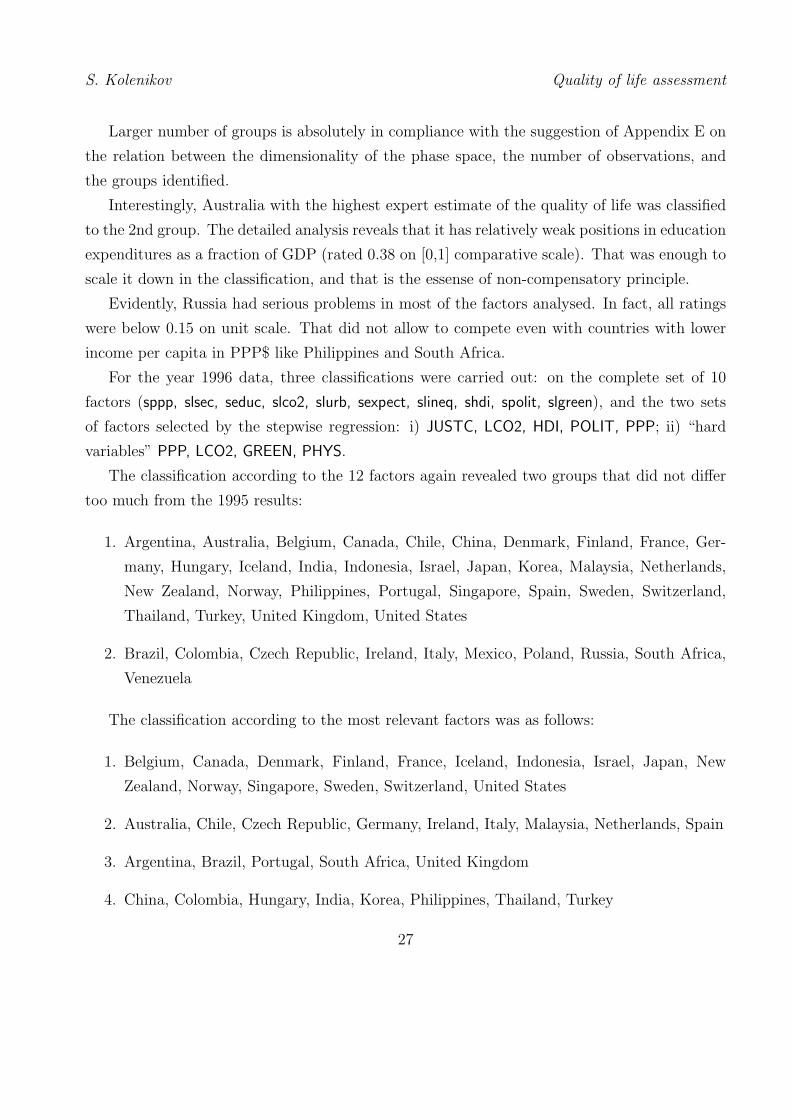
Larger number of groups is absolutely in compliance with the suggestion of Appendix E on
the relation between the dimensionality of the phase space, the number of observations, and
the groups identified.
Interestingly, Australia with the highest expert estimate of the quality of life was classified
to the 2nd group. The detailed analysis reveals that it has relatively weak positions in education
expenditures as a fraction of GDP (rated 0.38 on [0,1] comparative scale). That was enough to
scale it down in the classification, and that is the essense of non-compensatory principle.
Evidently, Russia had serious problems in most of the factors analysed. In fact, all ratings
were below 0.15 on unit scale. That did not allow to compete even with countries with lower
income per capita in PPP$ like Philippines and South Africa.
For the year 1996 data, three classifications were carried out: on the complete set of 10
factors (sppp, slsec, seduc, slco2, slurb, sexpect, slineq, shdi, spolit, slgreen), and the two sets
of factors selected by the stepwise regression: i) JUSTC, LCO2, HDI, POLIT, PPP; ii) “hard
variables” PPP, LCO2, GREEN, PHYS.
The classification according to the 12 factors again revealed two groups that did not differ
too much from the 1995 results:
1. Argentina, Australia, Belgium, Canada, Chile, China, Denmark, Finland, France, Ger-
many, Hungary, Iceland, India, Indonesia, Israel, Japan, Korea, Malaysia, Netherlands,
New Zealand, Norway, Philippines, Portugal, Singapore, Spain, Sweden, Switzerland,
Thailand, Turkey, United Kingdom, United States
2. Brazil, Colombia, Czech Republic, Ireland, Italy, Mexico, Poland, Russia, South Africa,
Venezuela
The classification according to the most relevant factors was as follows:
1. Belgium, Canada, Denmark, Finland, France, Iceland, Indonesia, Israel, Japan, New
Zealand, Norway, Singapore, Sweden, Switzerland, United States
2. Australia, Chile, Czech Republic, Germany, Ireland, Italy, Malaysia, Netherlands, Spain
3. Argentina, Brazil, Portugal, South Africa, United Kingdom
4. China, Colombia, Hungary, India, Korea, Philippines, Thailand, Turkey
27
S. Kolenikov Quality of life assessment
5. Mexico, Poland, Venezuela
6. Russia
The last classification according to the most relevant “hard variables” also was detailed
enough:
1. Argentina, Belgium, Chile, China, Hungary, India, Indonesia, Israel, Italy, Japan, Korea,
Philippines, Portugal, Spain, Sweden, Switzerland, USA
2. Canada, Czech Republic, Denmark, France, Germany, Iceland, Mexico, Norway, Russia,
Turkey, Venezuela
3. Australia, Colombia, Finland, Netherlands, New Zealand, Poland, Singapore, South
Africa, Thailand
4. Brazil, United Kingdom
5. Ireland
6. Malaysia
Relatively high place of Russia (as well as countries like Turkey or Venezuela usually rated
rather low in quality of life estimates) can be explained by subjective factors like political
instability or ideologic barriers still in place. Besides, an expert opinion on these countries may
also be biased by the common fears of “bears in the streets”.
Pareto classification of regions of Russia was also carried out for two sets of factors: the
complete set of data chosen for quality of life analysis, and one-factor-per-factor-group set
(GRP, life expectacny, population per doctor, dwelling per capita, emissions). The resulting
table is given in the Appendix F and by far more successful than the ranking according to the
first principal component.
28
IV. Conclusion
The Quality of Life concept has not yet attracted much attention from the policymakers as
a policy goal to be pursued. Nevertheless, the analysis of the quality of life as a measure of
comparative performance of the society and its evaluation by experts or by the population itself
is of interest. For this analysis, the relation between the quality of life estimations and real
economic variables measured by the official institutions or predicted by macroeconomic models
is to be established.
This Master Thesis attempted to outline the ways of identifying these relations. The hi-
erarchical aggregate quality of life estimate decomposition to the four groups of factors was
proposed. A simple regression analysis of the quality of life in different countries in 1995 on
the factors from these groups was conducted. It was found that the difference in the quality of
life between different countries is well explained by such factors as the GDP per capita in pur-
chasing power parity terms, the level of security in the country, political system adequacy, and
the state of ecology. Each of the groups of hierarchically decomposed factors were represented
by one or two regressors.
Also, principal components of the main indicators of economic and social well-being of a
society were found to be significantly correlated with the expert estimates of the quality of life
and thus may serve as practically implementable method of the quality of life estimation. Such
implementation was done on the Russian regions data.
I am obliged to my scientific advisor Prof. S. A. Aivazian (RAS CEMI) for his guidance and
helpful comments. I am also grateful to V. V. Shakin (Computer Center of RAS) for insighting
communications, and to M. I. Levin (NES, CEMI) and Yu. G. Yepishin (CEMI) for the data
provided.
I claim copyright on all errors and omissions.
29

A. Data
The main source of the data for this research was [9] by International Institute for Manage-
rial Development, Lausanne, which is an institution by World Economic Forum. This book is
published annually and contains the data on more than 40 countries (OECD and other more
or less developed countries, Russia included, sans Gulf region). There is a detailed report on
each of the countries and separate tables for each of the indicators. All factors are collected
into 8 groups: domestic economy, internationalization of economy, government, financial sector,
infrastructure, management, science, people. The data and the very indicators tend to differ
from year to year, so that no common reference to the Table’s numbers is possible, but never-
theless the most important data fortunately did enter the book in all year analysed under the
same name1. There are both real data (“hard variables”) and expert estimation on the (0,10)
scale where 0 corresponds to the lowest imaginable level, and 10, to the best one.
There is an expert estimation of the quality of life (Table 8.33 in [9], 1996) which was
extensively used in this study for empirical tests. Some other data were considered relevant to
the quality of life analysis and used in multivariate analysis and modelling as described below:
QOL Quality of life, an expert estimation on (0,10) scale; 10 for adequate quality of life, 0 for
inadequate.
Welfare factors group:
PPP Gross domestic product per capita (US$ at current prices and purchasing power parity)
GDP Gross domestic product at constant prices (US $ billions at current prices)
INEQ Inequality of income distribution, the ratio of the wealthiest 20% of population income
to that of the 20% poorest
1It might be suspected that the methodology of data collection did change from year to year as some
descriptive statistics evidenced.
30
S. Kolenikov Quality of life assessment
INFL Inflation, % per year
URBAN Urbaniztion influence, expert estimate: 0, cities drain national resources; 10, cities sup-
port national development
Quality of population group:
EXPCT Life expectancy at birth, years
UNEMPL Unemployment, % of labor force
ILLIT Adult (over 15) illiteracy rate, % of population
HDI Human development index, Section II.2
JUSTC Expert estimation of justice in country; 10 for adequate justice system, 0 for inadequate
CRIME Serious crime: number of murders, violent crimes or armed robberies reported per 100
th. inhabitants
SECUR Security in the country, expert estimation: 0, no confidence among people that their
person and property is protected; 10, full confidence
COMPT Attitude towards competitivenes, expert estimation: 0, values of the society do not sup-
port competitiveness (such as pursuing individual interest at the expense of company
interest); 10, support competitiveness (such as hard work, tenacity or loyalty)
POLIT Political system, expert estimation: 0, needs serious restructuring; 10, is well up-to-date
for todays economic challenges
TAXES Personal taxes influence, expert estimate: 0, discourage individual work initiative; 10,
encourage individual work initiative
Quality of environment:
CO2 CO2 emissions from industrial processes in metric tons per capita
GREEN Greenhouse index, carbon heating equivalents in metric tons per capita
Social system adequacy:
31

S. Kolenikov Quality of life assessment
CONTR Contribution to the social security funds, the sum of employee’s and employer’s contri-
bution, % GDP
EDUC Education expenditures, % GDP
PHYS Population per physician
NURSE Population per nurse
Some of the indicators may be considered as applicable to more than one group. E. g.,
URBAN may be placed into environmental group, etc.
The set of the data used for the analysis is available on the Internet on the NES site.
http://www.nes.cemi.rssi.ru/∼skolenik/qol/mthesis/comp9596.xls
Data for Russia were taken from the official issue of GOSKOMSTAT (State Committee
for Statistics of Russian Federation) [22]. This two-volumed book contains a comprehensive
set of official statistical data for 81 regions of Russia, including data for national autonomies,
if necessary and available. These data were collected from statistical agencies which in turn
achieve them from enterprises and instiutions as well as by censuses and surveys; from Russian
ministries and governmental organizations, and from the third party agencies conducting sur-
veys and analyses of economic and social issues. Most data are dated by year 1995; there is
also (preliminary) data for year 1996.
From about 250 statistical tables, the following data were used for the analysis:
GDP GDP per capita, th. rb.
EXPECT Life expectancy at birth, years
UNEMPL Unemployment rate, %
ILL Illness rate, newly diagnosed per 1000 population
DOC Population per physician
NURSE Population per nurse
DWELL Dwelling per capita, sq. m.
32
S. Kolenikov Quality of life assessment
CRIME Registered crimes per 100000 of population
MURDER Murders per 100000 of population
EMISSC CO2 emissions, tons per capita
EMISSD CO2 emissions, tons per $ 1000 of GDP
TELE Telecommunication services, rbs. per capita
ROADS Density of motorways, km/sq. km
These data are also available on the Internet via
http://www.nes.cemi.rssi.ru/∼skolenik/qol/mthesis/rrus.xls
33
B. Stepwise regression
The method of stepwise regression is used to identify a regression model, or, equivalently, to
select the most appropriate variables to explain the dependent one. At the first step, the regres-
sor with the highest correlation with the dependent variable was selected to be included in the
model. On the following steps, the variable is chosen which explains the greatest part of varia-
tion of the residual from the previous step regression as signalled by the partial correlation with
fixed other variables (already selected at the earlier steps), or correlation between the residual
and the considered variables from a pool of regressors. Let us denote y, the dependent variable;
x1, . . . , xk, the regressors chosen on earlier k steps; x(k)k+1, . . . , x
(k)n , the pool of regressors. Then
the process goes as follows:
1. Calculate the residuals ε of the explaining regression:
y = a(k)1 x1 + . . .+ a
(k)k xk + ε(k) (B.1)
2. Find the correlation coefficients of ε(k) and x(k)i , i = k + 1, . . . , n.
3. Choose the regressors with the greatest correlation:
xk+1 = Arg maxj
corr(ε(k), x(k)j ), j = k + 1, . . . , n (B.2)
The process terminates when the regressor chosen is not significant. There may also be
other measures for model identification, e. g., Shwartz Bayesian information criteria (SBIC)
which shows the trade-off between the model accuracy and the number of regressors, or R2adj.
34

C. Principal components
The principal components method1 is used to reduce the dimensionality of the set of statistically
processed data, e. g., for visual purposes or in order to obtain a low-dimension model. In this
reduction, from the initial set of data x(1)i , . . . , x
(p)i , i = 1, . . . , n, where p is the number of
indicators, and n, number of observations, a new set of variables z(1), . . . , z(p′), p′ < p (or even
p′ � p) is obtained as an Arg max Ip′(Z(X)) for some information measure Ip′(·).If one is looking for the set z(1), . . . , z(p′) allowing only for linear transformations of the x’s
and maximizing the explained variance of the x’s
Ip′(Z(X)) =Var z(1) + . . .+ Var z(p′)
Varx(1) + . . .+ Varx(p)(C.1)
then the resulting z’s are called principal components, i. e., the factors that change most while
switching between observations.
Principal components are used to restore the values of the variables from the least possible
information set. For instance, the principal components of one’s body may be inferred from
the usually measured height, waist, neck size, etc., which are used to select a dress or a suit.
Nevertheless often this information is redundant since these characteristic are to some extent
interrelated: one seldom has short legs if he is 6 feet 5 inches tall. The idea of reduction of such
redundancy is exploited in the principal components method. Sometimes, one figure is enough
to identify the whole variety of the data if the scatter diagram has the only vividly evident axis.
Principal components depend only on the variance-covariance matrix Varx so they are
invariant with respect to linear shift of variables x(j) → x(j) − c(j) ∀ c(j). Further we shall
assume that the data are centered: E x(j) = 0.
It can be shown that principal components may be found as eigenvectors of the variance-
covariance matrix. The first principal components (i. e., the linear combination which explains
1 The description follows [10]
35
S. Kolenikov Quality of life assessment
the major part of variance in the set of x’s) corresponds to the largest eigenvalue of the variance-
covariance matrix. Other components correspond to the consequently decreasing eigenvalues.
The use of the principal components method is quite natural when all components of the X
vector are of the same nature and are expressed in the same units. If they are not, the result
would depend heavily on the scale of the variables. Hence it makes sense to standardize them.
Two normalization are generally used:
x∗(j) =x(j) − E x(j)
√Varx(j)
(C.2)
x∗∗(j) =x(j) −minx(j)
maxx(j) −minx(j)(C.3)
The transformation (C.2) leads to the set of variables with zero mean and unit variance,
while the transformation (C.3) reduces all variables to the [0,1] range.
36

D. Rank correlation
The concept of rank correlation1 appears in the analysis of statistical relationship between or-
dinal variables, e. g., ranks of other variables or rank of objects derived by expert estimation,
which show the degree of maturity of the analysed characteristic. It is useful when the quan-
titative measure of the characteristic is not available or has only a relative sense as a tool for
further ranking. It is also useful as a robust measure of interdependence of the two variables
(though the concept of rank correlation can be generalized to the multivariate case).
Hence, the object of the analysis are labels indicating the rank x(k)i of the object i in the
total range of objects (i = 1, . . . , n) by the k-th characteristic, (k = 0, . . . , p).
The specific feature of an ordinal random variable is varying domain of possible values:
the length of the range is determined by the very sample size and necessarily grows with it
(while for cardinal random variables, the distribution is usually supposed to be the same for
all cases). Another difficulty may be coinciding ranges, i. e., when the two objects display the
characteristic to the same degree. In this case, fractional ranges are used.
The following zero hypothesis is usually formulated:
H0 :
a) random variables{xk}k=0,p are statistically independent
b) all elementary outcomes are equiprobable, p =1
n!
(D.1)
There are two popular numerical measures of rank correlation, Spearman coefficient and
Kendall coefficient. The former was proposed in 1904 by C. Spearman:
τ(S)kj = 1− 6
n3 − n∑i=1
n(x
(k)i − x
(j)i
)2
(D.2)
If the two rankings coincide, τ(S)kj = 1, and when they are opposite, τ
(S)kj = −1. In all other
cases, |τ (S)kj | < 1. The formula (D.2) may be generalized to the case of coinciding ranges.
1 The description follows [11]
37
S. Kolenikov Quality of life assessment
The other measure of rank correlation is Kendall coefficient:
τ(K)kj = 1− 4ν(X(k), X(j))
n(n− 1)(D.3)
where ν(X(k), X(j)) is the number of neighbor trades of the X(j) sequence necessary to obtain
X(k) sequence, or, equivalently, the number of inversions i. e., pairs of sequences elements placed
in different order. Again, if the two rankings coincide, τ(K)kj = 1, and when they are opposite,
τ(K)kj = −1; in all other cases, |τ (K)
kj | < 1.
Determining Kendall coefficient is more computationally intensive than that of Spearman
index, but the statistical properties of the former are developed to a greater extent. Moreover,
it is more convenient as new observations are added to the sample.
Both of the coefficients may be generalized in the following way. For any bivariate system
of n observations (X(k)T
X(j)T
)=
(x
(k)1 , . . . , x
(k)n
x(j)1 , . . . , x
(j)n
)(D.4)
define a rule mapping each pair (x(l)i1, x
(l)i2
) a number (“label”) a(l)i1i2
, this rule being negatively
symmetric (a(l)i1i2
= −a(l)i2i1
) and centric (a(l)ii = 0 ∀l = k, j ∀i = 1, . . . , n). Then a generalized
rank correlation coefficient r(g) may be defined as
r(g)kj =
∑ni1=1
∑ni2=1 a
(k)i1i2a
(j)i1i2√∑n
i1=1
∑ni2=1 a
(k)i1i2
2·∑n
i1=1
∑ni2=1 a
(j)i1i2
2(D.5)
The two previously defined correlation coefficients can be expressed in terms of this generalized
correlation coefficient as follows: by putting a(l)i1i2
= x(l)i1− x(l)
i2, l = k, j, one obtains usual corre-
lation coefficient if x(l)i is a value of l-th variable in i-th observation, and Spearman correlation
coefficient τ(S)kj , if x
(l)i is the rank of i-th object in the l-th related ranking; and by putting
a(l)i1i2
= sign (x(l)i2− x(l)
i1), one obtains formula for Kendall correlation coefficient (D.3). Thus the
two coefficients are closely related though Spearman coefficient gives greater weights for more
distant pairs, for n ≥ 10 and τ(S)kj , τ
(K)kj not close to 1 the approximation being
τ(S)kj ≈ 1, 5 τ
(K)kj
.
38
S. Kolenikov Quality of life assessment
Testing hypothesis of correlation significance is carried out for relatively large samples (n ≥10) for given significance level α via inequalities
|τ (S)| > tα/2(n− 2)
√1− (τ (S))2
n− 2(D.6)
|τ (K)| > uα/2
√2(2n+ 5)
9n(n− 1)(D.7)
where tq(ν) and uq is a 100%q percentile points of Student with ν d. f., and normal distributions.
If the inequalities (D.6) and (D.7) hold, H0 needs to be rejected.
39
E. Pareto classification
The idea of Pareto classification extends the Pareto relation, or dominance, determined for the
two multidimensional objects, to the case of m > 2 objects. This approach was proposed by
V. V. Shakin [21].
The p-th n-dimensional object, or observation, x(p) = (x(p)1 , . . . , x
(p)n ) is said to weakly
Pareto-dominate q-th object x(q), p 6= q, q ∈ {1, . . . ,m} (denote this as x(p) � x(q)) if for
all k = 1, . . . , n, x(p)k ≥ x
(q)k . Another popular notion is that x(p) is a weak Pareto improve-
ment of x(q). Pareto dominance (improvement) is called strict (or simply Pareto dominance) if,
besides, there exists l ∈ {1, . . . , n} such that x(p)l > x
(q)l . Then we denote this as x(p) � x(q).
The algorithm of Pareto classification determines consequently Pareto boundaries of the su-
perior (majorant) objects, as compared to all the others. The first layer consists of observations
X(1) = {x(p)|p ∈ I1}, I1 ⊂ {1, . . . , n} such that there are no objects ”better”, in Pareto sense,
i. e., in all respects, than x(p) from the first Pareto layer X(1): ∀ q 6= p, q = 1, . . . ,m x(q) 6� x(p).
This is a set of Pareto optimal points: for neither of them the situation can be improved in
any factors without making some other factors worse. When all such objects are determined,
the process recursively continues for the sample with elements from X(1) thrown out until all
objects are given their respective class numbers: x(p) ∈ X(2) ⇔ ∀x(q) � x(p) x(q) ∈ X(1),
x(p) ∈ X(3) ⇔ ∀x(q) � x(p) x(q) ∈ X(1) ∪X(2), etc.
If for all p the components of the n-dimensional vector x(p) are perfectly correlated (or if
the objects are characterized by the only one dimension), this procedure will find m classes
I1, . . . , Im. On the other hand, if the dimensionality of vectors being compared is too large
(greater than the very number of objects), and the components are not correlated (or only
weakly correlated), it is likely that all objects would belong to the same (first) Pareto class.
The process of classification may go in the other direction, namely, selecting the ”worst”
objects first. This procedure will result in a different classification, with different allocation
of objects among classes and, possibly, different number of classes. These two ways can be
40
S. Kolenikov Quality of life assessment
reciprocated by simply negating the components of vectors x(p). It can be directly shown that
objects with extreme realizations of the factors (∃ k, l | x(p)k = 1, x
(p)l = 0 in our normalization)
will fall into the first class in both classifications.
The main advantages of this approach as compared to the regression and principal com-
ponents methods described above is its non-compensatory property. Besides, this method is
scale-independent; in fact, it suffices to provide rankings of the objects to build Pareto classifi-
cation.
The non-compensatory principle, as described in Chapter I, postulates impossibility to
compensate deterioration in one of the indicators, or components, by improvements in others.
In fact, this ”transfer” makes the two states of Nature (the initial one and the perturbed one)
Pareto uncomparable: neither of them will constitute Pareto improvement over the other.
41
F. Rankings of Regions of Russia
The principal components analysis (see Section III.3) and Pareto-classification (see Section III.4)
of data for the regions of Russian Federation were carried out. There were two sets of variables
used in principal components indentification: a broader one with 14 variables, and a narrower
one with 7 variables similar to those used in international quality of life comparisons. The
corresponding rankings are given in columns 2 and 3 of the table below. For Pareto rankings,
the same set of 14 variables was used (column 4) as well as a set of factors selected by one from
each of the main groups outlined in Introduction: GRP per capita, life expectacny at birth,
population per doctor, dwelling per capita, and emissions.
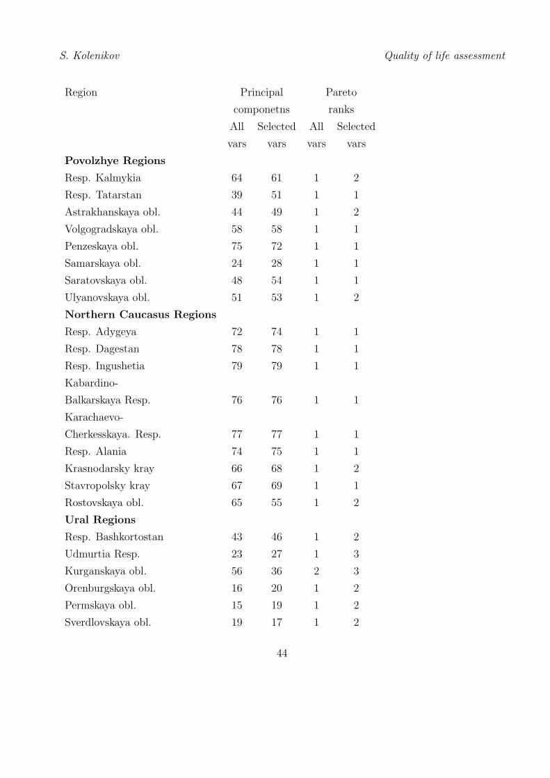
Region Principal Pareto
components ranks
All Selected All Selected
vars vars vars vars
Northern Regions
Resp. Karelia 12 12 1 2
Resp. Komi 4 2 1 2
Arkhangelskaya obl. 18 15 1 2
Vologdskaya obl. 17 13 1 1
Murmanskaya obl. 14 9 1 2
North-Western Regions
St. Peterburg, city 32 30 1 1
Leningradskaya obl. 53 37 1 1
Novgorodskaya obl. 34 34 1 2
Pskovskaya obl. 59 52 1 1
42
S. Kolenikov Quality of life assessment
Region Principal Pareto
componetns ranks
All Selected All Selected
vars vars vars vars
Central Regions
Bryanskaya obl. 71 65 1 2
Vladimirskaya obl. 70 66 1 2
Ivanovskaya obl. 37 50 1 2
Kaluzhskaya obl. 57 59 1 2
Kostromskaya obl. 50 48 1 2
Moscow, city 11 23 1 1
Moscovskaya obl. 69 73 1 2
Orlovskaya obl. 62 63 1 2
Ryazanskaya obl. 20 33 1 1
Smolenskaya obl. 35 45 1 1
Tverskaya obl. 38 41 1 1
Tul’skaya obl. 29 38 1 3
Yaroslavskaya obl. 31 32 1 1
Volga–Vyatka Regions
Resp. Mary El 68 56 1 3
Resp. Mordovia 54 60 1 1
Resp. Chuvashia 60 64 1 2
Kirovskaya obl. 41 44 1 3
Nizhegorodskaya obl. 47 47 1 2
Central Chernozemye Regions
Belgorodskaya obl. 61 67 1 1
Voronezhskaya obl. 63 71 1 1
Kurskaya obl. 55 62 1 1
Lipetskaya obl. 26 35 1 1
Tambovskaya obl. 73 70 1 2
43
S. Kolenikov Quality of life assessment
Region Principal Pareto
componetns ranks
All Selected All Selected
vars vars vars vars
Povolzhye Regions
Resp. Kalmykia 64 61 1 2
Resp. Tatarstan 39 51 1 1
Astrakhanskaya obl. 44 49 1 2
Volgogradskaya obl. 58 58 1 1
Penzeskaya obl. 75 72 1 1
Samarskaya obl. 24 28 1 1
Saratovskaya obl. 48 54 1 1
Ulyanovskaya obl. 51 53 1 2
Northern Caucasus Regions
Resp. Adygeya 72 74 1 1
Resp. Dagestan 78 78 1 1
Resp. Ingushetia 79 79 1 1
Kabardino-
Balkarskaya Resp. 76 76 1 1
Karachaevo-
Cherkesskaya. Resp. 77 77 1 1
Resp. Alania 74 75 1 1
Krasnodarsky kray 66 68 1 2
Stavropolsky kray 67 69 1 1
Rostovskaya obl. 65 55 1 2
Ural Regions
Resp. Bashkortostan 43 46 1 2
Udmurtia Resp. 23 27 1 3
Kurganskaya obl. 56 36 2 3
Orenburgskaya obl. 16 20 1 2
Permskaya obl. 15 19 1 2
Sverdlovskaya obl. 19 17 1 2
44
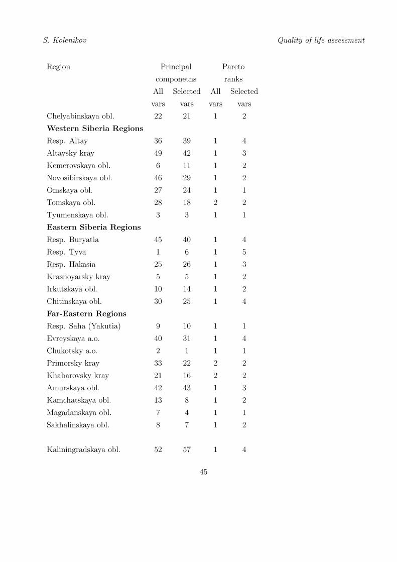
S. Kolenikov Quality of life assessment
Region Principal Pareto
componetns ranks
All Selected All Selected
vars vars vars vars
Chelyabinskaya obl. 22 21 1 2
Western Siberia Regions
Resp. Altay 36 39 1 4
Altaysky kray 49 42 1 3
Kemerovskaya obl. 6 11 1 2
Novosibirskaya obl. 46 29 1 2
Omskaya obl. 27 24 1 1
Tomskaya obl. 28 18 2 2
Tyumenskaya obl. 3 3 1 1
Eastern Siberia Regions
Resp. Buryatia 45 40 1 4
Resp. Tyva 1 6 1 5
Resp. Hakasia 25 26 1 3
Krasnoyarsky kray 5 5 1 2
Irkutskaya obl. 10 14 1 2
Chitinskaya obl. 30 25 1 4
Far-Eastern Regions
Resp. Saha (Yakutia) 9 10 1 1
Evreyskaya a.o. 40 31 1 4
Chukotsky a.o. 2 1 1 1
Primorsky kray 33 22 2 2
Khabarovsky kray 21 16 2 2
Amurskaya obl. 42 43 1 3
Kamchatskaya obl. 13 8 1 2
Magadanskaya obl. 7 4 1 1
Sakhalinskaya obl. 8 7 1 2
Kaliningradskaya obl. 52 57 1 4
45
Bibliography
[1] Frank M. Andrews, Stephen B. Whitney. Social indicators of well-being. Plenum Press,
New York, 1976.
[2] A. Bowling. Measuring Health. Open University Press, 1991.
[3] Health in your life. Questionaire. RAS, Institute of Sociology, St. Peterburg branch, 1998.
In Russian.
[4] Russian Longitudinal Monitoring Survey. Round VI. University of North Carolina, Chapel
Hill, 1997.
[5] The final report on The system of statistical indicators of the quality of life of population.
RAS CEMI, 1997. In Russian.
[6] Herman Haken. Advanced Synergetics. Springer-Verlag, 1983.
[7] L. I. Polischuk. Multicriteria economic and mathematical models analysis. Nauka, Novosi-
birsk, 1989. In Russian.
[8] A. V. Petrov. Information technologies in social and economic growth management. Re-
port at scientific and practical workshop at Russian Federation President Administration.
Moscow, 1997.
[9] The World Competetiveness Yearbook. Institute for Mangerial Development, Lausanne,
1996.
[10] S. A. Aivaizian, V. M. Buchstaber, I .S. Yenyukov, L. D. Meshalkin. Applied Statistics.
Classification and Reduction of Dimensionality. Moscow, 1989.
46
S. Kolenikov Quality of life assessment
[11] S. A. Aivaizian, I .S. Yenyukov, L. D. Meshalkin. Applied Statistics. Study of Relationships.
Moscow, 1985.
[12] W. H. Greene. Econometric Analysis. 2nd edition. New York, McMillan, 1993.
[13] Angus Campbell, Philip E. Converse, Willard L. Rodgers. The quality of American life,
Russell sage foundation, New York, 1976.
[14] D. C. Shin and D. M. Johnson. Avowed happiness as an overall assessment of the quality
of life. Social Indicators Research, 5, 1978, 475–492.
[15] R. Veenhoven et al. Data-Book of Happiness. Reidel, 1984.
[16] R. Veenhoven et al. Bibliography of Happiness. Erasmus University of Rotterdam, 1993.
[17] Quality of Life: Problems of Assessment and Measurement. UNESCO, Paris, 1983.
[18] Human Development in Russian Federation Report. Moscow, Academy, 1995. In Russian.
[19] Human Development Report. UNDP, New York, Oxford, 1993, 1995, 1996.
[20] Anthony B. Atkinson. On the Measurement of Inequality, J. of Ec. Theory, 2, 1970, 244–
263.
[21] Shakin V. V. Pareto classification of the Finite Sample Sets, Applications of Multivariate
Statistical Analysis in Economics and Assessment of Production Quality. Proceedings of
V Scientific Conference of CIS States. RAS CEMI, 1993. In Russian.
[22] Regions of Russia. State Committee for Statistics of Russian Federation. Moscow, 1997.
[23] Zen and the Art of Motorcycle Maintenance. Robert M. Pirsig, Transworld Publishers,
1978.
47