High-density genotyping: an overkill for QTL mapping? Lessons

learned from a case study in maize and simulations

Michael Stange, H. Friedrich Utz, Tobias A. Schrag, Albrecht E. Melchinger, Tobias

Würschum

M. Stange, H. F. Utz, T. A. Schrag, A. E. Melchinger, Institute of Plant Breeding, Seed

Science, and Population Genetics, University of Hohenheim, 70599 Stuttgart, Germany

T. Würschum (), State Plant Breeding Institute, University of Hohenheim, 70599 Stuttgart,

Germany

Email: tobias.wuerschum@uni-hohenheim.de

Supplementary Information

2

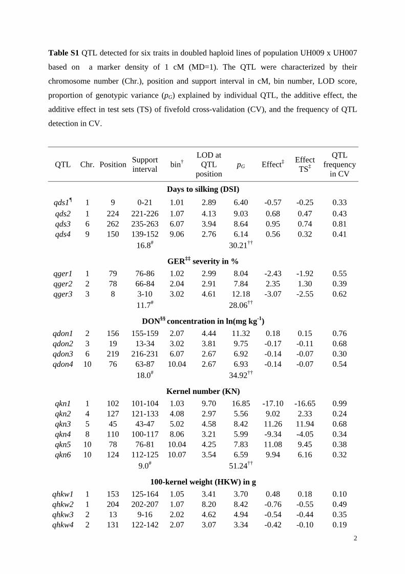
Table S1 QTL detected for six traits in doubled haploid lines of population UH009 x UH007

based on a marker density of 1 cM (MD=1). The QTL were characterized by their

chromosome number (Chr.), position and support interval in cM, bin number, LOD score,

proportion of genotypic variance (pG) explained by individual QTL, the additive effect, the

additive effect in test sets (TS) of fivefold cross-validation (CV), and the frequency of QTL

detection in CV.

QTL Chr. Position Support interval

bin† LOD at

QTL position

pG Effect‡ Effect TS‡

QTL frequency

in CV

Days to silking (DSI)

qds1¶ 1 9 0-21 1.01 2.89 6.40 -0.57 -0.25 0.33 qds2 1 224 221-226 1.07 4.13 9.03 0.68 0.47 0.43 qds3 6 262 235-263 6.07 3.94 8.64 0.95 0.74 0.81 qds4 9 150 139-152 9.06 2.76 6.14 0.56 0.32 0.41

16.8# 30.21††

GER‡‡ severity in %

qger1 1 79 76-86 1.02 2.99 8.04 -2.43 -1.92 0.55 qger2 2 78 66-84 2.04 2.91 7.84 2.35 1.30 0.39 qger3 3 8 3-10 3.02 4.61 12.18 -3.07 -2.55 0.62

11.7# 28.06††

DON§§ concentration in ln(mg kg-1)

qdon1 2 156 155-159 2.07 4.44 11.32 0.18 0.15 0.76 qdon2 3 19 13-34 3.02 3.81 9.75 -0.17 -0.11 0.68 qdon3 6 219 216-231 6.07 2.67 6.92 -0.14 -0.07 0.30 qdon4 10 76 63-87 10.04 2.67 6.93 -0.14 -0.07 0.54

18.0# 34.92††

Kernel number (KN)

qkn1 1 102 101-104 1.03 9.70 16.85 -17.10 -16.65 0.99 qkn2 4 127 121-133 4.08 2.97 5.56 9.02 2.33 0.24 qkn3 5 45 43-47 5.02 4.58 8.42 11.26 11.94 0.68 qkn4 8 110 100-117 8.06 3.21 5.99 -9.34 -4.05 0.34 qkn5 10 78 76-81 10.04 4.25 7.83 11.08 9.45 0.38 qkn6 10 124 112-125 10.07 3.54 6.59 9.94 6.16 0.32

9.0# 51.24††

100-kernel weight (HKW) in g

qhkw1 1 153 125-164 1.05 3.41 3.70 0.48 0.18 0.10 qhkw2 1 204 202-207 1.07 8.20 8.42 -0.76 -0.55 0.49 qhkw3 2 13 9-16 2.02 4.62 4.94 -0.54 -0.44 0.35 qhkw4 2 131 122-142 2.07 3.07 3.34 -0.42 -0.10 0.19

3

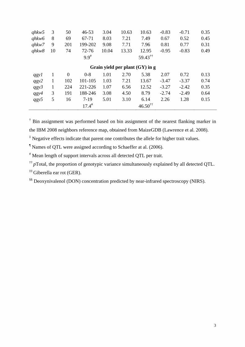
qhkw5 3 50 46-53 3.04 10.63 10.63 -0.83 -0.71 0.35 qhkw6 8 69 67-71 8.03 7.21 7.49 0.67 0.52 0.45 qhkw7 9 201 199-202 9.08 7.71 7.96 0.81 0.77 0.31 qhkw8 10 74 72-76 10.04 13.33 12.95 -0.95 -0.83 0.49

9.9# 59.43††

Grain yield per plant (GY) in g

qgy1 1 0 0-8 1.01 2.70 5.38 2.07 0.72 0.13 qgy2 1 102 101-105 1.03 7.21 13.67 -3.47 -3.37 0.74 qgy3 1 224 221-226 1.07 6.56 12.52 -3.27 -2.42 0.35 qgy4 3 191 188-246 3.08 4.50 8.79 -2.74 -2.49 0.64 qgy5 5 16 7-19 5.01 3.10 6.14 2.26 1.28 0.15

17.4# 46.50†† † Bin assignment was performed based on bin assignment of the nearest flanking marker in

the IBM 2008 neighbors reference map, obtained from MaizeGDB (Lawrence et al. 2008). ‡ Negative effects indicate that parent one contributes the allele for higher trait values. ¶ Names of QTL were assigned according to Schaeffer at al. (2006). # Mean length of support intervals across all detected QTL per trait. †† pTotal, the proportion of genotypic variance simultaneously explained by all detected QTL. ‡‡ Giberella ear rot (GER). §§ Deoxynivalenol (DON) concentration predicted by near-infrared spectroscopy (NIRS).

4

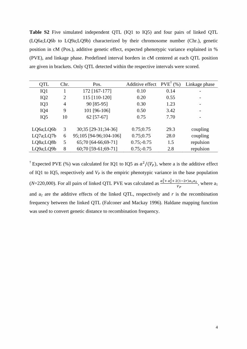
Table S2 Five simulated independent QTL (IQ1 to IQ5) and four pairs of linked QTL

(LQ6a;LQ6b to LQ9a;LQ9b) characterized by their chromosome number (Chr.), genetic

position in cM (Pos.), additive genetic effect, expected phenotypic variance explained in %

(PVE), and linkage phase. Predefined interval borders in cM centered at each QTL position

are given in brackets. Only QTL detected within the respective intervals were scored.

QTL Chr. Pos. Additive effect PVE† (%) Linkage phase IQ1 1 172 [167-177] 0.10 0.14 - IQ2 2 115 [110-120] 0.20 0.55 - IQ3 4 90 [85-95] 0.30 1.23 - IQ4 9 101 [96-106] 0.50 3.42 - IQ5 10 62 [57-67] 0.75 7.70 -

LQ6a;LQ6b 3 30;35 [29-31;34-36] 0.75;0.75 29.3 coupling LQ7a;LQ7b 6 95;105 [94-96;104-106] 0.75;0.75 28.0 coupling LQ8a;LQ8b 5 65;70 [64-66;69-71] 0.75;-0.75 1.5 repulsion LQ9a;LQ9b 8 60;70 [59-61;69-71] 0.75;-0.75 2.8 repulsion

† Expected PVE (%) was calculated for IQ1 to IQ5 as / , where a is the additive effect

of IQ1 to IQ5, respectively and VP is the empiric phenotypic variance in the base population

(N=220,000). For all pairs of linked QTL PVE was calculated as

, where a1

and a2 are the additive effects of the linked QTL, respectively and r is the recombination

frequency between the linked QTL (Falconer and Mackay 1996). Haldane mapping function

was used to convert genetic distance to recombination frequency.

5

Table S3 QTL detection in the simulated data sets. Genome-wide means and standard

deviations (SD) for LOD thresholds, number of selected cofactors and detected QTL in the

data set, proportion of genotypic variance explained by all QTL in data sets (pG-DS) and in test

sets (pG-TS) of fivefold cross-validation (CV) based on three marker densities (MD=1, 2, and 5

cM) in three population sizes (N=110, 220, and 440).

MD=1 MD=2 MD=5 Parameter Mean SD Mean SD Mean SD

N=110 LOD threshold† 2.30 0.19 2.27 0.19 2.20 0.18 No. of cofactors 2.90 0.65 2.96 0.67 3.02 0.69 No. of QTL 3.83 0.80 3.78 0.78 3.76 0.77 pG-DS 87.25 7.71 89.58 8.03 89.37 7.99 pG-TS 71.43 9.95 74.15 10.42 74.91 10.37

N=220 LOD threshold† 2.26 0.19 2.22 0.18 2.15 0.19 No. of cofactors 3.83 0.71 3.92 0.71 3.97 0.73 No. of QTL 4.67 0.83 4.59 0.80 4.48 0.73 pG-DS 90.79 5.06 90.84 4.98 90.74 5.08 pG-TS 81.90 6.14 82.91 6.01 83.91 6.15

N=440 LOD threshold† 2.24 0.19 2.19 0.19 2.12 0.18 No. of cofactors 5.48 0.94 5.50 0.92 5.81 0.95 No. of QTL 5.24 0.77 5.15 0.74 5.06 0.72 pG-DS 90.55 3.22 90.80 3.26 91.16 3.30 pG-TS 85.78 3.63 83.87 3.59 87.94 3.70

† 25% LOD thresholds were determined empirically with 20 random permutations separately

for each population size and marker density.

6

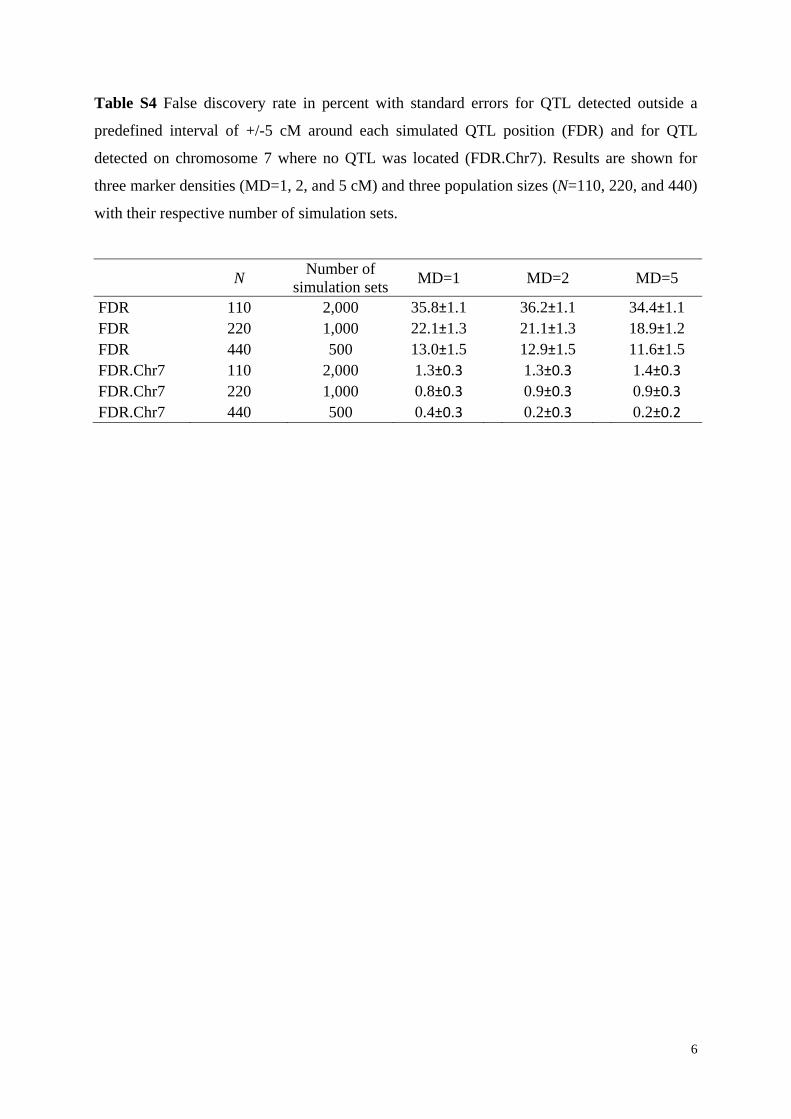
Table S4 False discovery rate in percent with standard errors for QTL detected outside a

predefined interval of +/-5 cM around each simulated QTL position (FDR) and for QTL

detected on chromosome 7 where no QTL was located (FDR.Chr7). Results are shown for

three marker densities (MD=1, 2, and 5 cM) and three population sizes (N=110, 220, and 440)

with their respective number of simulation sets.

N

Number of simulation sets

MD=1

MD=2

MD=5

FDR 110 2,000 35.8±1.1 36.2±1.1 34.4±1.1 FDR 220 1,000 22.1±1.3 21.1±1.3 18.9±1.2 FDR 440 500 13.0±1.5 12.9±1.5 11.6±1.5 FDR.Chr7 110 2,000 1.3±0.3 1.3±0.3 1.4±0.3 FDR.Chr7 220 1,000 0.8±0.3 0.9±0.3 0.9±0.3 FDR.Chr7 440 500 0.4±0.3 0.2±0.3 0.2±0.2

7

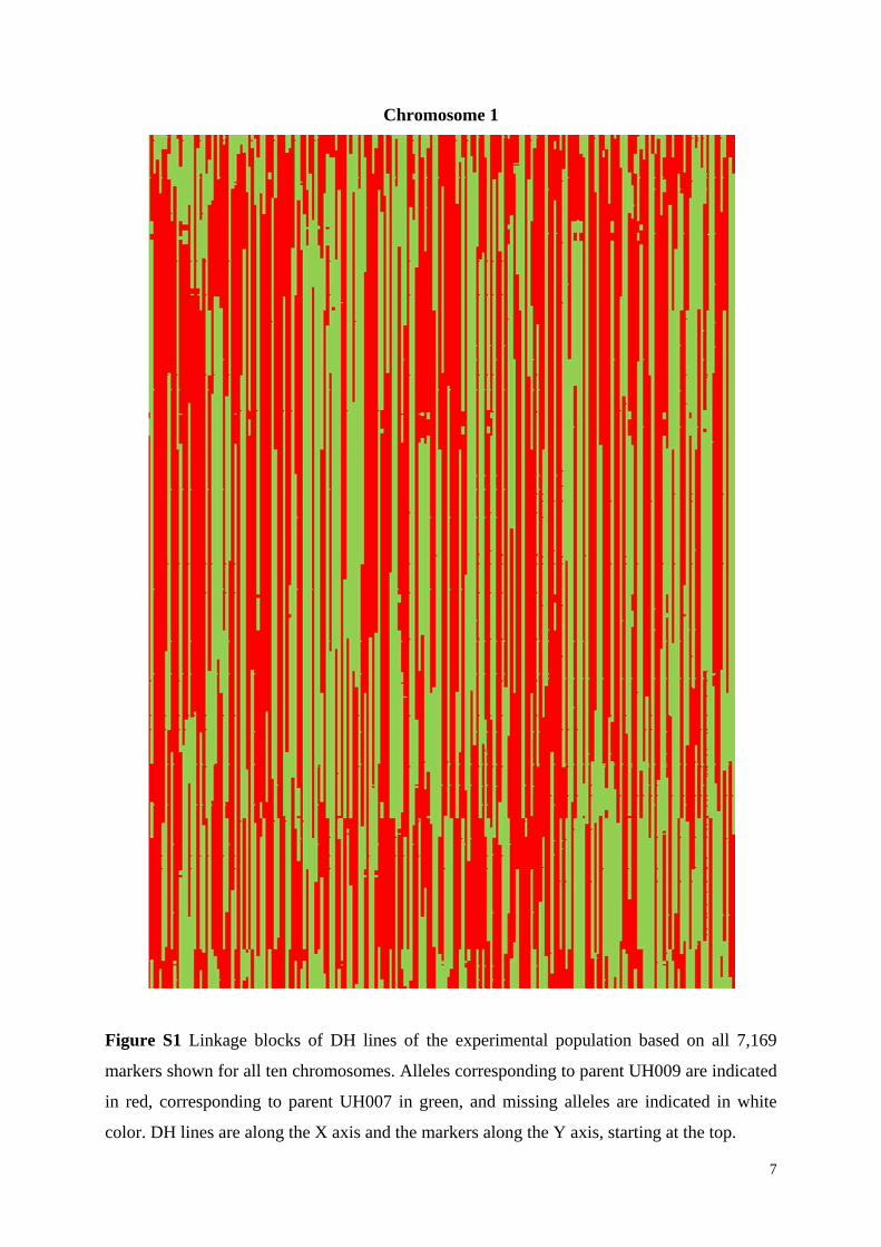
Chromosome 1

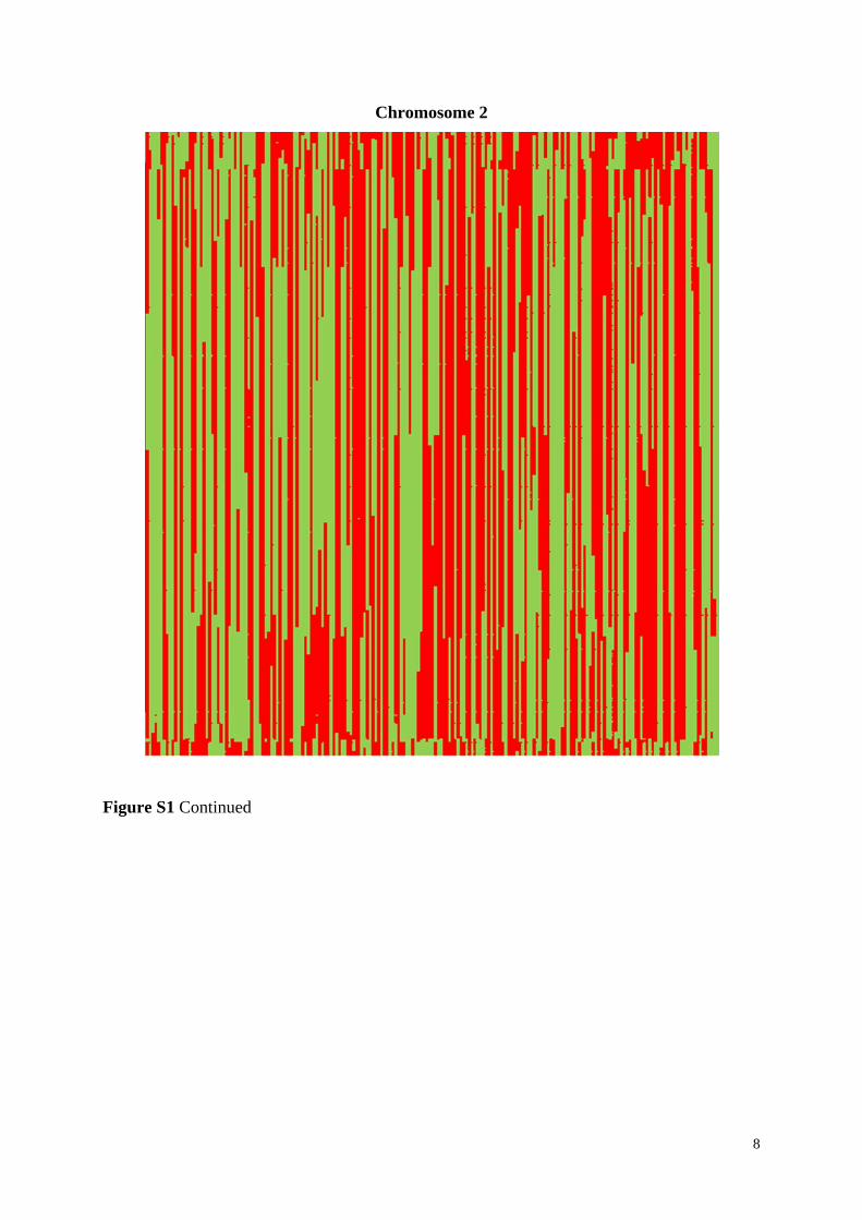
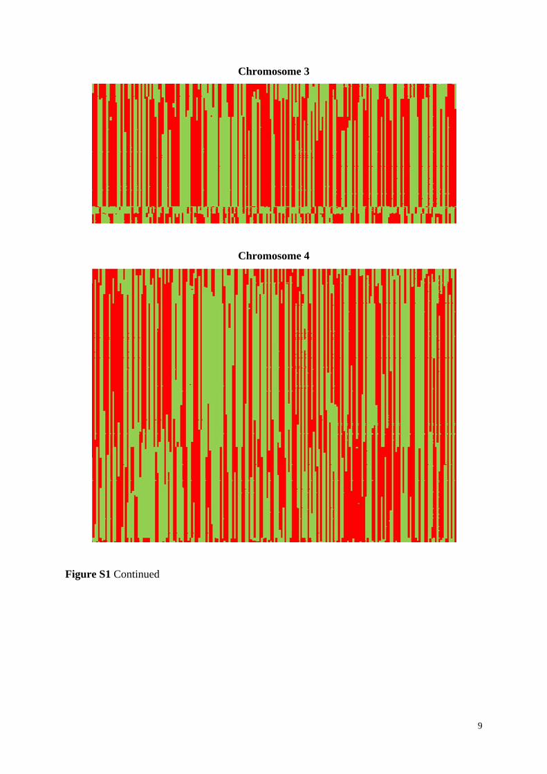
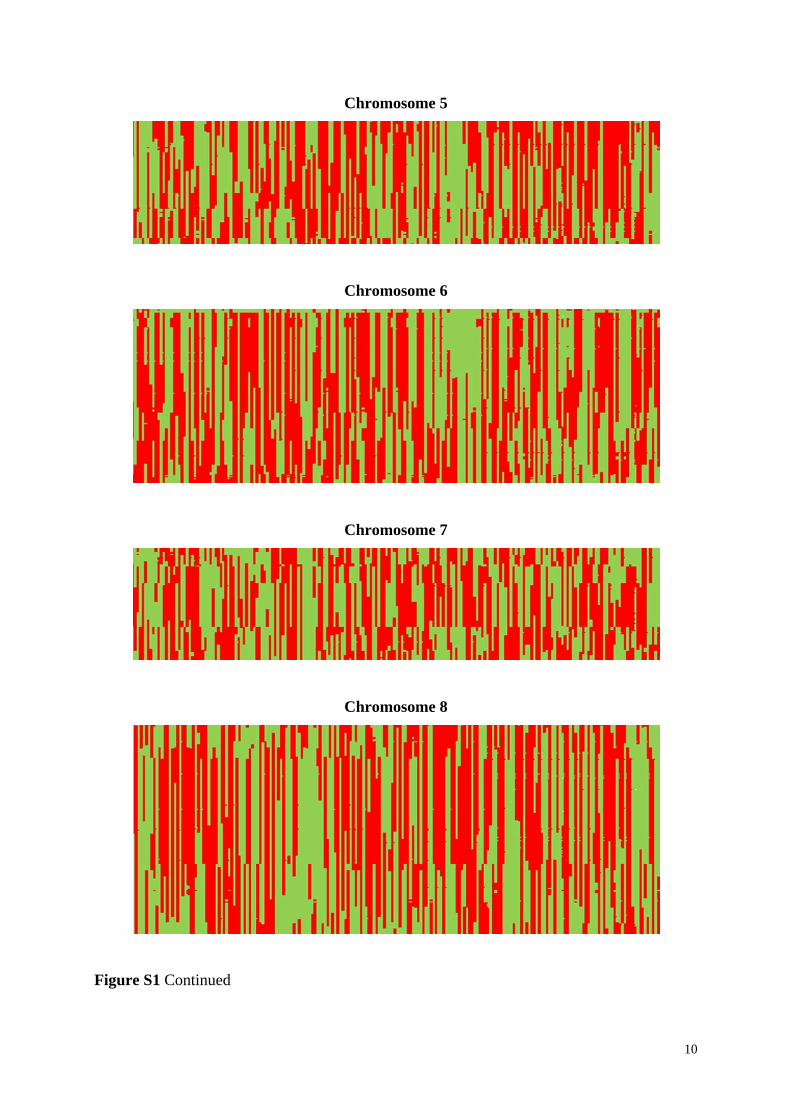
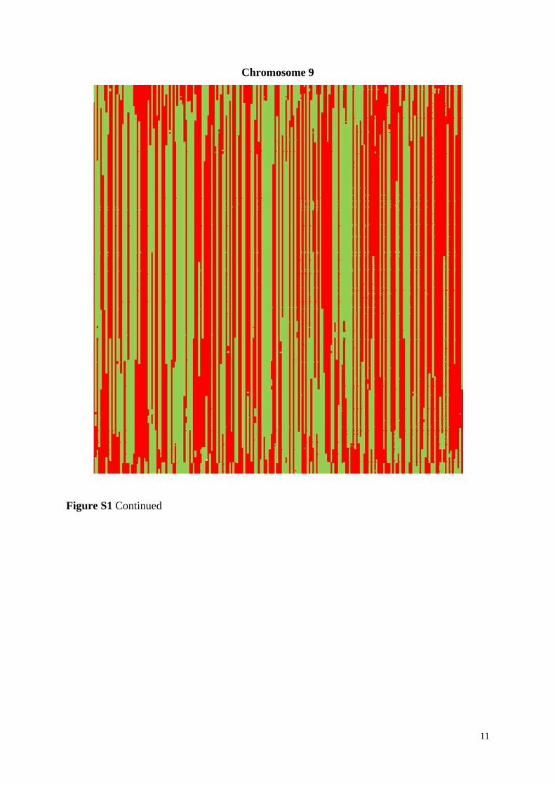
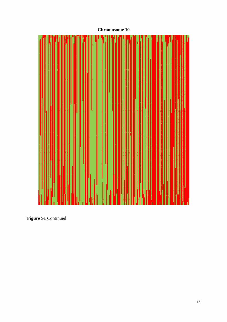
Figure S1 Linkage blocks of DH lines of the experimental population based on all 7,169

markers shown for all ten chromosomes. Alleles corresponding to parent UH009 are indicated

in red, corresponding to parent UH007 in green, and missing alleles are indicated in white

color. DH lines are along the X axis and the markers along the Y axis, starting at the top.

8

Chromosome 2

Figure S1 Continued

9

Chromosome 3

Chromosome 4

Figure S1 Continued

10

Chromosome 5

Chromosome 6

Chromosome 7

Chromosome 8

Figure S1 Continued

11

Chromosome 9

Figure S1 Continued

12

Chromosome 10

Figure S1 Continued

13

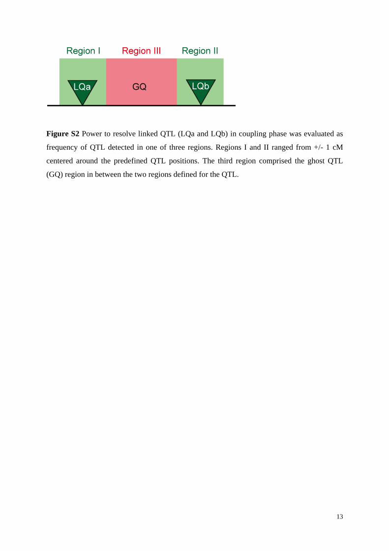
Figure S2 Power to resolve linked QTL (LQa and LQb) in coupling phase was evaluated as

frequency of QTL detected in one of three regions. Regions I and II ranged from +/- 1 cM

centered around the predefined QTL positions. The third region comprised the ghost QTL

(GQ) region in between the two regions defined for the QTL.

14

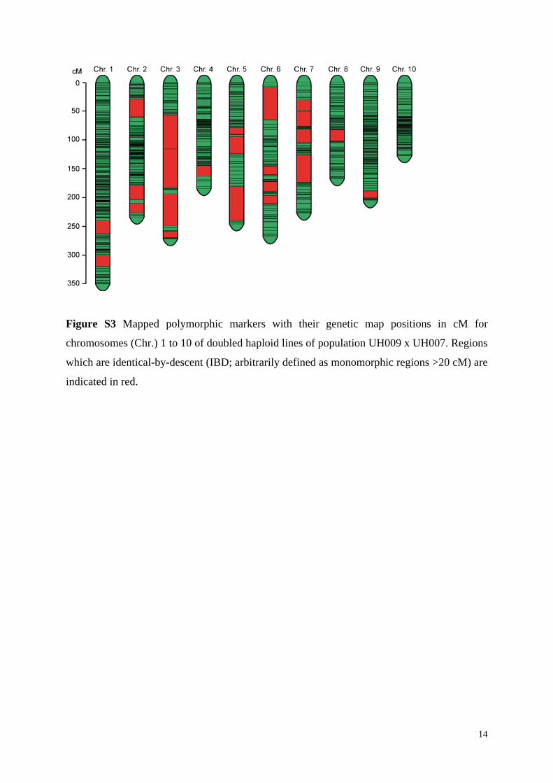
Figure S3 Mapped polymorphic markers with their genetic map positions in cM for

chromosomes (Chr.) 1 to 10 of doubled haploid lines of population UH009 x UH007. Regions

which are identical-by-descent (IBD; arbitrarily defined as monomorphic regions >20 cM) are

indicated in red.

15

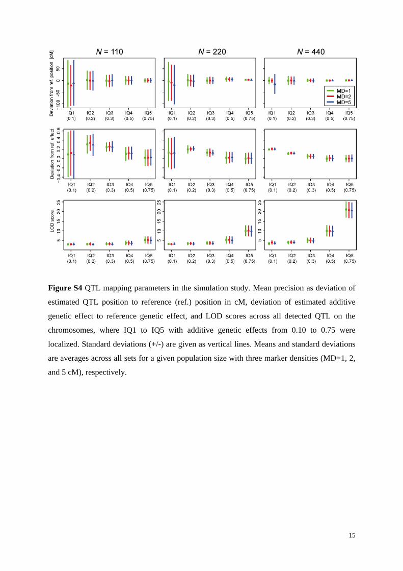
Figure S4 QTL mapping parameters in the simulation study. Mean precision as deviation of

estimated QTL position to reference (ref.) position in cM, deviation of estimated additive

genetic effect to reference genetic effect, and LOD scores across all detected QTL on the

chromosomes, where IQ1 to IQ5 with additive genetic effects from 0.10 to 0.75 were

localized. Standard deviations (+/-) are given as vertical lines. Means and standard deviations

are averages across all sets for a given population size with three marker densities (MD=1, 2,

and 5 cM), respectively.