STANFORD  UNIVERSITY  ENCINA  HALL,  E301  

STANFORD,  CA  94305-­‐6055    

T  650.725.9741  F  650.723.6530

Stanford University Walter H. Shorenstein Asia-Pacific Research Center

Asia Health Policy Program

Working paper ser ies on health and demographic change in the Asia-Pacific

Remittances, Informal Loans, and Assets as Risk-Coping Mechanisms: Evidence from Agricultural Households in Rural Philippines

Marjorie C. Pajaron, Asia Health Policy Program, Stanford University Asia Health Policy Program working paper #32 December , 2012 http://asiahealthpolicy.stanford.edu For information, contact: Karen N. Eggleston (翁笙和) Walter H. Shorenstein Asia-Pacific Research Center Freeman Spogli Institute for International Studies Stanford University 616 Serra St., Encina Hall E311 Stanford, CA 94305-6055 (650) 723-9072; Fax (650) 723-6530 karene@stanford.edu

Remittances, Informal Loans, and Assets as Risk-Coping Mechanisms: Evidence from Agricultural Households in Rural Philippines

Marjorie C. Pajaron

Asia Health Policy Program Stanford University

pajaron@stanford.edu

 

 

1

Abstract

This paper investigates whether agricultural households in the rural Philippines

insure their consumption against income shocks and whether they use migration,

remittances, informal loans, or assets as ex post risk-coping mechanisms. Since these

households have limited access to formal insurance and credit markets, any shocks to

their volatile income can have substantial impacts. Using panel data, and rainfall shocks

as the instrumental variable for income shocks, this paper finds little evidence of effective

risk-sharing within the networks of family and friends. 2SLS, OLS, and SUR estimates

show that only about 16 percent of consumption is insured. While domestic remittances

from other families replace about 51 percent of income decline, informal loans decrease

by about 34 percent. Additional tests, however, reveal that agricultural households

engage in entrepreneurial activity when rainfall increases and children are somehow

protected from the adverse effects of rainfall shocks. Hours spent on own family-operated

businesses likewise increase.

Keywords: Risk-coping, remittances, informal loans, consumption insurance, rainfall shocks, Philippines

JEL classification: O12, Q12, D81, D12, F22, F24

2

1. Introduction

Households in developing countries often face extreme income variation. This is

especially true for households whose income depends on agriculture and other economic

activities susceptible to drastic weather variation. Domestic income shocks may come in

the form of job loss, illness, typhoon, drought, or rainfall variation. It is important to

investigate how households cope with such shocks, especially in poor regions of

developing countries where there is limited access to formal credit, capital, and insurance

markets. Government aid and transfers may also be limited or non-existent.

The main purpose of this paper is to examine how agricultural households in rural

areas of the Philippines insure their consumption against transitory income shocks caused

by rainfall variation. To achieve this, I first examine whether household consumption is

insured against adverse income shocks. Second, if households do insure their

consumption, I investigate whether they use migration, international remittances,

domestic remittances, informal credit, or their assets as ex post risk-coping mechanisms.

I choose to examine the Philippines for four reasons. First, this country is

frequented by typhoons and has experienced natural disasters, such as drought and

flooding, quite often. According to the Philippine Atmospheric Geophysical and

Astronomical Services Administration (PAGASA), during the 59-year period from 1948

to 2006, an average of 10 typhoons occurred in the Philippine Area of Responsibility

annually. There have also been seven drought-causing El Niño episodes since 1968. In

such an environment, rural households whose primary income depends on agricultural

activities face volatility in their income, especially if they depend on rainfall to farm their

3

non-irrigated land. Since rural households have limited access to financial and credit

markets, it is apt to examine what mechanisms they use to cope with risks.1 Part of the

reason why rural households, particularly farmers, face credit constraints is that they are

required to provide land titles as collateral. Those farmers who do not own the land they

farm have a very small chance of accessing loans provided by banks and other financial

institutions. Those who are agrarian reform beneficiaries (ARB) face legal restrictions on

land transfers; along with the limited use of land as collateral and cooperative

membership, they are deemed as risky borrowers.

Second, familial transfers, in the form of international and domestic remittances,

play an important role in the economy of the Philippines. The Philippines was ranked

fourth in total international remittances received in 2009, after India, China, and Mexico

(World Bank, 2012). The inflow of remittances to the Philippines in 2009 amounted to

approximately 15 billion US dollars, which made these transfers the second largest

source of foreign exchange for the Philippines, next to exports of goods and services.

International and domestic remittances also serve as a major source of income for

agricultural households with migrants, affecting their consumption and investment

behavior and their entrepreneurial activities. Data from the Family Income and

Expenditure Survey (FIES) in the Philippines indicated that, on average, international

remittances constituted about 16 percent of the income of agricultural households that

received international remittances in 2006, while domestic transfers, on average,

1 Central Bank of the Philippines (Bangko Sentral ng Pilipinas) reports that only about 7 percent of bank loans were granted to the agriculture, fishing, and forestry industry in 2003. In addition, for the same year, only about 10 percent of the total banks in the Philippines were rural banks, which catered to households and businesses in rural areas.

4

constituted about 50 percent of the income of households that received domestic

transfers.

Third, aside from international migration, rural households employ internal

migration to diversify risk and to insure and smooth consumption when they face adverse

income shocks. Most literature on internal migration in the Philippines use data from the

1980s or 1990s. Quisumbing and McNiven (2005) use 2003-2004 panel data to track

internal migration but focus on one rural area in southern Philippines. I implicitly

analyze the importance of internal migration for all rural households in the Philippines

using the latest national representative survey panel data (2003 and 2006) by

investigating how domestic transfers are affected by income shocks and how they are

used to smooth consumption. I assume that the domestic transfers from other families are

from members who have migrated to urban areas to work. FIES, whose rich panel data

started in 2003, is the major source of household income and expenditure data collected

from all regions in the Philippines.

Fourth, it would be interesting to analyze if agricultural households can

effectively share their risks and which risk-coping strategies help them during bad times.

The reason why I focus on agricultural households is that they are the poorest among the

poor and marginalized groups in the Philippines. The National Statistical Coordination

Board reported that in 2003, farmers and fishermen had the highest incidence of poverty

at 43 percent. In addition, FIES data from 2003 indicate that their average household

income in a year fell below that needed by a five-member household to stay above the

subsistence level.

5

This paper adds to the literature on consumption insurance and risk-sharing by

incorporating migration, international remittances, domestic transfers, informal loans, and

assets into this framework. There have been studies on how international remittances

serve as insurance, independent of other risk-mitigating mechanisms (Lucas and Stark,

1985; Clarke and Wallsten, 2003; Yang and Choi, 2007). To the best of my knowledge,

this is the first paper that investigates the use of international remittances as consumption

insurance in the context of other mechanisms: domestic transfers, informal credit, and

sales of assets among them. In doing so, this paper determines the relative importance of

each risk-coping mechanism and whether they affect or crowd one another out.

To test this empirically, I analyze whether household income affects household

consumption. I use the panel data of national representative survey (FIES) from the

Philippines for the years 2003 and 2006. I apply first differencing to eliminate fixed

effects problems. Since household income is endogenous, which may be due to reverse

causation, ordinary least squares (OLS) estimates may result in a biased estimate. Using

an instrumental variable for household income may resolve this issue, provided that the

instrument used is strong and that it satisfies two conditions: it is exogenous and it is

partially correlated to household income. I use rainfall shocks as instruments since

agricultural households in the Philippines depend on rainfall significantly, especially

those farming non-irrigated land. Rainfall shocks are measured as the difference in

rainfall experienced by agricultural households in 2003 and 2006. Using great circle

distance (GCD), the closest weather station to the household is determined and the

rainfall amount recorded in that weather station is assigned to the household. The

instruments, after experimenting with the econometric specification and different

6

measures of rainfall, fall below the conventional weak instrumental variable threshold

suggested by Staiger and Stock (1997), and Stock and Yogo (2002). Focusing on the

reduced form instead, the OLS estimates indicate that the null hypothesis of full

consumption insurance can be rejected, however, partial insurance still exists. I use

partial insurance to refer to situations where any form of consumption smoothing exists.

The results indicate that rainfall shocks adversely affect income and consumption, which

is contrary to the findings of Yang and Choi (2007), who use a Philippine data set from

1996 and 1997. One possible reason for this is that in 1997-1998 the Philippines

experienced El Niño such that any rainfall was beneficial not just to farmers but also to

entrepreneurs who rely on agricultural products for raw materials, hence the positive

impact of rainfall shocks on household income.2 Another explanation is that in 2006, the

Philippines experienced a high volume of rainfall due to record-breaking typhoons that

hit the country such that more rainfall caused a decline in the income of agricultural

households.

Based on the results of this paper, it can be inferred that OLS estimates, which are

consistent with the IV estimates, show that agricultural households insure about 16

percent of their consumption. This result may also mean that 16 percent of consumption

is smoothed or that 16 percent of income shocks are insured. Given this finding, I explore

five possible risk-coping mechanisms that households employ to smooth their

consumption. Domestic transfers are positively affected by rainfall shocks while informal

loans are adversely affected; migration, international remittances, and assets are not

impacted by rainfall shocks. Domestic transfers replace about 51 percent of income

2 The El Niño phenomenon is an example of climate variability; it is characterized by a dry season lasting for 12 months or more, and the late start and early termination of the rainy season.

7

decline; informal loans, about 34 percent. The net change in available resources is about

16 percent of income decline. SUR estimates indicate similar results, which implies that

the error terms among the different regressions for risk-coping strategies are uncorrelated.

These results are robust when rural households, regardless of the type of

employment of household head, are used. The implication of these results is that families

who provide domestic remittances to agricultural households are most likely located in

areas unaffected by similar rainfall shocks, hence their ability to provide financial support

(Paulson, 2000). Conversely, families who provide informal loans may be experiencing

the same shocks and are unable to effectively share risks with other families. The results

on informal loans are contrary to the results found by Fafchamps and Lund (2003), who

conducted a risk-sharing analysis of villages in the northern Philippines and found that a

quasi-credit model of informal risk-sharing fit their data. One possible reason for this

difference is the types of shocks that Fafchamps and Lund (2003) used, which are

idiosyncratic shocks specific to households, such as unemployment of head or spouse,

acute sickness, and funeral. They did not find risk-sharing within the village, but found

that networks of family and friends did share risks using a combination of gifts and no-

interest loans. In addition, they also found that some shocks are uninsured while some are

better insured. Another result of this paper, which is inconsistent with the existing papers

on income shocks and international remittances (Clarke and Wallsten, 2003; and Yang

and Choi, 2007), is the insignificance of international remittances in insuring household

income. This result can be attributed to the fact that in the dataset there are only a few

agricultural households that have migrant members abroad (about 13 percent). This is

not surprising since sending a migrant abroad requires a large fixed cost, which most

8

agricultural households cannot afford owing to their credit and financial constraints. In

addition, there is little variation in the relationship between remittances and rainfall

shocks (Figure 1).

I analyze other possible sources of income for agricultural households since a 16-

percent replacement rate may be insufficient for them to effectively cope with risks. I

find that they also rely on wholesale and retail sales (including sidewalk vending, market

vending, and peddling) when they encounter an increase in rainfall shocks. I also

examine if their labor supply (hours worked) is affected by shocks and find that

agricultural households tend to focus more of their time on own-family operated farm or

business without pay to deal with shocks. Finally, I want to know whether children are

somehow protected against shocks – their labor supply and schooling are unaffected

while their education expenditures actually increase by about 1 percent.

This paper is organized as follows. Section 2 tests whether agricultural

households in the Philippines follow the full consumption insurance theory, using two

stage least squares (2SLS) and OLS. Section 3 analyzes whether they use familial

transfers (international and domestic transfers from migrant members), informal loans,

and assets as risk-coping strategies to insure their consumption against income shocks,

using OLS. This section also includes the analysis of the impact of rainfall on net

available resources for agricultural households by estimating the sum of all risk-

mitigating strategies. Section 4 focuses on robustness checks, including using SUR

specification and omitting the interaction of time-invariant household characteristics and

a time dummy. Section 5 examines the response of different types of households (rural or

urban; migrant or non-migrant) to rainfall shocks. Section 6 explores additional

9

questions, including whether entrepreneurial activities, household labor supply,

children’s labor supply and schooling, education, health, and durable goods expenditures

are affected by rainfall shocks. Section 7 concludes.

2. Full insurance of consumption  

Full consumption insurance is possible if households efficiently allocate their

risks within their networks of family and friends. There is evidence that Philippine

households receive help in response to income shocks mostly from such informal

networks (Fafchamps and Lund, 2003; Yang and Choi, 2007), making this an important

kind of risk-sharing to investigate.

A Pareto-efficient allocation of risk exists if household consumption only depends

on the average consumption of networks of family and friends, and not on the

household’s own income. This implies that only aggregate risk faced by these networks

affects household consumption. Idiosyncratic income shocks are irrelevant because they

are completely insured within the networks. Empirical studies often reject efficient

allocation of risk for certain types of shocks and households because of this strong

implication (Cochrane, 1991; Mace 1991; Townsend, 1994). Partial Pareto-efficient

allocation of risk, however, may exist and households may employ risk-coping

mechanisms.

10

2.1 Theory for full insurance of consumption

To test the existence of full consumption insurance among networks of family and

friends, let i=1,…,N be the index of households, each with an uncertain income isty >0,

where s∈S is the state of nature, and t∈T is the index for time. Assume that each

household has an instantaneous utility function ( )ii stU c that is separable over time and

twice continuously differentiable, where cist is the consumption of household i at state of

nature s and at time t. To achieve a Pareto-efficient allocation of risk, the weighted sum

of the utilities of household i is maximized, given that the weight of household i in the

Pareto program is λi, where 0< λi<1, ∑λi=1. Suppose that each household has a constant

absolute risk aversion utility function: ( )ii stU c = -(1/γ) exp (-γ cist). Pareto-efficient

allocation of risk exists if the ratio of the marginal utilities in any state of nature is equal

to a constant; in this case, it is equal to the ratio of Pareto weights (λi). Following

Cochrane (1991), Mace (1991), and Townsend (1994), a relationship between individual

household i’s consumption and average consumption across households can be expressed

as:

1

1 ln( ) (1/ ) ln( )N

ist st i j

jc c Nλ λ

γ =

⎡ ⎤= + −⎢ ⎥

⎢ ⎥⎣ ⎦∑ (1)

Equation (1) shows that household i’s consumption depends only on the

networks’ average consumption stc and Pareto weights. Household income does not

affect household consumption when households efficiently pool risks. Therefore, if

11

consumption is regressed on income, the estimated coefficient of income should be

insignificant if full consumption insurance holds. To empirically verify this, I follow

Fafchamps and Lund (2003) and decompose household income (yist) into a transitory

component of income (yiTst) and permanent component of income (yiP):

yist=yiT

st+yiP (2)

Along with Pareto weights, the permanent component of income is not dependent

on state of nature and can be regarded as a function of household fixed effect (ω i). Since

average level of consumption in the networks does not vary across households, a dummy

variable for time (d t ) is used as a proxy (Ravallion and Chaudhuri, 1997; Fafchamps and

Lund, 2003; Yang and Choi, 2007). Given these assumptions and allowing for a random

component, uit, error term with zero mean, consumption insurance can be empirically

tested using the following equation:

cist= d t +yiT

st +ω i + uit (3)

where transitory income, yiTst, is instrumented using rainfall shocks. There are three

possible scenarios. First, if the estimated coefficient of yiTst is equal to one, then the null

hypothesis of full consumption insurance can be rejected. Second, if this estimate is

between zero and one, then there exists some degree of consumption insurance. Third, if

the estimate is zero then full consumption insurance cannot be rejected.

12

2.2 Description of data for full insurance of consumption

2.2.1 Household survey data

I use household data for 2003 and 2006 from Family Income and Expenditure

Survey (FIES) to construct a panel data. FIES is a nationwide survey conducted every

three years by the National Statistics Office (NSO) as a rider to the Labor Force Survey

(LFS). FIES is the main source of data on Philippine household income and expenditure

levels. In 2003, the sampling design of FIES used a new master sample – the 2003

Master Sample for Household Surveys – which was based on the 2000 Census of

Population and Housing. This master sample provided a scheme where the same sample

households could be used in succeeding survey years. As of this writing, FIES survey

data for 2003 and 2006 are the only official data from which a panel data can be

constructed and 2009 is yet to be released.

Table 1 depicts the characteristics of the panel data on agricultural households in

rural areas. The agricultural households are defined using the 2003 FIES survey data to

address possible selection bias and prevent household classification from being

endogenous to rainfall if the households were based on 2006 data. There are 721

agricultural households, which constitute about 58 percent of rural households. Of these

agricultural households, 611 (85 percent) planted crops as their main source of income

and 110 households (15 percent) engaged in other agricultural activities such as farming

of animals, animal husbandry, fishing, and logging. Most household heads only

completed primary education (about 65 percent) in 2003 and the average household size

was five. Table 2 depicts the definition, mean, and standard deviation of the rainfall and

13

outcome variables. On average, the annual total household income of agricultural

households increased by about 33 percent between 2003 and 2006, whereas total

household expenditures increased by approximately 28 percent. Rainfall variables are

discussed in the next section.

2.2.2 Rainfall data

Rainfall data from PAGASA are used as a measure of shocks to the transitory

income of Philippine households. Several authors, such as Paxson (1992), Paulson

(2000), and Yang and Choi (2007), have used rainfall shocks as shocks to income.

Monthly and annual rainfall data come from the 45 weather stations of PAGASA, which

are located in various cities and municipalities. Rainfall shocks are derived by subtracting

the annual rainfall (in millimeters) recorded at each of the 45 weather stations in 2003

from the same station’s annual rainfall in 2006.

I assign rainfall shocks to households based on their distance from the nearest

weather station using great circle distance. Great circle distance between two points, in

mathematics, is the shortest distance over the surface of a sphere. In addition, the climate

type of the household’s city or municipality is matched with the climate type of the

nearest weather station’s city or municipality. According to PAGASA, if the municipality

(or city) of the household, and the municipality (or city) of the nearest weather station

have a similar climate type, and the distance between them is less than about 50

kilometers, then the rainfall shocks from the weather station can be assigned to the

household. If there are two or more weather stations that meet the criteria, I average

14

rainfall shocks and assign the average to the household. If there are no weather stations

close to the household (within the 50-kilometer range), then this household is deleted

from the analysis. This last condition will be relaxed later and households will not be

dropped from the analysis to increase the sample size and to improve the instrumental

variable used.

On average, agricultural households experienced more rainfall in 2006 than in

2003, by about 0.12 meters (Table 2). This can be attributed to typhoons that crossed the

Philippines in 2006. According to PAGASA (2011), that year’s typhoon Milenyo is one

of five that caused the most damage to properties in the Philippines since 1948. One of

the five strongest typhoons in the same period, typhoon Reming, hit the Philippines in

2006 as well. Consequently, the average rainfall in 2006 deviated more from the

historical mean than the average rainfall in 2003. The 2006 rainfall was greater by 0.15

meters than the historical mean rainfall from 1974 to 2000, whereas rainfall in 2003

deviated by only about 0.05 meters.

2.3 Estimation strategy for full insurance of consumption

Estimating Equation (3) to test full consumption insurance using OLS may result

in a biased estimate for the transitory component of income, which can be attributed to

reverse causation and fixed effects. Reverse causation implies that household income

may be a function of household consumption itself. For example, higher food

consumption may translate into more nourished household members, more productive

work, and higher income. A study of farm households in the Philippines shows that food

15

consumption serves as a nutritional investment that affects marginal productivity of

members (Dubois and Ligon, 2005). Fixed effects mean that there exist unobserved

variables, such as preferences to work or not to work, that may influence both household

income and consumption.

Since there are two observations for each household, the first difference, for

which 2003 data are subtracted from 2006 data, can be derived to eliminate time-

invariant household fixed effects. Reverse causation is addressed using change in rainfall

shocks as the instrumental variable for change in income. Rainfall shocks are a good

measure of income shocks since agricultural households rely heavily on rainfall,

particularly households that farm non-irrigated land. According to the National Irrigation

Administration (2011), in 2006 only 46 percent of the total irrigable land in the

Philippines was irrigated, which means that agricultural activities on the remaining land

depended on rainfall.

Two conditions must be satisfied to make the change in rainfall a strong

instrument: it should be partially correlated to household income and uncorrelated to the

disturbance term in Equation (3). Otherwise, weak instruments may lead to a substantial

bias in the instrumental variable estimators and hypothesis tests that have large size

distortions (Stock and Yogo, 2002).

To test the first requirement, change in income is regressed on change in rainfall.

The second condition for a strong instrumental variable is satisfied because the rainfall

shocks variable is exogenous to the causal system that constitutes how household income

affects household consumption. This means that the factors that affect rainfall variation

16

are determined outside of Equation (3). The preceding section shows whether the

instrumental variable I am using is strong.

2.4 Results for full insurance of consumption

2.4.1 Instrumental variable estimation for full insurance of consumption

I measure household income (net of remittances) as a change from 2003 to 2006

divided by initial household income in 2003. Similarly, household expenditure is

measured as change divided by initial household expenditure in 2003. I choose to

express consumption and income this way, instead of taking the logs, to be consistent

with how I measure risk-coping mechanisms that have zero values. In addition, I can

interpret estimated coefficients as a percentage of the initial household income.

I use a time dummy (dt, which is equal to one if t = 2006, zero otherwise) in my

regression analysis to account for time effects that affect all households, such as price

inflation. I also include time-variant household characteristics (Xti), such as household

size and age of the household head, and household characteristics (Vi), measured in 2003,

that did not change much over time, such as marital status and the completed education of

household head. Marital status remained the same for approximately 94 percent of the

agricultural households in rural areas, so I consider it a time-invariant household

characteristic. I interact time-invariant household characteristics with a dummy variable

for time (dt* Vi) to allow time effects to vary according to household characteristics, such

as nationwide economic shocks that may have different effects on educated and less-

educated households (Yang and Choi, 2007). I initially estimate the following Equation

17

(4), which is derived from Equation (3), by 2SLS to investigate if household income,

instrumented by rainfall shocks, affects household expenditures.

Δci2 0 0 6 = δ 0 +β 1Δy iT

2 0 0 6+β 2Δ Xi 2 0 0 6 + β 3 d2006*Vi+Δui

2006 (4)

where δ 0 = δ 0Δd2006 given that dt is equal to one if t = 2006, and zero otherwise.

I cluster standard errors by province to address serial correlation among error

terms of households belonging to the same province. Table 3 shows the results of 2SLS

estimation for agricultural households. First stage regression, reported in the first

column, indicates that the estimate for rainfall shocks is significantly different from zero.

An increase of 500 millimeters of rainfall results in approximately a 6 percentage point

fall in household income (first column). The second column shows the results of second

stage regression where the estimated coefficient of income is positive and less than one,

and statistically significant at the 1% level. This means that some degree of consumption

insurance exists. The decrease in household consumption is not as much as the decrease

in household income: a 10 percentage point decline in household income leads to

approximately a 8.4 percentage point decrease in household consumption. This suggests

that about 16 percent of household consumption is insured.

However, the results should be interpreted with caution. In the first stage

regression, which tests for the relationship between rainfall shocks and household

income, the F-statistics can tell us whether the first condition for a strong instrumental

variable is satisfied. The F-statistics, which is about 3.7, suggests that the instrumental

variable is weak since it is below the weak instrumental variable threshold of 10 (Staiger

and Stock, 1997; Stock and Yogo, 2002). This means that rainfall shocks and income are

18

weakly correlated, which may lead to a large asymptotic bias in the instrumental variable

estimator even if the second condition is satisfied.

I use several strategies to address the issue of weak instrumental variable. First, I

change the assignment of rainfall shocks to households by including households whose

distance from the closest weather station exceeds 50 kilometers. This increases the

sample size and although this may introduce some noise, there may still be signal that can

be derived from here. I then add instrumental variables for rainfall at the next two closest

weather stations to improve the F-statistics (Maccini and Yang, 2009). Table 4 shows

that the F-statistics for agricultural households actually decreases to about 1.0. All

succeeding IV experiments and their corresponding F-statistics are displayed in Table 4.

Second, I experiment with quarterly rainfall variables and seasonal rainfall

variables as instrumental variables (Paxson (1992); and Yang and Choi (2007)). This

exercise may capture more variation in rainfall and may improve the instrumental

variables. The results show that both sets of rainfall shocks are weak instruments for

household income, with F-statistics at 1.4 for quarterly rainfall variables and 2.2 for

seasonal rainfall.

Third, I add the interaction of rainfall shocks and different categories of other

agricultural activities other than planting crops, such as farming of animals, animal

husbandry, fishing, and logging as instrumental variables. These other agricultural

groups may be differentially affected by rainfall and, therefore, when interacted with

rainfall shocks may provide variation in rainfall shocks within a municipality. In

addition, the inclusion of these interaction terms may yield a stronger first stage, since

rainfall matters more in areas with households more engaged in rain-fed agriculture than

19

in other areas. However, the sample size is small given that only about 15 percent of the

agricultural households are engaged in other agricultural activities. These exercises did

not yield a stronger first stage, and the F-statistics of 2.6 remains below the conventional

cut-off. Even after interacting quarterly and seasonal rainfall variables separately with

different types of other agricultural activities, the F-statistics are at about 1.6 and 3.0,

respectively.

Fourth, I experiment with the functional form and consider a quadratic

relationship between income and rainfall shocks. Change in rainfall and change in rainfall

squared are individually significant, however the F-statistics is small, at 4.5.

Fifth, I include typhoon variables as explanatory variables to control for the

possibility that it drives the negative effect of rainfall on income and to verify whether it

improves the F-statistics. For IV estimation, I measure typhoon as the change in the

number of typhoons that hit the area over the past year. The estimated coefficient on

rainfall becomes statistically insignificant although it remains negative (Table 6, Column

3), while the F-statistics is at 2.8, which is still below the cut-off. In a later section, I

discuss further if typhoon alters the relationship of rainfall and household income.

2.4.2 Reduced form estimation for full insurance of consumption

Given that rainfall shocks prove to be a weak instrument for household income, I

focus instead on the reduced form and I use rainfall shocks as an explanatory variable for

both household income and consumption. I estimate the following equations using OLS:

20

Δyi2 0 0 6 =ξ 1 +ξ 2ΔRF i

2 0 0 6+ξ 3ΔXi2 0 0 6+ξ 4 d2006*Vi +Δvi

2006 (5)

Δci2 0 0 6 =δ 1 +δ 2ΔRF i

2 0 0 6+δ 3ΔXi2 0 0 6+δ 4 d2006*Vi+Δui

2006 (6)

where RFi2006 is rainfall shocks, which, along with the rest of the independent variables,

are similar to those used to estimate Equation (4) originally.

In Equation (5), a negative and significant estimate of ξ 2 suggests that an increase

in rainfall shocks has an adverse effect on household income. In Equation (6), if δ 2 is

equal to zero then the null hypothesis of full consumption insurance cannot be rejected.

If instead, δ 2 is negative and significant, then full consumption insurance is rejected.

However, some degree of insurance may exist if both δ 2 and ξ 2 are negative,

significant, and ξ 2 >δ 2 , in absolute terms. This suggests that household consumption

does not fall as much as income does when rainfall shocks increase, because households

may be using risk-coping strategies to mitigate the adverse effects of income shocks.

OLS regression results show that partial consumption insurance exists (Table 5).

An increase of 500 millimeters of rainfall results in a 5.8 percentage point decline in

household income and a 4.9 percentage point fall in household consumption. These

results show that, given a similar increment in rainfall, the decline in household

consumption is less than − or about 84 percent of − the decline in income. This suggests

that about 16 percent of consumption is insured, which is consistent with the 2SLS

results. The high co-movement between income and consumption may be attributed to

the damage caused by a typhoon such that there is limited available crops to consume.

This may be true if imperfect inter-municipality markets exist; a municipality devastated

21

by a typhoon cannot rely on another locality for provision. In effect, municipalities may

not be able to insure each other especially if the typhoon impacts most areas.

Contrary to my findings, Yang and Choi (2007) found a positive effect of rainfall

shocks on household income in their 1996-1997 study of households in the Philippines.

There are three possible reasons for this inconsistency: first, as mentioned above, in 2006

the Philippines was hit by two super typhoons – one was recorded as the strongest since

1948; the other caused the most damage to properties. The rainfall associated with these

typhoons caused harm to crops and other livelihoods of agricultural households. To test

this, I add two typhoon variables in both Equations (5) and (6) – one is a change in an

indicator variable that measures whether typhoons have occurred in the municipality in

the past year, the other measures the change in the number of typhoons that hit the area in

the past year. Table 6 shows the coefficient estimates for rainfall shocks when typhoon is

measured as a change in an indicator variable (Columns 1 and 2), as a change in the

number of typhoons (Columns 3 and 4), and when both typhoon variables are included in

the regression (Columns 5 and 6). In all regressions with income as the outcome

variable (Columns 1, 3, and 5), income remains adversely affected by rainfall.

Furthermore, the results in Columns 1 and 2 are consistent with the results in Table 5

when the reduced form is estimated without typhoons. The rainfall shocks coefficients

are negative and statistically significant at 10 percent for both income and consumption

regressions. Keeping everything else constant, the results indicate that even after

controlling for typhoon, both household income and consumption decrease when rainfall

shocks increase.

22

Since the inverse relationship of rainfall shocks and household income cannot be

attributed to typhoon, another explanation for the positive relationship found in the 1996-

1997 study is that the Philippines experienced El Niño from 1997 to 1998. Based on a

report presented by the Asia Pacific Disaster Management Center, the Philippines

experienced a dry spell between June and October 1997 that lingered until mid-

September 1998. I can conjecture that during this period any rainfall was good rainfall

and beneficial not just to farmers but also to entrepreneurs who relied on agricultural

products for raw materials. During the 1997-1998 El Niño, 68 percent of the country was

affected by the drought compared to only 28 percent in 1972 and 16 percent in 1982.3 Six

drought events happened during the 1960-1995 period, but the economic impact was not

as prominent compared to 1997-1998. For example, the volume and value of rice

production increased from 1994 to 2008, with a dip in 1998 as a result of El Niño

(Bureau of Agricultural Statistics, 2011).

Third, and related to the second point is that the volume of rainfall experienced by

the Philippines in 2006 was much higher relative to that in 1997. The change in rainfall

between 2003 and 2006 is 0.12 meters, implying a wetter year in 2006 while the change

in rainfall was negative for both dry and wet seasons between 1996 and 1997, suggesting

a dryer year in 1997. This supports the explanation above that the positive relationship

found between rainfall shocks and income may be attributed to drought in 1997; an

increase in rainfall was deemed beneficial for farmers and entrepreneurs relying on

agricultural products.

3 According to PAGASA, there were seven episodes of El Nino since 1968 (1968-1969, 1972-1973, 1976-1977, 1982-1983, 1986-1987, 1990-1995, and 1997-1998).

23

3. Risk-coping strategies

Given that agricultural households insure their consumption to some degree, I

investigate the first three ex post mechanisms that they may use to insulate consumption

against shocks to income: transfers from family and friends, informal loans from other

families, and profits from selling their own assets. Data from FIES 2003 show that 77

percent of the agricultural households in the Philippines use one or a combination of

these risk-coping strategies, which several different empirical studies also find to be in

use. Some authors investigate risk-sharing among villagers through credit (Platteau and

Abraham, 1987; Udry, 1990). Others examine how self-insurance through saving, along

with the purchase and sale of assets, helps smooth consumption (Deaton, 1992;

Rosenzweig and Wolpin, 1993). The risk-coping mechanisms that I examine are closest

to those used by Fafchamps and Lund (2003). However, I distinguish domestic from

international transfers to account for the role of international migrants in insuring origin

households and use the national representative survey panel data.

3.1 Theory for risk-coping strategies

Assume that household consumption is financed by own income ( isty ),

remittances from a household member living abroad ( istr ), domestic transfers from

family members and relatives (t is t), loans from other families and friends ( istl ), and sale

of assets (aist):

24

cis t = yi

s t+ r is t+ t i

s t+ l is t + ai

s t (7)

Then Equation (1) can be expressed as:

1

1 ln( ) (1/ ) ln( )N

i i i i ist st st st st st i j

jr t l a y c Nλ λ

γ =

⎡ ⎤+ + + = − + + −⎢ ⎥

⎢ ⎥⎣ ⎦∑ (8)

To empirically test Equation (8), household income (yist) is decomposed into

uninsurable permanent income ( iPy ), which is independent of state of nature, and

insurable transitory income ( iTsty ) given a state of nature s at time t. Year dummy (d t )

serves as a proxy for average consumption while household fixed effect (ωi) is used as a

proxy for permanent income and welfare weights. With these in mind and allowing for

zero-mean error term, εit, Equation (8) then translates into:

r is t+ t i

s t+ l is t + ai

s t=d t +y iTst +ωi + εi

t (9)

To empirically test Equation (9), I use transitory income shocks, measured as

rainfall shocks, to determine whether they affect the outcome variable. If the coefficient

estimate is positive and significant, then households use the dependent variable as a tool

to insure consumption against income shocks.

25

3.2 Description of data for risk-coping strategies

To test which risk-coping mechanisms households depend on, I examine the same

panel data (for 2003 and 2006) I used in full consumption insurance analysis. Likewise,

the same rainfall data are assigned to households.

Table 2 displays the mean, standard deviation, and definition of the outcome

variables. On average, international remittances and net assets decreased in 2006.

International remittances declined by approximately 950 pesos, while net assets,

measured as the sale less purchase of real and financial assets, fell by 336 pesos. Real

assets encompass land, real estate, and other personal assets such as jewelry, whereas

financial assets constitute profits from the sale of stocks and real assets. Domestic

transfers, loans from other families, and net loans all increased. Domestic transfers

increased by about 1,270 pesos, while loans from other families rose by approximately

566 pesos. Net loans, defined as loans received from other families less loans given to

other families, increased by 938 pesos.

3.3 Reduced form estimation for risk-coping strategies

Given that rainfall shocks are weak instruments for household income, I focus on

the reduced form here as well. To determine whether remittances, loans, and assets are

used as ex post mechanisms to insulate consumption, they are regressed separately on

rainfall shocks. The risk-coping tools are measured as a change from 2003 to 2006

divided by income in 2003 so that they can be interpreted as the replacement rate or the

26

percentage of a fall in income that is replaced (Yang and Choi, 2007). I estimate the

following Equation (10) using OLS :

Δoi2006 = π1 + π2 ΔRFi

2006 + π3 ΔXi2006 + π4 d2006*Vi + Δεi

2006 (10)

where Δoi2006 is the change in the outcome variable (international remittances,

domestic transfers, loans, net loans, and net assets); π1 =π1 Δd t given that d t is equal to one

if t=2006 and zero otherwise; Xi2006 is time-variant household characteristics (age of

household head and household size); Vi is a vector of household characteristics, defined

in 2003, that did not change over time (household head’s marital status and completed

education); and interaction of a time dummy and time-invariant household

characteristics (d2006*Vi).

If the estimated coefficients of rainfall shocks are significantly different from zero

and positive (π 2 > 0) then households use the dependent variable as a risk-coping

mechanism. The OLS results of testing which risk-mitigating mechanisms households

depend on are displayed in Table 7. The standard errors are clustered by province. The

estimated coefficient on rainfall shocks is positive and statistically significant at the 5%

level for the domestic remittances regression, which suggests that these transfers serve as

insurance when rainfall increases. Although this estimate is small in magnitude (0.059),

when compared to the rainfall shocks estimate in income regression (-0.116) in Table 5,

this can be interpreted as replacing the income decline by roughly 51 percent given an

increase of 500 millimeters in rainfall. While the rainfall shocks estimates are

statistically insignificant in the international remittances and assets regressions, they are

27

negative and statistically significant in the loans and net loans regressions. There are five

possible reasons for this inverse relationship between informal loans and rainfall shocks.

First, it is possible that loans are instead used as an ex ante mechanism to insulate

consumption. During a good state of nature, households may borrow more money to

invest in technologies and crops that are not susceptible to weather variation. This is to

ensure a steady stream of income even during a bad state of nature. To test this, I need

another period to see if informal loans from other families increase when they encounter

good shocks to their income. This is reserved for further studies since the 2009 results of

FIES are unavailable as of this writing.

Second, lenders may be risk averse and relatively less willing to lend during a bad

state of nature due to the creditworthiness of the borrowers. To empirically test this, I

divide the sample, using 2003 wealth data, into wealthy and unwealthy households, then

regress loans and net loans on rainfall shocks. Wealthy households are defined as those

whose income are above the average while unwealthy households are those with income

below or equal to the mean. If the coefficient estimates on rainfall shocks are negative

and significant for unwealthy households but insignificant for wealthy households, then

procyclical lending standards may explain why loans and net loans increase during bad

state of the nature. Table 8 shows the results of this test for unwealthy and wealthy

households separately. While the estimates on rainfall shocks are negative and

statistically significant at the 5 percent level for the unwealthy households in loans and

net loans regressions (Columns 1 and 2), they are negative and insignificant for wealthy

households (Columns 3 and 4). It can be inferred that it is the unwealthy agricultural

28

households who are affected by these lending standards and are unable to borrow money

from other families when they encounter rainfall shocks.

Third, borrowers and lenders may be experiencing similar rainfall shocks,

particularly if they belong to the same municipality. If so, their incomes most likely have

a high covariance, which reduces the effectiveness of local risk-sharing arrangements

(Bardhan and Udry, 1999). I cannot explicitly verify this conjecture since the national

survey that I use (FIES) does not contain the exact location of families that provide loans.

However, I still attempt to test this by introducing interaction terms that could possibly

capture some degree of variation in rainfall shocks within the same locality. I interact

municipal-wide rainfall shocks and categories of other agricultural activities such as

farming of animals, animal husbandry, fishing, and logging. This would verify whether

households engaged in different other agricultural activities share risks and insure each

other within the same locality and via what mechanisms. Table 9 shows that there is no

partial insurance when these interaction terms are included, that is, although rainfall

shocks adversely affect household consumption for those who grow crops, they do not

impact household income. The same is true for households who engage in other

categories of agricultural activities. The results of experimenting with the interaction of

quarterly rainfall variables and other agricultural activities suggest that rainfall shocks do

not affect income and consumption; the same is true when seasonal rainfall variables are

interacted. This exercise shows that there is no evidence of partial consumption

insurance and no risk-sharing among different occupational groups.

Fourth and quite a stretch of an explanation is crowding-out effect, that is,

domestic remittances crowd-out informal loans. This can be tested empirically by

29

regressing informal loans on domestic remittances. However, the challenge is to find a

valid instrument for domestic transfers since it is an endogenous variable. This is

reserved for further studies along with testing the ex-ante risk-coping mechanism

explanation. Fifth, it is possible that agricultural households simply opt not to borrow for

fear of defaulting on debt. Out of these five explanations, the one on procyclical lending

standards is the only one that has been verified through an empirical test.

3.4 Reduced form estimation for the sum of risk-coping strategies

It can be inferred from the results of tests of full consumption insurance and risk-

coping mechanisms above that both household income and consumption of agricultural

households are adversely affected by rainfall shocks. However, consumption is partially

insured against these shocks by about 16 percent. Based on the tests on risk-coping

mechanisms, some degree of consumption smoothing may be attributed to an increase in

domestic transfers, which replace about 51 percent of the income decline. However, both

loans and net loans are adversely affected by rainfall shocks, and the decrease in informal

loans is about 34 percent of decline in income. So, informal loans somehow offset the

increase in domestic transfers leading one to conjecture that there is little net change in

resource availability. In fact, the net access to resources is about 16 percent after taking

into consideration the opposite signs of domestic transfers and loans.

To formally test whether the net change in resource availability is small or

whether it is significant at all I use the change in the sum of four possible risk-coping

mechanisms (international remittances, domestic remittances, informal loans, and assets)

in proportion to initial household income in 2003 as the dependent variable. Using

30

similar independent variables as in Equation (10), the coefficient on rainfall shocks in

Table 10 is statistically insignificant, which points to the conclusion that although there is

a change in risk-coping mechanisms used by agricultural households, the net resources

available remain relatively unchanged. Given this result, I can infer that since there is

little consumption smoothing (16 percent), it may follow that the net change in resources

available is insignificant. I complement this result with further tests on the impact of

rainfall shocks on entrepreneurial activities, human capital accumulation, household labor

supply, and labor supply and schooling of children, which will be discussed in the latter

section.

Based on the FIES dataset, the average income (net of international and domestic

remittances) of agricultural households in 2003 was about 47,000 pesos a year, which

was below the amount needed by a five-member household in the Philippines to stay

above the poverty level.4 It makes sense that agricultural households whose income are

vulnerable to weather variation are among the poorest groups in the nation. In fact, in

2003 agricultural households had the highest poverty incidence, at about 43 percent,

among financially vulnerable and marginalized groups.5

Given the economic situation of farmers in the Philippines and their limited

access to credit and financial markets, it is an issue that needs to be addressed if they

cannot even effectively share their risks with their network of family and friends. As

noted, although they can rely on family members who may have migrated to other areas

4 The National Statistical Coordination Board (NSCB) in the Philippines estimates that Filipino families with five members need to earn a combined monthly income of 5,129 pesos (61,548 pesos a year) to meet their most basic food and non-food needs. 5 According to the NSCB, among poor and marginalized groups (for example, women, children, youth, senior citizens, urban poor, migrant, and formal sector workers), farmers and fishermen had the highest poverty incidence, at about 42 and 44 percent, respectively.

31

that are less affected by rainfall shocks and who can send domestic transfers, this is

dampened by a corresponding decrease in informal loans, and so the net resources

available remain small.

4. Robustness checks

To test the robustness of the OLS results, I consider the possibility that the error

terms across the five regressions for the different risk-coping mechanisms are correlated.

I estimate Equation (10) using seemingly unrelated regression (SUR). The results are

similar with the OLS estimates presented in Table 7. In particular, the estimated

coefficients for rainfall shocks are statistically significant for domestic transfers and

informal loans regressions. As in OLS, domestic transfers replace about 51 percent of the

income decline, whereas informal loans actually decrease when agricultural households

experience rainfall shocks. The similarity in results between OLS and SUR may imply

that the error terms among the different regressions for international remittances,

domestic transfers, informal loans, and assets are actually uncorrelated.

Another test of consistency is omitting the interaction between time-invariant

household characteristics (marital status and educational attainment) and the time

dummy. In the previous section, these interaction variables are included to control for the

differential impacts of aggregate shocks on different demographic groups. The

regression specifications are similar to those in Table 7. The results are consistent

regardless of whether the interaction variables are omitted (Table 11). Household income

and consumption are adversely impacted by rainfall shocks; domestic transfers respond

32

positively to these shocks while informal loans are negatively related to rainfall shocks.

One implication of the consistency in the results is that since the null hypothesis of full

consumption insurance is rejected and there is small evidence of partial consumption

insurance, these groups (educated and less educated, and single and married) do not share

risks and do not insure each other when shocks occur.

5 Other types of households

I also use alternative types of households for comparative analysis – rural

households, rural non-agricultural households, urban households, agricultural households

in urban areas, households with international migrants, and households without

international migrations. The results for these regressions are displayed in the Appendix

section.

5.1 Rural households

First, I extend my analysis to all rural households (1,236 households), which

encompass both agricultural and non-agricultural households. These households, along

with the succeeding households analyzed, are defined on the basis of data from 2003.

Using the same variables and applying a similar identification strategy as in the analysis

of agricultural households, the results from the first row in the Appendix section imply

that some degree of consumption insurance exists. The results are consistent with

agricultural households: a 500-millimeter increase in rainfall causes a 4.75 percentage

point decline in income and a 4 percentage point fall in consumption, which suggests that

33

16 percent of consumption is insured (Columns 1 and 2). The OLS estimate on rainfall

shocks in domestic transfers regression is positive and statistically significant at the 5%

level (Column 4). Comparing this estimate (0.033) with the rainfall shocks estimate in

income regression (-0.095) in (Column 1), the results suggest that domestic transfers

replace about 35 percent of income decline given a similar increment in rainfall. Again,

the coefficients of rainfall in loans and net loans regressions are significant but negative

and they represent about 30 percent of income decline (Columns 5 and 6). The net

change in resource availability is about 5 percent.

5.2 Non-agricultural rural households

I also test the response of non-agricultural households in rural areas. The results,

which can be gleaned from the second row in the Appendix section, imply that the

income and consumption are unaffected by rainfall shocks. This is to be expected given

that the two major sources of income for these households are sales and transportation,

which are not directly affected by rainfall.

5.3 Urban households

Urban households are likewise not impacted by rainfall shocks; the estimated

coefficients of rainfall shocks are statistically insignificant in the income and

consumption regressions. A possible explanation why income of urban households is

unresponsive to rainfall shocks is that only about 18 percent of the households are

engaged in farming and other agricultural activities; the majority are in sales and other

34

jobs. I also test whether households in urban areas whose primary source of income is

agriculture respond to rainfall shocks. The Appendix shows that the rainfall shocks

estimate is also insignificant for these households.

5.4 Migrant versus non-migrant households The finding of this paper that international remittances are unresponsive to

rainfall shocks for agricultural households is inconsistent with other studies on insurance

and remittances. One explanation for this is that other papers (Yang and Choi, 2007, for

example), focused on the entire households in the Philippines as opposed to agricultural

households. They separate migrant from non-migrant households to test the sensitivity of

international remittances to income shocks (instrumented by rainfall shocks), and

determine which type of household has smoother consumption. In their results, migrant

households appear to be able to smooth consumption better than non-migrant households

although caveat exists since the error terms are too large and the conclusion is deemed to

be only suggestive. Another result in their paper suggests that income positively affect

remittances for non-migrant households. This may be driven by the positive relationship

between income and overseas migration for these households since higher income means

that they are able to pay fixed costs associated with international migration assuming that

they are facing credit and savings constraints.

I also separate migrant and non-migrant households, which is determined by

whether the agricultural household receives remittances from migrant members. I find

that while the income and consumption of households with international migrants are

unaffected by rainfall shocks, non-migrant households’ income and consumption are

35

responsive to rainfall shocks, with the response of consumption being less than that of

income (Appendix, fifth and sixth rows). This may imply that non-migrant households

are better able to insure their consumption than migrant households. The estimated

coefficient for rainfall shocks is insignificant in the domestic transfers regression, but

significant and negative in the net loan regression for non-migrant households (Columns

4 and 6). It seems that although there is little consumption smoothing among non-migrant

households (about 13 percent), this cannot be attributed to any of the risk-coping

mechanisms I am examining.

To put the results into context, I also test how rainfall shocks may affect

international migration. I use change in an indicator variable for agricultural households

with international migrants between 2003 and 2006. Using specifications similar to

Table 7, the results show that rainfall shocks have no effect on international migration

(Appendix, Column 8). This might be true since there are only about 17 percent of

agricultural households that have migrants in 2003, and about 16 percent in 2006.

In conclusion, international migration does not insure consumption; neither do

international remittances. Non-migrant households are no better at smoothing their

consumption since only a small percentage of consumption is smoothed and none of the

risk-coping mechanism I am analyzing is responsible for this smoothing. In fact, informal

loans, as always decreased with rainfall shocks.

To summarize the results for other types of households: first, the results for rural

households are consistent with the results for agricultural households. There is evidence

of partial insurance in both, there are also more domestic transfers and fewer informal

loans when rainfall shocks increase. Second, unlike migrant households, non-migrant

36

households insure their consumption partially, however, they do not rely on any of the

risk-mitigating strategies I am examining, in addition, their informal loans actually

decrease. Third, as expected, income and consumption in urban households and non-

agricultural rural households are unresponsive to rainfall shocks.

6. Additional tests

6.1 Entrepreneurial activities

Based on the results shown above, agricultural households are unable to

effectively insure their consumption during bad state of the nature. Aside from the

increase in domestic transfers, which is partially offset by the decrease in informal loans,

farmers have limited or no access to other mechanisms to smooth (or insure) their

consumption.

I want to explore how rainfall shocks affect other outcomes using the panel data.

It is possible that agricultural households rely on other sources of income, such as

entrepreneurial activities. I use 11 types of entrepreneurial activities, which are listed in

Table 12, following how the survey defines them. The majority of agricultural

households (69 percent) are engaged in crop farming and gardening activities. I define

the outcome variables as: (a) change in entrepreneurial income between 2003 and 2006;

(b) change in entrepreneurial income in proportion to household income in 2003; (c)

entry into a new entrepreneurial activity, which has a value of one if there is no reported

income for this activity in 2003 but has a non-zero value in 2006; (d) exit from

entrepreneurial activity, assigned a value of one if the household reports income coming

37

from this activity in 2003, but there is no reported income from a similar activity in 2006;

and (e) net entry into an activity, which is the difference between the entry into and exit

from this activity.

It can be gleaned from Table 12 (Columns 1 and 3) that entry and net entry into

wholesale and retail sales are statistically significant and positively affected by rainfall

shocks. The opposite effect is observed for entry into transportation, storage, and

communication services and net entry into activities not elsewhere classified; rainfall

shocks adversely affect these two outcome variables (Columns 1 and 3). 6 One

economic explanation for these results is that during bad state of the nature, farming

households find an alternative source of income through peddling. However,

transportation and communication services are easily adversely affected by heavy rain,

for instance, traveling is limited during typhoon and communication services may be

disrupted; the same can be said for activities not elsewhere classified, which include

electricity, gas, and water services.

6.2 Household labor supply, children’s labor supply, and schooling

I also want to know if the total hours worked by all household members change

when the household experiences rainfall shocks, as members may be adjusting their

working hours in order to cope with risks and smooth their consumption (Halliday,

6 Wholesale and retail activity encompass market vending, sidewalk vending, and peddling while transportation, storage, and communication include services such as the operation of jeepneys or taxis, storage and warehousing activities, tour and travel agencies, messenger services, and so on. Entrepreneurial activities not elsewhere classified may include electricity, gas and water, financing, insurance, real estate, and business services.

38

2012). In particular, I want to determine if children need to work, and how their labor

supply is affected during bad state of the nature. Do they help their families cope with

risks? Is their schooling affected? What about expenditures that are allocated to

education and health? I explore all these questions below.

Given the same regression specifications as in Table 7, Table 13 displays the

coefficient estimates on rainfall shocks when the outcome variables are change in total

hours worked by all members in the household (Column 8) and changes in hours worked

in different employment types in the week prior to the survey (Columns 1 to 7).7 Rainfall

shocks estimates are statistically significant and negative for agricultural households with

members working for private households, but positive and statistically significant for

those working without pay. These results imply that household members work less for

private households when rainfall shocks increase and work more without pay on own-

family-operated farms or businesses. I can conjecture that during bad state of the nature,

family members tend to either work more on their farms to offset the adverse effects of

rainfall shocks or they tend to engage in non-farm activities to smooth their consumption.

This last explanation may be consistent with the results for entrepreneurial activity seen

in Table 12. Given that agricultural households engage more in wholesale and retail

entrepreneurial activity (which includes market vending and sidewalk vending) when

rainfall shocks increase, it makes sense that household members would devote more

hours to own-family-operated businesses to cope with risks and smooth their

consumption.

7 Household members may be working in any of the following seven types of employment, based on a 2003 survey: private household, private establishment, government or government corporation, self-employed, employer, family-owned business (with pay), and family-owned business (without pay).

39

Table 14 displays the estimated coefficients of rainfall shocks when the outcome

variables are change in total hours worked (Column 6) and changes in hours worked in

different types of employment (Columns 1 to 5) by all children in the household aged 10

to 17 (in survey year 2003).8 The estimates are insignificant for all types of employment

and for total hours worked, which implies that children’s labor supply is unaffected by

rainfall shocks.

Table 14 (Column 7) shows the results of regressing children’s schooling on

rainfall shocks. The outcome variable is measured as the change from 2003 to 2006 in

the number of children at school in proportion to the number of children in the household.

The estimated coefficient of rainfall shocks is negative but statistically insignificant,

suggesting that rainfall shocks have no impact on the schooling of children.

It is good to know that children’s labor supply and schooling are unaffected by

rainfall shocks, which would imply that children are shielded from the adverse effects of

these shocks. Further results below on the impact of similar shocks on education and

health may strengthen this inference.

6.3 Human capital accumulation (health and education) and durable goods

It is also interesting to determine what happens to expenditures on health and

education when agricultural households experience adverse shocks to their income.

8 No children worked as employers or in family-owned business with pay, so these categories are omitted from the analysis.

40

Table 15 displays the results of this exercise if the outcome variable is expenditures on

education and health.9

The estimated coefficient of rainfall shocks for health expenditures is negative

and statistically significant at the 5% level, whereas it is positive and statistically

significant at the 1% level for education. The results imply that as rainfall shocks increase

by 500 millimeters, expenditures on education increase by almost 1 percentage point

while expenditures on health decrease by about 0.5 percentage point. Given that the

number of hours worked by children was unresponsive to rainfall shocks, it is possible

that they were at school despite the increase in rainfall shocks. However, the increase in

education expenditures is somehow offset by the decrease in health expenditures, such

that the net impact on human capital accumulation is about 0.5 percentage point given the

increase in shocks, which is minimal. This supports the idea that children are somehow

protected from the adverse impacts of rainfall shocks. Finally, the estimate for rainfall

shocks for durable goods is insignificant.10 A possible explanation for this is that only 17

percent of agricultural households had expenditures on durable goods in 2003, so there is

insufficient variation in the outcome variable.

7. Conclusion

The goals of this paper are twofold: the first is to investigate whether agricultural

households in rural Philippines insure their consumption against income shocks measured

9 Health and education are measured as a change in proportion to the initial household expenditures in 2003. 10 Durable goods are defined as change in proportion to the initial household expenditures in 2003. Durable goods include audio-visual equipment, kitchen appliances, furniture, and transport equipment.

41

by rainfall shocks. The second is to examine whether they use migration, international

remittances, domestic transfers, informal loans, or assets as ex post risk-coping

mechanisms.

This paper contributes to the existing literature on risk-sharing by incorporating

migration, international remittances, domestic transfers, informal loans, and assets into

this framework. Although there have been studies on how remittances serve as

insurance, investigating how households use them relative to other risk-coping strategies

offers new insights into the nature and efficacy of their role. Consequently, the insurance

role of other risk-coping strategies relative to remittances is also explored.

It is imperative to examine how households in the rural Philippines cope with

extreme income variation, given their limited access to formal credit, capital and

insurance markets, and government assistance. A majority of these households depend

on agriculture, and their income is sensitive to weather changes. Not only is the income

of agricultural households dependent on weather variation, their income is minimal,

oftentimes below the subsistence level. In addition, the Philippines has had its share of

natural disasters (drought in 1997–1998, frequent typhoons, and earthquakes), which

make farming households more vulnerable.

Although the rainfall shocks turn out to be weak instruments for income shocks I

still estimate the model using 2SLS for comparative analysis. I find that the IV estimates

are consistent with the OLS estimates when reduced form is used, that is, when both

income and consumption are regressed on rainfall shocks. Full consumption insurance is

rejected, however, agricultural households do insure their consumption to some degree.

Approximately 16 percent of consumption is insured. Family members who migrated to a

42

place where the rainfall shocks covary negatively with those experienced by agricultural

households are better able to provide insurance and send remittances to their families

experiencing the adverse effects of rainfall (Paulson, 2000). Indeed, domestic

remittances increase when rainfall shocks increase, however, informal loans decrease.

Domestic remittances replace about 51 percent of the income decline, but this is

somehow offset by a decrease in informal loans, which is about 34 percent of the income

decline. In effect, the risk-coping mechanism may have changed but the available

resources have not, and only about 16 percent of the income decline is replaced. These

results are exactly the same when the SUR specification is used, which shows that the

error terms among the different regressions for risk-mitigating strategies are uncorrelated

and that the OLS estimation method is sufficient.

In addition, the OLS results for agricultural households are consistent among rural

households, which indicate a 16 percent consumption insurance, a 35 percent

replacement rate for domestic transfers, and a decrease in informal loans that is equal to

30 percent of the income decline. In net, only about 5 percent of the income decline is

replaced.

There are five possible reasons why loans from other families are not used to

share risks when rainfall increases. First, borrowers and lenders may be experiencing

similar shocks. If so, their incomes most likely have a high covariance, which reduces

the effectiveness of local risk-sharing arrangements (Bardhan and Udry, 1999).

Domestic migrants, on the other hand, most likely migrated to urban areas or places

where rainfall shocks covary little or inversely with those experienced by agricultural

households. The second possible explanation is related to the creditworthiness of the

43

borrowers. Lenders may be risk-averse and relatively less willing to lend during a bad

state of nature. Third, loans are used instead as an ex ante mechanism in insulating

consumption. It is possible that farmers borrow more money in good times to invest in

technology or innovations (such as drought-resistant crops) or to diversify their activities

(that is, to include non-farm activities) to guarantee a relatively more stable stream of

income. Fourth, domestic remittances may be crowding out loans. Remittances are most

likely preferable and more convenient than loans because receiving households do not

necessarily have to pay back the remitters. The fifth possible reason is that agricultural

households opt not to borrow to avoid default risk. Out of these five possible reasons, the

one that pertains to the procyclical lending standards is the most plausible and verifiable

explanation. The other explanations are reserved for further study due to data limitations.

Agricultural households do not rely on international remittances and sale of

financial and real assets. The results on assets can be attributed to how I measure assets,

constrained by available data limitation. One way to extend this study in the future

would be to use assets that are more useful and relevant to agricultural households, such

as machinery or livestock. With regard to international remittances, only a few

agricultural households (about 13 percent) have migrant members abroad who can send

remittances owing to the fact that migration entails high fixed costs. Since agricultural

households face credit and financial constraints, only a few can afford to send their

members abroad. In addition, there is little variation in the relationship between

remittances and rainfall shocks. This is supported by the results of directly testing the

impact of rainfall shocks on change in the number of migrant members where rainfall

shocks estimate is insignificant. Furthermore, when households are split into migrant and

44

non-migrant households, only the second type of household partially insure their

consumption.

To put the results in context, although partial insurance exists, only about 16

percent of consumption is insured, which implies that about 84 percent of consumption is

not smoothed. In addition while domestic transfers increase, informal loans decrease. To

determine whether this risk-coping strategy is effective, I analyze the impact of rainfall

shocks on the sum of risk-coping strategies. I find the coefficient insignificant, signaling

that the net resources available are not changed. It can be inferred from the results that

agricultural households are ineffectively sharing their risks and insuring their

consumption.

To complement these results, I investigate whether agricultural households have

other forms of risk-coping strategies or sources of income to cope with risks and smooth

their consumption. I analyze how entrepreneurial activities could possibly help these

households during the bad state of the nature and find that they also engage in wholesale

and retail entrepreneurial activity, which includes market vending and peddling. This is

supported by another result: when the household labor supply is regressed on rainfall

shocks, households tend to work more without pay on own family-operated farms or

businesses. I also want to know whether children are affected by rainfall shocks by

examining how children’s total hours worked, their schooling and expenditures on

education change. Neither the children’s labor supply nor their schooling are affected by

rainfall shocks, and education expenditures increase by about 1 percentage point given a

500-millimeter increase in rainfall. All of these point to the conjecture that children are

somehow protected from rainfall shocks. However, expenditures on health decrease by a

45

minimal amount, about 0.5 percentage point, which may mean that there are fewer

illnesses and less need to go to the hospital but because of data limitations this cannot be

verified.

Agricultural households are perhaps the poorest of the poor among Filipinos.

Among the marginalized and poor groups in the Philippines, farmers and fishermen had

the highest poverty incidence at about 43 percent. In addition, the 2003 FIES data reveal

that the average annual income of agricultural households falls below the amount

necessary for a five-member household in the Philippines to meet their most basic and

non-food needs for the year. It is easy to understand why these households face such

economic difficulties: the results of this paper indicate that their income is vulnerable to

weather variations and rainfall shocks and they cannot effectively share their risks with

their family and friends, much more with their fellow farmers who are experiencing

similar rainfall shocks. They need public transfers and better infrastructure to cope with

risks. For example, improving the irrigation system could lessen reliance on rainfall

during the planting season and might allow farmers to plant crops even during the dry

season. This could distribute the inflows of income and help farmers have a more

consistent source of income.

One limitation of this paper is that the shocks that I am using are actually

aggregate shocks that the entire municipality or city experiences. Because of this, it is

possible that the sale of assets and credit are not as effective in coping with income risks,

especially if networks of family and friends belong to the same municipality or city and

are thus experiencing the same negative income shock. A future examination of

household-specific shocks would shed more light on the risk-coping behavior of rural

46

households. The challenge, however, is to find an exogenous measure of these

idiosyncratic shocks. Another possible future line of research is one that addresses ex

ante risk-coping mechanisms − such as using new farming technologies, planting rapidly

maturing crops, or diversifying activities − all of which may limit the impact of rainfall

variation. Investigating these strategies would help to put the ex post mechanisms

employed by farming households into perspective.

47

References Bardhan, Pranab and Christopher Udry. 1999. Development Microeconomics. Oxford:

Oxford University Press. Bureau of Agricultural Statistics. 2011. “Volume of Rice Production.”

http://countrystat.bas.gov.ph/?cont=10&pageid=1&ma=A10PNVCP. Clarke, George, and Scott Wallsten. 2003. “Do Remittances Act Like Insurance?

Evidence From a Natural Disaster in Jamaica.” World Bank Development Research Group, Washington, DC.

Cochrane, John. 1991. “A Simple Test of Consumption Insurance.” Journal of Political Economy 99 (5): 957-976.

Deaton, Angus. 1992. Understanding Consumption. Oxford: Oxford University Press. Dubois, Pierre, and Ethan Ligon. 2005. “Incentives and Nutrition for Rotten Kids:

Intrahousehold Food Allocation in the Philippines.” Working Paper, Department of Agricultural and Resource Economics, University of California at Berkeley.

Fafchamps, Marcel, and Susan Lund. 2003. Risk-Sharing Networks in Rural Philippines. Journal of Development Economics 71: 261-287.

Halliday, Timothy. 2012. “Intra-Household Labor Supply, Migration, and Subsistence Constraints in a Risky Environment: Evidence from Rural El Salvador.” European Economic Review 56: 1001-1019.

Lucas, Robert, and Oded Stark. 1985. “Motivations to Remit: Evidence from Botswana.” Journal of Political Economy 93 (5): 901-918.

Maccini, Sharon, and Dean Yang. 2009. “Under the Weather: Health, Schooling, and Economic Consequences of Early-Life Rainfall.” American Economic Review 99 (3): 1006-1026.

Mace, Barbara. 1991. “Full Insurance in the Presence of Aggregate Uncertainty.” Journal of Political Economy 99 (5): 928-956.

National Irrigation Administration. 2011. “Irrigated Area by Year and Item.” http://countrystat.bas.gov.ph/selection.asp.

Paulson, Anna. 2000. “Insurance Motives for Migration: Evidence from Thailand.” Northwestern University, Kellogg Graduate School of Management.

Paxson, Christina. 1992. “Using Weather Variability to Estimate the Response of Savings to Transitory Income in Thailand.” American Economic Review 82 (1): 15–33.

Philippine Atmospheric Geophysical and Astronomical Services Administration (PAGASA). 2011. “Climatology and Agrometeorology.” http://kidlat.pagasa.dost.gov.ph/cab/cab.htm.

Platteau, Jean-Philippe, and Anita Abraham. 1987. “An Inquiry into Quasi-Credit Contracts: The Role of Reciprocal Credit and Interlinked Deals in Small-Scale Fishing Communities.” Journal of Development Studies 23 (4): 461-490.

48

Quisumbing, Agnes, and Scott McNiven. 2005. “Migration and the Rural-Urban Continuum: Evidence from the Rural Philippines.” Food Consumption and Nutrition Division Discussion Paper 197.

Ravallion, Martin, and Shubham Chaudhuri. 1997. “Risk and Insurance in Village India: Comment.” Econometrica 65 (1): 171-184.

Rosenzweig, Mark, and Kenneth Wolpin. 1993. “Credit Market Constraints, Consumption Smoothing and the Accumulation of Durable Production Assets in Low-Income Countries: Investments in Bullocks in India.” Journal of Political Economy 101 (2): 223-244.

Staiger, Douglas, and James Stock. 1997. “Instrumental Variables Regression with Weak Instruments.” Econometrica 65 (3): 557-586.

Stock, James, and Motohiro Yogo. 2002. “Testing for Weak Instruments in Linear IV Regression.” NBER Technical Working Paper 284, National Bureau of Economic Research.

Townsend, Robert. 1994. “Risk and Insurance in Village India.” Econometrica 62 (3): 539-591.

Udry, Christopher. 1990. “Credit Markets in Northern Nigeria: Credit as Insurance in a Rural Economy.” World Bank Economic Review 4 (3): 251-269.

World Bank. 2012. “Workers’ Remittances and Compensation of Employees, Received (Current US$).” http://data.worldbank.org/indicator/BX.TRF.PWKR.CD.DT.

Yang, Dean, and HwaJung Choi. 2007. “Are Remittances Insurance? Evidence from Rainfall Shocks in the Philippines.” World Bank Economic Review 21 (2): 219-248.

49

Figure 1 Relationship between international remittances and rainfall shocks

-2-1

01

2C

hang

e in

inte

rnat

iona

l rem

ittan

ces

as %

of i

nitia

l inc

ome

-1 0 1 2Rainfall shocks

50

Table 1 Household Head Characteristics in 2003 for Agricultural Households (Mean)

Agricultural Households Survey year 2003

Education Elementary 0.65 High School 0.26 College 0.06 No Grade Completed 0.04

Marital Status Single 0.13 Married 0.87 Widowed 0.09 Divorced/Separated 0.02

Type of Job Agriculture 0.85

Other Agriculture 0.15 Age 48 Household size 5

Survey year 2006 Age 51 Household size 5

Number of Households 721 a/ Other Agriculture refers to agricultural activities other than planting crops, such as farming of animals,

animal husbandry, fishing, and logging.

Table 2 Definition, Mean (Standard Deviation) of Outcome and Rainfall Variables for Agricultural Households

Outcome Variable Description Mean

(Std. Dev.) Total Income Change in household income (from 2003 to 2006) as share of income in 2003 0.33

(0.89) Change in household income 10,676 (64,261) Total Expenditure Change in expenditures of households (from 2003 to 2006) as share of

expenditures in 2003 0.28

(0.59) Change in household expenditures 12,721 (46,001) International Remittance

Change in international remittances (from 2003 to 2006) received as share of income in 2003

-0.01 (0.36)

Change in international remittances -949 (27,130) Domestic Remittance Change in domestic remittances (from 2003 to 2006) as share of income in 2003 0.01

(0.29) Change in domestic remittances 1,269 (12,489) Net Asset Change in net assets as share of initial annual income in 2003. Net Assets defined

as sale less purchase of assets. Assets are either: (a) real assets, which encompass land, real estate, and other personal assets such as jewelry; or (b) financial assets, which include profits from sale of stocks and real assets.

-0.01 (0.39)

Change in net assets -336 (18,449) Loans Change in loans (from 2003 to 2006) from other families as share of income in

2003 0.002 (0.11)

Change in loans from other families 566 (9,562) Net loans Change in net loans (defined as loans received from other families less loans

given to other families) from 2003 to 2006 as share of income in 2003. 0.002 (0.13)

Change in net loans 938 (11,071) Rainfall Variables RF 2006 - RF 2003 (1000 mm.)

Change in annual rainfall from 2003 to 2006 (in 1,000 mm.) assigned to households based on their municipalities' climate type and their distance from the nearest weather station, computed using Great Circle Distance (GCD)

0.12 (0.60)

RF 2006 - RF mean (1000 mm.)

2006 annual rainfall less mean annual rainfall (1974-2000) 0.15 (0.34)

RF 2003 - RF mean (1000 mm.)

2003 annual rainfall less mean annual rainfall (1974-2000) 0.05 (0.52)

Number of Households

721

Table 3 Effects of Household Income on Household Consumption in Agricultural Households (2SLS)

First Stage Second Stage Variables (Income) (Consumption) RF 2006 - RF 2003 -0.116* (1000 mm.) (0.061) Income 0.845*** (0.280) Household Size 0.147*** -0.010 (0.024) (0.041) Age -0.006 0.004 (0.005) (0.005) Marital Status (Married omitted)

Single b/ -0.046 -0.074 (0.076) (0.063) Education (Elementary omitted) a/

High School -0.044 0.014 (0.087) (0.065) College 0.118 -0.159 (0.155) (0.101)

Type of Job (Agriculture omitted) Other Agriculture c/ -0.069 -0.069

(0.105) (0.075) Constant 0.408*** 0.010 (0.070) (0.126) Number of households 721 721 R-squared 0.079 0.152 F-statistics 3.671

Notes: * significant at 10%, ** at 5%, and *** at 1%. Parentheses indicate standard errors clustered by

province. a/ Elementary includes No Grade Completed. b/ Single includes Widowed, Divorced, and Separated. c/ Other Agriculture refers to agricultural activities other than planting crops, such as farming of animals, animal husbandry, fishing, and logging.

53

Table 4 F-statistics for Different Instrumental Variables Used for Agricultural Households

Instruments F-statistics 3 IV for 3 closest weather stations 1.0 Quarterly Rainfall 1.4 Seasonal Rainfall 2.2 Interaction of Rainfall and Other Agriculture 2.6 Interaction of Quarterly Rainfall and Other Agriculture 1.6 Interaction of Seasonal Rainfall and Other Agriculture 3.0 Quadratic Form 4.5 Inclusion of Typhoon 2.8

54

Table 5 Effects of Rainfall on Household Income and Consumption in Agricultural Households (OLS)

Variables Income Consumption RF 2006 - RF 2003 -0.116* -0.098** (1000 mm.) (0.061) (0.046) Household Size 0.147*** 0.115*** (0.024) (0.011) Age -0.006 -0.001 (0.005) (0.007) Education (Elementary omitted) a/

High School -0.044 -0.024 (0.087) (0.066) College 0.118 -0.059 (0.155) (0.071)

Marital Status (Married omitted) Single b/ -0.046 -0.113***

(0.076) (0.036) Type of Job (Agriculture omitted)

Other Agriculture c/ -0.069 -0.127** (0.105) (0.056)

Constant 0.408*** 0.355*** (0.070) (0.053) Number of households 721 721 R-squared 0.079 0.113

Notes: * significant at 10%, ** at 5%, and *** at 1%. Parentheses indicate standard errors clustered by

province. a/ Elementary includes No Grade Completed. b/ Single includes Widowed, Divorced, and Separated. c/ Other Agriculture refers to agricultural activities other than planting crops, such as farming of animals, animal husbandry, fishing, and logging.

Table 6 Effects of Rainfall on Household Income and Consumption in Agricultural Households (With Typhoon) (OLS)

VARIABLES Income Consumption Income Consumption Income Consumption (1) (2) (3) (4) (5) (6) RF 2006 - RF 2003 -0.111* -0.090* -0.129 -0.062 -0.132* -0.067

(1000 mm.) (0.060) (0.045) (0.077) (0.061) (0.075) (0.060)

Typhoon 1 -0.140** -0.202*** -0.156** -0.185***

(0.066) (0.045) (0.061) (0.045) Typhoon 2 0.003 -0.010 0.006 -0.007 (0.011) (0.010) (0.011) (0.011) Number of households 721 721 721 721 721 721 R-squared 0.080 0.118 0.079 0.115 0.081 0.119

Notes: * significant at 10%, ** at 5%, and *** at 1%. Parentheses indicate standard errors clustered by province. Typhoon 1 is defined as the change in an indicator variable for whether typhoons have occurred in the municipality in the past year and Typhoon 2 is measured as the change in the number of typhoons that hit the area in the past year.

Table 7 Effects of Rainfall on Remittances, Loans, and Net Assets in Agricultural Households (OLS)

International Transfers

Domestic Transfers Loans Net Loans Net Assets

Variables RF 2006 - RF 2003 -0.027 0.059** -0.018** -0.022*** -0.025 (1,000 mm.) (0.018) (0.024) (0.007) (0.007) (0.032) Household Size 0.020 -0.012** 0.001 -0.001 0.010 (0.012) (0.006) (0.002) (0.002) (0.009) Age -0.000 0.001 0.001 0.001 -0.002 (0.001) (0.001) (0.002) (0.002) (0.002) Education (Elementary omitted) a/

High School -0.016 -0.012 0.006 0.012 -0.030 (0.034) (0.014) (0.009) (0.010) (0.022) College 0.015 -0.088** 0.005 0.018 -0.213

(0.059) (0.037) (0.019) (0.021) (0.144) Marital Status (Married omitted)

Single b/ 0.036 -0.023 0.003 0.012 -0.158* (0.064) (0.036) (0.017) (0.018) (0.091) Type of Job (Agriculture omitted)

Other Agriculture c/ 0.002 -0.054** 0.027* 0.030* -0.061 (0.038) (0.026) (0.016) (0.017) (0.073)

Constant -0.007 0.023 -0.005 -0.008 0.050 (0.023) (0.016) (0.011) (0.011) (0.031) Number of households 721 721 721 721 721 R-squared 0.011 0.030 0.019 0.023 0.037

Notes: * significant at 10%, ** at 5%, and *** at 1%. Parentheses indicate standard errors clustered by

province. a/ Elementary includes No Grade Completed. b/ Single includes Widowed, Divorced, and Separated. c/ Other Agriculture refers to agricultural activities other than planting crops, such as farming of animals, animal husbandry, fishing, and logging.

57

Table 8 Effects of Rainfall on Loans (Wealthy versus Unwealthy) in Agricultural Households (OLS)

Unwealthy Wealthy Loans Net Loans Loans Net Loans Variables (1) (2) (3) (4) RF 2006 - RF 2003 -0.017** -0.020** -0.001 -0.019 (1,000 mm.) (0.007) (0.008) (0.020) (0.021) Household Size 0.002 0.001 -0.005 -0.012 (0.002) (0.002) (0.008) (0.009) Age -0.001 -0.001 0.021** 0.020** (0.001) (0.001) (0.008) (0.009) Education

Elementary a/ -0.018 -0.020 (0.017) (0.022)

High School 0.000 0.010 (0.009) (0.011) College -0.018 -0.013 0.009 0.041

(0.023) (0.020) (0.026) (0.038) Marital Status (Married omitted)

Single b/ -0.013 -0.006 0.049** 0.069*** (0.011) (0.012) (0.022) (0.023) Type of Job (Agriculture omitted)

Other Agriculture c/ 0.016 0.017 0.031 0.042 (0.011) (0.012) (0.040) (0.041) Constant 0.003 0.002 -0.052 -0.066* (0.007) (0.007) (0.031) (0.032) Number of households 616 616 105 105 R-squared 0.013 0.015 0.275 0.237

Notes: * significant at 10%, ** at 5%, and *** at 1%. Parentheses indicate standard errors clustered by province. a/ Elementary includes No Grade Completed. b/ Single includes Widowed, Divorced, and Separated. c/ Other Agriculture refers to agricultural activities other than planting crops, such as farming of animals, animal husbandry, fishing, and logging.

58

Table 9 Effects of Rainfall on Household Income and Consumption with Interaction of Rainfall and Other Agricultural Activities in Agricultural Households (OLS)

Variables Income Consumption RF 2006 - RF 2003 -0.113 -0.100** (1,000 mm.) (0.070) (0.046) RF* Farm Animals -0.190 0.083 (0.376) (0.150) RF* Animal Husbandry 0.166 0.337 (0.309) (0.362) RF* Forestry -0.471*** -0.470*** (0.092) (0.089) RF * Fishing 0.209** 0.110 (0.095) (0.078) Other Agriculture

Farm Animals 0.544 0.017 (0.380) (0.100) Animal Husbandry -0.504*** -0.291*** (0.108) (0.099) Forestry 0.160 0.121 (0.099) (0.104) Fishing -0.177 -0.124*

(0.110) (0.070) Household Size 0.146*** 0.118*** (0.024) (0.010) Age -0.006 -0.000 (0.005) (0.007) Education (Elementary omitted) a/

High School -0.062 -0.021 (0.089) (0.067) College 0.064 -0.061

(0.138) (0.072) Marital Status (Married omitted)

Single b/ -0.056 -0.108*** (0.079) (0.038) Constant 0.414*** 0.350*** (0.069) (0.055) Number of households 714 714 R-squared 0.100 0.126

Notes: * significant at 10%, ** at 5%, and *** at 1%. Parentheses indicate standard errors clustered by province. a/ Elementary includes No Grade Completed. b/ Single includes Widowed, Divorced, and Separated.

Table 10 Effects of Rainfall Shocks on Sum of Risk-coping Strategies in Agricultural Households (OLS)

Variables Sum of risk-coping

strategies RF 2006 - RF 2003 -0.033 (1,000 mm.) (0.052) Household Size 0.010 (0.009) Age -0.002 (0.002) Education (Elementary omitted) a/

High School -0.158* (0.091) College

-0.030 Marital Status (Married omitted) (0.022)

Single b/ -0.213 (0.144) Type of Job (Agriculture omitted)

Other Agriculture c/ -0.061 (0.073)

Constant 0.050 (0.031) Number of households 721 R-squared 0.037

Notes: * significant at 10%, ** at 5%, and *** at 1%. Parentheses indicate standard errors clustered by province. a/ Elementary includes No Grade Completed. b/ Single includes Widowed, Divorced, and Separated. c/ Other Agriculture refers to agricultural activities other than planting crops, such as farming of animals, animal husbandry, fishing, and logging.

Table 11 Effects of Rainfall on Income, Consumption, and Risk-coping Strategies without Interaction between Time-invariant Characteristics and Time Dummy in Agricultural Households (OLS)

Variables Income Consumption International Remittances

Domestic Transfers Loan Net Loan Net Assets

RF 2006 - RF 2003 -0.115* -0.098** -0.026 0.059** -0.017** -0.023*** -0.018 (1,000 mm.) (0.062) (0.044) (0.018) (0.024) (0.007) (0.007) (0.032) Household Size 0.147*** 0.112*** 0.019 -0.014** 0.002 -0.000 0.007 (0.025) (0.011) (0.013) (0.006) (0.002) (0.002) (0.007) Age -0.006 -0.000 -0.000 0.001 0.001 0.001 -0.001 (0.005) (0.007) (0.001) (0.001) (0.002) (0.002) (0.001) Constant 0.386*** 0.309*** -0.004 0.003 0.001 0.002 -0.004 (0.046) (0.038) (0.013) (0.010) (0.006) (0.006) (0.011) Number of households 721 721 721 721 721 721 721 R-squared 0.077 0.103 0.010 0.020 0.011 0.013 0.002

Notes: * significant at 10%, ** at 5%, and *** at 1%. Parentheses indicate standard errors clustered by province.

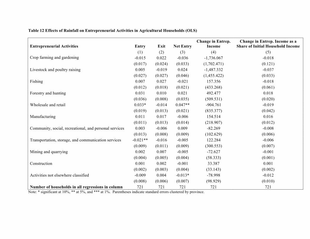
Table 12 Effects of Rainfall on Entrepreneurial Activities in Agricultural Households (OLS)

Entrepreneurial Activities Entry Exit Net Entry Change in Entrep.

Income Change in Entrep. Income as a

Share of Initial Household Income (1) (2) (3) (4) (5)

Crop farming and gardening -0.015 0.022 -0.036 -1,736.067 -0.018 (0.017) (0.024) (0.033) (1,702.471) (0.121) Livestock and poultry raising 0.005 -0.019 0.024 -1,487.332 -0.037 (0.027) (0.027) (0.046) (1,455.422) (0.033) Fishing 0.007 0.027 -0.021 157.356 -0.018 (0.012) (0.018) (0.021) (433.268) (0.061) Forestry and hunting 0.031 0.010 0.021 492.477 0.018 (0.036) (0.008) (0.035) (509.531) (0.020) Wholesale and retail 0.033* -0.014 0.047** -904.761 -0.019 (0.019) (0.013) (0.021) (835.377) (0.042) Manufacturing 0.011 0.017 -0.006 154.514 0.016 (0.011) (0.013) (0.014) (218.907) (0.012) Community, social, recreational, and personal services 0.003 -0.006 0.009 -82.269 -0.008 (0.013) (0.008) (0.009) (102.629) (0.006) Transportation, storage, and communication services -0.021** -0.016 -0.005 122.284 -0.006 (0.009) (0.011) (0.009) (300.553) (0.007) Mining and quarrying 0.002 0.007 -0.005 -72.627 -0.001 (0.004) (0.005) (0.004) (58.333) (0.001) Construction 0.001 0.002 -0.001 33.387 0.001 (0.002) (0.003) (0.004) (33.143) (0.002) Activities not elsewhere classified -0.009 0.004 -0.013* -78.998 -0.012 (0.008) (0.006) (0.007) (98.929) (0.010) Number of households in all regressions in column 721 721 721 721 721

Note: * significant at 10%, ** at 5%, and *** at 1%. Parentheses indicate standard errors clustered by province.

62

Table 13 Effects of Rainfall on Household Labor Supply in Agricultural Households (OLS)

Variables Private

Household Private

Establishment Self

Employed No Pay Government Employer With Pay Total Hours

(1) (2) (3) (4) (5) (6) (7) (8) RF 2006 - RF 2003 -1.338** -2.560 0.014 3.122** 0.051 1.051 0.031 1.506 (1,000 mm.) (0.587) (3.629) (3.810) (1.307) (0.481) (1.027) (0.132) (3.137) Household size 0.670 3.284*** 0.044 0.012 0.656*** 0.970* 0.017 7.297*** (0.487) (0.788) (0.820) (0.579) (0.235) (0.532) (0.044) (1.486) Age -0.046 0.196 0.158 0.204 -0.072 0.057 0.012 0.507 (0.059) (0.206) (0.329) (0.129) (0.060) (0.066) (0.009) (0.432) Education (Elementary omitted) a/

High School -0.875 4.460 1.990 -0.720 1.019* -1.291 -0.261 3.790 (1.192) (3.483) (3.429) (1.939) (0.590) (1.684) (0.245) (4.247) College -1.288* 2.971 1.628 2.060 0.895 -1.026 -0.207 4.696

(0.658) (5.714) (5.867) (2.223) (2.043) (3.229) (0.221) (8.961) Marital Status (Married omitted)

Single b/ -1.700 -3.504 0.527 -0.674 1.051* -1.499 -0.162 -6.569 (1.632) (4.325) (2.519) (2.515) (0.533) (2.062) (0.171) (4.729) Type of Job (Agriculture omitted)

Other Agriculture c/ 0.369 -9.636 -0.041 2.280 0.483 -0.129 0.811 -4.698 (1.179) (5.896) (3.756) (2.639) (0.860) (3.633) (0.682) (7.564) Constant 1.487** 0.396 0.718 -1.317 -0.293 -2.539 0.082 -4.214 (0.665) (2.622) (2.955) (1.455) (0.487) (1.683) (0.176) (4.206) Number of households 721 721 721 721 721 721 721 721 R-squared 0.008 0.032 0.001 0.009 0.025 0.010 0.008 0.055

Notes: * significant at 10%, ** at 5%, and *** at 1%. Parentheses indicate standard errors clustered by province. a/ Elementary includes No Grade Completed. b/ Single includes Widowed, Divorced, and Separated. c/ Other Agriculture refers to agricultural activities other than planting crops, such as farming of animals, animal husbandry, fishing, and logging. d/ Columns 1 to 7 are measured as change in hours worked in different employment types in the week prior to the survey and Column 8 is measured as change in total hours worked by all members (regardless of employment type).

Table 14 Effects of Rainfall on Children’s Labor Supply and Schooling in Agricultural Households (OLS)

Variables Private

Household Private

Establishment Self

Employed No Pay Government Total Hours Schooling

(1) (2) (3) (4) (5) (6) (7) RF 2006 - RF 2003 -0.989 -0.027 0.735 1.308 -0.126 0.775 -0.001 (1,000 mm.) (0.927) (1.233) (0.436) (1.357) (0.139) (1.666) (0.073) Household size 0.339 1.456 -0.008 0.150 0.025 1.986* -0.001 (0.399) (0.979) (0.117) (0.515) (0.024) (1.162) (0.017) Age 0.066 -0.315 0.004 -0.085 -0.009 -0.349 -0.004 (0.054) (0.289) (0.035) (0.107) (0.010) (0.287) (0.006) Education (Elementary omitted) a/

High School -2.311 2.713 1.604* 0.502 -0.215 2.078 0.068 (1.778) (2.168) (0.824) (1.668) (0.210) (3.898) (0.077) College -0.829 0.826 0.605 0.436 -0.181 0.675 0.052

(0.615) (1.408) (0.505) (1.213) (0.196) (2.145) (0.063) Marital Status (Married omitted)

Single b/ -3.666 -5.180 -1.122 0.299 -0.154 -9.977 0.027 (3.222) (6.004) (1.255) (1.047) (0.161) (6.857) (0.170) Type of Job (Agriculture omitted)

Other Agriculture c/ 0.162 -7.468** -0.485 1.259 -0.119 -6.770* -0.048 (0.623) (3.338) (0.439) (1.685) (0.118) (3.406) (0.049) Constant 1.014** 1.586 -0.668 -1.704* 0.275 0.777 0.040 (0.469) (2.098) (0.583) (0.878) (0.271) (2.238) (0.049) Number of households 319 319 319 319 319 319 319 R-squared 0.017 0.042 0.029 0.005 0.004 0.033 0.006

Notes: * significant at 10%, ** at 5%, and *** at 1%. Parentheses indicate standard errors clustered by province. a/ Elementary includes No Grade Completed. b/ Single includes Widowed, Divorced, and Separated. c/ Other Agriculture refers to agricultural activities other than planting crops, such as farming of animals, animal husbandry, fishing, and logging. d/ Columns 1 to 5 are measured as change in hours worked in different employment types in the week prior to the survey and Column 6 is measured as change in total hours worked by all children (regardless of employment type).

Table 15 Effects of Rainfall on Education, Health, and Durable Goods in Agricultural Households (OLS)

Variables Education Health Durable Goods

RF 2006 - RF 2003 0.017*** -0.010** -0.015 (1,000 mm.) (0.005) (0.004) (0.011) Household size 0.006 0.002 0.008 (0.004) (0.002) (0.005) Age -0.000 -0.000 -0.000 (0.000) (0.000) (0.001) Education (Elementary omitted) a/

High School 0.006 0.008 -0.030* (0.007) (0.006) (0.018) College 0.022 -0.009 -0.046*

(0.034) (0.011) (0.025) Marital Status (Married omitted)

Single b/ 0.005 -0.007 -0.014 (0.009) (0.006) (0.010) Type of Job (Agriculture omitted)

Other Agriculture c/ 0.007 -0.007 0.009 (0.013) (0.008) (0.012) Constant 0.004 0.016*** 0.021 (0.006) (0.003) (0.015) Number of households 721 721 721 R-squared 0.022 0.012 0.014

Notes: * significant at 10%, ** at 5%, and *** at 1%. Parentheses indicate standard errors clustered by province. a/ Elementary includes No Grade Completed. b/ Single includes Widowed, Divorced, and Separated. c/ Other Agriculture refers to agricultural activities other than planting crops, such as farming of animals, animal husbandry, fishing, and logging.

Appendix

Effects of Rainfall on Income, Consumption, and Risk-coping Strategies in Rural, Rural Non-Agricultural, Urban, Urban Agricultural, Migrant, and Non-Migrant Households (OLS)

Type of Household

Number of Households Income Consumption

International Remittances

Domestic Transfers Loans

Net Loans

Net Assets

Change in Migration

(1) (2) (3) (4) (5) (6) (7) (8)

Rural Households 1,236 -0.095* -0.080** 0.019 0.033** -0.013** -0.015** -0.004

(0.053) (0.036) (0.035) (0.014) (0.005) (0.006) (0.016) Rural Non-Agriculture 515 -0.074 -0.065 0.077 0.003 -0.007 -0.005 0.013

(0.054) (0.044) (0.077) (0.011) (0.007) (0.008) (0.010)

Urban Households 1,170 0.064 0.004 0.017 -0.009 -0.000 -0.004 0.005

(0.085) (0.053) (0.016) (0.009) (0.003) (0.004) (0.011)

Urban Agricultural 204 0.096 -0.001 0.012 -0.041 -0.006 -0.007 0.016

(0.088) (0.058) (0.062) (0.026) (0.024) (0.026) (0.020)

Migrant 124 0.074 0.011 -0.112 0.175 -0.009 -0.017 -0.018 -0.054

(0.103) (0.047) (0.081) (0.108) (0.018) (0.019) (0.036) (0.074)

Non-Migrant 597 -0.169** -0.147*** -0.028 0.029 -0.015 -0.019* -0.037

(0.067) (0.053) (0.026) (0.024) (0.010) (0.011) (0.038)

Note: Similar regression specification as in agricultural households. * significant at 10%, ** at 5%, and *** at 1%. Parentheses indicate standard errors clustered by

province.