Stanford Exploration Project, Report 103, April 27, 2000

Stanford Exploration Project, Report 103, April 27, 2000, pages 1–352

204

Stanford Exploration Project, Report 103, April 27, 2000, pages 1–352

Transformation of seismic velocity data to extract porosity andsaturation values for rocks

James G. Berryman,1 Patricia A. Berge,2 and Brian P. Bonner3

ABSTRACT

For wave propagation at low frequencies in a porous medium, the Gassmann-Domenicorelations are well-established for homogeneous partial saturation by a liquid. They pro-vide the correct relations for seismic velocities in terms of constituent bulk and shearmoduli, solid and fluid densities, porosity and saturation. It has not been possible, how-ever, to invert these relations easily to determine porosity and saturation when the seismicvelocities are known. Also, the state (or distribution) of saturation, i.e., whether or notliquid and gas are homogeneously mixed in the pore space, is another important variablefor reservoir evaluation. A reliable ability to determine the state of saturation from ve-locity data continues to be problematic. We show how transforming compressional andshear wave velocity data to the ( , )-plane (where and are the parame-ters and is the total density) results in a set of quasi-orthogonal coordinates for porosityand liquid saturation that greatly aids in the interpretation of seismic data for the physicalparameters of most interest. A second transformation of the same data then permits iso-lation of the liquid saturation value, and also provides some direct information about thestate of saturation. By thus replotting the data in the ( , )-plane, inferences can bemade concerning the degree of patchy (inhomogeneous) versus homogeneous saturationthat is present in the region of the medium sampled by the data. Our examples includeigneous and sedimentary rocks, as well as man-made porous materials. These resultshave potential applications in various areas of interest, including petroleum explorationand reservoir characterization, geothermal resource evaluation, environmental restorationmonitoring, and geotechnical site characterization.

INTRODUCTION

In a variety of applied problems, it is important to determine the state of saturation of a porousmedium from acoustic or seismic measurements. In the oil and gas industry, it is commonto use amplitude-versus-offset (AVO) processing of seismic reflection data to reach conclu-sions about the presence of gas, oil, and their relative abundances on the opposite sides of a

1email: [email protected] Livermore National Lab, P. O. Box 808, L-201, Livermore, CA 94550email: [email protected]

3Lawrence Livermore National Lab, P. O. Box 808, L-201, Livermore, CA 94550email: [email protected]

205

206 Berryman et al. SEP–103

reflecting interface underground [e.g., Castagna and Backus (1993)]. For environmental ap-plications, we can expect to be working in the near surface where sensor geometries otherthan surface reflection surveys become practical. For example, when boreholes are present,it is possible to do crosswell seismic tomography, or borehole sonic logging to determine ve-locities [e.g., Harris et al. (1995)]. For AVO processing the data obtained are the seismicimpedances p and s (where is the density, and p, s are the seismic compressional andshear wave velocities, respectively), which arise naturally in reflectance measurements. (Inthis paper, we will use the term “velocities” to refer to measured velocities at seismic, sonic,or ultrasonic frequencies, unless otherwise specified.) However, for crosswell applications,we are more likely to have simply velocity data, i.e., p and s themselves without densityinformation. For well-logging applications, separate measurements of the velocities as well asdensity are possible. Although a great deal of effort has been expended on AVO analysis, rela-tively little has been done to invert the simple velocity data for porosity and saturation. It is ourpurpose to present one method that shows promise for using velocity data to obtain porosityand saturation estimates. The key physical idea used here is the fact that the parameterand the density are the two parameters containing information about saturation, while bothof these together with shear modulus contain information about porosity ( and are de-fined in the next section). These facts are well-known from earlier work of Gassmann (1951),Domenico (1974), and many others. (It is well-established that even though the Gassmann-Domenico relations are derived for the static case, they have been found to describe behaviormeasured in the field at sonic and seismic frequencies, and, in some cases, even in laboratoryultrasonic experiments.) The same facts are used explicitly in AVO analysis (Castagna andBackus, 1993; Ostrander, 1984; Castagna et al., 1985; Foster et al., 1997), but in ways thatare significantly different from those to be described here. A major point of departure is thatthe present work allows direct information to be obtained about, not only the level of the sat-uration, but also concerning the state of saturation, i.e., whether the liquid and gas present aremixed homogeneously, or are instead physically separated and therefore in a state of patchysaturation (Berryman et al., 1988; Endres and Knight, 1989; Knight and Nolen-Hoeksema,1990; Mavko and Nolen-Hoeksema, 1994; Dvorkin and Nur, 1998; Cadoret et al., 1998).Another advantage is that this method uses velocity rather than amplitude information, andtherefore may have less uncertainty and may also require less data processing for some typesof field experiments.

One of the main points of the analysis to be presented is the purposeful avoidance of thewell-known complications that arise at high frequencies, due in large part to velocity disper-sion and attenuation (Biot, 1956a,b; Biot, 1962; O’Connell and Budiansky, 1977; Mavko andNur, 1978; Berryman, 1981; McCann and McCann, 1985; Johnson et al., 1987; Norris, 1993;Best and McCann, 1995). Our point of view is that seismic data (as well as most sonic, andsome ultrasonic data) do not suffer from contamination by the frequency-dependent effects tothe same degree typically seen for high frequency laboratory measurements. By restricting ourrange of frequencies to those most useful in the field, we anticipate a significant simplificationof the analysis and therefore an improvement in our ability to provide both simple and robustinterpretations of field data. In the Discussion section, we also provide a means of identifyingdata in need of correction for dispersion effects.

We introduce the basic physical ideas in the next section. Then we present two new meth-

SEP–103 Extracting porosity & saturation 207

ods of displaying the velocity data. One method is used to sort data points into sets that havesimilar physical attributes, such as porosity. Then, the second method is used to identify boththe level of saturation and the type of saturation, whether homogeneous, patchy, or a combina-tion of the two. We show a subset of the large set of data we have examined that confirms theseconclusions empirically. We then provide some discussion of the results and what we foreseeas possible future applications of the ideas. Finally, we summarize the accomplishments ofthe paper in the concluding section.

ELASTIC AND POROELASTIC WAVE PROPAGATION

For isotropic elastic materials there are two bulk elastic wave speeds (Aki and Richards, 1980),compressional p ( 2 ) and shear s . Here is the overall density, and the

parameters and are the constants that appear in Hooke’s law relating stress to strainin an isotropic material. The constant gives the dependence of shear stress on shear strainin the same direction. The constant gives the dependence of compressional or tensionalstress on extensional or dilatational strains in orthogonal directions. For a porous system withporosity (void volume fraction) in the range 0 1, the overall density of the rock orsediment is just the volume weighted density given by

(1 ) s [S l (1 S) g], (1)

where s , l , g are the densities of the constituent solid, liquid and gas, respectively. S isthe liquid saturation, i.e., the fraction of liquid-filled void space in the range 0 S 1 [seeDomenico (1974)]. When liquid and gas are distributed uniformly in all pores and cracks,Gassmann’s equations say that, for quasistatic isotropic elasticity and low frequency wavepropagation, the shear modulus will be mechanically independent of the properties of anyfluids present in the pores, while the overall bulk modulus K ( 2

3 ) of the rock or sed-iment including the fluid depends in a known way on porosity and elastic properties of thefluid and dry rock or sediment (Gassmann, 1951; Berryman, 1999). Thus, in the Gassmannmodel, the parameter is elastically dependent on fluid properties, while is not. Thedensity also depends on saturation, as shown in equation (1). At low liquid saturations,the bulk modulus of the fluid mixture is dominated by the gas, and therefore the effect of theliquid on is negligible until the porous medium approaches full saturation. This means thatboth velocities p and s will decrease with increasing fluid saturation (Domenico, 1974) dueto the “density effect,” wherein the only quantity changing is the density, which increases inthe denominators of both 2

p and 2s . As the medium approaches full saturation, the shear ve-

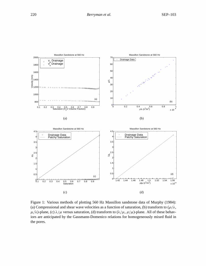
locity continues its downward trend, while the compressional velocity suddenly (over a verynarrow range of saturation values) shoots up to its full saturation value. A well-known ex-ample of this behavior was provided by Murphy (1984). Figure 1 shows how plots of thesedata for sandstones will appear in several choices of display, with Figure 1(a) being one ofthe more common choices. This is the expected (ideal Gassmann-Domenico) behavior of par-tially saturated porous media. The Gassmann-Domenico relations hold for frequencies lowenough (sonic and below) that the solid frame and fluid will move in phase, in response toapplied stress or displacement. The fluid pressure must be (at least approximately) uniform


throughout the porous medium, from which assumption follows the homogeneous saturationrequirement.

PREDICTIONS OF THE THEORY AND EXAMPLES

Gassmann-Domenico relations

Gassmann’s equations (Gassmann, 1951) for fluid substitution state that

K Kdr

2

( ) Km K fand dr , (2)

where Km is the bulk modulus of the single solid mineral, Kdr and dr are the bulk andshear moduli of the drained porous frame. The special combination of moduli defined by

1 Kdr Km is the Biot-Willis parameter (Biot and Willis, 1957). The porosity is ,while K and are the effective bulk and shear moduli of the undrained porous medium that issaturated with a fluid mixture having bulk modulus K f . For partial saturation conditions withhomogeneous mixing of liquid and gas, so that all pores contain the same relative proportionsof liquid and gas, Domenico (1974) among others shows that

1 K f S Kl (1 S) Kg. (3)

The saturation level of liquid is S lying in the range 0 S 1. The bulk moduli are: Kl forthe liquid, and Kg for the gas. When S is small, (3) shows that K f Kg, since Kg Kl . AsS 1, K f remains close to Kg until S closely approaches unity. Then, K f changes rapidly(over a small range of saturations) from Kg to Kl . (Note that the value of Kl may be severalorders of magnitude larger than Kg, as in the case of water and air — 2.25 GPa and 1.45 10 4

GPa, respectively.)

Since has no mechanical dependence on the fluid saturation, it is clear that all the fluiddependence of K 2

3 in (2) resides within the parameter . Other recent work(Berryman et al., 1999) on layered elastic media indicates that should be considered as animportant independent variable for analysis of wave velocities and Gassmann’s results providesome confirmation of this deduction (and furthermore provided a great deal of the motivationfor the present line of research). The parameters K ( 2

3 ) and Kdr ( dr23 dr ) can

be replaced in (2) by and dr without changing the validity of the equation. Thus, like K ,for increasing saturation values, will be almost constant until the porous medium closelyapproaches full saturation.

Now, the first problem that arises with field data is that we usually do not know the reasonwhy data collected at two different locations in the earth differ. It could be that the differencesare all due to the saturation differences we are concentrating on in this paper. Or it couldbe that they are due entirely or only partly to differences in the porous solids that containthe fluids. In fact, solid differences easily can mask any fluid differences because the rangeof detectable solid mechanical behavior is so much greater than that of the fluids (especiallywhen fractures are present).


It is essential to remove such differences due to solid heterogeneity. A related issue con-cerns differences arising due to porosity changes throughout a system of otherwise homoge-neous solids. One way of doing this would be to sort our data into sets having similar poroussolid matrix. For simplicity and because of the types of laboratory data sets available, we willuse porosity here as our material discriminant.

TABLE 1. Monotonicity properties of the parameters and and the density as theporosity and liquid saturation S vary.

Density

S ? S 0 S 0

S S 0 (or 0) S 0 S 0

Considering our three main parameters, , , and , we see that all three depend onporosity, but only and depend on saturation. Using formulas (1)-(3), we can take partialderivatives of each of these expressions first with respect to while holding S constant, andthen with respect to S while holding constant. For now, we are only interested in trendsrather than the exact values, and these are displayed in Table 1. The trend for S 0requires the additional reminder that, although this term is always positive, its value is oftenso small that it may be treated as zero except in the small range of values close to S 1. Also,using Hashin-Shtrikman bounds (Hashin and Shtrikman, 1962) as a guide, it turns out that it isnot possible to make a general statement about the sign of S, since the result dependson the particular material constants. (Related differences of sign are also observed in the datawe show later in this paper; thus, this ambiguity is definitely real and observable.)

Assuming that the primary variables are , , and (further justification of this choice ofprimary variables is provided later in the paper), then the two pieces of velocity data we havecan be used to construct the following three ratios:

2s

2p 2 2

s, (4)

12p 2 2

s, (5)

and

12s

. (6)


We will consider first of all what happens to these ratios for homogeneous mixing of fluids,and then consider the simpler case of ideal patchy saturation, where some pores in the partiallysaturated medium are completely filled with liquid and others are completely dry (or filled withgas).

Homogeneous saturation

For homogeneous saturation, as S varies while porosity remains fixed, the ratio does notchange significantly until S 1. At that point, increases dramatically and thereforedecreases dramatically. Similarly, as S 1, the only changes in over most of the dynamicrange of S are in , which increases linearly with S. Then, when is almost at its maximumvalue, increases dramatically, causing the ratio to decrease dramatically. Thus, doesnot change monotonically with S, but first increases a little and then decreases a lot. Thesetwo ratios may be conveniently compared by plotting data from various rocks and man-madeporous media examples in the ( , )-plane [see Figure 1(b) and Figure 2]. We see that,when data are collected at approximately equal intervals in S, the low saturation points willall cluster together with nearly constant and small increases in , but the final stepsas S 1 lead to major decreases in both ratios. The resulting plots appear as nearly straightlines in this plane, with drained samples plotting to the upper right and fully saturated samplesplotting to the lower left in each of the examples shown in Figure 2. The remaining ratiohas the simplest behavior, since increases monotonically in S, and does not change. So

is a monotonically increasing function of S, and therefore can be considered a usefulproxy of the saturation variable S. [Compare Figures 1(c) and 1(d), and see Figure 3.]

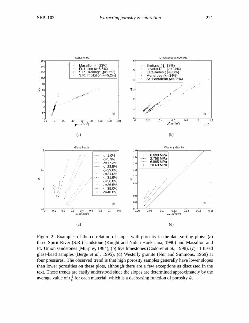
Figure 2(a) includes the same sandstone data from Figure 1, along with other sandstonedata. Similar data for five limestone samples (Cadoret et al., 1998) are plotted in Figure 2(b).The straight line correlation of the data in the sandstone display is clearly reconfirmed by thelimestone data. Numerous other examples of the correlation have been observed. [Fully dryand fully saturated examples are shown here for some of these examples in Figures 2(c) and2(d), for which partial saturation data were unavailable.] No examples of appropriate data forpartially saturated samples have exhibited major deviations from this behavior, although anextensive survey of available data sets has been performed for materials including limestones(Cadoret et al., 1998), sandstones (Murphy, 1984; Knight and Nolen-Hoeksema, 1990), gran-ites (Nur and Simmons, 1969), unconsolidated sands, and some artificial materials such asceramics and glass beads (Berge et al., 1995). This straight line correlation is a very robustfeature of partial saturation data. The mathematical trick that brings about this behavior willnow be explained.

Consider the behavior as increases for fixed S. Two of the parameters ( and ) decreaseas increases, but at different rates, while the third ( ) can have arbitrary variation. [Recall

et al., 1987) that rigorous bounds on the parameters are: 0 K , 0 ,0 , and 2

3 .] To understand the behavior on these plots in Figure 1 aschanges, it will prove convenient to consider polar coordinates (r , ), defined by

r2 42 2

, (7)


and

tan2

, (8)

where is an arbitrary scale factor with dimensions of velocity (chosen so that r is a dimen-sionless radial coordinate for plots like those in Figure 1). Now, if in addition we chooseto be sufficiently large so that s 1 for typical values of s in our data sets, then, usingstandard perturbation expansions, we have

r 2 14s4

12

2 14s

2 4(9)

and

tan 12s2

2s2. (10)

Thus, the angle is well approximated by the ratio in (10), which depends only on the shearvelocity s . We know the shear velocity is a rather weak function of saturation [e.g., Figure1(a)], but a much stronger function of porosity [see, for example, Berge et al. (1995)]. Sowe see that the angle in these plots is most strongly correlated with changes in the porosity.In contrast, the radial position r is principally dependent on the ratio , which we havealready shown to be a strong function of the saturation S, especially in the region close to fullliquid saturation. This analysis shows why the plots in Figures 1(b) and 2 look the way theydo and also why we might be inclined to call these quasi-orthogonal (polar) plots of saturationand porosity. Because of the function these plots play in our analysis, we will call them the“data-sorting” plots.

In contrast, the plots in Figure 3 contain information about fluid spatial distribution, aswill be discussed at greater length later in this paper. The bulk modulus K f contains the onlyS dependence in (2). Thus, for porous materials satisfying Gassmann’s homogeneous fluidconditions and for low enough frequencies, the theory predicts that, if we use velocity datain a two-dimensional plot with one axis being the saturation S and the other being the ratio

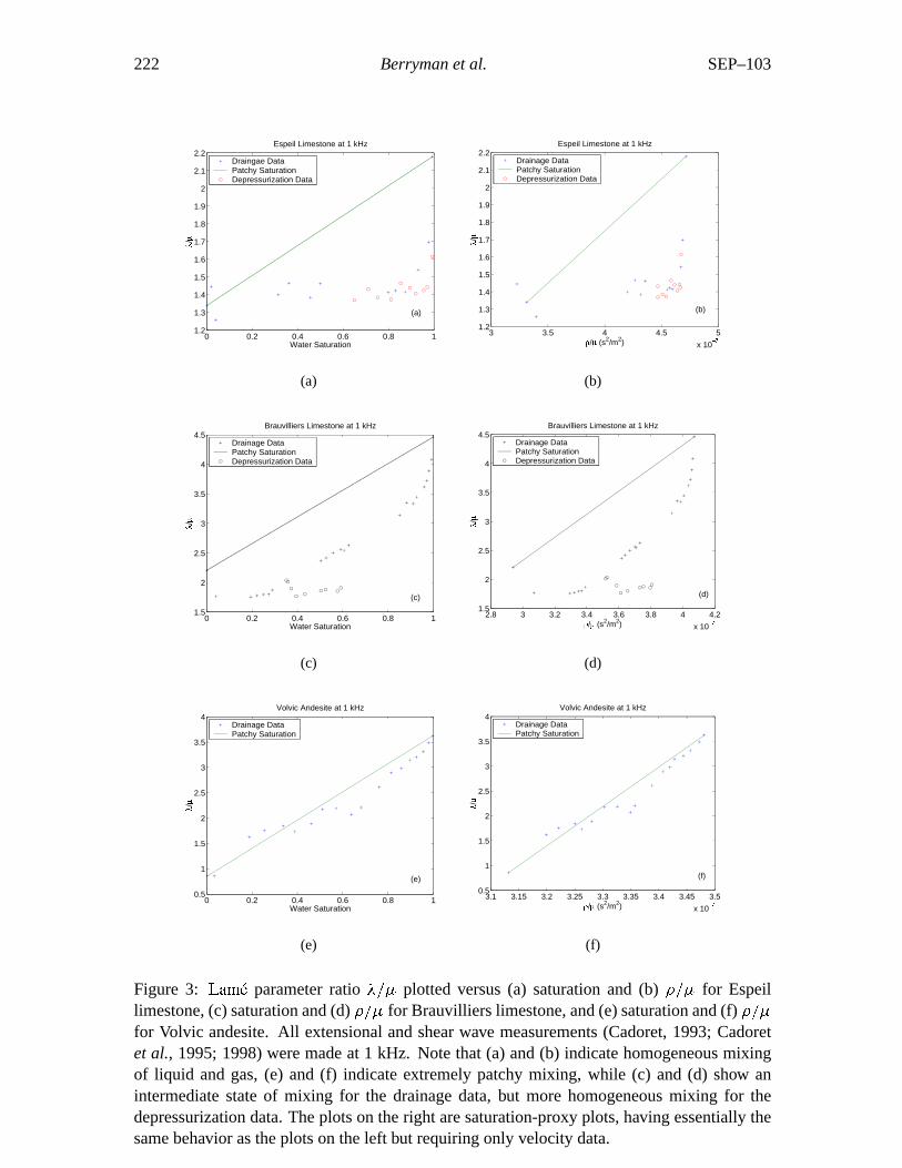
( p s)2 2, then the results will lie along an essentially straight (horizontal) line untilthe saturation reaches S 1 (around 95% or higher), where the curve formed by the data willquickly rise to the value determined by the velocities at full liquid saturation. On such a plot,the drained data appear in the lower left while the fully saturated data appear in the upper right.This behavior is illustrated in Figure 3(a) for Espeil limestone. The behavior of the other plotsin Figure 3 will be described below.

Before leaving this discussion of homogeneous saturation, we should note that there is onelaboratory saturation technique for which it is known — from direct observations (Cadoret etal., 1998) using x-ray imaging — that very homogeneous liquid-gas mixtures will generally beproduced. This method is called “depressurization.” When such data are available (see Figure3), we expect they will always behave according to the Gassmann-Domenico predictions. Incontrast, the more common approach which produces drainage data is less predictable, sincethe manner and rate of drainage depend strongly on details of particular samples — especially


on surface energies that control capillarity and on permeability magnitude and distribution.Thus, the drainage technique can produce homogeneous saturation, or patchy saturation, oranything in between.

Patchy saturation

The preceding analysis centered on homogeneous saturation of porous media. On the otherhand, consider a porous medium containing gas and liquid mixed in a heterogeneous man-ner, so that patches of the medium hold only gas while other patches hold only liquid in thepores. Then, the theory predicts that, depending to some extent on the spatial distribution ofthe patches, the results will deviate overall from Gassmann’s results (although Gassmann’sresults will hold locally in each individual patch). If we consider the most extreme cases ofspatial distribution possible, which are laminated regions of alternating liquid saturation andgas saturation, then the effective bulk modulus will be determined by an average of the twoextreme values of (2): K S 0 Kdr and K S 1. Using saturation as the weighting factor, theharmonic mean and the mean are the two well-known extremes of behavior (Hill, 1952). Ofthese two, the one that differs most from (2) for 0 S 1 is the mean. And, because of K ’slinear dependence on both and , and ’s independence of S, we therefore have

patchy(S) (1 S) dr S S 1. (11)

So, on our plot in the ( , )-plane, the results for the mean will again lie along a straightline, but now the line goes directly from the unsaturated value (S 0) to the fully saturatedvalue (S 1) [e.g., Figure 3(e)]. The two straight lines described [the one given by (11) andthe horizontal one discussed in the preceding paragraph for saturations up to about 95%] arerigorous results of the theory, and form two sides of a triangle that will contain all data forpartially saturated systems, regardless of the type of saturation present. The third side of thistriangle provides a rigorous bound on the behavior as full saturation is approached (it justcorresponds to the physical requirement that S 1, so values with S 1 have no physicalsignificance). In general, heterogeneous fluid distribution can produce points anywhere withinthe resulting triangle, but not outside the triangle (within normal experimental error).

A brief presentation of some examples (Figure 3) will now follow a reminder of an impor-tant and well-known caveat.

Caveats for chemical effects

Some deviations from these conclusions can be expected at the lowest saturations. Chemicaleffects, which have not been accounted for in the mechanical analysis, can and often do leadto the situation that dry and drained (nearly dry or room dry) samples have somewhat differ-ent properties (Bonner et al., 1997). These differences are larger than can be explained bymechanical analyses alone. [For example, see Figures 3(a) and 3(b). Take special note of thethree lowest saturation values in these Figures.] We discuss this point at greater length in theDiscussion section.


Some illustrative examples

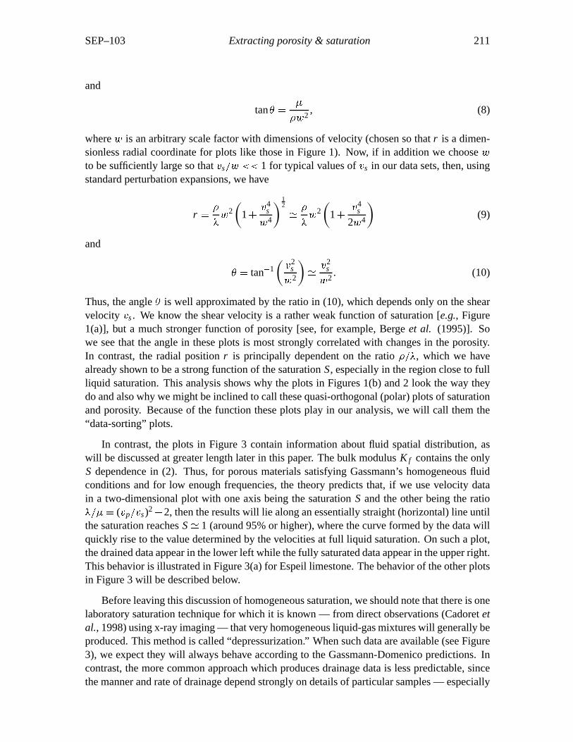
Figure 3 shows three examples of the results obtained with plots in the (S, )-plane andin the ( , )-plane (using as a proxy for S) for two limestones and one andesitefrom laboratory data of Cadoret (1993) and Cadoret et al. (1995; 1998). In Figure 3, the truesaturation data are used in the Figures on the left and the proxy for saturation ( ) is usedon the right. We therefore call the right hand diagrams “saturation-proxy” plots. Using theinterpretations arising for our analysis of Gassmann-Domenico partial-saturation theory, wesee that Figures 3(a) and (b) indicate homogeneous mixing of liquid and gas, while Figures3(e) and (f) indicate extremely patchy mixing, and Figures 3(c) and (d) show an intermediatestate of mixing for the drainage data, but more homogeneous mixing (as expected) for thedepressurization data. The Espeil limestone was observed to be the most dispersive of allthose rocks considered in the data sets of Cadoret (1993) and Carodet et al. (1995; 1998). Sothis case is a very stringent test of the method. In fact, if we were to plot the correspondingdata for Espeil limestone at 500 kHz, we would not find such simple and easily interpretedbehavior on these plots. Our explanation for this difference between the 500 kHz and 1 kHzresults for Espeil limestone is that the dispersion introduces effects not accounted for by thesimple Gassmann-Domenico theory, and that there is then no reason to think that our methodshould work for such high frequencies as 500 kHz. We have found other examples where itdoes work for frequencies higher than one might expect the method to be valid. The point isthat, if we restrict the range of frequencies considered to 1 kHz or less, the method appearsto work quite well on most (and perhaps all) samples. [But, at higher frequencies, the solidand fluid can move out of phase and other relations developed by Biot (1956a,b; 1962) andothers (O’Connell and Budiansky, 1977; Mavko and Nur, 1978; Berryman, 1981; McCannand McCann, 1985; Johnson et al., 1987; Norris, 1993; Best and McCann, 1995) apply.]

DISCUSSION

Rocks containing more than one mineral

The analysis presented here has been limited for simplicity to the case of single mineral porousrocks. In fact the main parts of the analysis do not change in any significant way if the rockhas multiple constituents. The well-known result of Brown and Korringa (1975) states that

K Kdr

2

Ks K K fand dr , (12)

where Ks is the unjacketed bulk modulus of the composite solid frame, K is the unjacketedpore modulus of the composite solid frame, 1 Kdr Ks is the appropriate Biot-Willis(1957) parameter for this situation. The remaining parameters have the same significance asin (2). The functional dependence of Ksat on the saturation S is clearly the same in bothformulas. If we were trying to infer properties of the solid from these formulas, then of course(12) would be more difficult to interpret. But for our present purposes, we are only tryingto infer porosity, saturation values, and saturation state. For these physical parameters, theanalysis goes through without change.


On uniqueness of -diagrams

Since the possible linear combinations of the elastic bulk and shear moduli (K and ) areinfinite, it is natural to ask why (or if) the choice K 2

3 is special? Is there perhaps someother combination of these constants that works as well or even better than the choice madehere? There are some rather esoteric reasons based on recent work (Berryman et al., 1999)in the analysis of layered anisotropic elastic media that lead us to believe that the choice isindeed special, but we will not try to describe these reasons here. Instead we will point outsome general features of the two types of plots that make it clear that this choice is generallygood, even though others might be equally good or even better in special circumstances. First,in the diagram using the ( , )-plane, it is easy to see that any plot of data using linearcombinations of the form ( , ( c ) ), where c is any real constant, will have preciselythe same information and the display will be identical except for a translation of the valuesalong the ordinate by the constant value c. Thus, for example taking c 2

3 , plots of ( ,K ) will have exactly the same interpretational value as those presented here. But, if we nowreconsider the data-sorting plot (e.g., Figure 2) for each of these choices, we need to analyzeplots of the form ( ( c ), ( c )). Is there an optimum choice of the parameter c thatmakes the plots as straight as possible whenever the only variable is the fluid saturation? It isnot hard to see that the class of best choices always lies in the middle of the range of valuesof taken by the data. So setting c 1

2 (min( ) max( )) will always guaranteethat there are very large positive and negative values of ( c ), and therefore that thesedata fall reliably (if somewhat approximately) along a straight line. But the minimum valueof has an absolute minimum of 2

3 , based on the physical requirement of positivity ofK . So c 2

3 is a physical requirement, and since max 23 is a fairly typical value

for porous rocks, it is expected that an optimum value of c 0 will generally be obtainedusing this criterion. Thus, plots based on bulk modulus K instead of will not be as effectivein producing the quasi-orthogonality of porosity and saturation that we have obtained in thedata-sorting style of plotting. We conclude that the choice is not unique (some other choicesmight be as good for special data sets), but it is nevertheless an especially simple choice andis also expected to be quite good for most real data.

Transforming straight lines to straight lines

One important feature concerning connections betweens the points in the two planes ( ,) and ( , ) is the fact that (with only a few exceptions that will be noted) straight

lines in one plane transform into straight lines in the other. For example, points satisfying

A B (13)

in the ( , )-plane (where A and B are constant intercept and slope, respectively), thensatisfy

A 1 A 1 B (14)


in the ( , )-plane. So long as A 0 in (13), the straight line in (13) transforms intothe straight line in (14). This observation is very important because the straight line in (11)corresponds to a straight line in the saturation-proxy plot in the ( , )-plane. But this linetransforms into a straight line in data-sorting plot in the ( , )-plane. In fact the apparentstraight line along which the data align themselves in these plots is just this transformed patchysaturation line.

When A 0 in (13) [which seems to happen rarely if ever in the real data examples, butneeds to be considered in general], the resulting transformed line will just be one of constant

B 1, which is a vertical line on the ( , )-plane. The more interesting specialcase is when B 0, in which situation A or A 1. But this case includes thatof Gassmann-Domenico for homogeneous mixing of the fluids at low to moderate saturationvalues. For B 0, on both planes we have horizontal straight lines, but their lengths can differsignificantly on the two displays.

Interpreting the data point locations

Data points inside the triangle

The triangle described in Section 3.3 provides rigorous bounds on mechanical properties ofporous media. For plots in the ( , )-plane such as those included in Figure 1(d) andFigures 3(b), 3(d), and 3(f), some data points lie between the ideal patchy saturation lineand the Gassmann ideal lower bound. The relative position of the data points may containinformation about the fluid distribution. Consider the case of a core sample that is nearlysaturated, above 90% for example. If the weight of the core is used to determine the saturationbut the core contains a few gas bubbles, the background saturation will be underestimatedand the bubbles themselves represent patches. This is an example of a material having a fewisolated patches contained in an otherwise homogeneous partially-saturated background. Suchdata would plot above but close to the Gassmann curve. In an analogous case for field seismicdata, the background saturation may be known from measurements made at lower frequenciesor in a nearby region, and it may be possible to use such information to determine the relativevolume of patches. For data lying in the middle (i.e., between the bounding curves), someassumptions about fluid distribution could be made and then various estimates about patchyvolumes could be applied to different models such as the Hashin-Shtrikman bounds (Hashinand Shtrikman, 1962) or effective medium theories. Exploration of these issues will be thesubject of future work.

Data points outside the triangle

The sides of the triangle described above set rigorous boundaries for effects associated withhomogeneous saturation and patchy saturation at low frequencies or for situations in whichfrequency-dependent dispersion can be neglected. However, when the data do not in fact sat-isfy these assumptions of the theory, plotting the data this way provides an opportunity toobserve and interpret deviations from the behavior predicted by the theory. For example, data


which plot above the patchy saturation line represent excessively stiff rock. One possible causeof systematically high stiffness values is frequency-dependent dispersion (Biot, 1956a,b; Biot,1962; O’Connell and Budiansky, 1977; Mavko and Nur, 1978; Berryman, 1981; McCannand McCann, 1985; Johnson et al., 1987; Norris, 1993; Best and McCann, 1995). Chemicaleffects, not taken into account in the analysis, might also cause measurements to deviate sys-tematically from predicted behavior. For example, adhesive effects associated with chemicalreactions between pore fluid and solid constituents might cause systematically high values.Another consequence of rock-water interactions is softening of intragranular cements. In thiscase, data for susceptible rocks would systematically plot below the Gassmann line at low sat-urations. Direct indications from elastic data of rock-water interactions [e.g., see Bonner et al.(1997)] may lead to new methods of determining other rock properties controlled by chemicaleffects, such as the tensile strength.

CONCLUSIONS

We have shown that seismic/sonic velocity data can be transformed to polar coordinates thathave quasi-orthogonal dependence on saturation and porosity. This observation is based on theGassmann-Domenico relations, which are known to be valid at low frequencies. The trans-formation loses its effectiveness at high frequencies whenever dispersion becomes significant,because then Biot theory and/or other effects play important roles in determining the velocities.So, the simple relations between p, s , and , , , and S break down at high frequencies. Ourresults are, nevertheless, quite encouraging because the predicted relationships seem to workin many cases up to frequencies of 1 kHz, and in a few special cases to still higher frequencies.These results present a straightforward method for obtaining porosity, saturation, and some in-formation about spatial distribution of fluid (i.e., patchy versus homogeneous) in porous rocksand sediments, from compressional and shear wave velocity data alone. These results have po-tential applications in various areas of interest, including petroleum exploration and reservoircharacterization, geothermal resource evaluation, environmental restoration monitoring, andgeotechnical site characterization. The methods may also provide physical insight suggestingnew approaches to AVO data analysis.

ACKNOWLEDGMENTS

We thank Bill Murphy and Rosemarie Knight for providing access to their unpublished datafiles. We thank Carmen Mora for helpful comments on the text. We thank Norman H. Sleepfor his insight clarifying the significance of our sorting method for plotting seismic data.

REFERENCES

Aki, K., and Richards, P. G., 1980, Quantitative Seismology: Theory and Methods, Vols. I &II, W. H. Freeman and Company, New York.


Berge, P. A., Bonner, B. P., and Berryman, J. G., 1995, Ultrasonic velocity-porosity relation-ships for sandstone analogs made from fused glass beads: Geophysics 60, 108–119.

Berryman, J. G., 1981, Elastic wave propagation in fluid-saturated porous media: J. Acoust.Soc. Am. 69, 416–424.

Berryman, J. G., 1999, Origin of Gassmann’s equations: Geophysics 64, 1627–1629.

Berryman, J. G., Grechka, V. Y., and Berge, P. A., 1999, Analysis of Thomsen parameters forfinely layered VTI media: Geophys. Prospect. 47, 959–978.

Berryman, J. G., Thigpen, L., and Chin, R. C. Y., 1988, Bulk elastic wave propagation inpartially saturated porous solids: J. Acoust. Soc. Am. 84, 360–373.

Best, A. I., and McCann, C., 1995, Seismic attenuation and pore-fluid viscosity in clay-richreservoir sandstones: Geophysics 60, 1386–1397.

Biot, M. A., 1956a, Theory of propagation of elastic waves in a fluid-saturated porous solid. I.Low-frequency range: J. Acoust. Soc. Am. 28, 168–178.

Biot, M. A., 1956b, Theory of propagation of elastic waves in a fluid-saturated porous solid.II. Higher frequency range: J. Acoust. Soc. Am. 28, 179–1791.

Biot, M. A., 1962, Mechanics of deformation and acoustic propagation in porous media: J.Appl. Phys. 33, 1482–1498.

Biot, M. A., and Willis, D. G., 1957, The elastic coefficients of the theory of consolidation: J.Appl. Mech. 24, 594–601.

Bonner, B. P., Hart, D. J., Berge, P. A., and Aracne, C. M., 1997, Influence of chemistryon physical properties: Ultrasonic velocities in mixtures of sand and swelling clay (ab-stract): LLNL report UCRL-JC-128306abs, Eos, Transactions of the American Geophys-ical Union 78, Fall Meeting Supplement, F679.

T., Coussy, O., and Zinzner, B., 1987, Acoustics of Porous Media, Gulf Publishing,Houston, Texas, pp. 56.

Brown, R. J. S., and Korringa, J., 1975, On the dependence of the elastic properties of a porousrock on the compressiblity of the pore fluid: Geophysics 40, 608–616.

Cadoret, T., 1993, Effet de la saturation eau/gaz sur les pr acoustiques des roches,aux sonores et ultrasonores. Ph.D. Dissertation, Univ de Paris VII,

Paris, France.

Cadoret, T., Marion, D., and Zinszner, B., 1995, Influence of frequency and fluid distributionon elastic wave velocities in partially saturated limestones: J. Geophys. Res. 100, 9789–9803.

Cadoret, T., Mavko, G., and Zinszner, B., 1998, Fluid distribution effect on sonic attenuationin partially saturated limestones: Geophysics 63, 154–160.


Castagna, J. P., and Backus, M. M., 1993, Offset-Dependent Reflectivity – Theory and Practiceof AVO Analysis, Society of Exploration Geophysicists, Tulsa, OK.

Castagna, J. P., Batzle, M. L., and Eastwood, R. L., 1985, Relationship between compressional-wave and shear-wave velocities in clastic silicate rocks: Geophysics 50, 571–581.

Domenico, S. N., 1974, Effect of water saturation on seismic reflectivity of sand reservoirsencased in shale: Geophysics 39, 759–769.

Dvorkin, J., and Nur, A., 1998, Acoustic signatures of patchy saturation: Int. J. Solids Struct.35, 4803–4810.

Endres, A. L., and Knight, R., 1989, The effect of microscopic fluid distribution on elasticwave velocities: Log Anal. 30, 437–444.

Foster, D. J., Keys, R. G., and Schmitt, D. P., 1997, Detecting subsurface hydrocarbons withelastic wavefields: Inverse Problems in Wave Propagation, edtied by G. Chavent, G. Pa-panicolaou, P. Sacks, and W. Symes, Springer, New York, pp. 195–218.

Gassmann, F., 1951, die medien: Vierteljahrsschrift der Naturforschen-den Gesellschaft in h, 96, 1–23.

Harris, J. M., Nolen-Hoeksema, R. C., Langan, R. T., Van Schaack, M., Lazaratos, S. K., andRector, J. W., III, 1995, High-resolution crosswell imaging of a west Texas carbonatereservoir: Part 1–Project summary and interpretation: Geophysics 60, 667–681.

Hashin, Z., and Shtrikman, S., 1962, A variational approach to the theory of elastic behaviourof polycrystals: J. Mech. Phys. Solids 10, 343–352.

Hill, R., 1952, The elastic behaviour of crystalline aggregate: Proc. Phys. Soc. London A 65,349–354.

Johnson, D. L., J. Koplik, and R. Dashen, Theory of dynamic permeability and tortuosity influid-saturated porous-media: J. Fluid Mech. 176, 379–402 (1987).

Knight, R., and Nolen-Hoeksema, R., 1990, A laboratory study of the dependence of elasticwave velocities on pore scale fluid distribution: Geophys. Res. Lett. 17, 1529–1532.

Mavko, G., and Nolen-Hoeksema, R., 1994, Estimating seismic velocities at ultrasonic fre-quencies in partially saturated rocks: Geophysics 59, 252–258.

Mavko, G. M., and Nur, A., 1978, The effect of nonelliptical cracks on the compressibility ofrocks: Geophysics 83, 4459–4468.

McCann, C., and McCann, D. M., 1985, A theory of compressional wave attenuation in non-cohesive sediments: Geophysics 50, 1311–1317.

Murphy, William F., III, 1984, Acoustic measures of partial gas saturation in tight sandstones:J. Geophys. Res. 89, 11549–11559.


Norris, A. N., 1993, Low-frequency dispersion and attenuation in partially saturated rocks: J.Acoust. Soc. Am. 94, 359–370.

Nur, A., and Simmons, G., 1969, The effect of saturation on velocity in low porosity rocks:Earth and Planet. Sci. Lett. 7, 183–193.

O’Connell, R. J., and Budiansky, B., 1977, Viscoelastic properties of fluid-saturated crackedsolids: J. Geophys. Res. 82, 5719–5736.

Ostrander, W. J., 1984, Plane-wave reflection coefficients for gas sands at non-normal anglesof incidence: Geophysics 49, 1637–1648.


0.1 0.2 0.3 0.4 0.5 0.6 0.7 0.8 0.9

800

1000

1200

1400

1600

1800

2000Massillon Sandstone at 560 Hz

Saturation (H2O Volume Fraction)

Vel

ocity

(m

/s)

(a)

vp Drainage

vs Drainage

(a)

0 0.2 0.4 0.6 0.8 1

x 10

0

10

20

30

40

50

60

70Massillon Sandstone at 560 Hz

/ (s2/m2)/

(b)

Drainage Data

(b)

0.1 0.2 0.3 0.4 0.5 0.6 0.7 0.8 0.90

0.5

1

1.5

2

2.5

3

3.5

4

4.5Massillon Sandstone at 560 Hz

Saturation

/

(c)

Drainage DataPatchy Saturation

(c)

1.42 1.44 1.46 1.48 1.5 1.52 1.54 1.56

x 10

0

0.5

1

1.5

2

2.5

3

3.5

4

4.5Massillon Sandstone at 560 Hz

/ (s2/m2)

/

(d)

Drainage DataPatchy Saturation

(d)

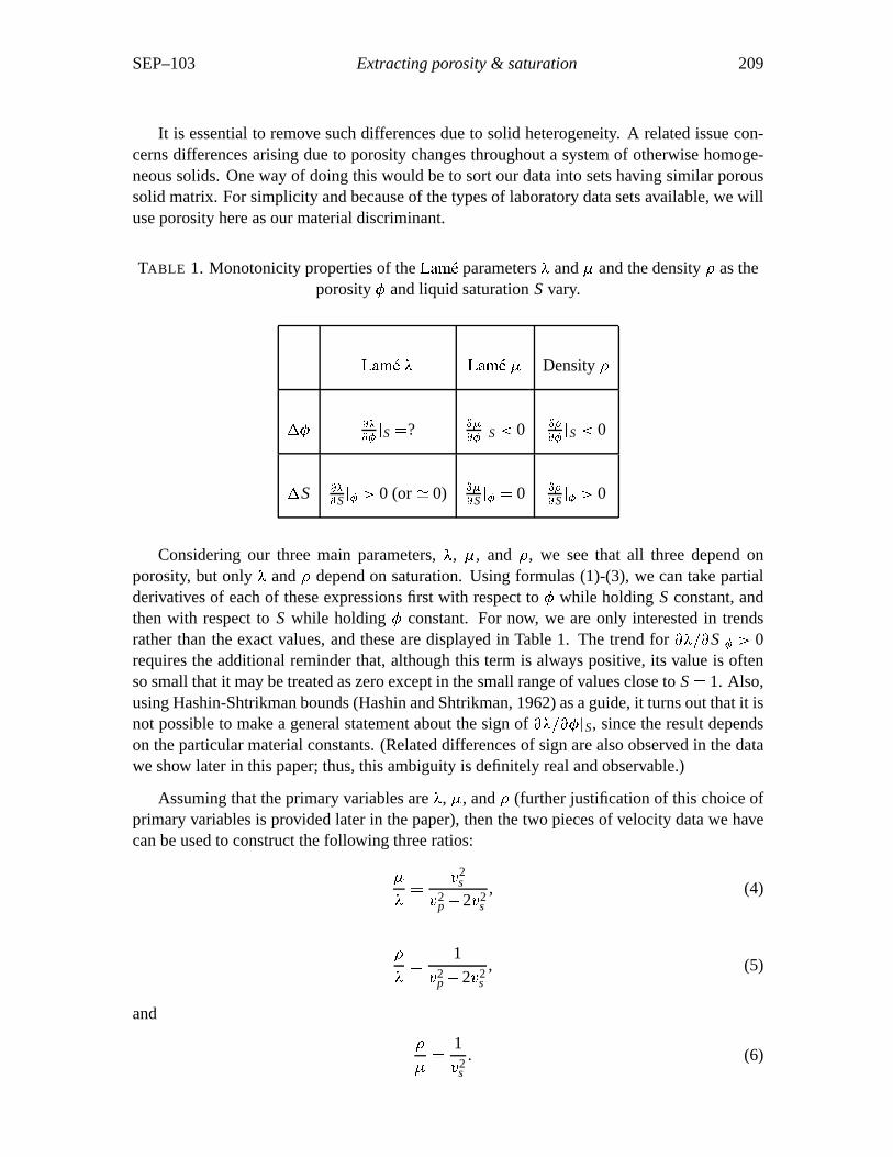
Figure 1: Various methods of plotting 560 Hz Massillon sandstone data of Murphy (1984):(a) Compressional and shear wave velocities as a function of saturation, (b) transform to ( ,

)-plane, (c) versus saturation, (d) transform to ( , )-plane. All of these behav-iors are anticipated by the Gassmann-Domenico relations for homogeneously mixed fluid inthe pores.


0 20 40 60 80 100 120 140

0

20

40

60

80

100

120

140

160Sandstones

/ (s2/km2)

/

(a)

Massillon ( =23%)Ft. Union ( =8.5%)S.R. Drainage ( =5.2%)S.R. Imbibition ( =5.2%)

(a)

0 0.2 0.4 0.6 0.8 1 1.2

x 10

0

1

2

3

4

5

6Limestones at 500 kHz

/ (s2/m2)

/

(b)

Bretigny ( =18%)Lavoux R.F. ( =24%)Estaillades ( =30%)Menerbes ( =34%)St. Pantaleon ( =35%)

(b)

0 0.1 0.2 0.3 0.4 0.5 0.6 0.7 0.80.5

1

1.5

2Glass Beads

/ (s2/km2)

/

(c)

=1.0%=5.9%=17.3%=28.5%=29.0%=31.0%=31.9%=36.0%=36.5%=39.0%=40.0%

(c)

0.06 0.08 0.1 0.12 0.14 0.16 0.180.7

0.8

0.9

1

1.1

1.2

1.3

1.4

1.5

1.6Westerly Granite

/ (s2/km2)

/

(d)

0.690 MPa2.758 MPa6.895 MPa20.69 MPa

(d)

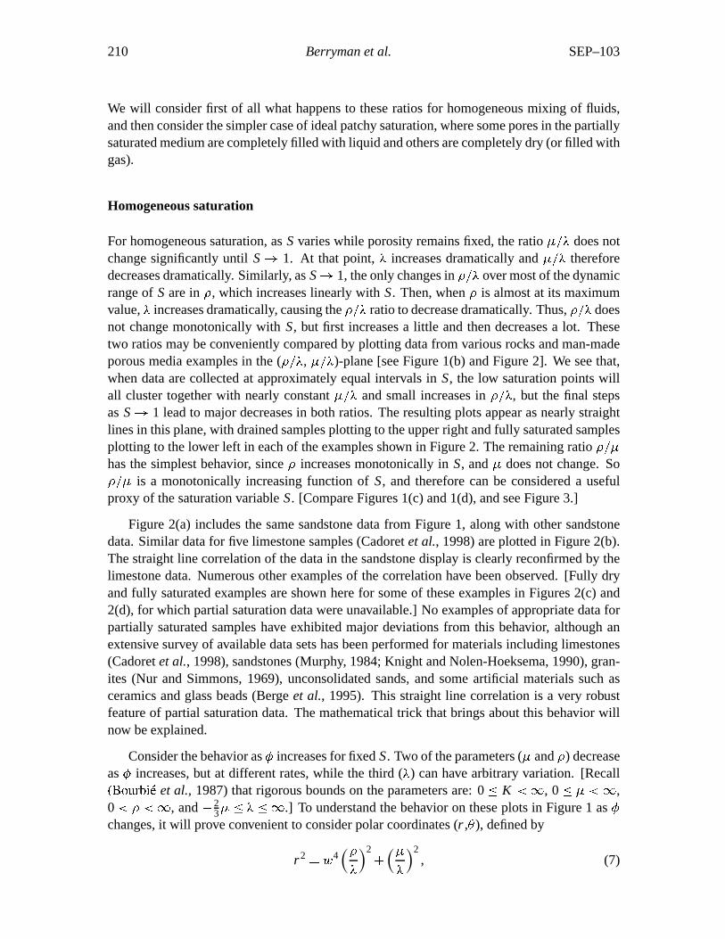
Figure 2: Examples of the correlation of slopes with porosity in the data-sorting plots: (a)three Spirit River (S.R.) sandstone (Knight and Nolen-Hoeksema, 1990) and Massillon andFt. Union sandstones (Murphy, 1984), (b) five limestones (Cadoret et al., 1998), (c) 11 fusedglass-bead samples (Berge et al., 1995), (d) Westerly granite (Nur and Simmons, 1969) atfour pressures. The observed trend is that high porosity samples generally have lower slopesthan lower porosities on these plots, although there are a few exceptions as discussed in thetext. These trends are easily understood since the slopes are determined approximately by theaverage value of 2

s for each material, which is a decreasing function of porosity .


0 0.2 0.4 0.6 0.8 11.2

1.3

1.4

1.5

1.6

1.7

1.8

1.9

2

2.1

2.2

Water Saturation

/

Espeil Limestone at 1 kHz

(a)

Draingae Data Patchy Saturation Depressurization Data

(a)

3 3.5 4 4.5 5

x 10

1.2

1.3

1.4

1.5

1.6

1.7

1.8

1.9

2

2.1

2.2Espeil Limestone at 1 kHz

/ (s2/m2)

/

(b)

Drainage Data Patchy Saturation Depressurization Data

(b)

0 0.2 0.4 0.6 0.8 11.5

2

2.5

3

3.5

4

4.5Brauvilliers Limestone at 1 kHz

Water Saturation

/

(c)


(c)

2.8 3 3.2 3.4 3.6 3.8 4 4.2

x 10

1.5

2

2.5

3

3.5

4

4.5Brauvilliers Limestone at 1 kHz

/

(d)

/ (s2/m2)


(d)

0 0.2 0.4 0.6 0.8 10.5

1

1.5

2

2.5

3

3.5

4Volvic Andesite at 1 kHz

Water Saturation

/

(e)

Drainage Data Patchy Saturation

(e)

3.1 3.15 3.2 3.25 3.3 3.35 3.4 3.45 3.5

x 10

0.5

1

1.5

2

2.5

3

3.5

4Volvic Andesite at 1 kHz

/

/ (s2/m2)

(f)

Drainage Data Patchy Saturation

(f)

Figure 3: parameter ratio plotted versus (a) saturation and (b) for Espeillimestone, (c) saturation and (d) for Brauvilliers limestone, and (e) saturation and (f)for Volvic andesite. All extensional and shear wave measurements (Cadoret, 1993; Cadoretet al., 1995; 1998) were made at 1 kHz. Note that (a) and (b) indicate homogeneous mixingof liquid and gas, (e) and (f) indicate extremely patchy mixing, while (c) and (d) show anintermediate state of mixing for the drainage data, but more homogeneous mixing for thedepressurization data. The plots on the right are saturation-proxy plots, having essentially thesame behavior as the plots on the left but requiring only velocity data.

372 SEP–103

Documents

Stanford Exploration Project, Report 103, April 27, 2000