Standup and Stabilization of the Inverted Pendulum

by

Andrew K. Stimac

Submitted to the Department of Mechanical Engineering in Partial Fulfillment of the Requirements for the Degree of

Bachelor of Science

at the

Massachusetts Institute of Technology

June 1999

© 1999 Andrew K. Stimac

The author hereby grants permission to MIT to reproduce and distribute publicly paper and electronic copies of this thesis document in whole or in part.

Signature of Author: ............................................................................................................ Department of Mechanical Engineering

May 5, 1999

Certified by: ......................................................................................................................... David L. Trumper

Associate Professor of Mechanical Engineering Thesis Supervisor

Accepted by: ........................................................................................................................ Ernest G. Cravalho

Chairman, Undergraduate Thesis Committee Department of Mechanical Engineering

Standup and Stabilization of the Inverted Pendulum

by

Andrew K. Stimac

Submitted to the Department of Mechanical Engineering on May 5, 1999, in Partial Fulfillment of the Requirements for the Degree of

Bachelor of Science in Mechanical Engineering.

Abstract

The inverted pendulum is a common, interesting control problem that involves many basic elements of control theory. This thesis investigates the standup routine and stabilization at the inverted position of a pendulum-cart system. The standup routine uses strategic cart movements to add energy to the system. Stabilization at the inverted position is accomplished through linear state feedback. Methods are implemented using the Matlab Simulink environment, with a dSPACE DSP controller board for interaction with the physical system. Algorithms described in this report were successful and consistently produced the desired results. This report serves as a guide to the current working system and as background information on the inverted pendulum.

Thesis Supervisor: David L. Trumper Title: Associate Professor of Mechanical Engineering

2

Table of Contents

Page 1. Introduction ....................................................................................................... 6

1.1 Purpose ......................................................................................................... 61.2 Project Overview ......................................................................................... 61.3 Organization ................................................................................................. 71.4 Acknowledgements ...................................................................................... 7

2. Pendulum Cart Modeling and Dynamics ........................................................ 82.1 Lagrangian Dynamic Analysis ..................................................................... 82.2 Linearization and Transfer Function Generation ......................................... 122.3 State Space Representation .......................................................................... 17

3. Apparatus ........................................................................................................... 18

4. Controller Design ............................................................................................... 224.1 Linear Control (Pendulum at Upward Vertical) .......................................... 224.2 Standup Routine ........................................................................................... 24

4.2.1 Cart Position Control .......................................................................... 244.2.2 Motion Strategy: A Work Analysis .................................................... 26

5. Simulink Implementation .................................................................................. 335.1 General Simulink Techniques ...................................................................... 335.2 Overview of the Simulink Model ................................................................ 36

5.2.1 Top Level ............................................................................................ 385.2.2 Measurements ..................................................................................... 405.2.3 Filter Bank .......................................................................................... 415.2.4 Input .................................................................................................... 425.2.5 Linear Controller ................................................................................. 435.2.6 Standup Routine .................................................................................. 435.2.7 Controller Select ................................................................................. 535.2.8 Error Processor .................................................................................... 545.2.9 Control Effort ...................................................................................... 55

6. Recommendations .............................................................................................. 56

Appendix A: Matlab Scripts and Function Files ................................................ 57Appendix B: Operating the Pendulum-Cart System ......................................... 60

References ................................................................................................................ 62

3

List of Figures

Page 2.1 Schematic of Pendulum Cart ........................................................................ 82.2 Pole-zero and Bode Diagrams (Pendulum Down) ........................................ 142.3 Pole-zero and Bode Diagrams (Pendulum Up) ............................................. 16

3.1 Pendulum Cart System Block Diagram ........................................................ 183.2 Schematic of Pendulum Cart System ............................................................ 193.3 Photographs of Pendulum Cart ..................................................................... 20

4.1 Resulting LQR Pole Placement ..................................................................... 234.2 Simulated System Response ......................................................................... 234.3 Bode Diagrams of Cart System ..................................................................... 254.4 Lead Controller Design ................................................................................. 254.5 Experimental Bode Plot of the Cart System ................................................. 264.6 Coordinate System and Free Body Diagram of Pendulum Cart System ...... 264.7 Ratio of Work to Acceleration as a Function of Pendulum Angle ............... 284.8 Cart Motion Strategy .................................................................................... 294.9 Cart Position versus Angle for the Pendulum Swinging to the Right ........... 304.10 Pendulum and Cart Motion at Start Angles of 40°, 100°, and 160° ............. 31

5.1 Simulink Model Using Enables Subsystems to Choose an Output .............. 335.2 Multiport Switch Used to Choose an Output ................................................ 345.3 Hold Maximum and Hold Minimum Simulink Constructions ..................... 355.4 Hold Maximum with Reset ........................................................................... 355.5 Tree Diagram of Subsystem Hierarchy ......................................................... 365.6 Top Level Simulink Model ........................................................................... 395.7 Measurements Subsystem ............................................................................. 405.8 Filter Bank Subsystem .................................................................................. 415.9 Input Subsystem ............................................................................................ 425.10 Linear Controller Subsystem ........................................................................ 435.11 Standup Routine Subsystem ......................................................................... 435.12 Position Generation Subsystem .................................................................... 455.13 Swing Sections .............................................................................................. 455.14 Info Subsystem ............................................................................................. 475.15 Hold Max and Hold Min Subsystems ........................................................... 475.16 Amplitude Lookup Subsystem ...................................................................... 485.17 Routine 1 Subsystem .................................................................................... 495.18 Routine 2 Subsystem .................................................................................... 505.19 Routine 3 Subsystem .................................................................................... 525.20 Controller Select Subsystem ......................................................................... 535.21 Error Processor Subsystem ........................................................................... 545.22 Control Effort Subsystem ............................................................................. 55

4

List of Tables

Page 5.1 Subsystem Hierarchy and Function .............................................................. 375.2 Amplitude Lookup Tables ............................................................................ 49

5

1. Introduction

1.1 Purpose

This report explores the standup and stabilization of an inverted pendulum. It contains a theoretical analysis of the system dynamics and control methods, as well as a summary of the apparatus and implementation. There are two purposes of this report: to summarize and explain the methods of controlling this specific pendulum-cart system; and to explore and illustrate in general the inverted pendulum problem.

A major focus of this project was the use of Simulink software for control implementation. Simulink provides a block diagram representation of signal processing methods. Allowing for easy visualization, Simulink facilitates the design of complex control algorithms. While code scripts have been used previously for this project, Simulink provides a more intuitive and organized solution.

1.2 Project Overview

This thesis covers several topics. Primarily, there are two control problems: the standup routine and the stabilization in the inverted position. Also important, however, is the implementation of these control algorithms in the Simulink environment.

The standup routine uses strategic cart movements to gradually add energy to the pendulum. This involves first placing the cart under position control. Then a routine is developed to prescribe the cart’s movement. This movement is such that the cart does work on the pendulum, in a consistent and efficient manner. It is also important to gradually reduce cart movement amplitude so that the standup routine delivers the pendulum to the inverted pendulum position with small angular velocity.

Inverted pendulum stabilization can be accomplished through several methods. This analysis uses state feedback to provide the desired response. Using LQR optimal design tools as a design hangle, the controlled system poles are placed to provide a fast, stable response.

Simulink implementation requires the exploration of specific Simulink techniques. While state feedback control is well suited to the Simulink environment, the standup routine includes some logic that would be more easily represented in a program script. Adaptation to Simulink requires the generation of several information variables that describe the current system state. These variables are the processed with logical operators in order to determine current actions. The Simulink adaptation is slightly complex. However, the Simulink implementation is superior to a script in many areas because routines have little or no preset order, depending primarily on the present system state.

6

1.3 Organization

The sections of this report cover both the theoretical and experimental aspects of this project. Section 2 contains a theoretical discussion of the system dynamics. This analysis is necessary for system modeling, controller design, and for general background understanding of the pendulum-cart system. Section 3 describes the details of the apparatus, including modeling assumptions and specific parameter values. Section 4 explores the controller design, for both standup and stabilization. Stabilization is covered in Section 4.1, and involves linear state feedback methods. Standup is covered in Section 4.2, which explores the strategic cart motion that delivers energy to the pendulum. Section 5 documents the specific Simulink implementation. This section seves as a user’s guide to the current functioning system, as well as a tutorial on Simulink methods. Finally, Section 6 gives Recommendations for further improvements. Appendix A includes the Matlab files used and Appendix B contains simple instructions on how to operate the system.

1.4 Acknowledgments

I would like to voice my appreciation to everyone who helped me on this project. Special thanks to Professor Trumper for suggesting this thesis and for his guidance along the way, to Mike Liebman for his assistance and support in the Mechatronics Lab, and to Steve Ludwick for sharing his understanding of the current project setup. Finally, many thanks to those who made contributions on this project before me, particularly Steve Ludwick, Ming-chih Weng, and Pradeep Subrahmanyan, and Professor Will Durfee and his students who originally built the pendulum-cart experiment hardware at MIT.

7

2. Pendulum Cart Modeling and Dynamics

For the purpose of this report, it is necessary to understand the dynamics of the pendulum cart system. In the follow pages, a theoretical analysis is conducted, using the Lagrangian approach to derive the state equations. The result is linearized around two points of operation, pendulum up and down, and transfer functions are derived and analyzed. This approach provides an in depth theoretical explanation for the dynamics of this system. Throughout this analysis, vector and matrix quantities are distinguished using bold text.

2.1 Lagrangian Dynamic Analysis

A complete theoretical model of the pendulum cart system can be done using Lagrangian Dynamics. First we choose generalized coordinates, and then derive expressions for the generalized forces, energy functions, and Lagrangian. Finally, we can use Lagrange’s Equation to derive the equations of motion [3].

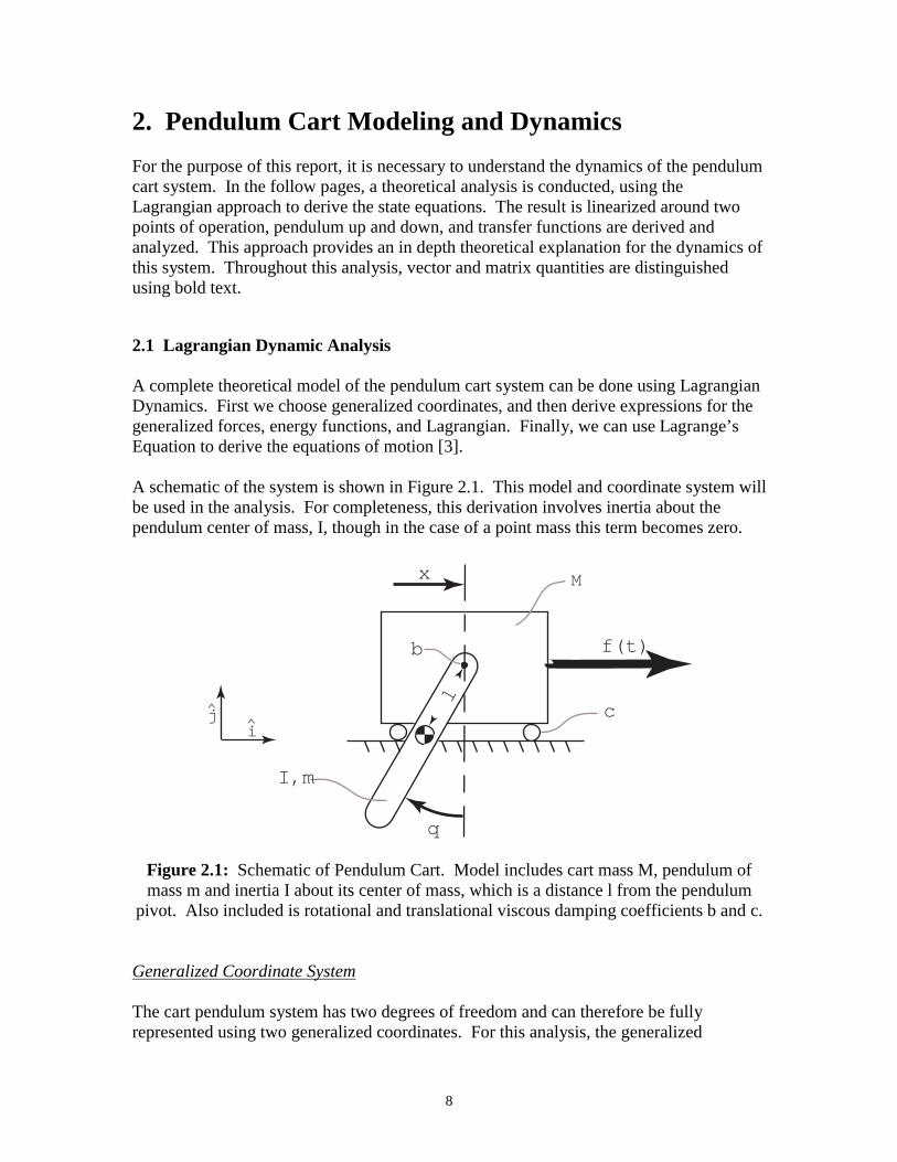
A schematic of the system is shown in Figure 2.1. This model and coordinate system will be used in the analysis. For completeness, this derivation involves inertia about the pendulum center of mass, I, though in the case of a point mass this term becomes zero.

q

x

f(t)

l

I,m

M

b

c i ^

j

Figure 2.1: Schematic of Pendulum Cart. Model includes cart mass M, pendulum of mass m and inertia I about its center of mass, which is a distance l from the pendulum

pivot. Also included is rotational and translational viscous damping coefficients b and c.

Generalized Coordinate System

The cart pendulum system has two degrees of freedom and can therefore be fully represented using two generalized coordinates. For this analysis, the generalized

8

coordinates are chosen as the horizontal displacement of the cart, x, and the rotational displacement of the pendulum, θ :

ξ j : x,θ (2.1)

The positive direction of x is to the right and the positive direction of θ is clockwise, measured from the downward position. Positive θ was chosen in the clockwise direction so that x and θ are both measured to the right when the pendulum is in its inverted position. A complete and indepentent set of the associated admissible variations is given by

ξ j : δ x,δθ (2.2)

so the system is holonomic.

Generalized Forces

An expression for the generalized forces, Ξ j, can be derived from the nonconservative work, given by

W N n

nc ncδ = ∑ f • δ Ri = ∑Ξ δξ j (2.3)j i= 1 j= 1

where Ri is the position vector where the ith nonconservative force acts. The nonconservative forces in this case result from the input force and the system damping,

W nc b&δ = t f x & δθθ − δ (2.4)) ( − δ x xc

Comparing Equations 2.3 and 2.4 yields expressions for the generalized forces:

) ( − xc &Ξ = t f x (2.5)

b&Ξθ θ − =

Kinetic and Potential Energy Functions

The kinetic coenergy function for the cart mass is simply

*TM = 1 xM &2

(2.6)2

9

For the pendulum, the coenergy function can be derived from

1 2T * = 1 m v • v + I ω (2.7)m 2 c c 2

where I is the moment of inertial around the pendulum’s center of mass and vc is the velocity of the pendulum’s center of mass. This velocity can be related to the position of the pendulum’s center of mass,

r = (x − l ) sin ˆ − l cosθ j (2.8)θ ic

by

v = d rc = (x & − l cos θ θ &)i + l sin θ θ & j (2.9)c dt

The angular velocity of the pendulum is simply

&ω θ = (2.10)

Substituting Equations 2.9 and 2.10 into Equation 2.7 yields

& & 2 2 & 2T * = 1 m (x &2 − 2 lx cos + θ θ l cos θ θ + l 2 sin2 θ θ & 2 ) + 1

I θ & 2 (2.11)m 2 2

which, upon simplifying, becomes

& & 2 & 2T * = 1 m (x &2 − 2 lx cos + θ θ l θ ) + 1

I θ & 2 (2.12)m 2 2

The total kinetic coenergy is

T * * & & 2 & 2= TM + T * = 1 Mx&2 + 1

m (x &2 − 2 lx cos + θ θ l θ ) + 1 I θ & 2

(2.13)m 2 2 2

Since the cart moves only in the horizontal direction, the potential energy of the system is determined entirely by the angle of the pendulum, given by

V = − mgl cosθ (2.14)

10

Lagrangian

From the kinetic coenergy and potential energy functions, the Lagrangian is given by

L = T * − V (2.15)

Using Equations 2.13 and 2.14, the Lagrangian can be written as

2( & 2 − 2 lx cos + θθ l θ ) + 1 Iθ & 2 + mglcosθ (2.16)L = 1

xM &2 + 1 x m & & 2 &

2 2 2

Lagrange’s Equation

State equations can be generated using Lagrange’s Equation:

d ⎛ ∂ L ⎞⎟ ∂ L = Ξ j (2.17)dt ⎜

⎜∂ξ & j

⎟ − ∂ξ j⎝ ⎠

The equation for x is

d ⎛ ∂ L ⎞ ∂ L⎜ ⎟ − = Ξ x (2.18)

dt ⎝ ∂ x& ⎠ ∂ x

Using Equation 2.16 and evaluating the partial derivatives yields

d & ) ( − xc & (2.19)( xM & + xm & − mlcos θθ ) − 0 = t f dt

which reduces to

2(M + x m && & ) ( − xc & (2.20)) && − mlcos + θθ mlsin θθ = t f

The equation for θ is

d ⎛ ∂ L ⎞ ∂ L⎜ & ⎟ − = Ξθ (2.21)

dt ⎝ θ∂ ⎠ θ ∂

Using Equation 2.16 and evaluating the partial derivatives yields

d 2 & & & θ &(− xml & cos + θ ml + θ Iθ ) − ( xml & sin − θθ mgl ) sin = − bθ (2.22)dt

11

which reduces to

&& & & b&(ml2 + I) − θ xml && cos + θ xml & sin − θ θ xml & sin − θ θ mglsin = θ θ − (2.23)

Simplifying and rearranging, the system state equations are

&& & 2 ) ( ⎪ ) && + xc & − mlcos + θ θ mlsin θ θ = t f ⎧ (M + x m (2.24)⎨ 2 && &⎪− xml && cos + θ (ml + I) + θ b + θ mglsin = θ 0⎩

2.2 Linearization and Transfer Function Generation

Before proceeding with further analysis, we must linearize the state equations. There are two equilibrium points: θ =0 (pendulum down, stable) and θ =π (pendulum up, unstable). Focusing on small variations of θ about the equilibrium point θ o:

θ = θ 0 ε + (2.25)

& ε = θ &

From a Taylor Series expansion, a first order approximation of any function of θ is

dff ) ( ≈ f (θ ) ε + (2.26)θ 0 dθ θ 0

Also, because higher order terms are neglected,

ε & 2 ≈ 0 (2.27)

2.2.1 Pendulum Down (θ =0)

For θ =0, Equation 2.26 yields to first order

)]0sin( [ = 1cos ≈ θ )0cos( − θ +sin ≈ θ )0sin( θ + )]0[cos( θ =

(2.28)

Substituting these linearizations into the system state equations (Equation 2.24) and neglecting the higher order term yields

⎪ ) && + xc & − ml = θ t f ⎧ (M + x m && ) ( (2.29)⎨ 2 && &⎪− xml && + (ml + I) + θ b + θ mgl = θ 0⎩

12

Taking the Laplace Transform

2⎧(M + s m s X ) ( − mls Θ ) ( = s F ⎪ ) 2 ) ( + s csX s ) ( (2.30)

⎪− s X mls ) 2 s s s ⎨ 2 ) ( + (ml2 + s I Θ ) ( + bsΘ ) ( + mglΘ ) ( = 0⎩

Using substitution to eliminate either X(s) or Θ(s) yields two transfer functions:

) ( = s a 2 + s a + a0s X 2 1sG ) ( =1 ) ( s b 4 + s b 3 + s b 2 + s b s F 4 3 2 1

Θ ) ( = s c (2.31)

G ) ( = s 2s2 ) ( s b 3 + s b 2 + s b + b1s F 4 3 2

where

2a2 = ml2 + I ≈ ml

a1 = b

a2 = mgl2 2 2b4 = (M + m)(ml2 + I) − l m ≈ Mml

) 2b3 = (M + b m + (ml2 + c I ≈ (M + b m + c ml ) )

)= (M + mgl m + bcb2

= mglcb1

c2 = ml

The approximations shown in the coefficients above are for I=0, which is the ideal case where the pendulum is constructed from a point mass and massless rod, so that it has no moment of inertia about its center of mass. Using this approximation, the transfer functions reduce to:

s X 2) ( = s ml 2 + bs + mglsG ) ( = 1 s F 2 ) 2 ] ) ]) ( s Mml 4 + [(M + b m + s c ml 3 + [(M + mgl m + s bc 2 + mglcs

sΘ ) ( = mls (2.32)

sG2 ) ( =s F 2 ) 2 ] ) ]) ( s Mml 3 +[(M + b m + s c ml 2 + [(M + mgl m + s bc + mglc

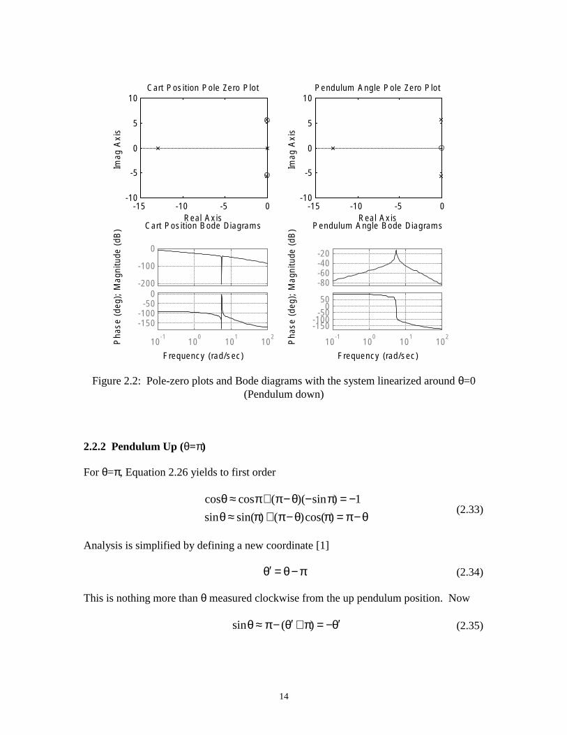
The pole-zero plots and bode diagrams for these transfer functions are shown in Figure 2.2.

13

Cart Position Pole Zero Plot Pendulum Angle Pole Zero Plot

-10

-5

0

5

10

is

-5

0

5

10

is

Imag

Ax

-10

Imag

Ax

-15 -10 -5 0 -15 -10 -5 0 Real Axis Real Axis

Cart Position Bode Di Pendulum Angle Bode Diagrams agrams

Pha

se (

deg)

; M

agni

tude

(dB

)

Pha

se (

deg)

; M

agni

tude

(dB

)

0

-100

-200 0

-50 -100 -150

-20 -40 -60 -80

50 0

-50-100 -150

-1 0 1 2 -1 0 1 21010 10 10 10 10 10 10

Frequency (rad/sec) Frequency (rad/sec)

Figure 2.2: Pole-zero plots and Bode diagrams with the system linearized around θ =0 (Pendulum down)

2.2.2 Pendulum Up (θ =π )

For θ =π , Equation 2.26 yields to first order

− πcos ≈ θ cos + π ( θ − π ) sin )( − = 1

+ π ( θ − π ) cos( ) θ − π = (2.33)

sin ≈ θ ) sin( π

Analysis is simplified by defining a new coordinate [1]

θ′ π − θ = (2.34)

This is nothing more than θ measured clockwise from the up pendulum position. Now

′sin − π ≈ θ ( π + θ ) − = θ′ (2.35)

14

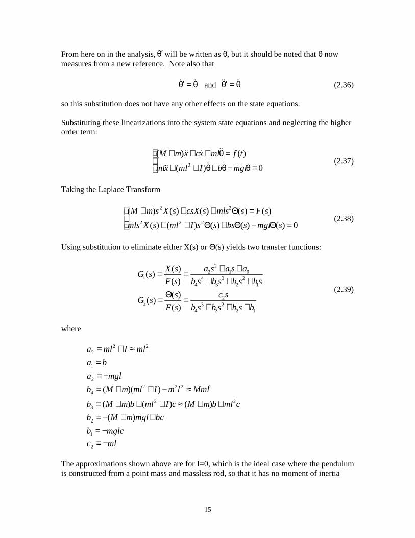
From here on in the analysis, θ′ will be written as θ , but it should be noted that θ now measures from a new reference. Note also that

& & && && θ′ θ = and θ′ θ = (2.36)

so this substitution does not have any other effects on the state equations.

Substituting these linearizations into the system state equations and neglecting the higher order term:

⎪ ) && + xc & + ml = θ t f ⎧ (M + x m && ) ( (2.37)⎨ 2 && &⎪ xml && + (ml + I) + θ b − θ mgl = θ 0⎩

Taking the Laplace Transform

2⎧ (M + s m s X ) ( + mls Θ ) ( = s F ⎪ ) 2 ) ( + s csX s ) ( (2.38)

⎪ s X mls ) 2 s s s ⎨ 2 ) ( + (ml2 + s I Θ ) ( + bsΘ ) ( − mglΘ ) ( = 0⎩

Using substitution to eliminate either X(s) or Θ (s) yields two transfer functions:

) ( = s a 2 + s a + a0s X 2 1sG ) ( =1 ) ( s b 4 + s b 3 + s b 2 + s b s F 4 3 2 1

Θ ) ( = s c (2.39)

G ) ( = s 2s2 ) ( s b 3 + s b 2 + s b + b1s F 4 3 2

where

2a2 = ml2 + I ≈ ml

a1 = b

a2 − = mgl2 2 2b4 = (M + m)(ml2 + I) − l m ≈ Mml

) 2b3 = (M + b m + (ml2 + c I ≈ (M + b m + c ml ) )

)− = (M + mgl m + bcb2

− = mglcb1

c2 − = ml

The approximations shown above are for I=0, which is the ideal case where the pendulum is constructed from a point mass and massless rod, so that it has no moment of inertia

15

about its center of mass. Using this approximation, the transfer functions reduce to:

s X 2) ( = s ml 2 + bs − mglsG ) ( = 1 s F 2 ) 2 ] ( [ M + mgl m + s bc 2 − mglcs) ( ( s Mml 4 + [(M + b m + s c ml 3 − + ) ]

sΘ ) ( = − mls (2.40)

sG2 ) ( = s F 2 ) 2 ] ( [ M + mgl m + s bc − mglc) ( s Mml 3 + [(M + b m + s c ml 2 − + ) ]

The pole-zero plots and bode diagrams for these transfer functions are shown in Figure 2.3.

Cart Position Pole Zero Plot Pendulum Angle Pole Zero Plot

-1

0

1

is

-1

0

1

is

-0.5

0.5

Imag

Ax

-0.5

0.5 Im

ag A

x

-20 -10 0 10 -20 -10 0 10 Real Axis Real Axis

Cart Position Bode Di Pendulum Angle Bode Diagrams agrams

Pha

se (

deg)

; M

agni

tude

(dB

)

Pha

se (

deg)

; M

agni

tude

(dB

)

-20 -40 -60 -80

-100

-150

-60

-80

80 60 40 20

-1 0 1 2 -1 0 1 21010 10 10 10 10 10 10

Frequency (rad/sec) Frequency (rad/sec)

Figure 2.3: Pole-zero plots and Bode diagrams with the system linearized around θ =π (Pendulum up).

16

2.3 State Space Representation

For linear state control of the inverted pendulum, it is necessary to convert the state equations to state space representation in the form

x& =Ax+Bu (2.41)

For the state vector x a change in variable notation is needed, defined by

x =

⎜

⎛⎜⎜⎜⎜ ⎝ ⎟ ⎜

⎛⎜⎜⎜⎜ ⎝

⎞⎟⎟⎟⎟ ⎠ & ⎟

⎞⎟⎟⎟⎟ ⎠θ

x1 x

x&x2 = (2.42)θx3

x4

Referring back to the linearized state equations for Pendulum Up (Equation 2.37), and neglecting I, this change of variables leads to

(

xml &2

⎧⎨⎩

)x m 2 ) ( t f M xml &4 =&+ +cx2 +(2.43)2 −mglx3 =0x ml &4 bx4+ +

From the variable definitions:

x&1

x&3

==

x2 (2.44)

x4

Expressions for x&2 and x&4 can be found by using substitution to eliminate

either x&4 or x&2 from Equation 2.43. The result, in matrix form, is given by

d

dt

⎛⎜⎜⎜⎜ ⎝⎜

x1

x2

x3

x4

⎞⎟⎟⎟⎟ ⎠⎟

=

⎛⎜⎜⎜⎜ ⎝⎦⎜

x1

x2

x3

x4

⎞⎟⎟⎟⎟ ⎠⎟

+

⎡⎢⎢⎢⎢⎣

0

0

0

0 c

⎤ ⎡ ⎤1 0 0 0 ⎥⎥⎥⎥

⎢⎢⎢⎢⎣

⎥⎥⎥⎥⎦1/ Ml

− /M − / /M mg Ml b 1/Mc t f ) ( (2.45)0 0 1 0

2M + ) / Ml g m −(M+ −/ ( ) / Mml b m Ml

17

3. Apparatus

A real pendulum-cart system was used for this thesis project. This system includes the necessary equipment to constrain motion, apply force, measure states, and implement control schemes.

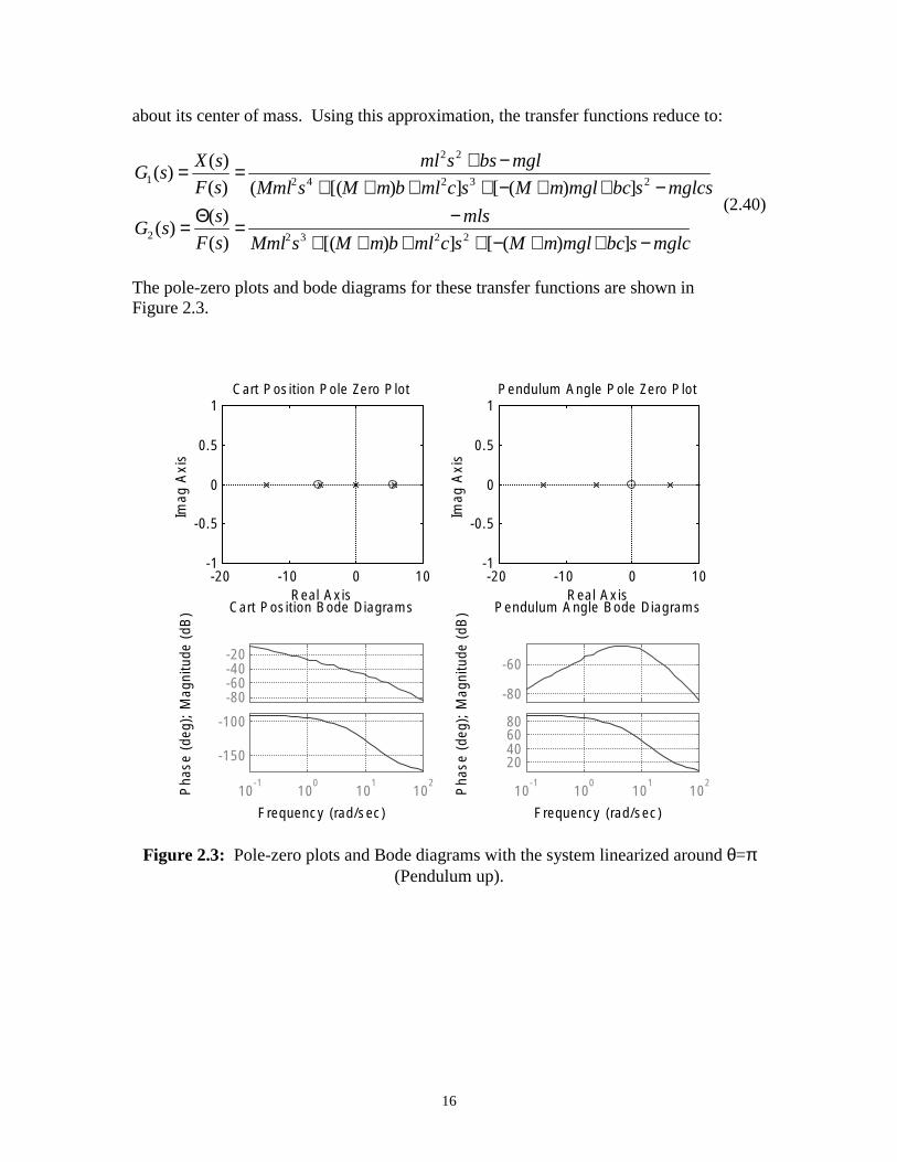
A block diagram of the system is shown in Figure 3.1, with a full schematic in Figure 3.2. The components involved are a current amplifier, DC motor with gearing, a cart with pendulum, an array of feedback instruments, and a computer with Simulink software for signal processing.

Motor Input Output Controller Current

Amplifier Pendulum

Cart

Calibration Sensors

Simulink

Figure 3.1: Pendulum Cart System Block Diagram.

Current is amplified using an Aerotech 4020 DC Servo Controller in current mode. This amplifier has a gain of 2 A/V, with a bandwidth of 2 kHz. Maximum ratings at 25° C are 40 V, 5 A continuous, and 20 A peak (2 seconds). The amplifier input power required is 100-125 V at 50-60 Hz, which is taken directly from an electrical outlet. For general operation, amplifier dynamics are negligible and the amplifier is modeled as a single gain Ka=2 A/V.

The driving motor is an Aerotech Permanent Magnet DC Servo Motor, Model 1135 Standard. The motor has a torque constant Kt=0.17 N-m/A, inertia J=3.6×10-4 kg-m2, and viscous damping b=0.007 N-m/krpm. Because this motor is driven by a current amplifier, the back emf, Kb=18.2 V/krpm, need not be considered. Electrical dynamics can also because of the current drive. In any case, the electrical time constant is τe=2.2 ms, which is small compared to the mechanical time constant of τm=16 ms. Armature resistance, 1.4 Ω, is not important because a current drive is used. The motor torque is connected directly to the cart using a chain drive with a radius of 4 cm. Including this gearing, the total motor gain can be expressed as Km=4.25 N/A. Motor inertia and damping is lumped with parameters of the pendulum cart. This motor is also equipped with a tachometer with constant Ktach=3 V/krpm, used for cart velocity feedback.

18

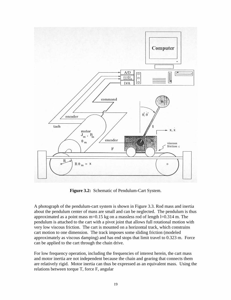
Figure 3.2: Schematic of Pendulum-Cart System.

A photograph of the pendulum-cart system is shown in Figure 3.3. Rod mass and inertia about the pendulum center of mass are small and can be neglected. The pendulum is thus approximated as a point mass m=0.15 kg on a massless rod of length l=0.314 m. The pendulum is attached to the cart with a pivot joint that allows full rotational motion with very low viscous friction. The cart is mounted on a horizontal track, which constrains cart motion to one dimension. The track imposes some sliding friction (modeled approximately as viscous damping) and has end stops that limit travel to 0.323 m. Force can be applied to the cart through the chain drive.

For low frequency operation, including the frequencies of interest herein, the cart mass and motor inertia are not independent because the chain and gearing that connects them are relatively rigid. Motor inertia can thus be expressed as an equivalent mass. Using the relations between torque T, force F, angular

19

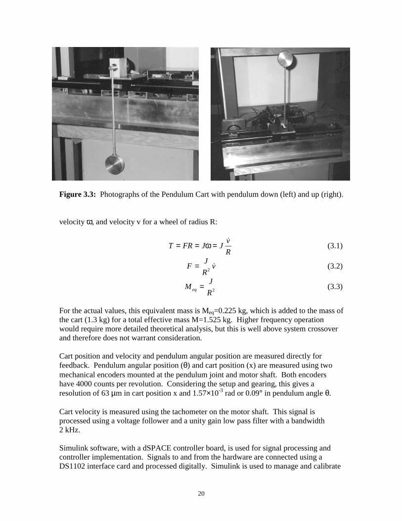
Figure 3.3: Photographs of the Pendulum Cart with pendulum down (left) and up (right).

velocity ω , and velocity v for a wheel of radius R:

v& T = FR = J = ω & J (3.1)

R J

F = v& (3.2)R2

JM = (3.3)eq R2

For the actual values, this equivalent mass is Meq=0.225 kg, which is added to the mass of the cart (1.3 kg) for a total effective mass M=1.525 kg. Higher frequency operation would require more detailed theoretical analysis, but this is well above system crossover and therefore does not warrant consideration.

Cart position and velocity and pendulum angular position are measured directly for feedback. Pendulum angular position (θ ) and cart position (x) are measured using two mechanical encoders mounted at the pendulum joint and motor shaft. Both encoders have 4000 counts per revolution. Considering the setup and gearing, this gives a resolution of 63 µ m in cart position x and 1.57× 10-3 rad or 0.09° in pendulum angle θ .

Cart velocity is measured using the tachometer on the motor shaft. This signal is processed using a voltage follower and a unity gain low pass filter with a bandwidth 2 kHz.

Simulink software, with a dSPACE controller board, is used for signal processing and controller implementation. Signals to and from the hardware are connected using a DS1102 interface card and processed digitally. Simulink is used to manage and calibrate

20

the array of feedback signals, and to implement both the standup routine and linear controller. The sampling rate as implemented was 2000 Hz, which is high enough to produce negligible phase loss at crossover.

21

4. Controller Design

Control algorithms for this project had two functions: 1) to gradually swing the pendulum to the inverted position and then 2) to balance the pendulum at this unstable equilibrium point. The first requires a routine of precision cart movement that gradually adds energy to the system. The second is solved using state feedback. This section focuses on both the theoretical design and experimental results, as these topics are frequently inseparable in controller design. The specific Simulink implementation is covered later in section 5.

4.1 Linear Control (Pendulum Inverted)

In the inverted position, the pendulum is unstable without control. The transfer function between cart position x and control input contains both a pole and a zero in the right half plane. Because of the proximity of this pole zero pair, it is difficult to obtain a stable response through classical feedback methods.

Instead, stabilization of the pendulum is conducted through full state feedback. Using this method, the system poles can be placed arbitrarily.

For a Linear Time Invariant System

x& = Ax + Bu (4.1)

the system poles are given by the eigenvalues of A, defined as the solutions λ to

− λ AI = 0 (4.2)

where I is the identity matrix of proper dimension and the symbol ‘| |’ refers to the matrix determinant. An array of negative feedback gains is used, so that the input u is proportional to the given states:

u − = x (k + k 2x + L+ k x ) − = Kx (4.3)1 1 2 n n

where

K = [k L k ] (4.4)1 k 2 n

For systems with single inputs, u and k1 through kn reduce to scalar quantities, and K is a row vector. Substituting Equation 4.3 into Equation 4.1,

)x& = Ax − BKx = (A − x BK (4.5)

22

-5

0

5

10

15

Imag

inar

y A

xis

Analysis is simplified by defining the controlled state matrix

A = A − BK (4.6)c

yielding

x& = x A (4.7)c

Now the system poles are given by the eigenvalues of Ac, defined by

− λ ACI = 0 (4.8)

It can be shown for most systems that by choosing the proper gain matrix, theeigenvalues of Ac, which are the controlled system poles, can in theory be placedanywhere. Using this method, a fast, stable response can be accomplished.

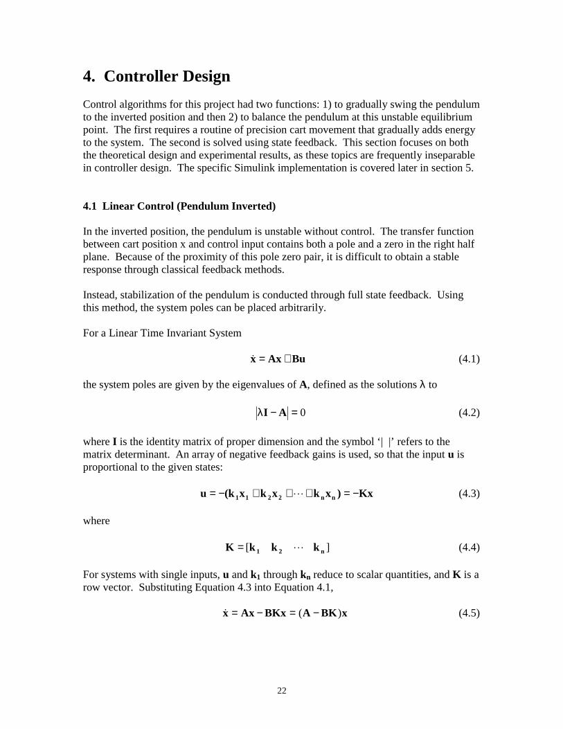
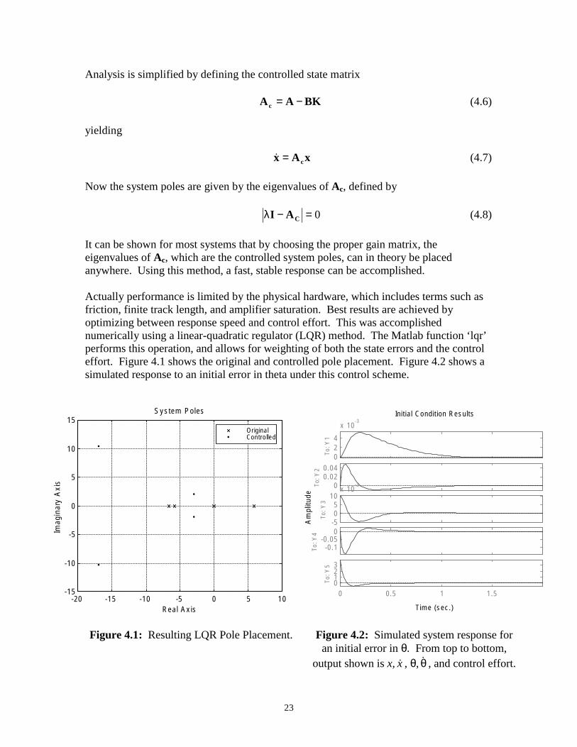
Actually performance is limited by the physical hardware, which includes terms such as friction, finite track length, and amplifier saturation. Best results are achieved by optimizing between response speed and control effort. This was accomplished numerically using a linear-quadratic regulator (LQR) method. The Matlab function ‘lqr’ performs this operation, and allows for weighting of both the state errors and the control effort. Figure 4.1 shows the original and controlled pole placement. Figure 4.2 shows a simulated response to an initial error in theta under this control scheme.

System Poles Initial Condition Results

l lled

OriginaContro

-3x 10

-3x 10

4 2

To: Y

1

0

0.04 0.02

Am

plitu

de

To: Y

4 To

: Y2

0 10 5

To: Y

3

0 -5 0

-0.05 -0.1

3 2 1 0To

: Y5

-15 0 0.5 1 1.5 -20 -15 -10 -5 0 5 10

Real Axis Time (sec.)

Figure 4.1: Resulting LQR Pole Placement. Figure 4.2: Simulated system response for an initial error in θ . From top to bottom,

output shown is x, x& , θ , θ & , and control effort.

23

-10

4.2 Standup Routine

The pendulum begins at rest, hanging downward in a stable equilibrium. The standup routine raises the pendulum to the inverted position, where the linear controller can stabilize it. It is important that the standup routine delivers the pendulum to the inverted position in a controlled, predictable fashion and at small angular velocity.

The basic strategy is to move the cart in such a motion that energy is gradually added to the pendulum. This first requires putting the cart under position control. Then a routine is needed to drive the cart’s position.

It is critical that this cart motion is synchronized with the pendulum swing. Precalculated movements and pauses will not suffice, being prone to system disturbances and uncertainty. Instead, a control method is needed which reacts to the current system state, and prescribes cart position accordingly.

4.2.1 Cart Position Control

The control of the cart position is straight forward, and will only be covered briefly. There exist many position control schemes alternate to what is presented here. However, it is required only that this controller act fast compared to pendulum movement and reject the disturbance forces caused by the pendulum swing. Significant overshoot is undesirable because it causes unpredictability.

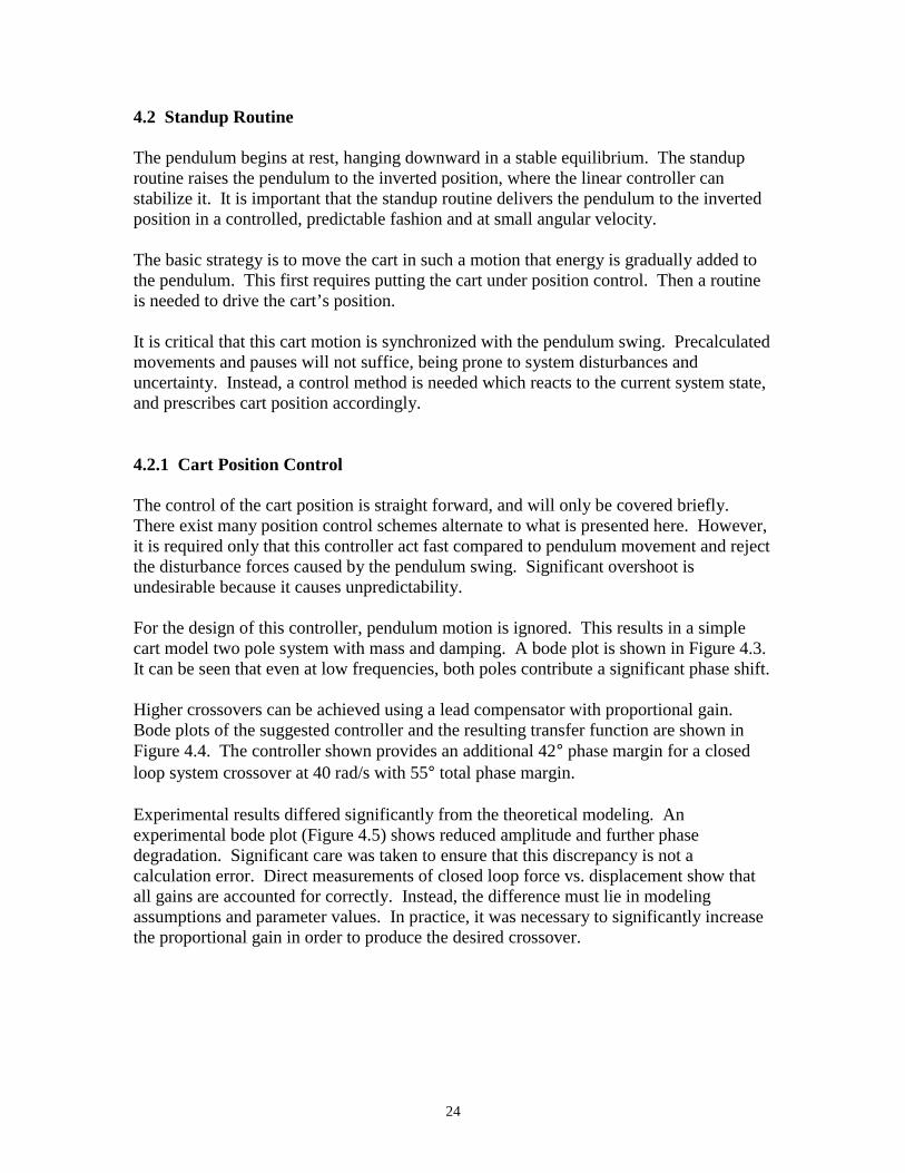
For the design of this controller, pendulum motion is ignored. This results in a simple cart model two pole system with mass and damping. A bode plot is shown in Figure 4.3. It can be seen that even at low frequencies, both poles contribute a significant phase shift.

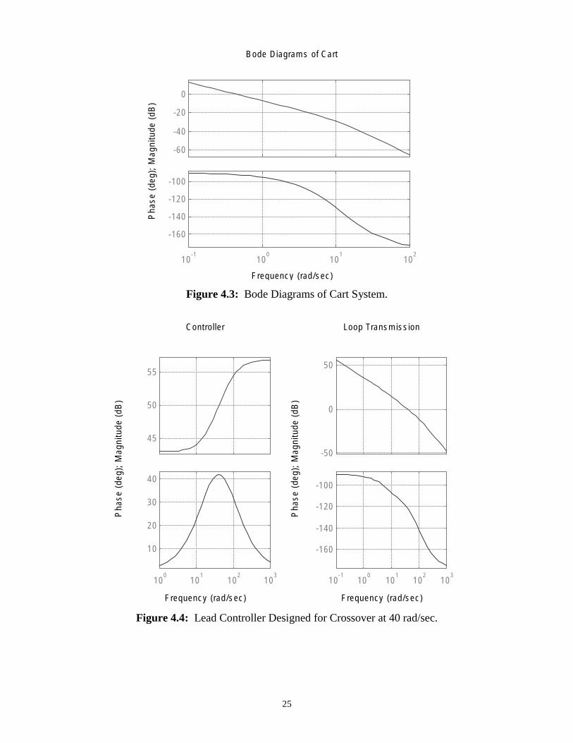
Higher crossovers can be achieved using a lead compensator with proportional gain. Bode plots of the suggested controller and the resulting transfer function are shown in Figure 4.4. The controller shown provides an additional 42° phase margin for a closed loop system crossover at 40 rad/s with 55° total phase margin.

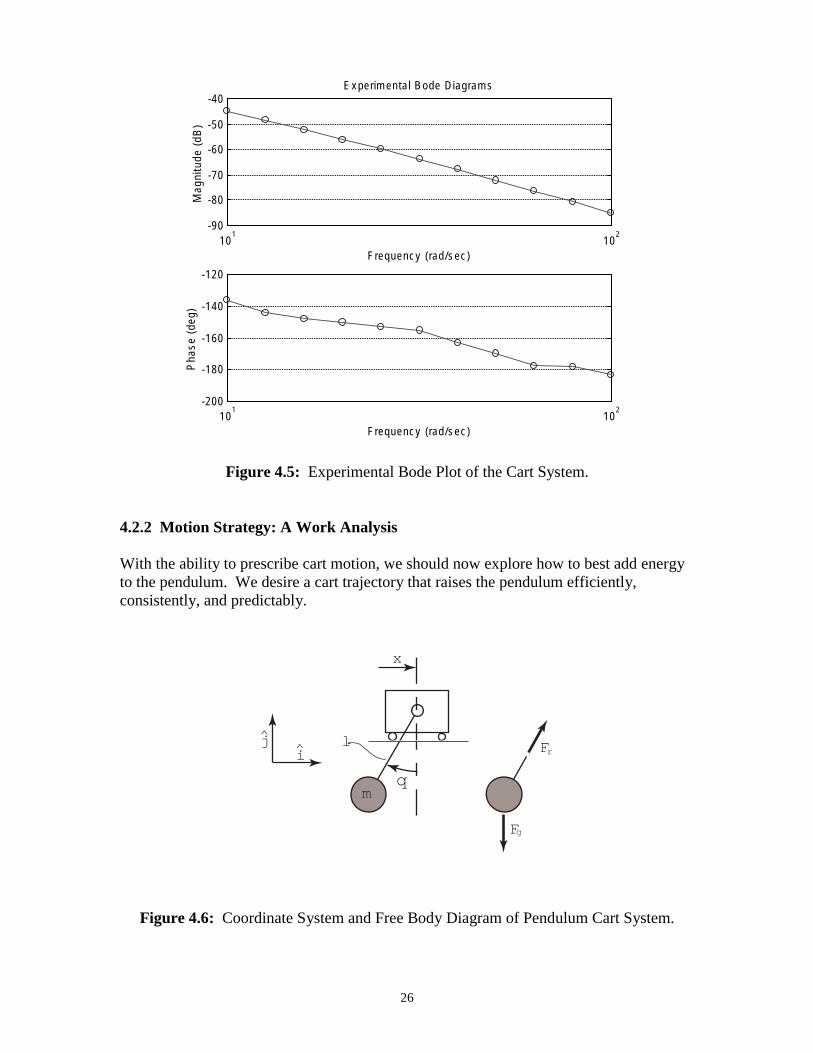
Experimental results differed significantly from the theoretical modeling. An experimental bode plot (Figure 4.5) shows reduced amplitude and further phase degradation. Significant care was taken to ensure that this discrepancy is not a calculation error. Direct measurements of closed loop force vs. displacement show that all gains are accounted for correctly. Instead, the difference must lie in modeling assumptions and parameter values. In practice, it was necessary to significantly increase the proportional gain in order to produce the desired crossover.

24

Bode Diagrams of Cart

i

0

Pha

se (

deg)

; M

agn

tude

(dB

) -60

-40

-20

-160

-140

-120

-100

-1 0 1 210 10 10 10

Frequency (rad/sec)

Figure 4.3: Bode Diagrams of Cart System.

Controller Loop Transmission

50 55

50

45

Pha

se (

deg)

; M

agni

tude

(dB

)

0

-50

40

20 -140

10 -160

-100

30 -120

0 1 2 3 -1 0 1 2 310 10 10 10 10 10 10 10 10

Frequency (rad/sec) Frequency (rad/sec)

Figure 4.4: Lead Controller Designed for Crossover at 40 rad/sec.

Pha

se (

deg)

; M

agni

tude

(dB

)

25

Experimental Bode Diagrams

i

-90

-80

-70

-60

-50

-40

Mag

ntu

de (

dB)

1 210 10

Frequency (rad/sec)

-200

-180

-160

-140

-120

Pha

se (

deg)

1 210 10

Frequency (rad/sec)

Figure 4.5: Experimental Bode Plot of the Cart System.

4.2.2 Motion Strategy: A Work Analysis

With the ability to prescribe cart motion, we should now explore how to best add energy to the pendulum. We desire a cart trajectory that raises the pendulum efficiently, consistently, and predictably.

q

x

Fr

m

Fg

ij l

Figure 4.6: Coordinate System and Free Body Diagram of Pendulum Cart System.

26

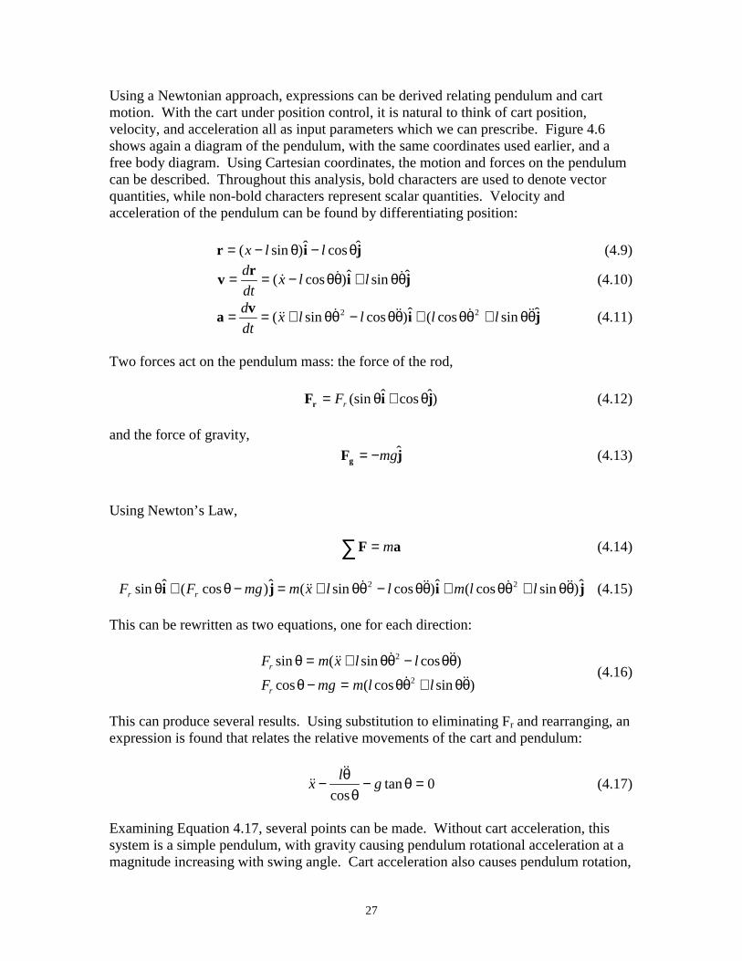
Using a Newtonian approach, expressions can be derived relating pendulum and cart motion. With the cart under position control, it is natural to think of cart position, velocity, and acceleration all as input parameters which we can prescribe. Figure 4.6 shows again a diagram of the pendulum, with the same coordinates used earlier, and a free body diagram. Using Cartesian coordinates, the motion and forces on the pendulum can be described. Throughout this analysis, bold characters are used to denote vector quantities, while non-bold characters represent scalar quantities. Velocity and acceleration of the pendulum can be found by differentiating position:

r = (x − l sin θ )i − l cos θ j (4.9)

v = dr = (x& − l cos θθ & )i + l sin θθ & j (4.10)dt

&& + l sin θθ & − l cos θθ )i + cos ( θθ & + l sin θθ j (4.11)a = dv = (x 2 && l 2 && ˆ dt

Two forces act on the pendulum mass: the force of the rod,

F = F (sin θ i + cos θ j) (4.12)r r

and the force of gravity,

F = − mgj (4.13)g

Using Newton’s Law,

∑ F = ma (4.14)

2F sin θ i + (F cos − θ mg) j = x m && cos ( θθ & + l sin θθ ) j (4.15)( && + l sin θθ & − l cos θθ )i + l m 2 && r r

This can be rewritten as two equations, one for each direction:

& 2 && F sin θ = x m ( && + l sin θθ − l cos θθ )r (4.16)& 2 && cos ( θθ + l sin θθ )F cos − θ mg = l m r

This can produce several results. Using substitution to eliminating Fr and rearranging, an expression is found that relates the relative movements of the cart and pendulum:

&& lθ x&& − − g tan θ = 0 (4.17)

cos θ

Examining Equation 4.17, several points can be made. Without cart acceleration, this system is a simple pendulum, with gravity causing pendulum rotational acceleration at a magnitude increasing with swing angle. Cart acceleration also causes pendulum rotation,

27

in addition to the effects of gravity. It can be seen that the direction of pendulum rotational acceleration depends on the direction of cart acceleration and whether the pendulum angle is above or below 90° . The effect of a cart acceleration on pendulum rotation is greatest when θ =0° (pendulum down) and at θ =180° (pendulum up).

Alternatively, Equation 4.16 can be solved for Fr, by eliminating && θ :

2&F = m(sin θ x&& + lθ + g cos θ ) (4.18)r

It is desirable to know how much work is done on the system when the cart is moved a small distance. This is simply the component of the force that is in the direction of movement, times the small displacement,

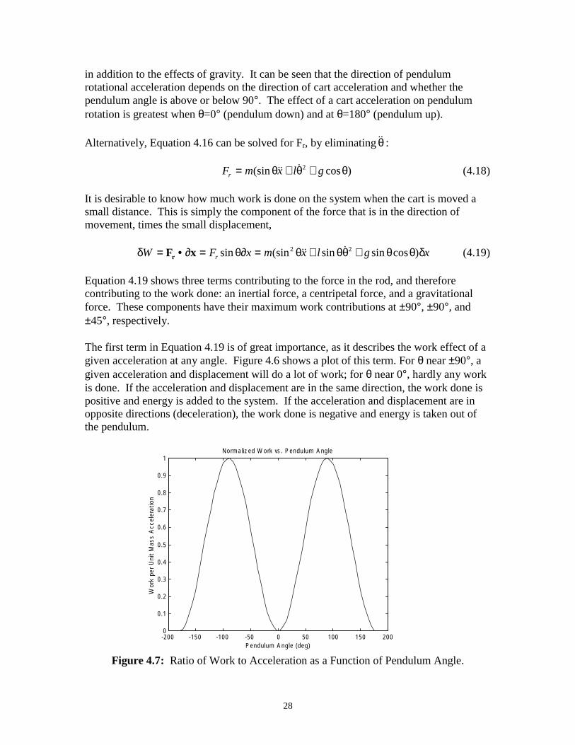
2 )δ W = F • ∂ x = F sin ∂θ x = m(sin θ x2 && + l sin θθ & + g sin θ cos δ θ x (4.19)r r

Equation 4.19 shows three terms contributing to the force in the rod, and therefore contributing to the work done: an inertial force, a centripetal force, and a gravitational force. These components have their maximum work contributions at ± 90° , ± 90° , and ± 45° , respectively.

The first term in Equation 4.19 is of great importance, as it describes the work effect of a given acceleration at any angle. Figure 4.6 shows a plot of this term. For θ near ± 90° , a given acceleration and displacement will do a lot of work; for θ near 0° , hardly any work is done. If the acceleration and displacement are in the same direction, the work done is positive and energy is added to the system. If the acceleration and displacement are in opposite directions (deceleration), the work done is negative and energy is taken out of the pendulum.

Normalized Work vs. Pendulum Angle

0

1

ile

rati

0.1

0.2

0.3

0.4

0.5

0.6

0.7

0.8

0.9

Wor

k pe

r U

nt

Mas

s A

cce

on

-200 -150 -100 -50 0 50 100 150 200 Pendulum Angle (deg)

Figure 4.7: Ratio of Work to Acceleration as a Function of Pendulum Angle.

28

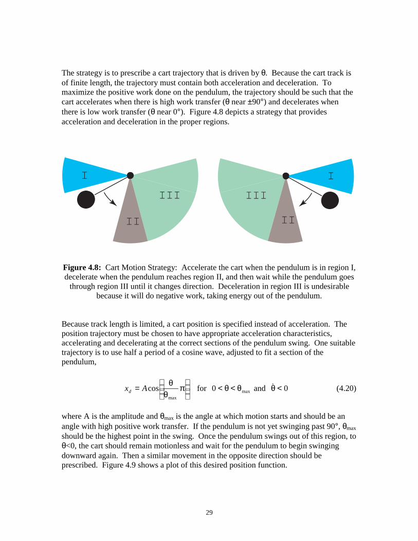
The strategy is to prescribe a cart trajectory that is driven by θ . Because the cart track is of finite length, the trajectory must contain both acceleration and deceleration. To maximize the positive work done on the pendulum, the trajectory should be such that the cart accelerates when there is high work transfer (θ near ± 90° ) and decelerates when there is low work transfer (θ near 0° ). Figure 4.8 depicts a strategy that provides acceleration and deceleration in the proper regions.

I

II

III

I

II

III

Figure 4.8: Cart Motion Strategy: Accelerate the cart when the pendulum is in region I, decelerate when the pendulum reaches region II, and then wait while the pendulum goes

through region III until it changes direction. Deceleration in region III is undesirable because it will do negative work, taking energy out of the pendulum.

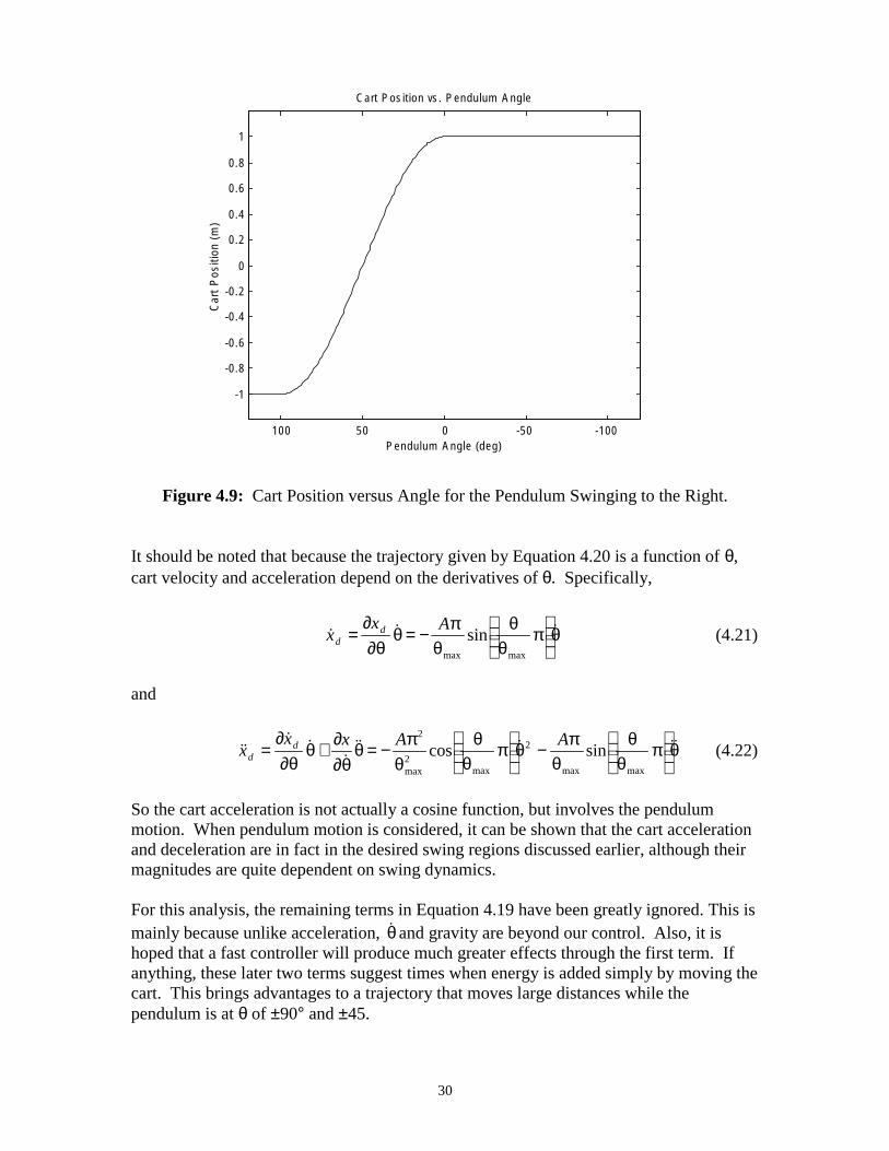
Because track length is limited, a cart position is specified instead of acceleration. The position trajectory must be chosen to have appropriate acceleration characteristics, accelerating and decelerating at the correct sections of the pendulum swing. One suitable trajectory is to use half a period of a cosine wave, adjusted to fit a section of the pendulum,

⎛ θ ⎞ xd = Acos⎜⎜ π⎟⎟ for 0 θ < θ < max and < θ & 0 (4.20)

⎝ θ max ⎠

where A is the amplitude and θ max is the angle at which motion starts and should be an angle with high positive work transfer. If the pendulum is not yet swinging past 90° , θ max

should be the highest point in the swing. Once the pendulum swings out of this region, to θ <0, the cart should remain motionless and wait for the pendulum to begin swinging downward again. Then a similar movement in the opposite direction should be prescribed. Figure 4.9 shows a plot of this desired position function.

29

Cart Position vs. Pendulum Angle

-1

0

1

-0.8

-0.6

-0.4

-0.2

0.2

0.4

0.6

0.8

Car

t P

ositi

on (

m)

100 50 0 -50 -100 Pendulum Angle (deg)

Figure 4.9: Cart Position versus Angle for the Pendulum Swinging to the Right.

It should be noted that because the trajectory given by Equation 4.20 is a function of θ , cart velocity and acceleration depend on the derivatives of θ . Specifically,

∂ xd &x& d = θ = − Aπ sin

⎛⎜⎜ θ π

⎞⎟⎟θ & (4.21)

θ∂ θ max ⎝ θ max ⎠

and

2 & ∂ x && Aπ Aπ

sin⎜⎜⎛ θ ⎞ && && d =

∂ x& d + θ &

θ = − cos ⎛⎜⎜ θ π

⎞⎟⎟θ & 2 − π⎟⎟θ (4.22)x

2θ∂ θ∂ θ max ⎝ θ max ⎠ θ max ⎝ θ max ⎠

So the cart acceleration is not actually a cosine function, but involves the pendulum motion. When pendulum motion is considered, it can be shown that the cart acceleration and deceleration are in fact in the desired swing regions discussed earlier, although their magnitudes are quite dependent on swing dynamics.

For this analysis, the remaining terms in Equation 4.19 have been greatly ignored. This is mainly because unlike acceleration, θ & and gravity are beyond our control. Also, it is hoped that a fast controller will produce much greater effects through the first term. If anything, these later two terms suggest times when energy is added simply by moving the cart. This brings advantages to a trajectory that moves large distances while the pendulum is at θ of ± 90° and ± 45.

30

In choosing this trajectory, it was critical that cart motion would allow the pendulum to move through the proper swing areas. Because both acceleration and deceleration is necessary for the finite length track, the pendulum must move from regions of high to low work transfer. For the trajectory described by equation 4.20, it is necessary that the pendulum indeed swings from ±θmax to 0°. Certain rapid cart movements will in fact cause the pendulum to accelerate upwards (see Equation 4.17), especially when the pendulum begins at a low height. In all considered trajectories, pendulum dynamics must be analyzed.

The pendulum motion can be analyzed using a Matlab numerical solver. Figure 4.10 shows the pendulum swing and cart movement with the pendulum beginning motionless at initial angles of 40°, 100°, and 160°. For small swings, the pendulum begins moving slowly, both because gravity has a smaller accelerating effect and because cart movement tends to push the pendulum in the opposite direction. Great acceleration at low starting angles would cause the pendulum to swing upwards. Matlab scripts are included in Appendix A.

While the trajectory described so far can efficiently add energy to the system, the standup routine requires additional algorithms at the start and finish. This trajectory is ineffective when the pendulum is at rest, because there is no work transfer when θ=0° and because of the pendulum dynamics discussed earlier. In this region, a quick change in cart position can be used to start the pendulum swinging. Several, well-timed jumps improve performance.

Pendulum Response Under Prescribed Cart Movement150

iti

0

50

100

0

50

100

iti

Pen

dulu

m A

ngle

(de

g) a

nd C

art

Pos

on (

mm

)

-100

-50

-100

-50

Pendulum AngleCart Pos on

150 150

100

50

0

-50

-100

0 0.2 0.4 0.6 0 0.2 0.4 0.6 0.2 0.4 0.6 0.8 Time (sec) Time (sec) Time (sec)

Figure 4.10: Pendulum and Cart Motion at Start Angles of 40°, 100°, and 160°. The cart moves only in a specific region of the swing in a trajectory that does work on the

pendulum. For smaller start angles, the pendulum motion begins very slowly.

31

As the pendulum approaches the inverted position, caution must be used that the pendulum reaches vertical at a low velocity. The trajectory described in equation 4.20 is still effective, but the amplitude must be reduced.

In summary, the standup routine should consist of the following subroutines, in this order:

1. Begin with a series of quick cart movements that begin the pendulum swinging.

2. Move the cart in a fashion that efficiently adds energy to the pendulum. 3. As the pendulum swings higher, gradually reduce cart movement amplitude so

that the pendulum approaches the inverted position in small increments and ultimately reaches vertical with small angular velocity.

Trajectory amplitude for subroutine 3 can be calculated as some function of the maximum height of the previous swing. This amplitude function can be tuned to produce the desired result of a gradual approach to vertical. More elaborate calculations could calculate the current energy of the pendulum, and prescribe a trajectory that delivered a certain amount of work. However, this calculation is computationally intensive, as it involves a work integral with continually changing parameters.

This algorithm is incapable of recovering if the pendulum is thrown over vertical with large velocity. It is therefore necessary to approach vertical carefully and gradually. Developing an algorithm that can recover opens the door to new strategies that are less cautious or perhaps intentionally throw the pendulum over the vertical, but this is beyond the scope of the present work.

32

5. Simulink Implementation

The routines and controllers described earlier, along with all general signal handling, are implemented using a single Simulink model. A Matlab script is used so that many system parameters are set from a single source. This section focuses on the details of the Simulink model, and assumes that the reader is somewhat familiar with general Simulink usage. First, we look at some useful Simulink methods. Then we give a complete explanation of the actual Simulink model. As the model contains numerous levels constructed with Simulink Subsystem blocks, analysis proceeds from the top down, beginning with the overall model before examining the Subsystems. In this fashion, the reader should learn the basic workings of the entire system before complicating matters with the internal details.

5.1 General Simulink Techniques

A few block combinations appear so frequently in the model that it is worth explaining them separately, before looking at the actual model. This will ease the explanation of later systems.

Methods of Switching Outputs

It is often desired to use different signals under different conditions. This is comparable to “if then else” statements and other logical operations in program scripts. Two methods of choosing outputs were found useful: enabled Subsystems and Multiport Switches.

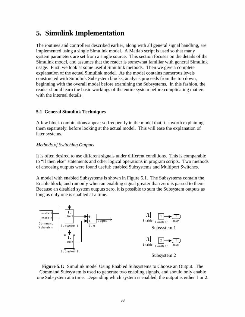
A model with enabled Subsystems is shown in Figure 5.1. The Subsystems contain the Enable block, and run only when an enabling signal greater than zero is passed to them. Because an disabled system outputs zero, it is possible to sum the Subsystem outputs as long as only one is enabled at a time.

enable 11 1enable 2

output

Sum

Out2

Out1

Subsystem 1

Enable Constant Out1 CommandSubsystem Subsystem 1

2 1 Enable Constant Out2

Subsystem 2

Subsystem 2

Figure 5.1: Simulink model Using Enabled Subsystems to Choose an Output. The Command Subsystem is used to generate two enabling signals, and should only enable

one Subsystem at a time. Depending which system is enabled, the output is either 1 or 2.

33

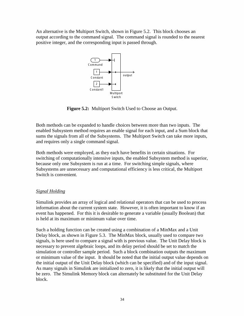
An alternative is the Multiport Switch, shown in Figure 5.2. This block chooses an output according to the command signal. The command signal is rounded to the nearest positive integer, and the corresponding input is passed through.

2

1

1

output

Constant1

Constant

Command

Multiport Switch

Figure 5.2: Multiport Switch Used to Choose an Output.

Both methods can be expanded to handle choices between more than two inputs. The enabled Subsystem method requires an enable signal for each input, and a Sum block that sums the signals from all of the Subsystems. The Multiport Switch can take more inputs, and requires only a single command signal.

Both methods were employed, as they each have benefits in certain situations. For switching of computationally intensive inputs, the enabled Subsystem method is superior, because only one Subsystem is run at a time. For switching simple signals, where Subsystems are unnecessary and computational efficiency is less critical, the Multiport Switch is convenient.

Signal Holding

Simulink provides an array of logical and relational operators that can be used to process information about the current system state. However, it is often important to know if an event has happened. For this it is desirable to generate a variable (usually Boolean) that is held at its maximum or minimum value over time.

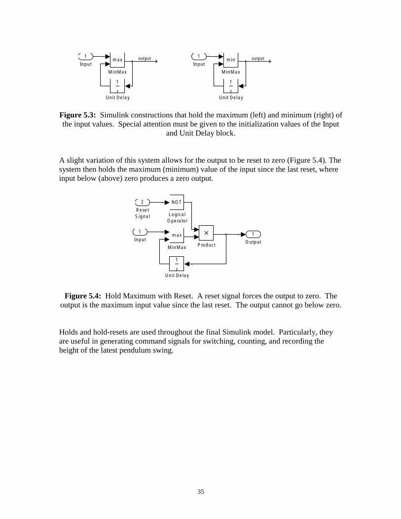
Such a holding function can be created using a combination of a MinMax and a Unit Delay block, as shown in Figure 5.3. The MinMax block, usually used to compare two signals, is here used to compare a signal with is previous value. The Unit Delay block is necessary to prevent algebraic loops, and its delay period should be set to match the simulation or controller sample period. Such a block combination outputs the maximum or minimum value of the input. It should be noted that the initial output value depends on the initial output of the Unit Delay block (which can be specified) and of the input signal. As many signals in Simulink are initialized to zero, it is likely that the initial output will be zero. The Simulink Memory block can alternately be substituted for the Unit Delay block.

34

1 1output max Input

MinMax

1

z z

1

min

MinMax

Input output

Unit Delay Unit Delay

Figure 5.3: Simulink constructions that hold the maximum (left) and minimum (right) of the input values. Special attention must be given to the initialization values of the Input

and Unit Delay block.

A slight variation of this system allows for the output to be reset to zero (Figure 5.4). The system then holds the maximum (minimum) value of the input since the last reset, where input below (above) zero produces a zero output.

1

z

1

l

2

1

Output Product

max

MinMax

NOT

LogicaOperator

Reset Signal

Input

Unit Delay

Figure 5.4: Hold Maximum with Reset. A reset signal forces the output to zero. The output is the maximum input value since the last reset. The output cannot go below zero.

Holds and hold-resets are used throughout the final Simulink model. Particularly, they are useful in generating command signals for switching, counting, and recording the height of the latest pendulum swing.

35

5.2 Overview of the Simulink Model

In this section, the entire Simulink model is outlined and explained. The model contains five levels of Subsystems. Analysis proceeds from the top level down. At each level, the function of all blocks and connections are described in moderate detail. Then the individual Subsystems are examined in the same manner.

Signals, blocks, and subsystems have been named to describe their function in the system. While this simplifies the model, it abstracts the original Simulink blocks. Specific Simulink blocks are best recognized in this report by their shape and appearance. Using the actual Simulink model file, blocks can be identified by their dialog boxes.

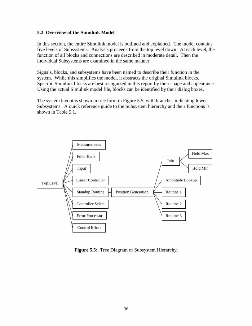
The system layout is shown in tree form in Figure 5.5, with branches indicating lower Subsystems. A quick reference guide to the Subsystem hierarchy and their functions is shown in Table 5.1.

Hold Max

Hold Min

Measurements

Filter Bank

Input

Linear Controller

Info

Top Level

Control Effort

Controller Select

Standup Routine

Error Processor

Position Generation Routine 1

Amplitude Lookup

Routine 3

Routine 2

Figure 5.5: Tree Diagram of Subsystem Hierarchy.

36

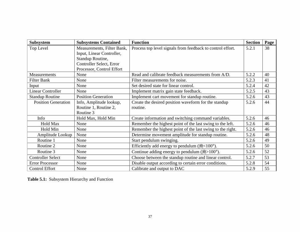
Subsystem Subsystems Contained Function Section Page Top Level Measurements, Filter Bank,

Input, Linear Controller, Standup Routine, Controller Select, Error Processor, Control Effort

Process top level signals from feedback to control effort. 5.2.1 38

Measurements None Read and calibrate feedback measurements from A/D. 5.2.2 40 Filter Bank None Filter measurements for noise. 5.2.3 41 Input None Set desired state for linear control. 5.2.4 42 Linear Controller None Implement matrix gain state feedback. 5.2.5 43 Standup Routine Position Generation Implement cart movement for standup routine. 5.2.6 43

Position Generation Info, Amplitude lookup, Routine 1, Routine 2, Routine 3

Create the desired position waveform for the standup routine.

5.2.6 44

Info Hold Max, Hold Min Create information and switching command variables. 5.2.6 46 Hold Max None Remember the highest point of the last swing to the left. 5.2.6 46 Hold Min None Remember the highest point of the last swing to the right. 5.2.6 46

Amplitude Lookup None Determine movement amplitude for standup routine. 5.2.6 48 Routine 1 None Start pendulum swinging. 5.2.6 49 Routine 2 None Efficiently add energy to pendulum (|θ|<100°). 5.2.6 50 Routine 3 None Continue adding energy to pendulum (|θ|>100°). 5.2.6 52

Controller Select None Choose between the standup routine and linear control. 5.2.7 53 Error Processor None Disable output according to certain error conditions. 5.2.8 54 Control Effort None Calibrate and output to DAC 5.2.9 55

Table 5.1: Subsystem Hierarchy and Function

37

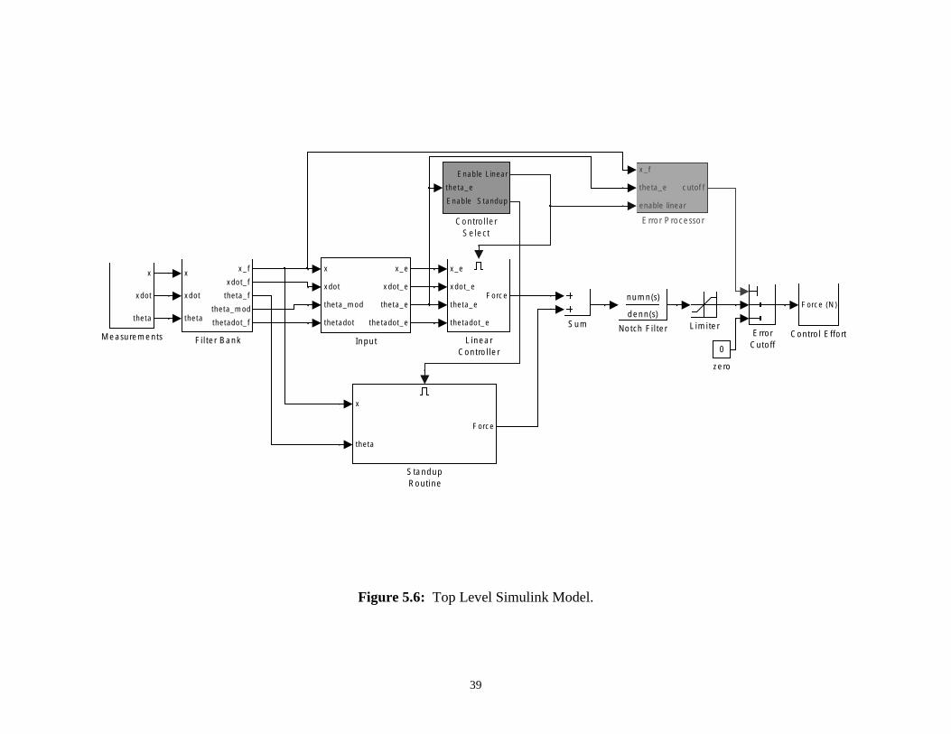
5.2.1 Top Level

The top level system is shown in Figure 5.6. Signals flow from left to right, with feedback signals entering in the Measurements block, traveling through various routines and controllers, and exiting to the hardware through the Control Effort block.

Feedback signals are interpreted in the Measurements Subsystem. This Subsystem includes the dSpace A/D conversion blocks and all necessary measurement calibrations. The resulting output from this block represents the physical quantities in SI units. Cart displacement x is represented in meters, cart velocity xdot is represented in meters per second, and pendulum angle theta is represented in radians. The directions of these measurements are consistent with that described in the theoretical derivation and apparatus summary earlier in this report.

These measurements are processed in the Filter Bank Subsystem. An array of low-pass filters is used for noise reduction. The angular velocity of the pendulum, thetadot, and a repeating angular position variable, theta_mod, are created in this block. All signals are labeled with the ‘_f’ extension to indicate that they have been filtered.

From here, the signals split. For linear control, the Input and Linear Controller Subsystems are used. For the standup routine, the Standup Routine Subsystem is used. Both generate an output signal representing the force, in Newtons, that should be applied to the cart. Signal switching is conducted using the method of enabled Subsystems, described in Section 5.1. The enable signal is generated by the Controller Select Subsystem, and the outputs are combined at the Sum block.

The Notch Filter is a Butterworth band stop filter for frequencies between 90 Hz and 120 Hz. This is necessary to eliminate a resonant mode involving deflection in the pendulum rod.

The Limiter block is used to protect the hardware. In this block, the requested force output is limited to 20 Newtons, limiting amplifier current to 4.6 amps.

The Error Processor Subsystem and Error Cutoff block form a safety system. The Error Cutoff block is simply a Multiport Switch, with zero as the second input. Under normal conditions, the Error Processor’s Subsystem outputs a value of 1, thereby selecting the Limiter block output, which is the force command signal. Under certain error conditions, the Error Processor will send a command cutoff signal of 2, which will select the zero input and thereby disable the output and stop the cart.

The Control Effort Subsystem calibrates the Force signal, and writes to the DAC. The analog signal from the DAC is used to drive the current amplifier.

38

0

x

il

x

l ler

i

x x

Fil

Sel

l

zero

Sum

theta

Force

numn(s)

denn(s)

Notch F ter

xdot

theta

Measurements

x_e

xdot_e

theta_e

thetadot_e

Force

Linear Contro

Lim ter

xdot

theta_mod

thetadot

x_e

xdot_e

theta_e

thetadot_e

Input

xdot

theta

x_f

xdot_f

theta_f

theta_mod

thetadot_f

ter Bank

x_f

theta_e

enable linear

cutof f

Error Processor

Error Cutoff

theta_e

Enable Linear

Enable Standup

Controller ect

Force (N)

Contro Effort

Standup Routine

Figure 5.6: Top Level Simulink Model.

39

5.2.2 Measurements

1

x

0

i

i

0

Di in

l

correct on

Term nator1

Sum1

Sum

-K-

PendPos

ther Ga

ENC_POS #1

ENC_POS #2

DS1102ENC_POS

ADC #1

ADC #2

ADC #3

ADC #4

DS1102ADC

.000

Constant1

3.7

CartVe

-K-

CartPos

3

theta

2

xdot

Terminator2

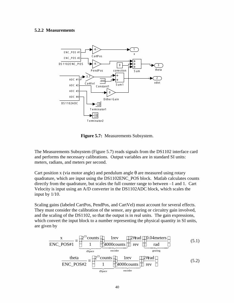
Figure 5.7: Measurements Subsystem.

The Measurements Subsystem (Figure 5.7) reads signals from the DS1102 interface card and performs the necessary calibrations. Output variables are in standard SI units: meters, radians, and meters per second.

Cart position x (via motor angle) and pendulum angle θ are measured using rotary quadrature, which are input using the DS1102ENC_POS block. Matlab calculates counts directly from the quadrature, but scales the full counter range to between –1 and 1. Cart Velocity is input using an A/D converter in the DS1102ADC block, which scales the input by 1/10.

Scaling gains (labeled CartPos, PendPos, and CartVel) must account for several effects. They must consider the calibration of the sensor, any gearing or circuitry gain involved, and the scaling of the DS1102, so that the output is in real units. The gain expressions, which convert the input block to a number representing the physical quantity in SI units, are given by

223⎛⎜⎜⎞⎟⎟

πrad 2

rev ⎟⎠

⎛⎜⎝⎠⎝ 4000counts4 3 443421 4 21 4

rev1 ⎛⎜⎝

⎞ ⎛⎜⎝

⎞⎟⎠

meters 04.0 ⎞countsx

ENC_POS#1 = ⎟

⎠rad421 443 4

(5.1)1

dSpace encoder gearing

⎛⎜⎜⎝

223 counts ⎞⎟⎟⎠

theta ⎛⎜⎝

rev1 ⎛⎜⎝

⎞⎟⎠

⎞⎟⎠

= πrad 2

rev (5.2)

ENC_POS#2 4000counts 43421 4 21 44 3 41

dSpace encoder

40

min 1 rad 2 πxdot ⎛10volts ⎛⎞ 1volt ⎛⎞ rpm 1000 ⎛⎜⎝

⎞ ⎛⎜⎝

⎞⎟⎠

⎛⎞⎟⎠

m/s 04.0 ⎞3volts1 4 43421 41 3 42 342

⎟⎠

⎜⎝

⎟⎠

⎜⎝

⎟⎠

⎜⎝ rad/s43 421

⎟⎠

⎜⎝

(5.3)=ADC#1 1 1volt 60s rev

dSpace circuit encoder gearing

A Dither Gain block was used in an earlier attempt to smooth the theta signal quantization. Ultimately, this gain was set to zero and the dither was not used. However, if desired, a dither signal could be brought in from ADC #2 on the DS1102.

All input values from the DS1102 are initialized to zero when the model is compiled. The state of the system at the time of compiling will therefore determine the zero value of all measurements. As designed, this model should be compiled with the cart stationary near the center of the track with the pendulum down and motionless.

5.2.3 Filter Bank

11

x x_f

1000

s+1000

2 200

s+200 xdot

Transfer Fcn4

2

xdot_f Transfer Fcn1

5

4

3

i

du/

i

i

3

thetadot_f

theta_mod

theta_f

200

s+200

Transfer Fcn3

1000

s+1000

Transfer Fcn2 mod

Math Funct on

dt

Derivat ve

2*p

Constant

theta

Figure 5.8: Filter Bank Subsystem.

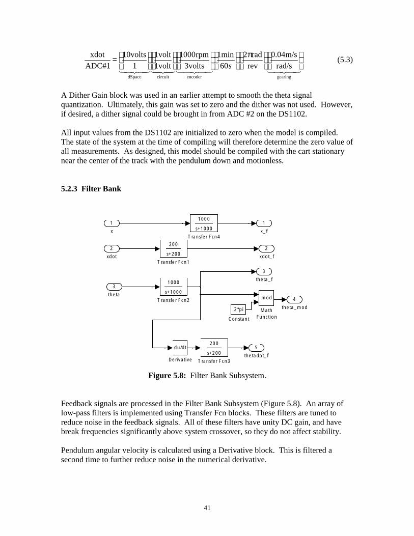
Feedback signals are processed in the Filter Bank Subsystem (Figure 5.8). An array of low-pass filters is implemented using Transfer Fcn blocks. These filters are tuned to reduce noise in the feedback signals. All of these filters have unity DC gain, and have break frequencies significantly above system crossover, so they do not affect stability.

Pendulum angular velocity is calculated using a Derivative block. This is filtered a second time to further reduce noise in the numerical derivative.

41

A repeating theta variable theta_mod is created using the mod function in a Math Function block. While the encoder measuring theta will measure multiple revolutions, the mod function subtracts these out, producing an output that is always between 0 and 2π. This variable is used for the linear controller, so that extra rotations do not produce an error. This is important because the pendulum can reach vertical in either the clockwise or counterclockwise direction.

5.2.3 Input

1 0

1 x_e x_d

Sum x

2 0

2 xdot_e

xdot_d Sum1

xdot

4

3

0

pi

4

3

thetadot_e

theta_e

thetadot_d

theta_d

Sum3

Sum2

thetadot

theta_mod

Figure 5.9: Input Subsystem.

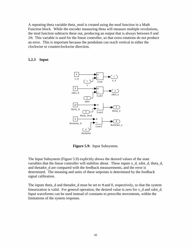
The Input Subsystem (Figure 5.9) explicitly shows the desired values of the state variables that the linear controller will stabilize about. These inputs x_d, xdot_d, theta_d, and thetadot_d are compared with the feedback measurements, and the error is determined. The meaning and units of these setpoints is determined by the feedback signal calibration.

The inputs theta_d and thetadot_d must be set to π and 0, respectively, so that the system linearization is valid. For general operation, the desired value is zero for x_d and xdot_d. Input waveforms can be used instead of constants to prescribe movements, within the limitations of the system response.

42

5.2.4 Linear Controller

1K

ix Gain

le

4

3

2

1

Force

Mux

Mux

Matr

Enab

theta_e

xdot_e

x_e

thetadot_e

Figure 5.10: Linear Controller Subsystem.

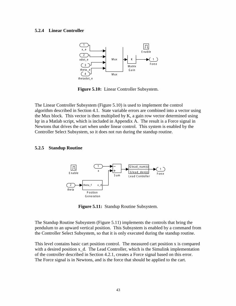
The Linear Controller Subsystem (Figure 5.10) is used to implement the control algorithm described in Section 4.1. State variable errors are combined into a vector using the Mux block. This vector is then multiplied by K, a gain row vector determined using lqr in a Matlab script, which is included in Appendix A. The result is a Force signal in Newtons that drives the cart when under linear control. This system is enabled by the Controller Select Subsystem, so it does not run during the standup routine.

5.2.5 Standup Routine

1 Gl

Gll l

le

2

1

x Force

Sum

theta_f x_d

ead_num(s)

ead_den(s) Lead Contro er

Enab

theta Position

Generation

Figure 5.11: Standup Routine Subsystem.

The Standup Routine Subsystem (Figure 5.11) implements the controls that bring the pendulum to an upward vertical position. This Subsystem is enabled by a command from the Controller Select Subsystem, so that it is only executed during the standup routine.

This level contains basic cart position control. The measured cart position x is compared with a desired position x_d. The Lead Controller, which is the Simulink implementation of the controller described in Section 4.2.1, creates a Force signal based on this error. The Force signal is in Newtons, and is the force that should be applied to the cart.

43

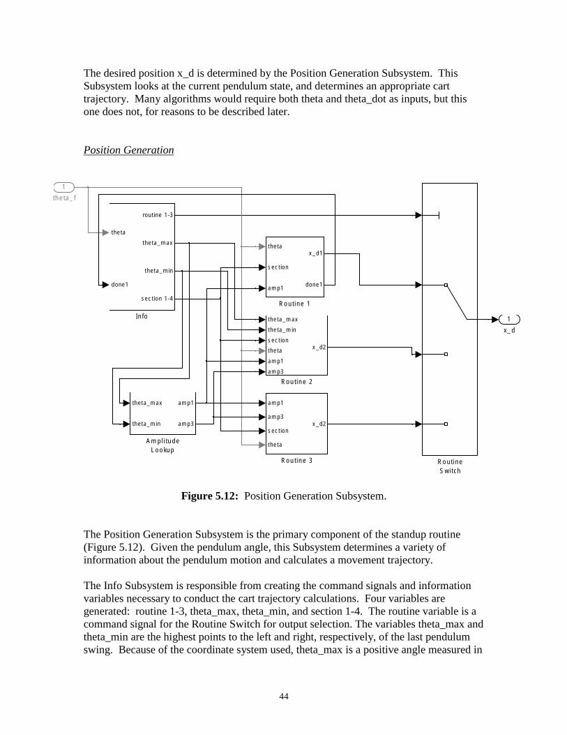
The desired position x_d is determined by the Position Generation Subsystem. This Subsystem looks at the current pendulum state, and determines an appropriate cart trajectory. Many algorithms would require both theta and theta_dot as inputs, but this one does not, for reasons to be described later.

Position Generation

1

i

in

i

i

i

i

i

in

i

in

1

x_d

amp1

amp3

sect on

theta

x_d2

theta_max

theta_m

sect on

theta

amp1

amp3

x_d2

Rout ne 2

theta

sect on

amp1

x_d1

done1

Rout ne 1

theta

done1

rout ne 1-3

theta_max

theta_m

sect on 1-4

Info

theta_max

theta_m

amp1

amp3

Amplitude Lookup

theta_f

Routine 3 Routine Switch

Figure 5.12: Position Generation Subsystem.

The Position Generation Subsystem is the primary component of the standup routine (Figure 5.12). Given the pendulum angle, this Subsystem determines a variety of information about the pendulum motion and calculates a movement trajectory.

The Info Subsystem is responsible from creating the command signals and information variables necessary to conduct the cart trajectory calculations. Four variables are generated: routine 1-3, theta_max, theta_min, and section 1-4. The routine variable is a command signal for the Routine Switch for output selection. The variables theta_max and theta_min are the highest points to the left and right, respectively, of the last pendulum swing. Because of the coordinate system used, theta_max is a positive angle measured in

44

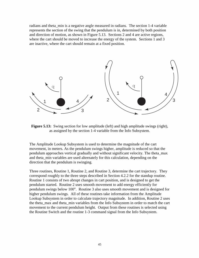
radians and theta_min is a negative angle measured in radians. The section 1-4 variable represents the section of the swing that the pendulum is in, determined by both position and direction of motion, as shown in Figure 5.13. Sections 2 and 4 are active regions, where the cart should be moved to increase the energy of the system. Sections 1 and 3 are inactive, where the cart should remain at a fixed position.

1

2 3 4

q

1

2 3

4

q

Figure 5.13: Swing section for low amplitude (left) and high amplitude swings (right), as assigned by the section 1-4 variable from the Info Subsystem.

The Amplitude Lookup Subsystem is used to determine the magnitude of the cart movement, in meters. As the pendulum swings higher, amplitude is reduced so that the pendulum approaches vertical gradually and without significant velocity. The theta_max and theta_min variables are used alternately for this calculation, depending on the direction that the pendulum is swinging.

Three routines, Routine 1, Routine 2, and Routine 3, determine the cart trajectory. They correspond roughly to the three steps described in Section 4.2.2 for the standup routine. Routine 1 consists of two abrupt changes in cart position, and is designed to get the pendulum started. Routine 2 uses smooth movement to add energy efficiently for pendulum swings below 100°. Routine 3 also uses smooth movement and is designed for higher pendulum swings. All of these routines take information from the Amplitude Lookup Subsystem in order to calculate trajectory magnitude. In addition, Routine 2 uses the theta_max and theta_min variables from the Info Subsystem in order to match the cart movement to the current pendulum height. Output from these routines is selected using the Routine Switch and the routine 1-3 command signal from the Info Subsystem.

45

1

Info

3

in

2

OR

or

- i/

l

>

>

<

<

le

<

l

hol

i/

<

>=

ge

>

g

1

c4

1

c2

0

c1

0

c

z

1

Sum

in

Hol in

Hol

2

Gain

i/

i /

2

theta_m

theta_max

100*p 180

ow angle

le3

le2

le1

max

d max2

100*p 180

high angle

ge1

AND

and1

AND

and

Unit Delay1

theta t_m

d M

theta t_max

d Max

100*p 180

100 deg

-100*p 180

done1

theta

Sum1 -100 deg1

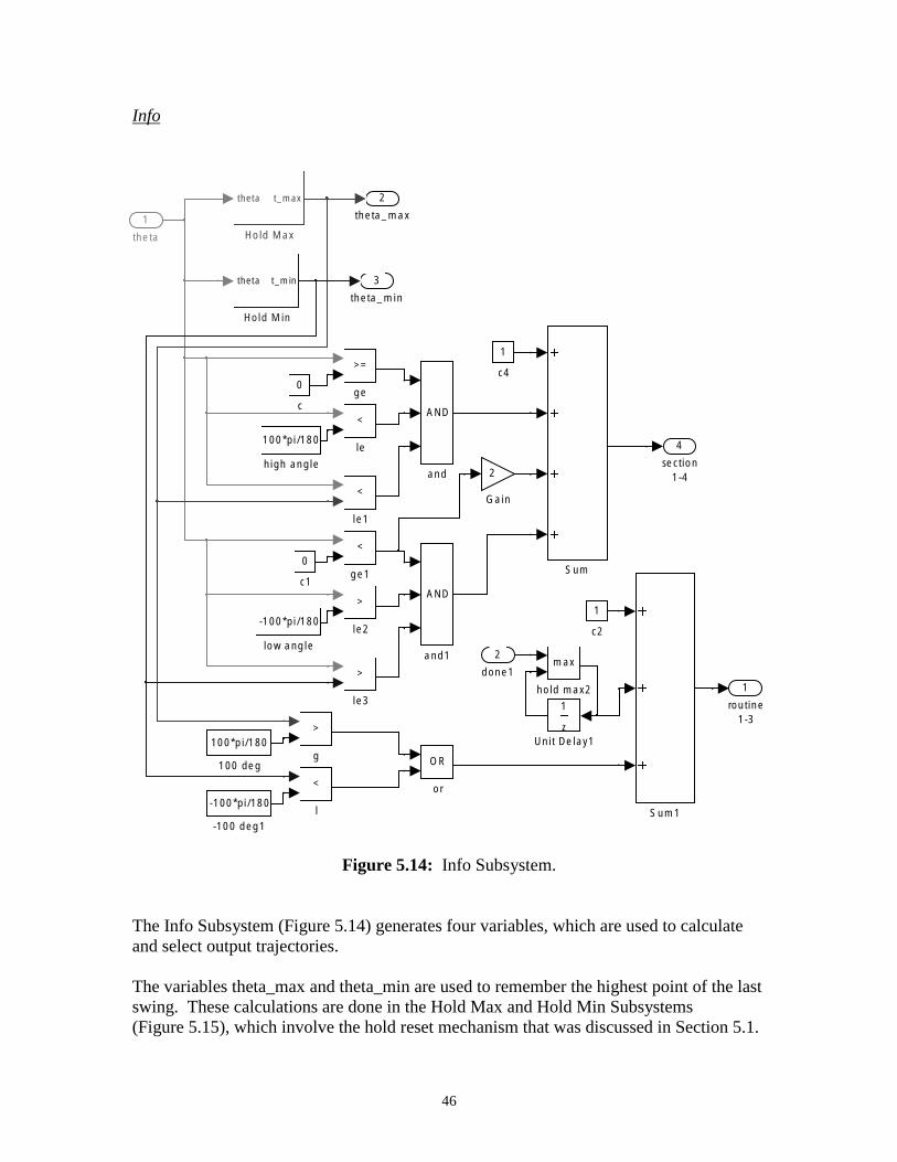
Figure 5.14: Info Subsystem.

The Info Subsystem (Figure 5.14) generates four variables, which are used to calculate and select output trajectories.

The variables theta_max and theta_min are used to remember the highest point of the last swing. These calculations are done in the Hold Max and Hold Min Subsystems (Figure 5.15), which involve the hold reset mechanism that was discussed in Section 5.1.

4

section 1-4

routine 1-3

46

1

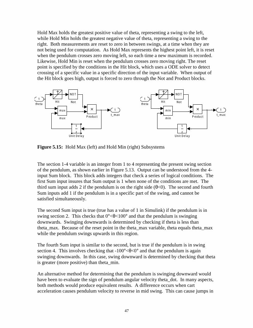
Hold Max holds the greatest positive value of theta, representing a swing to the left, while Hold Min holds the greatest negative value of theta, representing a swing to the right. Both measurements are reset to zero in between swings, at a time when they are not being used for computation. As Hold Max represents the highest point left, it is reset when the pendulum crosses zero moving left, so each time a new maximum is recorded. Likewise, Hold Min is reset when the pendulum crosses zero moving right. The reset point is specified by the conditions in the Hit block, which uses a ODE solver to detect crossing of a specific value in a specific direction of the input variable. When output of the Hit block goes high, output is forced to zero through the Not and Product blocks.

1

z

1

1

1

z

1

1

t_max max

max Product

NOT

Not Hit theta

t_max min

min Product

NOT

Not Hit theta

Unit Delay Unit Delay

Figure 5.15: Hold Max (left) and Hold Min (right) Subsystems

The section 1-4 variable is an integer from 1 to 4 representing the present swing section of the pendulum, as shown earlier in Figure 5.13. Output can be understood from the 4­input Sum block. This block adds integers that check a series of logical conditions. The first Sum input insures that Sum output is 1 when none of the conditions are met. The third sum input adds 2 if the pendulum is on the right side (θ<0). The second and fourth Sum inputs add 1 if the pendulum is in a specific part of the swing, and cannot be satisfied simultaneously.

The second Sum input is true (true has a value of 1 in Simulink) if the pendulum is in swing section 2. This checks that 0°<θ<100° and that the pendulum is swinging downwards. Swinging downwards is determined by checking if theta is less than theta_max. Because of the reset point in the theta_max variable, theta equals theta_max while the pendulum swings upwards in this region.

The fourth Sum input is similar to the second, but is true if the pendulum is in swing section 4. This involves checking that -100°<θ<0° and that the pendulum is again swinging downwards. In this case, swing downward is determined by checking that theta is greater (more positive) than theta_min.

An alternative method for determining that the pendulum is swinging downward would have been to evaluate the sign of pendulum angular velocity theta_dot. In many aspects, both methods would produce equivalent results. A difference occurs when cart acceleration causes pendulum velocity to reverse in mid swing. This can cause jumps in

47

the section 1-4 variable, leading to discontinuities in the desired position command. The method chosen is more tolerant, but still affected. Moreover, it is important to use cart trajectories that do not reverse the pendulum movement.

The routine 1-3 variable is also determined by summing logical signals. The first input to Sum1 begins output at 1. The second input holds the maximum value of done1, a variable generated inside the Routine 1 Subsystem that indicates that Routine 1 is finished. The third input checks that the pendulum is swing above 100°. But checking both theta_max and theta_min, the periodic resets of these variables do not cause routine 1-3 to drop back to a value of 2. However, the routine 1-3 variable can drop from 3 to 2 if the swing amplitude is for some reason reduced below 100°, perhaps through a disturbance.

Amplitude Lookup

1-1

Gain

2

in amp1 Look-Up

theta_m

Table1

1 2

theta_max amp3 Look-Up Table2

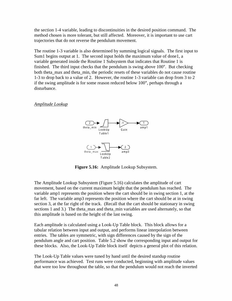
Figure 5.16: Amplitude Lookup Subsystem.

The Amplitude Lookup Subsystem (Figure 5.16) calculates the amplitude of cart movement, based on the current maximum height that the pendulum has reached. The variable amp1 represents the position where the cart should be in swing section 1, at the far left. The variable amp3 represents the position where the cart should be at in swing section 3, at the far right of the track. (Recall that the cart should be stationary in swing sections 1 and 3.) The theta_max and theta_min variables are used alternately, so that this amplitude is based on the height of the last swing.

Each amplitude is calculated using a Look-Up Table block. This block allows for a tabular relation between input and output, and performs linear interpolation between entries. The tables are symmetric, with sign differences caused by the sign of the pendulum angle and cart position. Table 5.2 show the corresponding input and output for these blocks. Also, the Look-Up Table block itself depicts a general plot of this relation.

The Look-Up Table values were tuned by hand until the desired standup routine performance was achieved. Test runs were conducted, beginning with amplitude values that were too low throughout the table, so that the pendulum would not reach the inverted

48

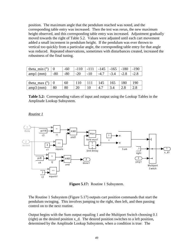
position. The maximum angle that the pendulum reached was noted, and the corresponding table entry was increased. Then the test was rerun, the new maximum height observed, and this corresponding table entry was increased. Adjustment gradually moved towards the right of Table 5.2. Values were adjusted until each cart movement added a small increment in pendulum height. If the pendulum was ever thrown to vertical too quickly from a particular angle, the corresponding table entry for that angle was reduced. Repeated observations, sometimes with disturbances created, increased the robustness of the final tuning.

theta_min (°) 0 -60 -110 -111 -145 -165 -180 -190 amp1 (mm) -80 -80 -20 -10 -4.7 -3.4 -2.8 -2.8

theta_max (°) 0 60 110 111 145 165 180 190 amp3 (mm) 80 80 20 10 4.7 3.4 2.8 2.8

Table 5.2: Corresponding values of input and output using the Lookup Tables in the Amplitude Lookup Subsystem.

Routine 1

>

l2

<

l1

==

==

ls

pi/8

c4

-pi/

c3

2

4

c1

2

i

1

equa

18 AND

and1

AND

and

sect on

theta

d max1

Unit Del

2

done1

.1

1

c

Sum

3

x_d1 right ay

amp1

Multiport Switch

ho

max

l

1

z

c2 equals1

Figure 5.17: Routine 1 Subsystem.

The Routine 1 Subsystem (Figure 5.17) outputs cart position commands that start the pendulum swinging. This involves jumping to the right, then left, and then passing control on to the next routine.

Output begins with the Sum output equaling 1 and the Multiport Switch choosing 0.1 (right) as the desired position x_d. The desired position switches to a left position, determined by the Amplitude Lookup Subsystem, when a condition is true: The

49

1

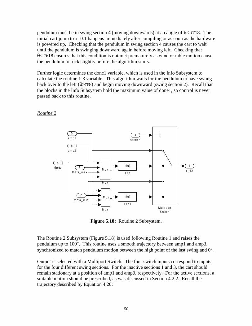
pendulum must be in swing section 4 (moving downwards) at an angle of θ<-π/18. The initial cart jump to x=0.1 happens immediately after compiling or as soon as the hardware is powered up. Checking that the pendulum in swing section 4 causes the cart to wait until the pendulum is swinging downward again before moving left. Checking that θ<-π/18 ensures that this condition is not met prematurely as wind or table motion cause the pendulum to rock slightly before the algorithm starts.

Further logic determines the done1 variable, which is used in the Info Subsystem to calculate the routine 1-3 variable. This algorithm waits for the pendulum to have swung back over to the left (θ>π/8) and begin moving downward (swing section 2). Recall that the blocks in the Info Subsystem hold the maximum value of done1, so control is never passed back to this routine.

Routine 2

1

Fcn

6

5

4

3

i

2

in

1 x_d2

Mux

Mux

Mux

Multiport

f(u)

Fcn1

f(u)

amp3

amp1

theta

sect on

theta_m

theta_max

Mux1 Switch

Figure 5.18: Routine 2 Subsystem.

The Routine 2 Subsystem (Figure 5.18) is used following Routine 1 and raises the pendulum up to 100°. This routine uses a smooth trajectory between amp1 and amp3, synchronized to match pendulum motion between the high point of the last swing and 0°.

Output is selected with a Multiport Switch. The four switch inputs correspond to inputs for the four different swing sections. For the inactive sections 1 and 3, the cart should remain stationary at a position of amp1 and amp3, respectively. For the active sections, a suitable motion should be prescribed, as was discussed in Section 4.2.2. Recall the trajectory described by Equation 4.20:

50

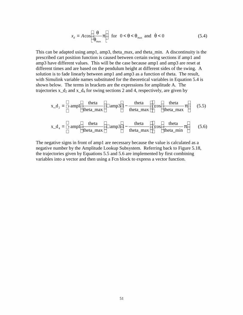
⎞⎟⎟⎠ πθ

θ ⎛⎜⎜⎝

for 0 θ<θ< max and θ& <0 (5.4)xd =Acos max

This can be adapted using amp1, amp3, theta_max, and theta_min. A discontinuity is the prescribed cart position function is caused between certain swing sections if amp1 and amp3 have different values. This will be the case because amp1 and amp3 are reset at different times and are based on the pendulum height at different sides of the swing. A solution is to fade linearly between amp1 and amp3 as a function of theta. The result, with Simulink variable names substituted for the theoretical variables in Equation 5.4 is shown below. The terms in brackets are the expressions for amplitude A. The trajectories x_d2 and x_d4 for swing sections 2 and 4, respectively, are given by

⎧ ⎫ ⎛ theta1amp-

theta_max

⎛ ⎜⎜⎝

⎞1amp3 −

⎛ ⎜⎜⎝

⎞ ⎞theta theta πx_d2 (5.5)+⎨⎩

⎧

⎜⎜⎝ ⎬⎭

cos theta_max

= ⎟⎟⎠ ⎟⎟⎠ ⎟⎟⎠theta_max

⎫ ⎛1amp-

theta_max

⎛ ⎜⎜⎝

⎞−

⎛ ⎜⎜⎝ 1amp3

⎞ ⎞theta theta theta πx_d4 (5.6)+⎨⎩

⎜⎜⎝ ⎬⎭

cos= ⎟⎟⎠ ⎟⎟⎠ ⎟⎟⎠theta_max theta_min

The negative signs in front of amp1 are necessary because the value is calculated as a negative number by the Amplitude Lookup Subsystem. Referring back to Figure 5.18, the trajectories given by Equations 5.5 and 5.6 are implemented by first combining variables into a vector and then using a Fcn block to express a vector function.

51

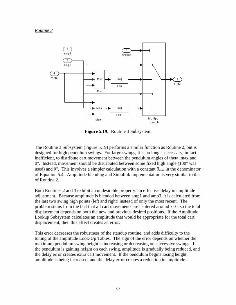
Routine 3

1

Swi

Fcn

4

3

i

2

1

x_d2

Mux

Mux1

Mux

Mux

Multiport tch

f(u)

Fcn1

f(u) theta

sect on

amp3

amp1

Figure 5.19: Routine 3 Subsystem.

The Routine 3 Subsystem (Figure 5.19) performs a similar function as Routine 2, but is designed for high pendulum swings. For large swings, it is no longer necessary, in fact inefficient, to distribute cart movement between the pendulum angles of theta_max and 0°. Instead, movement should be distributed between some fixed high angle (100° was used) and 0°. This involves a simpler calculation with a constant θmax in the denominator of Equation 5.4. Amplitude blending and Simulink implementation is very similar to that of Routine 2.

Both Routines 2 and 3 exhibit an undesirable property: an effective delay in amplitude adjustment. Because amplitude is blended between amp1 and amp3, it is calculated from the last two swing high points (left and right) instead of only the most recent. The problem stems from the fact that all cart movements are centered around x=0, so the total displacement depends on both the new and previous desired positions. If the Amplitude Lookup Subsystem calculates an amplitude that would be appropriate for the total cart displacement, then this effect creates an error.

This error decreases the robustness of the standup routine, and adds difficulty to the tuning of the amplitude Look-Up Tables. The sign of the error depends on whether the maximum pendulum swing height is increasing or decreasing on successive swings. If the pendulum is gaining height on each swing, amplitude is gradually being reduced, and the delay error creates extra cart movement. If the pendulum begins losing height, amplitude is being increased, and the delay error creates a reduction in amplitude.

52

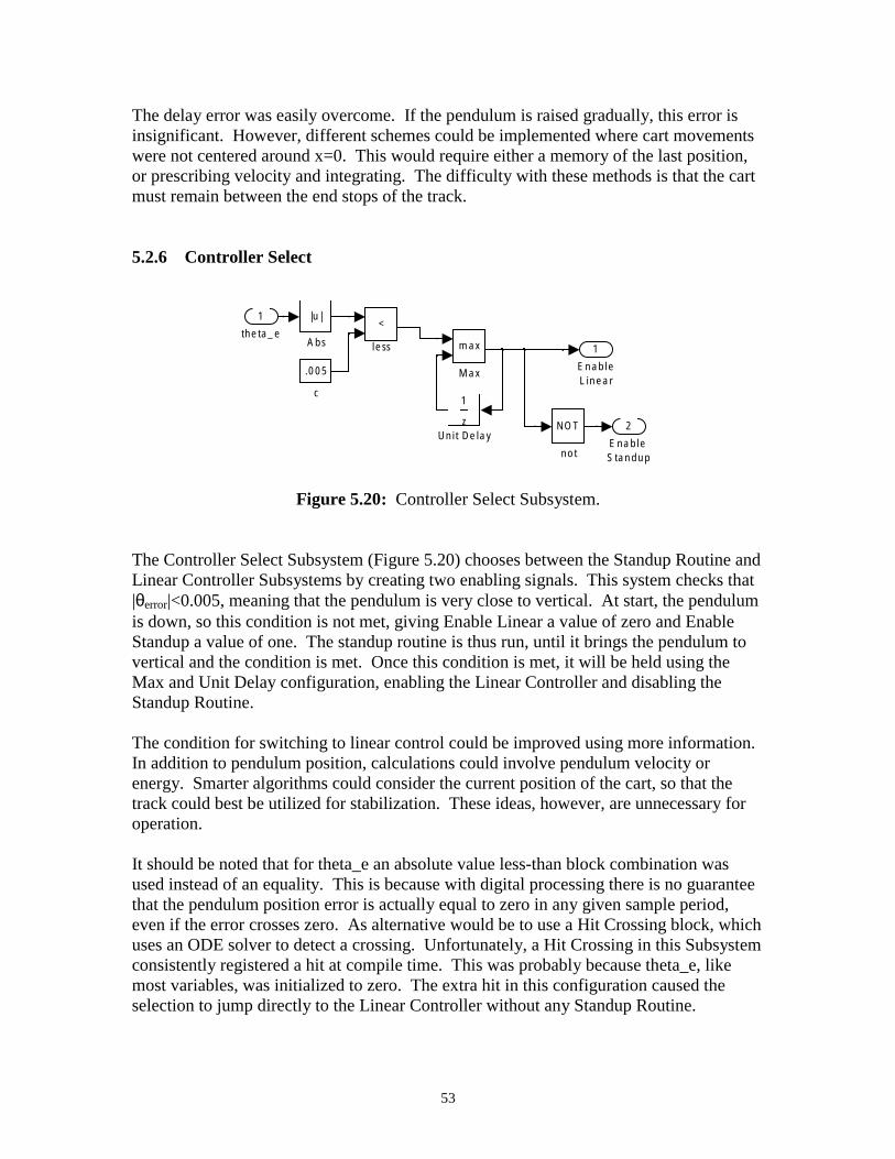
The delay error was easily overcome. If the pendulum is raised gradually, this error is insignificant. However, different schemes could be implemented where cart movements were not centered around x=0. This would require either a memory of the last position, or prescribing velocity and integrating. The difficulty with these methods is that the cart must remain between the end stops of the track.

5.2.6 Controller Select

2

l

1

le

c

z

1

Uni l

|u|

Abs

<1

less

Enab

EnabLinear

NOT

.005

t De ay

max

Max

theta_e

e not Standup

Figure 5.20: Controller Select Subsystem.

The Controller Select Subsystem (Figure 5.20) chooses between the Standup Routine and Linear Controller Subsystems by creating two enabling signals. This system checks that |θerror|<0.005, meaning that the pendulum is very close to vertical. At start, the pendulum is down, so this condition is not met, giving Enable Linear a value of zero and Enable Standup a value of one. The standup routine is thus run, until it brings the pendulum to vertical and the condition is met. Once this condition is met, it will be held using the Max and Unit Delay configuration, enabling the Linear Controller and disabling the Standup Routine.

The condition for switching to linear control could be improved using more information. In addition to pendulum position, calculations could involve pendulum velocity or energy. Smarter algorithms could consider the current position of the cart, so that the track could best be utilized for stabilization. These ideas, however, are unnecessary for operation.

It should be noted that for theta_e an absolute value less-than block combination was used instead of an equality. This is because with digital processing there is no guarantee that the pendulum position error is actually equal to zero in any given sample period, even if the error crosses zero. As alternative would be to use a Hit Crossing block, which uses an ODE solver to detect a crossing. Unfortunately, a Hit Crossing in this Subsystem consistently registered a hit at compile time. This was probably because theta_e, like most variables, was initialized to zero. The extra hit in this configuration caused the selection to jump directly to the Linear Controller without any Standup Routine.

53

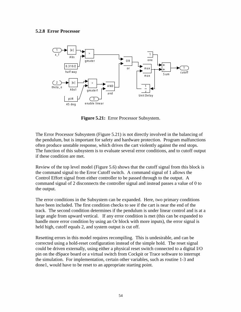
5.2.8 Error Processor

OR

or hal

>

>

|u|

|u|

Abs

pi/4 3

2

1

0.310/2

f way

greater1

greater

AND

and Abs1

theta_e

x_f

1

1

z

1

cutoff

one

max

max Sum

Unit Delay

45 deg enable l inear

Figure 5.21: Error Processor Subsystem.

The Error Processor Subsystem (Figure 5.21) is not directly involved in the balancing of the pendulum, but is important for safety and hardware protection. Program malfunctions often produce unstable response, which drives the cart violently against the end stops. The function of this subsystem is to evaluate several error conditions, and to cutoff output if these condition are met.

Review of the top level model (Figure 5.6) shows that the cutoff signal from this block is the command signal to the Error Cutoff switch. A command signal of 1 allows the Control Effort signal from either controller to be passed through to the output. A command signal of 2 disconnects the controller signal and instead passes a value of 0 to the output.

The error conditions in the Subsystem can be expanded. Here, two primary conditions have been included. The first condition checks to see if the cart is near the end of the track. The second condition determines if the pendulum is under linear control and is at a large angle from upward vertical. If any error condition is met (this can be expanded to handle more error condition by using an Or block with more inputs), the error signal is held high, cutoff equals 2, and system output is cut off.

Resetting errors in this model requires recompiling. This is undesirable, and can be corrected using a hold-reset configuration instead of the simple hold. The reset signal could be driven externally, using either a physical reset switch connected to a digital I/O pin on the dSpace board or a virtual switch from Cockpit or Trace software to interrupt the simulation. For implementation, certain other variables, such as routine 1-3 and done1, would have to be reset to an appropriate starting point.

54

5.2.9 Control Effort

Gain

1 -K- DAC #1

DAC #2

DAC #3

DAC #4

DS1102DAC

Force (N)

Ground1

Figure 5.22: Control Effort Subsystem.

The Control Effort Subsystem calibrates and outputs the Control Effort to the DS1102. The input Force refers to the force, in Newtons, that should be delivered to the cart. For calibration, a gain is necessary which counteracts gains in the dSpace DAC write, current amplifier, and motor.

⎛⎜⎜⎛⎜⎜

⎞⎟⎟⎞⎟⎟

⎛ 1

⎝⎠⎝⎞⎟⎠ 2amps42 1 1 43

volt1 1K =

volts 10 ⎜⎝ 421 4 3

(5.7)⎠N/amp 25.4

42 4 4 3 4 dSpace amplifier motor

55

6. Recommendations

Although the current system is fully function, several improvements can be made. These are outlined here for the benefit of anyone continuing this project, and to increase the general understanding of the subject. Many of these recommendations are also covered in specific sections of this report.

When cart position control was designed for the standup routine (Section 4.2.1), a significant discrepancy between theoretical predictions and experimental results was discovered. This was attributed to unmodeled effects, and was overcome by adjusting gain to match the experimental response. However, design of the linear controller is based completely on theoretical behavior, and involves many of the parameters found to be in error for cart position control. While the linear controller is functional, it is suspected that improvements could be made if this discrepancy were resolved. It is therefore recommended that additional behavior, including dry friction, belt compliance, and motor and amplifier dynamics, be considered. Alternatively, some of these effects could be reduced or eliminated.

The physical hardware is unsuccessful at constraining the pendulum to planar motion. In fact, a mode of vibration exists in which the pendulum deflects in a direction parallel to its axis of rotation. This unfortunately couples with cart motion, despite their orthogonality. This causes a resonance at a frequency of about 9.5 Hz, producing significant jitter in linear control. This mode should be eliminated by replacing the pendulum joint and rod with a structure that is rigid in this direction.

The Simulink model could be improved in several ways, which were discussed at appropriate points in Section 5. A significant improvement would be to allow for resets of the model without recompile. The current model runs the routine only once per compile, and will shut off when errors occur. It would be desirable to have an external reset switch that would restart the routine.

A second modification of the Simulink model involves the cart motions in the standup routine. Currently, all motion is centered about x=0. This is undesirable because the total magnitude of each movement depends on the starting position. The solution is to prescribe cart movement magnitudes, instead of prescribing the next desired location. This can be accomplished either be prescribing velocity and integrating, or by calculating the new desired position relative to the previous one. Implementing such a scheme would improve standup routine reliability and allow for faster standups.

A final recommendation is to use a reduced-order observer for the determination of &pendulum angular velocity θ . Such an implementation would eliminate the numerical

derivative that is used in the current model. It must be noted that this observer can only be used for linear control, where the system can be modeled using a LTI system. Also, the observer must be initialized correctly at an appropriate time.

56

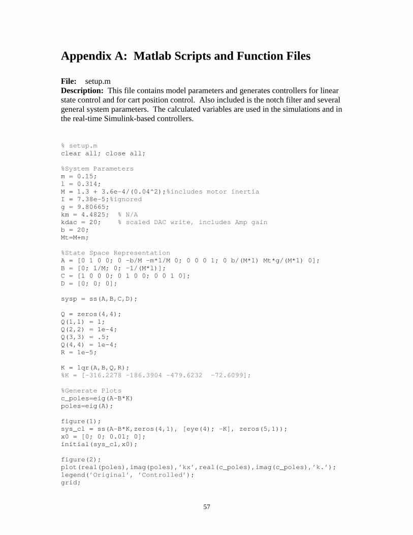
Appendix A: Matlab Scripts and Function Files

File: setup.m Description: This file contains model parameters and generates controllers for linear state control and for cart position control. Also included is the notch filter and several general system parameters. The calculated variables are used in the simulations and in the real-time Simulink-based controllers.

% setup.mclear all; close all;

%System Parametersm = 0.15;l = 0.314;M = 1.3 + 3.6e-4/(0.04^2);%includes motor inertiaI = 7.38e-5;%ignoredg = 9.80665; km = 4.4825; % N/A kdac = 20; % scaled DAC write, includes Amp gain b = 20; Mt=M+m;

%State Space RepresentationA = [0 1 0 0; 0 -b/M -m*l/M 0; 0 0 0 1; 0 b/(M*l) Mt*g/(M*l) 0];B = [0; 1/M; 0; -1/(M*l)];C = [1 0 0 0; 0 1 0 0; 0 0 1 0];D = [0; 0; 0];

sysp = ss(A,B,C,D);

Q = zeros(4,4);Q(1,1) = 1;Q(2,2) = 1e-4;Q(3,3) = .5;Q(4,4) = 1e-4;R = 1e-5;

K = lqr(A,B,Q,R);%K = [-316.2278 -186.3904 -479.6232 -72.6099];

%Generate Plotsc_poles=eig(A-B*K)poles=eig(A);

figure(1);sys_cl = ss(A-B*K,zeros(4,1), [eye(4); -K], zeros(5,1));x0 = [0; 0; 0.01; 0];initial(sys_cl,x0);

figure(2);plot(real(poles),imag(poles),’kx’,real(c_poles),imag(c_poles),’k.’);legend(’Original’, ’Controlled’);grid;

57

title(’System Poles’);xlabel(’Real Axis’);ylabel(’Imaginary Axis’);

% create a notch filter at the resonant frequency[numn,denn] = butter(3,2*pi*[90 120],’stop’,’s’);

%Controller (lead), label 2, Values for lag are included, but not used.Ka=2;Gsys=tf([0 0 1],[M+m b 0]);wc=40;wctr=wc;Kc=10*274.5909;a1=5;

t1=1/(wctr*sqrt(a1));t3=1/(wc/50);%laga3=10;Glead_num=Kc*[a1*t1 1];Glead_den=[t1 1];Glag_num=a3*[t3 1];Glag_den=[a3*t3 1];Gc_num=conv(Glead_num,Glag_num);Gc_den=conv(Glead_den,Glag_den);Glead=tf(Glead_num,Glead_den);Glag=tf(Glag_num,Glag_den);Gc2=Glead*Glag;L2=Glead*Glag*Ka*km*Gsys;

%For controller design[m p]=bode(L2,wc);1/m

%standup params (many were ultimately not used)c=0.07;theta_high=100*pi/180;sample_T=0.0005;sat=40/Kc;%not used

File: swing.m Descirption: Numerical simulation of cart and pendulum movements. Cart movement is defined by Equation 4.20 in this report. This script calls the function ‘ydot’, included, which defines the system differential equations.

%swing_rglobal A t_max;

t_max=100*pi/180;%Angle at which cart motion begins%motion ends at theta=0A=.06;%cart motion amplitudey0=[160*pi/180 0];%initial angle and velocity of pendulum

[t y]=ode45(’ydot’,[0 1],y0);%use ODE solver for theta and theta_dottheta=y(:,1);

58

theta_deg=theta*180/pi;

%calculate cart position x from thetan=size(t);x_d=zeros(n);for i=1:n

if and(theta(i)<t_max, theta(i)>0) x_d(i)=A*cos(theta(i)*pi/t_max);

else if theta(i)>t_max x_d(i)=-A;

elsex_d(i)=A;

end end

end

%plot x and theta vs. timeplot(t,theta_deg,’-’,t,1000*x_d,’--’);title(’Pendulum Response Under Prescribed Cart Movement’);xlabel(’Time (sec)’);ylabel(’Pendulum Angle (deg) and Cart Position (mm)’);legend(’Pendulum Angle’, ’Cart Position’)

File: ydot.m Description: Matlab function defining the system differential equation General dynamics were derived in Equation 4.17, where &&x is defined by 4.22. Because x is a function of θ, differential analysis involves only θ and θ& .

function dydt=ydot(t,y);

global A t_max;%use values set in the swing.m file

theta=y(1);theta_dot=y(2);

g=9.8;l=.314;

ddt_theta=theta_dot;

if and(theta<t_max, theta>0)%Cart moving, ddt_theta_dot involves cartacceleration

ddt_theta_dot=(-(A*pi^2/t_max^2)*cos(theta*pi/t_max)*theta_dot^2-g*tan(theta) )/( l/cos(theta)+(A*pi/t_max)*sin(theta*pi/t_max) );else%cart stationary, x_double_dot=0

ddt_theta_dot=-g*tan(theta)*cos(theta)/l;end

dydt(1)=ddt_theta;dydt(2)=ddt_theta_dot;dydt=dydt’;

59

Appendix B: Operating the Pendulum-Cart System

1. Check the Hardware

The system has several components, currently wired together but not physically inseparable. You should have (1) a large platform with pendulum-cart and motor, (2) a current amplifier, and (3) a small aluminum box housing a circuit and a DS1102 interface card. There are two switches; set them to OFF and DISABLE. Check that the amplifier is plugged in, and that the computer is connencted to the interface card. Be sure that the pendulum motion is unobstructed for all cart and pendulum positions.

2. Software

To operate the pendulum system, you need two files: the Simulink model pendem.mdl and a Matlab script setup.m. For simplicity, copy both files to a common directory, and run Matlab in that directory.

At the Matlab prompt: Type ‘setup’ to run setup.m. Type ‘pendem’ to open Simulink with the pendem.mdl Simulink model.

3. Building the Simulink model

Before you build, the hardware must be set accordingly: 1) Make sure the ‘Enable/Disable’ switch is set to DISABLE. 2) Set amplifier switch to ON (this affects velocity measurement initialization). 3) Center the Pendulum on the track, and stabilize with pendulum down.

Now build the model, using RTW Build in the Simulink Tools menu.

Wait until the model is built, then flip the ‘Enable/Disable’ switch to ENABLE to begin routine. Cart and pendulum motion will begin immediately.

4. Operation Notes:

If the system malfunctions, flip the ‘Enable/Disable’ switch to DISABLE. Make sure this switch is safely away from pendulum motion (before you compile).

The model also disables under certain error conditions, sending zero to output. If it disables, it is necessary to recompile the model. You can deliberately disable the model by using these error conditions: move the cart to the end of the track or cause a pendulum angle of more than 45° from vertical while the system is under linear control.

If the ‘Enable/Disable’ switch is set to ENABLE while compiling, Pendulum motion will begin when compiling is complete. However, while compiling, output is commanded by

60

the previous DSP application. This is fine only if this model was the previous application and an error condition was met. Otherwise, make sure the ‘Enable/Disable’ switch is set to DISABLE.

5. Cockpit Interface

A Cockpit file, called pendem.css, has been included. This file contains displays of the state variables and other basic model parameters. To use, run cockpit, then open pendem from the Cockpit File menu. After compiling the Simulink model, load the trace file pendem, using the Cockpit File menu. Click on the Start button to begin.

61

References

1. Franklin, Gene F., Powell, David J., and Emami-Maeini, Abbas, Feedback Control of Dynamic Systems, Addison-Wesley, New York, 1994.

2. Dorf, Richard C., Modern Control Systems, Addison-Wesley, New York, 1992.

3. Williams, James H. Jr., Fundamentals of Applied Dynamics, John Wiley & Sons, New York, 1996.

4. Friedland, Bernard, Control System Design, McGraw-Hill, Boston, 1986.

5. Rowell, Derek and Wormley, David N., System Dynamics: An Introduction, Prentice-Hall, Upper Saddle River, New Jersey, 1997.

6. Gould, L. A., Markey, W. R., Roberge, J. K., and Trumper, D. L., Control Systems Theory, 1997.

7. Spong, Mark, W., The Swing Up Control Problem for the Acrobot, IEEE Control Ststems, pp. 49-55, February 1995.

8. Using Simulink, The Mathworks, 1998.

62