Embed Size (px)
Citation preview
Standards
Certification
Education & Training
Publishing
Conferences & Exhibits
eBook available!
Table of Contents
View Excerpt
Buy the Book
Table of Contents
View Excerpt
Buy the Book
Control Systems Engineering Exam Reference Manual
A Practical Study GuideFourth Edition
For the NCEES ProfessionalEngineering (PE) Licensing Examination
Bryon Lewis, PE (CSE), CAP, CCST III
Controls engineering encompasses a broad range of industries: power, paper and pulp, pharmaceuticals, manufacturing, water treatment, and chemical plants. Although this fourth edition addresses many different applications used by all these industries, it focuses on petrochemical applications.
The National Council of Examiners for Engineering and Surveying (NCEES) Professional Engineer (PE)/Control Systems Engineer (CSE) exam tends to be concentrated toward chemical and pharmaceutical plant design applications of code and control systems. The purpose of this book is to introduce new engineers to the depth of knowledge they will need to tackle the NCEES PE/CSE exam.
v
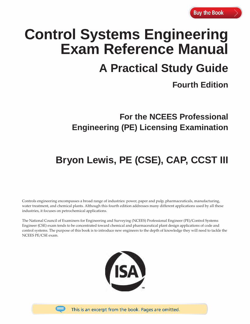
Contents
Introduction to This Study Guide . . . . . . . . . . . . . . . . . . . . . . . . . . . . . . . . . . . . .xv
Chapter 1 Welcome to Control Systems EngineeringLicensing as Professional Engineer/Control Systems Engineer . . . . . . . . 1Why Become a Professional Engineer? . . . . . . . . . . . . . . . . . . . . . . . . . . . . . 2This Is the Fourth Edition of This Study Manual . . . . . . . . . . . . . . . . . . . . 3Notes for Reading This Manual . . . . . . . . . . . . . . . . . . . . . . . . . . . . . . . . . . . 3Overview of Recommended Flowchart of Study for the CSE . . . . . . . . . . 5
Chapter 2 Exam General Information . . . . . . . . . . . . . . . . . . . . . . . . . . . . . . . . . .7State Licensing Requirements . . . . . . . . . . . . . . . . . . . . . . . . . . . . . . . . . . . . . 7Eligibility . . . . . . . . . . . . . . . . . . . . . . . . . . . . . . . . . . . . . . . . . . . . . . . . . . . . . . 7Exam Schedule . . . . . . . . . . . . . . . . . . . . . . . . . . . . . . . . . . . . . . . . . . . . . . . . . 8Description of Exam . . . . . . . . . . . . . . . . . . . . . . . . . . . . . . . . . . . . . . . . . . . . . 8Exam Content – The NCEES 2019 Specifications . . . . . . . . . . . . . . . . . . . . . 8
I. Measurement – 20 Questions . . . . . . . . . . . . . . . . . . . . . . . . . . . . . . . 9II. Control Systems – 20 Questions . . . . . . . . . . . . . . . . . . . . . . . . . . . . . 9III. Final Control Elements – 16 Questions . . . . . . . . . . . . . . . . . . . . . 11IV. Signals, Transmission, and Networking – 12 Questions . . . . . . . 12V. Safety Systems – 12 Questions . . . . . . . . . . . . . . . . . . . . . . . . . . . . . 13
Exam Scoring . . . . . . . . . . . . . . . . . . . . . . . . . . . . . . . . . . . . . . . . . . . . . . . . . 13
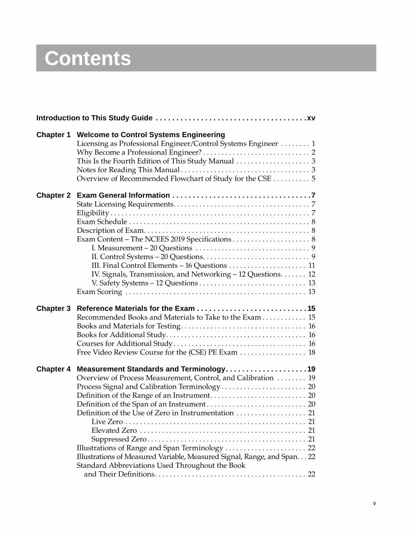
Chapter 3 Reference Materials for the Exam . . . . . . . . . . . . . . . . . . . . . . . . . . . 15Recommended Books and Materials to Take to the Exam . . . . . . . . . . . . 15Books and Materials for Testing . . . . . . . . . . . . . . . . . . . . . . . . . . . . . . . . . . 16Books for Additional Study . . . . . . . . . . . . . . . . . . . . . . . . . . . . . . . . . . . . . . 16Courses for Additional Study . . . . . . . . . . . . . . . . . . . . . . . . . . . . . . . . . . . . 16Free Video Review Course for the (CSE) PE Exam . . . . . . . . . . . . . . . . . . 18
Chapter 4 Measurement Standards and Terminology . . . . . . . . . . . . . . . . . . . . 19Overview of Process Measurement, Control, and Calibration . . . . . . . . 19Process Signal and Calibration Terminology . . . . . . . . . . . . . . . . . . . . . . . 20Definition of the Range of an Instrument . . . . . . . . . . . . . . . . . . . . . . . . . . 20Definition of the Span of an Instrument . . . . . . . . . . . . . . . . . . . . . . . . . . . 20Definition of the Use of Zero in Instrumentation . . . . . . . . . . . . . . . . . . . 21
Live Zero . . . . . . . . . . . . . . . . . . . . . . . . . . . . . . . . . . . . . . . . . . . . . . . . . 21Elevated Zero . . . . . . . . . . . . . . . . . . . . . . . . . . . . . . . . . . . . . . . . . . . . . 21Suppressed Zero . . . . . . . . . . . . . . . . . . . . . . . . . . . . . . . . . . . . . . . . . . . 21
Illustrations of Range and Span Terminology . . . . . . . . . . . . . . . . . . . . . . 22Illustrations of Measured Variable, Measured Signal, Range, and Span . . . 22Standard Abbreviations Used Throughout the Book
and Their Definitions . . . . . . . . . . . . . . . . . . . . . . . . . . . . . . . . . . . . . . . . . 22
vi Control Systems Engineering Exam Reference Manual
Chapter 5 Fluid Mechanics in Process Control . . . . . . . . . . . . . . . . . . . . . . . . .25Relationship of Pressure and Flow . . . . . . . . . . . . . . . . . . . . . . . . . . . . . . . 25Applications of Velocity and Pressure in Pipe Systems . . . . . . . . . . . . . . 29Sizing a Pump Head Using the Specific Gravity of the Pumped Fluid . . . . 34Summary of Fluid Mechanics for Process Control . . . . . . . . . . . . . . . . . . 36
Chapter 6 Temperature Measurement and Calibration . . . . . . . . . . . . . . . . . . . 37Temperature Measurement Devices and Calibration . . . . . . . . . . . . . . . . 37Thermocouple − Worked Examples
(How to Read the Thermocouple Tables) . . . . . . . . . . . . . . . . . . . . . . . . 39Resistance Temperature Detector . . . . . . . . . . . . . . . . . . . . . . . . . . . . . . . . . 39RTD – Worked Examples . . . . . . . . . . . . . . . . . . . . . . . . . . . . . . . . . . . . . . . . 40Installing RTDs and Thermocouples in a Process Stream . . . . . . . . . . . . 43Typical RTD and Thermocouple Applications . . . . . . . . . . . . . . . . . . . . . . 43Thermocouple Wake Frequency Calculations . . . . . . . . . . . . . . . . . . . . . . 44
Chapter 7 Pressure Measurement and Calibration . . . . . . . . . . . . . . . . . . . . . .49Pressure Measurement and Head Pressure . . . . . . . . . . . . . . . . . . . . . . . . 49Applying Pressure Measurement and Signals – Worked Examples . . . . 50
Differential Pressure and Meter Calibration . . . . . . . . . . . . . . . . . . . 50Pressure Change in a Pipe for a Given Flow Rate . . . . . . . . . . . . . . . . . . . 51Pressure Change across the Flow Element for a Given Flow Rate . . . . . 52Pressure Calibration of Transmitter . . . . . . . . . . . . . . . . . . . . . . . . . . . . . . . 53
Chapter 8 Level Measurement and Calibration . . . . . . . . . . . . . . . . . . . . . . . . .55Applying Level Measurement and Calibration – Worked Examples . . . 55Level Displacer (Buoyancy) . . . . . . . . . . . . . . . . . . . . . . . . . . . . . . . . . . . . . . 58Bubbler Level Measurement . . . . . . . . . . . . . . . . . . . . . . . . . . . . . . . . . . . . . 60Density Measurement . . . . . . . . . . . . . . . . . . . . . . . . . . . . . . . . . . . . . . . . . . 61Interface Level Measurement . . . . . . . . . . . . . . . . . . . . . . . . . . . . . . . . . . . . 63Radar and Ultrasonic Level Measurement . . . . . . . . . . . . . . . . . . . . . . . . . 66Capacitance Level Measurement . . . . . . . . . . . . . . . . . . . . . . . . . . . . . . . . . 68Radiometric (Gamma) Level Measurement . . . . . . . . . . . . . . . . . . . . . . . . 69Level Gauging System in a Tank Farm . . . . . . . . . . . . . . . . . . . . . . . . . . . . 70Calculating the Volume in Tanks . . . . . . . . . . . . . . . . . . . . . . . . . . . . . . . . . 70
Chapter 9 Flow Measurement and Calibration . . . . . . . . . . . . . . . . . . . . . . . . . . 73Applying Flow Measurement Devices . . . . . . . . . . . . . . . . . . . . . . . . . . . . 73Turndown Ratio in a Flowmeter . . . . . . . . . . . . . . . . . . . . . . . . . . . . . . . . . 73ISA Standard Flow Meter Symbols . . . . . . . . . . . . . . . . . . . . . . . . . . . . . . . 74Flow Meter Applications Chart . . . . . . . . . . . . . . . . . . . . . . . . . . . . . . . . . . 74Pressure Tappings (Impulse Line Taps) . . . . . . . . . . . . . . . . . . . . . . . . . . . 75Orifice Tap Dimensions and Impulse Line Connections . . . . . . . . . . . . . 75Various Types of Flowmeters . . . . . . . . . . . . . . . . . . . . . . . . . . . . . . . . . . . . 77Applying Bernoulli’s Principle for Flow Control . . . . . . . . . . . . . . . . . . . . 77Types of Head-Pressure Based Meters . . . . . . . . . . . . . . . . . . . . . . . . . . . . 78Differential Head Meter Calculations . . . . . . . . . . . . . . . . . . . . . . . . . . . . . 80The Beta Ratio . . . . . . . . . . . . . . . . . . . . . . . . . . . . . . . . . . . . . . . . . . . . . . . . . 84Pipe Size Is Important . . . . . . . . . . . . . . . . . . . . . . . . . . . . . . . . . . . . . . . . . . 85Standard Flow Measurement Equations . . . . . . . . . . . . . . . . . . . . . . . . . . . 86Spink Flow Measurement Equation. . . . . . . . . . . . . . . . . . . . . . . . . . . . . . . 86
viiContents
The Basic Spink Equation Derived . . . . . . . . . . . . . . . . . . . . . . . . . . . . 87The Basic Spink Equation for Liquid . . . . . . . . . . . . . . . . . . . . . . . . . . 88The Basic Spink Equation for Gas and Vapor . . . . . . . . . . . . . . . . . . . 89The Basic Spink Equation for Steam . . . . . . . . . . . . . . . . . . . . . . . . . . 89
ISO 5167 – Flow Measurement Equation . . . . . . . . . . . . . . . . . . . . . . . . . . . 91Sizing Orifice Type Devices for Flow Measurement – Worked
Examples . . . . . . . . . . . . . . . . . . . . . . . . . . . . . . . . . . . . . . . . . . . . . . . . . . . 95Mass Flow Measurement and Control . . . . . . . . . . . . . . . . . . . . . . . . . . . . 98Applying Mass Flow Measurement with an Orifice – Worked
Example . . . . . . . . . . . . . . . . . . . . . . . . . . . . . . . . . . . . . . . . . . . . . . . . . . . 101Turbine Meter Applications . . . . . . . . . . . . . . . . . . . . . . . . . . . . . . . . . . . . 103Turbine Flowmeter – Worked Example . . . . . . . . . . . . . . . . . . . . . . . . . . . 106Vortex Flowmeter Applications . . . . . . . . . . . . . . . . . . . . . . . . . . . . . . . . . 108
Chapter 10 Weight Measurement and Calibration . . . . . . . . . . . . . . . . . . . . . . . 111Weight Measurement Devices and Calibration . . . . . . . . . . . . . . . . . . . . .111Load Cells . . . . . . . . . . . . . . . . . . . . . . . . . . . . . . . . . . . . . . . . . . . . . . . . . . . .111Load Cells for (Flow, Level, Force) Applications in Process . . . . . . . . . . 112
Chapter 11 Process Analyzers . . . . . . . . . . . . . . . . . . . . . . . . . . . . . . . . . . . . . . . 113Electrical Conductivity and pH Correction . . . . . . . . . . . . . . . . . . . . . . . 113How Are pH and Electrical Conductivity Measured? . . . . . . . . . . . . . . 113Control of pH Values in Processes . . . . . . . . . . . . . . . . . . . . . . . . . . . . . . . .114Control of Conductivity . . . . . . . . . . . . . . . . . . . . . . . . . . . . . . . . . . . . . . . . .114Common Plant Analyzers . . . . . . . . . . . . . . . . . . . . . . . . . . . . . . . . . . . . . . .115Combustion and Analyzers . . . . . . . . . . . . . . . . . . . . . . . . . . . . . . . . . . . . .117Examples of Process Analyzers . . . . . . . . . . . . . . . . . . . . . . . . . . . . . . . . . .119Select the Appropriate Analyzer and Configuration . . . . . . . . . . . . . . . .119
Chapter 12 Sensors for Fire and Rotating Equipment . . . . . . . . . . . . . . . . . . . 121Sensors for Fire Protection and Flame Monitoring . . . . . . . . . . . . . . . . . 121Sensors for Rotating Equipment Monitoring . . . . . . . . . . . . . . . . . . . . . . 123
Chapter 13 Process Control Valves and Actuators . . . . . . . . . . . . . . . . . . . . . . 127Process Control Valves . . . . . . . . . . . . . . . . . . . . . . . . . . . . . . . . . . . . . . . . . 127Considerations When Sizing a Control Valve . . . . . . . . . . . . . . . . . . . . . 128ISA Standard Valve Symbols . . . . . . . . . . . . . . . . . . . . . . . . . . . . . . . . . . . 129ISA Standard Pressure-Regulating Valve Symbols . . . . . . . . . . . . . . . . . 130Valve Actuators . . . . . . . . . . . . . . . . . . . . . . . . . . . . . . . . . . . . . . . . . . . . . . . 130ISA Standard Actuator Symbols . . . . . . . . . . . . . . . . . . . . . . . . . . . . . . . . . 131Limit Switches on a Valve – ISA Standard Symbol . . . . . . . . . . . . . . . . . 131
Calculating the Size of the Actuator . . . . . . . . . . . . . . . . . . . . . . . . . 132Split Ranging Control Valves . . . . . . . . . . . . . . . . . . . . . . . . . . . . . . . . . . . 134Valve Positioner Applications . . . . . . . . . . . . . . . . . . . . . . . . . . . . . . . . . . . 135Control Valve Application Comparison Chart . . . . . . . . . . . . . . . . . . . . . 138Understanding Flow with Valve Characteristics . . . . . . . . . . . . . . . . . . . 138
Gain and Rangeability (Turndown Ratio in Valves) . . . . . . . . . . . . 143Proper Control Valve Sizing . . . . . . . . . . . . . . . . . . . . . . . . . . . . . . . . . . . . 144
Oversized Valves Present Problems . . . . . . . . . . . . . . . . . . . . . . . . . . 146Summary of Control Valve Characteristics . . . . . . . . . . . . . . . . . . . 147
Control Valve Sizing . . . . . . . . . . . . . . . . . . . . . . . . . . . . . . . . . . . . . . . . . . . 148
viii Control Systems Engineering Exam Reference Manual
The Valve Sizing Equations . . . . . . . . . . . . . . . . . . . . . . . . . . . . . . . . . . . . . 148Sizing Valves for Liquid – Worked Example . . . . . . . . . . . . . . . . . . . . . . 150
Liquid . . . . . . . . . . . . . . . . . . . . . . . . . . . . . . . . . . . . . . . . . . . . . . . . . . . 150Sizing Valves for Gas – Worked Example . . . . . . . . . . . . . . . . . . . . . . . . . 151
Gas . . . . . . . . . . . . . . . . . . . . . . . . . . . . . . . . . . . . . . . . . . . . . . . . . . . . . 152Sizing Valves for Vapor and Steam – Worked Example . . . . . . . . . . . . . 154
Steam – Worked Example . . . . . . . . . . . . . . . . . . . . . . . . . . . . . . . . . . 154Sizing Valves for Two-Phase Flow – Worked Example . . . . . . . . . . . . . . 157
Two-Phase Flow – Worked Example . . . . . . . . . . . . . . . . . . . . . . . . . 158Flowing Quantity (Turndown Ratio of a Valve) . . . . . . . . . . . . . . . . . . . . 159Flashing . . . . . . . . . . . . . . . . . . . . . . . . . . . . . . . . . . . . . . . . . . . . . . . . . . . . . 160Joule-Thomson Effect – Auto-Refrigeration in Valves . . . . . . . . . . . . . . . 160Choked Flow . . . . . . . . . . . . . . . . . . . . . . . . . . . . . . . . . . . . . . . . . . . . . . . . . 160
Chapter 14 Pressure-Relief Valves and Rupture Disks . . . . . . . . . . . . . . . . . . . 161Pressure-Relief Valves and Pressure Safety Valves . . . . . . . . . . . . . . . . . .161
Environmental Protection Agency Regulations . . . . . . . . . . . . . . . . 162Pilot-Operated Safety Valve . . . . . . . . . . . . . . . . . . . . . . . . . . . . . . . . 164Bellow or Balanced Bellow and Diaphragm Valves . . . . . . . . . . . . 164
Venting Atmospheric and Low-Pressure Storage Tanks . . . . . . . . . . . . 166API Standards for Pressure-Relieving Systems . . . . . . . . . . . . . . . . . . . . 168CFR Standards for Pressure Relief Required by Federal Law . . . . . . . . 169ISA Pressure-Relief Valve and Rupture Disc Symbols . . . . . . . . . . . . . . 172Sizing Equations for Relief Valves and Rupture Disks . . . . . . . . . . . . . . 173Sizing Rupture Disks – Worked Examples . . . . . . . . . . . . . . . . . . . . . . . . 175Sizing Pressure-Relief Valves – Worked Examples . . . . . . . . . . . . . . . . . 178
Chapter 15 Review of Feedback Control Fundamentals . . . . . . . . . . . . . . . . . . 185Compare Open-Loop Control to Closed-Loop Control . . . . . . . . . . . . . 185Closed-Loop Example – A Mathematical Analysis . . . . . . . . . . . . . . . . . 187
Chapter 16 Review of Frequency Response Fundamentals . . . . . . . . . . . . . . . 191Electrical Application – A First-Order System . . . . . . . . . . . . . . . . . . . . . 191Bode Plot of First-Order System . . . . . . . . . . . . . . . . . . . . . . . . . . . . . . . . . 192Calculate the Data for the Bode Plot . . . . . . . . . . . . . . . . . . . . . . . . . . . . . 193Creating a Bode Plot – First-Order System Using Frequency . . . . . . . . 195Hydraulic Application – A First-Order System . . . . . . . . . . . . . . . . . . . . 196
Chapter 17 Control Theory and Controller Tuning . . . . . . . . . . . . . . . . . . . . . . 199Degrees of Freedom in Process Control Systems . . . . . . . . . . . . . . . . . . . 199Controllers and Control Strategies (Models/Modes) . . . . . . . . . . . . . . . 201Process Loop Gain . . . . . . . . . . . . . . . . . . . . . . . . . . . . . . . . . . . . . . . . . . . . 204Control Valve Linearization . . . . . . . . . . . . . . . . . . . . . . . . . . . . . . . . . . . . 205Signal Filtering in Process Control . . . . . . . . . . . . . . . . . . . . . . . . . . . . . . 206
Applying Signal Filters . . . . . . . . . . . . . . . . . . . . . . . . . . . . . . . . . . . . 207Example of Filter Time Selection . . . . . . . . . . . . . . . . . . . . . . . . . . . . 209
DCS/PLC Sample and Scan Time Consideration . . . . . . . . . . . . . . . . . . 210Tuning of Process Controllers . . . . . . . . . . . . . . . . . . . . . . . . . . . . . . . . . . . 211Closed-Loop Tuning of the Controller . . . . . . . . . . . . . . . . . . . . . . . . . . . 212Open-Loop Tuning of the Controller . . . . . . . . . . . . . . . . . . . . . . . . . . . . . 213Advanced Tuning Methods for Controllers . . . . . . . . . . . . . . . . . . . . . . . 216
The Integral Criteria Method . . . . . . . . . . . . . . . . . . . . . . . . . . . . . . . 216
ixContents
Process Characteristics from the Transfer Function . . . . . . . . . . . . . . . . 217Poles, Zeros, and Dampening from the Transfer Function . . . . . . . . . . 218Block Diagram Algebra . . . . . . . . . . . . . . . . . . . . . . . . . . . . . . . . . . . . . . . . 221Example of Block Diagram Algebra Reduction . . . . . . . . . . . . . . . . . . . . 222Nyquist Stability Criterion . . . . . . . . . . . . . . . . . . . . . . . . . . . . . . . . . . . . . 222Routh Stability Criterion . . . . . . . . . . . . . . . . . . . . . . . . . . . . . . . . . . . . . . . 223Check for Stability Using Routh (Example) . . . . . . . . . . . . . . . . . . . . . . . 226Feedforward and the Lead/Lag Compensator with
Heat Exchangers (Example) . . . . . . . . . . . . . . . . . . . . . . . . . . . . . . . . . . 228
Chapter 18 Communications and Control Networks . . . . . . . . . . . . . . . . . . . . . 231Overview of Corporate and Plant Networks . . . . . . . . . . . . . . . . . . . . . . 231Open System Interconnect and TCP/IP Network Layer Model . . . . . . . 232
The Typical Network Model . . . . . . . . . . . . . . . . . . . . . . . . . . . . . . . . 234Overview of Industrial Networks . . . . . . . . . . . . . . . . . . . . . . . . . . . . . . . 236
Summary – Automation and Process Control Networks . . . . . . . . 251Plant Facility Monitoring and Control Systems (FMCS) . . . . . . . . . 251Networked Intelligent and Smart Devices . . . . . . . . . . . . . . . . . . . . 252
Chapter 19 Digital Logic in Control Systems . . . . . . . . . . . . . . . . . . . . . . . . . . .255Overview of Digital Logic . . . . . . . . . . . . . . . . . . . . . . . . . . . . . . . . . . . . . . 255Digital Logic Gate Symbols . . . . . . . . . . . . . . . . . . . . . . . . . . . . . . . . . . . . . 255Digital Logic Gate Truth Tables . . . . . . . . . . . . . . . . . . . . . . . . . . . . . . . . . 256ISA Binary Logic . . . . . . . . . . . . . . . . . . . . . . . . . . . . . . . . . . . . . . . . . . . . . . 256Relay Ladder Logic . . . . . . . . . . . . . . . . . . . . . . . . . . . . . . . . . . . . . . . . . . . . 257Standard Relay Ladder Logic Symbols . . . . . . . . . . . . . . . . . . . . . . . . . . . 258Sealing Circuits . . . . . . . . . . . . . . . . . . . . . . . . . . . . . . . . . . . . . . . . . . . . . . . 259Control System Architectures . . . . . . . . . . . . . . . . . . . . . . . . . . . . . . . . . . . 259
DCS Plant-Wide Control System Architecture – Networked . . . . . 260PLC Control System Architecture . . . . . . . . . . . . . . . . . . . . . . . . . . . 260Programmable Logic Controller versus
Process Automation Controller . . . . . . . . . . . . . . . . . . . . . . . . . . . 261PLC Programming Languages . . . . . . . . . . . . . . . . . . . . . . . . . . . . . . . . . . 262
LD or RLL . . . . . . . . . . . . . . . . . . . . . . . . . . . . . . . . . . . . . . . . . . . . . . . 263Structured Text . . . . . . . . . . . . . . . . . . . . . . . . . . . . . . . . . . . . . . . . . . . 263Functional Block Diagram . . . . . . . . . . . . . . . . . . . . . . . . . . . . . . . . . 263Sequential Function Chart . . . . . . . . . . . . . . . . . . . . . . . . . . . . . . . . . 264
Chapter 20 Motor Control and Logic Functions . . . . . . . . . . . . . . . . . . . . . . . . .265Plant Electrical System . . . . . . . . . . . . . . . . . . . . . . . . . . . . . . . . . . . . . . . . . 265Motor Control Center (MCC) . . . . . . . . . . . . . . . . . . . . . . . . . . . . . . . . . . . 265Typical MCC Design . . . . . . . . . . . . . . . . . . . . . . . . . . . . . . . . . . . . . . . . . . 266How to Control a Motor . . . . . . . . . . . . . . . . . . . . . . . . . . . . . . . . . . . . . . . 267The Basic National Electrical Manufacturers AssociationStop-Start Station . . . . . . . . . . . . . . . . . . . . . . . . . . . . . . . . . . . . . . . . . . . . . 268NEMA and IEC Terminal Designations . . . . . . . . . . . . . . . . . . . . . . . . . . 269
Coil Lettering and Relay Socket Numbers(NEMA and IEC Numbers) . . . . . . . . . . . . . . . . . . . . . . . . . . . . . . . 269
Standard Symbols. . . . . . . . . . . . . . . . . . . . . . . . . . . . . . . . . . . . . . . . . 271NEMA and IEC Comparisons . . . . . . . . . . . . . . . . . . . . . . . . . . . . . . 273Stop-Start Station Control Circuit Schematic . . . . . . . . . . . . . . . . . . 273Starter Control Circuit Schematic . . . . . . . . . . . . . . . . . . . . . . . . . . . 274
x Control Systems Engineering Exam Reference Manual
Relay Ladder Logic and Function Blocks . . . . . . . . . . . . . . . . . . . . . . . . . 274RLL and its Boolean Functions . . . . . . . . . . . . . . . . . . . . . . . . . . . . . . 274Putting RLL into the PLC . . . . . . . . . . . . . . . . . . . . . . . . . . . . . . . . . . 275Safety Logic in the PLC . . . . . . . . . . . . . . . . . . . . . . . . . . . . . . . . . . . . 276The PLC Logic for Valve and Alarm Monitoring. . . . . . . . . . . . . . . 278
Chapter 21 Analog Circuits in Control Systems . . . . . . . . . . . . . . . . . . . . . . . . 281Overview of Analog Signals . . . . . . . . . . . . . . . . . . . . . . . . . . . . . . . . . . . . 281
Typical Analog Loop Wiring Diagram . . . . . . . . . . . . . . . . . . . . . . . 281Constant Current Loops and Ohm’s Law . . . . . . . . . . . . . . . . . . . . . 283Using Current to Transmit Transducer Data . . . . . . . . . . . . . . . . . . 284Designing a Current Loop System . . . . . . . . . . . . . . . . . . . . . . . . . . . 286Adding More Transducers and Instruments . . . . . . . . . . . . . . . . . . 288A Typical Current Loop Repeater . . . . . . . . . . . . . . . . . . . . . . . . . . . 290
Chapter 22 Overview of Motion Controller Applications . . . . . . . . . . . . . . . . .295Motion Control Systems . . . . . . . . . . . . . . . . . . . . . . . . . . . . . . . . . . . . . . . 295
Stepper Motors . . . . . . . . . . . . . . . . . . . . . . . . . . . . . . . . . . . . . . . . . . . 296Servomotor Systems . . . . . . . . . . . . . . . . . . . . . . . . . . . . . . . . . . . . . . . 297Electrohydraulic Servo System . . . . . . . . . . . . . . . . . . . . . . . . . . . . . . 298
Soft-Starter Applications . . . . . . . . . . . . . . . . . . . . . . . . . . . . . . . . . . . . . . . 299Variable Frequency Drive . . . . . . . . . . . . . . . . . . . . . . . . . . . . . . . . . . . . . . 300
Volts to Hertz Ratio Relationship . . . . . . . . . . . . . . . . . . . . . . . . . . . . 304PID Control with VFD or DC Drive . . . . . . . . . . . . . . . . . . . . . . . . . . 306
Chapter 23 Electrical Systems and Power Quality . . . . . . . . . . . . . . . . . . . . . . 307Filtering Power and Harmonics . . . . . . . . . . . . . . . . . . . . . . . . . . . . . . . . . 307Proper Grounding Procedures . . . . . . . . . . . . . . . . . . . . . . . . . . . . . . . . . . 309
Chapter 24 Emergency Standby Systems . . . . . . . . . . . . . . . . . . . . . . . . . . . . . 313Uninterruptible Power Supply . . . . . . . . . . . . . . . . . . . . . . . . . . . . . . . . . . 313Backup Generator . . . . . . . . . . . . . . . . . . . . . . . . . . . . . . . . . . . . . . . . . . . . . .314Building Monitoring and Controls System Implementation . . . . . . . . . .314
Chapter 25 Hydraulics and Pneumatics . . . . . . . . . . . . . . . . . . . . . . . . . . . . . . . 317Fluid Power Systems . . . . . . . . . . . . . . . . . . . . . . . . . . . . . . . . . . . . . . . . . . 317
Hydraulic Systems . . . . . . . . . . . . . . . . . . . . . . . . . . . . . . . . . . . . . . . . 317Pneumatic Systems . . . . . . . . . . . . . . . . . . . . . . . . . . . . . . . . . . . . . . . . 318
Chapter 26 Fluid Power Schematic Symbols . . . . . . . . . . . . . . . . . . . . . . . . . . . 321
Chapter 27 ISA Standards for Documentation . . . . . . . . . . . . . . . . . . . . . . . . . .329ISA Instrument or Function Symbol—ANSI/ISA-5.1-2009 . . . . . . . . . . . 329ISA Line-Type Symbols—ANSI/ISA-5.1-2009 . . . . . . . . . . . . . . . . . . . . . . 330Standard Line Types—ANSI/ISA-5.1-2009 . . . . . . . . . . . . . . . . . . . . . . . . 330ISA Identification Letters . . . . . . . . . . . . . . . . . . . . . . . . . . . . . . . . . . . . . . . 331ISA P&ID Identification (Controllers and Readouts) . . . . . . . . . . . . . . . . 332ISA P&ID Identification (Transmitters, Switches, and Alarms) . . . . . . . 333ISA P&ID Identification (Compute, Relay, and Elements) . . . . . . . . . . . . 334Piping and Equipment Symbols . . . . . . . . . . . . . . . . . . . . . . . . . . . . . . . . . 335Standard Piping and Instrumentation Diagram . . . . . . . . . . . . . . . . . . . 335
ISA Standard P&ID as Might Be Included on the CSE Exam . . . . . 336
xiContents
A More Complex P&ID as Might Be Included on the CSE Exam . 338ISA Simplified P&ID as Might Be Included on the CSE Exam . . . . 339
ISA Standard Piping Flow Diagram or Mechanical Flow Diagram . . . 339PFD or MFD as Might Be Included on the CSE Exam . . . . . . . . . . 340
Block Flow Diagram (BFD) . . . . . . . . . . . . . . . . . . . . . . . . . . . . . . . . . . . . . 342ISA Standard Loop Diagram . . . . . . . . . . . . . . . . . . . . . . . . . . . . . . . . . . . 342Instrument Location and Elevation Plan Drawing . . . . . . . . . . . . . . . . . 345Instrument Index Sheet . . . . . . . . . . . . . . . . . . . . . . . . . . . . . . . . . . . . . . . . 346DCS or PLC I/O List (a List of Inputs and Outputs with Tags
and Calibration Data) . . . . . . . . . . . . . . . . . . . . . . . . . . . . . . . . . . . . . . . . 347ISA Standard HMI Graphical Display Symbols and Designations . . . . . 348NFPA 79 Colors for Graphical Displays (Industrial Machinery) . . . . . . 348Battery Limits of the Plant . . . . . . . . . . . . . . . . . . . . . . . . . . . . . . . . . . . . . 349
Chapter 28 Overview of Safety Instrumented SystemsOverview of Process Safety and Shutdown . . . . . . . . . . . . . . . . . . . . . . . 351
SISs . . . . . . . . . . . . . . . . . . . . . . . . . . . . . . . . . . . . . . . . . . . . . . . . . . . . . 351Complying with IEC 61511/ISA-84 . . . . . . . . . . . . . . . . . . . . . . . . . . 351
ISA and OSHA Letter Defining the Requirements forImplementation of SIS . . . . . . . . . . . . . . . . . . . . . . . . . . . . . . . . . . . . . . . . . 352
Initiating Events of Safety Instrumented Systems . . . . . . . . . . . . . . 354The Difference Between BPCSs and SISs . . . . . . . . . . . . . . . . . . . . . . . . . 354
IEC 61508 Mandatory and Guidelines . . . . . . . . . . . . . . . . . . . . . . . . 355Safety Instrumented Function and SIL . . . . . . . . . . . . . . . . . . . . . . . . . . . 356Designing an SIS System . . . . . . . . . . . . . . . . . . . . . . . . . . . . . . . . . . . . . . . 357
SFF . . . . . . . . . . . . . . . . . . . . . . . . . . . . . . . . . . . . . . . . . . . . . . . . . . . . . 359PFD and PFH . . . . . . . . . . . . . . . . . . . . . . . . . . . . . . . . . . . . . . . . . . . . 360SIL Capability and Safety System . . . . . . . . . . . . . . . . . . . . . . . . . . . 361SIF . . . . . . . . . . . . . . . . . . . . . . . . . . . . . . . . . . . . . . . . . . . . . . . . . . . . . . 361Voting or Polling of the System . . . . . . . . . . . . . . . . . . . . . . . . . . . . . 363Voting Probabilities . . . . . . . . . . . . . . . . . . . . . . . . . . . . . . . . . . . . . . . 364
The SIS Calculations . . . . . . . . . . . . . . . . . . . . . . . . . . . . . . . . . . . . . . . . . . 364Failure Models – The Bathtub Curve . . . . . . . . . . . . . . . . . . . . . . . . . 365Reliability Laws . . . . . . . . . . . . . . . . . . . . . . . . . . . . . . . . . . . . . . . . . . 366SIL and Availability . . . . . . . . . . . . . . . . . . . . . . . . . . . . . . . . . . . . . . . 367
Metrics Used in the Reliability Engineering Field Involving SIS . . . . . 368SIS Calculations – Worked Example . . . . . . . . . . . . . . . . . . . . . . . . . 371
SIS and SIL – Worked Examples . . . . . . . . . . . . . . . . . . . . . . . . . . . . . . . . . 373Sample SIS Problems That Might be on the CSE Exam . . . . . . . . . 373
Chapter 29 Overview of NEC/NFPA and Other Codes . . . . . . . . . . . . . . . . . . . . 377List of NFPA Codes (Be Familiar with These Codes) . . . . . . . . . . . . . . . 377NFPA 70 – NEC . . . . . . . . . . . . . . . . . . . . . . . . . . . . . . . . . . . . . . . . . . . . . . . 378
Voltage Drop Calculations . . . . . . . . . . . . . . . . . . . . . . . . . . . . . . . . . 378Voltage Drop Calculations – Worked Examples . . . . . . . . . . . . . . . 380
NEC Article 500 Explosion-Proof Installations . . . . . . . . . . . . . . . . . . . . 381Class I Hazardous Location NEC Article 501 . . . . . . . . . . . . . . . . . . 382Class II Hazardous Location NEC Article 502 . . . . . . . . . . . . . . . . . 384Class III Hazardous Location NEC Article 503 . . . . . . . . . . . . . . . . 385Use of IEC Zone Classifications . . . . . . . . . . . . . . . . . . . . . . . . . . . . . 386Designation of NEC/CEC Classification . . . . . . . . . . . . . . . . . . . . . . 387
xii Control Systems Engineering Exam Reference Manual
Summary of the Various Hazardous (Classified) Locations . . . . . 388Hazardous Location Wiring Methods . . . . . . . . . . . . . . . . . . . . . . . . 388Purged and Pressurized Systems . . . . . . . . . . . . . . . . . . . . . . . . . . . . 389
NEMA Electrical Enclosures Types and Uses . . . . . . . . . . . . . . . . . . . . . 390Nonhazardous Location NEMA Enclosure Types . . . . . . . . . . . . . 390
NFPA 70E Standard for Electrical Safety . . . . . . . . . . . . . . . . . . . . . . . . . 394NFPA 77 Static Electricity . . . . . . . . . . . . . . . . . . . . . . . . . . . . . . . . . . . . . . 396NFPA 780 Lightning Protection (Formerly NFPA 78) . . . . . . . . . . . . . . . 399
NFPA 780 and NFPA 70 (NEC) . . . . . . . . . . . . . . . . . . . . . . . . . . . . . . 399Summary of Lightning Protection Components . . . . . . . . . . . . . . . 401
NFPA 79 Industrial Machinery . . . . . . . . . . . . . . . . . . . . . . . . . . . . . . . . . 403NFPA 496 Purged and Pressurized Systems . . . . . . . . . . . . . . . . . . . . . . 404
Type X Equipment (NFPA 496, Section 5-4.4) . . . . . . . . . . . . . . . . . . 406Type Y Equipment (NFPA 496, Section 5-4.5) . . . . . . . . . . . . . . . . . . 407Type Z Equipment (NFPA 496, Section 5-4.5) . . . . . . . . . . . . . . . . . . 407Examples of Purged and Pressurized Systems . . . . . . . . . . . . . . . . 407
40 CFR and the Environmental Protection Agency – Leak Detection and Repair . . . . . . . . . . . . . . . . . . . . . . . . . . . . . . . . . . . 408
Chapter 30 Equations for Pumping, Piping, and Sizing Motors . . . . . . . . . . . . 411Find Pipe Diameter with Velocity of Flow Known . . . . . . . . . . . . . . . . . 411Find Flow Velocity with Pipe Diameter Known . . . . . . . . . . . . . . . . . . . 411Change acfm to scfm with Standard Temperature and
Pressure Correction . . . . . . . . . . . . . . . . . . . . . . . . . . . . . . . . . . . . . . . . . 411Change scfm to acfm with Standard Temperature and
Pressure Correction . . . . . . . . . . . . . . . . . . . . . . . . . . . . . . . . . . . . . . . . . 411Find the Reynolds Number for the Flow . . . . . . . . . . . . . . . . . . . . . . . . . 411Calculate the Piping Head Losses to Size a Control Valve . . . . . . . . . . . 412
Calculating the Motor Horsepower of Process Pumps . . . . . . . . . . 413Calculating the Motor Horsepower of Hydraulic Fluid Pumps . . 413Calculating the Motor Horsepower of Fans . . . . . . . . . . . . . . . . . . . .414Calculating the Motor Horsepower of Conveyors . . . . . . . . . . . . . . .414
Piping Absolute Roughness Values . . . . . . . . . . . . . . . . . . . . . . . . . . . . . . 415
Chapter 31 Calculating Volume in Tanks . . . . . . . . . . . . . . . . . . . . . . . . . . . . . . 417Cylindrical Tanks Upright . . . . . . . . . . . . . . . . . . . . . . . . . . . . . . . . . . . . . 417Cylindrical Tanks on Side . . . . . . . . . . . . . . . . . . . . . . . . . . . . . . . . . . . . . . 418Spherical Tanks . . . . . . . . . . . . . . . . . . . . . . . . . . . . . . . . . . . . . . . . . . . . . . . 418Bullet Tanks . . . . . . . . . . . . . . . . . . . . . . . . . . . . . . . . . . . . . . . . . . . . . . . . . . 419
Chapter 32 Exam Sample Questions . . . . . . . . . . . . . . . . . . . . . . . . . . . . . . . . . . 421Sample Questions . . . . . . . . . . . . . . . . . . . . . . . . . . . . . . . . . . . . . . . . . . . . . 421Answers to Exam Sample Questions . . . . . . . . . . . . . . . . . . . . . . . . . . . . . 427Explanations and Proofs of Exam Sample Questions . . . . . . . . . . . . . . . 428
Chapter 33 Guide to the Fisher Control Valve Handbook . . . . . . . . . . . . . . . . .439Important Sections to Review . . . . . . . . . . . . . . . . . . . . . . . . . . . . . . . . . . . 439Important Pages to Possibly Tab . . . . . . . . . . . . . . . . . . . . . . . . . . . . . . . . . 439
Appendix and Data Tables . . . . . . . . . . . . . . . . . . . . . . . . . . . . . . . . . . . . . . . . . .443

xv
Introduction to This Study Guide
This manual helps prepare the Professional Engineer (PE) candidate for the NCEES Practice of Engineering exam in the PE discipline option of control systems engineering (CSE). The CSE exam covers a broad range of subjects from the electrical, mechanical, and chemical engineer-ing disciplines. This exam is not on systems theory, but on sound judgment of the application of process control systems and applicable codes. Basic process control systems (BPCSs) and safety instrumented systems (SISs) are presented in detail. Experience in engineering or designing pro-cess control systems is a necessity to pass this discipline of the NCEES Principles and Practice of Engineering exam.
Studying this manual and other reference materials recommended within it should adequately prepare the experienced engineer or designer to take the CSE exam. This manual presents many practical problems that may be presented on the CSE exam, with explanations and worked solu-tions. State and federal codes needed for the exam are reviewed, and standard documentation and design practices are demonstrated for the design of real-world plant control systems.
Most state licensing boards in the United States recognize the CSE exam; however, some states do not offer it. Check with your state licensing board to determine if it offers the CSE exam. If you live in a states that does not offer the CSE exam, you may choose to pursue licensing in another discipline (e.g., electrical, mechanical, or chemical engineering). You may also try to arrange to take the CSE exam in a neighboring state. More details about the exam content, application pro-cess, and study materials are presented later in this manual.
About the Author
Professional Engineer (PE)—Control Systems EngineeringCertified Manufacturing Engineer (CMfgE)—Integration and ControlCertified Automation Professional (CAP)Certified Control System Technician Level III (CCST)Certified Electronics Technician (CET)—Industrial ElectronicsState of Texas Master Electrician
email: [email protected]: http://www.linkedin.com/in/bryonlewis

xvi Control Systems Engineering Exam Reference Manual
Bryon Lewis is a licensed PE in control systems engineering (CSE). He is a senior member of ISA and has held senior membership with SME. Lewis has over 30 years of experience in electrical, mechanical, instrumentation, and control systems. He holds letters of recommendation from Belcan Engineering, S & B Engineers and Constructors, Enron Corporation, and Lee College. Lewis’ experience in diversified engineering and competitive projects is as follows:
• 12 years of engineering and design experience using AutoCAD 9 through 2014
• 16 years of field experience including start-up and troubleshooting and calibration ofinstruments
• Projects consist of compressor stations, and petrochemical and food process plants
• Turbine and compressor control systems, material handling systems, and burner manage-ment systems
• Development of P&IDs, MFDs, electrical power distribution systems, and control diagrams
• Engineering and implementation of Foxboro I/A and Honeywell DCS systems and security
• Network support including servers, workstations, routers, switches, and cabling
• Allen-Bradley automation and programmable logic controller (PLC) programming for theAllen-Bradley family of processors
Lewis has participated in projects for clients such as Shell Oil, Exxon, Diamond Shamrock, Eli Lilly Pharmaceuticals, Procter and Gamble (fault analysis), JVC America (solvent recovery proj-ect), Keebler Corporation, Mission Foods, Enron Transportation and Storage. He also worked at the Comanche Peak Steam Nuclear Station in 1987 and the powerhouse addition and computer grounding at the Johnson Space Center in 1985. If there are any questions, please contact Bryon Lewis at his email address.

1
1 Welcome to Control Systems Engineering
Licensing as Professional Engineer/Control Systems Engineer
A Professional Engineer (PE) license must be obtained to perform engineering work for the public and private sectors in the United States and most countries in the world. To protect the health, safety, and welfare of the public, the first engineering licensure law was enacted in 1907 in Wyoming. Now every state regulates the practice of engineering to ensure public safety by granting only Professional Engineers the authority to sign and seal engineering plans and offer their services to the public. Individuals who do not have a PE license cannot use the title of engineer to advertise for engineering work.
A control systems engineer (CSE) takes on responsibilities beyond those of most other dis-ciplines of professional engineering. If a pump quits working, there is no water. If an electrical panelboard fails, there is no power. In plant control systems, a failure can mean absolute disaster. Without proper attention to these failures, the plant can explode, resulting in fatalities. The failure of systems can mean the loss of hundreds of thousands of dollars, and loss of product and produc-tion can cost millions of dollars. There may also be class action and environmental lawsuits into the billions of dollars.
This is why I have taken a complete plant design approach to show the vast exposure and experi-ence needed to be a CSE. Just like the saying in the Spiderman movie, “With great power comes great responsibility.” The CSE’s job cannot be taken lightly. People’s lives depend on CSEs knowing what they are doing and getting it right the first time. You cannot guess at control systems engineering. You must know. Being a PE does not just mean answering a minimum number of questions on an 8-hour exam.
The CSE cannot just say “the bottle is in place, now fill it.” The CSE must ask questions such as:
1. Is the bottle in place?
2. Is the valve open?
3. Is fluid available to fill the bottle in the tank?
4. Is the pump running?
5. Is the fluid flowing?
6. Did the bottle fill?

2 Control Systems Engineering Exam Reference Manual
7. Did the valve close?
8. Did the fluid stop flowing?
9. Did the pump stop?
10. Did something fail?
The CSE must be ready to handle abnormal conditions and upsets at any time. This will be a major part of the programming and a large part of the instrumentation, with increasing concern for safety and compliance with government regulations now requiring safety instrumented sys-tems (SISs) to be installed.
Explosions can occur in petrochemical and other similar hazardous plants, even though the electrical and process systems are designed to be explosion-proof per National Fire Protection Association (NFPA), American National Standards Institute (ANSI)/International Society of Automation (ISA), American Petroleum Institute (API), Occupational Safety and Health Administration (OSHA), International Electrotechnical Commission (IEC), and other codes.
Why Become a Professional Engineer?
Being licensed as a PE is an important distinction that can enhance one’s career options. Many engineering jobs require that a person have a PE license to work as an engineering consultant or senior engineer, testify as an expert witness, conduct patent work, work in public safety, or adver-tise to provide engineering services. Although you may never need to be registered for “legal” reasons, you may find that you must be a PE to be eligible for engineering management positions.
On average, a PE makes significantly more money than an unlicensed engineer. Even if your first job does not require a PE license, you may need a license later in your career. In today’s eco-nomic environment, it pays to be in a position to move to new jobs and compete with others who have a PE license or are on a professional engineering track. It is also highly unlikely that a job requiring a PE license will be outsourced overseas.
The following excerpt is from the NCEES website.
What makes a PE different from an engineer?
• Only a licensed engineer may prepare, sign and seal, and submit engineering plans anddrawings to a public authority for approval, or seal engineering work for public and privateclients.
• PEs shoulder the responsibility for not only their work, but also for the lives affected by thatwork and must hold themselves to high ethical standards of practice.
• Licensure for a consulting engineer or a private practitioner is not something that is merelydesirable; it is a legal requirement for those who are in responsible charge of work, be theyprincipals or employees.
7
2 Exam General Information
State Licensing Requirements
Licensing of engineers is intended to protect the public health, safety, and welfare. State licensing boards have established requirements to be met by applicants for licenses that will, in their judg-ment, achieve this objective.
Licensing requirements vary somewhat from state to state but have some common fea-tures. In all states, candidates with a 4-year engineering degree from an Accreditation Board for Engineering and Technology (ABET)/Engineering Accreditation Commission (EAC) accredited program and 4 years of acceptable experience can be licensed if they pass the Fundamentals of Engineering (FE) exam and the Principles and Practice of Engineering exam in a specific disci-pline. References must be supplied to document the duration and nature of the applicant’s work experience.
Eligibility
Some state licensing boards will accept candidates with engineering technology degrees, related-science (such as physics or chemistry) degrees, or no degree, with indication of an increasing amount of work experience. Some states will allow waivers of one or both exams (FE and PE) for applicants with many years (6–20) of experience. Additional procedures are available for special cases, such as applicants with degrees or licenses from other countries. Most states have abandoned the no-degree statute and will only accept as minimal, an accred-ited associate degree.
Note: Recipients of waivers may encounter difficulty in becoming licensed by “reciprocity” or “comity” in another state where waivers are not available. Therefore, applicants are advised to complete an ABET accredited degree and to take and pass the FE/Engineer in Training (EIT) exam. Some states require a minimum of 4 years of experience after passing the FE/EIT exam before allowing a candidate to sit for the PE (principles and practices) exam. Some states will not accept experience incurred before passing the FE/EIT exam as qualifying experience.
It is necessary to contact your licensing board for the up-to-date requirements of your state. Phone numbers and addresses can be obtained by calling the information operator in your state capital, or by checking the Internet at www.ncees.org or nspe.org.
8 Control Systems Engineering Exam Reference Manual
Exam Schedule
The CSE exam is offered once per year, on the last weekend in October (typically on Friday). Appli cation deadlines vary from state to state, but typically are about 3 or 4 months ahead of the exam date.
Requirements and fees vary among state jurisdictions. Enough time must be allotted to com-plete the application process and assemble the required data. PE references may take a month or more to be returned. The state board needs time to verify professional work history, references, and academic transcripts or other proof of the applicant’s engineering education.
After accepting an applicant to take one of the exams, the state licensing board will notify him or her where and when to appear for the exam. The board will also describe any unique state requirements, such as allowed calculator models or limits on the number of reference books taken to the exam site.
Description of Exam
Exam FormatThe NCEES Principles and Practice of Engineering exam (commonly called the PE exam) in con-trol systems engineering (CSE) is an 8-hour, open-book exam administered in a 4-hour morning session and a 4-hour afternoon session. Each session contains 40 questions in a multiple-choice format.
Each question has a correct or “best” answer. Questions are independent, so an answer to one question has no bearing on the following questions.
All the questions are compulsory; applicants should try to answer all the questions. Each cor-rect answer receives one point. If a question is omitted or the answer is incorrect, a score of zero will be given for that question. There is no penalty for guessing.
Exam Content – The NCEES 2019 Specifications
The subject areas of the CSE exam are described by the exam specification and are given in five areas. ISA supports CSE licensing and the exam for professional engineering. ISA is responsible for the content and questions in the NCEES exam. Refer to the ISA website (http://www.isa.org) for the latest information concerning the CSE exam.
For a copy of the latest PE/CSE exam format and content, visit NCEES at: http://www.ncees.org.
The following is an overview of the categories and content that might be included the exam. The NCEES website has the latest information on the exam, as the format and specifications change over the years.
9Exam General Information
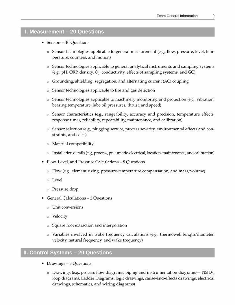
I . Measurement – 20 Questions
• Sensors – 10 Questions
Sensor technologies applicable to general measurement (e.g., flow, pressure, level, tem-perature, counters, and motion)
Sensor technologies applicable to general analytical instruments and sampling systems (e.g., pH, ORP, density, O2, conductivity, effects of sampling systems, and GC)
Grounding, shielding, segregation, and alternating current (AC) coupling
Sensor technologies applicable to fire and gas detection
Sensor technologies applicable to machinery monitoring and protection (e.g., vibration, bearing temperature, lube oil pressures, thrust, and speed)
Sensor characteristics (e.g., rangeability, accuracy and precision, temperature effects, response times, reliability, repeatability, maintenance, and calibration)
Sensor selection (e.g., plugging service, process severity, environmental effects and con-straints, and costs)
Material compatibility
Installation details (e.g., process, pneumatic, electrical, location, maintenance, and calibration)
• Flow, Level, and Pressure Calculations – 8 Questions
Flow (e.g., element sizing, pressure-temperature compensation, and mass/volume)
Level
Pressure drop
• General Calculations – 2 Questions
Unit conversions
Velocity
Square root extraction and interpolation
Variables involved in wake frequency calculations (e.g., thermowell length/diameter,velocity, natural frequency, and wake frequency)
II . Control Systems – 20 Questions
• Drawings – 3 Questions
Drawings (e.g., process flow diagrams, piping and instrumentation diagrams— P&IDs,loop diagrams, Ladder Diagrams, logic drawings, cause-and-effects drawings, electrical drawings, schematics, and wiring diagrams)
15
3 Reference Materials for the Exam
Recommended Books and Materials to Take to the Exam
I have included a review of all subject material that is in the NCEES PE/CSE exam specifications and almost any data you may need to look up for questions on the exam.
The list of recommended books and materials for testing is provided to help you pass the CSE exam. Use the materials with which you are most comfortable. A substitution with the same mate-rial and information may be used.
The list of recommended books and materials for additional study can be helpful in the review of subjects and preparation for the exam. See the International Society of Automation (ISA) web-site (www.isa.org) for more books that may give you knowledge and deeper insight into various subjects in instrumentation and control systems.
Remember to keep the review simple. The test is not focused on control systems theory stud-ies, but rather on general functional design. Again, keep your studies simple and practical; control systems theory will encompass only about 3% of the exam.
National Council ofExaminers forEngineering and SurveyingNonprofit organization
The National Council of Examiners for Engineering and Surveying is a national nonprofit organization composed of engineering and land surveying licensing boards representing all US states and territories.
Founded: 1920
NCEES on Wikipedia
NCEES on LinkedIn
Click on any link above to visit the site.
19
4 Measurement Standards and Terminology
Overview of Process Measurement, Control, and Calibration
The process control industry covers a wide variety of applications: petrochemical, pharmaceu-tical, pulp and paper, food processing, material handling, and even commercial applications. Experience designing process control systems is almost a necessity to pass the CSE PE exam.
Process control in a plant can include discrete logic, such as relay logic or a programmable logic controller (PLC); analog control, such as single-loop control or a distributed control system (DCS); and pneumatic, hydraulic, and electrical systems. The CSE must be versatile and have a broad range of understanding of the engineering sciences. The CSE is typically referred to as instrumentation and electrical (I&E), though the CSE must have in-depth knowledge of mechanical and process systems.
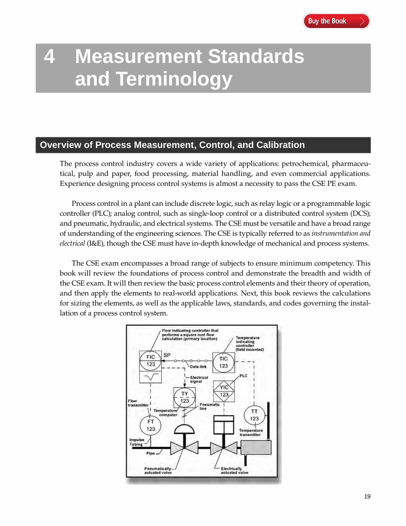
The CSE exam encompasses a broad range of subjects to ensure minimum competency. This book will review the foundations of process control and demonstrate the breadth and width of the CSE exam. It will then review the basic process control elements and their theory of operation, and then apply the elements to real-world applications. Next, this book reviews the calculations for sizing the elements, as well as the applicable laws, standards, and codes governing the instal-lation of a process control system.
20 Control Systems Engineering Exam Reference Manual
Process Signal and Calibration Terminology
The most important terms in process measurement and calibration are range, span, zero, accuracy, and repeatability. Let us start by first defining span, range, lower range value (LRV), upper range value (URV), zero, elevated zero, and suppressed zero.
Definition of the Range of an Instrument
The range is the region in which a quantity can be measured, received, or transmitted, by an ele-ment, controller, or final control device. The range can usually be adjusted and is expressed by stating the lower and upper range values.
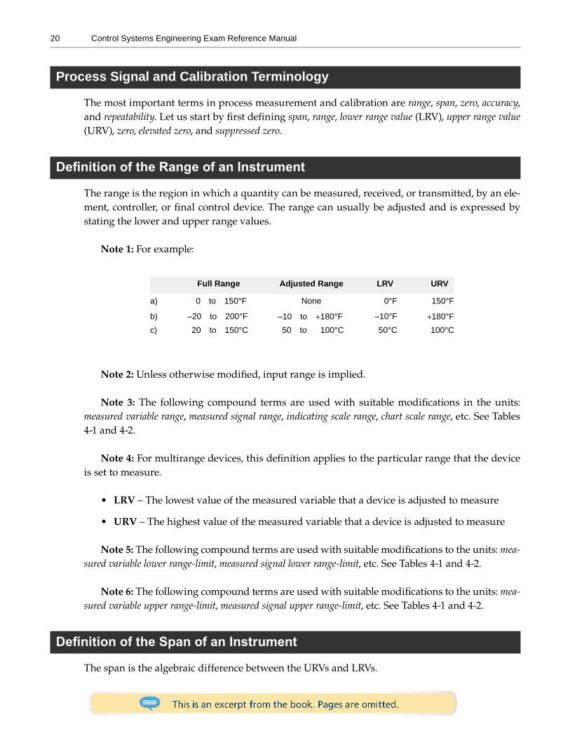
Note 1: For example:
Note 2: Unless otherwise modified, input range is implied.
Note 3: The following compound terms are used with suitable modifications in the units: measured variable range, measured signal range, indicating scale range, chart scale range, etc. See Tables 4-1 and 4-2.
Note 4: For multirange devices, this definition applies to the particular range that the device is set to measure.
• LRV – The lowest value of the measured variable that a device is adjusted to measure
• URV – The highest value of the measured variable that a device is adjusted to measure
Note 5: The following compound terms are used with suitable modifications to the units: mea-sured variable lower range-limit, measured signal lower range-limit, etc. See Tables 4-1 and 4-2.
Note 6: The following compound terms are used with suitable modifications to the units: mea-sured variable upper range-limit, measured signal upper range-limit, etc. See Tables 4-1 and 4-2.
Definition of the Span of an Instrument
The span is the algebraic difference between the URVs and LRVs.
Full Range Adjusted Range LRV URV
a) 0 to 150°F None 0°F 150°F
b) –20 to 200°F –10 to +180°F –10°F +180°Fc) 20 to 150°C 50 to 100°C 50°C 100°C
25
5 Fluid Mechanics in Process Control
Relationship of Pressure and Flow
In a pipe, the static pressure distributed across the pipe is even during no flow or deadheaded with pump. The pressure at both ends of the pipe is the same because the total energy in the system is at equilibrium. As the fluid flows, it is accelerated through the pipe. There is a pressure drop across the pipe. The static pressure is a measurement of the potential energy in the fluid. It is changed to the form of kinetic energy and is used up in the form of heat and vibration doing work on the pipe to overcome the friction of the pipe.
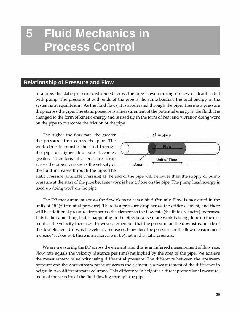
The higher the flow rate, the greater the pressure drop across the pipe. The work done to transfer the fluid through the pipe at higher flow rates becomes greater. Therefore, the pressure drop across the pipe increases as the velocity of the fluid increases through the pipe. The static pressure (available pressure) at the end of the pipe will be lower than the supply or pump pressure at the start of the pipe because work is being done on the pipe. The pump head energy is used up doing work on the pipe.
The DP measurement across the flow element acts a bit differently. Flow is measured in the units of DP (differential pressure). There is a pressure drop across the orifice element, and there will be additional pressure drop across the element as the flow rate (the fluid’s velocity) increases. This is the same thing that is happening in the pipe, because more work is being done on the ele-ment as the velocity increases. However, remember that the pressure on the downstream side of the flow element drops as the velocity increases. How does the pressure for the flow measurement increase? It does not; there is an increase in DP, not in the static pressure.
We are measuring the DP across the element, and this is an inferred measurement of flow rate. Flow rate equals the velocity (distance per time) multiplied by the area of the pipe. We achieve the measurement of velocity using differential pressure. The difference between the upstream pressure and the downstream pressure across the element is a measurement of the difference in height in two different water columns. This difference in height is a direct proportional measure-ment of the velocity of the fluid flowing through the pipe.
26 Control Systems Engineering Exam Reference Manual
The pump endows potential energy into the fluid and accelerates the fluid upward into a measurable column of water. The water column is typically measured in feet of head pressure but can be measured in pounds per square inch (psi). The water is constantly “falling” down the pipe toward the other end of the pipe, and the pump must constantly accelerate the water upward against the pull of gravity to keep the water column up in the air. The potential energy endowed into the water column turns into kinetic energy as the water column falls.
The kinetic energy is used to overcome the resistance of the pipe and the work done on the pipe as the fluid flows to the other end. If there is energy left over in the fluid, it is again trans-formed into potential energy at the other end of the pipe, as an available pressure at the end of the pipe. This potential energy left over can now fall through a pipe, device, or piece of equipment and do work, finally resting at a state of equilibrium. At this point, all the energy endowed into the fluid by the pump will be used up.
Note: The image at the right shows that the pump must develop enough head to raise the fluid to the pipe’s top elevation plus enough head to overcome the friction loss of the piping (suction and discharge). We will also need to add head for any differential pressure across the valve and the orifice or head type meter.
The velocity of the fluid is measured as the fluid falls: V2 = 2gH, where H is the height in feet (the head). The volumetric flow rate can then be an inferred measurement of the height of the water column. By knowing the size of the pipe, the coefficient of the orifice, and the properties of the fluid, we can accurately measure the volumetric flow rate of the fluid.
As the fluid flows through the opening of the orifice restriction, kinetic energy is transformed into potential energy in the form of a difference of water column on each side of the restriction orifice element. The height of the water column is the “scaled” velocity of the fluid through the pipe. Remember that the slower the fluid travels, the less work it has to do. The fluid has to acceler-ate through the small opening in the orifice to maintain the same mass flow rate through the pipe. Mass in must equal mass out.
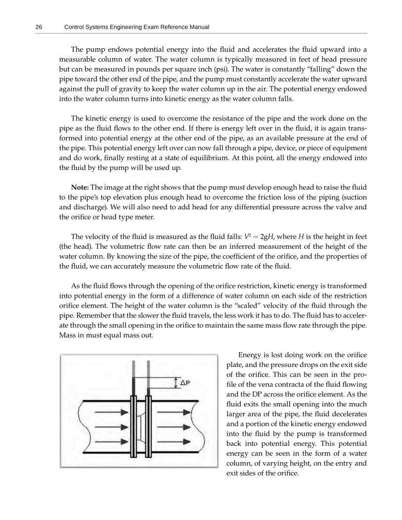
Energy is lost doing work on the orifice plate, and the pressure drops on the exit side of the orifice. This can be seen in the pro-file of the vena contracta of the fluid flowing and the DP across the orifice element. As the fluid exits the small opening into the much larger area of the pipe, the fluid decelerates and a portion of the kinetic energy endowed into the fluid by the pump is transformed back into potential energy. This potential energy can be seen in the form of a water column, of varying height, on the entry and exit sides of the orifice.
27Fluid Mechanics in Process Control
If the pipe were blocked at the exit end, the water would squirt out the taps on both sides of the orifice and the two water columns of equal height would become obvious. Again, as the fluid starts to accelerate through the pipe and through the orifice, the fluid’s potential energy tends to change back into kinetic energy to do work. This means the water columns start to fall on both side of the orifice. The exit side will fall even more than the entrance side, because work is done on the orifice restriction element as the flow rate increases. The difference in height the column falls on the exit side compared to the upstream column is its scaled velocity of the flow rate. The higher the fluid’s velocity, the more work is done on the orifice and the pressure drops even more on the exit side of the orifice. This gives a greater DP across the orifice. Note that as the pressure drops in the pipe due to increased velocity, the DP at the measurement meter becomes greater. This is because the total system pressure (total hydraulic head) is decreasing by doing work on the pipe, and the potential energy (pressure head) is being transformed back to kinetic energy (velocity head) to do the work.
The lower the fluid’s velocity through the orifice, the higher the pressure on the exit side of the orifice. This means there is less difference between the pressure on the high side (entry side) water column and the low side pressure (exit side) water column. Therefore, there is less measured DP across the orifice when the fluid decelerates, even though the pressure increased on the exit side of the orifice and everywhere in the pipe system.
Note that as the fluid flow approaches a stop, the two water columns are almost even in height. The DP becomes almost nothing. The static pressure on the exit side of the orifice, which repre-sents the potential energy in the fluid, becomes greater. The pipe system will try to reach equilib-rium or uniform distribution of static pressure across the pipe system as the work across the pipe becomes less and less. The kinetic energy will change back into potential energy.
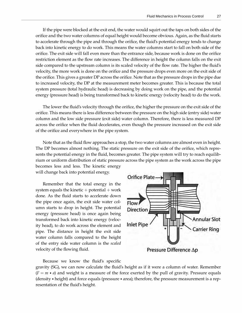
Remember that the total energy in the system equals the kinetic + potential + work done. As the fluid starts to accelerate down the pipe once again, the exit side water col-umn starts to drop in height. The potential energy (pressure head) is once again being transformed back into kinetic energy (veloc-ity head), to do work across the element and pipe. The distance in height the exit side water column falls compared to the height of the entry side water column is the scaled velocity of the flowing fluid.
Because we know the fluid’s specific gravity (SG), we can now calculate the fluid’s height as if it were a column of water. Remember (F = m • a) and weight is a measure of the force exerted by the pull of gravity. Pressure equals (density • height) and force equals (pressure • area); therefore, the pressure measurement is a rep-resentation of the fluid’s height.
37
6 Temperature Measurement and Calibration
Temperature Measurement Devices and Calibration
In the process industry, temperature measurements are typically made with thermocouples, resis-tance temperature detectors (RTDs), and industrial thermometers. Industrial thermometers are typically liquid (class I), vapor (class II), or gas (class III).
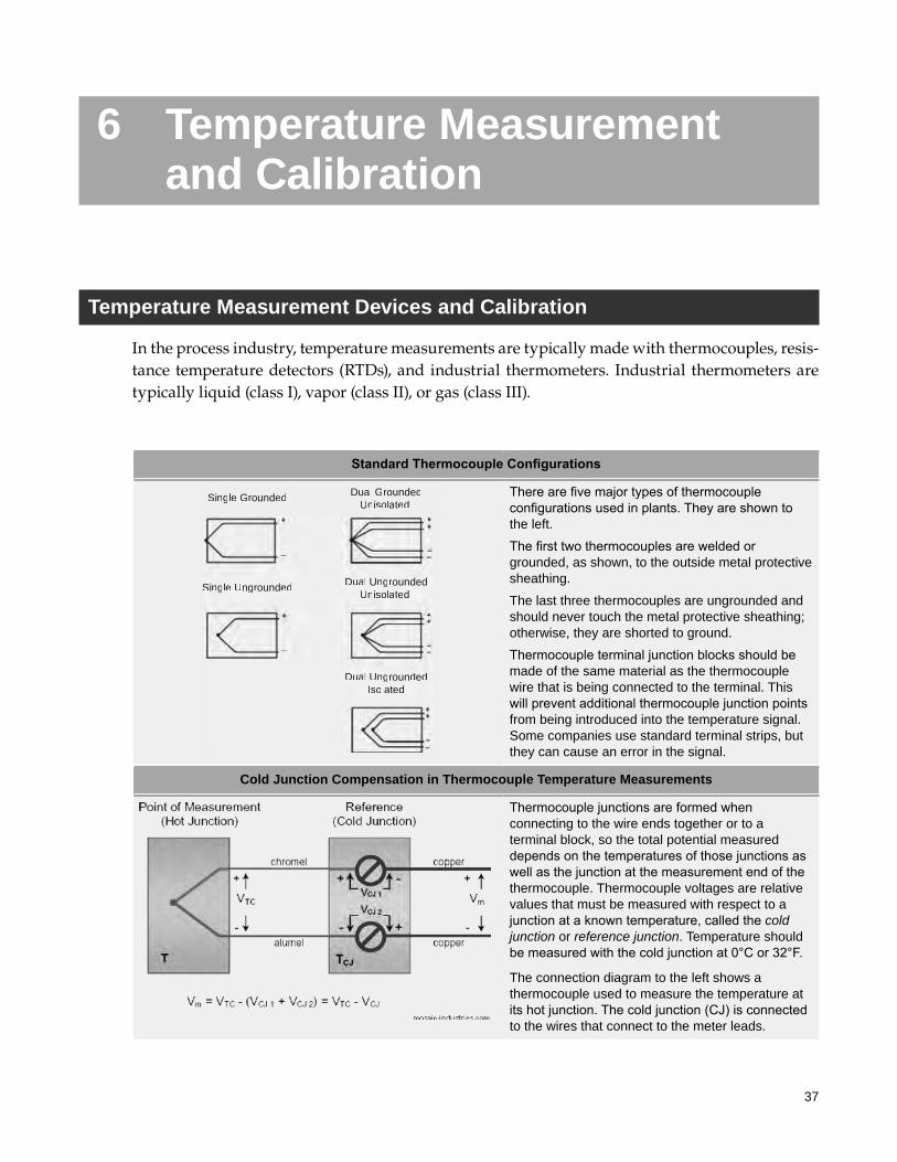
Standard Thermocouple Configurations
Single Grounded Dual GroundedUnisolated
SSingle Ungrounded Dual UngroundedUnisolated
Dual UngroundedIsolated
There are five major types of thermocouple configurations used in plants. They are shown to the left.The first two thermocouples are welded or grounded, as shown, to the outside metal protective sheathing.The last three thermocouples are ungrounded and should never touch the metal protective sheathing; otherwise, they are shorted to ground.Thermocouple terminal junction blocks should be made of the same material as the thermocouple wire that is being connected to the terminal. This will prevent additional thermocouple junction points from being introduced into the temperature signal. Some companies use standard terminal strips, but they can cause an error in the signal.
Cold Junction Compensation in Thermocouple Temperature Measurements
Thermocouple junctions are formed when connecting to the wire ends together or to a terminal block, so the total potential measured depends on the temperatures of those junctions as well as the junction at the measurement end of the thermocouple. Thermocouple voltages are relative values that must be measured with respect to a junction at a known temperature, called the cold junction or reference junction. Temperature should be measured with the cold junction at 0°C or 32°F.
The connection diagram to the left shows a thermocouple used to measure the temperature at its hot junction. The cold junction (CJ) is connected to the wires that connect to the meter leads.
38 Control Systems Engineering Exam Reference Manual
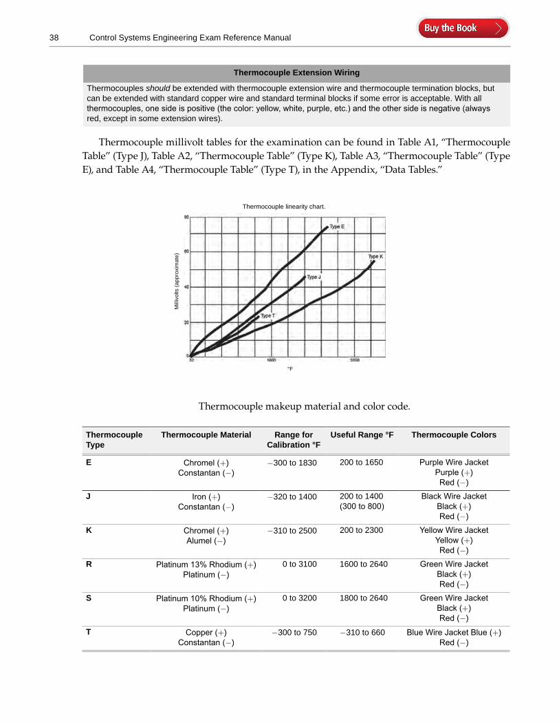
Thermocouple millivolt tables for the examination can be found in Table A1, “Thermocouple Table” (Type J), Table A2, “Thermocouple Table” (Type K), Table A3, “Thermocouple Table” (Type E), and Table A4, “Thermocouple Table” (Type T), in the Appendix, “Data Tables.”
Thermocouple linearity chart.
°F
Mill
ivol
ts (
appr
oxim
ate)
Thermocouple makeup material and color code.
Thermocouple Type
Thermocouple Material Range for Calibration °F
Useful Range °F Thermocouple Colors
E Chromel (+) Constantan (−)
−300 to 1830 200 to 1650 Purple Wire JacketPurple (+)Red (−)
J Iron (+) Constantan (−)
−320 to 1400 200 to 1400 (300 to 800)
Black Wire JacketBlack (+)Red (−)
K Chromel (+)Alumel (−)
−310 to 2500 200 to 2300 Yellow Wire JacketYellow (+)Red (−)
R Platinum 13% Rhodium (+) Platinum (−)
0 to 3100 1600 to 2640 Green Wire JacketBlack (+)Red (−)
S Platinum 10% Rhodium (+) Platinum (−)
0 to 3200 1800 to 2640 Green Wire JacketBlack (+)Red (−)
T Copper (+)Constantan (−)
−300 to 750 −310 to 660 Blue Wire Jacket Blue (+) Red (−)
Thermocouple Extension Wiring
Thermocouples should be extended with thermocouple extension wire and thermocouple termination blocks, but can be extended with standard copper wire and standard terminal blocks if some error is acceptable. With all thermocouples, one side is positive (the color: yellow, white, purple, etc.) and the other side is negative (always red, except in some extension wires).

39Temperature Measurement and Calibration
Sample Problem: What is the millivolt (mV) output of a Type J thermocouple at 218°F and referenced to a 32°F electronic ice bath?
Find the nearest temperature in Table A1, “Thermocouple Table” (Type J), in the Appendix of this guide.
The nearest temperature in the first column is 210. Look at the column headers at the bottom of the chart. Find the column header labeled 8. Follow the column up to the row with the 210 value. Where they meet is a total of 210°F + 8°F = 218°F.
Read the value of mV. The answer is 5.45 mV.
Thermocouple − Worked Examples (How to Read the Thermocouple Tables)
Resistance Temperature Detector
The process control industry also uses RTDs for many applications, for example, when precise temperature measurement is needed, such as mass flow measurements or critical temperature measurements of motor bearings.
Sample Problem: What is the millivolt (mV) output of a type K thermocouple at 672°F from the data given? Assume the thermocouple is linear.
Given:670°F = 14.479 mV672°F = mV680°F = 14.713 mV
Interpolate the mV value for the desired temperature as follows:
Interpolation:
output desired
mV
=
deg deg
deg deg
−
−
lower value
upper value llower valueupper value lower value
( )
mV mV−
+ mV lower values
Therefore, the output (mV) for 672°F:
14 526672 670680 670
14 713 14 479 14. . . .=−−
−( )
+ 4479
The output at 672°F is 14.526 mV.
This can be verified in Table A2, “Thermocouple Table” (Type K), in the Appendix.
49
7 Pressure Measurement and Calibration
Pressure Measurement and Head Pressure
Pressure is typically measured in two different forms, pounds per square inch (psi) or head pressure. Head pressure is measured in inches or feet of water column (H2O).
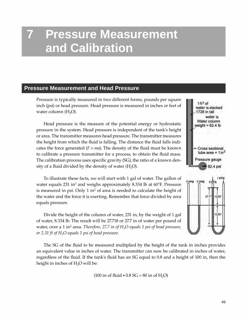
Head pressure is the measure of the potential energy or hydrostatic pressure in the system. Head pressure is independent of the tank’s height or area. The transmitter measures head pressure. The transmitter measures the height from which the fluid is falling. The distance the fluid falls indi-cates the force generated (F = ma). The density of the fluid must be known to calibrate a pressure transmitter for a process, to obtain the fluid mass. The calibration process uses specific gravity (SG), the ratio of a known den-sity of a fluid divided by the density of water (H2O).
To illustrate these facts, we will start with 1 gal of water. The gallon of water equals 231 in3 and weighs approximately 8.334 lb at 60°F. Pressure is measured in psi. Only 1 in2 of area is needed to calculate the height of the water and the force it is exerting. Remember that force divided by area equals pressure.
Divide the height of the column of water, 231 in, by the weight of 1 gal of water, 8.334 lb. The result will be 27.718 or 27.7 in of water per pound of water, over a 1 in2 area. Therefore, 27.7 in of H2O equals 1 psi of head pressure, or 2.31 ft of H2O equals 1 psi of head pressure.
The SG of the fluid to be measured multiplied by the height of the tank in inches provides an equivalent value in inches of water. The transmitter can now be calibrated in inches of water, regardless of the fluid. If the tank’s fluid has an SG equal to 0.8 and a height of 100 in, then the height in inches of H2O will be:
(100 in of fluid • 0.8 SG = 80 in of H2O)
50 Control Systems Engineering Exam Reference Manual
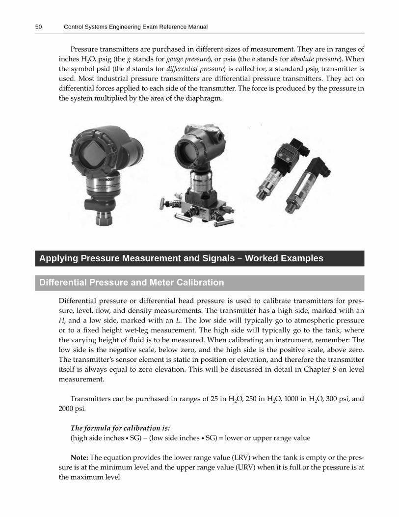
Pressure transmitters are purchased in different sizes of measurement. They are in ranges of inches H2O, psig (the g stands for gauge pressure), or psia (the a stands for absolute pressure). When the symbol psid (the d stands for differential pressure) is called for, a standard psig transmitter is used. Most industrial pressure transmitters are differential pressure transmitters. They act on differential forces applied to each side of the transmitter. The force is produced by the pressure in the system multiplied by the area of the diaphragm.
Applying Pressure Measurement and Signals – Worked Examples
Differential Pressure and Meter Calibration
Differential pressure or differential head pressure is used to calibrate transmitters for pres-sure, level, flow, and density measurements. The transmitter has a high side, marked with an H, and a low side, marked with an L. The low side will typically go to atmospheric pressure or to a fixed height wet-leg measurement. The high side will typically go to the tank, where the varying height of fluid is to be measured. When calibrating an instrument, remember: The low side is the negative scale, below zero, and the high side is the positive scale, above zero. The transmitter’s sensor element is static in position or elevation, and therefore the transmitter itself is always equal to zero elevation. This will be discussed in detail in Chapter 8 on level measurement.
Transmitters can be purchased in ranges of 25 in H2O, 250 in H2O, 1000 in H2O, 300 psi, and 2000 psi.
The formula for calibration is:(high side inches • SG) - (low side inches • SG) = lower or upper range value
Note: The equation provides the lower range value (LRV) when the tank is empty or the pres-sure is at the minimum level and the upper range value (URV) when it is full or the pressure is at the maximum level.
51Pressure Measurement and Calibration
Pressure Change in a Pipe for a Given Flow Rate
On the CSE exam, you will be asked to correlate signals and measurements using flow, pressure and the output in 4–20 mA signals. A change in flow in a pipe will cause a change in the head pressure across the pipe and measurement element. If the flow decreases in the pipe, the pressure in the pipe will increase at any point along the pipe.
If the flow rate increases, the pressure in the piping system decreases. If the flow rate decreases, the pressure in the piping system increases. This is because the total head of the system remains constant due to the head pressure developed by the pump. The total energy head being endowed into the pump and piping system remains constant. This is the case with a pump at a constant speed; two pressure gauges, one at each end of the pipe; and a hand valve at the end of the pipe.
h F h F hFF
h1 12
2 22
11
2
2
2=
=
Sample Problem: A pressure gauge is reading 25 psig. It is attached to a tank filled with a fluid. The bottom of the tank is 65 ft above the ground. The pressure gauge is 5 ft above the ground. The fluid has a specific gravity of 0.7. What is the level of the fluid in the tank?
First, convert the psig measurement to feet of head measurement.
25 psig • 2.31 ft per psi = 57.75 ft of H2O
Next, find the elevation of the bottom of the tank in relation to the elevation of the pressure gauge. Tank bottom in feet – pressure gauge elevation in feet = the height in feet to the bottom of the tank
65 ft - 5 ft = 60 ft of head to the bottom of the tank
Note: Head is always measured in the standard of inches or feet of water column (wc).
Multiply the head between the bottom of the tank and the pressure gauge times the SG to get the head equal to H2O.
60 ft of fluid • 0.7 SG = 42 ft H2O to bottom of tank from the pressure gauge
Next, subtract the height from the pressure gauge to the bottom of the tank in feet of H2O from the total height of fluid in feet of in H2O above the pressure gauge to find the height of the fluid in the tank in H2O.
(57.75 ft of H2O total head) - (42 ft of H2O below the tank) = feet of fluid in H2O in the tank(57.75 ft total) - (42 ft to bottom tank from the pressure gauge) = 15.75 ft in H2O in the tank
Next, convert height in feet of H2O to height of fluid with an SG of 0.7.
15.75 ft of H2O/0.7 SG = 22.5 ft of total height of the fluid column in the tank
55
8 Level Measurement and Calibration
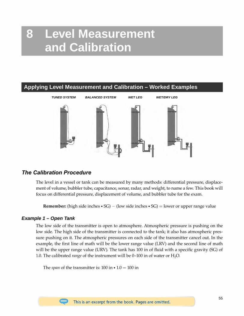
Applying Level Measurement and Calibration – Worked ExamplesTUNED SYSTEM BALANCED SYSTEM WET LEG WET/DRY LEG
The Calibration ProcedureThe level in a vessel or tank can be measured by many methods: differential pressure, displace-ment of volume, bubbler tube, capacitance, sonar, radar, and weight, to name a few. This book will focus on differential pressure, displacement of volume, and bubbler tube for the exam.
Remember: (high side inches • SG) − (low side inches • SG) = lower or upper range value
Example 1 – Open TankThe low side of the transmitter is open to atmosphere. Atmospheric pressure is pushing on the low side. The high side of the transmitter is connected to the tank; it also has atmospheric pres-sure pushing on it. The atmospheric pressures on each side of the transmitter cancel out. In the example, the first line of math will be the lower range value (LRV) and the second line of math will be the upper range value (URV). The tank has 100 in of fluid with a specific gravity (SG) of 1.0. The calibrated range of the instrument will be 0–100 in of water or H2O.
The span of the transmitter is: 100 in • 1.0 = 100 in
56 Control Systems Engineering Exam Reference Manual
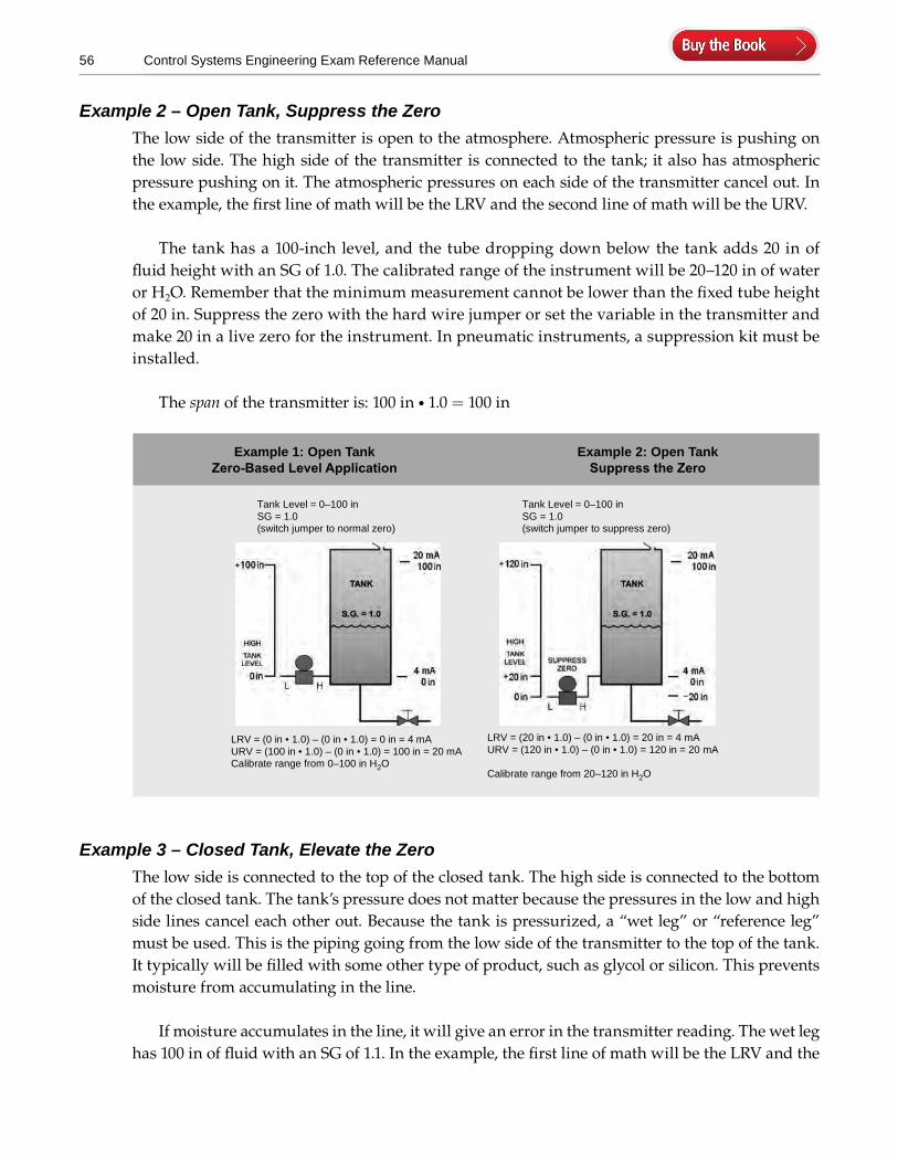
Example 2 – Open Tank, Suppress the ZeroThe low side of the transmitter is open to the atmosphere. Atmospheric pressure is pushing on the low side. The high side of the transmitter is connected to the tank; it also has atmospheric pressure pushing on it. The atmospheric pressures on each side of the transmitter cancel out. In the example, the first line of math will be the LRV and the second line of math will be the URV.
The tank has a 100-inch level, and the tube dropping down below the tank adds 20 in of fluid height with an SG of 1.0. The calibrated range of the instrument will be 20–120 in of water or H2O. Remember that the minimum measurement cannot be lower than the fixed tube height of 20 in. Suppress the zero with the hard wire jumper or set the variable in the transmitter and make 20 in a live zero for the instrument. In pneumatic instruments, a suppression kit must be installed.
The span of the transmitter is: 100 in • 1.0 = 100 in
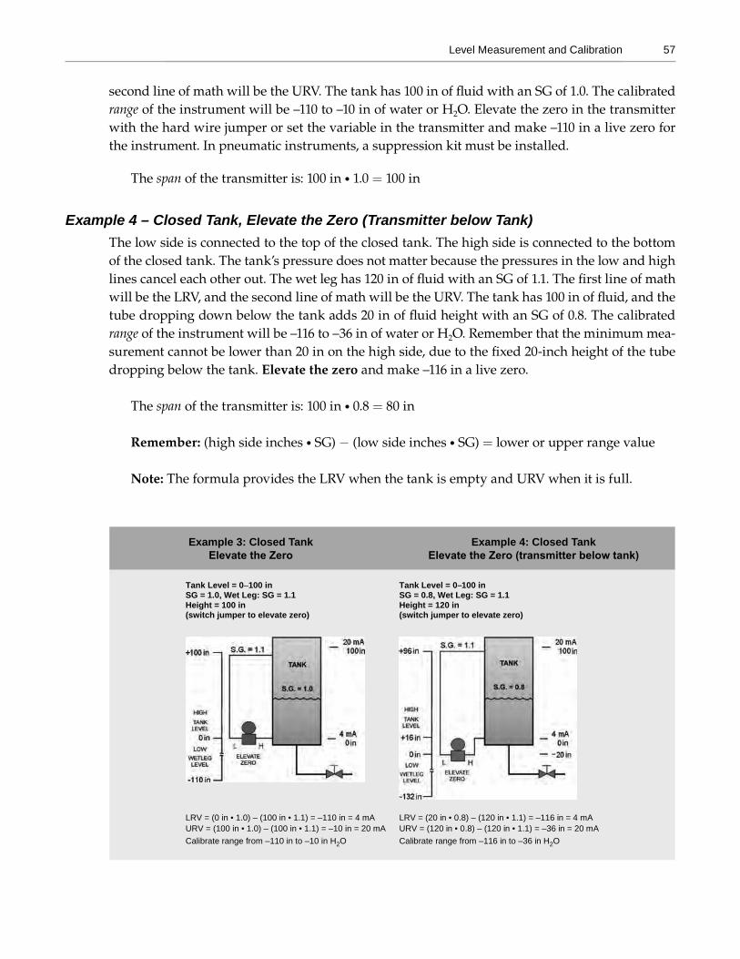
Example 3 – Closed Tank, Elevate the ZeroThe low side is connected to the top of the closed tank. The high side is connected to the bottom of the closed tank. The tank’s pressure does not matter because the pressures in the low and high side lines cancel each other out. Because the tank is pressurized, a “wet leg” or “reference leg” must be used. This is the piping going from the low side of the transmitter to the top of the tank. It typically will be filled with some other type of product, such as glycol or silicon. This prevents moisture from accumulating in the line.
If moisture accumulates in the line, it will give an error in the transmitter reading. The wet leg has 100 in of fluid with an SG of 1.1. In the example, the first line of math will be the LRV and the
Example 1: Open Tank Zero-Based Level Application
Example 2: Open Tank Suppress the Zero
Tank Level = 0–100 inSG = 1.0(switch jumper to normal zero)
LRV = (0 in • 1.0) – (0 in • 1.0) = 0 in = 4 mAURV = (100 in • 1.0) – (0 in • 1.0) = 100 in = 20 mACalibrate range from 0–100 in H2O
Tank Level = 0–100 inSG = 1.0(switch jumper to suppress zero)
LRV = (20 in • 1.0) – (0 in • 1.0) = 20 in = 4 mAURV = (120 in • 1.0) – (0 in • 1.0) = 120 in = 20 mA
Calibrate range from 20–120 in H2O
57Level Measurement and Calibration
second line of math will be the URV. The tank has 100 in of fluid with an SG of 1.0. The calibrated range of the instrument will be –110 to –10 in of water or H2O. Elevate the zero in the transmitter with the hard wire jumper or set the variable in the transmitter and make –110 in a live zero for the instrument. In pneumatic instruments, a suppression kit must be installed.
The span of the transmitter is: 100 in • 1.0 = 100 in
Example 4 – Closed Tank, Elevate the Zero (Transmitter below Tank)The low side is connected to the top of the closed tank. The high side is connected to the bottom of the closed tank. The tank’s pressure does not matter because the pressures in the low and high lines cancel each other out. The wet leg has 120 in of fluid with an SG of 1.1. The first line of math will be the LRV, and the second line of math will be the URV. The tank has 100 in of fluid, and the tube dropping down below the tank adds 20 in of fluid height with an SG of 0.8. The calibrated range of the instrument will be –116 to –36 in of water or H2O. Remember that the minimum mea-surement cannot be lower than 20 in on the high side, due to the fixed 20-inch height of the tube dropping below the tank. Elevate the zero and make –116 in a live zero.
The span of the transmitter is: 100 in • 0.8 = 80 in
Remember: (high side inches • SG) − (low side inches • SG) = lower or upper range value
Note: The formula provides the LRV when the tank is empty and URV when it is full.
Example 3: Closed Tank Elevate the Zero
Example 4: Closed Tank Elevate the Zero (transmitter below tank)
Tank Level = 0–100 inSG = 1.0, Wet Leg: SG = 1.1 Height = 100 in(switch jumper to elevate zero)
LRV = (0 in • 1.0) – (100 in • 1.1) = –110 in = 4 mAURV = (100 in • 1.0) – (100 in • 1.1) = –10 in = 20 mACalibrate range from –110 in to –10 in H2O
Tank Level = 0–100 inSG = 0.8, Wet Leg: SG = 1.1Height = 120 in(switch jumper to elevate zero)
LRV = (20 in • 0.8) – (120 in • 1.1) = –116 in = 4 mAURV = (120 in • 0.8) – (120 in • 1.1) = –36 in = 20 mACalibrate range from –116 in to –36 in H2O
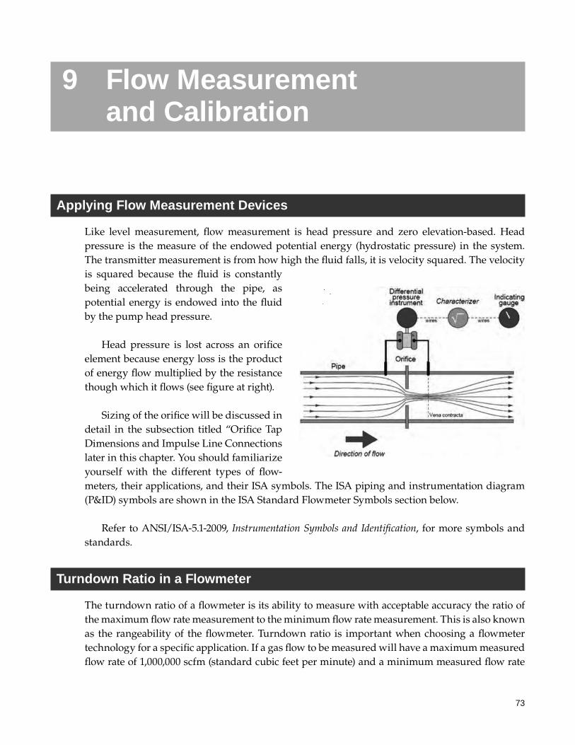
73
9 Flow Measurement and Calibration
Applying Flow Measurement Devices
Like level measurement, flow measurement is head pressure and zero elevation-based. Head pressure is the measure of the endowed potential energy (hydrostatic pressure) in the system. The transmitter measurement is from how high the fluid falls, it is velocity squared. The velocity is squared because the fluid is constantly being accelerated through the pipe, as potential energy is endowed into the fluid by the pump head pressure.
Head pressure is lost across an orifice element because energy loss is the product of energy flow multiplied by the resistance though which it flows (see figure at right).
Sizing of the orifice will be discussed in detail in the subsection titled “Orifice Tap Dimensions and Impulse Line Connections later in this chapter. You should familiarize yourself with the different types of flow-meters, their applications, and their ISA symbols. The ISA piping and instrumentation diagram (P&ID) symbols are shown in the ISA Standard Flowmeter Symbols section below.
Refer to ANSI/ISA-5.1-2009, Instrumentation Symbols and Identification, for more symbols and standards.
Turndown Ratio in a Flowmeter
The turndown ratio of a flowmeter is its ability to measure with acceptable accuracy the ratio of the maximum flow rate measurement to the minimum flow rate measurement. This is also known as the rangeability of the flowmeter. Turndown ratio is important when choosing a flowmeter technology for a specific application. If a gas flow to be measured will have a maximum measured flow rate of 1,000,000 scfm (standard cubic feet per minute) and a minimum measured flow rate
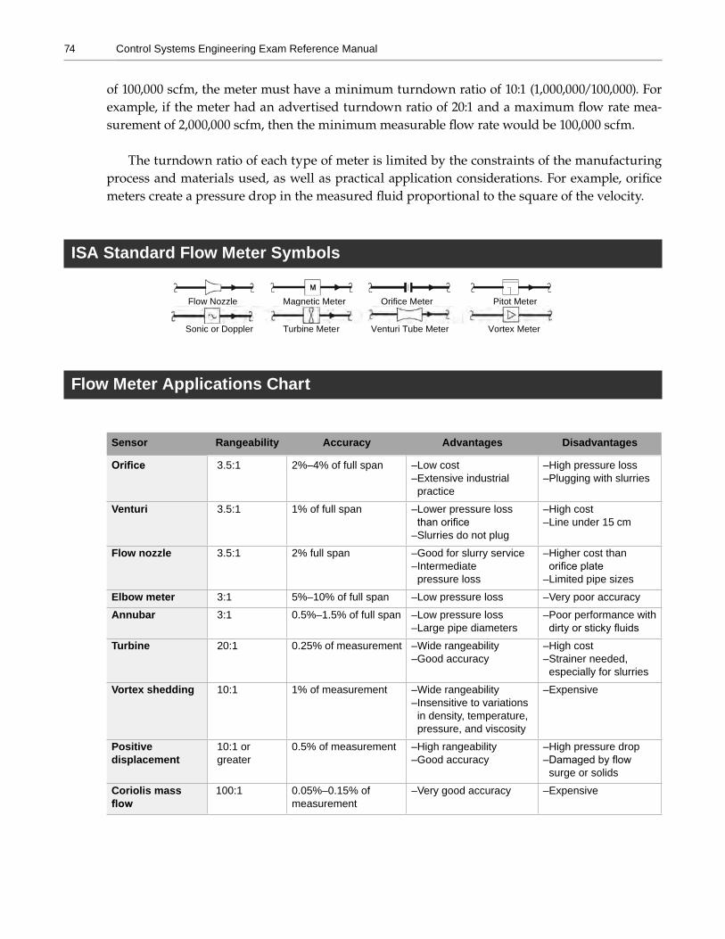
74 Control Systems Engineering Exam Reference Manual
of 100,000 scfm, the meter must have a minimum turndown ratio of 10:1 (1,000,000/100,000). For example, if the meter had an advertised turndown ratio of 20:1 and a maximum flow rate mea-surement of 2,000,000 scfm, then the minimum measurable flow rate would be 100,000 scfm.
The turndown ratio of each type of meter is limited by the constraints of the manufacturing process and materials used, as well as practical application considerations. For example, orifice meters create a pressure drop in the measured fluid proportional to the square of the velocity.
ISA Standard Flow Meter Symbols
Flow Nozzle Magnetic Meter Orifice Meter Pitot Meter
Sonic or Doppler Turbine Meter Venturi Tube Meter Vortex Meter
Flow Meter Applications Chart
Sensor Rangeability Accuracy Advantages Disadvantages
Orifice 3.5:1 2%–4% of full span –Low cost– Extensive industrial practice
–High pressure loss–Plugging with slurries
Venturi 3.5:1 1% of full span – Lower pressure lossthan orifice
–Slurries do not plug
–High cost–Line under 15 cm
Flow nozzle 3.5:1 2% full span – Good for slurry service– Intermediate pressure loss
– Higher cost thanorifice plate
–Limited pipe sizesElbow meter 3:1 5%–10% of full span –Low pressure loss –Very poor accuracyAnnubar 3:1 0.5%–1.5% of full span –Low pressure loss
–Large pipe diameters– Poor performance withdirty or sticky fluids
Turbine 20:1 0.25% of measurement –Wide rangeability –Good accuracy
–High cost– Strainer needed, especially for slurries
Vortex shedding 10:1 1% of measurement –Wide rangeability– Insensitive to variationsin density, temperature,pressure, and viscosity
–Expensive
Positive displacement
10:1 or greater
0.5% of measurement –High rangeability–Good accuracy
–High pressure drop– Damaged by flowsurge or solids
Coriolis mass flow
100:1 0.05%–0.15% of measurement
–Very good accuracy –Expensive
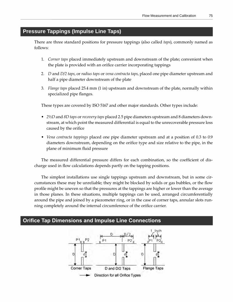
75Flow Measurement and Calibration
Pressure Tappings (Impulse Line Taps)
There are three standard positions for pressure tappings (also called taps), commonly named as follows:
1. Corner taps placed immediately upstream and downstream of the plate; convenient whenthe plate is provided with an orifice carrier incorporating tappings
2. D and D/2 taps, or radius taps or vena contracta taps, placed one pipe diameter upstream andhalf a pipe diameter downstream of the plate
3. Flange taps placed 25.4 mm (1 in) upstream and downstream of the plate, normally withinspecialized pipe flanges.
These types are covered by ISO 5167 and other major standards. Other types include:
• 2½D and 8D taps or recovery taps placed 2.5 pipe diameters upstream and 8 diameters down-stream, at which point the measured differential is equal to the unrecoverable pressure losscaused by the orifice
• Vena contracta tappings placed one pipe diameter upstream and at a position of 0.3 to 0.9diameters downstream, depending on the orifice type and size relative to the pipe, in theplane of minimum fluid pressure
The measured differential pressure differs for each combination, so the coefficient of dis-charge used in flow calculations depends partly on the tapping positions.
The simplest installations use single tappings upstream and downstream, but in some cir-cumstances these may be unreliable; they might be blocked by solids or gas bubbles, or the flow profile might be uneven so that the pressures at the tappings are higher or lower than the average in those planes. In these situations, multiple tappings can be used, arranged circumferentially around the pipe and joined by a piezometer ring, or in the case of corner taps, annular slots run-ning completely around the internal circumference of the orifice carrier.
Orifice Tap Dimensions and Impulse Line Connections
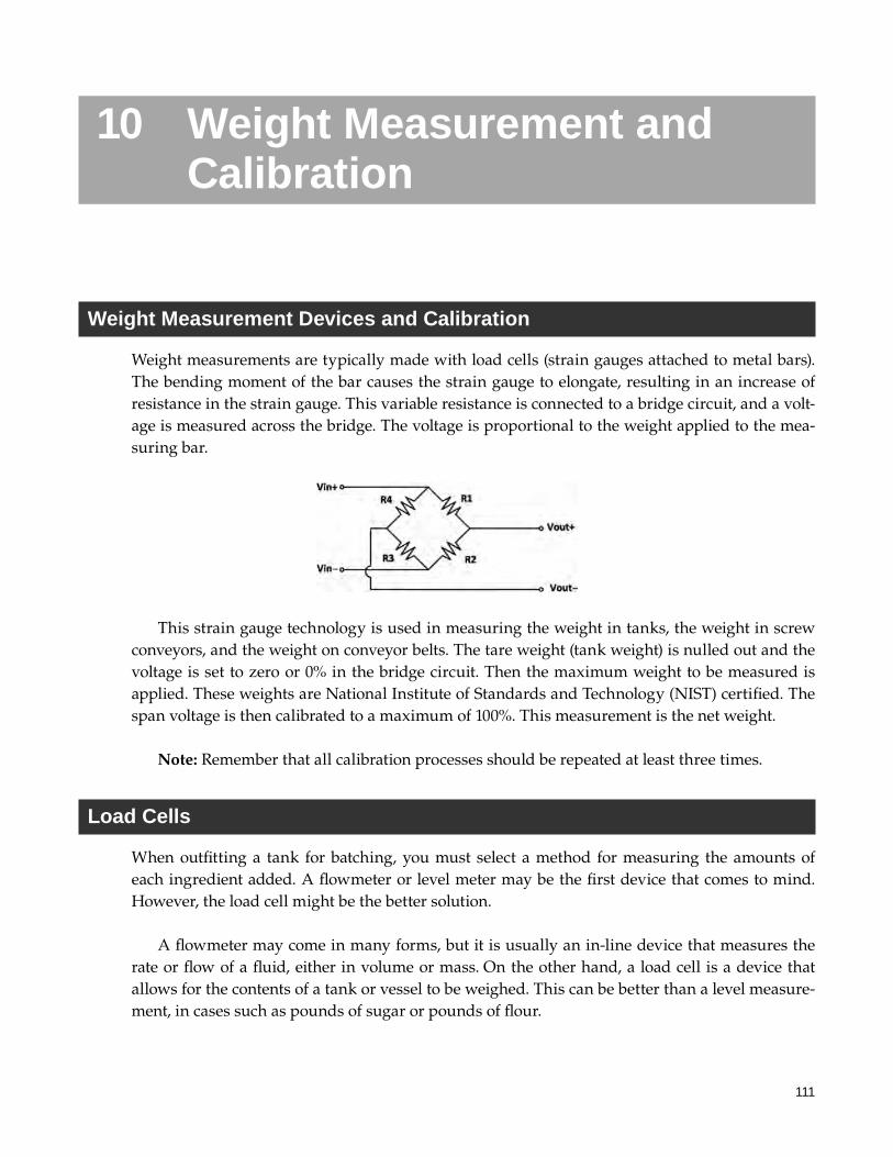
111
10 Weight Measurement and Calibration
Weight Measurement Devices and Calibration
Weight measurements are typically made with load cells (strain gauges attached to metal bars). The bending moment of the bar causes the strain gauge to elongate, resulting in an increase of resistance in the strain gauge. This variable resistance is connected to a bridge circuit, and a volt-age is measured across the bridge. The voltage is proportional to the weight applied to the mea-suring bar.
This strain gauge technology is used in measuring the weight in tanks, the weight in screw conveyors, and the weight on conveyor belts. The tare weight (tank weight) is nulled out and the voltage is set to zero or 0% in the bridge circuit. Then the maximum weight to be measured is applied. These weights are National Institute of Standards and Technology (NIST) certified. The span voltage is then calibrated to a maximum of 100%. This measurement is the net weight.
Note: Remember that all calibration processes should be repeated at least three times.
Load Cells
When outfitting a tank for batching, you must select a method for measuring the amounts of each ingredient added. A flowmeter or level meter may be the first device that comes to mind. However, the load cell might be the better solution.
A flowmeter may come in many forms, but it is usually an in-line device that measures the rate or flow of a fluid, either in volume or mass. On the other hand, a load cell is a device that allows for the contents of a tank or vessel to be weighed. This can be better than a level measure-ment, in cases such as pounds of sugar or pounds of flour.
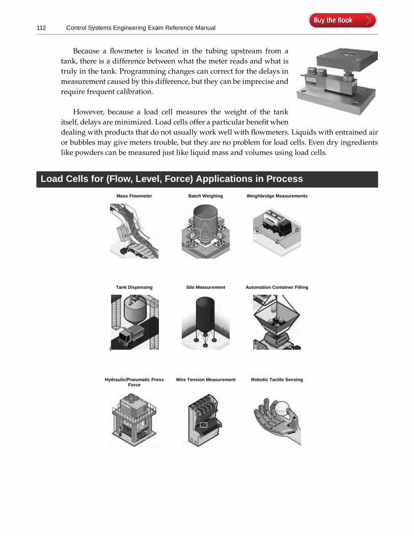
112 Control Systems Engineering Exam Reference Manual
Because a flowmeter is located in the tubing upstream from a tank, there is a difference between what the meter reads and what is truly in the tank. Programming changes can correct for the delays in measurement caused by this difference, but they can be imprecise and require frequent calibration.
However, because a load cell measures the weight of the tank itself, delays are minimized. Load cells offer a particular benefit when dealing with products that do not usually work well with flowmeters. Liquids with entrained air or bubbles may give meters trouble, but they are no problem for load cells. Even dry ingredients like powders can be measured just like liquid mass and volumes using load cells.
Load Cells for (Flow, Level, Force) Applications in ProcessMass Flowmeter Batch Weighing Weighbridge Measurements
Tank Dispensing
(
Silo Measurement Automation Container Filling
Hydraulic/Pneumatic Press Force
Wire Tension Measurement Robotic Tactile Sensing
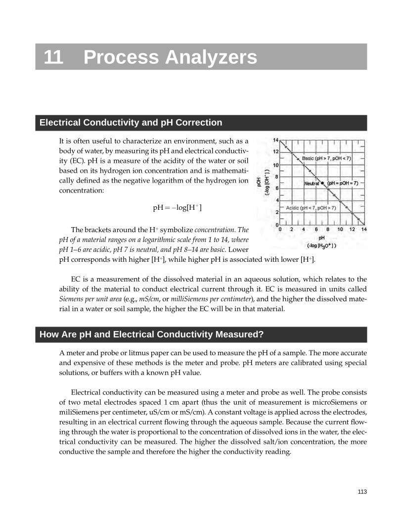
113
11 Process Analyzers
Electrical Conductivity and pH Correction
It is often useful to characterize an environment, such as a body of water, by measuring its pH and electrical conductiv-ity (EC). pH is a measure of the acidity of the water or soil based on its hydrogen ion concentration and is mathemati-cally defined as the negative logarithm of the hydrogen ion concentration:
pH log[H ]= − +
The brackets around the H+ symbolize concentration. The pH of a material ranges on a logarithmic scale from 1 to 14, where pH 1–6 are acidic, pH 7 is neutral, and pH 8–14 are basic. Lower pH corresponds with higher [H+], while higher pH is associated with lower [H+].
EC is a measurement of the dissolved material in an aqueous solution, which relates to the ability of the material to conduct electrical current through it. EC is measured in units called Siemens per unit area (e.g., mS/cm, or milliSiemens per centimeter), and the higher the dissolved mate-rial in a water or soil sample, the higher the EC will be in that material.
How Are pH and Electrical Conductivity Measured?
A meter and probe or litmus paper can be used to measure the pH of a sample. The more accurate and expensive of these methods is the meter and probe. pH meters are calibrated using special solutions, or buffers with a known pH value.
Electrical conductivity can be measured using a meter and probe as well. The probe consists of two metal electrodes spaced 1 cm apart (thus the unit of measurement is microSiemens or miliSiemens per centimeter, uS/cm or mS/cm). A constant voltage is applied across the electrodes, resulting in an electrical current flowing through the aqueous sample. Because the current flow-ing through the water is proportional to the concentration of dissolved ions in the water, the elec-trical conductivity can be measured. The higher the dissolved salt/ion concentration, the more conductive the sample and therefore the higher the conductivity reading.
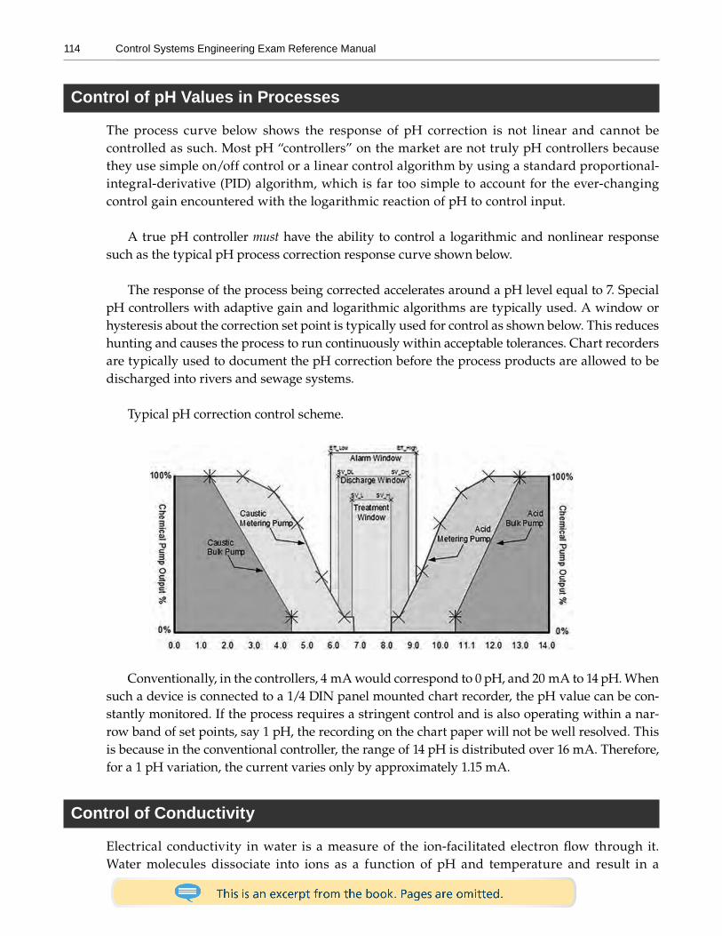
114 Control Systems Engineering Exam Reference Manual
Control of pH Values in Processes
The process curve below shows the response of pH correction is not linear and cannot be controlled as such. Most pH “controllers” on the market are not truly pH controllers because they use simple on/off control or a linear control algorithm by using a standard proportional-integral-derivative (PID) algorithm, which is far too simple to account for the ever-changing control gain encountered with the logarithmic reaction of pH to control input.
A true pH controller must have the ability to control a logarithmic and nonlinear response such as the typical pH process correction response curve shown below.
The response of the process being corrected accelerates around a pH level equal to 7. Special pH controllers with adaptive gain and logarithmic algorithms are typically used. A window or hysteresis about the correction set point is typically used for control as shown below. This reduces hunting and causes the process to run continuously within acceptable tolerances. Chart recorders are typically used to document the pH correction before the process products are allowed to be discharged into rivers and sewage systems.
Typical pH correction control scheme.
Conventionally, in the controllers, 4 mA would correspond to 0 pH, and 20 mA to 14 pH. When such a device is connected to a 1/4 DIN panel mounted chart recorder, the pH value can be con-stantly monitored. If the process requires a stringent control and is also operating within a nar-row band of set points, say 1 pH, the recording on the chart paper will not be well resolved. This is because in the conventional controller, the range of 14 pH is distributed over 16 mA. Therefore, for a 1 pH variation, the current varies only by approximately 1.15 mA.
Control of Conductivity
Electrical conductivity in water is a measure of the ion-facilitated electron flow through it. Water molecules dissociate into ions as a function of pH and temperature and result in a
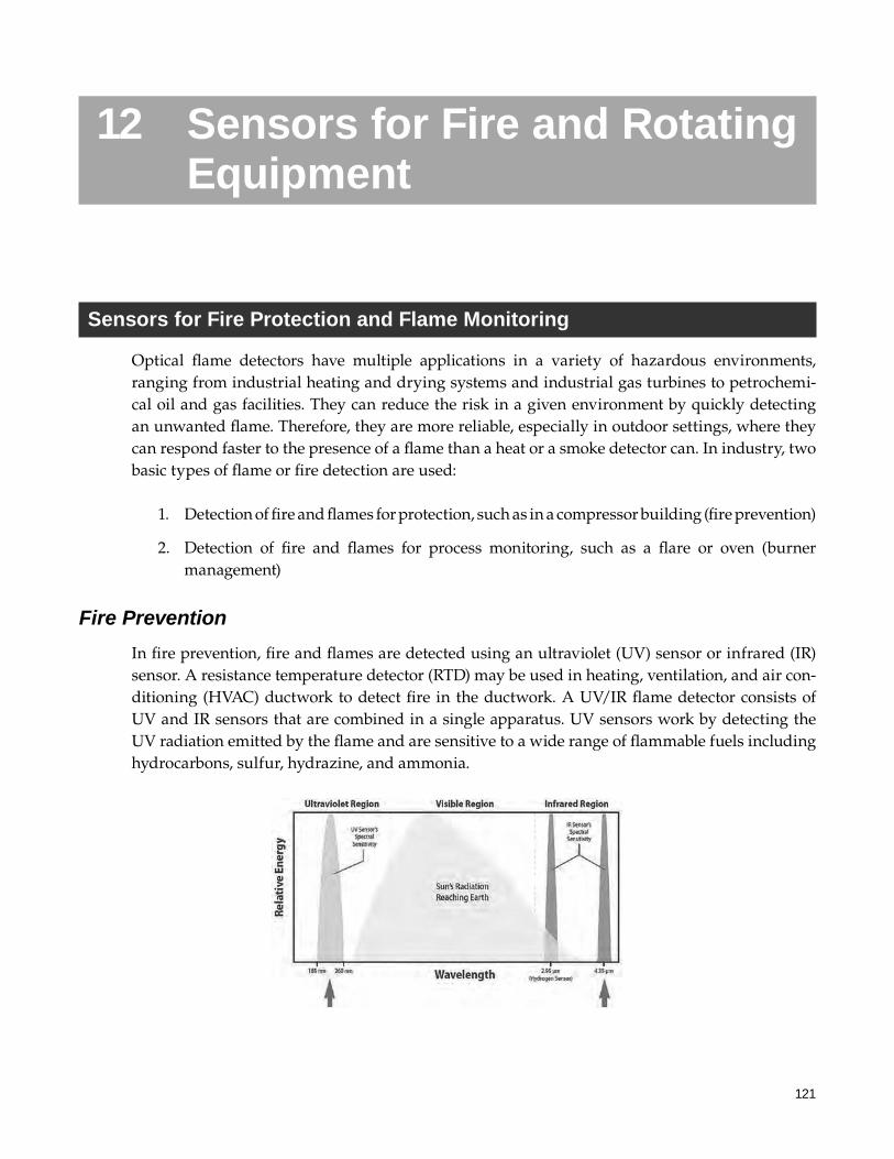
121
12 Sensors for Fire and Rotating Equipment
Sensors for Fire Protection and Flame Monitoring
Optical flame detectors have multiple applications in a variety of hazardous environments, ranging from industrial heating and drying systems and industrial gas turbines to petrochemi-cal oil and gas facilities. They can reduce the risk in a given environment by quickly detecting an unwanted flame. Therefore, they are more reliable, especially in outdoor settings, where they can respond faster to the presence of a flame than a heat or a smoke detector can. In industry, two basic types of flame or fire detection are used:
1. Detection of fire and flames for protection, such as in a compressor building (fire prevention)
2. Detection of fire and flames for process monitoring, such as a flare or oven (burnermanagement)
Fire PreventionIn fire prevention, fire and flames are detected using an ultraviolet (UV) sensor or infrared (IR) sensor. A resistance temperature detector (RTD) may be used in heating, ventilation, and air con-ditioning (HVAC) ductwork to detect fire in the ductwork. A UV/IR flame detector consists of UV and IR sensors that are combined in a single apparatus. UV sensors work by detecting the UV radiation emitted by the flame and are sensitive to a wide range of flammable fuels including hydrocarbons, sulfur, hydrazine, and ammonia.
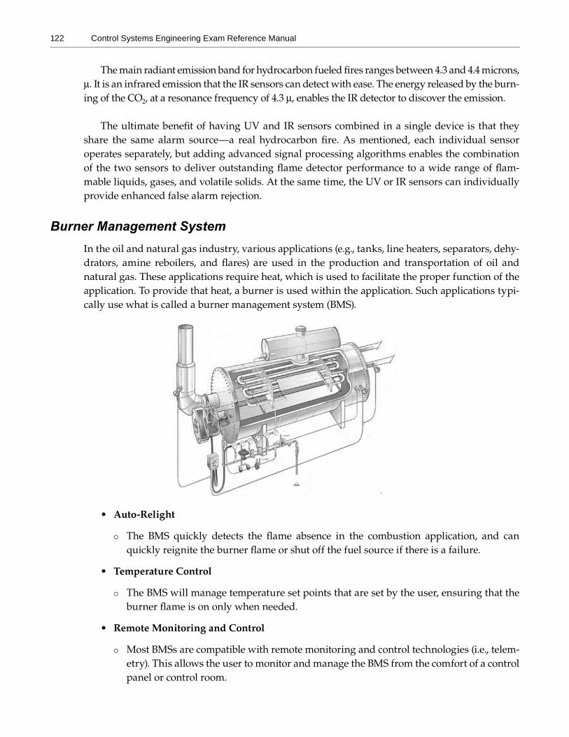
122 Control Systems Engineering Exam Reference Manual
The main radiant emission band for hydrocarbon fueled fires ranges between 4.3 and 4.4 microns, µ. It is an infrared emission that the IR sensors can detect with ease. The energy released by the burn-ing of the CO2, at a resonance frequency of 4.3 µ, enables the IR detector to discover the emission.
The ultimate benefit of having UV and IR sensors combined in a single device is that they share the same alarm source—a real hydrocarbon fire. As mentioned, each individual sensor operates separately, but adding advanced signal processing algorithms enables the combination of the two sensors to deliver outstanding flame detector performance to a wide range of flam-mable liquids, gases, and volatile solids. At the same time, the UV or IR sensors can individually provide enhanced false alarm rejection.
Burner Management SystemIn the oil and natural gas industry, various applications (e.g., tanks, line heaters, separators, dehy-drators, amine reboilers, and flares) are used in the production and transportation of oil and natural gas. These applications require heat, which is used to facilitate the proper function of the application. To provide that heat, a burner is used within the application. Such applications typi-cally use what is called a burner management system (BMS).
• Auto-Relight
The BMS quickly detects the flame absence in the combustion application, and canquickly reignite the burner flame or shut off the fuel source if there is a failure.
• Temperature Control
The BMS will manage temperature set points that are set by the user, ensuring that theburner flame is on only when needed.
• Remote Monitoring and Control
Most BMSs are compatible with remote monitoring and control technologies (i.e., telem-etry). This allows the user to monitor and manage the BMS from the comfort of a control panel or control room.
127
13 Process Control Valves and Actuators
Process Control Valves
A wide variety of valve types exist. The most widely used types for process control systems and other industrial fluid applications are those that have linear stem and rotary spindle movement:
• Linear stem movement type valves include globe valves and slide valves.
• Rotary spindle type valves include ball valves, butterfly valves, plug valves, and theirvariants.
The first choice to be made is between two-port and three-port valves:
• Two-port valves “throttle” (restrict) the fluid passing through them.
• Three-port valves can be used to “mix” or “divert” liquid passing through them.
Globe valves are frequently used for control applications because of their suitability for throt-tling flow and the ease with which they can be given a specific “characteristic,” relating the valve opening to flow. For any given valve orifice size, the greater the differential pressure, the greater the flow rate. The maximum value of the valve flow coefficient Cv is defined as the number of US gallons of water per minute (at standard pressure and temperature) that will flow through a wide-open valve when there is a 1 psig pressure drop across the valve. The flow rate can be determined by the following equation:
1 1 1 gpm psig= Cv i DP
Control valve sizing will be discussed in detail for liquid, steam, gas, vapor, and two-phase applications in this section of the manual. We will also look at the accessories used on common valves and valve sizing limitations that must be considered. The style of the valve trim (internal makeup), the characteristics (the gain of the flow per signal), and the DP across the valve all affect whether the valve will function in the process piping loop. There may be limits of the maximum and minimum DP across the valve to adhere to. The DP can limit the flow through the valve and can cause excessive noise and even destruction of the valve.
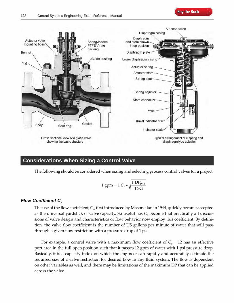
128 Control Systems Engineering Exam Reference Manual
Considerations When Sizing a Control Valve
The following should be considered when sizing and selecting process control valves for a project.
1 11
1 gpm
SG
psig= Cv iDP
Flow Coefficient Cv
The use of the flow coefficient, Cv, first introduced by Masoneilan in 1944, quickly became accepted as the universal yardstick of valve capacity. So useful has Cv become that practically all discus-sions of valve design and characteristics or flow behavior now employ this coefficient. By defini-tion, the valve flow coefficient is the number of US gallons per minute of water that will pass through a given flow restriction with a pressure drop of 1 psi.
For example, a control valve with a maximum flow coefficient of Cv = 12 has an effective port area in the full open position such that it passes 12 gpm of water with 1 psi pressure drop. Basically, it is a capacity index on which the engineer can rapidly and accurately estimate the required size of a valve restriction for desired flow in any fluid system. The flow is dependent on other variables as well, and there may be limitations of the maximum DP that can be applied across the valve.
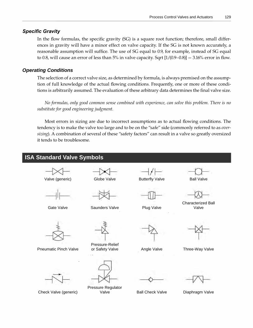
129Process Control Valves and Actuators
Specific GravityIn the flow formulas, the specific gravity (SG) is a square root function; therefore, small differ-ences in gravity will have a minor effect on valve capacity. If the SG is not known accurately, a reasonable assumption will suffice. The use of SG equal to 0.9, for example, instead of SG equal to 0.8, will cause an error of less than 5% in valve capacity. Sqrt [1/(0.9–0.8)] = 3.16% error in flow.
Operating ConditionsThe selection of a correct valve size, as determined by formula, is always premised on the assump-tion of full knowledge of the actual flowing conditions. Frequently, one or more of these condi-tions is arbitrarily assumed. The evaluation of these arbitrary data determines the final valve size.
No formulas, only good common sense combined with experience, can solve this problem. There is no substitute for good engineering judgment.
Most errors in sizing are due to incorrect assumptions as to actual flowing conditions. The tendency is to make the valve too large and to be on the “safe” side (commonly referred to as over-sizing). A combination of several of these “safety factors” can result in a valve so greatly oversized it tends to be troublesome.
ISA Standard Valve Symbols
Valve (generic) Globe Valve Butterfly Valve Ball Valve
Gate Valve Saunders Valve Plug ValveCharacterized Ball
Valve
Pneumatic Pinch ValvePressure-Relief or Safety Valve Angle Valve Three-Way Valve
Check Valve (generic)Pressure Regulator
Valve Ball Check Valve Diaphragm Valve
161
14 Pressure-Relief Valves and Rupture Disks
Pressure-Relief Valves and Pressure Safety Valves
Gases and steams can be compressed. When gas reaches the disk in a valve, it compresses and builds up pressure before escaping through the valve. This compression can cause system pres-sure to build up rapidly. A liquid-type relief valve does not open fast enough to relieve gas or steam pressure. A gas system requires a valve that can open completely under excess pressure, or a pressure safety valve.
Pressure safety valve (PSV) and pressure-relief valve (PRV) are commonly used terms to identify pressure-relief devices on a vessel. These terms are often used interchangeably; depending on the project or company standards, pressure-relief devices may be identified as safety valves or as relief valves, or sometimes even as safety relief valves.
Although used freely and interchangeably, these terms differ:
• Pressure-relief valve is the term used to describe a relief device on a liquid-filled vessel. Forsuch a valve, the opening is proportional to the increase in the vessel pressure. Therefore,the opening of the valve is not sudden but gradual, if the pressure is increased gradually.
Note: Do not throttle pressure-relief valves.
• Pressure safety valve is the term used to describe a relief device on a compressible fluid orgas-filled vessel. For this type of valve, the opening is sudden. When the set pressure of thevalve is reached, the valve opens almost fully.
A PRV should not be used to control the pressure out of a pump. The PRV will chatter, and the hammering action caused by the pulsations will quickly destroy the valve. A proportional control valve should be used for this application. Contact the manufacturer for more information about this application.
162 Control Systems Engineering Exam Reference Manual
Environmental Protection Agency Regulations
Many environmental protection agencies worldwide have been tightening regulations on hazard-ous material emissions. In the United States, for example, the Environmental Protection Agency (EPA) has been issuing new and stricter regulations for several types of industries, ranging from food and beverage to nuclear power plants. There are regulations for refineries, with specific sec-tions for each type of plant unit, such as fluid catalytic cracking units, catalytic reforming units, utilities, storage, and water treatment. The requirements for refineries and other types of indus-tries are similar, with the main difference being the tolerated amounts for each type of pollutant released. The more stringent rules established by the new EPA regulations issued in September 2015 and by other environmental agencies can be generalized with three simple requirements:
1. Provide indication and location where a pressure-relief device (PRD) event occurs throughelectronic monitoring.
2. Measure the time and duration of the PRD event for recording and reporting of emissionsreleases from:
A. Protected vessel
B. Rupture disc
C. Relief valve
D. Bypass valve
3. Notify the operator of the event so corrective action can occur.
Also, the EPA expects “flare operation at all times during the process of gas being sent to the flare,” so quick identification of a PRD release is not optional. In general, newer and more strin-gent rules apply not only to normal operation, but also to start-up/shutdown periods, where there have historically been more leniencies. These start-up/shutdown periods are often when process upsets are most likely to occur, so compliance with these new regulations can be demanding.
Plants must comply with environmental regulations by law. Failing to do so can cause serious damage to the environment and personnel. It can also cause explosions and serious damage to plant equipment. In addition, lack of compliance can result in expensive fines, production dis-ruptions, and bad publicity. But there is another compelling reason to monitor and curb fugitive emissions: leakages caused by PRD malfunctions can waste large amounts of valuable products, along with the energy required to produce such products.
Regulation DetailsEvery national and international government has its own rules to control and monitor emissions of pollutants. In the United States, the Clean Air Act (CAA) is the key federal law regulating air emissions from stationary and mobile sources. Among other things, this law authorizes the EPA to establish national ambient air quality standards to protect public health and public welfare by regulating emissions of hazardous air pollutants. CAA Section 111(b) requires the EPA to set and
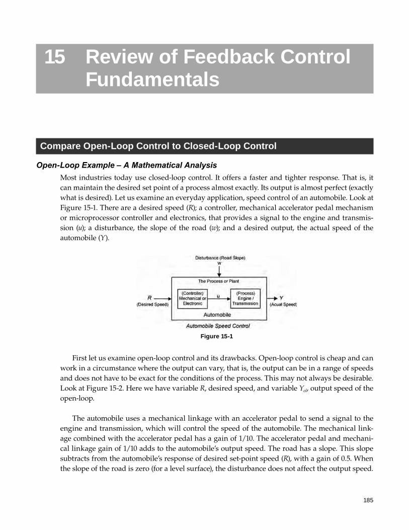
185
15 Review of Feedback Control Fundamentals
Compare Open-Loop Control to Closed-Loop Control
Open-Loop Example – A Mathematical AnalysisMost industries today use closed-loop control. It offers a faster and tighter response. That is, it can maintain the desired set point of a process almost exactly. Its output is almost perfect (exactly what is desired). Let us examine an everyday application, speed control of an automobile. Look at Figure 15-1. There are a desired speed (R); a controller, mechanical accelerator pedal mechanism or microprocessor controller and electronics, that provides a signal to the engine and transmis-sion (u); a disturbance, the slope of the road (w); and a desired output, the actual speed of the automobile (Y).
First let us examine open-loop control and its drawbacks. Open-loop control is cheap and can work in a circumstance where the output can vary, that is, the output can be in a range of speeds and does not have to be exact for the conditions of the process. This may not always be desirable. Look at Figure 15-2. Here we have variable R, desired speed, and variable Yol, output speed of the open-loop.
The automobile uses a mechanical linkage with an accelerator pedal to send a signal to the engine and transmission, which will control the speed of the automobile. The mechanical link-age combined with the accelerator pedal has a gain of 1/10. The accelerator pedal and mechani-cal linkage gain of 1/10 adds to the automobile’s output speed. The road has a slope. This slope subtracts from the automobile’s response of desired set-point speed (R), with a gain of 0.5. When the slope of the road is zero (for a level surface), the disturbance does not affect the output speed.
Figure 15-1
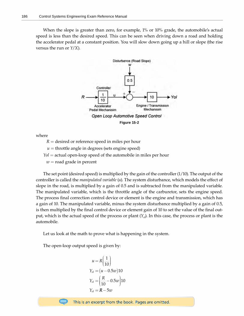
186 Control Systems Engineering Exam Reference Manual
When the slope is greater than zero, for example, 1% or 10% grade, the automobile’s actual speed is less than the desired speed. This can be seen when driving down a road and holding the accelerator pedal at a constant position. You will slow down going up a hill or slope (the rise versus the run or Y/X).
whereR = desired or reference speed in miles per hour
u = throttle angle in degrees (sets engine speed)
Yol = actual open-loop speed of the automobile in miles per hour
w = road grade in percent
The set point (desired speed) is multiplied by the gain of the controller (1/10). The output of the controller is called the manipulated variable (u). The system disturbance, which models the effect of slope in the road, is multiplied by a gain of 0.5 and is subtracted from the manipulated variable. The manipulated variable, which is the throttle angle of the carburetor, sets the engine speed. The process final correction control device or element is the engine and transmission, which has a gain of 10. The manipulated variable, minus the system disturbance multiplied by a gain of 0.5, is then multiplied by the final control device or element gain of 10 to set the value of the final out-put, which is the actual speed of the process or plant (Yol). In this case, the process or plant is the automobile.
Let us look at the math to prove what is happening in the system.
The open-loop output speed is given by:
u R
Y u w
YR
w
Y
ol
ol
ol
=
= −( )
= −
=
110
0 5 10
100 5 10
.
.
RR w− 5
Figure 15-2
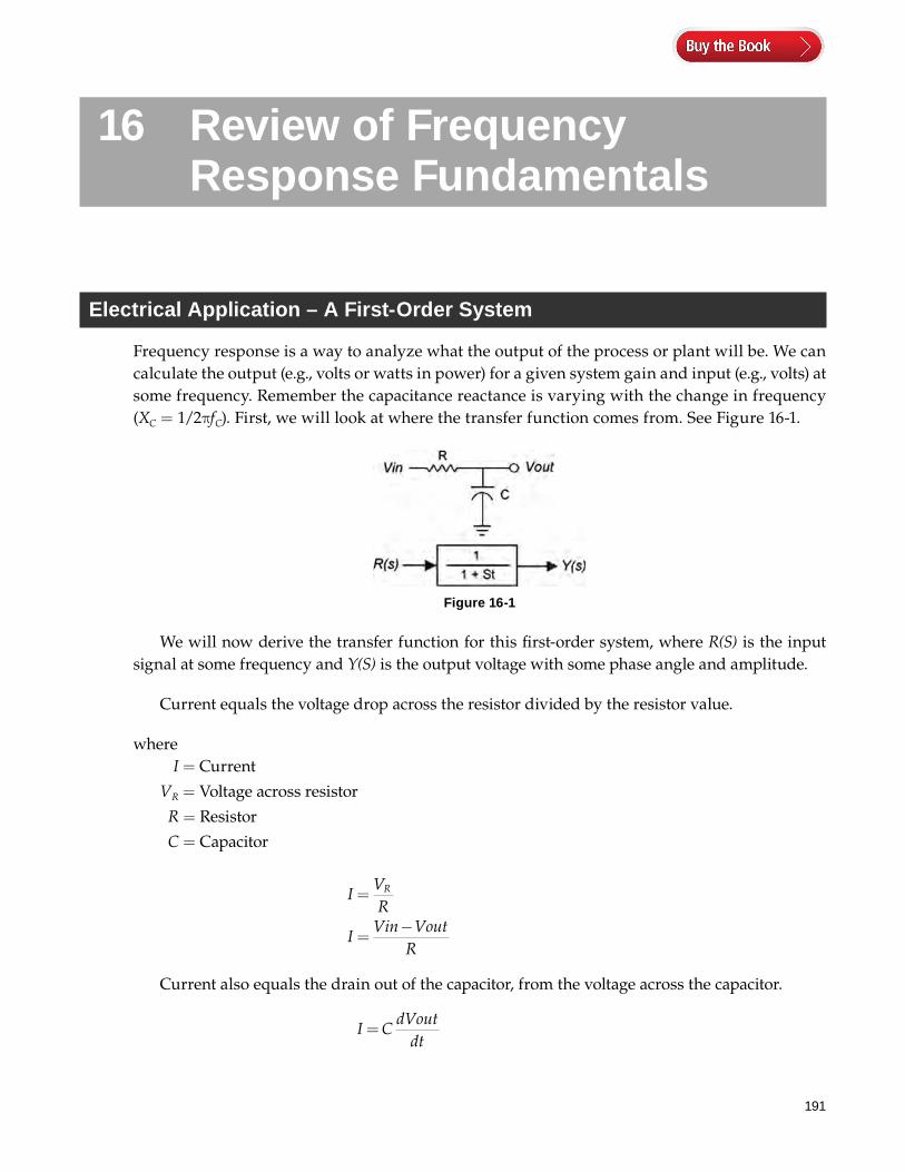
191
16 Review of Frequency Response Fundamentals
Electrical Application – A First-Order System
Frequency response is a way to analyze what the output of the process or plant will be. We can calculate the output (e.g., volts or watts in power) for a given system gain and input (e.g., volts) at some frequency. Remember the capacitance reactance is varying with the change in frequency (XC = 1/2πfC). First, we will look at where the transfer function comes from. See Figure 16-1.
We will now derive the transfer function for this first-order system, where R(S) is the input signal at some frequency and Y(S) is the output voltage with some phase angle and amplitude.
Current equals the voltage drop across the resistor divided by the resistor value.
whereI = Current
VR = Voltage across resistor
R = Resistor
C = Capacitor
IVR
IVin Vout
R
R=
=−
Current also equals the drain out of the capacitor, from the voltage across the capacitor.
I CdVout
dt=
Figure 16-1
192 Control Systems Engineering Exam Reference Manual
Substitute voltage drop divided by resistance for amps (I) and set the two equations equal to each other.
Vin VoutR
CdVout
dt−
=
Vin Vout RCdVout
dt− =
Sddt
=
Vin Vout RCS Vout− = ( )
Vin Vout RCS Vout= + ( )
Vin RCS Vout= +( )1
VinRCS
Vout
RCSVoutVin
t RC
11
1
+=
+=
=
The transfer function is equal to the gain of the system.
11+
=St
VoutVin
Use the transfer function to calculate the voltage out of the system.
VinSt
Vout1
1+
=
We have derived the transfer function for this first-order system. We can now plug in an input voltage and an angular frequency and calculate the attenuation of the output signal and the phase angle of the output signal.
Bode Plot of First-Order System
Make a Bode plot for a circuit with the following components.
resistor = 1000 Ω
capacitor = 2.65 µF
199
17 Control Theory and Controller Tuning
The process control industry covers a wide variety of applications: petrochemical, pharmaceuti-cal, power generation, water treatment, pulp and paper, food processing, material handling, and even commercial applications.
Process control in a plant can includes discrete logic, such as relay logic or a programmable logic controller (PLC); analog control, such as single-loop control or a distributed control system (DCS); pneumatic systems; hydraulic systems; and electrical systems. The control systems engi-neer must be versatile and understand a broad range of control subjects as applied to controller applications, configuration, and tuning, as well as analysis and understanding of loop gain and stability.
This section will review the foundations of process control theory and its applications. Some of this material may be on the CSE exam. I have tried to keep the studies to a minimum and reduce the math for the problems to a form in which you can just plug in the values and get the answer you need for the exam.
We will cover degrees of freedom, process loop gain and applications, filtering of noise in pro-cess variable (PV) signals, open- and closed-loop tuning, damping of the system, time constants, overshoot of process set points, and checking for stability of a system transfer function.
Degrees of Freedom in Process Control Systems
In an unconstrained system, the number of independent variables required to completely specify the state of the system at a given moment must be defined. If the system has constraints, that is, kinematic or geometric relations between the variables, each such independent relation reduces by one the number of degrees of freedom (DOF) of the system.
process variables – (equations + constraints) = DOFDOF = minimum number of process controllers required
200 Control Systems Engineering Exam Reference Manual
Example 1: An Airplane
VariablesAltitude 1Latitude 1Longitude 1
3Minus Constraints 0Minus Equations 0DOF = 3
DOF = 3 − (0 + 0) = 3Three controllers are needed, one for each variable.
Example 2: A Train
VariablesAltitude 1Latitude 1Longitude 1
3Minus Constraints Altitude 1Latitude 1Minus Equations 0DOF = 1
DOF = 3 − (2 + 0) = 1One controller is needed; one for longitude only.
Example 3: A Hot Water Heat Exchanger
VariablesWS (flow rate of steam) 1WCW (flow rate of cold water) 1WHW (flow rate of hot water) 1Q (quantity of steam in cubic feet) 1PS (supply pressure of steam) 1TCW (temperature of cold water) 1THW (temperature of hot water) 1
7Minus Constraints or ConstantsQ (quantity of steam) 1PS (supply pressure of steam) 1TCW (temperature of cold water) 1
3

231
18 Communications and Control Networks
Overview of Corporate and Plant Networks
On the CSE exam, there may be a few questions on fieldbus, intelligent devices, and networks. We will briefly review the highlights of these subjects. For more information on fieldbus, contact your local distributor.
Fieldbus is a digital, two-way, multidrop communication link among intelligent control devices that replaces the 4–20 mA analog standard devices. The key to fieldbus is that the device is digital, not analog. There are numerous protocols on the international market. Foundation Fieldbus, PROFIBUS, AS/i, ControlNet, DeviceNet, Modbus, and HART are the most popular in the process industry.
The most popular types of fieldbus typically use EIA-485 protocol with token passing and 31.25 kbps on a single twisted pair wire that can be run up to 1900 m. They can have 32 segments and 1024 intelligent devices per network.
The connected intelligent devices are not calibrated; the data is scaled in software. Intelligent devices may deliver from 1 up to 12 or more data variables of information from one instrument. The data is delivered in data packets to the intelligent control device or master. With Foundation

232 Control Systems Engineering Exam Reference Manual
Fieldbus, any intelligent device can be the controller. More than likely, the valve may be selected as the intelligent controller that will be responsible for the PID calculation for its control loop.
Intelligent devices must be configured when first installed. This is done through Electronic Device Description Language or Field Device Tool. Most of the intelligent devices are plug-and-play. PROFIBUS devices can even be changed out without reconfiguring the device once it is initially configured. The configuration data is stored by the master controller and is then auto-matically downloaded to the new device on connection to the network.
Networks can be connected by wire or fiber-optic cable, or can be wireless. There are three major categories of networks: LAN (local area network), WAN (wide area network), and MAN (metro-politan area network). The LAN is typically limited to 100 m (or 330 ft per segment) and 1024 nodes.
Industrial instruments typically communicate through a version of one of the three commu-nication network protocols:
1. In a fieldbus network, they use one of the previously mentioned networks.
2. In a serial network, they use EIA/RS-232, EIA/RS-485, or EIA/RS-488.
3. In an Ethernet network, they use Ethernet/IEEE 802.3, Token Ring/IEEE 802.5, and the fiberdistributed data interface (FDDI). A fiber backbone for the control system usually usesIEEE 802.1Q. This is a 1-gigabit Ethernet network.
Three typical Ethernet networks. Ethernet protocols.
If the device communicates through Ethernet protocol, it typically has a media access control (MAC) address. Like a social security number, this number is unique to each device. For a device on one network to talk to a device on another network using a different protocol, a protocol con-verter or gateway is needed.
Open System Interconnect and TCP/IP Network Layer Model
Seven Layers of Networking in the Open System Interconnect ModelThe network layers in the Open System Interconnect (OSI) model enable us to break down func-tional steps in communication by program protocols. You can think of protocols as the different steps in an assembly line. Computers communicate with each other through encapsulating or
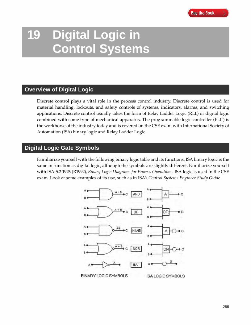
255
19 Digital Logic in Control Systems
Overview of Digital Logic
Discrete control plays a vital role in the process control industry. Discrete control is used for material handling, lockouts, and safety controls of systems, indicators, alarms, and switching applications. Discrete control usually takes the form of Relay Ladder Logic (RLL) or digital logic combined with some type of mechanical apparatus. The programmable logic controller (PLC) is the workhorse of the industry today and is covered on the CSE exam with International Society of Automation (ISA) binary logic and Relay Ladder Logic.
Digital Logic Gate Symbols
Familiarize yourself with the following binary logic table and its functions. ISA binary logic is the same in function as digital logic, although the symbols are slightly different. Familiarize yourself with ISA-5.2-1976 (R1992), Binary Logic Diagrams for Process Operations. ISA logic is used in the CSE exam. Look at some examples of its use, such as in ISA’s Control Systems Engineer Study Guide.
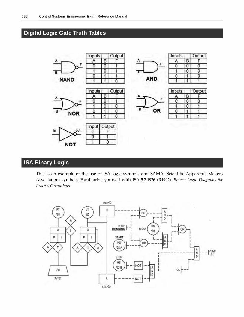
256 Control Systems Engineering Exam Reference Manual
Digital Logic Gate Truth Tables
ISA Binary Logic
This is an example of the use of ISA logic symbols and SAMA (Scientific Apparatus Makers Association) symbols. Familiarize yourself with ISA-5.2-1976 (R1992), Binary Logic Diagrams for Process Operations.

265
20 Motor Control and Logic Functions
The figures below show how a motor control center (MCC) is implemented in a plant electrical system.
Plant Electrical System
Motor Control Center (MCC)

266 Control Systems Engineering Exam Reference Manual
Typical MCC Design
This a typical MCC found in most plants. It is a modular and expandable unit. The smaller squares are the motor starter compartments (see right unit).
The compartments are called buck-ets, and the wiring can be quickly dis-connected and the bucket removed and replaced for fast repair and turn-around during shutdowns and design expansions.
The buckets typically slide in or plug into a vertical busbar with spring-clamped contacts, this is called stab-in design. But some buckets are wired to the busbar. They take up differ-ent vertical dimensions based on the motor starter size. These dimensions are called space factors.
The MCC can come with 42 circuit panelboards, small power transformers, variable frequency drives (VFDs), heater and lighting contactors, breakers, and switches. Spare units and blank cov-ers (called spaces) are available for future expansion and can also be installed.
Most MCCs today are equipped with a programmable logic controller (PLC) or human-machine interface (HMI) and a communications network for controlling the MCC remotely as well as power usage monitoring. The networks are typically DeviceNet or Ethernet or an older technology such as Modbus RS-485 serial networks.
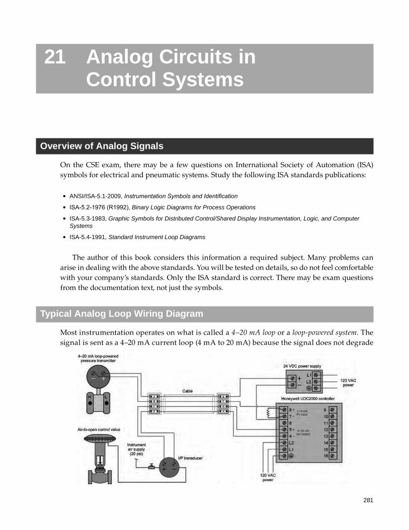
281
21 Analog Circuits in Control Systems
Overview of Analog Signals
On the CSE exam, there may be a few questions on International Society of Automation (ISA) symbols for electrical and pneumatic systems. Study the following ISA standards publications:
The author of this book considers this information a required subject. Many problems can arise in dealing with the above standards. You will be tested on details, so do not feel comfortable with your company’s standards. Only the ISA standard is correct. There may be exam questions from the documentation text, not just the symbols.
Typical Analog Loop Wiring Diagram
Most instrumentation operates on what is called a 4–20 mA loop or a loop-powered system. The signal is sent as a 4–20 mA current loop (4 mA to 20 mA) because the signal does not degrade
• ANSI/ISA-5.1-2009, Instrumentation Symbols and Identification
• ISA-5.2-1976 (R1992), Binary Logic Diagrams for Process Operations
• ISA-5.3-1983, Graphic Symbols for Distributed Control/Shared Display Instrumentation, Logic, and ComputerSystems
• ISA-5.4-1991, Standard Instrument Loop Diagrams
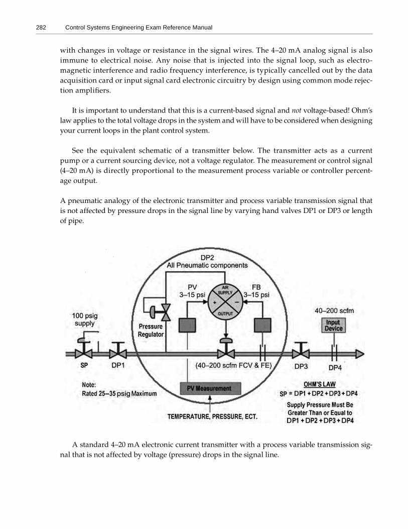
282 Control Systems Engineering Exam Reference Manual
with changes in voltage or resistance in the signal wires. The 4–20 mA analog signal is also immune to electrical noise. Any noise that is injected into the signal loop, such as electro-magnetic interference and radio frequency interference, is typically cancelled out by the data acquisition card or input signal card electronic circuitry by design using common mode rejec-tion amplifiers.
It is important to understand that this is a current-based signal and not voltage-based! Ohm’s law applies to the total voltage drops in the system and will have to be considered when designing your current loops in the plant control system.
See the equivalent schematic of a transmitter below. The transmitter acts as a current pump or a current sourcing device, not a voltage regulator. The measurement or control signal (4–20 mA) is directly proportional to the measurement process variable or controller percent-age output.
A pneumatic analogy of the electronic transmitter and process variable transmission signal that is not affected by pressure drops in the signal line by varying hand valves DP1 or DP3 or length of pipe.
A standard 4–20 mA electronic current transmitter with a process variable transmission sig-nal that is not affected by voltage (pressure) drops in the signal line.
295
22 Overview of Motion Controller Applications
Motion Control Systems
The basic architecture of a motion control system contains:
• A motion controller to move something to a desired position or set and maintain the veloc-ity of a system component or fluid. Motion controllers typically use closed-loop feedback,but not always.
• A drive or amplifier to transform the control signal from the motion controller into a higherpower electrical current or voltage that is presented to the actuator.
• An actuator such as a hydraulic pump, air cylinder, linear actuator, or electric motor foroutput of motion.
• One or more feedback sensors, such as optical encoders, resolvers, or Hall effect devices, toreturn the position or velocity of the actuator to the motion controller in order to close theposition or velocity control loops.
• Mechanical components to transform the motion of the actuator into the desiredmotion, including gears, shafting, ball screws, belts, linkages, and linear and rotationalbearings.
Common control functions include:
• Velocity control.
• Position (point-to-point) control: There are several methods for computing a motion trajec-tory. These are often based on the velocity profiles of a move, such as a triangular profile,trapezoidal profile, or an S-curve profile.
• Pressure or force control.
• Electronic gearing (or cam profiling).
296 Control Systems Engineering Exam Reference Manual
Stepper Motors
A stepper motor is a brushless, synchronous electric motor that converts digital pulses into mechanical shaft rotation.
Every revolution of the stepper motor is divided into a discrete number of steps, in many cases 200 steps, and the motor must be sent a separate pulse for each step. The stepper motor can only take one step at a time, and each step is the same size. Because each pulse causes the motor to rotate a precise angle, typically 1.8°, the motor’s position can be controlled without any feedback mechanism. As the digital pulses increase in frequency, the step movement changes into con-tinuous rotation, with the speed of rotation directly proportional to the frequency of the pulses. Stepper motors are used every day in both industrial and commercial applications because of their low cost, high reliability, high torque at low speeds, and simple, rugged construction that operates in almost any environment.
Closed-Loop Stepper MotorModern motion controllers can include the ability to run stepper motors with encoder feedback, resulting in true closed-loop motion control. This mode of motor control is similar to standard three-phase brushless servo motor control, where the three phases are offset 120 electrical degrees. With steppers, the motor has two phases offset by 90 electrical degrees. The benefits of closed-loop control with stepper motors include greatly improved velocity smoothness and reduced power consumption (compared to open-loop steppers) and much higher torque at low velocity (com-pared with traditional three-phase brushless servomotors).
Stepper Motor Advantages1. The rotation angle of the motor is proportional to the input pulse.
2. The motor has full torque at standstill (if the windings are energized).
3. Precise positioning and repeatability of movement because good stepper motors have anaccuracy of 3%–5% of a step and this error is noncumulative from one step to the next.
4. Excellent response to starting/stopping/reversing of the motor.
5. Very reliable because there are no contact brushes in the motor. Therefore, the life of thestepper motor is simply dependent on the life of the bearing.
6. The stepper motor’s response to digital input pulses provides open-loop control, makingthe motor simpler and less costly to control.
7. It is possible to achieve very low speed synchronous rotation with a load that is directlycoupled to the shaft.
8. A wide range of rotational speeds can be realized as the speed is proportional to the fre-quency of the input pulses.
9. Linear motion control with lead screw or worm gears.
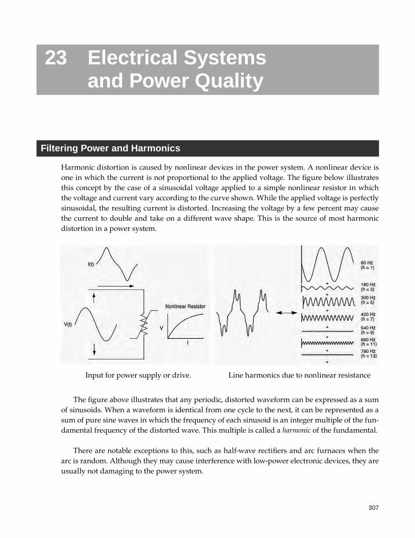
307
23 Electrical Systems and Power Quality
Filtering Power and Harmonics
Harmonic distortion is caused by nonlinear devices in the power system. A nonlinear device is one in which the current is not proportional to the applied voltage. The figure below illustrates this concept by the case of a sinusoidal voltage applied to a simple nonlinear resistor in which the voltage and current vary according to the curve shown. While the applied voltage is perfectly sinusoidal, the resulting current is distorted. Increasing the voltage by a few percent may cause the current to double and take on a different wave shape. This is the source of most harmonic distortion in a power system.
Input for power supply or drive. Line harmonics due to nonlinear resistance
The figure above illustrates that any periodic, distorted waveform can be expressed as a sum of sinusoids. When a waveform is identical from one cycle to the next, it can be represented as a sum of pure sine waves in which the frequency of each sinusoid is an integer multiple of the fun-damental frequency of the distorted wave. This multiple is called a harmonic of the fundamental.
There are notable exceptions to this, such as half-wave rectifiers and arc furnaces when the arc is random. Although they may cause interference with low-power electronic devices, they are usually not damaging to the power system.
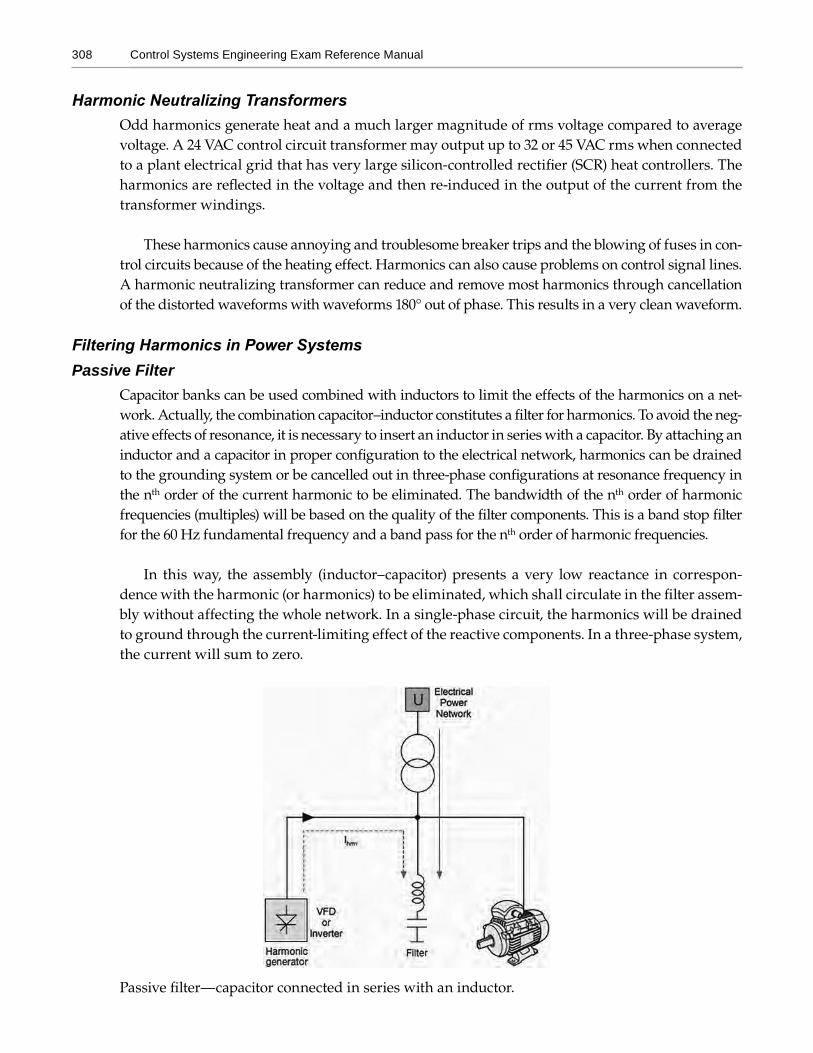
308 Control Systems Engineering Exam Reference Manual
Harmonic Neutralizing TransformersOdd harmonics generate heat and a much larger magnitude of rms voltage compared to average voltage. A 24 VAC control circuit transformer may output up to 32 or 45 VAC rms when connected to a plant electrical grid that has very large silicon-controlled rectifier (SCR) heat controllers. The harmonics are reflected in the voltage and then re-induced in the output of the current from the transformer windings.
These harmonics cause annoying and troublesome breaker trips and the blowing of fuses in con-trol circuits because of the heating effect. Harmonics can also cause problems on control signal lines. A harmonic neutralizing transformer can reduce and remove most harmonics through cancellation of the distorted waveforms with waveforms 180° out of phase. This results in a very clean waveform.
Filtering Harmonics in Power SystemsPassive Filter
Capacitor banks can be used combined with inductors to limit the effects of the harmonics on a net-work. Actually, the combination capacitor–inductor constitutes a filter for harmonics. To avoid the neg-ative effects of resonance, it is necessary to insert an inductor in series with a capacitor. By attaching an inductor and a capacitor in proper configuration to the electrical network, harmonics can be drained to the grounding system or be cancelled out in three-phase configurations at resonance frequency in the nth order of the current harmonic to be eliminated. The bandwidth of the nth order of harmonic frequencies (multiples) will be based on the quality of the filter components. This is a band stop filter for the 60 Hz fundamental frequency and a band pass for the nth order of harmonic frequencies.
In this way, the assembly (inductor–capacitor) presents a very low reactance in correspon-dence with the harmonic (or harmonics) to be eliminated, which shall circulate in the filter assem-bly without affecting the whole network. In a single-phase circuit, the harmonics will be drained to ground through the current-limiting effect of the reactive components. In a three-phase system, the current will sum to zero.
Passive filter—capacitor connected in series with an inductor.

313
24 Emergency Standby Systems
NEC Article 700 – Emergency SystemsThe requirements of Article 700 apply only to the wiring methods for “emergency systems” that are essential for safety to human life and are required by federal, state, or municipal governments or other agencies having jurisdiction. When normal power is lost, emergency systems shall be able to supply standby power in 10 s or less.
NEC Article 701 – Legally Required Standby SystemsLegally required standby systems provide electric power to aid in firefighting, rescue operations, control of health hazards, and similar operations. When normal power is lost, legally required systems shall be able to supply standby power in 60 s or less, instead of the 10 s or less required of emergency systems.
NEC Article 702 – Optional Standby SystemsOptional standby systems are intended to protect public or private facilities or property where life safety does not depend on the performance of the system. These systems are typically installed to provide an alternate source of electric power for such facilities as industrial and commercial buildings, farms, and residences, and to serve loads that, when stopped during any power outage, could cause discomfort, serious interruption of the process, or damage to the product or process. Optional standby systems are intended to supply on-site generated power to selected loads either automatically or manually.
Uninterruptible Power Supply
An uninterruptible power supply (UPS), also called uninterruptible power source or battery/flywheel backup, is an electrical apparatus that provides emergency power to a load when the input power source, typically the main power, fails. A UPS differs from an auxiliary or emergency power system or standby generator in that it will provide nearly instantaneous protection from input power interruptions by supplying energy stored in batteries, supercapacitors, or flywheels. The on-battery runtime of most UPSs is relatively short, only a few minutes to a few hours (maybe up
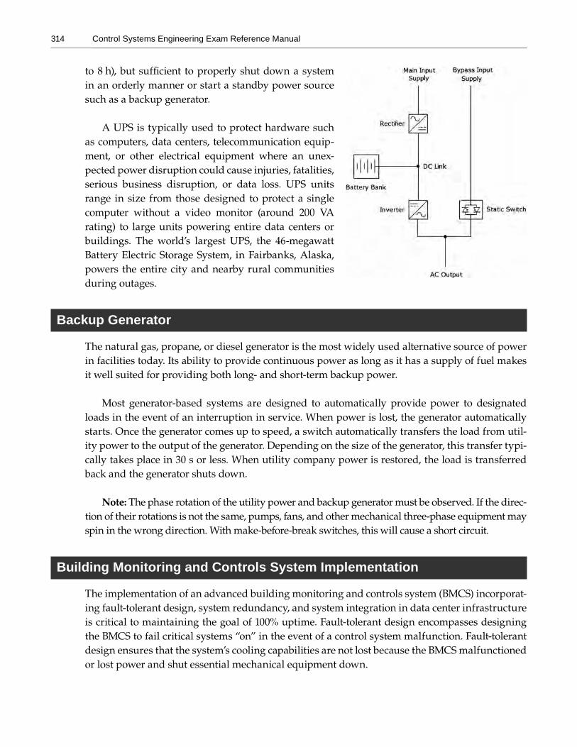
314 Control Systems Engineering Exam Reference Manual
to 8 h), but sufficient to properly shut down a system in an orderly manner or start a standby power source such as a backup generator.
A UPS is typically used to protect hardware such as computers, data centers, telecommunication equip-ment, or other electrical equipment where an unex-pected power disruption could cause injuries, fatalities, serious business disruption, or data loss. UPS units range in size from those designed to protect a single computer without a video monitor (around 200 VA rating) to large units powering entire data centers or buildings. The world’s largest UPS, the 46-megawatt Battery Electric Storage System, in Fairbanks, Alaska, powers the entire city and nearby rural communities during outages.
Backup Generator
The natural gas, propane, or diesel generator is the most widely used alternative source of power in facilities today. Its ability to provide continuous power as long as it has a supply of fuel makes it well suited for providing both long- and short-term backup power.
Most generator-based systems are designed to automatically provide power to designated loads in the event of an interruption in service. When power is lost, the generator automatically starts. Once the generator comes up to speed, a switch automatically transfers the load from util-ity power to the output of the generator. Depending on the size of the generator, this transfer typi-cally takes place in 30 s or less. When utility company power is restored, the load is transferred back and the generator shuts down.
Note: The phase rotation of the utility power and backup generator must be observed. If the direc-tion of their rotations is not the same, pumps, fans, and other mechanical three-phase equipment may spin in the wrong direction. With make-before-break switches, this will cause a short circuit.
Building Monitoring and Controls System Implementation
The implementation of an advanced building monitoring and controls system (BMCS) incorporat-ing fault-tolerant design, system redundancy, and system integration in data center infrastructure is critical to maintaining the goal of 100% uptime. Fault-tolerant design encompasses designing the BMCS to fail critical systems “on” in the event of a control system malfunction. Fault-tolerant design ensures that the system’s cooling capabilities are not lost because the BMCS malfunctioned or lost power and shut essential mechanical equipment down.
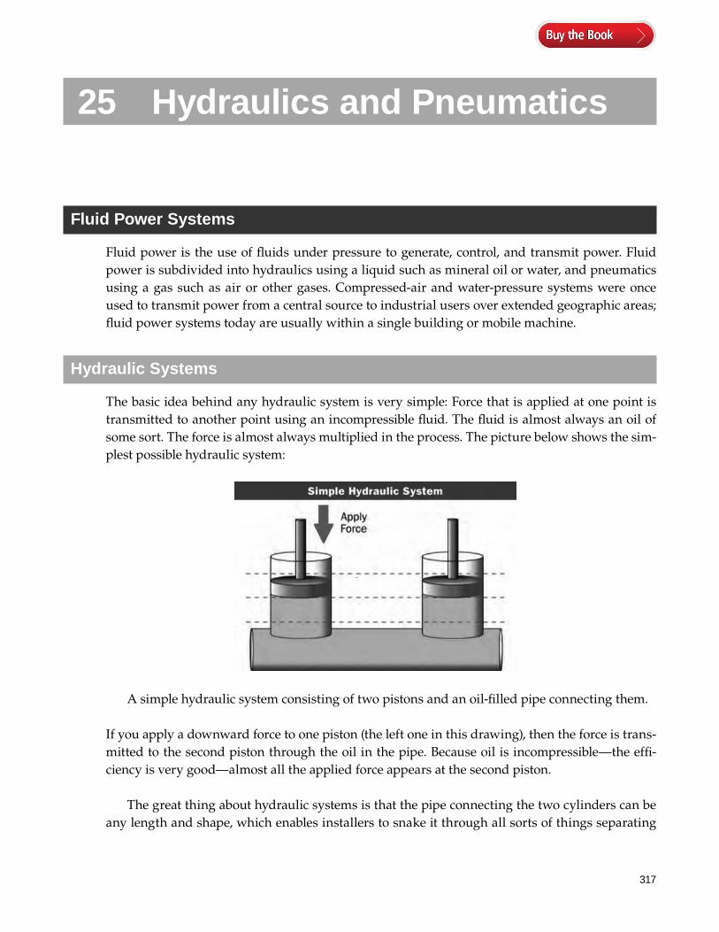
317
25 Hydraulics and Pneumatics
Fluid Power Systems
Fluid power is the use of fluids under pressure to generate, control, and transmit power. Fluid power is subdivided into hydraulics using a liquid such as mineral oil or water, and pneumatics using a gas such as air or other gases. Compressed-air and water-pressure systems were once used to transmit power from a central source to industrial users over extended geographic areas; fluid power systems today are usually within a single building or mobile machine.
Hydraulic Systems
The basic idea behind any hydraulic system is very simple: Force that is applied at one point is transmitted to another point using an incompressible fluid. The fluid is almost always an oil of some sort. The force is almost always multiplied in the process. The picture below shows the sim-plest possible hydraulic system:
A simple hydraulic system consisting of two pistons and an oil-filled pipe connecting them.
If you apply a downward force to one piston (the left one in this drawing), then the force is trans-mitted to the second piston through the oil in the pipe. Because oil is incompressible—the effi-ciency is very good—almost all the applied force appears at the second piston.
The great thing about hydraulic systems is that the pipe connecting the two cylinders can be any length and shape, which enables installers to snake it through all sorts of things separating
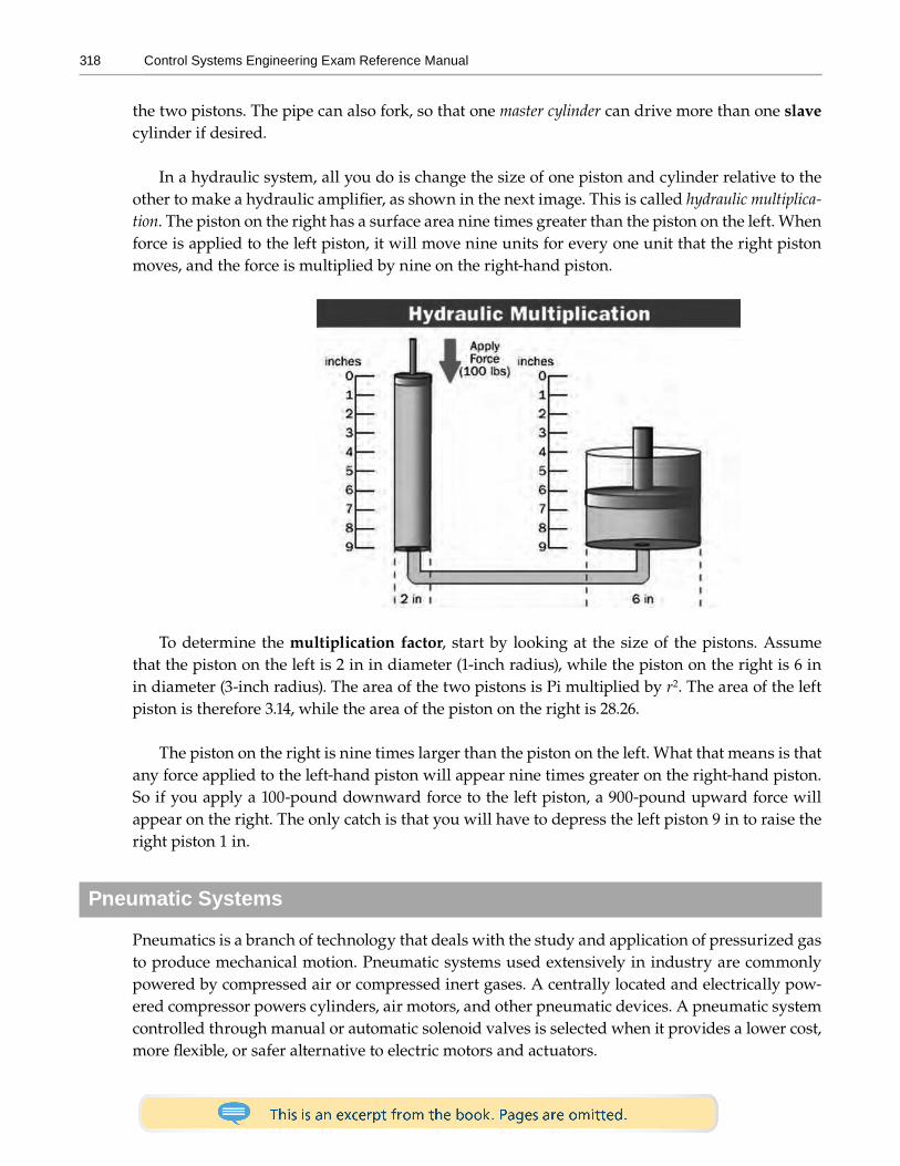
318 Control Systems Engineering Exam Reference Manual
the two pistons. The pipe can also fork, so that one master cylinder can drive more than one slave cylinder if desired.
In a hydraulic system, all you do is change the size of one piston and cylinder relative to the other to make a hydraulic amplifier, as shown in the next image. This is called hydraulic multiplica-tion. The piston on the right has a surface area nine times greater than the piston on the left. When force is applied to the left piston, it will move nine units for every one unit that the right piston moves, and the force is multiplied by nine on the right-hand piston.
To determine the multiplication factor, start by looking at the size of the pistons. Assume that the piston on the left is 2 in in diameter (1-inch radius), while the piston on the right is 6 in in diameter (3-inch radius). The area of the two pistons is Pi multiplied by r2. The area of the left piston is therefore 3.14, while the area of the piston on the right is 28.26.
The piston on the right is nine times larger than the piston on the left. What that means is that any force applied to the left-hand piston will appear nine times greater on the right-hand piston. So if you apply a 100-pound downward force to the left piston, a 900-pound upward force will appear on the right. The only catch is that you will have to depress the left piston 9 in to raise the right piston 1 in.
Pneumatic Systems
Pneumatics is a branch of technology that deals with the study and application of pressurized gas to produce mechanical motion. Pneumatic systems used extensively in industry are commonly powered by compressed air or compressed inert gases. A centrally located and electrically pow-ered compressor powers cylinders, air motors, and other pneumatic devices. A pneumatic system controlled through manual or automatic solenoid valves is selected when it provides a lower cost, more flexible, or safer alternative to electric motors and actuators.
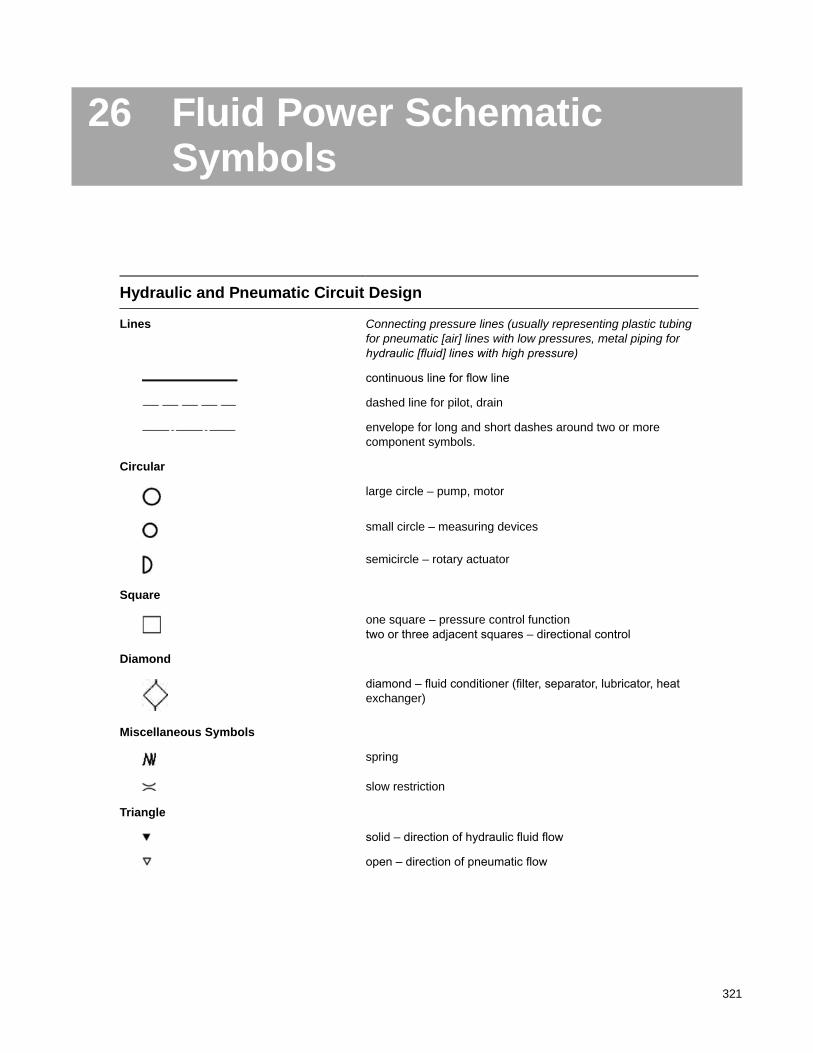
321
26 Fluid Power Schematic Symbols
Hydraulic and Pneumatic Circuit Design
Lines Connecting pressure lines (usually representing plastic tubing for pneumatic [air] lines with low pressures, metal piping for hydraulic [fluid] lines with high pressure)
continuous line for flow line
dashed line for pilot, drain
envelope for long and short dashes around two or more component symbols.
Circular
large circle – pump, motor
small circle – measuring devices
semicircle – rotary actuator
Square
one square – pressure control function two or three adjacent squares – directional control
Diamond
diamond – fluid conditioner (filter, separator, lubricator, heat exchanger)
Miscellaneous Symbols
spring
slow restriction
Triangle
solid – direction of hydraulic fluid flow
open – direction of pneumatic flow
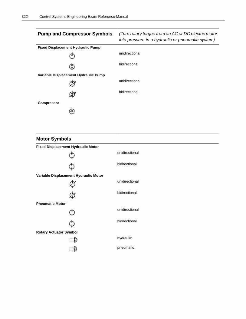
322 Control Systems Engineering Exam Reference Manual
Motor SymbolsFixed Displacement Hydraulic Motor
unidirectional
bidirectional
Variable Displacement Hydraulic Motorunidirectional
bidirectional
Pneumatic Motorunidirectional
bidirectional
Rotary Actuator Symbolhydraulic
pneumatic
Pump and Compressor Symbols (Turn rotary torque from an AC or DC electric motor into pressure in a hydraulic or pneumatic system)
Fixed Displacement Hydraulic Pumpunidirectional
bidirectional
Variable Displacement Hydraulic Pumpunidirectional
bidirectional
Compressor
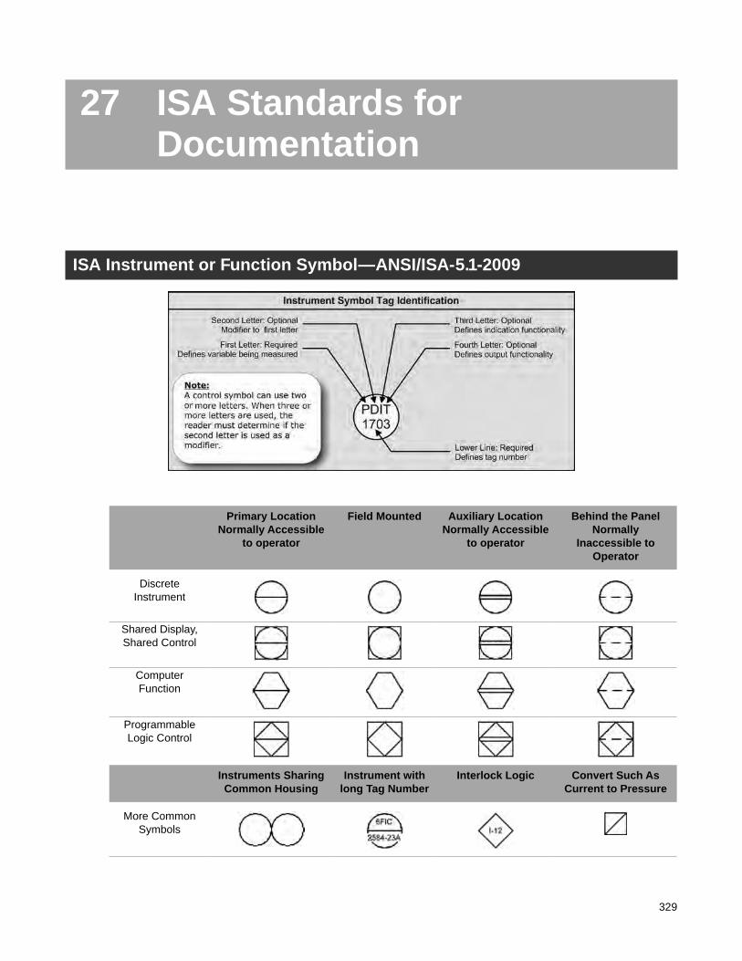
329
27 ISA Standards for Documentation
ISA Instrument or Function Symbol—ANSI/ISA-5 .1-2009
Primary Location Normally Accessible
to operator
Field Mounted Auxiliary Location Normally Accessible
to operator
Behind the Panel Normally
Inaccessible to Operator
Discrete Instrument
Shared Display, Shared Control
Computer Function
Programmable Logic Control
Instruments Sharing Common Housing
Instrument with long Tag Number
Interlock Logic Convert Such As Current to Pressure
More Common Symbols
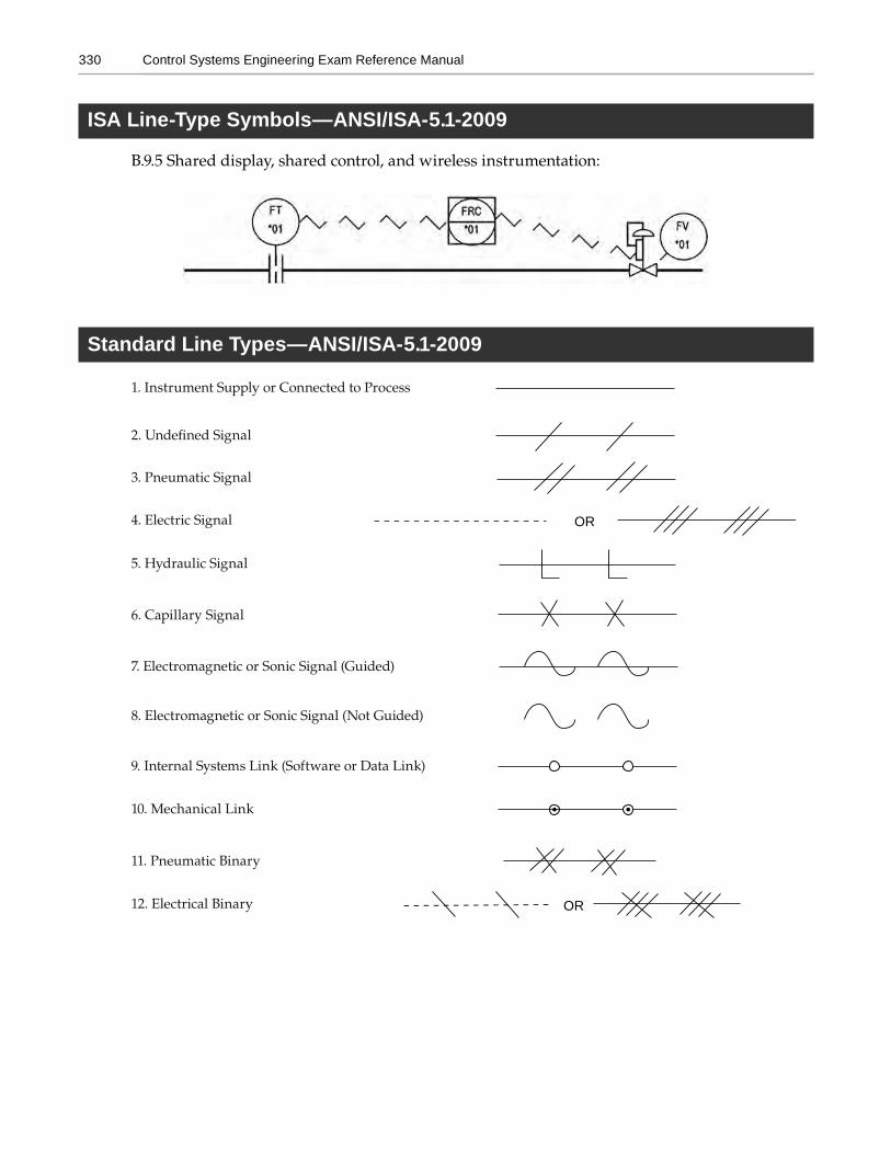
330 Control Systems Engineering Exam Reference Manual
ISA Line-Type Symbols—ANSI/ISA-5 .1-2009
B.9.5 Shared display, shared control, and wireless instrumentation:
Standard Line Types—ANSI/ISA-5 .1-2009
1. Instrument Supply or Connected to Process
3. Pneumatic Signal
4. Electric Signal
5. Hydraulic Signal
6. Capillary Signal
7. Electromagnetic or Sonic Signal (Guided)
8. Electromagnetic or Sonic Signal (Not Guided)
9. Internal Systems Link (Software or Data Link)
10. Mechanical Link
11. Pneumatic Binary
12. Electrical Binary
OR
OR
351
28 Overview of Safety Instrumented Systems
Overview of Process Safety and Shutdown
On the CSE exam, there will be questions on safety instrumented systems (SISs) and safety integ-rity levels (SILs). We will discuss some of the calculations and data you may encounter on the test.
SISs
US Occupational Safety and Health Administration (OSHA) law incorporates as a guideline that “good engineering practice” will be used in evaluating and engineering SISs. This means that the program follows the codes and standards published by such organizations as the American Society of Mechanical Engineers (ASME), American Petroleum Institute (API), American National Standards Institute (ANSI), National Fire Protection Association (NFPA), American Society for Testing and Materials (ASTM), National Board of Boiler and Pressure Vessel Inspectors (NBBI), and International Society of Automation (ISA). Other countries have similar requirements.
ANSI/ISA-S84.00.01-2003, (IEC 61511 Mod), Application of Safety Instrumented Systems for the Process Industries, (referred to as IEC 61511/ISA-84 in this book) addresses the application of SISs to take a process to a safe state when predetermined conditions are violated, such as set points for pressure, temperature, and level. Its objective is to define requirements for SISs. SISs are also called emergency shutdown systems, safety shutdown systems, and safety interlock systems. SISs provide safety control functions and complement the basic process control system (BPCS), which provides normal process control. IEC 61511/ISA-84 address the entire life cycle for SISs, and compliance with the standard requires a significant effort.
Complying with IEC 61511/ISA-84
OSHA endorsed IEC 61511/ISA-84 as a “national consensus standard” in a March 23, 2000, OSHA letter to ISA. This letter states that the standard is considered “a recognized and generally accepted good engineering practice” for SISs. Paragraph (d)(3)(ii) of the process safety management (PSM) standard specifies, “The employer shall document that equipment complies with recognized and generally accepted good engineering practices.” The letter states that in evaluating whether an employer’s engineering practices with respect to SISs comply with PSM, OSHA would consider, among other factors, whether the employer meets the requirements of IEC 61511/ISA-84.
352 Control Systems Engineering Exam Reference Manual
In the letter, OSHA states that it is also important to note that there are a large percentage of processes that are not covered by PSM, which may include SISs covered by the standard. OSHA states that “the employer may be in violation of the General Duty Clause, Section 5(a)(1) of the OSH Act, if SISs are utilized that do not conform with IEC 61511/ISA-84, and hazards exist related to the SISs that could seriously harm employees”. Consequently, this means that companies must comply with IEC 61511/ISA-84, not only for PSM-covered processes, but also for other processes that use SISs where hazards to personnel may be present.
Regardless of regulatory requirements, IEC 61511/ISA-84 is an internationally recognized standard and represents good engineering practice.
Other Codes Related to SIS• NFPA 85 – Boiler and Combustion Systems Hazard Code
• NFPA 86 – Standard for Ovens and Furnaces
• IEC 61508 – Functional Safety: Safety-Related Systems
• IEC 61511 – Functional Safety: Safety Instrumented Systems for the Process Industry Sector
• ANSI/ISA S84.01 – Application of Safety Instrumented Systems for the Process Industries
ISA and OSHA Letter Defining the Requirements for Implementation of SIS
• Standard Number: 1910.119
This letter constitutes OSHA’s interpretation only of the requirements discussed and may not be applicable to any situation not delineated within the original correspondence.
November 29, 2005
Ms. Lois M. Ferson Manager of Standards Services ISA 67 Alexandria Drive P.O. Box 12277 Research Triangle Park, NC 27709
Dear Ms. Ferson:
Thank you for your October 25, 2004 letter to the Occupational Safety and Health Administration (OSHA), on behalf of the Instrumentation, Systems, and Automation Society (ISA), regarding a consensus standard jointly issued by the American National Standards Institute (ANSI) and ISA that may be applied under OSHA’s Process Safety Management (PSM) standard, 29 CFR 1910.119. We apologize for the delay in our response.
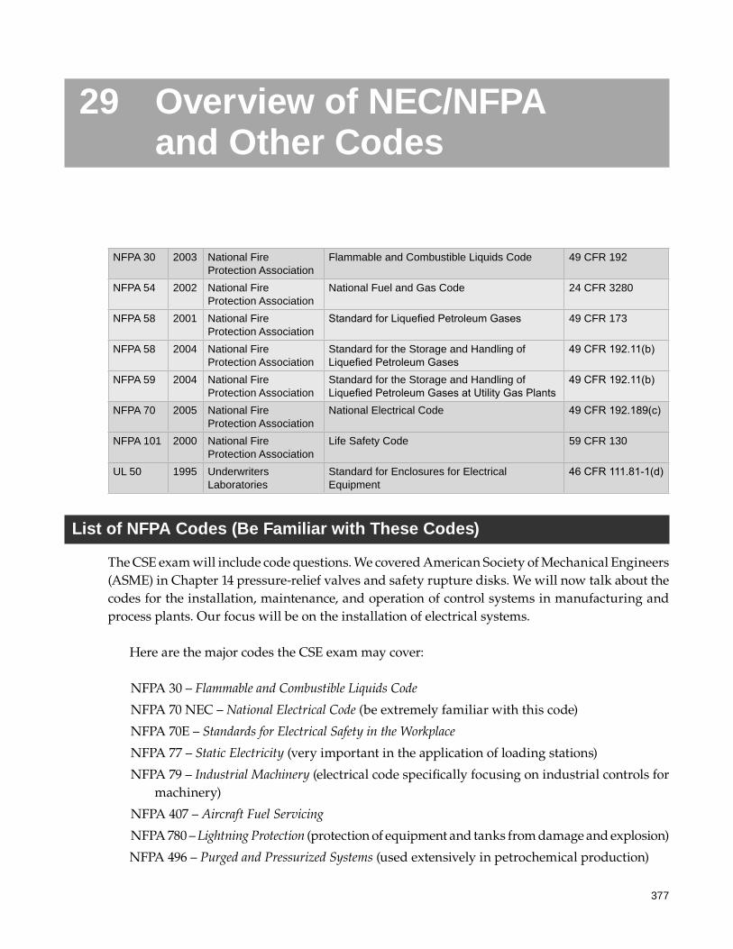
377
29 Overview of NEC/NFPA and Other Codes
List of NFPA Codes (Be Familiar with These Codes)
The CSE exam will include code questions. We covered American Society of Mechanical Engineers (ASME) in Chapter 14 pressure-relief valves and safety rupture disks. We will now talk about the codes for the installation, maintenance, and operation of control systems in manufacturing and process plants. Our focus will be on the installation of electrical systems.
Here are the major codes the CSE exam may cover:
NFPA 30 – Flammable and Combustible Liquids Code
NFPA 70 NEC – National Electrical Code (be extremely familiar with this code)
NFPA 70E – Standards for Electrical Safety in the Workplace
NFPA 77 – Static Electricity (very important in the application of loading stations)
NFPA 79 – Industrial Machinery (electrical code specifically focusing on industrial controls for machinery)
NFPA 407 – Aircraft Fuel Servicing
NFPA 780 – Lightning Protection (protection of equipment and tanks from damage and explosion)
NFPA 496 – Purged and Pressurized Systems (used extensively in petrochemical production)
NFPA 30 2003 National Fire Protection Association
Flammable and Combustible Liquids Code 49 CFR 192
NFPA 54 2002 National Fire Protection Association
National Fuel and Gas Code 24 CFR 3280
NFPA 58 2001 National Fire Protection Association
Standard for Liquefied Petroleum Gases 49 CFR 173
NFPA 58 2004 National Fire Protection Association
Standard for the Storage and Handling of Liquefied Petroleum Gases
49 CFR 192.11(b)
NFPA 59 2004 National Fire Protection Association
Standard for the Storage and Handling of Liquefied Petroleum Gases at Utility Gas Plants
49 CFR 192.11(b)
NFPA 70 2005 National Fire Protection Association
National Electrical Code 49 CFR 192.189(c)
NFPA 101 2000 National Fire Protection Association
Life Safety Code 59 CFR 130
UL 50 1995 Underwriters Laboratories
Standard for Enclosures for Electrical Equipment
46 CFR 111.81-1(d)

378 Control Systems Engineering Exam Reference Manual
All the above listed standards are referred to and may be required by the word “shall” to meet the federally required compliance. 49 CFR 195.405(a) (API Standard 2003 Protection Against Ignitions Arising Out of Static, Lightning, and Stray Currents) and 49 CFR 192 (NFPA 30, Flammable and Combustible Liquids Code) are both required by the NEC, NFPA 70.
NFPA 70 – NEC
Be familiar with the NEC (NFPA 70) National Electrical Code Handbook, or a book of equal infor-mation. Most, if not all, the information and tables required for performing the calculations on the CSE exam are in this manual. The handbook contains information needed for motors, hazard-ous locations, National Electrical Manufacturers Association (NEMA) classifications, and tem-perature group ratings. The NEC handbook contains information about group classifications and auto-ignition temperature ratings of flammable gases and vapors (reprints from NFPA 497M).
Most states require an inspection of plant installations by a local electrical inspector (authority having jurisdiction—AHJ). In Article 100 of the 2014 NEC, the term authority having jurisdiction is defined as “an organization, office, or individual responsible for enforcing the requirements of a code or standard, or for approving equipment, materials, an installation, or a procedure.”
The following is a list of tables that may be used on the CSE exam.
• Table 310-16 Conductor ampacities in raceways, cable or earth
• Table 430-147 Motor currents for single-phase motors
• Table 430-150 Motor currents for three-phase motors
• 500-2 List of TYPE X, Y, Z purging of enclosures (in handbook only)
• 500-3 Special precautions, group classifications of gases and vapors
• 500-3 List of gases and vapors, with their group ratings (in handbook only)
• 504-X Intrinsically Safe Systems (review this section)
• 504-50 Handbook, diagrams of intrinsically safe barriers
• 725 Class 1, Class 2, Class 3 Remote Control Circuits
• 800 Communications Circuits
• Chapter 9—Table 8 Conductor properties and DC resistance
• Chapter 9—Table 9 AC resistance for 600-volt cables
Voltage Drop Calculations
Voltage drop will also probably be on the CSE exam. Voltage drop is just Ohm’s law.
VL
I RD =⋅
2
1000i i ( ;from NEC table) for DC
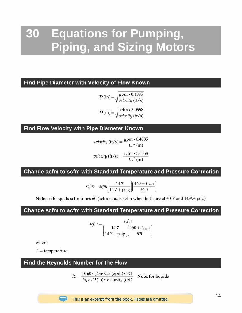
411
30 Equations for Pumping, Piping, and Sizing Motors
Find Pipe Diameter with Velocity of Flow Known
IDvelocity
( ).( )
in/
=gpm
ft si 0 4085
IDvelocity
( ).( )
in/
=acfm
ft si 3 0558
Find Flow Velocity with Pipe Diameter Known
velocityID
( ).
( )ft s
gpm/
in=
i 0 40852
velocityID
( ).
( )ft s
acfm/
in=
i 3 05582
Change acfm to scfm with Standard Temperature and Pressure Correction
scfm acfmT
=+
+
14 714 7
460520
.. psig
deg F
Note: scfh equals scfm times 60 (acfm equals scfm when both are at 60°F and 14.696 psia)
Change scfm to acfm with Standard Temperature and Pressure Correction
acfmscfm
T=
+
+
14 714 7
460520
..
deg
psig F
where
T = temperature
Find the Reynolds Number for the Flow
R =flow rate SG
Pipe ID Viscosity e
3160 gpmcSt
i ii
( )( ) ( )in
Notte: for liquids
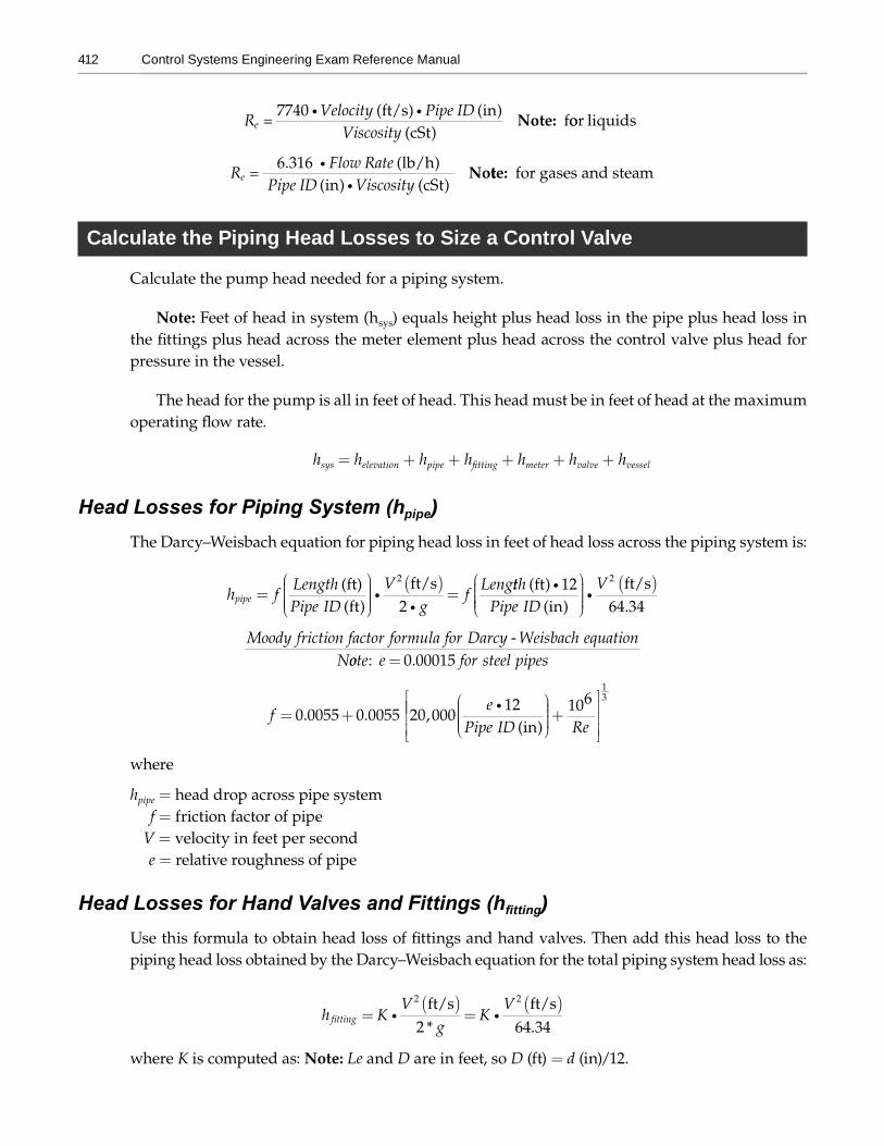
412 Control Systems Engineering Exam Reference Manual
R =Velocity Pipe ID
Viscositye
7740 i i( ) ( )( )
ft scSt
f/ in
Note: oor liquids
R = Flow Rate
Pipe ID Viscosity e
6.316cSt
ii
( )( ) ( )
lb/hin
Notte: for gases and steam
Calculate the Piping Head Losses to Size a Control Valve
Calculate the pump head needed for a piping system.
Note: Feet of head in system (hsys) equals height plus head loss in the pipe plus head loss in the fittings plus head across the meter element plus head across the control valve plus head for pressure in the vessel.
The head for the pump is all in feet of head. This head must be in feet of head at the maximum operating flow rate.
hsys = helevation + hpipe + hfitting + hmeter + hvalve + hvessel
Head Losses for Piping System (hpipe)The Darcy–Weisbach equation for piping head loss in feet of head loss across the piping system is:
h fLengthPipe ID
Vg
fLeng
pipe =
( )=
(( )ft)
ftft/s
ii
2
2tth
Pipe IDV( )
( ) .ft
inft/i
i12
64 34
2
( )s
Moody friction factor formula for Darcy Weisbach equationN
-oote e for steel pipes: . = 0 00015
fe
Pipe ID= +
+
0 0055 0 0055 20 000
12 106. . ,
( )i in Re
13
where
hpipe = head drop across pipe systemf = friction factor of pipe
V = velocity in feet per seconde = relative roughness of pipe
Head Losses for Hand Valves and Fittings (hfitting)Use this formula to obtain head loss of fittings and hand valves. Then add this head loss to the piping head loss obtained by the Darcy–Weisbach equation for the total piping system head loss as:
h KV
gK
Vfitting =
( )=
( )i i
2 2
2 64 34ft s ft s/ /* .
where K is computed as: Note: Le and D are in feet, so D (ft) = d (in)/12.
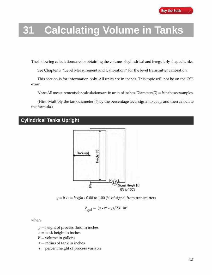
417
31 Calculating Volume in Tanks
The following calculations are for obtaining the volume of cylindrical and irregularly shaped tanks.
See Chapter 8, “Level Measurement and Calibration,” for the level transmitter calibration.
This section is for information only. All units are in inches. This topic will not be on the CSE exam.
Note: All measurements for calculations are in units of inches. Diameter (D) = h in these examples.
(Hint: Multiply the tank diameter (h) by the percentage level signal to get y, and then calculate the formula.)
Cylindrical Tanks Upright
y h= =i is height 0.00 to 1.00 (% of signal from transmitter)
V r ygal ( )/231 in2 3= π i i
where
y = height of process fluid in inchesh = tank height in inches
V = volume in gallonsr = radius of tank in inchess = percent height of process variable
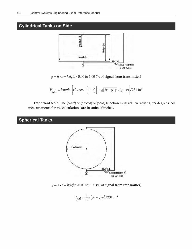
418 Control Systems Engineering Exam Reference Manual
Cylindrical Tanks on Side
y h s height= =i i 0.00 to 1.00 (% of signal from transmitter)
V length rgal /22= i i icos ( )− −
+ −( ) −
1 1 2yr
r y y y r 331 in3
Important Note: The (cos−1) or (arccos) or (acos) function must return radians, not degrees. All measurements for the calculations are in units of inches.
Spherical Tanks
y h s height= =i i 0.00 to 1.00 (% of signal from transmitter)
V r y ygal13
3 /231 in2 3= ( )π −
421
32 Exam Sample Questions
Sample Questions
1. At 433°F, a type J thermocouple with a 32°F reference junction (ice bath) will produce anoutput in millivolts (mV) that is most nearly equal to:
A. 9.04 mVB. 10.51 mVC. 12.05 mVD. 17.79 mV
2. The flow of water in a 6-inch pipe is measured with an orifice plate and differential pres-sure transmitter. At a flow rate of 200 gpm, the differential pressure is 35 in of water. At aflow rate of 312 gpm, the differential pressure will be approximately equal to:
A. 16.4 in wcB. 32.5 in wcC. 85.4 in wcD. 100 in wc
3. A tank level is measured using a differential pressure transmitter and a bubbler tube. Thetank is vented to atmosphere. The bubbler tube is 1 ft from the bottom of the tank, andthe tank wall is 20 ft high. A 0–10 psig differential pressure gauge, accurate to 0.25% offull scale, is connected to the bubbler tube connection at the high side of the transmitter.The low-pressure side is connected to the tank top. With the tank containing liquid witha specific gravity (SG) of 1.1 and the level in the tank at 16 ft, the gauge reading in poundsper square inch (psi) is most nearly equal to:
A. 4.80B. 9.35C. 13.00D. 7.10
4. Which of the following practices is important in routing optic cable?
A. Laying cable in trays with high-horsepower motor wiring should be avoided.B. Conduit fittings that require small radius bends should be avoided.C. Overhead runs on messenger wires should be limited to 75 ft.D. Underground fiber-optic runs must be covered with concrete.
422 Control Systems Engineering Exam Reference Manual
5. Compared to a control loop with no dead time (pure time delay), a control loop with anappreciable dead time tends to require:
A. Less proportional gain and less integral actionB. More proportional gain and less integral actionC. More proportional gain and more integral actionD. Less proportional gain and more integral action
6. The definition and classification of hazardous areas for the purpose of wiring and electri-cal equipment is found in codes published by:
A. National Fire Protection AssociationB. International Society of AutomationC. Electric Power Research InstituteD. Occupational Safety and Health Administration
7. Given the following data for liquid flow:Flow rate: 0–200 gpmWater at: 125°F and 75 psiaPipe size: 4-inch, schedule 40
The orifice bore for a pressure differential range of 100 in of water is most nearly equal to:
A. 2.33 inB. 3.50 inC. 1.50 inD. 0.75 in
8. A control valve is to be sized for the following conditions:Liquid flow: 50 gpmSpecific gravity: 0.81Inlet pressure: 240 psigDelta pressure drop of across the valve: 10 psi
The required flow coefficient (Cv) for the valve will most nearly be:
A. 10.4B. 14.2C. 22.0D. 35.5
9. A control valve is to be sized for the following service conditions, saturated steam:Maximum flow rate: 30,000 lb/hP1 (upstream pressure): 40 psiaP2 (downstream pressure): 30 psia
439
33 Guide to the Fisher Control Valve Handbook
The Fisher Control Valve Handbook from Emerson is a supplement book with many worked examples.
Purchasing this book or printing it out is highly recommended.
The handbook can help aid in study for the CSE exam. The information and tables in the Fisher Control Valve Handbook will be constantly referenced. I have repeated the most common data from the book needed for the CSE exam. The book is not required, but it is recommended and may be downloaded in PDF format from the Fisher Controls public website at the following address:
https://www.emerson.com/documents/automation/control-valve-handbook-en-3661206.pdf
If you wish to obtain a hard copy of the handbook, the Fisher Control Valve Handbook can be acquired for free, or for about $20, from your local instrumentation supplier. The book is also available from Brown’s Technical Book Shop, 1517 San Jacinto, Houston, Texas, 77002. http://www.browntechnical.org.
I suggest tabbing the handbook for quick reference.
Important Sections to Review
• Chapter 3 – Valve and Actuator Types
• Chapter 5 – USA Regulatory Requirement for Fugitive Emissions
• Chapter 5 – Control Valve Selection (and sizing)
Important Pages to Possibly Tab
Valve and Materials Selection• Chart for Test Frequency for Valves Leaking 500 ppm
• Sliding-Stem Valve Environmental Packing Selection
• Rotary Valve Environmental Packing Selection
• Designations for the High Nickel Alloys
440 Control Systems Engineering Exam Reference Manual
Pressure-Temperature Ratings for Standard Class
• Cast Carbon Steel (ASTM A216 Grade WCC)
• Cast Chromium-Molybdenum Steel (ASTM A217 Grade WC9)
• Cast Chromium-Molybdenum Steel (ASTM A217 Grade C5)
• Cast Type 304L Stainless Steel (ASTM A351 Grade CF3)
• Cast Type 316 Stainless Steel (ASTM A351 Grade CF8M)
• Cast Type 317 Stainless Steel (ASTM A479 Grade UNS S31700)
• Cast Iron (ASTM A126)
• Cast Bronze Valves (ASTM B61 and B62)
Valve Trim Material Temperature Limits
Ambient Temperature Corrosion information
Elastomer Information
Application of Valves for Liquid Level Systems
Application of Valves for Flow Control Processes
Actuator Sizing Methods• Typical Packing Friction Values
• Actuator Force Calculations
• Typical Rotary Shaft Valve Torque Factors (V-Notch Ball Valve)
• Typical Rotary Shaft Valve Torque Factors (High-Performance Butterfly Valve)
• Packing Selection Guidelines for Sliding-Stem Valves (100 ppm)
• Packing Selection Guidelines for Rotary Valves (500 ppm)
Valve Sizing Methods• Valve Sizing Procedure
• Abbreviations and Terminology
• Equation Constants
• Determining qMAX (the Maximum Flow Rate)
• Determining PMAX (the Allowable Sizing Pressure Drop)
• Liquid Sizing Sample Problem
• Sizing Coefficients (Cv, XT) for Single-Ported Globe Valve Bodies
• Sizing Coefficients (Cv, XT) for Rotary Shaft Valve Bodies
Electrical Apparatus• NEMA Enclosure Ratings and Definitions
• Hazardous Location Classification
• IEC Temperature Codes (Temperature Ratings)
• NEMA and IEC Enclosure Rating Comparison
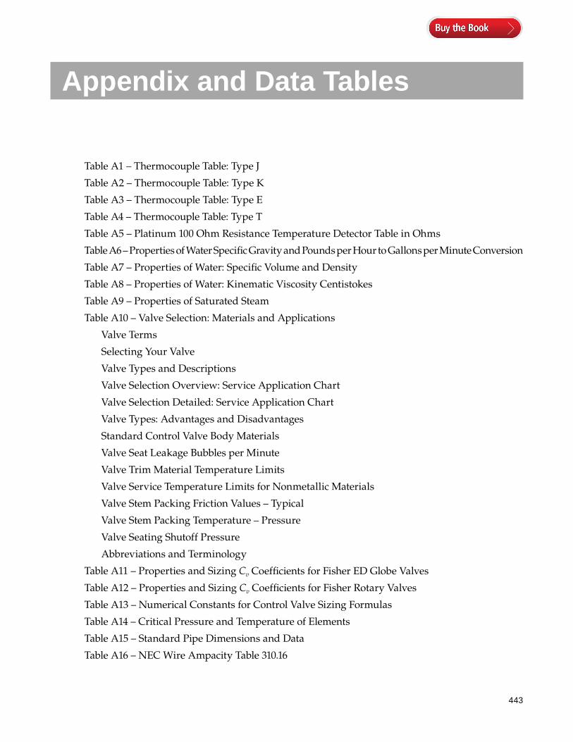
443
Appendix and Data Tables
Table A1 – Thermocouple Table: Type J
Table A2 – Thermocouple Table: Type K
Table A3 – Thermocouple Table: Type E
Table A4 – Thermocouple Table: Type T
Table A5 – Platinum 100 Ohm Resistance Temperature Detector Table in Ohms
Table A6 – Properties of Water Specific Gravity and Pounds per Hour to Gallons per Minute Conversion
Table A7 – Properties of Water: Specific Volume and Density
Table A8 – Properties of Water: Kinematic Viscosity Centistokes
Table A9 – Properties of Saturated Steam
Table A10 – Valve Selection: Materials and Applications
Valve Terms
Selecting Your Valve
Valve Types and Descriptions
Valve Selection Overview: Service Application Chart
Valve Selection Detailed: Service Application Chart
Valve Types: Advantages and Disadvantages
Standard Control Valve Body Materials
Valve Seat Leakage Bubbles per Minute
Valve Trim Material Temperature Limits
Valve Service Temperature Limits for Nonmetallic Materials
Valve Stem Packing Friction Values – Typical
Valve Stem Packing Temperature – Pressure
Valve Seating Shutoff Pressure
Abbreviations and Terminology
Table A11 – Properties and Sizing Cv Coefficients for Fisher ED Globe Valves
Table A12 – Properties and Sizing Cv Coefficients for Fisher Rotary Valves
Table A13 – Numerical Constants for Control Valve Sizing Formulas
Table A14 – Critical Pressure and Temperature of Elements
Table A15 – Standard Pipe Dimensions and Data
Table A16 – NEC Wire Ampacity Table 310.16
444 Control Systems Engineering Exam Reference Manual
Table A17 – NEC Conductor Properties and Impedance
Table A18 – NEC Full-Load Motor Currents
Table A19 – NEC Grounding and Bonding Conductors
Table A20 – Specific Gravity and Gas Constants: Some Common Gases
Table A21 – Specific Gravity: Common Fluids
Table A22 – Kinematic Viscosity: Common Fluids
Table A23 –Absolute Viscosity: Common Liquids
Table A24 –Absolute Viscosity Common Gases
Table A25 – Density of Elements in English and Metric Units
Table A26 – Metric Conversion Tables
Table A27 – Standard Conditions and Gas Laws
Table A28 – Head Loss in Piping Systems
Table A29 – Maximal Flow Velocity in Pipes
Table A30 – Pressure Vapor Chart of Common Liquids

445Appendix and Data Tables
Table A1 – Thermocouple Table: Type J
Thermoelectric Voltage in Millivolts
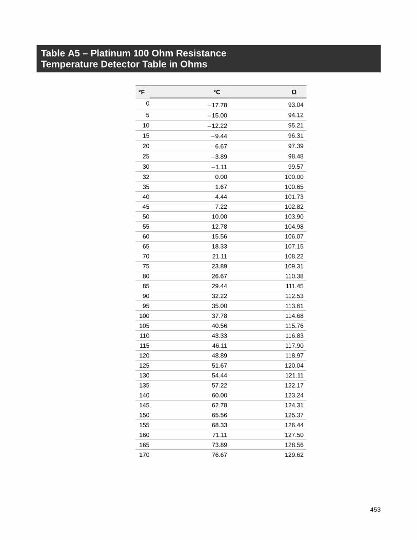
453
Table A5 – Platinum 100 Ohm Resistance Temperature Detector Table in Ohms
°F °C Ω
0 −17.78 93.045 −15.00 94.12
10 −12.22 95.2115 −9.44 96.3120 −6.67 97.3925 −3.89 98.4830 −1.11 99.5732 0.00 100.0035 1.67 100.6540 4.44 101.7345 7.22 102.8250 10.00 103.9055 12.78 104.9860 15.56 106.0765 18.33 107.1570 21.11 108.2275 23.89 109.3180 26.67 110.3885 29.44 111.4590 32.22 112.5395 35.00 113.61
100 37.78 114.68105 40.56 115.76110 43.33 116.83115 46.11 117.90120 48.89 118.97125 51.67 120.04130 54.44 121.11135 57.22 122.17140 60.00 123.24145 62.78 124.31150 65.56 125.37155 68.33 126.44160 71.11 127.50165 73.89 128.56170 76.67 129.62
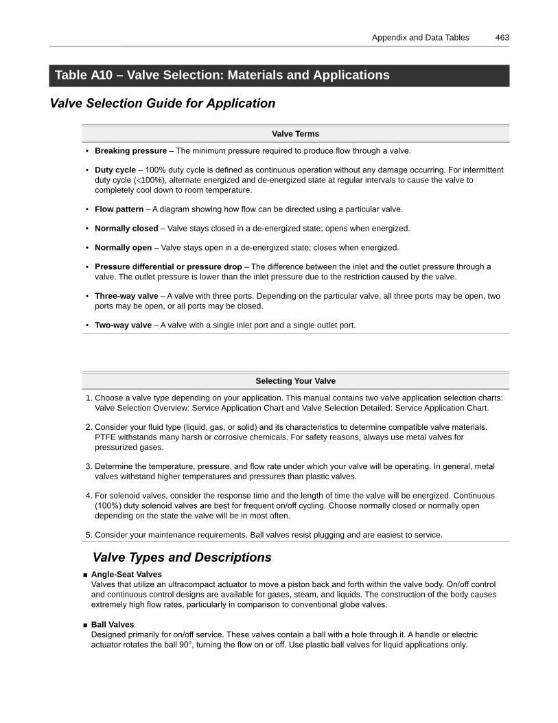
463Appendix and Data Tables
Table A10 – Valve Selection: Materials and Applications
Valve Selection Guide for Application
Valve Terms
• Breaking pressure – The minimum pressure required to produce flow through a valve.
• Duty cycle – 100% duty cycle is defined as continuous operation without any damage occurring. For intermittentduty cycle (<100%), alternate energized and de-energized state at regular intervals to cause the valve tocompletely cool down to room temperature.
• Flow pattern – A diagram showing how flow can be directed using a particular valve.
• Normally closed – Valve stays closed in a de-energized state; opens when energized.
• Normally open – Valve stays open in a de-energized state; closes when energized.
• Pressure differential or pressure drop – The difference between the inlet and the outlet pressure through avalve. The outlet pressure is lower than the inlet pressure due to the restriction caused by the valve.
• Three-way valve – A valve with three ports. Depending on the particular valve, all three ports may be open, twoports may be open, or all ports may be closed.
• Two-way valve – A valve with a single inlet port and a single outlet port.
Selecting Your Valve
1. Choose a valve type depending on your application. This manual contains two valve application selection charts:Valve Selection Overview: Service Application Chart and Valve Selection Detailed: Service Application Chart.
2. Consider your fluid type (liquid, gas, or solid) and its characteristics to determine compatible valve materials.PTFE withstands many harsh or corrosive chemicals. For safety reasons, always use metal valves forpressurized gases.
3. Determine the temperature, pressure, and flow rate under which your valve will be operating. In general, metalvalves withstand higher temperatures and pressures than plastic valves.
4. For solenoid valves, consider the response time and the length of time the valve will be energized. Continuous(100%) duty solenoid valves are best for frequent on/off cycling. Choose normally closed or normally opendepending on the state the valve will be in most often.
5. Consider your maintenance requirements. Ball valves resist plugging and are easiest to service.
Valve Types and Descriptions Angle-Seat Valves
Valves that utilize an ultracompact actuator to move a piston back and forth within the valve body. On/off control and continuous control designs are available for gases, steam, and liquids. The construction of the body causes extremely high flow rates, particularly in comparison to conventional globe valves.
Ball ValvesDesigned primarily for on/off service. These valves contain a ball with a hole through it. A handle or electric actuator rotates the ball 90°, turning the flow on or off. Use plastic ball valves for liquid applications only.
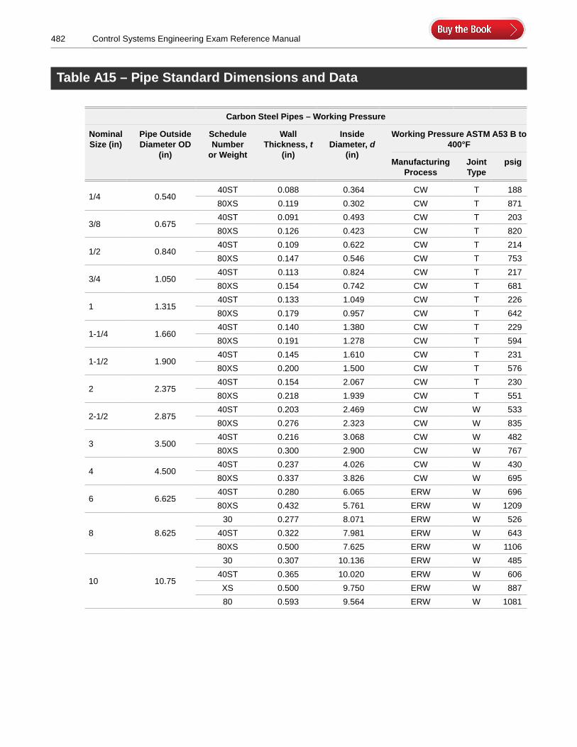
482 Control Systems Engineering Exam Reference Manual
Table A15 – Pipe Standard Dimensions and Data
Carbon Steel Pipes – Working Pressure
Nominal Size (in)
Pipe Outside Diameter OD
(in)
Schedule Number
or Weight
Wall Thickness, t
(in)
Inside Diameter, d
(in)
Working Pressure ASTM A53 B to 400°F
Manufacturing Process
Joint Type
psig
1/4 0.54040ST 0.088 0.364 CW T 18880XS 0.119 0.302 CW T 871
3/8 0.67540ST 0.091 0.493 CW T 20380XS 0.126 0.423 CW T 820
1/2 0.84040ST 0.109 0.622 CW T 21480XS 0.147 0.546 CW T 753
3/4 1.05040ST 0.113 0.824 CW T 21780XS 0.154 0.742 CW T 681
1 1.31540ST 0.133 1.049 CW T 22680XS 0.179 0.957 CW T 642
1-1/4 1.66040ST 0.140 1.380 CW T 22980XS 0.191 1.278 CW T 594
1-1/2 1.90040ST 0.145 1.610 CW T 23180XS 0.200 1.500 CW T 576
2 2.37540ST 0.154 2.067 CW T 23080XS 0.218 1.939 CW T 551
2-1/2 2.87540ST 0.203 2.469 CW W 53380XS 0.276 2.323 CW W 835
3 3.50040ST 0.216 3.068 CW W 48280XS 0.300 2.900 CW W 767
4 4.50040ST 0.237 4.026 CW W 43080XS 0.337 3.826 CW W 695
6 6.62540ST 0.280 6.065 ERW W 69680XS 0.432 5.761 ERW W 1209
8 8.62530 0.277 8.071 ERW W 526
40ST 0.322 7.981 ERW W 64380XS 0.500 7.625 ERW W 1106
10 10.75
30 0.307 10.136 ERW W 48540ST 0.365 10.020 ERW W 606XS 0.500 9.750 ERW W 88780 0.593 9.564 ERW W 1081
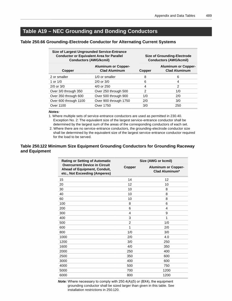
489Appendix and Data Tables
Table A19 – NEC Grounding and Bonding Conductors
Table 250 .66 Grounding-Electrode Conductor for Alternating Current Systems
Table 250 .122 Minimum Size Equipment Grounding Conductors for Grounding Raceway and Equipment
Size of Largest Ungrounded Service-Entrance Conductor or Equivalent Area for Parallel
Conductors (AWG/kcmil)Size of Grounding-Electrode
Conductors (AWG/kcmil)
CopperAluminum or Copper-
Clad Aluminum CopperAluminum or Copper-
Clad Aluminum
2 or smaller 1/0 or smaller 8 61 or 1/0 2/0 or 3/0 6 42/0 or 3/0 4/0 or 250 4 2Over 3/0 through 350 Over 250 through 500 2 1/0Over 350 through 600 Over 500 through 900 1/0 2/0Over 600 through 1100 Over 900 through 1750 2/0 3/0Over 1100 Over 1750 3/0 250
Notes:1. Where multiple sets of service-entrance conductors are used as permitted in 230.40.
Exception No. 2: The equivalent size of the largest service-entrance conductor shall bedetermined by the largest sum of the areas of the corresponding conductors of each set.
2. Where there are no service-entrance conductors, the grounding-electrode conductor sizeshall be determined by the equivalent size of the largest service-entrance conductor requiredfor the load to be served.
Rating or Setting of Automatic Overcurrent Device in Circuit Ahead of Equipment, Conduit, etc ., Not Exceeding (Amperes)
Size (AWG or kcmil)
Copper Aluminum or Copper-Clad Aluminum*
15 14 1220 12 1030 10 840 10 860 10 8100 8 6200 6 4300 4 9400 3 1500 2 1/0600 1 2/0800 1/0 3/01000 2/0 4.01200 3/0 2501600 4/0 3502000 250 4002500 350 6003000 400 6004000 500 7505000 700 12006000 800 1200
Note: Where necessary to comply with 250.4(A)(5) or (BX4), the equipment grounding conductor shall be sized larger than given in this table. See installation restrictions in 250.120.
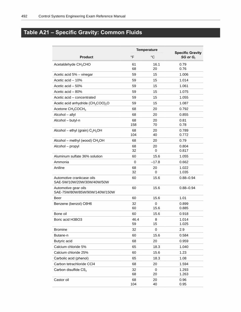
492 Control Systems Engineering Exam Reference Manual
Table A21 – Specific Gravity: Common Fluids
Product
TemperatureSpecific Gravity
SG or Gf°F °C
Acetaldehyde CH3CHO 6168
16.120
0.790.76
Acetic acid 5% – vinegar 59 15 1.006Acetic acid – 10% 59 15 1.014Acetic acid – 50% 59 15 1.061Acetic acid – 80% 59 15 1.075Acetic acid – concentrated 59 15 1.055Acetic acid anhydride (CH3COO)2O 59 15 1.087Acetone CH3COCH3 68 20 0.792Alcohol – allyl 68 20 0.855Alcohol – butyl-n 68
1582070
0.810.78
Alcohol – ethyl (grain) C2H5OH 68104
2040
0.7890.772
Alcohol – methyl (wood) CH3OH 68 20 0.79Alcohol – propyl 68
32200
0.8040.817
Aluminum sulfate 36% solution 60 15.6 1.055Ammonia 0 –17.8 0.662Aniline 68
32200
1.0221.035
Automotive crankcase oilsSAE-5W/10W/20W/30W/40W/50W
60 15.6 0.88–0.94
Automotive gear oilsSAE-75W/80W/85W/90W/140W/150W
60 15.6 0.88–0.94
Beer 60 15.6 1.01Benzene (benzol) C6H6 32
600
15.60.8990.885
Bone oil 60 15.6 0.918Boric acid H3BO3 46.4
598
151.0141.025
Bromine 32 0 2.9Butane-n 60 15.6 0.584Butyric acid 68 20 0.959Calcium chloride 5% 65 18.3 1.040Calcium chloride 25% 60 15.6 1.23Carbolic acid (phenol) 65 18.3 1.08Carbon tetrachloride CCl4 68 20 1.594Carbon disulfide CS2 32
680
201.2931.263
Castor oil 68104
2040
0.960.95
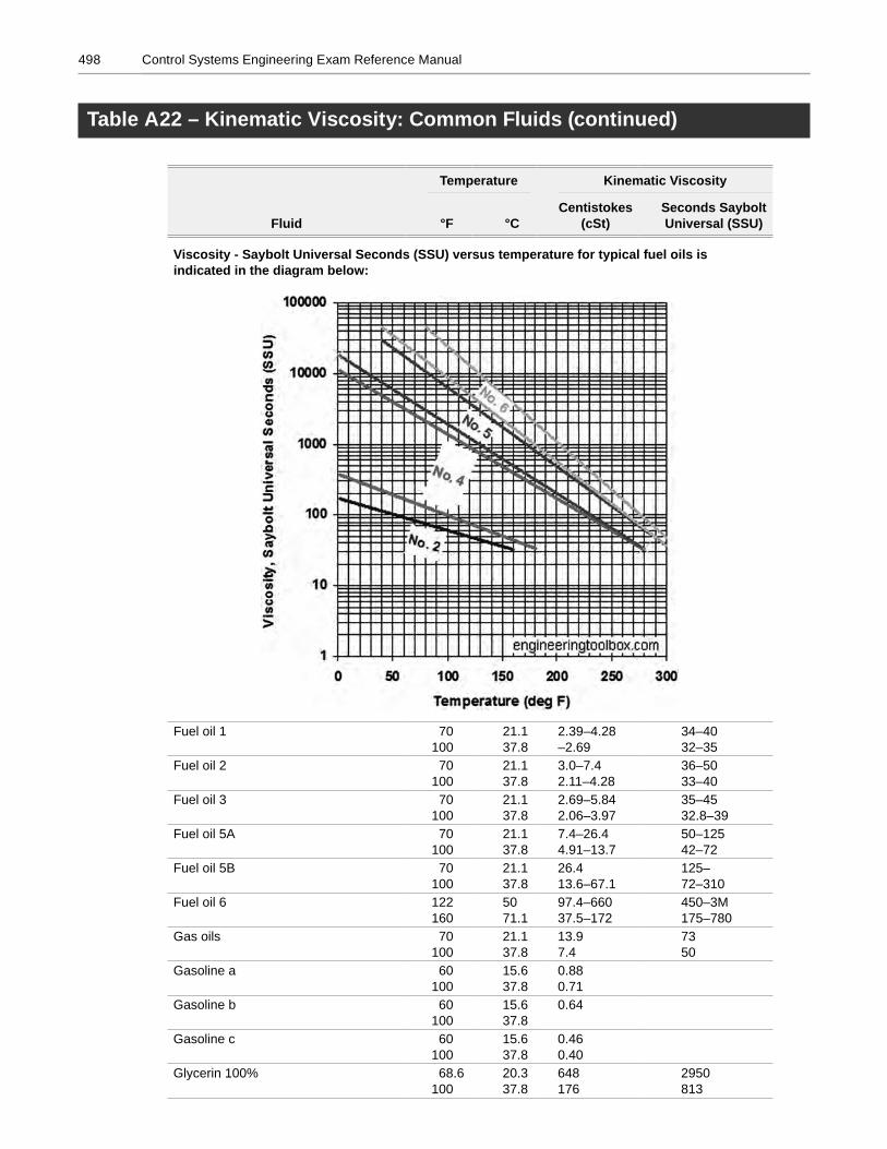
498 Control Systems Engineering Exam Reference Manual
Table A22 – Kinematic Viscosity: Common Fluids (continued)
Fluid
Temperature Kinematic Viscosity
°F °CCentistokes
(cSt)Seconds Saybolt Universal (SSU)
Viscosity - Saybolt Universal Seconds (SSU) versus temperature for typical fuel oils is indicated in the diagram below:
Fuel oil 1 70100
21.137.8
2.39–4.28–2.69
34–4032–35
Fuel oil 2 70100
21.137.8
3.0–7.42.11–4.28
36–5033–40
Fuel oil 3 70100
21.137.8
2.69–5.842.06–3.97
35–4532.8–39
Fuel oil 5A 70100
21.137.8
7.4–26.44.91–13.7
50–12542–72
Fuel oil 5B 70100
21.137.8
26.413.6–67.1
125–72–310
Fuel oil 6 122160
5071.1
97.4–66037.5–172
450–3M175–780
Gas oils 70100
21.137.8
13.97.4
7350
Gasoline a 60100
15.637.8
0.880.71
Gasoline b 60100
15.637.8
0.64
Gasoline c 60100
15.637.8
0.460.40
Glycerin 100% 68.6100
20.337.8
648176
2950813
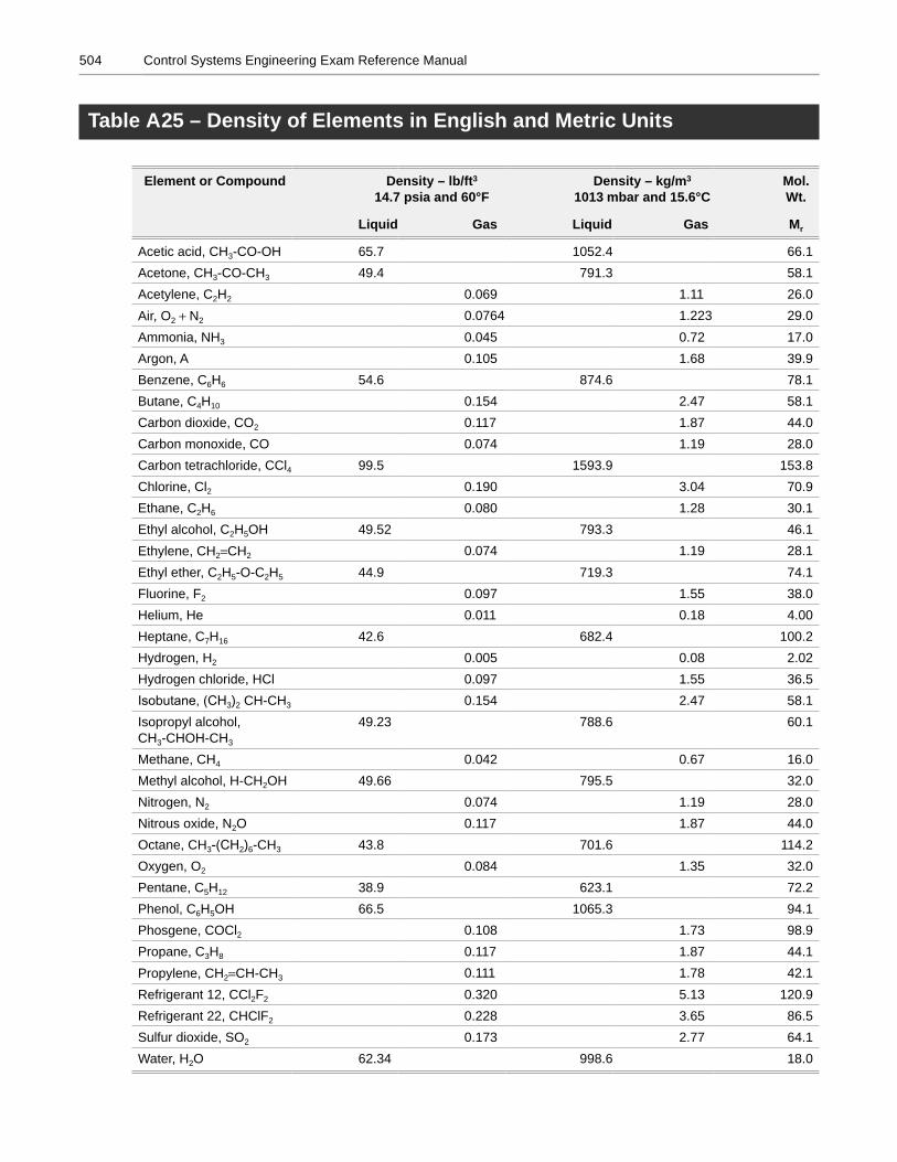
504 Control Systems Engineering Exam Reference Manual
Table A25 – Density of Elements in English and Metric Units
Element or Compound Density – lb/ft3 14 .7 psia and 60°F
Density – kg/m3 1013 mbar and 15 .6°C
Mol . Wt .
Liquid Gas Liquid Gas Mr
Acetic acid, CH3-CO-OH 65.7 1052.4 66.1Acetone, CH3-CO-CH3 49.4 791.3 58.1Acetylene, C2H2 0.069 1.11 26.0Air, O2 + N2 0.0764 1.223 29.0Ammonia, NH3 0.045 0.72 17.0Argon, A 0.105 1.68 39.9Benzene, C6H6 54.6 874.6 78.1Butane, C4H10 0.154 2.47 58.1Carbon dioxide, CO2 0.117 1.87 44.0Carbon monoxide, CO 0.074 1.19 28.0Carbon tetrachloride, CCl4 99.5 1593.9 153.8Chlorine, Cl2 0.190 3.04 70.9Ethane, C2H6 0.080 1.28 30.1Ethyl alcohol, C2H5OH 49.52 793.3 46.1Ethylene, CH2=CH2 0.074 1.19 28.1Ethyl ether, C2H5-O-C2H5 44.9 719.3 74.1Fluorine, F2 0.097 1.55 38.0Helium, He 0.011 0.18 4.00Heptane, C7H16 42.6 682.4 100.2Hydrogen, H2 0.005 0.08 2.02Hydrogen chloride, HCl 0.097 1.55 36.5Isobutane, (CH3)2 CH-CH3 0.154 2.47 58.1Isopropyl alcohol, CH3-CHOH-CH3
49.23 788.6 60.1
Methane, CH4 0.042 0.67 16.0Methyl alcohol, H-CH2OH 49.66 795.5 32.0Nitrogen, N2 0.074 1.19 28.0Nitrous oxide, N2O 0.117 1.87 44.0Octane, CH3-(CH2)6-CH3 43.8 701.6 114.2Oxygen, O2 0.084 1.35 32.0Pentane, C5H12 38.9 623.1 72.2Phenol, C6H5OH 66.5 1065.3 94.1Phosgene, COCl2 0.108 1.73 98.9Propane, C3H8 0.117 1.87 44.1Propylene, CH2=CH-CH3 0.111 1.78 42.1Refrigerant 12, CCl2F2 0.320 5.13 120.9Refrigerant 22, CHClF2 0.228 3.65 86.5Sulfur dioxide, SO2 0.173 2.77 64.1Water, H2O 62.34 998.6 18.0
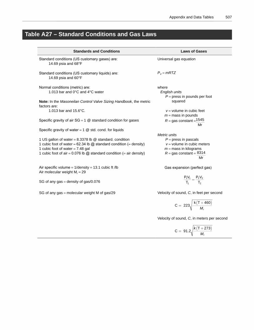
507Appendix and Data Tables
Table A27 – Standard Conditions and Gas Laws
Standards and Conditions Laws of Gases
Standard conditions (US customary gases) are:14.69 psia and 68°F
Standard conditions (US customary liquids) are:14.69 psia and 60°F
Normal conditions (metric) are:1.013 bar and 0°C and 4°C water
Note: In the Masoneilan Control Valve Sizing Handbook, the metric factors are:
1.013 bar and 15.6°C.
Specific gravity of air SG = 1 @ standard condition for gases
Specific gravity of water = 1 @ std. cond. for liquids
1 US gallon of water = 8.3378 lb @ standard. condition1 cubic foot of water = 62.34 lb @ standard condition (= density)1 cubic foot of water = 7.48 gal1 cubic foot of air = 0.076 lb @ standard condition (= air density)
Air specific volume = 1/density = 13.1 cubic ft /lbAir molecular weight Mr = 29
SG of any gas = density of gas/0.076
SG of any gas = molecular weight M of gas/29
Universal gas equation
PV = mRTZ
whereEnglish units
P = press in pounds per foot squared
v = volume in cubic feetm = mass in poundsR = gas constant =1545
Mr
Metric unitsP = press in pascalsv = volume in cubic meters
m = mass in kilogramsR = gas constant = 8314
Mr
Gas expansion (perfect gas)
P VT
P VT
1 1
1
2 2
2
=
Velocity of sound, C, in feet per second
C 223k T 460
=+( )Mr
Velocity of sound, C, in meters per second
C 91.2T 273
=+k
Mr
( )
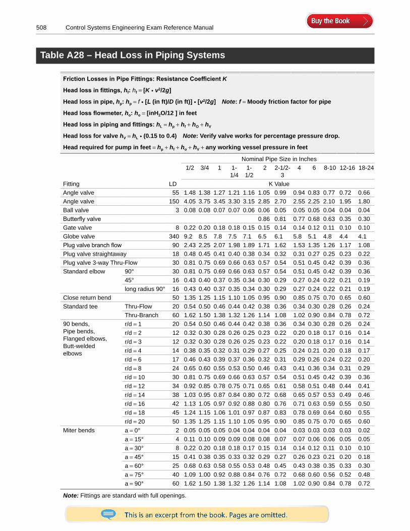
508 Control Systems Engineering Exam Reference Manual
Table A28 – Head Loss in Piping Systems
Friction Losses in Pipe Fittings: Resistance Coefficient K
Head loss in fittings, hf: hf = [K i v2/2g]
Head loss in pipe, hp: hp = f i [L (in ft)/D (in ft)] i [v2/2g] Note: f = Moody friction factor for pipe
Head loss flowmeter, ho: ho = [inH2O/12 ] in feet
Head loss in piping and fittings: hL = hp + hf + hO + hV
Head loss for valve hV = hL i (0 .15 to 0 .4) Note: Verify valve works for percentage pressure drop .
Head required for pump in feet = hp + hf + ho + hV + any working vessel pressure in feet
Fitting LD
Nominal Pipe Size in Inches1/2 3/4 1 1-
1/41- 1/2
2 2-1/2- 3
4 6 8-10 12-16 18-24
K ValueAngle valve 55 1.48 1.38 1.27 1.21 1.16 1.05 0.99 0.94 0.83 0.77 0.72 0.66Angle valve 150 4.05 3.75 3.45 3.30 3.15 2.85 2.70 2.55 2.25 2.10 1.95 1.80Ball valve 3 0.08 0.08 0.07 0.07 0.06 0.06 0.05 0.05 0.05 0.04 0.04 0.04Butterfly valve 0.86 0.81 0.77 0.68 0.63 0.35 0.30Gate valve 8 0.22 0.20 0.18 0.18 0.15 0.15 0.14 0.14 0.12 0.11 0.10 0.10Globe valve 340 9.2 8.5 7.8 7.5 7.1 6.5 6.1 5.8 5.1 4.8 4.4 4.1Plug valve branch flow 90 2.43 2.25 2.07 1.98 1.89 1.71 1.62 1.53 1.35 1.26 1.17 1.08Plug valve straightaway 18 0.48 0.45 0.41 0.40 0.38 0.34 0.32 0.31 0.27 0.25 0.23 0.22Plug valve 3-way Thru-Flow 30 0.81 0.75 0.69 0.66 0.63 0.57 0.54 0.51 0.45 0.42 0.39 0.36Standard elbow 90° 30 0.81 0.75 0.69 0.66 0.63 0.57 0.54 0.51 0.45 0.42 0.39 0.36
45° 16 0.43 0.40 0.37 0.35 0.34 0.30 0.29 0.27 0.24 0.22 0.21 0.19long radius 90° 16 0.43 0.40 0.37 0.35 0.34 0.30 0.29 0.27 0.24 0.22 0.21 0.19
Close return bend 50 1.35 1.25 1.15 1.10 1.05 0.95 0.90 0.85 0.75 0.70 0.65 0.60Standard tee Thru-Flow 20 0.54 0.50 0.46 0.44 0.42 0.38 0.36 0.34 0.30 0.28 0.26 0.24
Thru-Branch 60 1.62 1.50 1.38 1.32 1.26 1.14 1.08 1.02 0.90 0.84 0.78 0.7290 bends, Pipe bends, Flanged elbows, Butt-welded elbows
r/d = 1 20 0.54 0.50 0.46 0.44 0.42 0.38 0.36 0.34 0.30 0.28 0.26 0.24r/d = 2 12 0.32 0.30 0.28 0.26 0.25 0.23 0.22 0.20 0.18 0.17 0.16 0.14r/d = 3 12 0.32 0.30 0.28 0.26 0.25 0.23 0.22 0.20 0.18 0.17 0.16 0.14r/d = 4 14 0.38 0.35 0.32 0.31 0.29 0.27 0.25 0.24 0.21 0.20 0.18 0.17r/d = 6 17 0.46 0.43 0.39 0.37 0.36 0.32 0.31 0.29 0.26 0.24 0.22 0.20r/d = 8 24 0.65 0.60 0.55 0.53 0.50 0.46 0.43 0.41 0.36 0.34 0.31 0.29r/d = 10 30 0.81 0.75 0.69 0.66 0.63 0.57 0.54 0.51 0.45 0.42 0.39 0.36r/d = 12 34 0.92 0.85 0.78 0.75 0.71 0.65 0.61 0.58 0.51 0.48 0.44 0.41r/d = 14 38 1.03 0.95 0.87 0.84 0.80 0.72 0.68 0.65 0.57 0.53 0.49 0.46r/d = 16 42 1.13 1.05 0.97 0.92 0.88 0.80 0.76 0.71 0.63 0.59 0.55 0.50r/d = 18 45 1.24 1.15 1.06 1.01 0.97 0.87 0.83 0.78 0.69 0.64 0.60 0.55r/d = 20 50 1.35 1.25 1.15 1.10 1.05 0.95 0.90 0.85 0.75 0.70 0.65 0.60
Miter bends a = 0° 2 0.05 0.05 0.05 0.04 0.04 0.04 0.04 0.03 0.03 0.03 0.03 0.02a = 15° 4 0.11 0.10 0.09 0.09 0.08 0.08 0.07 0.07 0.06 0.06 0.05 0.05a = 30° 8 0.22 0.20 0.18 0.18 0.17 0.15 0.14 0.14 0.12 0.11 0.10 0.10a = 45° 15 0.41 0.38 0.35 0.33 0.32 0.29 0.27 0.26 0.23 0.21 0.20 0.18a = 60° 25 0.68 0.63 0.58 0.55 0.53 0.48 0.45 0.43 0.38 0.35 0.33 0.30a = 75° 40 1.09 1.00 0.92 0.88 0.84 0.76 0.72 0.68 0.60 0.56 0.52 0.48a = 90° 60 1.62 1.50 1.38 1.32 1.26 1.14 1.08 1.02 0.90 0.84 0.78 0.72
Note: Fittings are standard with full openings.