Standard Title Page - Report on State Project

Report No. Report Date No. Pages Type Report: Final Project No.: 70984

VTRC 05-CR22 June 2005 57 Period Covered:

10/01/03 to 4/30/05 Contract No.

Title: Laboratory Tests for Hot-Mix Asphalt Characterization in Virginia

Key Words: HMA Characterization, Resilient Modulus, Dynamic Modulus, Creep Compliance, Indirect Tensile Strength.

Authors:

Gerardo W. Flintsch, Ph.D., P.E., Imad L. Al-Qadi, Ph.D., P.E., Amara Loulizi, Ph.D., P.E., and David Mokarem, Ph.D.

Performing Organization Name and Address: Virginia Tech Transportation Institute 3500 Transportation Research Plaza Blacksburg, VA 24061

Sponsoring Agencies’ Name and Address Virginia Department of Transportation 1401 E. Broad Street Richmond, VA 23219

Supplementary Notes

Abstract: This project reviewed existing laboratory methods for accurately describing the constitutive behavior of the mixes used in the Commonwealth of Virginia. Indirect tensile (IDT) strength, resilient modulus, static creep in the IDT and uniaxial modes, flexural beam fatigue, and dynamic modulus tests were conducted on two typical mixes used in Virginia: SM-9.5A (surface mix) and BM-25.0 (base mix). The tests conducted produced a wealth of data on typical values for the properties of the two mixes studied over a wide range of temperatures and loading frequencies. The results suggest that the IDT strength test is an effective test to characterize the tensile strength of hot-mix asphalt (HMA), especially for thermal cracking evaluation. The resilient modulus test and the static creep test in the IDT setup are practical and simple to perform, but the analysis of the measurements is complicated, and the variability of the results is high. The compressive uniaxial dynamic modulus and the uniaxial static creep tests were found to be simple to conduct and to analyze because of the homogeneous state of stress in the specimen during testing. The flexural fatigue test was time consuming, but the test produces valuable information about the fatigue properties of hot-mix asphalt. The investigation also found good correlations among the IDT strength, resilient modulus, and dynamic modulus results. A variety of tests is recommended for characterizing the mechanistic-empirical pavement analysis and design. These tests would provide the properties needed to characterize the asphalt layers for the pavement analysis and design. The recommended tests are as follows: IDT strength for characterizing HMA susceptibility to thermal cracking, dynamic modulus for characterization of the constitutive behavior of the HMA, uniaxial creep for characterizing permanent deformation characteristics, and flexural fatigue tests to characterize fatigue properties. Materials characterization testing can be a valuable tool in pavement design. The use of mechanistic-empirical modeling can be used to predict the performance of a pavement. With this type of testing and modeling, the materials used in pavements will be of better quality and more resistant to environmental and structural deterioration. A more durable pavement will aid in reducing the frequency and costs associated with maintenance.

FINAL CONTRACT REPORT

LABORATORY TESTS FOR HOT-MIX ASPHALT CHARACTERIZATION IN VIRGINIA

Gerardo W. Flintsch, Ph.D., P.E. Roadway Infrastructure Group Leader, VTTI, Virginia Tech

Imad L. Al-Qadi, Ph.D., P.E. Founder's Professor of CEE, University of Illinois at Urbana-Champaign

Amara Loulizi, Ph.D., P.E. Research Scientist, VTTI, Virginia Tech

David Mokarem, Ph.D.

Research Scientist, Virginia Transportation Research Council

Project Manager David Mokarem, Ph.D., Virginia Transportation Research Council

Contract Research Sponsored by Virginia Transportation Research Council

Virginia Transportation Research Council (A Cooperative Organization Sponsored Jointly by the

Virginia Department of Transportation and the University of Virginia)

Charlottesville, Virginia

June 2005

VTRC 05-CR22

ii

NOTICE

The project that is the subject of this report was done under contract for the Virginia Department of Transportation, Virginia Transportation Research Council. The contents of this report reflect the views of the authors, who are responsible for the facts and the accuracy of the data presented herein. The contents do not necessarily reflect the official views or policies of the Virginia Department of Transportation, the Commonwealth Transportation Board, or the Federal Highway Administration. This report does not constitute a standard, specification, or regulation. Each contract report is peer reviewed and accepted for publication by Research Council staff with expertise in related technical areas. Final editing and proofreading of the report are performed by the contractor.

Copyright 2005 by the Commonwealth of Virginia.

iii

ABSTRACT

This project reviewed existing laboratory methods for accurately describing the constitutive behavior of the mixes used in the Commonwealth of Virginia. Indirect tensile (IDT) strength, resilient modulus, static creep in the IDT and uniaxial modes, flexural beam fatigue, and dynamic modulus tests were conducted on two typical mixes used in Virginia: SM-9.5A (surface mix) and BM-25.0 (base mix).

The tests conducted produced a wealth of data on typical values for the properties of the two mixes studied over a wide range of temperatures and loading frequencies. The results suggest that the IDT strength test is an effective test to characterize the tensile strength of hot-mix asphalt (HMA), especially for thermal cracking evaluation. The resilient modulus test and the static creep test in the IDT setup are practical and simple to perform, but the analysis of the measurements is complicated, and the variability of the results is high. The compressive uniaxial dynamic modulus and the uniaxial static creep tests were found to be simple to conduct and to analyze because of the homogeneous state of stress in the specimen during testing. The flexural fatigue test was time consuming, but the test produces valuable information about the fatigue properties of hot-mix asphalt. The investigation also found good correlations among the IDT strength, resilient modulus, and dynamic modulus results. A variety of tests is recommended for characterizing the mechanistic-empirical pavement analysis and design. These tests would provide the properties needed to characterize the asphalt layers for the pavement analysis and design. The recommended tests are as follows: IDT strength for characterizing HMA susceptibility to thermal cracking, dynamic modulus for characterization of the constitutive behavior of the HMA, uniaxial creep for characterizing permanent deformation characteristics, and flexural fatigue tests to characterize fatigue properties.

Materials characterization testing can be a valuable tool in pavement design. The use of mechanistic-empirical modeling can be used to predict the performance of a pavement. With this type of testing and modeling, the materials used in pavements will be of better quality and more resistant to environmental and structural deterioration. A more durable pavement will aid in reducing the frequency and costs associated with maintenance.

1

FINAL CONTRACT REPORT

LABORATORY TESTS FOR HOT-MIX ASPHALT CHARACTERIZATION IN VIRGINIA

Gerardo W. Flintsch, Ph.D., P.E. Roadway Infrastructure Group Leader, VTTI, Virginia Tech

Imad L. Al-Qadi, Ph.D., P.E. Founder's Professor of CEE, University of Illinois at Urbana-Champaign

Amara Loulizi, Ph.D., P.E. Research Scientist, VTTI, Virginia Tech

David Mokarem, Ph.D., Research Scientist Virginia Transportation Research Council

INTRODUCTION

With the current trend toward mechanistic flexible pavement design and the need for more reliable design procedures, accurate characterization of hot-mix asphalt (HMA) properties is vital. Over the years, several test methods were developed to characterize HMA. Until recently, the most accepted test method was the resilient modulus test. Several design methods, such as the 1993 American Association of State Highway and Transportation Officials (AASHTO) design guide, the Asphalt Institute design method, and the Australian pavement design guide, have all incorporated the modulus of resilience into the design process. However, in the proposed mechanistic-empirical (M-E) design guide developed by the recently completed National Cooperative Highway Research Programs (NCHRP) Project 1-37 A, this test has been replaced by the complex dynamic modulus to characterize HMA.

In addition, the simple performance tests as recommended by the NCHRP Project 9-19 require the use of different test setups to obtain the different HMA characterization parameters. For instance, the following tests are recommended:

�� To evaluate permanent deformation behavior: (1) dynamic modulus term, E*/sin �, obtained from the triaxial dynamic modulus test; (2) flow time, Ft, obtained from the triaxial static creep test; and (3) flow number, Fn, obtained from the triaxial repeated load test.

�� To evaluate fatigue cracking behavior: dynamic modulus measured at low temperatures.

�� To evaluate thermal cracking behavior: creep compliance measured by the indirect tensile creep test at long loading times and low temperatures.

Consequently, there is a need to evaluate existing procedures for characterizing HMA

and assess their practicality and the usefulness of the information provided for supporting M-E pavement design.

2

PURPOSE AND SCOPE

The objective of this research was to review existing methods for determining the moduli of HMA and to identify simple laboratory tests that accurately describe the constitutive behavior of HMA used in the Commonwealth of Virginia. The project considered several laboratory test methods, such as the modulus of resilience, creep compliance, flexural fatigue test, and dynamic modulus. Two HMA mixtures used in Virginia, SM-9.5 A and BM-25.0, were used to evaluate the various methods.

METHODS AND MATERIALS

This section discusses the procedures used through the investigation for preparing samples and for testing these samples according to the various methods evaluated. It also includes a short discussion of each of these methods.

Specimen Preparation and Volumetric Analysis All specimens were prepared according to typical job-mix formulas (JMF) provided by

the Virginia Transportation Research Council (VTRC), which are presented in Table 1. The needed aggregates, Reclaimed Asphalt Pavement (RAP) material, and asphalt binders were collected from suppliers. Batches of 15,000 g were prepared and stored in bags for future use. A total of 48 batches of SM-9.5A and 44 batches of BM-25.0 were prepared.

Table 1. Job mix formula for BM-25.0

Type Percentage (%) Source Location

BM-25.0 # 357 Limestone 18 ACCO STONE CO Blacksburg, VA #68 Limestone 30 ACCO STONE CO Blacksburg, VA #10 Limestone 27 ACCO STONE CO Blacksburg, VA Concrete Sand 10 WYTHE STONE CO Wytheville, VA Processed RAP 15 ADAMS CONSTRUCTION CO Blacksburg, VA

PG 64-22 4.7 ASSOCIATED ASPHALT CO Roanoke, VA Adhere HP+ 0.5 ARR-MAZ PRODUCTS Winter Haven, FL

SM-9.5A # 8 Quartzite 45 SALEM STONE CO Sylvatus, VA #10 Quartzite 25 SALEM STONE CO Sylvatus, VA Concrete Sand 15 WYTHE STONE CO Wytheville, VA Processed RAP 15 ADAMS CONSTRUCTION CO Blacksburg, VA

PG 64-22 5.5 ASSOCIATED ASPHALT CO Roanoke, VA Adhere HP+ 0.5 ARR-MAZ PRODUCTS Winter Haven, FL

The specimens for the IDT strength, resilient modulus test, static creep test, as well as the

ones used for the dynamic modulus test and uniaxial creep test, were prepared using a Troxler Gyratory compactor. Table 2 summarizes the molded specimen sizes and the final cut sizes for both mixes.

3

Table 2. Molded and final specimen sizes

SM-9.5A BM-25.0 Test Compacted size

mm (in) Final size mm (in)

Compacted size mm (in)

Final size mm (in)

150x115 (6x4) 150x75 (6x3) IDT strength

100x125 (4x5) 100x50 (4x2) 150x115 (6x4) 150x75 (6x3)

150x115 (6x4) 150x75 (6x3) Resilient Modulus (IDT)

100x125 (4x5) 100x50 (4x2) 150x115 (6x4) 150x75 (6x3)

Creep (IDT setup) 100x125 (4x5) 100x50 (4x2) 150x115 (6x4) 150x75 (6x3) Dynamic Modulus 150x178 (6x7) 100x150 (4x6) 150x178 (6x7) 100x150 (4x6)

Uniaxial Creep 150x178 (6x7) 100x150 (4x6) 150x178 (6x7) 100x150 (4x6) Fatigue Beam 432x64x50 (17x2.5x2) 432x64x50 (17x2.5x2)

The details of the sample preparation follow:

�� IDT specimens: All of the BM-25.0 specimens for the IDT strength, resilient modulus, and static creep tests were 150 mm (6 in) in diameter by approximately 115 mm (4.5 in) in thickness and were then cut to a final thickness of 75 mm (3 in). Two specimen sizes were used for the SM-9.5A mix. For this mix, specimens were prepared 150 mm (6 in) in diameter by 115 mm (4.5 in) in thickness and were cut to a final thickness of 75 mm (3 in); and 100 mm (4 in) in diameter by 125 mm (5 in) in thickness and cut to a final thickness of 50 mm (2 in). The IDT creep was performed only on the 100-mm (4-in) diameter specimens.

�� Dynamic modulus and uniaxial creep: 150-mm (6-in) diameter by 178-mm (7-in) thick specimens were prepared for both mixes, which were later cored and cut to a final size of 100 mm (4 in) in diameter by 150 mm (6 in) in thickness.

�� Beam fatigue: Specimens for the fatigue test were made using a PTI Asphalt Vibratory Compactor (AVC). The beam dimensions were 432 x 64 x 50 mm3 (17 x 2.5 x 2 in3).

Specific details regarding the number of specimens of each of the two mixes considered are

presented in the following sections.

SM-9.5A The first step was to find the right ingredient proportions to make a 15,000-g batch. The

asphalt content in the RAP material was determined by performing ignition tests on two RAP samples. The average asphalt content in the RAP material was approximately 5%. Therefore, the weights of all ingredients were calculated using this 5% value and according to the JMF.

The gradation of the mixed aggregates was then checked using representative samples from each aggregate and mixed according to the JMF. Three sieve analysis tests were performed according to the AASHTO T27 and T11. Table 3 presents the average results for the three performed tests, while Figure 1 shows the gradation curves for the three tests as well as the average values.

4

Table 3. Aggregate gradation for SM-9.5A mix

Sieve opening

(mm) Sieve # % Passing

Control Point LL

Control Point UL

Restricted Zone LL

Restricted Zone UL Decision

12.5 1/2 100.0 - 100 9.5 3/8 91.4 90 100 P

4.75 #4 56.3 90 2.36 #8 39.9 32 67 47.2 47.2 P 1.18 #16 31.2 - - 31.6 37.6 P 0.6 #30 23.1 - - 23.5 27.5 P 0.3 #50 14.2 - - 18.7 18.7 P

0.15 #100 9.7 - - 0.075 #200 7.4 2 10 P

12.59.54.752.381.180.60.30.0750

102030405060708090

100

Sieve Size Raised to 0.45 Power

Perc

ent P

assin

g

Gradation1Gradation2Gradation3Average

Figure 1. Aggregate gradation for SM-9.5A mix

The next step was to determine the maximum theoretical specific gravity (Gmm) of the

produced mix. The AASHTO T-209 procedure was followed on four samples produced from two different batches. The average value of Gmm was 2.467 (range = 2.459�2.479). This value was used in the calculation of the voids in total mix (VTM) for all the prepared specimens.

For the IDT strength test, resilient modulus, and static creep tests, the specimens were compacted using the Virginia Department of Transportation (VDOT) specified number of gyrations for the design of this type of mix, namely 65 gyrations. Six 150-mm diameter specimens and seven 100-mm diameter specimens were then tested to obtain their bulk density using the Corelok procedure (InstroTek, 2003).

5

Table 4 shows the results of the tests for both specimen sizes. The average Gmb of 2.377 was used to calculate the other volumetric properties; Table 5 summarizes the results.

Table 4. Corelok Gmb values for the standard SM-9.5A specimens

Size 100-mm 150-mm

2.379 2.382 2.374 2.386 2.375 2.361 2.373 2.374 2.378 2.384 2.375 2.382

Gmb

2.376 Average 2.376 2.378 Range 2.373-2.379 2.361-2.386

Table 5. Average volumetric properties for the Standard SM-9.5A specimens

Specification Property Average

value Minimum Maximum

Meet VDOT spec?

VTM (%) 3.6 2.5 5.5 P VMA (%) 14.9 15 P VFA (%) 76 68 84 P %Density 88.5 90.5 P F/A ratio 1.5 0.6 1.2 F

For the dynamic modulus and static uniaxial creep specimens, the weight needed to

produce a specimen 150 mm (6 in) in diameter and 178 mm (7 in) in thickness with 4% voids was calculated based on the measured Gmm value of 2.467. The number of gyrations was left variable to achieve the specified height of 178 mm (7 in). The bulk densities of the first three produced specimens were measured using the AASHTO T166 procedure, and the weight was adjusted to achieve 4% air voids based on these measurements. The Gmb of all produced specimens were measured using the AASHTO T166 procedure and are presented in Table 6 with the corresponding air void content.

A similar procedure was attempted for the fatigue beams. The weight needed to produce 4% voids in the beams was calculated based on the beam dimension. However, the AVC was not able to compact that quantity of material to the specified thickness of 50 mm (2 in). The weight was gradually decreased until the machine was able to compact the specimen to the specified thickness. AASHTO T166 procedure was then used to find the Gmb of the prepared beams and calculate their VTM (presented in Table 6).

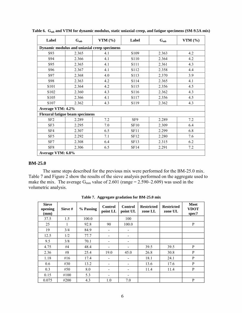
6

Table 6. Gmb and VTM for dynamic modulus, static uniaxial creep, and fatigue specimens (SM-9.5A mix)

Label Gmb VTM (%) Label Gmb VTM (%)

Dynamic modulus and uniaxial creep specimens S93 2.365 4.1 S109 2.363 4.2 S94 2.366 4.1 S110 2.364 4.2 S95 2.365 4.1 S111 2.361 4.3 S96 2.367 4.1 S112 2.358 4.4 S97 2.368 4.0 S113 2.370 3.9 S98 2.363 4.2 S114 2.365 4.1

S101 2.364 4.2 S115 2.356 4.5 S102 2.360 4.3 S116 2.362 4.3 S105 2.366 4.1 S117 2.356 4.5 S107 2.362 4.3 S119 2.362 4.3

Average VTM: 4.2% Flexural fatigue beam specimens

SF2 2.289 7.2 SF9 2.289 7.2 SF3 2.295 7.0 SF10 2.309 6.4 SF4 2.307 6.5 SF11 2.299 6.8 SF5 2.292 7.1 SF12 2.280 7.6 SF7 2.308 6.4 SF13 2.315 6.2 SF8 2.306 6.5 SF14 2.291 7.2

Average VTM: 6.8%

BM-25.0 The same steps described for the previous mix were performed for the BM-25.0 mix.

Table 7 and Figure 2 show the results of the sieve analysis performed on the aggregate used to make the mix. The average Gmm value of 2.601 (range = 2.590�2.609) was used in the volumetric analysis.

Table 7. Aggregate gradation for BM-25.0 mix

Sieve opening

(mm) Sieve # % Passing Control

point LL Control

point ULRestricted zone LL

Restricted zone UL

Meet VDOT spec?

37.5 1.5 100.0 100 25 1 92.8 90 100.0 P 19 3/4 84.9 - -

12.5 1/2 77.7 - - 9.5 3/8 70.1 - -

4.75 #4 48.4 - - 39.5 39.5 P 2.36 #8 25.4 19.0 45.0 26.8 30.8 P 1.18 #16 17.4 - - 18.1 24.1 P 0.6 #30 13.2 - - 13.6 17.6 P 0.3 #50 8.0 - - 11.4 11.4 P

0.15 #100 5.3 - - 0.075 #200 4.3 1.0 7.0 P

7

37.5251912.59.54.752.361.180.60.0750

102030405060708090

100

Sieve Size Raised to 0.45 Power

Perc

ent P

assin

g

Gradation 1Gradation2Gradation3Average

Figure 2. Aggregate gradation for BM-25.0 mix

The Corelok procedure was not used for measuring the Gmb of the BM-25 mix because

the rough edges of the specimens tore the plastic bags. Thus, the Gmb was measured according to AASHTO T166. The measured values were 2.430, 2.423, 2.447, 2.457, 2.458, and 2.428. The average value of 2.440 was used to determine the VTM.

Table 8 summarizes the calculated volumetric properties of the specimens prepared for the IDT strength, resilient modulus, and static creep tests. Even though the VTM specification was not met for this mix, it was decided that the samples were acceptable because the specimens were compacted to the required number of gyrations.

Table 8. Average volumetric properties for the standard BM-25.0 specimens

Specification Property Average

value Minimum Maximum

Meet VDOT spec?

VTM (%) 6.2 2.5 5.5 F VMA (%) 16.4 12 P VFA (%) 62.2 62 80 P %Density 86.1 89 P F/A ratio 1.0 0.6 1.3 P

For the dynamic modulus, uniaxial creep, and flexural fatigue specimens, the same procedure as described above for the SM-9.5A mix was repeated for the BM-25.0 mix. The volumetric properties for the compacted specimens are summarized in Table 9.

8

Table 9. Gmb and VTM for dynamic modulus and uniaxial creep specimens (BM-25.0 mix)

Label Gmb VTM (%) Label Gmb VTM (%)

Dynamic modulus and uniaxial creep specimens B55 2.464 5.2 B68 2.471 5.0 B56 2.473 4.9 B69 2.471 5.0 B58 2.467 5.1 B76 2.470 5.0 B60 2.463 5.3 B77 2.474 4.9 B61 2.474 4.9 B78 2.478 4.7 B62 2.473 4.9 B79 2.471 5.0 B63 2.470 5.0 B80 2.462 5.3 B64 2.473 4.9 B81 2.466 5.2 B65 2.465 5.2 B84 2.470 5.0 B67 2.473 4.9 B85 2.476 4.8

Average VTM: 5.0% Flexural fatigue beam specimens

BF1 2.374 8.7 BF8 2.346 9.8 BF2 2.403 7.6 BF9 2.328 10.5 BF3 2.379 8.5 BF10 2.342 9.9 BF4 2.381 8.4 BF11 2.333 10.3 BF6 2.323 10.7 BF12 2.338 10.1 BF7 2.345 9.8 BF13 2.354 9.5

Average VTM: 9.5%

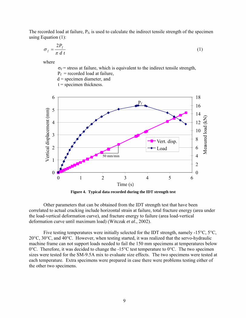
Indirect Tensile Strength Test The indirect tensile strength test is performed by loading a cylindrical specimen at a rate

of 50 mm/min along and parallel to its vertical diametral plane. This loading configuration develops a relatively uniform state of tensile stresses perpendicular to the load direction, which results in splitting of the specimen, as shown in Figure 3. During the test, load and vertical displacement are recorded as shown in Figure 4.

Figure 3. Specimen split after an IDT strength test

9

The recorded load at failure, Pf, is used to calculate the indirect tensile strength of the specimen using Equation (1):

tdPf

f�

�

2� (1)

where �f = stress at failure, which is equivalent to the indirect tensile strength, Pf = recorded load at failure, d = specimen diameter, and t = specimen thickness.

Figure 4. Typical data recorded during the IDT strength test

Other parameters that can be obtained from the IDT strength test that have been

correlated to actual cracking include horizontal strain at failure, total fracture energy (area under the load-vertical deformation curve), and fracture energy to failure (area load-vertical deformation curve until maximum load) (Witczak et al., 2002).

Five testing temperatures were initially selected for the IDT strength, namely -15°C, 5°C, 20°C, 30°C, and 40°C. However, when testing started, it was realized that the servo-hydraulic machine frame can not support loads needed to fail the 150 mm specimens at temperatures below 0°C. Therefore, it was decided to change the -15°C test temperature to 0°C. The two specimen sizes were tested for the SM-9.5A mix to evaluate size effects. The two specimens were tested at each temperature. Extra specimens were prepared in case there were problems testing either of the other two specimens.

10

Resilient Modulus Test (IDT Setup) This test has been traditionally used for determining the modulus of HMA specimens,

and ASTM adopted it as standard D4123 (ASTM, 1998). The test is relatively simple, and it has the advantage of being able to be used to test field cores. The test setup, shown in Figure 5, is similar to the one used in the IDT strength test, but the load used is dynamic. A pulse duration of 0.03 s followed by a rest period of 0.97 s was used in this study because it was found that this loading configuration best simulates the pulse load induced from moving trucks and from falling weight deflectometer (FWD) testing (Loulizi et al., 2002). The setup allows recording of the vertical and horizontal deformations at the center of the specimen that result from the applied pulse load.

Figure 5. Resilient modulus test configuration (IDT setup)

To obtain the resilient modulus value from the measured vertical and horizontal deformations, the Roque and Buttlar (1992) procedure was used. This procedure corrects for the effect of specimen bulging, which causes the externally mounted extensometers to rotate, resulting in errors in the vertical and horizontal deflection readings. Using this procedure, the resilient modulus (Mr) is computed using Equation (2):

xcorr

ycorrxcorrr

)(M

�

��� �

� (2)

where �xcorr = corrected horizontal point stress, �ycorr = corrected vertical point stress, � = Poisson�s ratio, and �xcorr = corrected horizontal strain.

The same five testing temperatures selected for the IDT test, -15°C, 5°C, 20°C, 30°C, and

40°C, were used for the resilient modulus test. Unlike the IDT strength test, testing at -15°C was possible because the specimen is loaded only to a strain level between 500 �m/m and 1,500 �m/m.

11

IDT Static Creep Compliance Test This test is run using the same configuration described for the IDT strength and resilient

modulus tests. The only difference is that a static load is applied for 1,000 s. The recorded horizontal and vertical deformations (Figure 6) are measured and used to calculate the creep compliance over time. Five different testing temperatures were used, -15°C, 5°C, 20°C, 30°C, and 40°C, and two specimens were tested at each temperature and size. Extra specimens were prepared to be used if necessary.

0

0.005

0.01

0.015

0.02

0.025

0 200 400 600 800 1000Time (s)

Def

orm

atio

n (m

m)

Vertical deformation 1Vertical deformation 2Horizontal deformation 1Horizontal deformation 2

Figure 6. Vertical and horizontal deformation over time during a static creep test in the IDT setup

The procedure developed by Kim et al. (2002) was used to calculate the creep

compliance over time from the measured vertical and horizontal deformations as follows in Equation (3):

� �)()()(D teVtcUPdt �� (3)

where D(t) = creep compliance at time t, d = specimen thickness, U(t) = measured horizontal deformation at time t, V(t) = measured vertical deformation at time t, and c and e = coefficients related to the specimen diameter and gauge length of the displacement measurements.

12

Fatigue Test (Flexural Beam Setup) The flexural beam fatigue test is performed by applying a sinusoidal load to a rectangular

beam. The third-point beam fatigue test applies loading at points located at one-third distances from the beam ends, as shown in Figure 7. This produces uniform bending in the central third of the specimen and significantly simplifies the analysis.

Figure 7. Third-point loading mode fatigue test apparatus

The general equations for analysis of a simply supported beam are presented in Equations (4), (5), and (6) (Huang, 1993):

2

3dbaP

t �� (4)

22 4312

aLd

t�

�

�� (5)

�3

22

4)43(

bdaLPaE �

� (6)

where σt = tensile stress, εt = tensile strain, δ = vertical deflection, P = applied load, L = beam span, a = distance between the load and the nearest support (L/3), b = beam width, d = beam depth, and E = stiffness modulus.

13

Fatigue testing was performed under a controlled-strain condition by applying a constant sinusoidal strain level at a frequency of 10 Hz and at ambient temperature (20°C). This means that the test results produced a relationship between applied strain and fatigue life, presented in Equation (7), which is commonly known as the Wöhler relationship.

n

F KN ���

����

��

0

1�

(7)

where NF = fatigue life (number of cycles to failure), K and n = mix-dependent constants, and εo = applied strain amplitude.

For this study, failure was defined as a 50% reduction in the specimen�s initial stiffness. The

specimen stiffness as a function of cycles is shown for a typical specimen in Figure 8. Four strain levels were used for characterizing the fatigue life of the two mixes evaluated. These levels were selected to provide a wide range of strain levels compatible with those developed in the pavement structure under typical traffic conditions. The defined strain levels were the following:

�� High strain level: applied strain above 500 �m/m,

�� Medium-high strain level: applied strain between 400 and 500 �m/m,

�� Medium-low strain level: applied strain between 300 and 400 �m/m), and

�� Low strain level: applied strain below 300 �m/m.

Figure 8. Stiffness versus number of cycles during a flexural fatigue test

14

As shown in Table 10, three beams were tested at each strain level. Therefore, 12 beams were tested per mix to establish their fatigue life response. Extra specimens were prepared for testing as necessary.

Table 10. Applied constant strain per tested beam

Strain (�m/m) Strain Level

BM-25.0 SM-9.5A 601 606 603 606 High Strain 551 548 487 487 488 490 Intermediate Strain 426 431 388 382 293 308 Medium Strain 318 332 248 253 205 194 Low Strain 221 221

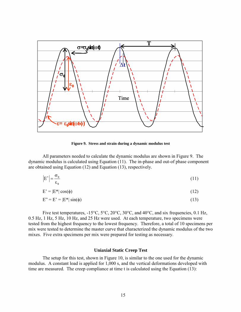
Dynamic Modulus Test (Uniaxial Setup) The dynamic modulus test, known also as the complex modulus test, is performed by

applying sinusoidal vertical loads to cylindrical specimens and measuring the corresponding vertical deformation. The test is usually performed at different temperatures and at different frequencies. The applied stress and corresponding measured strain are represented as follows in Equations (8) and (9):

� = �0 sin(�t) (8)

� = �0 sin(�t - �) (9)

where �0 = applied stress amplitude, �0 = measured strain amplitude, � = 2f = angular frequency, f = 1/T = frequency, T = period, and � = phase angle, computed as follows:

���� 360Tt∆ (10)

where t = time lag between the applied stress and the corresponding strain.

15

Time

�=�0sin(�t)

�= �0sin(�t-�)

�0

�0

T

�t

Time

�=�0sin(�t)

�= �0sin(�t-�)

�0

�0

T

�t

Figure 9. Stress and strain during a dynamic modulus test

All parameters needed to calculate the dynamic modulus are shown in Figure 9. The

dynamic modulus is calculated using Equation (11). The in-phase and out-of phase component are obtained using Equation (12) and Equation (13), respectively.

�

��

�

���� (11)

E� = |E*| cos(�) (12)

E� = E� = |E*| sin(�) (13)

Five test temperatures, -15°C, 5°C, 20°C, 30°C, and 40°C, and six frequencies, 0.1 Hz,

0.5 Hz, 1 Hz, 5 Hz, 10 Hz, and 25 Hz were used. At each temperature, two specimens were tested from the highest frequency to the lowest frequency. Therefore, a total of 10 specimens per mix were tested to determine the master curve that characterized the dynamic modulus of the two mixes. Five extra specimens per mix were prepared for testing as necessary.

Uniaxial Static Creep Test The setup for this test, shown in Figure 10, is similar to the one used for the dynamic

modulus. A constant load is applied for 1,000 s, and the vertical deformations developed with time are measured. The creep compliance at time t is calculated using the Equation (13):

16

� �

0

)(�

� ttD � (13)

where D(t) = creep compliance at time t, �(t) = measured vertical strain at time t, and �0 = applied constant stress.

The same five temperatures used for the dynamic modulus were used for this test: -15°C,

5°C, 20°C, 30°C, and 40°C. Two specimens per mix were tested at each temperature.

Figure 10. Creep compliance test in the uniaxial setup

17

RESULTS AND DISCUSSION

Indirect Tensile Strength Test

SM-9.5A Mix

Figure 11 shows the measured load versus the measured vertical deformation during testing for the 150-mm SM-9.5A specimens at all temperatures. As expected, the material stiffness increases, but becomes more brittle as the temperature decreases. This is shown by the increase in the required load to fail the specimen and by the decrease in the vertical displacement at failure as the temperature decreases. The same trend was found for the 100-mm specimens, but of course the load needed to break the specimens was smaller than that needed to fail the 150-mm specimens.

0102030405060708090

100

0 0.5 1 1.5 2 2.5 3 3.5 4 4.5 5 5.5

Displacement (mm)

Load

(kN

)

0°C

5°C

20°C

30°C

40°C

Figure 11. Load versus vertical deformation during IDT tests on SM-9.5A mix (150-mm specimens)

Table 11 presents a summary of the calculated IDT strength values as well as the fracture energy to failure for all tested specimens. The fracture energy to failure increases from 0ºC to 5ºC and then starts to decrease.

Figure 12 shows the calculated IDT strength versus temperature for both specimen sizes. In this figure, it can be seen that there is an inverse exponential relationship between IDT strength and temperature (in the temperature range of 5°C to 40°C). This is shown through the good fit of the data using the exponential equations (R2 as high as 0.98). However, the IDT strength seems to start to level off at temperatures below 5ºC, which means that the exponential equations should not be used to extrapolate the IDT strength below 0ºC. More testing is needed

18

to confirm the trend below 0ºC. There is also significant deformation in the proximity of the loading strip.

Table 11. Results of the IDT strength test for the SM-9.5A mix

Strength Average Strength Energy ID Temp.

(ºC) (kPa) (psi) (kPa) (psi) (Joules) (lb in)

150-mm specimens S19 0 4958 718.9 84.1 744.3 S22 0 5015 727.2

4987 723.1 84 743.5

S20 5 3760 545.2 91.4 809.0 S25 5 4195 608.3

3978 576.8 97.7 864.7

S21 20 1708 247.8 63.6 562.9 S30 20 1548 224.5

1628 236.2 57.2 506.3

S23 30 880 127.7 33.6 297.4 S26 30 756 109.6

818 118.6 28.5 252.2

S24 40 724 105.1 27.1 239.9 S29 40 583 84.6

654 94.8 24.5 216.8

100-mm specimens S31 0 4673 677.5 18.6 164.3 S38 0 5382 780.4

5028 728.9 25.4 224.8

S32 5 4404 638.6 25.8 228.3 S39 5 4562 661.5

4483 650.1 23.7 209.8

S33 20 1976 286.6 24.6 217.7 S40 20 2004 290.5

1990 288.5 21.5 190.3

S34 30 1051 152.4 13.2 116.8 S41 30 1152 167

1102 159.7 12.8 113.3

S35 40 492 71.9 4.6 40.7 S42 40 522 75.7

507 73.8 5.4 47.8

19

Strength = 5651.6e-0.0573T

R2 = 0.98

Strength = 4934.5e-0.0541T

R2 = 0.98

0

1000

2000

3000

4000

5000

6000

0 5 10 15 20 25 30 35 40

Temperature (°C)

Indi

rect

Ten

sile

Stre

ngth

(kPa

)100mm 150mm

Figure 12. IDT strength versus temperature for the SM-9.5A mix

Since the 100-mm and 150-mm specimens were both tested at the same deformation rate of 50 mm/min, it was expected that the strength of the 150-mm specimens would be smaller than that of the 100-mm specimens because of the lower strain rate.

As shown in Figure 13, on average, the IDT strength of the two tested sizes is similar at 0ºC, then the strength as obtained with the 100-mm diameter specimens becomes higher than that obtained with the 150-mm diameter specimens at temperatures of 5 ºC, 20 ºC, and 30ºC; the average ratio of the 100-mm diameter specimens� strength to that of the 150-mm diameter specimens is 1.1, 1.2, and 1.3 at temperatures of 5 ºC, 20 ºC, and 30 ºC, respectively.

However, at 40ºC the strength as obtained with the 150-mm diameter specimens is higher than that of the 100-mm diameter specimens with an average ratio of 1.3. This might be explained by the material testes in this IDT configuration could be less strain rate dependent at low temperatures. It has to be emphasized here that this test is mainly temperature dependent. Because of the high loading rates, the aggregate contribution becomes more significant at high temperatures.

20

0

1000

2000

3000

4000

5000

6000

0 5 20 30 40

Temperature (ºC)

IDT

stre

ngth

(kPa

)

150mm 100mm

Figure 13. Comparison between the IDT strength of 100-mm and 150-mm specimens

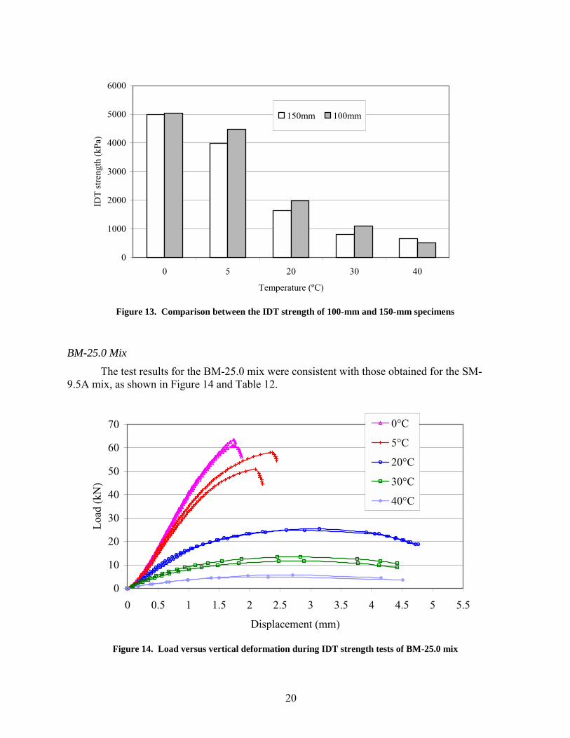
BM-25.0 Mix

The test results for the BM-25.0 mix were consistent with those obtained for the SM-9.5A mix, as shown in Figure 14 and Table 12.

0

10

20

30

40

50

60

70

0 0.5 1 1.5 2 2.5 3 3.5 4 4.5 5 5.5

Displacement (mm)

Load

(kN

)

0°C

5°C

20°C

30°C

40°C

Figure 14. Load versus vertical deformation during IDT strength tests of BM-25.0 mix

21

Table 12. Results of the IDT strength test for the BM-25.0 mix

Strength Average Strength Energy ID Temp (ºC) (kPa) (psi) (kPa) (psi) (Joules) (lb in)

B19 0 3369 488.5 56.2 497.4 B22 0 3540 513.3

3455 500.9 57.8 511.6

B20 5 2780 403.1 63.3 560.3 B25 5 3199 436.9

2990 420 84.7 749.7

B21 20 1371 198.8 50.5 447.0 B28 20 1403 203.5

1387 201.2 57.3 507.1

B23 30 646 93.6 24.4 216.0 B26 30 754 109.3

700 101.5 27.6 244.3

B24 40 316 45.9 10.5 92.9 B29 40 274 39.7

295 42.8 7.9 69.9

Figure 15 shows the IDT strength versus temperature for this mix. Again, the relationship between 0ºC and 40ºC could be modeled using an exponential equation. Like the SM-9.5A mix, leveling of the IDT strength around 5ºC is also noticeable from the figure.

Strength = 3941.6e-0.0609T

R2 = 0.98

0

500

1000

1500

2000

2500

3000

3500

4000

0 5 10 15 20 25 30 35 40Temperature (°C)

Indi

rect

Ten

sile

Stre

ngth

(kPa

)

Figure 15. IDT strength versus temperature for the BM-25.0 mix

Comparison

The IDT strengths at all testing temperatures for both mixes are compared in Figure 16. It is clear from this figure that the SM-9.5A mix shows higher tensile strength than the BM-25.0 mix. This is mainly attributed to the fact that the BM-25.0 mix has lower asphalt content and

22

higher air voids than the SM-9.5A mix. Figure 17 shows the average ratio of the SM-9.5A mix IDT strength to the BM-25.0 mix IDT strength. The ratio reaches a factor as high as 2.2 at a temperature of 40ºC.

A linear regression analysis using the SAS statistical package was used to verify whether the specimen size and the mix type have a statistically significant effect on the IDT strength. The data were analyzed as a completely randomized design (CRD) with effect type (SM-9.5A or BM-25.0), size within type (100 mm and 150 mm), temperature, and temperature squared as covariates. The interaction between size and mix type could not be differentiated because specimens were prepared in two sizes for only one of the mixes.

The IDT strength data were analyzed using the �mixed� procedure of SAS, using models with class variables type and width and with temperature as linear and quadratic terms as independent variables. As shown in Table 13, the temperature as a linear term, the temperature as quadratic term, and the mix type were very highly significant for IDT strength (p-values smaller than 0.05). The specimen size was found not to have a statistically significant effect (p-value greater than 0.05) on the test results.

0

1000

2000

3000

4000

5000

6000

0 5 20 30 40

Temperature (°C)

Indi

rect

Ten

sile

Stre

ngth

(kPa

) BM25.0SM9.5A

Figure 16. IDT strength comparison between SM-9.5A and BM-25.0 mixes

23

0

0.5

1

1.5

2

2.5

0 5 20 30 40

Temperature (ºC)

(ID

T st

reng

th S

M9.

5A)/(

IDT

Stre

ngth

B

M25

.0)

Figure 17. Ratio of the IDT strength of the SM-9.5A mix to the BM-25.0 mix

Table 13. Test of effects on the IDT strength

Effect F-value Pr > F Conclusion

Type 61.12 <0.0001 Significant Size (type) 3.08 0.0914 Not Significant

Temp. 164.14 <0.0001 Significant Temp*temp 9.69 0.0046 Significant

Resilient Modulus Test

SM-9.5A Mix

The same type of analysis used for the IDT strength was repeated for the resilient modulus data because the experimental program was similar for both tests. Table 14 shows the results for all the tested specimens.

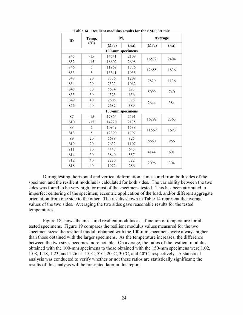
24

Table 14. Resilient modulus results for the SM-9.5A mix

Mr Average ID Temp.

(ºC) (MPa) (ksi) (MPa) (ksi) 100-mm specimens

S45 -15 14541 2109 S52 -15 18602 2698

16572 2404

S46 5 11969 1736 S53 5 13341 1935

12655 1836

S47 20 8336 1209 S54 20 7322 1062

7829 1136

S48 30 5674 823 S55 30 4523 656

5099 740

S49 40 2606 378 S56 40 2682 389

2644 384

150-mm specimens S7 -15 17864 2591

S10 -15 14720 2135 16292 2363

S8 5 10949 1588 S13 5 12390 1797

11669 1693

S9 20 5688 825 S19 20 7632 1107

6660 966

S11 30 4447 645 S14 30 3840 557

4144 601

S12 40 2220 322 S18 40 1972 286

2096 304

During testing, horizontal and vertical deformation is measured from both sides of the

specimen and the resilient modulus is calculated for both sides. The variability between the two sides was found to be very high for most of the specimens tested. This has been attributed to imperfect centering of the specimen, eccentric application of the load, and/or different aggregate orientation from one side to the other. The results shown in Table 14 represent the average values of the two sides. Averaging the two sides gave reasonable results for the tested temperatures.

Figure 18 shows the measured resilient modulus as a function of temperature for all tested specimens. Figure 19 compares the resilient modulus values measured for the two specimen sizes; the resilient moduli obtained with the 100-mm specimens were always higher than those obtained with the larger specimens. As the temperature increases, the difference between the two sizes becomes more notable. On average, the ratios of the resilient modulus obtained with the 100-mm specimens to those obtained with the 150-mm specimens were 1.02, 1.08, 1.18, 1.23, and 1.26 at -15°C, 5°C, 20°C, 30°C, and 40°C, respectively. A statistical analysis was conducted to verify whether or not these ratios are statistically significant; the results of this analysis will be presented later in this report.

25

y = -260.3x + 13125R2 = 0.95

y = -266.6x + 12437R2 = 0.97

02000400060008000

100001200014000160001800020000

-20 -15 -10 -5 0 5 10 15 20 25 30 35 40 45

Temperature (ºC)

Res

ilien

t Mod

ulus

(MPa

)100mm

150mm

Figure 18. Resilient modulus versus temperature for the SM-9.5A mix

0

2000

4000

6000

8000

10000

12000

14000

16000

18000

-15 5 20 30 40

Temperature (ºC)

Resi

lient

Mod

ulus

(MPa

)

150mm100mm

Figure 19. Comparison between the resilient modulus of 100-mm and 150-mm specimens

26

BM-25.0 Mix

Table 15 shows the resilient modulus measured for all the tested specimens. Figure 20 shows the measured resilient modulus as a function of temperature for all tested specimens.

Table 15. Resilient modulus results for the BM-25.0 mix

Mr Average ID Temp.

(ºC) (MPa) (ksi) (MPa) (ksi) B7 -15 15182 2202

B10 -15 18912 2743 17047 2473

B8 5 11852 1719 B13 5 10521 1526

11187 1623

B9 20 8556 1241 B16 20 6571 953

7564 1097

B11 30 4164 604 B14 30 4440 644

4302 624

B15 40 2565 372 B18 40 1986 288

2275 330

y = -270.82x + 12808R2 = 0.96

0

2000

4000

6000

8000

10000

12000

14000

16000

18000

20000

-20 -15 -10 -5 0 5 10 15 20 25 30 35 40 45

Temperature (ºC)

Res

ilien

t mod

ulus

(MPa

)

Figure 20. Resilient modulus versus temperature for the BM-25.0 mix

Comparison

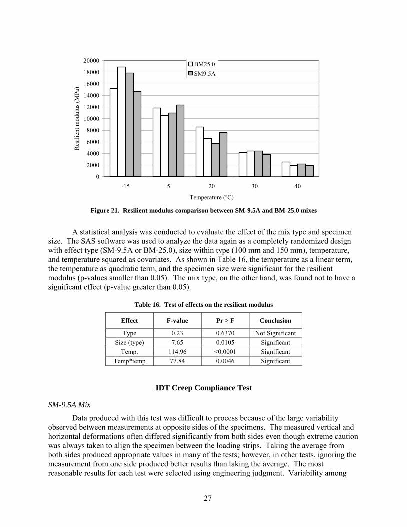
The resilient modulus of the SM-9.5A mix and the BM-25.0 mix measured on the 150-mm specimens are compared in Figure 21. In this case, it can be observed that the variation within the same mix samples (at the same temperature) is high. Furthermore, no clear trend in the relationship between the two mixes was noted.

27

0

2000

4000

6000

8000

10000

12000

14000

16000

18000

20000

-15 5 20 30 40

Temperature (ºC)

Res

ilien

t mod

ulus

(MPa

)

BM25.0SM9.5A

Figure 21. Resilient modulus comparison between SM-9.5A and BM-25.0 mixes

A statistical analysis was conducted to evaluate the effect of the mix type and specimen

size. The SAS software was used to analyze the data again as a completely randomized design with effect type (SM-9.5A or BM-25.0), size within type (100 mm and 150 mm), temperature, and temperature squared as covariates. As shown in Table 16, the temperature as a linear term, the temperature as quadratic term, and the specimen size were significant for the resilient modulus (p-values smaller than 0.05). The mix type, on the other hand, was found not to have a significant effect (p-value greater than 0.05).

Table 16. Test of effects on the resilient modulus

Effect F-value Pr > F Conclusion

Type 0.23 0.6370 Not Significant Size (type) 7.65 0.0105 Significant

Temp. 114.96 <0.0001 Significant Temp*temp 77.84 0.0046 Significant

IDT Creep Compliance Test

SM-9.5A Mix

Data produced with this test was difficult to process because of the large variability observed between measurements at opposite sides of the specimens. The measured vertical and horizontal deformations often differed significantly from both sides even though extreme caution was always taken to align the specimen between the loading strips. Taking the average from both sides produced appropriate values in many of the tests; however, in other tests, ignoring the measurement from one side produced better results than taking the average. The most reasonable results for each test were selected using engineering judgment. Variability among

28

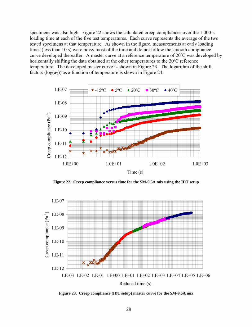
specimens was also high. Figure 22 shows the calculated creep compliances over the 1,000-s loading time at each of the five test temperatures. Each curve represents the average of the two tested specimens at that temperature. As shown in the figure, measurements at early loading times (less than 10 s) were noisy most of the time and do not follow the smooth compliance curve developed thereafter. A master curve at a reference temperature of 20ºC was developed by horizontally shifting the data obtained at the other temperatures to the 20ºC reference temperature. The developed master curve is shown in Figure 23. The logarithm of the shift factors (log(aT)) as a function of temperature is shown in Figure 24.

1.E-12

1.E-11

1.E-10

1.E-09

1.E-08

1.E-07

1.0E+00 1.0E+01 1.0E+02 1.0E+03

Time (s)

Cre

ep c

ompl

ianc

e (P

a-1)

-15ºC 5ºC 20ºC 30ºC 40ºC

Figure 22. Creep compliance versus time for the SM-9.5A mix using the IDT setup

1.E-12

1.E-11

1.E-10

1.E-09

1.E-08

1.E-07

1.E-03 1.E-02 1.E-01 1.E+00 1.E+01 1.E+02 1.E+03 1.E+04 1.E+05 1.E+06

Reduced time (s)

Cre

ep c

ompl

ianc

e (P

a-1)

Figure 23. Creep compliance (IDT setup) master curve for the SM-9.5A mix

29

y = -0.0707x + 1.0838R2 = 0.95

-4

-2

0

2

4

-20 -10 0 10 20 30 40 50Temperature (ºC)

log

(aT)

Figure 24. Shift factor versus temperature for the SM-9.5A mix (creep IDT setup)

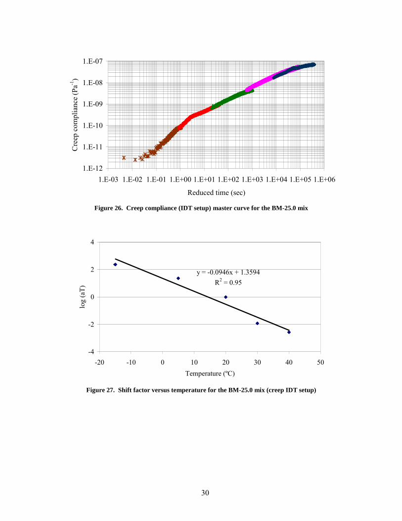
BM-25.0 Mix

The same types of problems noted for the SM-9.5A mix were encountered during testing of the BM-25.0 mix. Results for this mix are shown in Figure 25 through Figure 27. The comparison between the two mixes is presented later in this report after presenting the data obtained from the uniaxial creep test.

1.E-12

1.E-11

1.E-10

1.E-09

1.E-08

1.E-07

1.0E+00 1.0E+01 1.0E+02 1.0E+03

Time (s)

Cre

ep C

ompl

ianc

e (P

a-1)

-15ºC 5ºC 20ºC 30ºC 40ºC

Figure 25. Creep compliance versus time for the BM-25.0 mix using the IDT setup

30

1.E-12

1.E-11

1.E-10

1.E-09

1.E-08

1.E-07

1.E-03 1.E-02 1.E-01 1.E+00 1.E+01 1.E+02 1.E+03 1.E+04 1.E+05 1.E+06

Reduced time (sec)

Cre

ep c

ompl

ianc

e (P

a-1)

Figure 26. Creep compliance (IDT setup) master curve for the BM-25.0 mix

y = -0.0946x + 1.3594R2 = 0.95

-4

-2

0

2

4

-20 -10 0 10 20 30 40 50Temperature (ºC)

log

(aT)

Figure 27. Shift factor versus temperature for the BM-25.0 mix (creep IDT setup)

31

Fatigue Test (Flexural Beam Setup) The fatigue life at each strain level was plotted for each mix as shown in Figure 28. Once

all the points were plotted, a power regression equation was used to fit the data. It was found that the fatigue life of the SM-9.5A and BM-25.0 mixes are represented by Equations (14) and (15), respectively.

678.4

0

116586.3�

���

����

��

�

ENF (14)

683.3

0

113805.4�

���

����

��

�

EN F (15)

where NF = number of cycles to failure, and � �0 = applied stain amplitude.

These results suggest that the SM-9.5A mix has a longer fatigue life than the BM-25.0 in

the strain range applied within this testing (200 �m/m to 600 �m/m), which are typical strains the HMA layer may encounter during the pavement life. It must be noted that the two mixes had different binder contents and air voids.

y = 3.586E+16x-4.678

R2 = 0.97

y = 4.805E+13x-3.6833

R2 = 0.93

1000

10000

100000

1000000

100 1000Strain (�m/m)

Nf

BM25.0 SM-9.5A

Figure 28. Fatigue life for both mixes

32

Dynamic Modulus Test (Uniaxial Setup)

SM-9.5A Mix

Figure 29 shows the measured dynamic modulus results for the SM-9.5A mix as a function of frequency for each testing temperature. As expected, under a constant loading frequency, the magnitude of the dynamic modulus decreases with an increase in temperature; under a constant testing temperature, the magnitude of the dynamic modulus increases with an increase in the frequency.

100

1000

10000

100000

0.01 0.1 1 10 100Frequency (Hz)

|E*|

(MPa

)

-15°C 5°C 20°C 30°C 40°C

Figure 29. Dynamic modulus results for the SM-9.5A mix

Figure 30 shows the calculated phase angle results for all performed tests for the SM-

9.5A mix. From this figure it can be seen that the phase angle decreases as the frequency increases at testing temperatures of -15°C, 5°C, and 20°C. However, at testing temperatures of 30°C and 40°C, the behavior of the phase angle as a function of frequency is more complex.

At 30°C, the phase angle seems to increase up to frequencies of 0.5 Hz, and then it starts to decrease with an increase in frequency. At 40°C, the behavior of the phase angle with frequency is even more complex. At this temperature, the phase angle seems to increase from 0.1 Hz to 0.5 Hz, then it starts to decrease from 0.5 Hz to 1 Hz, and then it starts to increase again with frequency. At constant high frequencies (1 Hz to 25 Hz), the phase angle increases with an increase in temperature; at lower frequencies, the behavior of the phase angle with temperature is more complex.

The variation of the phase angle with frequency and temperature is qualitatively presented in Figure 31. The complex behavior of the phase angle at higher temperatures or at

33

lower frequencies is mainly attributed to aggregate interlock effects, as well as a networking of the binder at that temperature-frequency combination range.

0.1

1

10

100

0.01 0.1 1 10 100Frequency (Hz)

Phas

e an

gle

(°)

-15°C 5°C 20°C 30°C 40°C

Figure 30. Phase angle results for the SM-9.5A mix

25 10 5 1 0.5 0.1

-15

52030

40

0

5

10

15

20

25

30

35

Phas

e an

gle

(°)

Frequency (Hz)Temperature (°C)

-155203040

Figure 31. Average phase angle variation with temperature and frequency for the SM-9.5A mix

34

Figure 32 and Figure 33 show the variation of the average real and imaginary parts of the dynamic modulus, respectively, as a function of frequency at each testing temperature. The real part increases with a decrease in temperature or an increase in frequency. On the other hand, the imaginary part decreases with a frequency increase at low testing temperatures (-15°C and 5°C). At high temperatures (20°C to 40°C), the imaginary part increases with an increase in frequency.

100

1000

10000

100000

0.01 0.1 1 10 100Frequency (Hz)

E' (M

Pa)

-15°C 5°C 20°C 30°C 40°C

Figure 32. Real part of the dynamic modulus for the SM-9.5A mix

100

1000

10000

0.01 0.1 1 10 100Frequency (Hz)

E" (M

Pa)

-15°C 5°C 20°C 30°C 40°C

Figure 33. Imaginary part of the dynamic modulus for the SM-9.5A mix

35

Table 17 shows the average dynamic modulus for the SM-9.5A mix measured at each temperature and frequency. Table 18 shows the average calculated phase angle for the SM-9.5A mix at all temperatures and frequencies.

Table 17. Average dynamic modulus of the SM-9.5A mix in MPa (ksi)

Temperature (°C) -15 5 20 30 40

25 19563 (2837) 13833 (2006) 11312 (1641) 6722 (975) 3484 (505) 10 19117 (2773) 12058 (1749) 9787 (1419) 5432 (788) 2521 (366) 5 18750 (2719) 11313 (1641) 8609 (1249) 4384 (636) 1985 (288) 1 18285 (2652) 10118 (1468) 5953 (863) 2635 (382) 1226 (178)

0.5 17528 (2542) 8804 (1277) 4734 (687) 2054 (298) 709 (103)

Freq

uenc

y (H

z)

0.1 15940 (2312) 7432 (1078) 2890 (419) 1316 (191) 532 (77)

Table 18. Average phase angle results (in °) for the SM-9.5A mix

Temperature (°C)

-15 5 20 30 40 25 1.2 6.0 15.1 24.3 32.1 10 2.4 7.9 17.3 25.2 29.8 5 3.0 8.7 19.2 27.1 28.6 1 3.4 10.9 24.2 28.8 23.9

0.5 3.7 12.8 29.8 31.5 28.3

Freq

uenc

y (H

z)

0.1 5.1 16.3 33.4 28.2 19.6

A master curve of the dynamic modulus at the reference temperature of 20°C was constructed to complete the characterization of the material. The method developed by Pellinen and Witczak (2002) was used in this study to construct the master curve. The method consists of fitting a sigmoidal curve to the measured dynamic modulus test data using nonlinear least square regression techniques. The shift factors at each temperature are determined simultaneously with the other coefficients of the sigmoidal function. The function is given by Equation (16):

rfeE log

*

1log

��

��

�

�

�� (16)

where � �, �, �, and � = sigmoidal function coefficients (fit parameters), and fr = reduced frequency, which is given by the following equation:

Tr aff logloglog �� (17)

aT = shift factor at temperature T. The statistical software package SAS was used for the nonlinear regression analysis. The

determined coefficients for the SM-9.5A mix are shown in Table 19. The best fit master curve is presented in Figure 34. Figure 35 shows the variation of the shift factor with temperature.

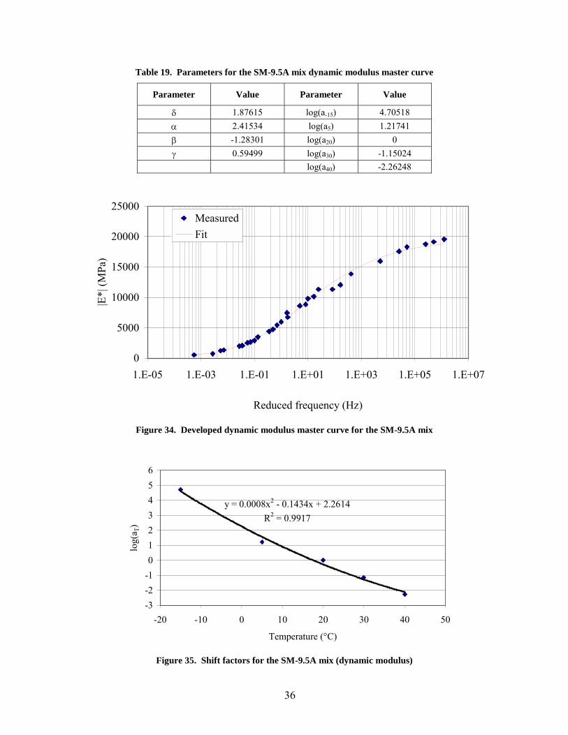
36

Table 19. Parameters for the SM-9.5A mix dynamic modulus master curve

Parameter Value Parameter Value

�� 1.87615 log(a-15) 4.70518 �� 2.41534 log(a5) 1.21741 �� -1.28301 log(a20) 0 �� 0.59499 log(a30) -1.15024 log(a40) -2.26248

0

5000

10000

15000

20000

25000

1.E-05 1.E-03 1.E-01 1.E+01 1.E+03 1.E+05 1.E+07

Reduced frequency (Hz)

|E*|

(MPa

)

MeasuredFit

Figure 34. Developed dynamic modulus master curve for the SM-9.5A mix

y = 0.0008x2 - 0.1434x + 2.2614R2 = 0.9917

-3-2-10123456

-20 -10 0 10 20 30 40 50

Temperature (°C)

log(

a T)

Figure 35. Shift factors for the SM-9.5A mix (dynamic modulus)

37

BM-25.0 Mix

Similar analysis to that of the SM-9.5A mix was performed on the BM-25.0 mix. Figure 36 and Figure 37 present the magnitude of the dynamic modulus and calculated phase angle, respectively, for the BM-25.0 mix as a function of frequency for each testing temperature.

100

1000

10000

100000

0.01 0.1 1 10 100Frequency (Hz)

|E*|

(MPa

)

-15°C 5°C 20°C 30°C 40°C

Figure 36. Dynamic modulus results for the BM-25.0 mix

1

10

100

0.01 0.1 1 10 100Frequency (Hz)

Phas

e an

gle

(°)

-15°C 5°C 20°C 30°C 40°C

Figure 37. Phase angle results for the BM-25.0 mix

38

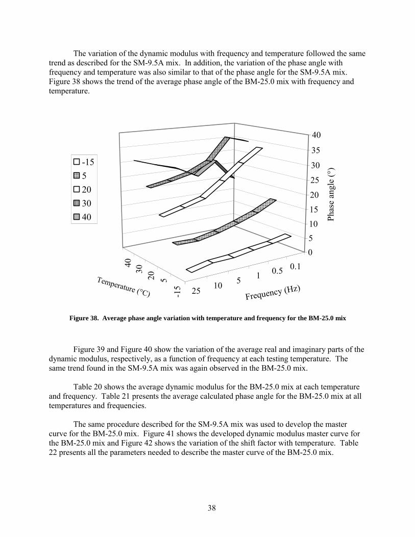
The variation of the dynamic modulus with frequency and temperature followed the same trend as described for the SM-9.5A mix. In addition, the variation of the phase angle with frequency and temperature was also similar to that of the phase angle for the SM-9.5A mix. Figure 38 shows the trend of the average phase angle of the BM-25.0 mix with frequency and temperature.

25 10 5 1 0.5 0.1

-15

52030

40

051015

20

25

30

35

40

Phas

e an

gle

(°)

Frequency (Hz)Temperature (°C)

-155203040

Figure 38. Average phase angle variation with temperature and frequency for the BM-25.0 mix

Figure 39 and Figure 40 show the variation of the average real and imaginary parts of the dynamic modulus, respectively, as a function of frequency at each testing temperature. The same trend found in the SM-9.5A mix was again observed in the BM-25.0 mix.

Table 20 shows the average dynamic modulus for the BM-25.0 mix at each temperature

and frequency. Table 21 presents the average calculated phase angle for the BM-25.0 mix at all temperatures and frequencies.

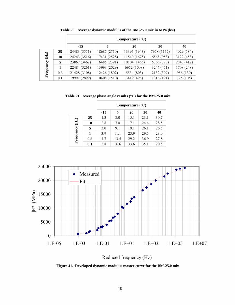
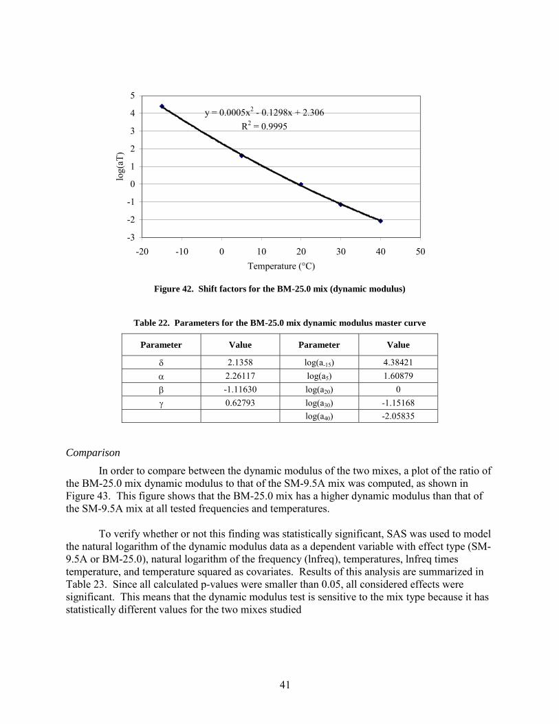
The same procedure described for the SM-9.5A mix was used to develop the master curve for the BM-25.0 mix. Figure 41 shows the developed dynamic modulus master curve for the BM-25.0 mix and Figure 42 shows the variation of the shift factor with temperature. Table 22 presents all the parameters needed to describe the master curve of the BM-25.0 mix.

39

100

1000

10000

100000

0.01 0.1 1 10 100Frequency (Hz)

E' (M

Pa)

-15°C 5°C 20°C 30°C 40°C

Figure 39. Real part of the dynamic modulus for the BM-25.0 mix

100

1000

10000

0.01 0.1 1 10 100Frequency (Hz)

E" (M

Pa)

-15°C 5°C 20°C 30°C 40°C

Figure 40. Imaginary part of the dynamic modulus for the BM-25.0 mix

40

Table 20. Average dynamic modulus of the BM-25.0 mix in MPa (ksi)

Temperature (°C)

-15 5 20 30 40 25 24483 (3551) 18687 (2710) 13395 (1943) 7978 (1157) 4029 (584) 10 24243 (3516) 17431 (2528) 11549 (1675) 6568 (953) 3122 (453) 5 23867 (3462) 16485 (2391) 10104 (1465) 5366 (778) 2843 (412) 1 22484 (3261) 13993 (2029) 6952 (1008) 3246 (471) 1708 (248)

0.5 21428 (3108) 12426 (1802) 5534 (803) 2132 (309) 956 (139)

Freq

uenc

y (H

z)

0.1 19991 (2899) 10408 (1510) 3419 (496) 1316 (191) 725 (105)

Table 21. Average phase angle results (°C) for the BM-25.0 mix

Temperature (°C)

-15 5 20 30 40 25 1.3 8.0 15.1 23.1 30.7 10 2.8 7.8 17.1 24.4 28.5 5 3.0 9.1 19.1 26.1 26.5 1 3.9 11.1 23.9 29.5 23.0

0.5 4.7 13.5 29.2 36.9 27.8

Freq

uenc

y (H

z)

0.1 5.8 16.6 33.6 35.1 20.5

0

5000

10000

15000

20000

25000

1.E-05 1.E-03 1.E-01 1.E+01 1.E+03 1.E+05 1.E+07

Reduced frequency (Hz)

|E*|

(MPa

)

MeasuredFit

Figure 41. Developed dynamic modulus master curve for the BM-25.0 mix

41

y = 0.0005x2 - 0.1298x + 2.306R2 = 0.9995

-3

-2

-1

0

1

2

3

4

5

-20 -10 0 10 20 30 40 50Temperature (°C)

log(

aT)

Figure 42. Shift factors for the BM-25.0 mix (dynamic modulus)

Table 22. Parameters for the BM-25.0 mix dynamic modulus master curve

Parameter Value Parameter Value

�� 2.1358 log(a-15) 4.38421 �� 2.26117 log(a5) 1.60879 �� -1.11630 log(a20) 0 �� 0.62793 log(a30) -1.15168 log(a40) -2.05835

Comparison

In order to compare between the dynamic modulus of the two mixes, a plot of the ratio of the BM-25.0 mix dynamic modulus to that of the SM-9.5A mix was computed, as shown in Figure 43. This figure shows that the BM-25.0 mix has a higher dynamic modulus than that of the SM-9.5A mix at all tested frequencies and temperatures.

To verify whether or not this finding was statistically significant, SAS was used to model the natural logarithm of the dynamic modulus data as a dependent variable with effect type (SM-9.5A or BM-25.0), natural logarithm of the frequency (lnfreq), temperatures, lnfreq times temperature, and temperature squared as covariates. Results of this analysis are summarized in Table 23. Since all calculated p-values were smaller than 0.05, all considered effects were significant. This means that the dynamic modulus test is sensitive to the mix type because it has statistically different values for the two mixes studied

42

0

0.2

0.4

0.6

0.8

1

1.2

1.4

1.6

0.1 0.5 1 5 10 25

Frequency (Hz)

|E*|

BM

25.5

/ |E

*|SM

-9.5

A-15°C 5°C 20°C 30°C 40°C

Figure 43. Ratio between BM-25.0 mix dynamic modulus to that of the SM-9.5A mix

Table 23. Test of effects on dynamic modulus

Effect F-Value p-value

Mix 77.57 < 0.0001 lnfreq 162.29 < 0.0001 temp 702.29 < 0.0001

lnfreq*temp 291.86 < 0.0001 Tem*temp 283.43 < 0.0001

Uniaxial Static Creep Compliance Test

SM-9.5A Mix

Figure 44 shows calculated creep compliances over the 1,000-s loading time at each of the five tested temperatures. Each curve represents the average of the two tested specimens at that temperature. Measurements at early loading times (less than 10 s) were not as noisy as those obtained with the IDT setup. The master curve at a reference temperature of 20ºC, developed as described for the IDT setup, is presented in Figure 45. Figure 46 shows a plot of the logarithm of the shift factors (log(aT)) as a function of temperature.

43

1.0E-10

1.0E-09

1.0E-08

1.0E-07

1.0E+00 1.0E+01 1.0E+02 1.0E+03

Time (s)

Cre

ep c

ompl

ianc

e (P

a-1)

-15°C 5°C 20°C 30°C 40°C

Figure 44. Creep compliance versus time for the SM-9.5A mix using the uniaxial setup

1.E-10

1.E-09

1.E-08

1.E-07

1.E-03 1.E-02 1.E-01 1.E+00 1.E+01 1.E+02 1.E+03 1.E+04 1.E+05

Reduced time (s)

Cre

ep c

ompl

ianc

e (P

a-1)

Figure 45. Creep compliance (uniaxial setup) master curve for the SM-9.5A mix

44

y = -0.0793x + 1.3872R2 = 0.99

-6

-3

0

3

6

-20 -10 0 10 20 30 40 50Temperature (°C)

log(

a T)

Figure 46. Shift factor versus temperature for the SM-9.5A mix (creep uniaxial setup)

BM-25.0 Mix

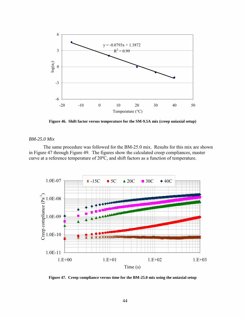
The same procedure was followed for the BM-25.0 mix. Results for this mix are shown in Figure 47 through Figure 49. The figures show the calculated creep compliances, master curve at a reference temperature of 20ºC, and shift factors as a function of temperature.

1.0E-11

1.0E-10

1.0E-09

1.0E-08

1.0E-07

1.E+00 1.E+01 1.E+02 1.E+03Time (s)

Cre

ep c

ompl

ianc

e (P

a-1)

-15C 5C 20C 30C 40C

Figure 47. Creep compliance versus time for the BM-25.0 mix using the uniaxial setup

45

1.E-11

1.E-10

1.E-09

1.E-08

1.E-07

1.E-04 1.E-03 1.E-02 1.E-01 1.E+00 1.E+01 1.E+02 1.E+03 1.E+04 1.E+05Reduced time (s)

Cre

ep c

ompl

ianc

e (P

a-1)

Figure 48. Creep compliance (uniaxial setup) master curve for the BM-25.0 mix

y = -0.1091x + 2.3588R2 = 0.99

-6

-3

0

3

6

-20 -10 0 10 20 30 40 50Temperature (°C)

log(

a T)

Figure 49. Shift factor versus temperature for the BM-25.0 mix (creep uniaxial setup)

Comparison

Table 24 compares the results for the creep compliance at selected loading times for both mixes using the IDT and uniaxial setups. From this table, it is noted that using the IDT setup, the creep compliance of the BM-25.0 mix is lower than that of the SM-9.5A mix at all loading times.

46

On the other hand, using the uniaxial setup, the creep compliance of the BM-25.0 is lower than that of the SM-9.5A mix only at loading times of 1 s to 10 s. At longer loading times (more than 100 s), the creep compliance of the SM-9.5A mix becomes slightly lower than that of the BM-25.0.

Table 24. Comparison between creep compliances [in Pa-1 (psi-1)] at 20ºC for both mixes using both setups

IDT setup Uniaxial setup Time (s)

SM-9.5A BM-25.0 SM-9.5A BM-25.0 1 3.30E-11 (2.28E-07) 1.00E-10 (6.89E-07) 5.80E-10 (4.00E-06) 3.80E-10 (2.62E-06)

10 3.60E-10 (2.48E-06) 4.50E-10 (3.10E-06) 1.24E-09 (8.55E-06) 1.22E-09 (8.41E-06) 100 1.20E-09 (8.27E-06) 1.70E-09 (1.17E-05) 2.98E-09 (2.05E-05) 3.10E-09 (2.14E-05)

1000 3.00E-09 (2.07E-05) 6.30E-09 (4.34E-05) 5.90E-09 (4.07E-05) 7.00E-09 (4.83E-05) 10000 7.00E-09 (4.83E-05) 2.10E-08 (1.45E-04) 9.60E-09 (6.62E-05) 1.23E-08 (8.48E-05)

If it is assumed that the relaxation modulus is equal to the inverse of the creep

compliance, which is a rough estimate but only used here for comparison purposes, then the SM-9.5A would have a very high modulus at all loading times but especially at lower ones, as shown in Table 25. For the BM-25.0 mix, the values are also high at lower loading times but are more reasonable at long loading times. These problems could be due to either the difficulties encountered in measuring the vertical and horizontal deformation in the IDT setup or to the method used to calculate the creep compliance in the IDT setup. In fact, in the IDT setup, a multiaxial state of stress exists in the specimen upon loading, which makes the interpretation of the test results difficult. On the other hand, results obtained using the uniaxial setup were more realistic, as shown in Table 25. In this setup, the state of stress in the specimen is much simpler than that in the IDT setup, making the results easier to interpret.

Table 25. Approximate relaxation moduli at 20ºC for both mixes [in MPa (ksi)] using both setups

IDT Setup Uniaxial Time

SM-9.5A BM-25.0 SM-9.5A BM-25.0 1 3.03E+04 (4395) 1.00E+04 (1450) 1.72E+03 (250) 2.63E+03 (382)

10 2.78E+03 (403) 2.22E+03 (322) 8.06E+02 (117) 8.20E+02 (119) 100 8.33E+02 (121) 5.88E+02 (85) 3.36E+02 (49) 3.23E+02 (47)

1000 3.33E+02 (48) 1.59E+02 (23) 1.69E+02 (25) 1.43E+02 (21) 10000 1.43E+02 (21) 4.76E+01 (7) 1.04E+02 (15) 8.13E+01 (12)

Correlation between Resilient Modulus and IDT Strength Figure 50 shows a plot of the average resilient modulus results versus the average IDT

strength results per mix and per specimen size. From this figure, it is clear that there is a strong correlation between the resilient modulus and the IDT strength. However, the correlation is mix dependent. For the BM-25.0 mix, the resilient modulus in MPa is equal to almost 4.56 times the

47

IDT strength in kPa. For the SM-9.5A mix, the resilient modulus in MPa is almost equal to 3.2 times the IDT strength in kPa.

y = 4.56xR2 = 0.92

y = 3.22xR2 = 0.96

y = 3.20xR2 = 0.93

0

2000

4000

6000

8000

10000

12000

14000

16000

18000

0 1000 2000 3000 4000 5000 6000IDT strength (kPa)

Res

ilien

t mod

ulus

(MPa

)

BM25.0SM-9.5A - 100mmSM-9.5A - 150mm

Figure 50. Correlation between IDT strength and resilient modulus

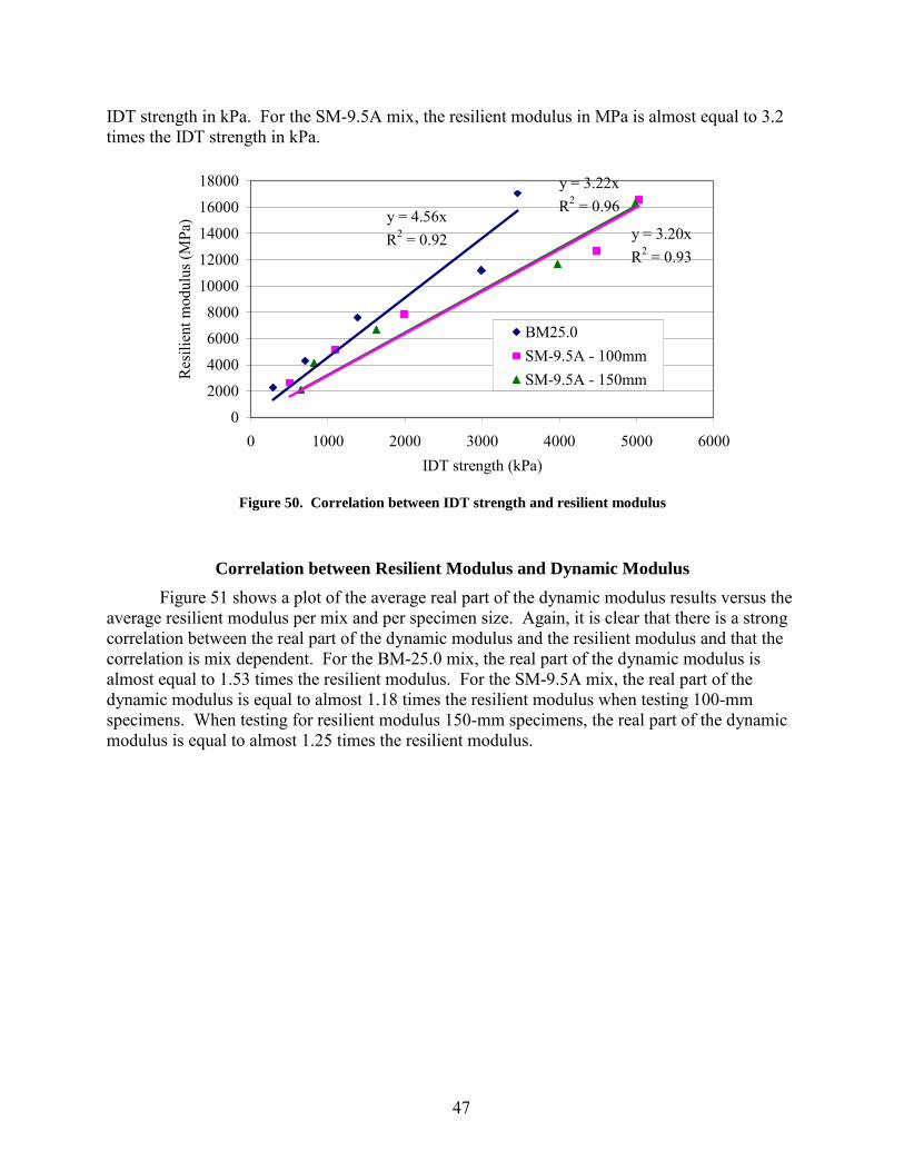
Correlation between Resilient Modulus and Dynamic Modulus Figure 51 shows a plot of the average real part of the dynamic modulus results versus the

average resilient modulus per mix and per specimen size. Again, it is clear that there is a strong correlation between the real part of the dynamic modulus and the resilient modulus and that the correlation is mix dependent. For the BM-25.0 mix, the real part of the dynamic modulus is almost equal to 1.53 times the resilient modulus. For the SM-9.5A mix, the real part of the dynamic modulus is equal to almost 1.18 times the resilient modulus when testing 100-mm specimens. When testing for resilient modulus 150-mm specimens, the real part of the dynamic modulus is equal to almost 1.25 times the resilient modulus.

48

y = 1.53R2 = 0.97 y = 1.18x

R2 = 0.97

y = 1.25xR2 = 0.95

0

5000

10000

15000

20000

25000

30000

0 5000 10000 15000 20000Resilient modulus (MPa)

E' (M

Pa)

BM25.0SM-9.5A - 100mmSM-9.5A - 150mm

Figure 51. Correlation between resilient modulus and elastic part of the dynamic modulus

FINDINGS

In this project, the IDT strength, resilient modulus, static creep in the IDT and uniaxial setups, flexural beam fatigue and dynamic modulus tests were conducted on two typical mixes used in the Commonwealth of Virginia: SM-9.5A and BM-25.0. The following are the main findings that can be drawn from the experiment:

Sample Preparation

�� The Vibratory Asphalt Compactor is not able to produce HMA beams with less than 7% voids for the SM-9.5A mix or less than 10% voids for the BM-25.0 mix.

IDT Strength

�� The IDT strength test is a simple test that produces data with relatively small variability.

�� As expected, for the ranges of temperatures studied, the IDT strength decreases with an increase in temperature.

�� The specimen size has no significant statistical effect on the measured IDT strength.

�� The two mixes studied have statistically different IDT strengths. The IDT strength of the SM-9.5A mix was found to be higher than that of the BM-25.0 mix at all temperatures.

Resilient Modulus

�� The measured deformations vary on both sides in the resilient modulus test. Averaging the results from both sides could generate reasonable results.

�� As expected, the resilient modulus decreases with an increase in temperature.

49

�� The size of the specimens was found statistically to affect the measured resilient modulus value. Resilient modulus values obtained in the 100-mm diameter specimens were higher than those obtained in the 150-mm diameter specimens at all testing temperatures.

�� No statistical differences were observed in the resilient modulus of the two mixes. This is probably due to the high variability in the resilient modulus testing within the same mix.

Static IDT Creep

�� Although extreme caution was always taken to align the specimen between the loading strips, for static IDT creep, differences in deformation measurements between both sides were high.

�� Creep compliance values obtained with the IDT setup were very small and appear to be unrealistic, especially at low loading times, when compared to typical HMA mixes. This is mainly due to the testing setup.

Beam Fatigue

�� The fatigue test using the flexural beam setup is a time-consuming test, but the results obtained with it are needed for mechanistic-empirical pavement design.

�� The fatigue life of the SM-9.5A mix is higher than that of the BM-25.0 mix in the tested strain level of the experiment (strains between 200 �m/m and 600 �m/m). It must be noted that the two mixes have different binder contents and air voids.

Dynamic Modulus

�� As expected, under a constant loading frequency, the magnitude of the dynamic modulus decreases with an increase in temperature; under a constant testing temperature, the magnitude of the dynamic modulus increases with an increase in the frequency.

�� At temperatures of -15°C, 5°C, and 20°C, the phase angle decreases as the frequency increases. At testing temperatures of 30°C and 40°C, the behavior of the phase angle as a function of frequency is more complex, due possibly to the binder networking and more aggregate contribution to the behavior.

�� At high frequencies (1 Hz to 25 Hz), the phase angle increases with an increase in temperature; at lower frequencies, the behavior of the phase angle with temperature is more complex.

�� A sigmoidal function can be used for modeling the dynamic modulus data with very good statistical fit.

�� The BM-25.0 mix has higher dynamic modulus than the SM-9.5A mix at all frequencies and at all tested temperatures.

50

Static Uniaxial Creep

�� The static creep test in the uniaxial setup is a simple test and produces a homogeneous state of stress within the specimen, which facilitates the interpretation of the results.

Correlations

�� There is a strong mix-dependent correlation between the resilient modulus and the IDT strength.

�� There is a strong, mix-dependent correlation between the real part of the dynamic modulus and the resilient modulus.

CONCLUSIONS

�� The IDT strength test is a good and simple test to characterize the tensile strength of HMA.

�� The compressive uniaxial dynamic modulus and the static creep tests are simple to conduct and analyze.

�� The dynamic modulus test provides a better characterization of HMA than the resilient modulus because it provides full characterization of the mix over temperature and loading frequencies.

RECOMMENDATIONS

The following tests are recommended for characterizing HMA for mechanistic-empirical pavement analysis and design:

�� IDT strength for characterizing the HMA susceptibility to thermal cracking.

�� Dynamic modulus for characterization of the constitutive behavior of the HMA over various temperature and loading frequencies encountered in the pavement.

�� Uniaxial creep for characterizing the permanent deformation characteristics of the HMA.

�� Flexural fatigue test for characterization of the fatigue properties of HMA.

The recommended tests would provide the properties needed to characterize the asphalt layers in the mechanistic-empirical pavement analysis and design procedures that are being implemented in the Commonwealth.

Since there were significant differences in the measured properties of the two mixes evaluated, more mixes commonly used in Virginia should be characterized using the recommended tests.

51

Other related potential research topics that should be considered include the following:

�� Evaluation of the effect of the binder type and the air-void content on the dynamic modulus.

�� Use of the results from the dynamic modulus test as a material performance indicator.

�� A compacting machine able to produce beams with air-void content as low as 4% is needed to characterize the fatigue life of the HMA mixes produced in the Commonwealth.

�� It is recommended to use the dynamic modulus data to verify the ability to obtain the creep compliance of HMA through transformation.

COSTS AND BENEFITS ASSESSMENT Materials characterization testing can be a valuable tool in pavement design. Mechanistic-empirical modeling can be used to predict the performance of a pavement. With this type of testing and modeling, the materials used in pavements will be of better quality and more durable to environmental and structural deterioration. A more durable pavement will aid in reducing the frequency and costs associated with maintenance.

ACKNOWLEDGMENTS

The authors acknowledge the contribution of the following individuals to the successful completion of the project:

�� Kevin McGhee and Troy Deeds from VTRC �� Billy Hobbs, Samer Katicha, and Myunggoo Jeong from VTTI �� Susanne Aref from the Statistics Department at Virginia Tech �� The project steering panel.

REFERENCES

American Association of State Highways and Transportation Officials. AASHTO T27-99, Sieve Analysis of Fine and Coarse Aggregates, Standard Specifications for Transportation Materials and Methods of Sampling and Testing, Part 2 - Tests, 20th Edition, Washington, DC, 2000, pp. 32�36.

American Association of State Highways and Transportation Officials. AASHTO T209-99, Theoretical Maximum Specific Gravity and Density of Bituminous Paving Mixtures, Standard Specifications for Transportation Materials and Methods of Sampling and Testing, Part 2 - Tests, 20th Edition, Washington, DC, 2000, pp. 642�650.

52

American Association of State Highways and Transportation Officials. AASHTO T166-00, Specific Gravity of Compacted Bituminous Mixtures Using Saturated Surface-Dry Specimens, Standard Specifications for Transportation Materials and Methods of Sampling and Testing, Part 2 - Tests, 20th Edition, Washington, DC, 2000, pp. 514�516.

American Society for Testing and Materials. ASTM D4123, Standard Test Method for Indirect Tension Test for Resilient Modulus of Bituminous Mixtures. Annual Book of ASTM Standards, Road and Paving Materials, Vol. 04, No. 03, Philadelphia, PA, 1998.

Huang. Pavement Analysis and Design. Prentice Hall, Upper Saddle River, NJ, 1993.

InstroTek Inc. CoreLok Operators Guide, 2003.

Kim, R.Y., Daniel, J.S., and Wen, H. Fatigue Evaluation of WesTrack Asphalt Mixtures Using Viscoelastic Continuum Damage Approach, Final Report. North Carolina Department of Transportation, Research Project No. HWY-0678, Raleigh, NC, 2002.

Loulizi, A., Al-Qadi, I.L., Lahouar, S., and Freeman, T.E. Measurement of Vertical Compressive Stress Pulse in Flexible Pavements and Its Representation for Dynamic Loading Tests. Paper No. 02-2376, Transportation Research Record, No. 1816, Transportation Research Board, Washington, DC, 2002, pp. 125�136.

Pellinen, T.K., and Witczak, M.W. Stress Dependent Master Curve Construction for Dynamic Modulus. Journal of the Association of Asphalt Paving Technologists, Vol. 71, 2002, pp. 281-309.

Roque, R., and Buttlar, W.G. Development of a Measurement and Analysis Method to Accurately Determine Asphalt Concrete Properties Using the Indirect Tensile Mode. Proceedings of the Association of Asphalt Paving Technologists, Vol. 61, 1992, pp. 304-332.

Witczak M.W., Kaloush, K., Pellinen, T., El-Basyouny, M., and Von Quitus, H. Simple Performance Test for Superpave Mix Design. NCHRP Report 465, Transportation Research Board, Washington, DC, 2002.