Standard Operating Procedures - Coral Reef Targeted Research

Standard Operating Procedures for repeated measures of process and state

variables of coral reef environments

Contributing authors: Robert van Woesik1, Jessica Gilner1, and Anthony J Hooten3.

Cover photos: Adán Guillermo Jordán-Garza

The Coral Reef Targeted Research & Capacity Building for Management (CRTR) Program is a leading international coral reef research initiative that provides a coordinated approach to credible, factual and scientifically-proven knowledge for improved coral reef management.

The CRTR Program is a partnership between the Global Environment Facility, the World Bank, The University of Queensland (Australia), the United States National Oceanic and Atmospheric Administration (NOAA) and approximately 50 research institutes and other third-parties around the world.

Coral Reef Targeted Research and Capacity Building for Management Program, c/- Centre for Marine Studies, Gerhmann Building, The University of Queensland, St Lucia, Qld 4072, AustraliaTel: +61 7 3346 9942 Fax: +61 7 3346 9987 Email: [email protected] Internet: www.gefcoral.org

1Florida Institute of Technology, 2AJH, Environmental Services.

Product code: CRTR 002/2009Editorial design and production: Currie Communications, Melbourne, Australia, September 2009. © Coral Reef Targeted Research and Capacity Building for Management Program, 2009 .

3

ContentsI. Introduction 5

II. The ecological context 7

III. Ecological field methods 7

A. Coral demography methods 9 Site selection and sampling structure 9 Data collection 10 Equipment 11

B. Coral demography photo analyses 13 Size measurements 13 Partial mortality 13 Benthic composition 13 Step by step directions for Sigma Scan Pro 14 Step by step directions for ImageJ 15

C. Coral recruitment methods 16 Data collection 16

D. Coral disease field methods 18 Equipment 18 Data collection 18

E. Fish recruit sampling methods 20 Equipment 20 Data collection 20 Estimating length exercises 21

F. Rate of herbivory methods 22 Data collection for fishes (optional) 22

IV. Data management 23

V. Contacts 25

Appendix A. Guidelines for image capture 26

Appendix B. Disease prevalence sheet 28

Appendix C. Coral reef fish censusing 29

Appendix D. Taxonomic Amalgamation Units 31

References 34

Standard operating procedures for repeated measures of process and state variables of coral reef environments

CRTR - Standard operating procedures

44

AcknowledgementsWe thank the following individuals who either participated, provided support, facilitation or helpful comments in the development of these Standard Operating Procedures:

Mehbrahtu Ateweberhan, Alasdair Edwards, Roger Green, Ed Gomez, Eric Jordán, Melanie King Nancy Knowlton, Margareth Kyewalyanga, Yossi Loya, Miguel Angel Maldonado, Brian McArdle Tim McClanahan, Christopher Muhando, Pete Mumby, Juan Carlos Ortiz, Roberto Iglesias-Prieto, Peter Sale, Paul Sanchez-Navarro, Gabrielle Sheehan, Robin Smith, Robert Steneck, Ali Ussi Saleh Yahya, Assaf Zvuloni.

We also thank the Herbert W. Hoover Foundation for providing funding to support the creation and management of a central database to be used by all CRTR Program locations.

I. Introduction The Coral Reef Targeted Research and Capacity Building for Management (CRTR) Program is an international initiative designed to improve the knowledge base to help sustain the world’s coral reefs for the future. The CRTR Program was conceived in 1998 to identify gaps in coral reef ecosystem knowledge and to establish more proactive (rather than reactive) approaches to environmental impacts. The main goal of the CRTR Program is to enhance current knowledge so coral-reef management is provided with improved options in managing risk.

The CRTR Program involves a network of over 70 international scientists representing more than 50 institutions worldwide, and is operating in four major world regions: Mesoamerica (Mexico); Southeast Asia (the Philippines), East Africa (Zanzibar) and Oceania (Australia) (Figure 1).

Within each region a Center of Excellence (CoE) has been engaged to enhance regional capacity for science-based management of coral reefs. The CoEs function as regional hubs, which create knowledge through research and training and disseminate information to an array of stakeholders, including local leaders and government, to facilitate informed decisions related to the use and protection of coral reefs. These regional hubs are in turn connected to the global network of scientists and institutions that serve as peer reviewers. These reviewers help synthesize the information at relevant scales, and strive to provide a source of credible and timely information about coral reefs to the public, and to local and national policy-makers.

Six thematic areas for targeted investigations were defined in consultation with managers and scientists around the world during the design of the CRTR Program. The themes serve as the technical foundation for the program and are defined as follows:

1. Coral bleaching and local ecological factors 2. Coral disease 3. Coral reef connectivity and large scale ecological processes 4. Coral reef restoration and remediation 5. Remote sensing 6. Modeling and decision support

MESOAMERICA

EAST AFRICA

PHILIPPINES

SOUTHERN GREAT BARRIER REEF

NorthAtlanticOcean

SouthPacificOcean

SouthPacificOcean

NorthPacificOcean

IndianOcean

5

Figure 1. Four CRTR regions and locations of the Centers of Excellence


6

A key task of the CRTR Program is to improve the integration of information across scientific experts, regions, time and space (Figure 2). One of the most practical ways to do so is to demonstrate where CRTR Working Groups can collect and share data to strengthen potential relationships across scales of investigation, and to minimize the redundant and unnecessary collection of some data. Equally important, is to identify a core set of variables to monitor in each region, which will provide opportunities for interaction between Working Group members, Centers of Excellence and regional researchers. Thus, the establishment of monitoring locations in and around each of the Centers of Excellence, where a set of key process and state variables can be measured, is an important dimension and legacy of the CRTR Program.

Working group collaboration and integration of findings at each study location

6

Figure 2. Potential for information integration between CRTR thematic areas and Working Groups. From molecular and physiological research, to organism, community and population dynamics, to seascape, regional and global levels, information can be shared across these scales to strengthen and apply new knowledge.

Legend BWG: Bleaching Working GroupCWG: Connectivity Working GroupDWG: Disease Working GroupRRWG: Restoration and Remediation Working GroupRSWG: Remote Sensing Working GroupMDSWG: Modelling and Decision Support Working Group

Modelling & Scenario Building for Decision Support

Remote Sensing to detect change. monitor trends, and enhance (improve) early warning

Connectivity and replenishment between coral reef ecosystems. Large-scale ecological processes.

Management of communities and ecosystems; restoration of degraded systems

Response to stresses; impacts on reproduction, recruitment, demography

Individual physiological responses (e.g. at the molecular/cellular level) such as bleaching, pollution and other forms of stress

BWGCWGDWGRRWG

BWGDWGRRWGRSWG

CWGRRWGRSWG

RSWG

MDSWG

BWGDWG

II. The ecological context Most reef studies and monitoring programs examine the state variables (i.e. coral cover, macroalgal cover, size-frequency distributions) of coral reefs, by assessing the coverage of major benthic organisms; few studies examine the key ecological processes that drive these state variables. Processes of major interest include recruitment rates, individual growth rates, partial mortality rates of clonal organisms, and survival. We are also interested in macro-processes such as predation, herbivory, and oceanography and their influence. Understanding these key processes, assessing their spatial variation and their relationship with state variables will lead to predictive models of population trajectories, relative population size distributions, and community change under different climate change scenarios. Yet, key processes that drive community composition differ in accordance with regional settings, and possibly among localities within regions. Furthermore, the key processes that drive community structure and population dynamics may also vary in their influence depending on the spatial scale of observation.

There is limited information on process variables, especially collected in a similar, systematic manner. Thus, there is a pressing need to establish and evaluate, through repeated measures, processes at localities that may lead to comparisons across spatial scales over time. Indeed, the significance of processes may change over time. These Standard Operating Procedures present a standard approach with which to collect state and process variables at the various habitats in the vicinity of each CoE and other satellite locations. These methods are intended to be rigorous enough to make useful comparisons among localities, yet flexible enough to allow for different analytical approaches, within the CRTR Program. Development of Standard Operating Procedures will provide a means for other regions and research groups to adopt these methods, minimizing the variation in data collection and facilitate our interpretation and understanding of coral-reef dynamics. Therefore, the overall objective of this document is to outline a field protocol, within the auspices of the CRTR Program’s network of scientists, which will allow comparisons of key state and process variables across three oceans.

III. Ecological field methodsThe sampling strategy outlined below captures both state and process variables at a spatial scale of tens of kilometers. Our sampling units are randomly selected 75 x 25 m stations, spaced approximately 250-500 m apart, representing a 103 m spatial scale. Stations are nested within

sites, which are spaced approximately 2 km apart, representing a 104 m spatial scale. In most cases we sample six to seven sites per location. Within each station we run at least five 50 m transects that are re-randomized at each sampling period, and used to estimate state variables (i.e. size frequency distributions, benthic composition, see Figure 3). Three randomly selected 16 m2 quadrats are placed in each station, and marked for relocation purposes, and used to assess processes (i.e. recruitment,

growth, partial mortality, mortality etc.) across time (repeated measures design, see Figure 3). Both quadrats and belt-transects are effectively sub-samples from which we will derive estimates of means for each station at each sampling event (because the station is the effective sampling unit).

7

Figure 3. Hierarchical sampling design with three quadrats and five transects in each station and two stations nested within each site. (Robert van Woesik & Jessica Gilner)

Site (n≤6)

Station a Station b

75m

25m50m to

500m


8

We focus sampling efforts to one depth zone (2-5 m) rather than stratifying the design by depth and reducing the spatial area to be sampled. We thoroughly appreciate that zonation is obvious on coral reefs (Darwin 1842), and hundreds of papers since Darwin’s famous prose have quantified the differences among coral reef habitats (i.e. reef flat, crest and slope).

We are also cognizant of the fact that state and process variables may differ with depth. However, the variation in zones can be considerable – not only locally, but certainly regionally – and across oceans. Therefore, at the initiation of the CRTR Program in 2005, we focused our sampling efforts to one depth (2-5 m) across four locations; but this sampling protocol can be easily adopted on reef flats and deeper zones.

The methods described below can be executed from the same platform (e.g. if access to the site is remote and requires a collaborative and integrated approach to data collection) or sampling, as described in each of the following sections, can be executed separately (e.g. on different dates). Investigators should keep in mind the potential disturbance to benthic and pelagic species and should coordinate sampling to minimize impacts.

9

A. Coral demography methods The coral demography field methods are designed to allow us to examine the driving forces behind changes in population structure and to investigate the composition of particular coral populations. Annual monitoring is conducted at approximately the same time of year.

Site selection and sampling structureThe sampling strategy captures state and process variables at each location, at a spatial scale of tens of kilometers. Sampling should aim to establish six to seven sites per location. Sites should be spaced approximately 2 km apart, with random stations nested within sites. Sites however should be systematically selected based on the targeted depth regime (2-5 m). Also, any sites that have ongoing studies for which there are historical data should be incorporated within the sampling. Sites must be selected as a representation of the habitat throughout the location. Once an adequate site is located, GPS coordinates are taken to aid relocation.

Two randomly selected stations should be established within each Site, whereby the station is the primary sampling unit. Each station will be approximately 1875 m2, where actual dimensions should be considered ‘plastic’ and dependent on the survey environment. Stations are considered small enough to be located using GPS, yet large enough to examine fluctuations in population dynamics and key processes. Where the reef slope is steep, a station would be elongated, whereas for a flat-reef terrain the station should be approximately 75 x 25 m. Therefore, dimensions are plastic while the total area (1875 m2) must remain rigid. Once the stations are established, the boundaries should be permanently marked (e.g. GPS, or permanent markers where permitted) and then sampled and re-sampled strictly within the defined dimensions. Since each station is randomly defined within a site, the distance between stations within sites will vary from 50 to 500 m. Again, the effective sampling units are stations, each of which are sampled annually. Notably, a mixture of random transects and permanent quadrats will be used to quantify the targeted process and state variables (Figure 3).

Once stations have been established and marked if fishes are to be censused at the time of sampling, the very first sampling should be for large or cryptic fishes (or other larger, mobile species). Refer to Section E for details.


10

Data collection

TransectsRandom-linear transects should be run using standard metric tapes to estimate state variables. At least five 1 m x 50 m belt-transects will be randomly placed in each Station. First, a line transect will be placed along the length of the Station (example: 75 m, if the station is 75 m long). Transects will be re-randomized during each sampling event. Excel® or another random generator should be used to randomly select transect location. Two sets of random numbers should be generated for each belt transect. Random numbers 1-25 and 50-75 m are generated which eliminates the middle area where a transect may not fit within the station dimensions. If the end result is too close to one edge, then the transect should be run in the opposite direction. The first being the starting point along the transect tape. The second number provides the distance one must travel at a 90° angle to begin the first transect (Figure 4). The belt-transect method quantifies the benthos as contiguous, and slightly overlapping (to create mosaics of 1 m2 images).

Figure 4. Randomization procedure used to place both transects and quadrats. (Jessica Gilner)

2

Station (1875m2)

1

2

Distance along 75m

Distance one swims at 90º angle from 75m transect

Starting point to run 50m transect

50m transect

75m1

11

Equipment1. Digital camera with an underwater housing, which will support an underwater wide-angle lens. 2. A ‘frame’ constructed to fit the chosen camera (Figure 5) • A frame is used to standardize the distance between the camera lens and substrate for all

photos to provide scale. The frame is best made of PVC and Lucite, but can be constructed with any available material (e.g. aluminum, acrylic):

- Camera must remain in the center of the quadrat, the images must capture the entire 1 m2 quadrat area, but should be at the minimal distance from the substrate to ensure high-resolution photos.

- Underwater housing must be equipped with a wide-angle lens otherwise the distance from the camera to the substrate is too great and resolution is lost.

• Frame construction: The most durable PVC has been found to be schedule 40 grey conduit. White PVC causes considerable haloing and blurs the pictures, thus reducing image quality.

- A minimum of 1” diameter PVC should be used. - The 1 m2 quadrat should be constructed using eight sections

Note: the exact length of each piece of PVC will depend on the couplers used, as couplers can add about 5 cm to total length.

- The corners of the quadrat will be joined using elbow joints and the vertical pieces that join to the camera plate should be joined with T-joints.

- The top of the frame should be also constructed with eight sections cut to a length that gives 40 cm total per side.

- The exact lengths will depend on the type of camera and wide-angle lens chosen. For ease of transport, the legs can be cut in half and joined with a coupler, but keep in mind durability will be lost.

- Centimeter markings (increments of 5 cm) should be made along the bottom of the frame for scale and calibration purposes.

•Camera bracing: - A piece of 12.7 millimeter Lucite should be used to brace the camera to the PVC frame. - The Lucite should be approximately 40 cm x 20 cm using some type of a glass-cutter or

a circular saw equipped with a glass cutting blade to avoid any cracking of the material - A semi circle should be cut in the center of one of the 40 cm sides to fit the camera.

Measurements should be taken to ensure that the lens fits directly in the center.

Figure 5. Example of camera-frame setup at Puerto Morelos, Mexico.


12

Digital images provide permanent records of the reef state, and allow retrospective and comparative sampling. Furthermore, photo-acquisition increases the spatial coverage of the reef for any given field session, although deriving data from the photos may be slower than actually recording the data in the field.

Permanent quadrats Permanent quadrats quantify the process variables (i.e., coral recruitment, growth and mortality rates, and herbivory). Within each station, three, 4 m x 4 m quadrats, should be established. The same randomization procedure used to demarcate belt-transect placement should be used for quadrat placement. Quadrat perimeters should be temporally demarcated using PVC pipe or rope (Figure 6a and 6b). In locations where permitted, stakes should be placed at each corner of each quadrat, and one in the center. Quadrats should be photographed twice. First, using the camera and frame, and second, without the frame. Each image in the second round of photos should overlap by 70% with adjacent images. This technique is useful for mosaicing. Camera calibration (see Appendix A ) will facilitate mosaicing.

Figure 6a. PVC pipe was assembled underwater and used to temporarily demarcate the boundaries of the 4 m x 4 m quadrat. Make sure that all PVC is removed after field surveys. Photo: Jessica Gilner

Figure 6b. Here rope was used to temporarily demarcate the boundaries. Make sure that all rope is removed after the boundaries have been successfully marked. Photo: Rob van Woesik

13

B. Coral demography photo analysesDigital photos should be analyzed using Sigma Scan Pro or ImageJ (both free software packages). Also, VidAna (developed under the auspices of the CRTR Program) can be used for determining percentage cover and area/perimeter ratios of quadrats and is freely available from http://www.ex.ac.uk/msel. A number of colonies will fall outside of the quadrat, yet within the photo, or a colony will take up more than just the 1 x 1 m quadrat, or colonies will fall along the edges with part of the colony within and part of the colony outside the quadrat. The best method to address these issues is to only identify and record coral colonies if their centers lie within the quadrat. There are considerable biases in popular and traditional sampling methods (e.g., quadrat, belt and line-transect) where size-frequency distributions suffer from boundary effects, yet the ‘center-rules’ method minimizes these biases and provides the most accurate size-frequency distributions. However, in regions where the ‘center rules’ cannot be used because of very large colony sizes, all colonies should be measured and the proper correction according to Zvuloni et al. (2008) should be applied to the dataset. Zvuloni et al (2008) provide an online supplementary Excel® spreadsheet that allows researchers to correct for biases. If these corrections are not applied then size-frequency distributions will not be accurate representations and the results will be unreliable. For our purposes, a coral colony is defined as a mass of continuous living tissue, rather than a structural mass. Corals should be identified to the highest taxonomic resolution (species where possible).

Size measurementsThe maximum diameter of each section of continuous-live tissue, and the maximum width 90 degrees to the maximum diameter, will be a useful estimate of coral-colony size. The area of the colony should be estimated with the assumption that coral colonies generally take on an elliptical geometry (Loya et al. 2001). In the event of partial mortality within a coral colony, all tissue isolates, (i.e. areas that are not connected by live tissue) are to be measured using the same procedure and recorded as separate colonies. This definition is useful because it agrees with physiological examinations which have shown that tissue disconnection changes life-history functions. However, the tissue isolates will be noted using a colony ID to track ramets (fragments of a genotype) and genets (of the same apparent genotype). Within the database, all tissue isolates will be given the same genet ID code. (refer to section IV for details).

Partial mortalityAreas of enclosed partial mortality are straightforward to record, whereas areas of partial mortality that appear at the edge of a coral colony are more difficult to record. In the former case, the area enclosed by continuous live tissue should be measured by tracing around the perimeter of the dead area. In the latter case, and to ensure repeatability, measurements will be limited to a working definition of peripheral mortality: if 50% or more of the perimeter of partial mortality is in contact with continuous live tissue, then the area can be measured. If less than 50% is in contact with live tissue, then the area cannot be accurately measured.

Colony ID is used to link the partial mortality data sheet with the colony size datasheet. If a colony is intact, with no partial mortality, then the colony ID is labeled as a single number corresponding to that single measurement. If however, there is partial mortality that separates the colony into different live tissue isolates, then each isolate will be given the same colony ID, to distinguish small coral colonies from ones that are remnants of once larger colonies. Size-frequency distributions will then be constructed for each population, but ramet and genet contributions can calculated, at least for the sampling period. Such estimates are useful because they identify rates at which ramets are being produced.

Benthic compositionTo measure benthic composition, ten crosses can be randomly placed on a computer screen; or use the freely available CPCe, Coral Point Count with Excel Extension® program (available at http://www.nova.edu/ocean/cpce/). These random points will overlay each 1 m2 quadrat. The organism or substrate type found directly under the cross, where the lines intersect (or point) will be recorded. Options include but are not limited to: CaCO3 (with turf algae), rubble (<70 cm), sponge, zooanthid, gorgonian, coral, macroalgae, urchin, sand etc.


14

Step by step directions for Sigma Scan Pro1. Open Sigma Scan Pro program. (Should have a tool bar at the top and an untitled data sheet

at the bottom).

2. Open the desired image by clicking on the folder button on the toolbar or File, Open, Image.

3. Then go to Measure Trace measurement options. (This will open the Trace Measurement Options dialogue box)

•Now depending on what you are interested in measuring you need to select that parameter from the available measurements column and then click “add” at the bottom to move that selection into the active measurement column.

•In the active measurements box there is a column (Col) area that indicates where the desired measurement will be recorded in the Sigma Scan Pro data sheet. This can be changed along with colors etc.

4. Once everything is set as desired click “OK”.

•For accurate measurements the image must be calibrated to a known scale in the photo.

5. Go to Measure Calibrate Distance and Area. (This opens the Calibrate Distance and Area dialogue box)

•Then select the 2 Point – Rescaling option. •Leave old distance as is and then change new distance to the known distance that is in the

photos (ex: 100 cm for the edge of a 1 x 1 m quadrat). •In the X,Y and Distance Units box at the bottom type in the units of the known distance. •Click on the Image button in the Calibrate dialogue box. •This allows you to select two points on your image. (The ends of your known distance).

Note: The point is at the arrowhead.

6. Once the image is calibrated click “OK” on the dialogue box.

Measurement of maximum diameter and width7. Scan the image for a coral colony by zooming in two to three times.

8. Then once a colony is located, identify the species and record on the data sheet.

9. To measure the maximum diameter, determine by eye the longest area of live tissue.

10. Then use your mouse and click on one side of the colony, then release and click on the opposite end of the colony, then right click. The measurement will be automatically placed in the Sigma Scan Pro spread sheet. Transfer this information to the data sheet.

11. The maximum width must be measured 90 degrees from the maximum diameter measurement. Use the same procedure to measure and record on the data sheet.

Measurement of partial mortality12. The colony ID column is used to link the partial-mortality data sheet with the colony-size

datasheet. If a colony is intact with no partial mortality then the colony ID is labeled as a single number corresponding to the single measurement. If there is partial mortality that separates colonies, each live-tissue isolate is given the same colony ID, but a unique code on the partial-mortality datasheet.

13. To measure the area using Sigma Scan Pro you will use the same trace tool used to measure maximum diameter and width.

14. Connect lines by left clicking at each perimeter’s ‘corner’ until the entire perimeter is traced and then close the area, then right click to fill the area. The area measurement will be placed in the area column on the Sigma Scan Pro spreadsheet.

15

Measurement of benthic composition15. Ten crosses (or points) will be randomly placed on a transparency or computer screen. These

points (if on a transparency) will be placed over the computer screen showing a 1 x 1 m quadrat.

16. The organism or substrate type that is found directly where the cross lines intersect will be recorded.

Step by step directions for ImageJ1. Open the ImageJ program, which can be downloaded as freeware from http://rsb.info.nih.gov/ij/

2. Select “File” then “Open” and navigate through the files to the folder containing the desired photos and select the individual photo.

3. Once the photo is loaded, it must be calibrated for further measurements. Here you must ensure that the photos are undistorted, which results from the wide-angle lens. PTlens® is a useful program to remove lens-related distortion for any given camera and lens: http://epaperpress.com/ptlens/

4. To calibrate the image, select the line tool from the toolbar menu. Then measure an area on the image of known length. Select “Analyze”, then “Set Scale”. The distance in pixels of the area you just measured will be given, then type in the known distance of that measurement. Calibration for future images loaded in the same Image J session.

Measurement of maximum diameter5. To measure maximum diameter and width use the straight-line tool. Click on one end of the coral

colony, and drag to the other end, and then let up. To get the measurement go to “Analyze” then “Measure” and it should pop up in a separate window. Once the measurement is visible ensure that it makes sense. For example, does a colony that takes up half of the quadrat measure at 50 cm?

Measurement of partial mortality6. To measure partial mortality, use the freehand selection tool. Click and trace around the desired area.

To obtain the measurement again select “Analyze”, then “Measure” and record on the data sheet.

Measurement of benthic composition7. Ten points (crosses) will be randomly placed on a transparency. These points will be placed

over the computer screen showing a 1 m2 quadrat. The organism or substrate type that is found directly where the cross lines intersect will be recorded. Options include but are not limited to: CaCO3 (with turf algae), rubble (<70 cm), sponge, zooanthid, gorgonian, coral, macroalgae, urchin, sand and other invertebrates.


16

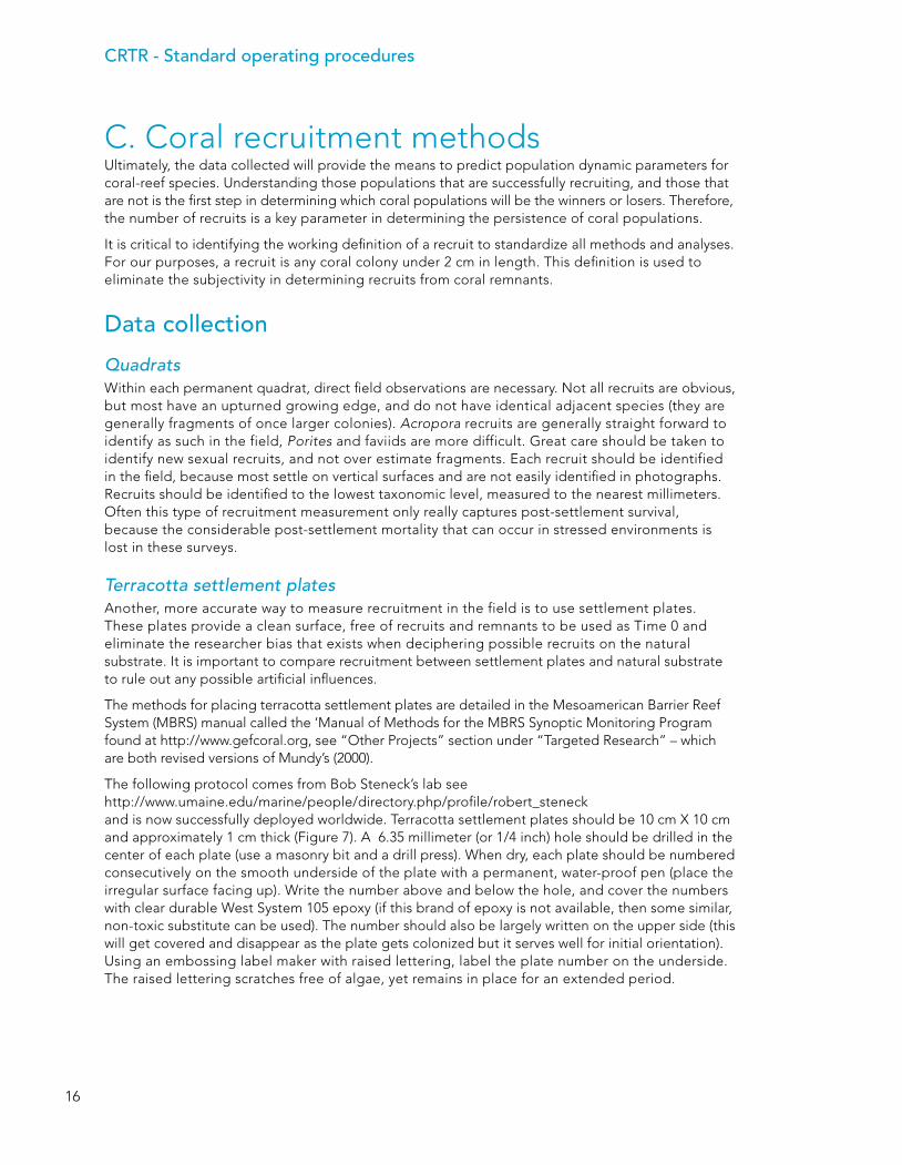
C. Coral recruitment methodsUltimately, the data collected will provide the means to predict population dynamic parameters for coral-reef species. Understanding those populations that are successfully recruiting, and those that are not is the first step in determining which coral populations will be the winners or losers. Therefore, the number of recruits is a key parameter in determining the persistence of coral populations.

It is critical to identifying the working definition of a recruit to standardize all methods and analyses. For our purposes, a recruit is any coral colony under 2 cm in length. This definition is used to eliminate the subjectivity in determining recruits from coral remnants.

Data collection

QuadratsWithin each permanent quadrat, direct field observations are necessary. Not all recruits are obvious, but most have an upturned growing edge, and do not have identical adjacent species (they are generally fragments of once larger colonies). Acropora recruits are generally straight forward to identify as such in the field, Porites and faviids are more difficult. Great care should be taken to identify new sexual recruits, and not over estimate fragments. Each recruit should be identified in the field, because most settle on vertical surfaces and are not easily identified in photographs. Recruits should be identified to the lowest taxonomic level, measured to the nearest millimeters. Often this type of recruitment measurement only really captures post-settlement survival, because the considerable post-settlement mortality that can occur in stressed environments is lost in these surveys.

Terracotta settlement platesAnother, more accurate way to measure recruitment in the field is to use settlement plates. These plates provide a clean surface, free of recruits and remnants to be used as Time 0 and eliminate the researcher bias that exists when deciphering possible recruits on the natural substrate. It is important to compare recruitment between settlement plates and natural substrate to rule out any possible artificial influences.

The methods for placing terracotta settlement plates are detailed in the Mesoamerican Barrier Reef System (MBRS) manual called the ‘Manual of Methods for the MBRS Synoptic Monitoring Program found at http://www.gefcoral.org, see “Other Projects” section under “Targeted Research” – which are both revised versions of Mundy’s (2000).

The following protocol comes from Bob Steneck’s lab see http://www.umaine.edu/marine/people/directory.php/profile/robert_steneck and is now successfully deployed worldwide. Terracotta settlement plates should be 10 cm X 10 cm and approximately 1 cm thick (Figure 7). A 6.35 millimeter (or 1/4 inch) hole should be drilled in the center of each plate (use a masonry bit and a drill press). When dry, each plate should be numbered consecutively on the smooth underside of the plate with a permanent, water-proof pen (place the irregular surface facing up). Write the number above and below the hole, and cover the numbers with clear durable West System 105 epoxy (if this brand of epoxy is not available, then some similar, non-toxic substitute can be used). The number should also be largely written on the upper side (this will get covered and disappear as the plate gets colonized but it serves well for initial orientation). Using an embossing label maker with raised lettering, label the plate number on the underside. The raised lettering scratches free of algae, yet remains in place for an extended period.

17

In regions where permitted, settlement plates should be fixed in the field by drilling a hole into the dead coral substrate and inserting a plastic wall anchor into which a stainless steel bolt can be screwed (Figure 7). However, in regions where drilling into the reef is not permitted plates must be fixed to a removable stand and placed in both vertical and horizontal positions as it has been documented that many corals recruit onto vertical surfaces. Recruitment and post-settlement mortality will be measured both within the permanent quadrats and on the terra cotta settlement plates. The settlement plates should be placed near each corner of each permanent quadrat for ease of relocation and to ensure precise comparisons with the natural substrate within the quadrats. Plate placement should also be mapped before leaving the station.

Figure 7. Recruitment plate six months after deployment in the field.


18

D. Coral disease field methodsSince the early 1970’s when white band disease took a toll on Caribbean acroporids there has been an exponential increase in the number of reported diseases and the number of locations with disease observations. Therefore, the CRTR Program designated a Coral Disease Working Group to fill in critical information gaps regarding coral reef diseases. Research priorities include assessing the global prevalence of coral disease, investigating the environmental drivers of disease and understanding the coral’s ability to resist disease. For a more complete discussion and detailed information regarding coral diseases, refer to the Coral Disease Handbook: Guidelines for Assessment Monitoring and Management (Raymundo et al. 2007).

EquipmentEach researcher should be equipped with the following equipment for disease data collection:

1. Data sheets (Appendix B) printed on underwater paper 2. Transect tape measures or 10 m rope with meter demarcations 3. Pencil 4. Flexible one meter tape with centimeter markings to measure individual colonies 5. Two, 1 m sections of PVC used to create one meter quadrats along the 10 m transect tape 6. Coral disease ID cards 7. Coral species ID cards 8. Differential GPS 9. Magnifying lens 10. Plastic caliper and ruler 11. Digital camera

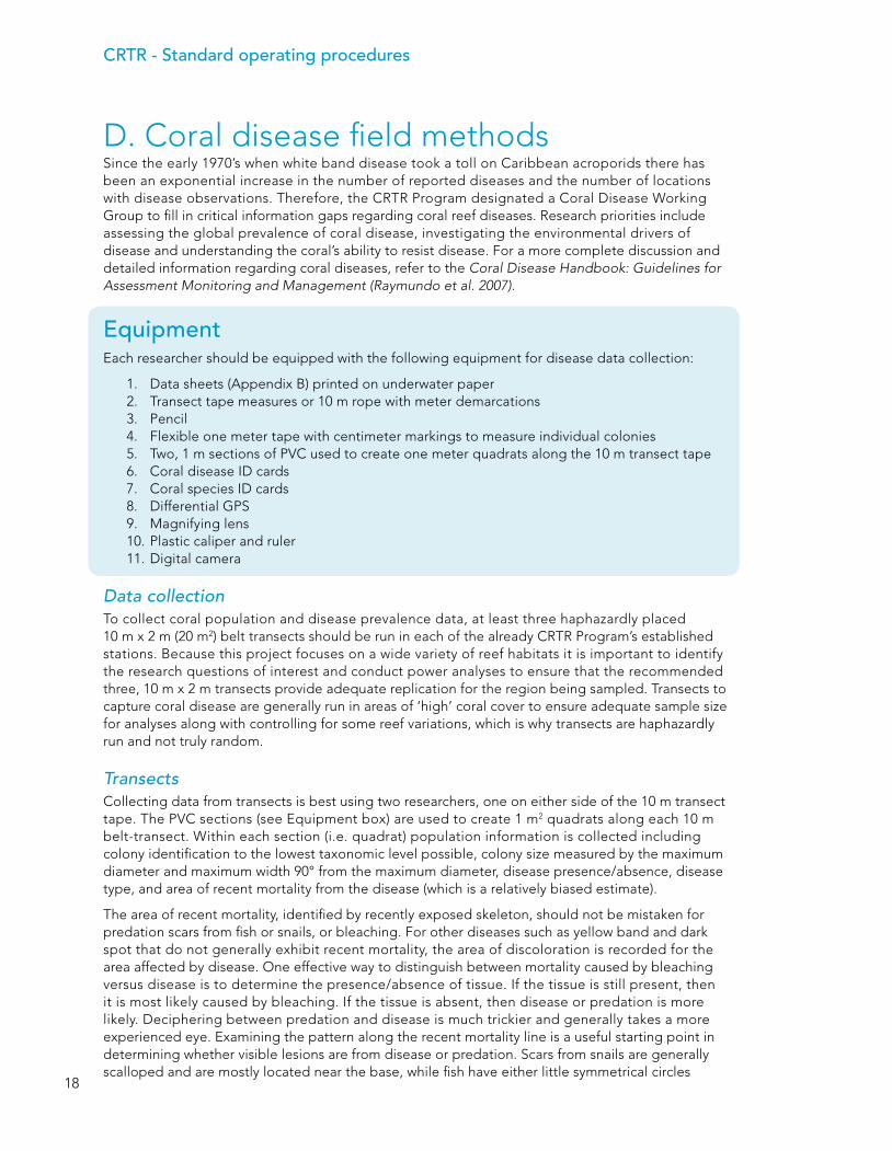
Data collectionTo collect coral population and disease prevalence data, at least three haphazardly placed 10 m x 2 m (20 m2) belt transects should be run in each of the already CRTR Program’s established stations. Because this project focuses on a wide variety of reef habitats it is important to identify the research questions of interest and conduct power analyses to ensure that the recommended three, 10 m x 2 m transects provide adequate replication for the region being sampled. Transects to capture coral disease are generally run in areas of ‘high’ coral cover to ensure adequate sample size for analyses along with controlling for some reef variations, which is why transects are haphazardly run and not truly random.

TransectsCollecting data from transects is best using two researchers, one on either side of the 10 m transect tape. The PVC sections (see Equipment box) are used to create 1 m2 quadrats along each 10 m belt-transect. Within each section (i.e. quadrat) population information is collected including colony identification to the lowest taxonomic level possible, colony size measured by the maximum diameter and maximum width 90° from the maximum diameter, disease presence/absence, disease type, and area of recent mortality from the disease (which is a relatively biased estimate).

The area of recent mortality, identified by recently exposed skeleton, should not be mistaken for predation scars from fish or snails, or bleaching. For other diseases such as yellow band and dark spot that do not generally exhibit recent mortality, the area of discoloration is recorded for the area affected by disease. One effective way to distinguish between mortality caused by bleaching versus disease is to determine the presence/absence of tissue. If the tissue is still present, then it is most likely caused by bleaching. If the tissue is absent, then disease or predation is more likely. Deciphering between predation and disease is much trickier and generally takes a more experienced eye. Examining the pattern along the recent mortality line is a useful starting point in determining whether visible lesions are from disease or predation. Scars from snails are generally scalloped and are mostly located near the base, while fish have either little symmetrical circles

19

and/or scrapes. For a more complete description of diseases and possible factors that could be mistaken as disease lesions, refer to the Coral Disease Handbook: Guidelines for Assessment, Monitoring and Management (Raymundo et al. 2007).

Colony taggingThe belt-transect method provides more of a rapid assessment of state variables while monitoring individual colonies provides detailed information for a limited number of colonies. Coupling rapid assessments and colony monitoring is useful when asking questions regarding the reef status along with disease progression among individual colonies. Individual colonies can be monitored in the permanent quadrats. Other colonies outside of the quadrat can also be tagged and monitored to increase sample size or target a specific species that is not adequately represented in the quadrats. To monitor the rate of progression, the method for tagging varies based on the growth morphology. If the colony is of the branching morphology, then a cable tie is placed right below the progressing band (Figure 8). If the colony is of massive or encrusting formation, a nail driven into the dead skeleton (Figure 9) just below the progressing band could demarcate disease location and would be useful to estimate disease progression rate. A GPS point should be taken along with a map drawn complete with photographs should also be taken to aid relocation of the colonies. Benthic composition information (i.e. coral id, coral rubble, dead standing coral, pavement with turf algae, rock, macroalgae, soft corals, sand, silt and sponges) is also usually taken using replicated line-intercept transects.

Figure 8. A branch of Acropora with white syndrome. The green cable tie marked the original position of the band when it was first observed and was used to measure disease progression. Photo: L. Raymundo

Figure 9. A masonry nail (arrow) hammered into dead skeleton can provide a useful reference point and scale for monitoring disease progression in an active lesion. Here a massive Porites colony exhibits signs of white syndrome. Photo: L. Raymundo.


20

E. Fish sampling methodsMeasuring both adult and recruitment of coral reef fish within each station provides useful information about the population dynamics and demography for the area investigated, if assessed repeatedly over successive years. The methods described below are not as advanced or detailed as those for coral recruitment. Sampling fishes is obviously complicated by the fact that they frequently move; however, these methods have provided useful data to compare population dynamics over time.

Prior to sampling fish adults or recruits, samplers should consider counting the larger and more cryptic fish that may occur within a station. Upon arriving at a station for sampling, fish observers should first confirm the station dimensions and should enter the water with intent to scan the entire boundaries and interior of the 25 m x 75 m station and record the presence of any large individuals, such as exploited groupers, Bolbometapon or Scarus guacamaia (as examples). The individuals of interest will obliviously vary by region, but these should be investigated first given their tendency to flee after divers are in the water for extended periods. Then the sampling of adults and recruits should follow as per the following procedures.

Recruitment of coral reef fish should be estimated at each station only once per year; however, this should occur at the same time every year and should take place during the “end of summer” for each region (for example, in Australia, this would be in March; in the Caribbean, this would be during September). Sampling should also be within the first seven days following the new moon phase. Although many fish species vary in their most abundant recruitment periods, this consistent timing of sampling provides the best overall indication of the majority of new fish that will have successfully established within a coral reef system. Also, sampling should occur at low tide to further reduce the variability in observations. The best times for sampling is between 10 am and 3 pm whenever possible. If gaps in data occur, they should be noted and briefly described.

EquipmentEach diver will need to carry:

1. Two underwater data templates for fish (Appendix C) per station 2. Plastic underwater slates 3. Two 30 m fiberglass surveying tapes or 30 m rope attached to a reel with a clip 4. Two 3 lb (or 1 kg each) weights to weight the end of the tape 5. Underwater cards to aid species identification

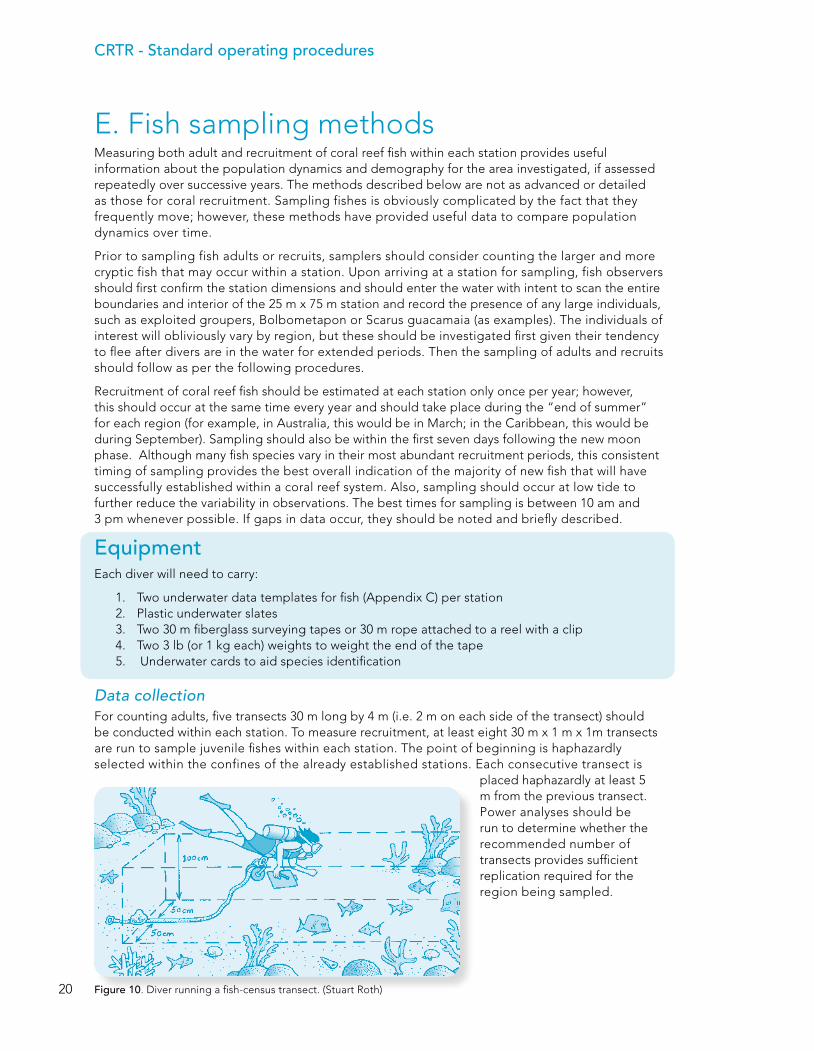
Data collection For counting adults, five transects 30 m long by 4 m (i.e. 2 m on each side of the transect) should be conducted within each station. To measure recruitment, at least eight 30 m x 1 m x 1m transects are run to sample juvenile fishes within each station. The point of beginning is haphazardly selected within the confines of the already established stations. Each consecutive transect is

placed haphazardly at least 5 m from the previous transect. Power analyses should be run to determine whether the recommended number of transects provides sufficient replication required for the region being sampled.

Figure 10. Diver running a fish-census transect. (Stuart Roth)

21

For each transect within the station:

1. The recorder’s name, date, time transect is started, site and station name, GPS location, and transect number is recorded on the datasheet provided.

2. To run these transects, the weighted end of the line must first be placed on the bottom (Figure 10). A special weighted transect is used and laid as the researcher is swimming so that it is behind the research, which minimizes any disturbance to the fishes.

3. Then with the transect clipped to your weight belt, or get a diver to follow you with the transect line, swim in a straight line by periodically focusing on a fixed object while releasing the tape from the reel as you count all the coral reef fish recruits found within a 1 m wide visually estimated belt transect.

It is best to swim along depth contours and along spurs to minimize depth changes. Each researcher must carry a data sheet on underwater paper, pencil and weighted transect tape, (Figure 10). The transect belt should be sampled by giving equal attention to each successive 2 m segment. This requires swimming at a more or less constant rate, while looking consistently 2 m ahead of your current position. However, high densities of counted fish species will slow this rate. Only individuals that are actually within the 1 m wide strip should be included in the census, even when counting a school.

Fish observers should be trained to estimate fish lengths by using consistency-training methods found below. Because fish recruits are cryptic they are harder to spot, therefore researchers should try to swim each transect 1 to 1.5 m over the substrate. Care should be taken to ensure that your fins do not accidentally come into contact with the reef or substrate.

For the Caribbean, only the species listed in Appendix C, should be counted to satisfy the requirements for the CRTR Program. Checklists for Indo-Pacific species can be downloaded at www.gefcoral.org, see “Other Projects” section under “Targeted Research”. Some researchers may wish to census other species of fish not listed in the table for specific research questions. This is of course encouraged provided that these other species are counted on a separate pass over the transect. Otherwise, the census method will be substantially changed, and the data will not be directly comparable with other assessments. (These should be performed prior to and separate from sampling at the stations.)

Estimating length exercisesSince we do not attempt to catalogue every fish by their actual size all we need to do is be comfortable with estimating the maximum length and then recording every fish smaller that is found within the transect. For this we suggest two field exercises that will train your underwater size estimation skills. (These should be performed prior to and separate from sampling at the stations.)

Exercise 1: In this exercise, observers practice fish counting along a belt transect and estimating fish size. Each observer should have a T-bar (with 5 cm increments), a 30-m transect tape, and a datasheet. A practice transect line is laid on the substratum and fish models (made from drinking straws of various lengths that are attached to a weighed line) are haphazardly placed along the transect. One observer starts at the beginning of the transect line and uses a T-bar to estimate the width of the 1 m belt transect and the length of fish. Observers should mark on their data sheet the estimated size for each model observed in the sample area. Each observer should run the survey. After completing the exercise, compare the answers of all the observers with the correct fish lengths. Repeat exercises until observers are consistent between each other and their answers are close to the correct answers. We suggest cutting the straws at 0.5 cm increments starting at 1 cm and going to 5 or 6 cm. this way you will be able to estimate sizes longer than the maximum total length for each species. Data analysis should be by means of a linear regression between the estimated length and the real length of the model. The r² value will give an estimate of precision, whereas the slope will give an estimate of accuracy.


22

Exercise 2: Each observer will carry an underwater slate and a plastic measuring rule. The objective of this exercise is to estimate the size of an inanimate object and then compare this estimate to the actual length of the object. While drifting through the area identify small pieces of rubble or other small structures and try to estimate their length, then pick up the object and measure its length. Try to collect fusiform objects since these will mimic a fish’s shape. This exercise differs from Exercise 1 in that while the straws come in 5 mm increments, fish rarely do, therefore you will be able to better estimate actual lengths rather than size classes. Analyze the data in the same way as for Exercise 1 to obtain your accuracy and precision values.

F. Rate of herbivory methods The top priority for measuring rates of herbivory is to get good fish and urchin censuses by species, body size (actual standard length rather than size categories), and life phase. For fishes, it is appropriate to use 30 x 4 m transects (n=10) to predict total grazing and to quantify the grazing rate of species at size X. An optional census technique involves independent measures of grazing, whereby one deploys 1 m imaginary quadrats and to then quantify the number of bites x fish species x size x phase (i.e. terminal, intermediate phase, and juvenile phase) within 5 minute observations (Steneck, 1985). Do as many quadrats as possible within a dive. The objective is to gauge the effect of herbivorous fishes on algal composition by quantifying their level of herbivory. These data are highly variable, particularly when fish abundance is low: fish census using the 30 m transects is probably more useful. For urchins, use random 1 m2 quadrats within each station. Undertake a power analysis on pilot data to make sure there is sufficient replication; 25 replicate quadrats per station is sufficient in most regions. In addition to, or alternatively, you may census the entire 16 m2 area of permanently marked station quadrats established and discussed under section III.

Data collection for fishes (optional)1. Use a 1 meter stick in conjunction with natural features on the reef (e.g. a small coral or

gorgonian) to haphazardly delineate an area that is approximately 1 m square (do not mark or place a meter quadrat or other feature over the designated area, as some fish are particularly prone to biting novel objects placed within their feeding territories).

2. Back off as far as you can while still being able to see the meter square area. Watch for five minutes. Time of day, and number of bites from all species of fish from the three guilds listed above (identify the fish to species, if possible). Repeat for a total of five squares (and 25 minutes of observation). Note: you must be able to distinguish:

a. Juvenile scarids from other fishes with similar stripes, such as acanthurids and labrids (i.e. wrasses – which appear as if they are biting algae as they search for amphipods and other small crustaceans), and

b. Yellowtail damselfish (which are browsers) from other species of damselfish (that cultivate algal gardens). Be sure to remember to record the time of day, since fish activity varies temporally.

c. Different functional forms of parrotfishes including escavators (the genus Sparisoma in Caribbean, and genera Bolbometapon, Chlorurus, Microrhinus, and Cetoscarus in the Indo-Pacific) and scrapers (genera Scarus and Hipposcarus).

d. All juvenile Nasos and herbivorous adult Naso species such as lituratus and unicornis (Indo-Pacific), and

e. Rabbitfishes (Indo-Pacific) and surgeonfishes from non-herbivorous fishes of similar size like angelfishes.

23

IV. Data managementThe amount of data the CRTR Program has collected and will continue to collect is immense. Successful completion of objectives and global comparisons relies on quality control and data management starting early and continuing throughout the Program. This will ensure that all regions are collecting data required for the targeted comparisons. Microsoft Access® has been used to create a relational database where data from all regions will be entered and kept at the Florida Institute of Technology as a central repository (however, database copies will reside with each CoE). Using the same database throughout all CoEs will provide a means of quality control to ensure all required data is collected and entered, and will ease global comparisons without wasting time deciphering individual’s Excel worksheets.

Communication between CoEs and data sharingData will be requested from all CoEs by the Data Coordinator every year and should be provided in a timely fashion already entered into their copy of the Access database. Progress updates should also be provided to the data coordinator and program lead on a regular basis (preferably, monthly and more frequently if determined by either party). The Access database will be shared within the group to answer targeted questions posed either by the group or for individual dissertations or projects. Once results are published, then sharing with other groups and/or programs will be assessed on a case-by-case basis.

Database set-upMicrosoft Access allows you to create multiple tables that can then be linked together by shared data columns containing specific attributes related to sites and stations. This allows the researcher to query specific information based on these shared attributes, thus creating new spreadsheets ready for analysis within minutes. This database makes it possible to summarize large amounts of data into simplified reports within seconds. The key to successful queries lies in the proper linkage of data-tables through clear definition and shared attributes (e.g. similar columns in each separate table to be linked). The database description below indicates the key fields of data needed for sites and stations. They are accompanied by examples of how datatables are presented within Microsoft Access.

SiteID Station Name Code Latitude Longitude Average

DepthGeographical Region Code

Map Datum

1 Bocana PM1 0 0 2 M

2 La Ceiba PM2 0 0 1 M

3 Jardines PM3 0 0 2 M

4 Akumal Site 1 AK1 0 0 2 M

5 Akumal Site 2 AK2 0 0 2 M

Example of Microsoft Access table view for sites (data from the Caribbean region shown).


24

StationID Station Name Station Code Site Code Latitude Longitude Geographical

Region Code

1 Bocana Outer PM1a PM1 0 0 M

2 Bocana Lagoon PM1b PM1 0 0 M

3 La Ceiba PM2a PM2 0 0 M

4 Ojo PM2b PM2 0 0 M

5 Jardines North PM3a PM3 0 0 M

6 Jardines South PM3b PM3 0 0 M

7 Akumal Site 1 Station 1 AK1a AK1 0 0 M

8 Akumal Site 1 Station 2 AK1b AK1 0 0 M

9 Akumal Site 2 Station 1 AK2a AK2 0 0 M

10 Akumal Site 2 Station 2 AK2b AK2 0 0 M

Example of Microsoft Access table view of stations that are part of sites (Bocana station data shown).

Database definitionThe following are a listing of the data fields required for the CRTR relational database:

Station - ID - Station name - Station code - Site code - Latitude - Longitude - Geographical region

Photo code - ID - Photo number - Photo name - Photo code

Depth - ID - Depth range - Depth zone code

Species - ID - Abbreviation - Species - Genus code - Family code

Time period - ID - Time period - Time code

Geographical region - ID - Geographical region - Code

Genus codes - Code (ID) - Genus - Family

TAU - ID - TAU name - TAU family members - TAU genus members - TAU code - Species - TAU order - Morphology - TAU example

(links to photos)

Site - ID - Site name - Code - Latitude - Longitude - Average depth - Geographical region - Map datum

Permanent quadrat description - ID - Permanent quadrat ID - Time - Geographical region - Site code - Station code - Latitude - Longitude - Permanent quadrat code - Map datum - Quadrat name - Photo code - Management status - ID - Management status - Site code

Family - ID - Family

25contacts

V. ContactsProgram coordinationRob van Woesik , Program Lead & Coordinator Florida Institute of Technology 150 W. University Blvd., Melbourne, FL 32901 [email protected]

Jessica Gilner , Data Coordination and Communication Florida Institute of Technology 13204 Agave St., Panama City Beach, FL 32407 [email protected]

Team membersMesoamerica

Jessica Gilner, Florida Institute of Technology, USA, [email protected]

East Africa

Dr. Christopher Muhando, University of Dar es Salaam, Tanzania, [email protected]

Dr. Yossi Loya, Tel Aviv University, Israel, [email protected]

Assaf Zvuloni, Tel Aviv University, Israel, [email protected]

Omri Bronstein, T el Aviv University, Israel, [email protected]

Philippines

Dr. Wilfredo Licuanan, De La Salle University, Phillippines, [email protected], licuananw@dlsu edu.ph

Mark Vergara, University of the Philippines, [email protected]

Oceania

Prof. Ove Hoegh-Guldberg, University of Queensland, Australia, [email protected]

Juan Carlos Ortiz, University of Queensland, Australia, [email protected]


26

Appendix AGuidelines for capturing images for camera calibration and mosaics

Camera calibrationCamera calibration allows for correcting geometric distortions induced by the camera lens and housing. This calibration is based on processing a set of images of a calibration grid taken underwater. The grid is a flat-checkered pattern that can be found at the following web-address (http://www.vision.caltech.edu/bouguetj/calib_doc/htmls/pattern.pdf). The calibration procedure is done using Matlab® using the camera calibration toolbox, which is freely available on the web (http://www.vision.caltech.edu/bouguetj/calib_doc/).

Camera calibration checklist Print checkered patterns on water-proof paper. Furthermore, the calibration algorithm requires:

• Images to be acquired underwater (since the image distortion is different above water) •5 to 10 different images of the calibration grid containing all the grid squares (Figure 11) •Distinct positions of the grid in the image (i.e. centered and near the image edges) •Distinct grid orientations (0 to 45 degrees) •The zoom setting of the camera must be the same as used for the mosaic acquisition

Some major pointers when taking the series of calibration photos are:

• The camera should be relatively close to the grid (Figure 11). For the best results, the grid should cover around 50% of the image area.

•Attach the grid to a rigid flat surface (e.g. clipboard) so that it stays flat. •Take images of the grid under a slightly slanted angle (so that you can see the perspective

effect in the pattern)

Figure 11. An example of a series of calibration photos (that must be taken underwater).

Image 1 Image 2 Image 3 Image 4 Image 5



Image 16 Image 17 Image18 Image 19 Image 20

27

Image acquisition for mosaics • Camera should be approximately parallel to the sea floor and kept at the same distance. • Images in sequence should have a minimum of 70% overlap.

This means each new image should cover at least 2/3 of the previous image. • There is no need to maintain the same “camera heading”, i.e. the camera can rotate around

the vertical axis freely. However, it is usually easier for the diver to maintain the heading to keep track of the overlap between strips.

• The focal length of the camera should not change (i.e. do not alter the zoom settings) • The most usual survey pattern is the ‘lawn mower’ pattern, starting with up and down parallel

strips and ending with two horizontal and two diagonal strips. These final strips facilitate mosaicking (Figure 12).

• If during the acquisition, the diver deviates from the intended trajectory, then there is no problem in going back to the area that was not properly imaged and taking more images (the order of the images is not important for the mosaicing algorithm).

• For the areas of high topographic variation, the overlap between images should be increased (whenever possible). A way to increase the overlap without increasing the number of strips is to acquire the images at a higher altitude, but keep in mind that some resolution will be lost. Another way to increase overlap without reducing resolution is to use a wide-angle lens (mandatory for benthic surveys) attached to the camera housing. There will be a bit of distortion around the edges, but can be easily fixed with lens correction software and calibration techniques.

• For the difficult cases of high topography or strong refracted sunlight, it helps to run a video camera, following the same guidelines. The video camera should be set to progressive scanning (i.e. not interlaced), and to ‘sports’ mode (to reduce motion blur under low light conditions). You can avoid doing multiple surveys by strapping the video camera and the still camera together.

Figure 12. Ideal swim path for acquiring images for 4 m x 4 m permanent quadrats.

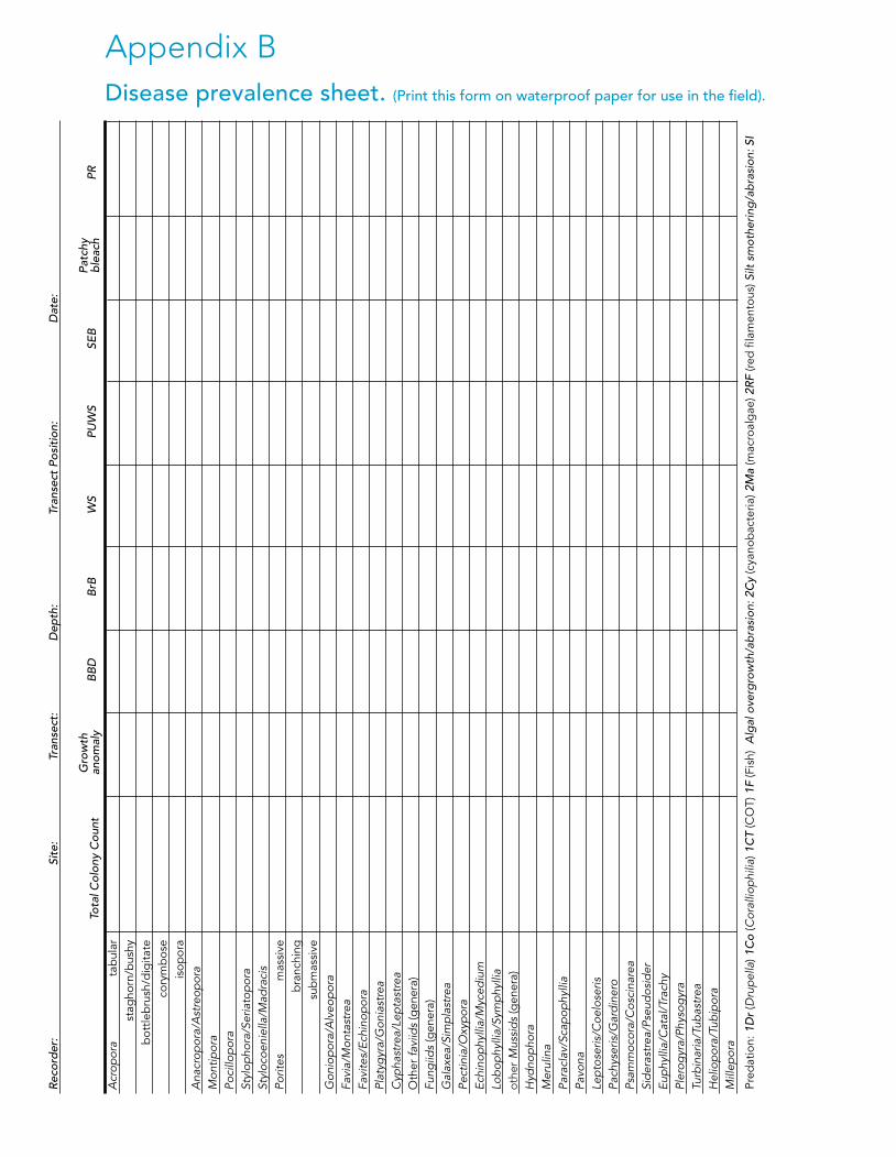
CRTR - Standard operating proceduresAppendix BDisease prevalence sheet. (Print this form on waterproof paper for use in the field).

Acr

opor

a

tab

ular

st

agho

rn/b

ushy

b

ottle

bru

sh/d

igita

te

cory

mb

ose

is

opor

aA

nacr

opor

a/A

stre

opor

aM

ontip

ora

Poci

llop

ora

Styl

opho

ra/S

eria

top

ora

Styl

ocoe

niel

la/M

adra

cis

Porit

es

mas

sive

b

ranc

hing

su

bm

assi

veG

onio

por

a/A

lveo

por

aFa

via/

Mon

tast

rea

Favi

tes/

Echi

nop

ora

Plat

ygyr

a/G

onia

stre

aC

ypha

stre

a/Le

pta

stre

aO

ther

favi

ids

(gen

era)

Fung

iids

(gen

era)

Gal

axea

/Sim

pla

stre

aPe

ctin

ia/O

xyp

ora

Echi

nop

hylli

a/M

yced

ium

Lob

ophy

llia/

Sym

phy

llia

oth

er M

ussi

ds

(gen

era)

Hyd

nop

hora

Mer

ulin

aPa

racl

av/S

cap

ophy

llia

Pavo

naLe

pto

seris

/Coe

lose

risPa

chys

eris

/Gar

din

ero

Psam

moc

ora/

Cos

cina

rea

Sid

eras

trea

/Pse

udos

ider

Eup

hylli

a/C

atal

/Tra

chy

Pler

ogyr

a/Ph

ysog

yra

Turb

inar

ia/T

ubas

trea

Hel

iop

ora/

Tub

ipor

aM

illep

ora

Pred

atio

n: 1

Dr

(Dru

pel

la) 1

Co

(Cor

allio

phi

lia) 1

CT

(CO

T) 1

F (F

ish)

Alg

al o

verg

row

th/a

bra

sion

: 2C

y (c

yano

bac

teria

) 2M

a (m

acro

alg

ae) 2

RF

(red

fila

men

tous

) Silt

sm

othe

ring

/ab

rasi

on: S

I

Rec

ord

er:

Site

: Tr

anse

ct:

Dep

th:

Tr

anse

ct P

osit

ion:

D

ate:

Tota

l Col

ony

Cou

nt

G

row

th

anom

aly

Patc

hy

ble

ach

BB

DB

rBW

SPU

WS

SEB

PR

29

Appendix BDisease prevalence sheet. (Print this form on waterproof paper for use in the field).

appendices

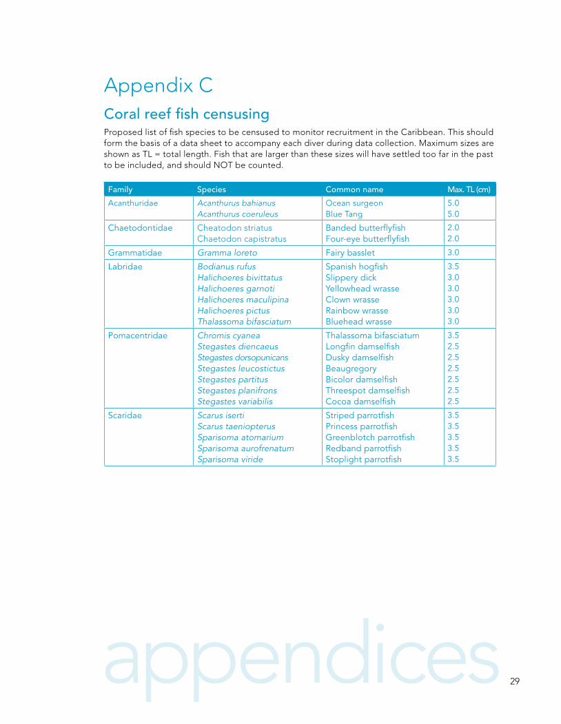
Appendix CCoral reef fish censusingProposed list of fish species to be censused to monitor recruitment in the Caribbean. This should form the basis of a data sheet to accompany each diver during data collection. Maximum sizes are shown as TL = total length. Fish that are larger than these sizes will have settled too far in the past to be included, and should NOT be counted.

Family Species Common name Max. TL (cm)

Acanthuridae Acanthurus bahianus Acanthurus coeruleus

Ocean surgeon Blue Tang

5.0 5.0

Chaetodontidae Cheatodon striatus Chaetodon capistratus

Banded butterflyfish Four-eye butterflyfish

2.0 2.0

Grammatidae Gramma loreto Fairy basslet 3.0

Labridae Bodianus rufus Halichoeres bivittatus Halichoeres garnoti Halichoeres maculipina Halichoeres pictus Thalassoma bifasciatum

Spanish hogfish Slippery dick Yellowhead wrasse Clown wrasse Rainbow wrasse Bluehead wrasse

3.5 3.0 3.0 3.0 3.0 3.0

Pomacentridae Chromis cyanea Stegastes diencaeus Stegastes dorsopunicans Stegastes leucostictus Stegastes partitus Stegastes planifrons Stegastes variabilis

Thalassoma bifasciatum Longfin damselfish Dusky damselfish Beaugregory Bicolor damselfish Threespot damselfish Cocoa damselfish

3.5 2.5 2.5 2.5 2.5 2.5 2.5

Scaridae Scarus iserti Scarus taeniopterus Sparisoma atomarium Sparisoma aurofrenatum Sparisoma viride

Striped parrotfish Princess parrotfish Greenblotch parrotfish Redband parrotfish Stoplight parrotfish

3.5 3.5 3.5 3.5 3.5


30 appendices

Appendix C cont...Date Site Observer Time

Species Common name TL Trans Trans Trans Trans

Acanthurus bahianus Ocean surgeon 5

A. coeruleus Blue Tang 5

Chaetodon striatus Banded butterfly 2

C. capistratus Four-eye butterfly 2

Gramma loreto Fairy basslet 3

Bodianus rufus Spanish hogfish 3.5

Halichoeres bivittatus Slippery dick 3

Halic. garnoti Yellowhead wras 3

Halic. maculipinna Clown wrasse 3

Halic. pictus Rainbow wrasse 3

Thalassoma bifasciatum Bluehead wrasse 3

Chromis cyanea Blue chromis 3.5

Stegastes diencaeus Longfin damsel 2.5

Steg. dorsopun Dusky damselfish 2.5

Steg. leucost Beaugregory 2.5

Steg. partitus Bicolor damselfish 2.5

Steg. planifrons Threespot damsel 2.5

Steg. variabilis Cocoa damselfish 2.5

Scarus iserti Striped parrotfish 3.5

Sc. taeniopterus Princess parrot 3.5

Scarus vetula Queen parrotfish 3.5

Spar. aurofren Redband parrotfish 3.5

Spar. viride Stoplight parrotfish 3.5

31appendices

Appendix D Taxonomic Amalgamation Units (TAUs)It is often very difficult and at times impossible to identify certain scleractinian corals to species level, even for a trained and experienced eye. Because of these challenges and the additional challenges associated with identifying from photos, Taxonomic Amalgamation Units were developed. All four geographic regions use these TAUs, These regions, and their TAUs should be used by all future programs to ensure that comparisons can be made with the current program. Note: The species list given here is not exhaustive (because there are hundreds more coral species, globally); therefore the species list will expand within each TAU as monitoring is initiated in other regions.

*The TAU ID (Name) is provided with the associated species listed below each TAU.

1. Pocillopora damicornis a. Pocillopora damicornis

2. Pocillopora verrucosa a. Pocillopora verrucosa

3. Stylophora spp. a. Stylophora spp.

4. Seriatopora spp. a. Seriatopora spp.

5. Isopora (Acropora) a. Acropora palifera b. Acropora cuneata c. Acropora brueggemanni

6. Acropora corymbose a. Acropora gemmifera b. Acropora humilis c. Acropora nasuta d. Acropora cerealis e. Acropora divaricata f. Acropora glauca g. Acropora valida h. Acropora digitifera i. Acropora secale j. Acropora verweyi k. Acropora monticulosa l. Acropora samoensis m. Acropora subulata n. Acropora tenuis o. Acropora donei p. Acropora selago q. Acropora polystoma r. Acropora selago s. Acropora donei t. Acropora anthocercis u. Acropora millepora v. Acropora samentosa w. Acropora microclados x. Acropora latistella

7. Acropora branching a. Acropora muricata (formosa) b. Acropora forskali c. Acropora intermedia (nobilis) d. Acropora microphthalma e. Acropora striata f. Acropora yongei g. Acropora aspera h. Acropora pulchra i. Acropora grandis j. Acropora austera k. Acropora palmata l. Acropora cervicornis

8. Acropora table a. Acropora cytherea b. Acropora clathrata c. Acropora hyacinthus d. Acropora paniculata

9. Acropora ‘hispidose’ a. Acropora echinata b. Acropora batunai c. Acropora subglabra d. Acropora carduus e. Acropora awi f. Acropora elseyi g. Acropora longicyathus h. Acropora turaki

10. Acropora robusta group a. Acropora danai b. Acropora robusta c. Acropora abrotanoides

11. Montipora foliose a. Montipora aequituberculata b. Montipora foliosa c. Montipora cebuensis d. Montipora capricornis e. Montipora crassituberculata


32 appendices

Appendix D cont...

12. Montipora encrusting a. Montipora efflorescens b. Montipora grisea c. Montipora hoffmeisteri d. Montipora informis e. Montipora millepora f. Montipora tuberculosa g. Montipora undata h. Montipora venosa i. Montipora verrucosa

13. Montipora branching a. Montipora digitata b. Montipora gaimardi c. Montipora hispida d. Montipora cactus

14. Porites massive a. Porites lobata b. Porites lutea c. Porites astreoides

15. Porites branching a. Porites annae b. Porites cylindrica c. Porites nigrescens d. Porites profundus e. Porites negrosensis f. Porites samarensis g. Porites porites h. Porites furcata i. Porites divaricata

16. Porites encrusting a. Porites aranetai b. Porites rus c. Porites branneri

17. Favites spp. a. Favites abdita b. Favites chinensis c. Favites complanata d. Favites flexuosa e. Favites halicora f. Favites pentagona g. Favites russelli h. Favites vasta

18. Goniastrea spp. a. Goniastrea aspera b. Goniastrea australensis c. Goniastrea edwardsi d. Goniastrea pectinata e. Goniastrea peresi f. Goniastrea retiformis

19. Montastrea spp. a. Montastrea spp. b. Montastrea annularis c. Montastrea cavernosa d. Montrastrea faveolata e. Montastrea franksi

20. Favia spp. a. Favia favus b. Favia helianthoides c. Favia laxa d. Favia lizardensis e. Favia maritima f. Favia pallida g. Favia rotumana h. Favia speciosa i. Favia stelligera j. Favia veroni k. Favia fragum l. Favia gravida m. Favia leptophylla

21. Leptoria spp. a. Leptoria phrygia b. Leptoria irregularis

22. Platygyra spp. a. Platygyra crosslandi b. Platygyra daedalea c. Platygyra lamellina d. Platygyra sinensis e. Platygyra pini

23. Lobophyllia spp. a. Lobophyllia corymbosa b. Lobophyllia hataii c. Lobophyllia hemprichii d. Lobophyllia robusta

24. Galaxea spp. a. Galaxea astreata b. Galaxea fascicularis

25. Symphyllia spp. a. Symphyllia agaricia b. Symphyllia recta c. Symphyllia radians

26. Fungia spp. a. Fungia spp.

27. Goniopora spp. a. Goniopora spp.

33appendices

28. Encrusting other a. Pavona explanulata b. Pavona minuta c. Pavona bipartita d. Cyphastrea microphthalma e. Acanthastrea hemprichii f. Coscinaraea monile g. Cyphastrea chalcidium h. Agaricia humilis i. Dendrogyra cylindrus j. Madracis pharensis

29. Massive other a. Caulastrea furcata b. Caulastrea tumida c. Acanthastrea lordhowensis d. Alveopora fenestrata e. Alveopora tizardi f. Astreopora myriophthalma g. Coeloseris mayeri h. Cyphastrea serailia i. Diploastrea heliopora j. Echinophyllia orpheensis k. Gardineroseris planulata l. Oulophyllia crispa m. Colpophyllia natans n. Dichocoenia stokesi o. Diploria clivosa p. Diploria labyrinthiformis q. Diploria strigosa r. Eusmilia fastigiata s. Isophyllastrea rigida t. Isophyllia sinuosa u. Manicina areolata v. Meandrina meandrites w. Mussa angulosa x. Mussismilia braziliensis y. Mussismilia harttii z. Mussismilia hispida aa. Siderastrea radians bb. Siderastrea siderea cc. Siderastrea stellata dd. Solenastrea bournoni ee. Solenastrea hyades ff. Stephanocoenia intersepta gg. Scolymia cubensis

30. Turbinaria spp. a. Turbinaria spp.

31. Foliose-plates a. Pavona cactus b. Astreopora expansa c. Echinophyllia echinata d. Mycedium mancaoi e. Echinopora lamellosa f. Pavona varians g. Pavona decussata h. Psammocora superficialis i. Coscinaraea crassa j. Echinophyllia aspera k. Podabacia motuporensis l. Psammocora contigua m. Agaricia agaricites n. Agaricia tenuifolia o. Agaricia fragilis p. Agaricia grahamae q. Agaricia lamarcki r. Agaricia undata s. Mycetophyllia aliciae t. Mycetophyllia danaana u. Mycetophyllia ferox v. Mycetophyllia lamarckiana w. Porites colonensis x. Scolymia lacera y. Leptoseris cucullata

32. Branching other a. Oculina diffusa b. Oculina varicose c. Cladacora arbuscula d. Madracis decactis e. Madracis formosa f. Madracis mirabilis


34 references

References

1. Bak P.M & Meesters E.H. (1999) Population structure as a response of coral communities to global change. American Zoologist 39: 56-65.

2. Brown, B.E. (1997) Coral bleaching: causes and consequences. Coral Reefs 16, 129-138.

3. Condit et R, Sukumar R, Hubbell SP, Foster RB (1998) Predicting population trends from size distributions: a direct test in a tropical tree community. American Naturalist 152: 495-509.

4. Darwin, C. 1842. The structure and distribution of coral reefs. London.

5. Dethier, M. N., E. S. Graham, et al. 1993. Visual versus random-point percent over estimations: ‘objective’ is not always better. Marine Ecology Progress Series 96:93 100.

6. Glynn, P.W. (1991) Coral reef bleaching in the 1980s and possible connections with global warming. Trends in Ecology and Evolution 6, 175-179.

7. Green R, McArdle B, van Woesik R (Submitted) Sampling state and process variables on coral reefs. Environmental Monitoring and Assessment.

8. Hoegh-Gulberg, O. (1999) Climate change, coral bleaching and the future of the world’s coral reefs. Marine Freshwater Research 50 (8), 839-866.

9. Loya Y, Sakai K, Yamazato K, Nakano H, Sambali H, Van Woesik R (2001) Coral bleaching: the winners and the losers. Ecology Letters 4:122-131.

10. Nakamura T, Van Woesik R (2001) Water-flow rates and passive diffusion partially explain differential survival of corals during 1998 bleaching event. Marine Ecology Progress Series 212: 301-304.

11. Raymundo, L.J., C.S. Couch and C. D.Harvell, (Eds) 2007. Coral Disease Handbook: Coral Disease Handbook: Guidelines for Assessment Monitoring and Management 121 pp.

12. Rogers, C.S.; Garrison, G.; Grober, R.; Hillis, Z.-M. and Franke, M.A. (2001). Coral Reef Monitoring Manual for the Caribbean and Western Atlantic. St John, U.S. Virgin Islands. 107 pp.

13. Vidondo B, Prairie YT, Blanco JM, Duarte CM (1997) Some aspects of the analysis of size spectra in aquatic ecology. Limnology and Oceanography 42(1): 184-192.

14. Zvuloni A, Artzy-Randrup Y, Stone L, van Woesik R, Loya Y (2008) Ecological size-frequency distributions: how to prevent and correct biases in spatial sampling. Limnology & Oceanography 6: 144-153.

notes

Notes

Standard Operating Proceduresfor Repeated Measures of Process and State Variables

The CRTR Program is a partnership between the Global Environment Facility, the World Bank, The University of Queensland (Australia), the United States National Oceanic and Atmospheric Administration (NOAA) and approximately 50 research institutes and other third-parties around the world.

Documents

Standard Operating Procedures - Coral Reef Targeted Research