REVIEW ARTICLE

Standard methods for molecular research in Apis

mellifera

Jay D Evans1*, Ryan S Schwarz1, Yan Ping Chen1, Giles Budge2, Robert S Cornman1, Pilar De la Rua3,

Joachim R de Miranda4, Sylvain Foret5, Leonard Foster6, Laurent Gauthier7, Elke Genersch8 ,

Sebastian Gisder8, Antje Jarosch9, Robert Kucharski5, Dawn Lopez1, Cheng Man Lun10, Robin F A Moritz9, Ryszard Maleszka5, Irene Muñoz3 and M Alice Pinto11 1USDA-ARS, Bee Research Lab, BARC-E Bldg 306, Beltsville MD 20705, USA. 2National Bee Unit, Food and Environment Research Agency, Sand Hutton, York, YO41 1LZ, UK. 3Department of Zoology and Physical Anthropology, Faculty of Veterinary, University of Murcia, Spain. 4Department of Ecology, Swedish University of Agricultural Sciences, Uppsala, 750-07, Sweden. 5Research School of Biology, The Australian National University, Australia Australian National Univ. Canberra, ACT 0200, Australia. 6Centre for High Throughput Biology, University of British Columbia, Vancouver, BC, Canada. 7Swiss Bee Research Centre, Agroscope Liebefeld-Posieux Research Station ALP, Bern, CH-3003, Switzerland. 8Institute for Bee Research, Friedrich-Engels-Str. 32, 16540 Hohen Neuendorf, Germany. 9Martin-Luther-University Halle-Wittenberg, Dept. of Biology, Molecular Ecology, Hoher Weg 4, 06099 Halle, Germany. 10George Washington University, Department of Biological Sciences, Lisner Hall 340, 20234 G St. NW, Washington, DC 20052, USA. 11Mountain Research Centre (CIMO), Polytechnic Institute of Bragança, Bragança, Portugal. Received 19 March 2012, accepted subject to revision 25 September 2012, accepted for publication 11 February 2013. *Corresponding author: Email: jay.evans@ars.usda.gov

Summary

From studies of behaviour, chemical communication, genomics and developmental biology, among many others, honey bees have long been a

key organism for fundamental breakthroughs in biology. With a genome sequence in hand, and much improved genetic tools, honey bees are

now an even more appealing target for answering the major questions of evolutionary biology, population structure, and social organization.

At the same time, agricultural incentives to understand how honey bees fall prey to disease, or evade and survive their many pests and

pathogens, have pushed for a genetic understanding of individual and social immunity in this species. Below we describe and reference tools

for using modern molecular-biology techniques to understand bee behaviour, health, and other aspects of their biology. We focus on DNA and

RNA techniques, largely because techniques for assessing bee proteins are covered in detail in Hartfelder et al. (2013). We cover practical

needs for bee sampling, transport, and storage, and then discuss a range of current techniques for genetic analysis. We then provide a

roadmap for genomic resources and methods for studying bees, followed by specific statistical protocols for population genetics, quantitative

genetics, and phylogenetics. Finally, we end with three important tools for predicting gene regulation and function in honey bees:

Fluorescence in situ hybridization (FISH), RNA interference (RNAi), and the estimation of chromosomal methylation and its role in epigenetic

gene regulation.

Journal of Apicultural Research 52(4): (2013) © IBRA 2013 DOI 10.3896/IBRA.1.52.4.11

Footnote: Please cite this paper as: EVANS, J D; SCHWARZ, R S; CHEN, Y P; BUDGE, G; CORNMAN, R S; DE LA RUA, P; DE MIRANDA, J R; FORET, S; FOSTER, L; GAUTHIER, L; GENERSCH, E; GISDER, S; JAROSCH, A; KUCHARSKI, R; LOPEZ, D; LUN, C M; MORITZ, R F A; MALESZKA, R; MUÑOZ, I; PINTO, M A (2013)

Standard methodologies for molecular research in Apis mellifera. In V Dietemann; J D Ellis; P Neumann (Eds) The COLOSS BEEBOOK, Volume I: standard methods for Apis mellifera research. Journal of Apicultural Research 52(4): http://dx.doi.org/10.3896/IBRA.1.52.4.11

2 Evans et al.

Métodos estándar para la investigación molecular en Apis

mellifera

Resumen

Las abejas de miel han sido durante mucho tiempo un organismo clave para avances fundamentales en biología a partir de estudios de su

comportamiento, comunicación química, genómica y de biología del desarrollo, entre otros muchos. Con la secuencia del genoma en la mano

y herramientas genéticas mucho mejores, las abejas son ahora un blanco aún más atractivo para responder a las preguntas más importantes

de la biología evolutiva, la estructura de las poblaciones y la organización social. Al mismo tiempo, los incentivos agrícolas para entender cómo

las abejas caen enfermas, o evadir y sobrevivir a sus muchas plagas y patógenos, han presionado para comprender genéticamente la

inmunidad individual y social en esta especie. A continuación se describen y se hace referencia a herramientas que hacen uso de modernas

técnicas de biología molecular para entender el comportamiento de las abejas, su salud y otros aspectos de su biología. Nos centramos en las

técnicas de ADN y ARN, en gran parte debido a que las técnicas de evaluación de las proteínas de la abeja se tratan en detalle en Hartfelder

et al. (2013). Cubrimos las necesidades prácticas de toma de muestras de abejas, su transporte y almacenamiento, y luego se discuten una

serie de técnicas actuales de análisis genético. A continuación, se proporciona una hoja de ruta para los recursos genómicos y métodos para

estudiar las abejas, seguido de protocolos estadísticos específicos de la genética de poblaciones, la genética cuantitativa y la filogenia.

Finalmente, se termina con tres herramientas importantes para predecir la regulación génica y la función en las abejas melíferas: la

hibridación in situ fluorescente (FISH), la interferencia de ARN (iARN), y la estimación de la metilación cromosómica y su papel en la

regulación epigenética de los genes.

西方蜜蜂分子研究的标准方法

摘要

通过行为、化学通讯、基因组和发育生物学等方面的研究，蜜蜂已经成为用于在生物学基础研究领域取得重大突破的一种重要模式生物。结合已

有的基因组序列和多种改进的遗传学工具，蜜蜂已经越加成为回答进化生物学、种群结构和社会性结构等方面重大问题极具吸引力的研究目标。

与此同时，农业上为了解蜜蜂如何困于病害或者避开和幸存于多种害虫和病原菌的危害，也促进了对这一物种个体和社会免疫的遗传学理解。以

下我们介绍和引用了一些运用现代分子生物学技术研究蜜蜂行为、健康、以及其它方面生物学的工具。Hartfelder等2013已对研究蜜蜂蛋白做了

详细的论述，因此我们将重点放在DNA和RNA技术上。本文也包含了在蜜蜂采样、运输和保存过程中的实际需要，并讨论了当前的一系列遗传分

析技术。然后我们提供了研究蜜蜂时所需的基因组资源和方法的路线图，以及群体遗传学、数量遗传学和系统发生学研究中特定的统计学方法。

最后，我们以预测蜜蜂基因调控和功能的三个重要工具收尾：荧光原位杂交（FISH）、RNA干扰（RNAi）和染色体甲基化及其在表观遗传基因

调控中作用的估算。

Keywords: Apis mellifera, pollination, disease, development, genomic, Colony Collapse Disorder, population genetics, methylation, RNA

interference, RNAi, Southern Blot, Northern Blot, In situ Hybridization, DNA extraction, Next-generation sequencing, mitochondrial DNA,

microsatellite, quantitative PCR, COLOSS, BEEBOOK, honey bee

The COLOSS BEEBOOK: molecular methods 3

Page No.

4. RNA methods 14

4.1. Introduction 14

4.2. Affinity column purification 14

4.3. Acid Phenol RNA extraction from adult bees 15

4.3.1. TRIzol extraction 15

4.3.2. Bulk Extraction of RNA from 50-100 whole bees using the acid-phenol method

16

4.3.3. RNA lysis/stabilization buffer 17

4.4. RNA quality assessment 17

4.5. cDNA synthesis from total RNA 17

4.5.1. Reverse Transcription of RNA 17

4.6. Qualitative RT-PCR for honey bee and pathogen targets 18

4.7. Quantitative RT-PCR for honey bee and pathogen targets

18

4.7.1. One-Step versus Two-Step RT-PCR 19

4.7.2. One-Step RT-qPCR 19

4.7.3. Two-Step RT-qPCR 19

4.7.4. Two-step Quantitative PCR for high-throughput assays 19

4.7.5. Multiplex RT-(q)PCR 20

4.8. Primer and probe design 20

4.8.1. Primer length, melting temperature and composition 20

4.8.2. Annealing temperature 20

4.8.3. Cycling parameters 21

4.9. Assay optimization 21

4.9.1. Primer-dimers and other PCR artefacts 21

4.9.2. Primer concentration 21

4.9.3. Magnesium concentration 21

4.10 Quantitation controls 21

4.10.1. External reference standards 21

4.10.2. Internal reference standards 23

4.10.2.1. Exogenous internal reference standards 23

4.10.2.2. Internal reference standards 23

4.10.2.3. External standard for viral target quantification 24

4.11. Microarrays 24

4.12. Northern blots using DIG labelling 24

4.12.1. Agarose / Formaldehyde gel electrophoresis 24

4.12.2. Assembly of the transfer setup and transfer of RNA from gel to membrane

25

4.12.3. Preparation of DIG labelling (non-radioactive) probe 25

4.12.4. Hybridization analysis 26

4.13. In situ hybridization 26

4.13.1. Tissue fixation 26

4.13.2. Preparation of DIG labelling (non-radioactive) probe 26

4.13.3. Hybridization analysis

26

5. Proteomic methods

27

5.1. Introduction 27

6. Population genetics

27

Table of Contents Page No.

1. Sample management 5

1.1. Introduction 5

1.2. Sample collection 5

1.2.1. Adult bees 5

1.2.1.1. Nurse bees 5

1.2.1.2. Foraging bees

5

1.2.2. Pupae 5

1.2.3. Larvae 5

1.2.4. Eggs 5

1.2.5. Extracted guts 6

1.2.6. Drone endophalus and semen 6

1.2.7. Faeces

6

1.2.8. Dead bee samples 6

1.3. Sample transport 6

1.3.1. Freezing with dry ice 6

1.3.2. Freezing with “wet” ice 6

1.3.3. Live transport 7

1.3.4. Chemical stabilizers 7

1.3.5. Sample collection cards 8

1.4. Long-term sample storage 8

1.4.1. Freezing 8

1.4.2. Drying 8

1.4.3. Chemical stabilizers 8

2. Sample processing 9

2.1. Introduction 9

2.2. Sample homogenization 9

2.2.1. Bead-mill homogenizers 9

2.2.2. Blender 9

2.2.3. Paint shaker 9

2.2.4. Mortar and pestle 9

2.2.5. Mesh bags 10

2.2.6. Micropestle 10

2.2.7. Robotic extraction 10

3. DNA extraction and analysis 10

3.1. Introduction

10

3.2. Genomic DNA extraction from adult bees 10

3.2.1. DNA extraction using CTAB 10

3.2.2. DNA extraction using Qiagen Blood and Tissue DNA kits 12

3.2.3. DNA extraction using Chelex 12

3.3. DNA detection using southern blots with DIG labelling 12

3.3.1. Restriction enzyme digestion and agarose gel electrophoresis

12

3.3.2. Assembly of the transfer setup and transfer of DNA from gel to membrane

13

3.3.3. Synthesis of DIG-labelled DNA probe 13

3.3.4. Hybridizing the DIG-labelled DNA Probe to DNA on the Blot

13

4 Evans et al.

Table of Contents cont’d Page No.

6.1. Introduction 27

6.2. Mitochondrial DNA analysis 27

6.3. Nuclear DNA analysis 28

6.3.1. Microsatellites

28

6.3.1.1. Microsatellite reaction mix 28

6.3.1.2. Primers for multiplexed honey bee microsatellite loci

29

6.3.1.3. Thermal cycling conditions for multiplex PCR 29

6.3.1.4. Size estimation of PCR products 29

6.3.2. Single-nucleotide polymorphisms (SNPs) 29

7. Phylogenetic analysis of sequence data 30

7.1. Introduction 30

7.2. Obtaining and formatting sequences of interest for phylogenetics

30

7.3. Sequence data in FASTA format 30

7.4. Alignment of sequence data 31

7.4.1. Clustal 31

7.4.2. MUSCLE 31

7.5. Trimming aligned sequence data to equal length

31

7.6. Performing phylogenetic analyses 31

7.6.1. Using MEGA 31

7.6.1.1. Converting data to MEGA format 32

7.6.1.2. Constructing and testing phylogenetic trees 32

7.6.2. Using SATé

33

7.6.2.1. External tools 33

7.6.2.2. Sequence import and tree building 33

7.6.2.3. Job Settings 33

7.6.2.4. SATé Settings 33

7.6.3. Building trees using distance and character based methods

33

8. Genomic resources and tools

34

8.1. Introduction 34

8.2. Honey bee genome project 34

8.3. Honey bee parasite and pathogen genomes 34

8.4. Comparative genomics

34

8.5. Second-generation sequencing 35

8.6. Genomic sequence assembly 35

8.7. Transcriptomic analyses (“RNASeq”) 35

8.8. Metagenomics 35

8.8.1. RNA versus DNA sampling 35

8.8.2. Sample preparation 36

8.8.3. Amplicon-based or shotgun sequencing 36

Page No.

8.8.4. Assembly of shotgun sequences vs. read mapping 36

8.8.5. Databases for metagenomics 36

8.8.6. Post-assignment statistics 36

9. Fluorescence in situ hybridization (FISH) analysis of tissues and cultured cells

37

9.1. Introduction 37

9.2. Tissue fixation and tissue sectioning exemplified with gut tissue

37

9.3. Fixation of cultured cells grown in suspension 37

9.4. FISH-analysis of tissue sections and fixed insect cells 37

10. RNA Interference 38

10.1. Introduction 38

10.2. Production of RNA interfering molecules 38

10.2.1. siRNA design and synthesis

38

10.2.2. Production of dsRNA 39

10.3. RNAi Applications 40

10.3.1. RNAi in adult honey bees via feeding 40

10.3.2. RNAi in honey bee larvae via feeding 40

10.3.3. Gene knock-down by abdominal injection of target-specific dsRNA/siRNA

40

10.4. Concluding remarks 40

11. DNA methylation in honey bees 41

11.1. Introduction 41

11.2. DNA methylation in honey bees 41

11.3. DNA extraction from various tissues for methylation analysis

41

11.4. High-throughput sequencing of targeted regions 42

11.4.1. Fragmentation of DNA 42

11.4.2. End-repair of sheared DNA 42

11.4.3. Adaptor ligation 42

11.4.4. Size selection of adapter-ligated fragments

42

11.4.5. Bisulfite conversion and amplification of the final library

42

11.4.6. Validation of the libraries 42

11.4.7. Sequencing and data analysis 42

11.5. Mapping and methylation assessment 42

11.6. Methylation dynamics and expression of individual genes

43

11.6.1. Amplicon sequence selection 43

11.6.2. Bisulfite DNA conversion 43

11.6.3. Bisulfite PCR 43

11.7. RNA extraction 44

11.8. cDNA synthesis and template quantification 44

12. Acknowledgements 44

13. References 44

1. Sample management

1.1. Introduction

In order to best reflect honey bee biology, data generated from

molecular-genetic studies should reflect as closely as possible the

state of honey bee tissues, entire bees, or colonies just prior to

sampling. This fact places a premium on collecting and storing

samples in a way that retains this state. Although technological

developments in molecular biology allow for a great diversity of

insights from collected bee samples, it is often forgotten how much

these insights are hampered by errors in the collection, storage and

processing of samples (Chernesky et al., 2003). These problems are

especially evident when data from different studies or laboratories are

compared (Birch et al., 2004). The only solution to this is optimization

of collection, storage and primary processing protocols, so as to

minimize the influence of sample degradation on the molecular

analyses and the reliability of the data. As is often the case, cues can

be taken from other areas of biology, notably the medical field, where

such practices are widely adopted (Valentine-Thon et al., 2001;

Verkooyen et al., 2003).

A secondary consideration is that a sample may be used for

several different analyses; proteins, nucleic acids, fats and lipids,

metabolites etc., requiring a collection and processing protocol

suitable for all compounds analysed. Usually this means that the

sample management conditions follow the requirements for the least

stable of the compounds, which for bee research is usually the RNA.

RNA is highly sensitive to degradation by robust RNAse enzymes

found in all cells, unless the sample is stabilized with RNAse-inhibiting

additives and/or frozen as soon as possible. Given the necessity of

RNA analyses for many questions related to bees and their parasites

and pathogens (e.g., de Miranda et al. 2013), field-appropriate

methods for stabilizing RNA are required.

1.2. Sample collection

The optimum strategy for collection and transport of bee samples

depends partly on what type of sample is collected. Bees, pupae,

larvae and eggs can be sampled whole or as field-dissected

components, such as heads, thoraxes, abdomens, guts, endophalli,

semen, ovaries etc. Many bee viruses are shed in large amounts in

the guts, as are many bacterial and protozoan pathogens (Shimanuki,

1997; Fries, 1997). Faeces may therefore be a good marker for the

infection status of the whole bee, although care has to be taken to

distinguish between passively acquired/passaged microbes and true

tissue infections. Faeces also allow bees to be sampled repeatedly, and

non-destructively. It may therefore be useful for determining the virus

status of queens (Hung, 2000), especially if these are a major source

of infection of the worker population (Chen et al., 2005b; Fievet et al.,

2006), or for following disease progression in individual bees.

5

Below are suggestions for the collection of different types of bee

samples. In all cases a priori decisions are all needed with respect to

the use of chemical stabilizers, collection cards and the temperatures

during transport and storage.

1.2.1. Adult bees

1.2.1.1. Nurse bees

Inspect each frame in a colony and find a frame with sealed and

unsealed brood which is covered by adhering nurse bees and then

take the frame out of the colony.

1.2.1.2. Foraging bees

Block the hive entrance where foraging bees are accumulating and

collect the returning foraging bees.

1.2.2. Pupae

1. Cut out a section of sealed brood, to be transported whole.

Such a brood section can be sent through the post, although

with the caveat that such transport away from the hive might

affect bee or parasite gene activities.

2. Uncap brood cells, lift pupae by their neck by curling fine

curved forceps underneath their heads and transfer to a

suitable transport medium, either individual microcentrifuge

tubes or collection cards (see section 1.3.5).

1.2.3. Larvae

1. Cut out a section of open brood and transport in a

temperature -humidity controlled box, to prevent dehydration.

2. Remove larvae from the comb using either a blunt grafting

needle (small larvae) or soft forceps (large larvae) and

transfer to individual microcentrifuge tubes or collection cards.

1.2.4. Eggs

1. Cut out a section of comb with eggs and transport in a

temperature-humidity controlled box, to prevent dehydration.

2. Remove eggs using a blunt needle and transfer individually or

in bulk to microcentrifuge tubes or collection cards.

As an alternative for the rapid collection of massive amounts of eggs

and early embryos:

1. Strike soundly a frame containing early-stage bees onto a

sterile surface twice.

This releases over half of the eggs and embryos held by that frame,

2. Brush or lift into a new vessel.

While uncapped honey will drip via this method, if done at the right

intensity, older uncapped larvae will remain in their cells.

The COLOSS BEEBOOK: molecular methods

1.2.5. Extracted guts

1. Grab the stinger and last integument of adult worker bees

firmly with a pair of fine, straight forceps.

2. Pull backwards gently, removing the whole hindgut and

midgut.

3. Transfer guts to individual microcentrifuge tubes or collection

cards (see section 1.3.5.).

1.2.6. Drone endophallus and semen

1. Turn drone upside down and grip laterally between thumb

and index finger.

2. With the other hand, gently but persistently squeeze the

abdomen of the drone dorso-ventrally, exerting pressure

backwards, until the endophallus is extruded from the drone.

3. Apply more severe pressure, again backwards, to avert the

endophallus and, for mature drones, cause ejaculation of

semen.

4. Cut off the entire endophallus with scissors, or collect the

exposed semen (brown-red colour) and/or seminal fluid

(translucent white) with a sterile micropipette.

5. Collect the material individually in microcentrifuge tubes or on

collection cards.

1.2.7. Faeces

If destructive sampling is allowed:

1. Remove the whole gut from individual bees (see above) and

expel faecal mass.

If repeated sampling is required:

1. Place adult bees into a Petri dish until defecation has

occurred.

2. Collect faeces individually or pooled in microcentrifuge tubes

or on collection cards.

1.2.8. Dead bee samples

Many bee disease experiments involve bee death as a parameter.

Dead bee samples from such experiments are, of course, valid

material for analysis. They should be treated like freshly killed material

and frozen as soon as possible to minimize the effects of decay on

RNA integrity, using the collection methods appropriate for the sample

type, as given above. Dead bee traps attached to hives are suitable

for collecting such bees and should be emptied daily to minimize the

effects of decomposition.

Passive surveys also involve dead bee samples, in this case those

sent in by beekeepers for post-mortem analysis of the cause of colony

death. These bees will have been dead long enough for decomposition

and drying to have severely affected the integrity of the RNA, including

viral RNAs. Such degradation can severely affect the accuracy and

reliability of detecting and quantifying individual RNAs (Bustin and

Nolan, 2004; Fleige and Pfaffl, 2006; Becker et al., 2010). This means

6 Evans et al.

that only positive results from such samples are informative, since

negative results can be either due to the absence of virus or the

degradation of the RNA.

It is possible to adjust for differential RNA degradation in the

different samples with quantitative RT-qPCR techniques, by using host

internal reference gene levels for normalizing the virus titers (Dainat

et al., 2011) and setting the threshold for template detection with the

most degraded sample, so that all samples are evaluated by the same

degradation criteria. How to determine the detection thresholds using

RT-qPCR assays is covered in section 4.4.

1.3. Sample transport

Sample transport from the collection site to the laboratory is the most

critical step in sample management, since this is where the integrity

of the sample is most easily compromised (Chen et al., 2007). Sample

integrity can be preserved to different degrees with the following

methods, given in order of effectiveness. The gold standard for sample

collection and transport is to freeze on-site, but this is not always

possible. All alternatives are basically aimed at getting the samples as

quickly and conveniently as possible into a freezer, with minimum

degradation. The most useful tool for transporting frozen material is a

liquid nitrogen-based ‘dry shipper’, which is specifically developed and

approved for international shipment of biological samples at ultra-low

temperatures (-150oC). The best can hold these temperatures for

more than one week. Other options, for more local transport, are

(dry) ice-boxes and portable/car freezers. Courier and mail services

are less reliable, both with respect to the maintenance of temperature

and the duration of transport.

1.3.1. Freezing with dry ice

Samples: all.

Conditions: freeze instantly; keep frozen throughout transport

using blocks of dry ice in a cooler.

Transport: restricted transport; dry ice must be replenished

ca. every 48 hours.

Processing: transfer samples to freezer.

Pros: gold standard; fast.

Cons: very expensive; complex field operation.

1.3.2. Freezing with ‘wet’ ice

Short-term field-storage on ‘wet’ (frozen water or ice packs) ice is

cheap and very practical for many field-studies and surveys. The

samples should be frozen as soon as possible, ideally within hours,

and kept frozen continuously until RNA processing (a complete frozen

transport chain). If a complete frozen transport chain cannot be

guaranteed, then a chemical stabilizing agent (see section 1.3.4.)

should be used to prevent degradation of the RNA by RNAses, until

the samples enter a frozen transport chain. The most important rule

for RNA preservation is to keep the samples as cold as possible, as

long as possible and to avoid thawing the sample after it has been

frozen unless it is to extract RNA.

Samples: all.

Conditions: collect in freezer bags, store on wet ice.

Transport: cold transport; wet-ice; < 12 hours.

Processing: transfer samples to freezer.

Pros: simple; fast; cheap field operation.

Cons: heavy, expensive mail transport, leaks due to

thawing.

1.3.3. Live transport

Bees can also be transported live, which allows them to be sent much

more quickly, cheaply and reliably by post than frozen samples. One

drawback is that the stress of live transport may affect the expression

of host genes, and possibly virus replication, which should be taken

into account when planning experiments.

1. Adult bees can be transported live 1) In a well-ventilated bee

shipping box containing queen candy and a sponge soaked in

water glued to the bottom of the box or 2) in units of 10-15

bees in commercial queen cages with queen candy. Such

queen cages are readily available to most beekeepers.

Samples: adults.

Conditions: room temperature.

Transport: < 48 hours.

Processing: freeze on arrival.

Pros: simple; fast; suitable for beekeepers.

Cons: stress during transport.

2. Pupae can be transported live 1) as a section of capped brood

in a well-ventilated bee shipping box, preferably in a warm

environment to prevent chilling, 2) as queen cells for queen

pupae in a specialized temperature-humidity controlled queen-

cell transport container, available from beekeeping suppliers.

Such cells should be handled with great care, as developing

queen pupae are very sensitive to disturbance, or 3) as a

whole frame in a specialized carrier box for frames, available

from beekeeping suppliers, or in a swarm box/nucleus hive.

Samples: pupae.

Conditions: room temperature.

Transport: < 48 hours.

Processing: remove samples from comb and freeze.

Pros: simple, fast.

Cons: pupae may emerge during transport.

3. Larvae and eggs can be transported live 1) as a section of

comb, in a temperature and humidity-controlled box or 2) as a

whole frame in a specialized carrier box for frames, or in a

swarm box/nuc.

The COLOSS BEEBOOK: molecular methods 7

Samples: larvae; eggs.

Conditions: controlled temperature and humidity.

Transport: less than 48 hours.

Processing: remove samples from comb and freeze.

Pros: simple, fast.

Cons: expensive by mail, unsealed larvae are subject to

temperature stress and starvation.

1.3.4. Chemical stabilizers

There are a number of chemicals that can be used to help stabilize

nucleic acids during transport. Their purpose is to inhibit nucleases,

especially the resilient RNAses, and in doing so destroy all enzymatic

activity in the sample. So, if the final assays include natural enzymatic

activity, these stabilizers should be avoided. For similar reasons, many

stabilizers are also incompatible with serological detection methods,

such as ELISA.

A large excess (5-fold by weight) of stabilizer should be added to

ensure a high enough concentration within the tissues for inhibiting

RNAses. It is also essential that the solution penetrates the tissues

completely to abolish all RNAse activity. This is a major difficulty for

aqueous stabilizers, which cannot penetrate the hydrophobic insect

exoskeleton. These are therefore only suitable for extracted tissues,

eggs and small larvae, unless bodies are partially disrupted at the

start. Organic preservatives, such as 100% ethanol, have much more

effective penetration of the exoskeleton and are therefore better for

stabilizing whole adult bee samples. Although 100% ethanol is

suitable for preserving RNA destined for short-fragment RT-qPCR-

based assays, storage in 70% ethanol has been shown to result in

strong degradation (Chen et al., 2007). However, recent data using a

short amplicon (124 bp) diagnostic for Deformed wing virus (DWV) in

a Taqman assay (Chantawannakul et al., 2006), showed no loss of

DWV signal after adult bees were stored for 4 weeks in 70% EtOH at

room temperature compared to snap frozen controls (G. Budge,

unpublished data). RNA can also be stabilized by high concentration

sulphate salt solutions (Mutter et al., 2004), of which RNAlater®

(Qiagen) is the best known. A generic version can be made as

follows:

700 g di-ammonium sulfate

40 ml 0.5M EDTA (pH 8.0)

25 ml 1M tri-sodium citrate (di-hydrate salt; 29.4 g/100 ml)

1l sterile water

~1.3 l total volume

Once stabilized, RNase activities will be inhibited and samples can

be stored for up to 1 month at 4°C, and long-term at -20°C or -80ºC

with minimal degradation. The stabilizer should be removed from the

bee sample prior to homogenization and RNA extraction.

1. 100% ethanol

Samples: whole adult bees; pupae; large larvae; tissues.

Use: 5 volumes by weight.

Storage: 1 month at room temperature or lower.

Processing: Remove ethanol and process samples as normal.

Pros: Cheap; effective penetration.

Cons: Evaporation; possible transport restrictions; heavy;

incompatible with serological assays .

2. RNAlater® & generic equivalent

Samples: tissues; eggs; small larvae.

Use: 5 volumes by weight.

Storage: 1 month at room temperature, or lower.

Processing: Remove stabilizer and process samples as normal.

Pros: Non-hazardous; effective penetration.

Cons: Expensive (except generic version); heavy.

It is possible to use RNAlater® for darkened pupae and adult

bees, if they are crushed into a paste or cut into 5mm sections (Chen

et al., 2007). This is laborious and risks losing virus particles and RNA

to the stabilizing solution, but may be required in certain circumstances.

In such cases, the crushed bees should be centrifuged at 1,000 rpm

for 5 minutes at 4oC before removing the stabilizer and processing the

crushed bee tissues.

1.3.5. Sample collection cards

Samples can also be dried on filter paper-based collection cards. In

this case the molecules are stabilized primarily through desiccation,

rather than low temperature, so thorough drying during sampling and

low humidity during storage is essential for this method. The FTA™-

cards produced by Whatman are furthermore impregnated with

chemicals to prevent bacterial or enzymatic degradation of nucleic

acids (Becker et al., 2004; Rensen et al., 2005). The method is ideal

for liquid samples (blood, urine, sputum etc.) but has also been used

for insect samples (Harvey, 2005) including honey bee larvae, pupae,

extracted tissues and mites. Such filter-dried samples can be analysed

for all manner of compounds (Jansson et al., 2003; Chamoles et al.,

2004; Li et al., 2005; Zurfluh et al., 2005) including RNA (Karlson et al.,

2003; Prado et al., 2005). The major advantages are the ease and

reduced costs of collection, transport, labelling and long-term storage

at room temperature, reducing the requirements for freezer space,

boxes and tubes (Kiatpathomchai et al., 2004; Harvey, 2005; Karlson

et al., 2003; Rensen et al., 2005; Prado et al., 2005). The major

disadvantages are the uneven distribution of target across the filter

paper and the gradual loss of target during prolonged storage (Chaisomchit

et al., 2005). Samples collected on collection cards should therefore

also be processed as soon as possible, by cutting out the entire dried

sample and soaking this in an appropriate buffer, as recommended by

the FTA™-card protocol, for the recovery of nucleic acids.

8 Evans et al.

FTA™ collection cards

Samples: Tissues; faeces; eggs; larvae; pupae; mites.

Use: Squash sample on card and air-dry.

Storage: At room temperature in dry container. Not in freezer.

Processing: Cut out sample and soak directly in extraction

buffer for 15 minutes. Proceed as for fresh samples.

Pros: Excellent preservation; light; easy storage and

indexing; versatile; preservation of faeces.

Cons: Expensive; variable processing; uneven distribution

across card; not suitable for adult bees, not suitable for bulk

samples.

1.4. Long-term sample storage

The critical factors for long-term sample preservation, as with

degradation in the weeks after collecting, are minimizing the activity

of nucleases. This can be achieved by a combination of:

1.4.1. Freezing

Freezing at -80ºC is the gold-standard for long-term storage of bee

samples intended for RNA analysis. Freezing at -20ºC also provides

good storage for preserving the quality of bee samples. However,

significant to complete degradation of RNA can occur within days in

dead bees kept at 4°C (Chen et al., 2007; Dainat et al., 2011). It is

therefore strongly recommended to transfer frozen bees to the -80°C

freezer immediately after samples are brought back from the field to

the laboratory, if analysis is not initiated immediately.

1.4.2. Drying

Apart from drying soft bee stages and tissues on collection cards, bulk

samples of whole bees can also be freeze-dried, or lyophilized.

Lyophilization is a convenient way to store samples long-term at room

temperature and preserves the chemical integrity of most compounds,

although some functional activity may well be lost. Freeze-drying/

lyophilization requires a specialized instrument that draws a vacuum

while the samples are kept below the point where solid and liquid

phases can co-exist (below -50oC), so that the ice sublimates, i.e.

changes directly to vapour without melting first. Any biological sample

can be lyophilized and the instructions for this come with the particular

lyophilizing apparatus. It should be noted here that reconstituted

dried tissue is fundamentally different from frozen wet tissue, with

different and more variable recovery efficiencies for the different

biomolecules than for fresh tissues. Lyophilized samples are stored at

room temperature in a sealed box with desiccating packages, to

prevent re-hydration.

1.4.3. Chemical stabilizers

There are several chemical agents that inhibit RNAses and thus

reduce RNA degradation during handling and storage (see Section

4.4.4.). They do not provide any additional benefit to frozen samples,

2.2.2. Blender

An excellent, cheap alternative to the beadmills, especially for large

volumes is homogenisation with a blender.

Pros: Large volume; rapid; uniform.

Cons: Cross-contamination risk due to re-use of blender;

incompatible with organic solvents; corrosion of blender due

to salts.

1. Add between 30-200 frozen bees to blender.

2. Add 500 μl ice-cold buffer per bee.

3. Homogenise by gradually raising the blender settings, for

about 5 minutes total homogenization.

2.2.3. Paint shaker

A paint shaker (e.g. Automix shaker; Merris Engineering ltd) is a

surprisingly efficient method of grinding bulk samples which has been

used for various matrices including soil , grains, rice, wheat, honey,

and bees (Woodhall et al., 2012; Budge, unpublished data). The

method is completely scalable ranging using polypropylene wide-

mouth environmental bottles (Nalgene) ranging in size from 60 ml to

2000 ml.

Pros: Large volume; easy; cheap; no cross-contamination;

high throughput.

Cons: Large piece of equipment required.

1. Place 30-1000 frozen bees in an appropriately sized bottle

(Nalgene) containing 5 x 25.4 mm stainless steel ball

bearings.

2. Dry grind on the paint shaker for 8 minutes until the sample is

sufficiently disrupted.

3. Add the required volume of extraction buffer depending on

the protocol.

4. The addition of 1% Antifoam B (Sigma) to GITC, GHCl or

CTAB extraction buffers can aide buffer recovery and reduce

cross contamination.

5. Wet grind for a further 4 minutes.

6. Spin at 6000 g for 5 mins.

7. Recover supernatant.

2.2.4. Mortar and pestle

Traditional manual method for pulverizing samples.

Pros: Medium volumes; cheap; low maintenance.

Cons: Cross-contamination risk; time consuming; lack of

uniformity.

1. Place 1-30 bees in a pre-frozen mortar of appropriate size.

2. Add liquid nitrogen to cool samples to well below freezing.

but can be useful for storing samples temporarily at room temperature.

Their effectiveness varies and they do not prevent degradation

absolutely (Chen et al., 2007) but they are useful if minor degradation

can be tolerated and the samples can be processed within a few

months of collection.

2. Sample processing

2.1. Introduction

The initial processing of a sample is another key step in ensuring the

uniformity and reliability of an assay. Nevertheless, generally little

attention is paid to optimizing this part of the protocol for both

maximum recovery of the target molecule(s) and for reducing

variability. In general, the shorter and faster the protocol the better,

since each additional step will contribute to the overall error and

reduce the recovery efficiency, both of which compromise results.

Here we will describe generalities of sample processing before

independent chapters describing RNA and DNA extraction from

samples.

2.2. Sample homogenisation

A highly variable step in sample processing is sample homogenization,

not only between different homogenization options but also between

different samples using the same protocol. The choice of

homogenization method depends on the sample type and number of

bees per sample. There are numerous options outlined below.

2.2.1. Bead-mill homogenizers

These are the best option for uniform and reproducible homogenization

of small (individual) bee samples. The samples are mixed with glass,

ceramic or steel 1-3 mm beads and extraction buffer in sturdy

disposable plastic tubes and shaken at high velocity in a machine.

They also provide consistent cell wall disruption of bacteria and other

microbes for parasite/pathogen or microbiome surveys.

Pros: Low-medium volume; rapid; uniform; no cross-

contamination.

Cons: Generally only suitable for small bee samples (1-10

bees).

1. Place single bee in a 2 ml screw-cap microcentrifuge tube.

2. Add four 2 mm glass beads.

3. Add 500 μl ice-cold buffer.

For medium-large volume beadmills, increase the number of bees,

beads and buffer in proportion to the maximum allowable volume of

the disposable container.

4. Make sure that the bead mill is balanced, if this is a requirement.

5. Shake for 5-10 minutes at the highest setting.

The COLOSS BEEBOOK: molecular methods 9

3. Grind the bees to a powder using an appropriate sized, pre-

frozen pestle.

4. Transfer the powder to a plastic tube or bottle.

5. Add 500 μl extraction buffer per bee.

6. Shake tube until the powder has suspended fully in the buffer.

2.2.5. Mesh bags

Mesh bags are sturdy plastic bags with a small pore fine mesh inside.

The sample is placed on one side of the mesh, ground from the

outside and the homogenate is collected from the other side of the

mesh, filtering out large particles.

Pros: Medium-large volume; easy; cheap; no cross-

contamination.

Cons: Lack of uniformity; split bags.

1. Place up to 30 frozen bees in a disposable mesh-bag (e.g.,

www.bioreba.com; #430100).

2. Add 500 μl buffer per bee.

3. Flash-freeze the entire bag in liquid nitrogen.

4. Remove from liquid nitrogen.

5. Wait 30 seconds.

6. Pulverize contents by grinding the bag with a large pestle for

2 minutes on a hard surface, taking care not to damage the

bag.

7. Massage the bag until completely thawed.

8. Remove one (or more) 100 μl aliquots of homogenate.

9. As an alternate method, described in section 4.3.2. samples can

be crushed in disposable mesh bags using a heavy rolling pin.

2.2.6. Micropestle

You will need individual disposable micro pestles that fit

microcentrifuge tubes. These can be bought or made by heating a

1000 μl blue tip in a flame and moulding it into a disposable pestle in

a microcentrifuge tube while it cools.

Pros: Single bees; cheap; low maintenance.

Cons: Time consuming; lack of uniformity.

1. Grind a frozen bee tissue or larval sample with the micropestle

in a microcentrifuge tube.

2. Discard pestle.

3. Add 500 μl buffer per bee.

4. Mix with a vortex.

2.2.7. Robotic extraction

Companies produce robotic extraction stations to facilitate high-

throughput analysis of samples. Comparisons between several such

systems, or between automated and manual extraction, generally find

10 Evans et al.

little difference in terms of assay sensitivity and reproducibility

(Rimmer et al., 2012; Bruun-Rasmussen et al., 2009; Agüero et al.,

2007; Petrich et al., 2006; Knepp et al., 2003, but see Schuurman et al.,

2005). Such systems are generally only suitable for easily disrupted,

soft tissues or samples.

Pros: Single bees; rapid; high throughput; uniform; low cross

contamination risk.

Cons: Expensive; inflexible protocols; soft tissues only.

Follow manufacturers’ protocol for sample processing.

3. DNA extraction and analysis

3.1. Introduction

Isolating and analysing an organism’s DNA is key for developing

insights into species or strain identification, for uncovering variants

useful in breeding or a more thorough understanding of biology, and

for discovering the microbes carried by individuals. DNA extraction

methods must be robust for small amounts of starting material even if

that material has become degraded. They must deliver extracted DNA

of sufficient quality, purity, and quantity for downstream efforts

ranging from target identification (e.g., via the Polymerase Chain

Reaction, PCR, below in section 6.3.1.), sequence analysis, and

cloning, among others. Below are tested protocols for common DNA

analyses of diverse bee samples, starting with the isolation and

purification of DNA. Isolating DNA from tissues can be accomplished

using a variety of commercial kits, or via procedures built on standard

disrupting and separating agents as below. Here we describe

protocols made from primary ingredients, since this is illustrative of

the critical components in these and pre-made extraction protocols.

3.2. Genomic DNA extraction from adult bees

3.2.1. DNA extraction using CTAB

This protocol is for the extraction of DNA from bee abdomens and/or

the thorax, using a lysis buffer containing CTAB, a compound that is

able to separate polysaccharides from other cell materials. The choice

of tissues avoids eye contaminants such as pigments, which can inhibit

PCR and other downstream applications. The method can be scaled

down for the extraction of Varroa destructor mites (see the BEEBOOK

paper on varroa (Dietemann et al., 2013) for details on sampling) or

bee embryos and up for larger larvae and pupae (see section 1.2. for

their collection). Volumes should be adjusted accordingly based on

sample volume (i.e. initial grinding in 5X sample volume of buffer,

ca.25-> 200 µl). The subsequent two extraction protocols are simpler,

but the CTAB procedure is excellent for problematic samples and is flexible

in terms of tissue disruption, separation, and rescue of nucleic acids.

1. Extract only the abdomen and/or thorax if possible. If a whole

animal is extracted, use a Qiagen or similar column following

manufacturer’s protocol for final purification of extracted DNA

in order to reduce pigments that can inhibit genetic assays.

2. Put tissue from a single bee in a 1.5 ml microcentrifuge tube.

3. Add 500 µl of CTAB + 2 µl 2-mercaptoethanol (0.2%).

CTAB buffer:

100 mM Tris-HCl, pH 8.0

1.4 M NaCl

20 mM EDTA

2% w/v hexadecyl-trimethyl-ammonium bromide (CTAB)

This buffer both stabilizes nucleic acids and aids in the separation of

organic molecules. See MSDS as CTAB is a potential acute hazard.

4. Homogenize with pestle.

5. Add 50 µg proteinase K and 25 µl of RNase cocktail.

While this step is optional, proteinase K improves yields by disrupting

cell and organelle boundaries and is critical for extraction of DNA from

many microbes.

6. Vortex briefly to mix.

7. Incubate at 55-65°C from several hours to overnight. Invert

occasionally during incubation (e.g. once every 30 minutes

for the first two hours).

8. Centrifuge for 1 min at maximum speed (~14,000 rpm).

Unwanted tissue debris will form a pellet at the bottom of the

microcentrifuge tube.

9. Transfer liquid to fresh tube, leaving tissue debris pellet

behind.

10. Add equal volume phenol:chloroform:isoamyl alcohol

(25:24:1).

11. Invert several times (10-20 times) to mix then put on ice for

2 min.

12. Spin at full speed (~14,000 rpms) for 15 min at 4°C.

13. Transfer upper phase to fresh tube.

14. Add 500µl cold isopropanol + 50 µl 3 M NaOAc.

15. Vortex to mix, then incubate at 4°C > 30 min.

Samples can be stored at ambient temperature at this point for

several days if needed for transport or timing, otherwise 4°C is best.

16. Spin at full speed (~14,000 rpms) for 30 min at 4°C.

17. Carefully decant liquid from DNA pellet.

18. Add 1 ml 4°C 75% EtOH. Tap vortex briefly to loosen pellet.

19. Spin at full speed for 3 min at 4°C.

20. Decant liquid from pellet.

21. Air dry pellet about 10 minutes to evaporate all residual traces

of alcohol.

Do not over dry pellet, as it will be hard to resuspend.

22. Resuspend in 50-100 µl nuclease-free water (overnight at 4°C).

23. Check DNA quantity and integrity on an agarose gel.

24. First, prepare TBE gel buffer (an aqueous solution with a final

The COLOSS BEEBOOK: molecular methods 11

working concentration of 45 mM Tris-borate and 1 mM

EDTA). This is often prepared first as a ‘5x’ concentration

comprised of 4 g Tris base (FW = 121.14) and 27.5 g boric

acid (FW = 61.83) dissolved into approximately 900 ml

deionized water. Add 20 ml of 0.5 M EDTA (pH 8.0) to this

solution and adjust the solution to a final volume of 1l.

Confusingly, the ‘working solution’ of this buffer for most uses is as

0.5x = a 1/10 dilution of the stock buffer.

25. For a 1.5% agarose gel on a large-format gel rig, add 3 g of

sterile agarose to 200 ml TBE buffer in a 500 ml or larger

Erlenmayer flask, microwave at high heat for ca. 45 s (without

boiling). For smaller gel rigs the volume of the gel can be

from 50 to 100 ml. Take flask out and swirl, then heat in the

microwave again until at full boil for 45 seconds, monitoring to

avoid spillover. The agarose must fully dissolve so the liquid is

perfectly clear

26. Let the solution cool while swirling every minute until the

flask can be held for several seconds without unbearable heat

27. While hot, pipette in 10 µl ethidium bromide solution (EtBr,

0.5 mg/ml, used with caution as EtBr is a carcinogen and

mutagen) and swirl until mixed

28. Pour into a horizontal gel rig and insert plastic combs holding

ca. 10 µl of sample each

29. Let the gel solidify fully; gels can be wrapped in plastic wrap

for longterm storage (overnight in place or for days at 4oC).

30. Mix 5 µl of the extraction solution with 2 µl of a 40% weight/

volume sucrose load buffer (made as 4 g sucrose and 25 mg

bromophenol blue in 10 ml distilled water)

31. Submerge gel in a rig containing 0.5 x TBE, remove gel comb

and load the 7 µl of sample/dye mix in separate wells using

DNA molecular weight standards (e.g., 500 bp molecular

ruler, www.biorad.com)

32. Draw the DNA across the gel toward the anode/positive

charge at ca. 100 V depending on the gel rig size and

specifications.

33. Monitor via the blue bromophenol blue stain movement

(which tracks a DNA size fragment of ca. 300 bp in a 1.5%

gel), stopping the gel and visualizing the DNA using

ultraviolet light when it has progressed enough.

34. DNA can also be quantified via a spectrophotometer such as

the Nanodrop (www.nanodrop.com), following

manufacturer’s protocol: Briefly, after calibration 1 µl of

nucleic acid solution is placed onto a cleaned pedestal, the lid

is closed and a reading is taken prior to cleaning by wiping

the pedestal in preparation for the next sample. The machine

will estimate concentration using the equation dsDNA: A260

1.0 = 50 ng/µl.

35. Store at -20°C or below.

3.2.2 DNA extraction using Qiagen Blood and Tissue DNA kits

This is a reliable extraction method using a commercial kit sold by

Qiagen (www.quiagen.com), it is suitable for honey bee guts, small

larvae or tissues from larger larvae or adults (avoid using the

compound eyes).

1. Place 50 mg honey bee material in a centrifuge tube and

mince thoroughly on ice with a mini pestle

2. Add 180 µl Buffer ATL and 20 µl Proteinase K at the provided

concentration

3. Vortex 30 seconds and incubate at 56oC for 1 hour, vortexing

for 30 seconds after 30 min

4. Premix equal volumes of Buffer AL and ethanol (96-100%),

mixing enough to provide 400 µl per sample plus 10% extra

5. Vortex samples 30 seconds and add 400 µl AL/EtOH mix each,

vortex again 30 seconds

6. Pipette all into DNeasy Mini spin column nested in a 2 ml

collection tube.

7. Centrifuge at > 8000 rpm in a microcentrifuge (6k g). Discard

flow-through and collection tube

8. Place spin column in new 2 ml collection tube, add 500 µl

Buffer AW1, centrifuge 1 min at > 8000 rpm. Discard flow-

through and collection tube

9. Place spin column in new 2 ml collection tube, add 500 µl

Buffer AW2, centrifuge 3 min at > 14000 rpm. Discard flow-

through and collection tube

10. Remove spin column, checking to be sure ethanol is gone and

place into a clean 1.7 ml centrifuge tube

11. Add 200 µl Buffer AE to the centre of the membrane, incubate

at room temperature and then centrifuge for 1 min at > 8000

rpm. Eluted DNA will be in tube. Check quantity by Nanodrop

or agarose gel as in section 3.2.1 above.

3.2.3. DNA extraction using Chelex

The Chelex method (Walsh et al., 1991) provides a very rapid way to

protect DNA from degradative enzymes and from some of the

potential contaminants that might inhibit experiments. In principle,

the Chelex resin will trap salts needed by degradative enzymes,

leaving DNA in solution. In practice, Chelex extractions can be prone

to degradation, and should be kept in the freezer when not in use, or

these extractions should be used within 24 hours of extraction. If the

extracted tissues contain pigments and other inhibitors for

downstream experiments, it is often successful to dilute the Chelex

extraction 1:9 with distilled water before use. Finally, when drawing

from these extractions it is important to pipette from the top of the

aqueous layer, avoiding the resin itself. Below is a recipe that works

well for legs from adult bees or beetles, for whole varroa mites, or for

other tissues of about that size.

12 Evans et al.

1. Add two posterior legs into Eppendorf tubes.

2. Allow them to dry until the EtOH evaporates.

3. Transfer to each tube:

100 µl of Chelex® (5% solution in water),

5 µl of proteinase K (10 mg/ml).

4. Incubate the samples in a thermocycler with the following

program:

1 h at 55°C,

15 min at 99°C,

1 min at 37°C,

15 min at 99°C,

Pause at 15°C.

3.3. DNA detection using southern blots with DIG

labelling

Southern blotting was invented by Edward M Southern as a means for

detecting specific nucleotide sequences in a complex mixture and

determining the size of the restriction fragments, which are

complementary to a probe. Southern blotting combines transfer of

restriction-enzyme-digested and then electrophoresis-separated DNA

fragments from a gel to a membrane and subsequent detection by

probe hybridization. A variety of non-radioactive methods have been

developed to label probes for detection of specific nucleic acids. The

Roche Applied Science DIG system is a simple adaptation of

enzymatic labelling and offers a non-radioactive approach for the safe

and efficient labelling of probes for hybridization reactions.

3.3.1. Restriction enzyme digestion and agarose gel

electrophoresis

This step is carried out in order to array chromosomal sections across

a one-dimensional space so that unique sections can be probed for

matches to a query sequence. In principle, the targeted gene will be

embedded in a single chromosomal segment flanked by specific

sequences that match the restriction enzyme used.

1. Digest 5-10 µg of genomic DNA in a volume of 30 µl with an

appropriate restriction enzyme by setting up reaction as

follows:

3 µl 10X buffer,

0.3 µl of BSA if needed (this will be on the restriction enzyme

label),

3 µl enzyme (10U/µl),

5-10 µg genomic DNA,

Add sterile water to reach a total volume of 30 µl.

Generally, enzymes that cut frequently in the target genome are used

here (e.g., ‘four-cutters’ that cut at a specific four-base-pair sequence,

an event expected to occur ca. once every several hundred base-pairs).

2. Allow the digestive reaction to go for overnight at 37°C (or

temperature appropriate to your specific enzyme).

3. Run the full 30 µl of reaction mixture with 3 µl 6X loading dye

on 1% agarose gel (see section 3.2.1) containing ethidium

bromide (1 µg/ml ) for 2 hours at 100 volts. Include one lane

of a DIG-labelled DNA Molecular Weight Marker at the

appropriate level.

4. Take a picture of the digestion.

5. Depurinate the agarose gel for exactly 10 min in 0.25 M HCl if

DNA fragment > 4 kb.

6. Denature the gel in freshly made denaturing solution (0.5M

NaOH, 1.5 M NaCl) for 2 x 15 min at RT, slowly shaking on

rotating shaker.

Denaturation of the DNA into single strands allows hybridization with

a probe possible.

7. Rinse the gel with sterile water.

8. Neutralize the gel in neutralizing solution (0.5 M Tris-HCl, pH

7.4, 1.5 M NaCl) for 2 x 15 min, slowly shaking on rotating

shaker.

9. Equilibrate gel in 20X SSC for 10 min.

3.3.2. Assembly of the transfer setup and transfer of DNA

from gel to membrane

DNA is here pulled from the gel into a nylon membrane by capillary

action pulled by the positive charge of the membrane. Once in contact

with the membrane, DNA is attached using high-voltage cross-linking.

1. Set up capillary transfer using 20X SSC as a transfer agent:

Inside a baking glass dish filled with 20X SSC, place a glass

plate that is elevated by four rubber stoppers that is slightly

larger than the gel.

2. Cover the glass plate with a piece of wick-blotting paper that

has to be long enough so that it is in contact with the

20X SSC transfer solution.

The buffer flows up the wick-blotting paper by capillary action, then

through the gel to the membrane.

3. Smooth out the air bubbles between the glass and the

blotting paper by gently rolling with a glass pipette.

4. Place the gel facing down on the wet blotting paper.

5. Cut a small triangular piece from the top left-hand corner to

simplify orientation.

6. Smooth out the air bubbles.

7. Cut one piece of positively charged nylon membrane to match

size of the gel.

8. Soak the membrane in water for 2-3 min to wet and then

float in 20X SSC.

9. Gently place the membrane on the top of the gel.

10. Mark well positions on the membrane.

11. Smooth out the air bubbles.

The COLOSS BEEBOOK: molecular methods 13

12. Cut 4-5 sheets of Whatman 3MM paper to the same size as

the gel and place on top of the membrane.

13. Place a stack of paper towels on top of the Whatman 3MM

papers.

14. Add a 200-400 g weight to hold everything in place.

15. Allow the DNA to transfer for 10-16 hours.

16. After transfer, rinse the membrane briefly in 6X SSC.

17. Immobilize DNA to the membrane by UV cross-linking

(120,000 microjoules per cm²). Membrane is now ready for

labelling (section 3.3.3.).

3.3.3. Synthesis of DIG-labelled DNA probe

DIG-labelled probes offer a method to identify where probes have

attached on the membrane (e.g.., the location of their targeted DNA

match). These DIG probes are an alternative to highly regulated and

more dangerous radio isotopic probes.

1. Mix the DIG-labelled PCR reaction components from the

Roche Applied Science PCR DIG Labelling Mix with the probe

template as follows:

5 µl PCR Buffer (10X),

5 µl PCR DIG Labelling Mix,

0.5 µl Upstream Primer (25 µM),

0.5 µl Downstream Primer (25 µM),

0.5-1 µl Template (plasmid DNA, 10-100 pg, or genomic DNA,

1-50 ng),

0.75 µl Enzyme Mix,

Add sterile water until total reaction volume is equal to 50 µl.

2. Set the annealing temperature of PCR reaction to reflect the

predicted annealing temperature of the primers, also reported

at the time of purchase.

3. The kit contains a post-hoc check for probe labelling efficiency

that is recommended.

3.3.4. Hybridizing the DIG-labelled DNA Probe to DNA on the

Blot

This procedure relies on the Roche Applied Science DIG Easy® Hyb,

DIG Wash and Block Buffer Set, (with the fluorescent reporter CSPD®).

1. Pre-warm an appropriate volume of DIG Easy® Hyb solution®

to the hybridization temperature.

2. Pre-hybridize membrane in a small volume of pre-warmed

DIG Easy® Hyb solution (20 ml if in a 200 ml hybridization

tube).

3. While the membrane is pre-hybridizing, denature 10 µl of DIG

-labelled DNA by boiling for 5 min.

4. Rapidly cool on ice.

5. Add appropriate amount of denatured probe to give you

(25 ng/ml) into DIG Easy® Hyb solution.

6. Incubate with agitation in a hybrid oven at 55-58oC for

overnight.

7. Wash membrane in 25-50 ml Washing Solution-1 (2X SSC,

0.1% SDS) 2X for 5 min at room temperature under constant

agitation.

8. Wash membrane in 25-50 ml Washing Solution-2 (0.1% SSC,

0.1% SDS) 2X for 5 min at 68oC under constant agitation.

9. Wash membranes briefly (1-5 min) in 25 ml of 1X Washing

Buffer provided in DIG Wash kit.

10. Incubate membranes for 30 min in 1X Blocking Solution

diluted in maleic acid buffer (supplied in the kit).

11. Incubate membrane in Anti-body solution for 30 min.

To make anti-body solution, add 1 µl anti-body to 20 ml 1X blocking

solution.

12. Wash membrane in 1X Washing buffer 2X for 15 min.

Make sure membrane is immersed in the Washing buffer.

13. Prepare 20 ml 1X Detection Buffer.

14. Equilibrate membrane in 20 ml 1X Detection Buffer for 2-5

min.

15. Transfer the membrane with DNA side facing up to a Plastic

wrap that is at least twice the size of the membrane.

16. Apply 1 ml of CSPD®, ready-to-use (about 20-25 drops) to the

membrane.

17. Quickly cover the membrane with the plastic wrap.

18. Incubate for 5 min at RT.

19. Drain off excess buffer by gently brushing across the top of

the membrane covered by plastic wrap with a paper towel.

20. Tape the membrane into a film cassette.

21. Close the cassette and incubate at 37°C for 10 min to

enhance the luminescent reaction.

22. Remove the film for development using a standard x-ray film

developer.

4. RNA methods

4.1. Introduction

Analyses based on RNA have two major advantages over DNA

analyses. First, they are by definition restricted to a step in the

expression of proteins from an organism’s genome. This means that

RNA pools are generally far less complex than are pools of DNA

representative of the organism’s entire genome, and that a

quantitative estimate of different RNA’s can provide a useful surrogate

for the proteins produced at that time point for a specific organism or

tissue within an organism. Second, since nearly all of the recognized

viral threats to honey bee exist without a DNA stage, these threats

are only visible via RNA analyses. These arguments make RNA the

resource of choice for many honey bee analyses; despite greater

concerns over storage and preservation of tissues.

14 Evans et al.

A common strategy is to extract total nucleic acids directly in strongly

denaturing buffers, so as to inactivate RNAses immediately during

homogenisation. RNAses have numerous disulphide bridges. This

makes them very stable in a very wide range of conditions, such that

strong denaturants are required to permanently inactivate them. Heat,

detergents (sodium dodecyl sulphate), organic solvents (phenol),

proteinases, chaotropic salts (guanidine isothiocyanate), reducing

agents (β-mercaptoethanol; dithiothreitol) and nucleic acid protecting

compounds (CTAB; cetyl trimethylammonium bromide) are some of

the more common methods used to inactivate RNAses. The nucleic

acids can be purified from other compounds with affinity columns,

magnetic bead-linked nucleic acid binding agents or by precipitation

with alcohol or lithium chloride. The most common, quickest and most

reliable combination is a chaotropic salt/β-mercaptoethanol extraction

buffer, followed by purification on disposable affinity columns

(Verheyden et al., 2003). The main disadvantage of RNA precipitation

(with 2 volumes ethanol, 1 volume isopropanol or with 6M LiCl) is that

many undesirable compounds often co-precipitate with the nucleic

acid, requiring further precipitations or washes to clean the sample.

There are many excellent commercial RNA extraction kits available,

based on one or more of these principles. However, their performance

in comparative tests varies greatly, depending on the organism, tissue

type and nucleic acid extracted (Konomi et al., 2002; Knepp et al.,

2003; Wilson et al., 2004; Schuurman et al., 2005; Labayru et al.,

2005). Below are two protocols, representing the most common

approaches to RNA extraction.

4.2. Affinity column purification

The processing consists of making a primary homogenate from 1-30

bees, purifying RNA from one (or more) aliquots of the homogenate

using affinity columns, and measuring the RNA concentration.

β-mercaptoethanol is toxic so processing should be done in a fume

hood. Prepare all the buffers and tubes before starting.

The protocol below is based on the columns marketed by Qiagen

or generic equivalents. The maximum recommended amount of tissue

per column is 20 mg. More than 20 mg tissue causes the column to

bind too much protein, reducing the yield and quality of the nucleic

acid. Bees, pupae and large larvae weigh between 100-180 mg each,

and so need to be homogenised first in a primary extract, from which

a volume equivalent to 20 mg tissue is then processed on the affinity

columns. A suitable denaturing buffer for this primary extract is a

Guanidine Iso-Thio Cyanate (GITC) buffer, which has similar

properties to the Qiagen RLT buffer:

1. Mix the GITC buffer:

5.25 M guanidinium thiocyanate (guanidine isothiocyanate),

50 mM TRIS.Cl(pH 6.4),

20 mM EDTA,

4.3.1 TRIzol® extraction

Advanced preparation: You will need RNase-free bench, pipettes,

barrier tips, pestles and 1.5 ml microcentrifuge tubes. Bench tops and

other glass and plastic surfaces can be treated to remove RNAse

contamination by application of RNAse Zap (Ambion), following

manufacturer’s protocol. Disposable tips, pestles, and microcentrifuge

tubes should be purchased RNase–free. You will need cold 75-80%

ethanol and 100% isopropanol, both nuclease-free; and a pre-chilled

centrifuge (at 4°C for 30 min) for Step 9. Have ready at room

temperature, the TRIzol® and other reagents needed. It is recommended

to use a vented fume hood for safety when working with TRIzol® and

chloroform. It is also very important to work quickly with bee tissue,

as it is possible that RNA will degrade if bees thaw for ten or more

minutes (Dainat et al., 2011).

In a very sterile (RNAase-free) environment:

1. Add 500 µl of TRIzol® to frozen bee abdomens in 1.5 ml

tubes.

2. Mash the tissue until completely homogenized with a pestle

and shaking.

All soft tissues should be disrupted completely. Remove pestle and

scrape it off along the rim of the microcentrifuge tube. Sample should

be viscous.

3. Centrifuge at 5,000 rpm for 1 min to pellet debris.

4. Transfer the TRIzol® suspension to a fresh tube, leaving out

the chitinous debris pellet.

5. Add another 500 µl TRIzol® and invert several times to mix.

6. Add 200 µl chloroform.

7. Shake vigorously for 15 sec.

Do not vortex! This may increase DNA contamination in your sample.

8. Incubate at RT for 2-3 min.

9. Spin at 4°C for 15 min at ~14,000 rpm.

NOTE: Be especially diligent about avoiding RNases from this

point on!

10. Label a fresh set of RNase-free microcentrifuge tubes.

11. Carefully remove tubes from centrifuge.

12. Use a 1 ml pipette tip with pipettor set at 550 µl to draw off

the upper phase and transfer it to a fresh tube.

Carefully avoid the interface (one product that ensures a clean break

between phases is the Phaselock gel (5 Prime Inc.) and could be used

here).

13. Add 500 µl 100% Isopropanol.

14. Invert 3-5 times to mix gently.

15. Incubate at RT for 10 min.

16. Centrifuge at 4°C for 10 min at full speed (~12,500rpm),

placing all tubes in the same rotation (e.g., hinge facing away

from arc) so pellet location will be consistent.

1.3% Triton X-100,

1% β-mercaptoethanol.

2. Place exact, pre-determined number of frozen bees in the

homogenizer of choice.

3. Per bee, add the following amount of GITC buffer:

With these extract volumes, 100 μl extract is approximately 20 mg

bee tissue

4. Mix:

100 μl bee extract,

350 μl RLT buffer + 1% β-mercaptoethanol.

5. Proceed according to the Plant RNA extraction protocol (see

Qiagen instructions booklet).

Inclusion of the Qia-shredder column step is not required, but

significantly increases yield and purity of nucleic acid.

6. Elute in 100 μl nuclease-free water.

7. Determine nucleic acid concentration and purity (see section

8.4.; “Nucleic Acid Quality Assessment”).

8. Store as two separate 50 μl aliquots at -80oC, one for working

with and one for storage.

9. Include a ‘blank’ extraction (i.e. an extraction of purified

water) after every 24 bee samples, to make sure none of the

extraction reagents have become contaminated.

4.3. Acid phenol RNA extraction from adult bees

The below recipes use an acid-phenol phase separation for isolating

RNA from DNA and other tissue components. The TRIzol® (Invitrogen™)

protocol is the most commonly used, and widely available, method of

acid-phenol extraction of RNAs. However, using a generic lysis and

acid-phenol buffer (e.g. section 4.3.2) provides a cost effective

alternative than TRIzol®, and allows a great reduction in the use of

the caustic chemical phenol for pooled samples. We use honey bee

abdomens because they provide representation of the microbes and

immune components of the honey bee, while avoiding pigments in the

eye which can inhibit downstream enzymatic reactions. The procedure

is also appropriate for larvae, whole adult bees and pupal RNA

extractions, if volumes are scaled upward, i.e. doubled, to reflect the

volume of the sample, for the latter two.

The COLOSS BEEBOOK: molecular methods 15

Bee Weight Buffer Total volume

Worker bee 120 mg 500 μl 600 μl

Drone 180 mg 700 μl 900 μl

Worker pupa 160 mg 650 μl 800 μl

Drone pupa 240 mg 1000 μl 1200 μl

17. Carefully siphon off liquid using a 1 ml pipette tip.

Observe the pellet (white) so you do not inadvertently aspirate it into

the tip! Be cautious as it may dislodge and float.

18. Add 1 ml of cold 75-80% nuclease-free EtOH.

19. Invert several times to mix.

20. Spin at 4°C for 5 min at full speed.

21. Carefully decant liquid using a 1 ml pipette tip, avoiding the

pellet and tilting the tube so no alcohol remains at the bottom

of the tube covering the pellet.

22. Let tubes air dry in a clean area just until the EtOH has

evaporated (~20-30 min).

23. Resuspend RNA pellet in 100 µl of RNase-free water.

24. Incubate at 55°-60°C for 10 min in water bath, ideally with

shaking or flicking tubes for 10 seconds once during this time.

25. Quantify and validate RNA integrity using spectrophotometer

(Nanodrop, section 3.2.1), following manufacturer’s protocols,

or run a small amount on 1-2% agarose gel (see section

3.2.1) to verify RNA quality. This can be accomplished by

looking for degradation products migrating as a diffuse smear

below the sharp 28S and 18S ribosomal RNA bands, which

migrate at an analogous rate to ca. 1.75 and 2 kb double-

stranded DNA markers. Alternatively, an Agilent 2100 RNA

chip will provide both an accurate quantification and a

measure of RNA integrity.

26. Freeze for storage at -80°C for long term storage, -20°C if you

plan to use the RNA within 24 hrs.

27. Yields should be at least 100 µg (1 µg/µl) total RNA.

4.3.2. Bulk extraction of RNA from 50-100 whole bees using

the acid-phenol method

For colony-level surveys of bee microbes, including pathogens, it is

often important to analyse a bulk sample of bees in order to ensure a

more accurate view of colony loads (most parasites and pathogens

are not found uniformly across all bees in the hive, see section 4.

‘Obtaining adult workers for laboratory experiments’ of the BEEBOOK

paper on maintaining adult workers in vitro laboratory conditions

(Williams et al., 2013) and the BEEBOOK paper on statistics (Pirk et

al., 2013) for details on how to sample bees). Similarly, if a colony-

level genetic or phenotypic (gene-expression) trait is desired it is

often better to generate an estimate that is the average across many

colony members rather than a few selected bees. Extractions from a

sample of tens of bees can be costly since volumes of reagents must

be scaled up. The below protocol greatly reduces the most costly (and

hazardous) ingredient used in RNA extractions, acid-phenol, and

otherwise generates equivalent yields and purity to the TRIzol®

extraction described above.

1. Put whole frozen bees (stored at -80oC since death) into a

disposable extraction bag (e.g. www.Bioreba.ch) and add 500 µl

lysis/stabilization solution (section 4.3.3) per bee (i.e. for 50

bees add 25 ml solution).

2. Mash until homogenized using a rolling pin, leaving the bag

partly open initially to allow air to escape.

3. Allow to settle ~10 min so bubbles go down.

You can mash 10 or so bags consecutively at a time. By the time #10

is finished, the bubbles in #1 have subsided. Keep pending bags on

ice in bucket.

4. Transfer 620 µl of extraction liquid into a pre-labelled 1.5 ml

micro tube.

Note: It is advisable to save subsamples of the lysed tissues

as a reserve (Store at-80°C).

5. Add 380 µl acid phenol.

6. Vortex 30 sec to mix well.

7. Incubate 10 min in a 95°C hot block.

Place weight on top of tubes to prevent lids from popping open.

8. Wearing goggles and a lab coat carefully remove weight and

then transfer the tubes from hot block to pre-chilled rack in

ice.

It is best to keep hot block in hood to contain the phenol.

9. Incubate on ice for 20 min.

10. Bring to RT.

11. Add 200 µl chloroform.

12. Shake vigorously for 1 sec.

13. Incubate at RT 3 min.

14. Centrifuge at 14,000 rpm for 15 min at 4°C.

15. Transfer 500 µl upper phase to fresh tube.

16. Add equal volume of isopropanol (100%).

17. Invert ten times to mix.

18. Incubate at RT 15 min.

19. Centrifuge at 10,000 rpm for 10 min at 4°C.

20. Carefully decant liquid from pellet.

21. Wash w/ 1 ml of cold 75% EtOH.

22. Centrifuge at 10,000 rpms for 2 min at 4°C.

23. Carefully decant liquid from pellet.

24. Spin 1 min.

25. Remove excess alcohol with pipette tip.

26. Air dry completely.

27. Resuspend in 200 µl nuclease-free H2O.

28. Solubilize for 10 min at 55°C.

29. Store at -80°C.

30. Yields should be higher than 200 µg (1 µg/µl) total RNA, and

extractions should be stable for > 5 years. RNA degradation

can be checked using an Agilent Bioanalyzer or by 2%

agarose gels looking for the co-migrating large ribosomal

RNA’s as a sign of largely intact RNA. If extractions are to be

shipped or kept at temperatures above -50oC for more than

48 hours, RNA should first be precipitated in an equal volume

of isopropyl alcohol, shipped in that state, then suspended

starting at step 22 above.

16 Evans et al.

4.3.3. RNA lysis/stabilization buffer

1. Fill a 1l beaker with 300 ml of nuclease-free water and insert

a large magnetic stir bar.

2. Following safety procedures (http://www.sciencelab.com/

msds.php?msdsId=9927539 ) add:

94.53 g guanidine thiocyanate (CH5N3·CHNS; MW = 118.16)

(Sigma #50981), 30.45 g ammonium thiocyanate (CH4N2S;

MW = 76.12) (Sigma #43135), 33.4 ml of 3M sodium acetate

(NaOAc), pH 5.5 ml ultrapure molecular biology-grade (USB #

75897 or Sigma #71196).

3. Stir until completely dissolved.

4. Pour into 1l graduated cylinder and bring up to 550 ml with

nuclease-free water.

5. Pour from graduated cylinder into autoclave-safe desired 1l

bottle.

6. Add: 50 ml glycerol (C3H8O3; MW=92.09 g/mol) (Sigma #

G6279) and 20 ml Triton-X 100 (Sigma #T8787).

7. Autoclave on liquid cycle for 15 min with slow exhaust.

8. Remove from autoclave immediately, cool and store at 4oC.

This makes a total volume of 620 ml.

4.4. RNA quality assessment

The next step is to determine the condition of the RNA sample, prior

to any assay. The three critical parameters are quantity, quality and

integrity (i.e. absence of degradation). Quantity and quality are

usually assessed by spectrophotometry (Green and Sambrook, 2012),

by comparing the peak absorbance at 260 nm (nucleic acids), 280 nm

(proteins) and 230 nm (phenolic metabolites). A number of companies

now market spectrophotometers and fluorometers that provide a

complete UV absorbance profile from 1 μl of sample, from which the

concentration of the nucleic acid can be determined, as well as its

purity with respect to protein and metabolite contaminants. However,

nucleic acid integrity can only be determined by running an electrophoretic

trace profile, and assessing the degree of degradation by comparison

of different nucleic acid size classes. The most comprehensive RNA

quality analysis is through a chip-based microelectrophoresis system

that provides a complete electrophoretic trace of the RNA sample

which is used to quantify the integrity of the RNA, as well as the

amount and purity (Bustin, 2000). Agilent, Qiagen, Invitrogen and

BioRad market such systems. However, for fresh samples or those

preserved with stabilizers or in a frozen transport chain, with little

expected degradation, a simple UV absorbance spectrum is usually

sufficient.

Read the absorbance of an RNA sample at 230 nm, 260 nm

and 280 nm.

A260 of 1.0 = 40 ng/μl ssRNA

= 37 ng/μl ssDNA

= 50 ng/μl dsDNA

The COLOSS BEEBOOK: molecular methods 17

A260/A280 < 2.0 indicates contamination with proteins.

A260/A230 < 2.0 indicates contamination with phenolics.

4.5. cDNA synthesis from total RNA

Most downstream measurements of RNA traits rely on the

complementary DNA (cDNA) generated by back-transcribing RNA

using a commercially available reverse transcriptase such as

‘Superscript’ (Invitrogen). Reverse transcription is the most delicate

step in RT-PCR. This step is very sensitive to inhibitors and

contaminants in the sample (Ståhlberg et al., 2004b) such that the

efficiency can vary between 0.5% and 95%. This efficiency is

furthermore also strongly affected by both the absolute and relative

amounts of target RNA in a sample, especially at very low levels of

target (Ståhlberg et al., 2004a; 2004b), and by a variety of reaction

conditions (Singh et al., 2000).

To minimize this variability, the RNA concentrations should be

measured accurately by spectrophotometry (Qubit; Invitrogen), and a

constant amount added to the cDNA reactions. If the RNA

concentration is very low (< 10 ng/µl), 100 ng neutral carrier tRNA

can be added to the reaction prior to addition for cDNA synthesis

stabilize reverse transcription and detection reliability. The final major

parameter to optimise is the cDNA primer. Different target-specific

cDNA primers (such as used in One-step RT-qPCR reactions), can

have significantly different reverse transcription reaction efficiencies,

which will affect the quantitative estimation of the targets in the

sample (Bustin, 2000). A useful, practical approach is therefore to first

prepare a fully representative cDNA ‘copy’ of the entire RNA population,

using random ‘hexamer’ (6-nucleotide) primers. Such a complete cDNA

population will have much less quantitative biases between different

targets due to variable reverse transcriptase reaction efficiencies,

allowing for more accurate quantitative comparison and normalisation

between different targets. However, cDNA prepared with random

primers can sometimes overestimate the original amount of target

RNA (Zhang and Byrne, 1999). Another commonly used technique for

sampling RNA pools is to use poly-dT primers targeting the

polyadenylated stretch found at the 3’ end of most messenger RNAs

and also on most of the honey bee viruses.

4.5.1 Reverse Transcription of RNA

The following is a robust reverse-transcription protocol for generating

cDNA that is fully representative of the original RNA population:

1. Mix:

0.5 μg sample RNA template,

1 ng exogenous reference RNA (e.g. Ambion RNA250),

1 µl 50 ng/μl random hexamers,

1 µl 10 mM dNTP,

up to 12 µl RNAse free water.

2. Heat the mixture to 65°C for 5 min and chill quickly on ice.

3. Add:

4 µl 5X First-Strand Buffer,

2 µl 0.1 M DTT,

1 µl (200 units) of M-MLV RT.

4. Mix by pipetting gently up and down.

5. Centrifuge briefly to collect the contents at the bottom of the

tube.

6. Incubate 10 min at 25°C.

7. Incubate 50 min at 37°C.

8. Inactivate the reaction by heating 15 min at 70°C.

9. Dilute the cDNA solution ten-fold with nuclease-free water

before using in PCR assays.

4.6. Qualitative RT-PCR for honey bee and

pathogen targets

Detection by PCR can be “qualitative”, i.e. recording only the presence

or absence of the target cDNA, by analysing the accumulated “end-

point” PCR products after the PCR is completed. The sensitivity of the

assay can be raised or lowered as desired by, respectively, increasing

or decreasing the number of amplification cycles. Usually PCR does

not exceed 40 cycles, which is theoretically sufficient to detect a

single molecule of the target DNA in the original template, when

analysing the end products by agarose gel electrophoresis. Consider

the following rough calculation:

Assuming perfect doubling with each amplification cycle.

20 molecules (i.e. 1 molecule) prior to PCR = 240 molecules

after 40 cycles of PCR.

240 molecules of a 100 bp DNA fragment (mw ~ 61,700 g/

mol)

= 1.1 x 1012 molecules x 1 mol/6.0221415 x 1023 molecules

= 1.8 x 10-12 mol x 61,700 g/mol

= 1.1 x 10-7 g = 110 ng DNA

Normally, 20 ng DNA is easily visible as a single band on an

ethidium bromide-stained agarose gel. Even when allowing for

imperfections in the amplification, 40 cycles are therefore theoretically

more than sufficient to detect a single molecule in a reaction.

However, such extreme sensitivity is rarely required in practical or

even most experimental settings. Furthermore, by aiming for absolute

detection at the level of a single molecule of target DNA, the detection

system becomes axiomatically susceptible to high rates of detection

error: both false positives (accidental amplification of contaminating

molecules) and false negatives (non-detection of a single molecule

due to amplification insufficiencies).

By raising the detection threshold a few orders of magnitude, to

around 1,000 molecules per reaction (~210 molecules prior to PCR) it

is possible to produce detectable amounts of target DNA (~240

molecules) with 30 cycles of amplification (210+30 molecules), again

assuming perfect doubling each cycle. This avoids most of the risk of

both types of detection errors, since chance contamination events of

singular molecules (false positive results) are now below the detection

threshold and there is sufficient initial target DNA in the reaction to

avoid accidental non-detection (false negative results). A few more

cycles beyond 30 can be added to compensate for the imperfections

in the PCR efficiency. This means that 35 amplification cycles should

be the upper limit for most practical applications. Beyond 35 cycles,

the rapidly increasing risk of detection errors outweighs the marginal

gains in sensitivity.

4.7. Quantitative RT-PCR for honey bee and

pathogen targets

Detection of specific PCR products can also be made continuously as

the PCR proceeds (i.e. in ‘real time’). In this case the cycle number at

which the accumulated PCR products reach a fluorescence detection

threshold, read after each cycle by laser optics, can be very accurately

related to the initial amount of target in the reaction, through the use

of exponential algorithms and internal and external quantitation

standards (Bustin et al., 2009; 2010). This is the basis for real-time

quantitative PCR (qPCR). The great advantage of real-time qPCR,

apart from the accurate quantitation of the initial amount of target

DNA in the reaction, is that the diagnostic threshold for qualitative

detection can be set after the reactions have taken place, or at a

number of different levels, from the same data set. This is useful if

different diagnostic sensitivities are required for different experimental

or reporting purposes, or for quality control management purposes.

There are numerous methods for qPCR in the literature, and this

approach has been used for measuring gene activity in honey bees

and all of their major parasites and microbial associates. The primary

difference in those cases will come in the specific primers used for

amplification and in some cases in changes to the chemistry or

thermal conditions. One main decision point is between using SYBR

green or another non-specific fluorescent marker that measures

(amplified) DNA non-discriminately versus reporters that target

specific amplified products directly such as TaqMan probes (Applied

Biosystems; e.g. Chen et al., 2004). There is considerable debate over

the merits of each approach. Assays using Taqman® chemistry and

other internal probe methodologies are inherently more specific than

those using Sybr chemistry, due to the additional match required in

the probe sequence. Therefore, Taqman® assays are more prone to

Type II errors (false negative), where a negative result is returned

despite the sample being positive (perhaps due to slight modification

in the probe region within the sample). Sybr-based assays are more

likely to return a Type I error (false positive), due to difficulties in

distinguishing between low positive signal at the threshold of

detection and non-specific binding. The errors for both methods can

be minimized after careful preparatory work.

18 Evans et al.

4.7.1. One-Step versus Two-Step RT-PCR

The buffer conditions for reverse transcription and PCR are largely

compatible, which means that the two steps can be coupled in a

single tube reaction, with the incubation conditions favouring first the

reverse transcription, and then the PCR. Such ‘One-Step’ RT-PCR kits

reduce the number of manipulations and associated errors, both

qualitative and quantitative. The disadvantage is that they use up the

sample RNA at a much higher rate than ‘Two-Step’ RT-PCR, where the

cDNA is produced independently in a separate reaction. One-Step

RT-PCR is also generally less sensitive than Two-Step RT-PCR, since

the reaction conditions are not optimised exclusively for reverse

transcription, and cannot account easily for variable reverse transcription

efficiencies between different assays/primers (Bustin, 2000; Bustin

et al., 2009). The main disadvantage of Two-Step RT-PCR is that the

additives included in the reverse transcription buffer to enhance

primer binding and reaction efficiency, can also encourage the

production of non-specific PCR products during PCR, which affects the

quantitation accuracy. To minimize such effects, cDNA should be

diluted ten-fold with water before being used for Two-Step RT-PCR.

Commercial One-Step or Two-Step RT-qPCR kits have proprietary

reagent mixtures that are optimised for the corresponding

recommended cycling profiles. Different kits therefore perform

differently with particular primers and cycling profiles (Grabensteiner

et al., 2001), and the choice of RT-PCR kit is therefore also part of the

optimization procedure. To take maximum advantage of such

pre-optimized systems, the most practical approach is to design the

assays and primers to fit these optimized recommendations, whenever

this is possible.

4.7.2. One-Step RT-qPCR

The following is a robust, standard One-Step RT-qPCR protocol for

amplifying and quantifying targets <400bp in length, using SYBR-

green detection chemistry, and starting with an RNA template:

1. Mix:

3 μl 5 ng/ μl RNA,

0.4 µl 10 μM Forward primer (0.2 μM final concentration),

0.4 µl 10 μM Forward primer (0.2 μM final concentration),

0.4 µl* 10 mM dNTP* (0.2 mM final concentration*),

x µl OneStep Buffer + SYBR-green (as per manufacturer),

y µl nuclease-free water,

r μl reverse transcriptase (as per manufacturer),

z µl Taq polymerase (as per manufacturer),

20 µl total volume.

(* dNTPs are often included in the optimized buffer)

2. Incubate in real-time thermocycler:

95°C 5 min,

35 cycles of:

95°C 10 sec,

58°C 30 sec *read for qPCR.

The COLOSS BEEBOOK: molecular methods 19

3. For Melting Curve analysis of the products, incubate:

95°C 1 min,

55°C 1 min,

+0.5°C increments for 5 sec, with reads from 55oC to 95oC.

In addition, DNA sequencing of the amplified products is

recommended.

4.7.3. Two-Step RT-qPCR

The following is a robust, standard qPCR protocol for amplifying and

quantifying targets <400bp in length, using SYBR-green detection

chemistry, and starting with a cDNA template:

1. Mix:

3 μl cDNA (pre-diluted 1/10, in nuclease-free water),

0.4 µl 10 μM Forward primer (0.2 μM final concentration),

0.4 µl 10 μM Forward primer (0.2 μM final concentration),

0.4 µl* 10 mM dNTP* (0.2 mM final concentration*),

x µl Buffer + SYBR-green (as per manufacturer),

y µl nuclease-free water,

z µlTaq polymerase (as per manufacturer),

20 µl total volume.

(* dNTPs are often included in the optimized buffer)

2. Incubate in real-time thermocycler:

95°C for 5 min,

35 cycles of:

95°C for 10 sec,

58°C for 30 sec* read (qPCR),

3. For Melting Curve analysis of the products, incubate:

95°C for 1 min,

55°C for 1 min,

+0.5°C increments for 5 sec, with reads from 55oC to 95oC.

4.7.4. Two-step Quantitative PCR for high-throughput assays

The below variant of qPCR is for a 96-well plate format on the CFX96

real time system (BioRad) or related machines, and works for both

bee transcripts and pathogen targets. The primary difference over the

prior protocol is that this one is initiated with cDNA generated in a

non-specific way, rather than from de novo reverse-transcription for

each viral and/or host test and control (as shown in the previous

section).

1. Mix 1x SsoFast EvaGreen® supermix (BioRad) with 3 mM of

each forward and reverse primer for a given target (final

volume 4 µl).

2. Add 1 µl (~8 ng) of cDNA template to specific wells.

3. Use the following cycling conditions:

97°C for 1 min,

45 (maximum 50) cycles of:

95°C for 2 sec,

60°C for 5 sec,

Melt curve from 65-95°C at +0.5°C/5 sec increments.

4. Verify amplicon melting points for every positive sample.

Amplicons from positive controls and initial samples should be cloned

into pGEM-T Easy vector (Promega) to verify sequence.

5. Run four distinct no-template controls on the plate to monitor

for contamination and non-specific amplification.

6. Standard curves should be run using a recombinant plasmid

dilution series of the primer targets from 101 to 108 copies,

providing a linear equation to calculate the copy number in

each sample using 10 Cq – b / m, where Cq = quantification

cycle, b = y-intercept, and m = slope.

4.7.5. Multiplex RT-(q)PCR

Often there is a need to amplify several target RNAs from a single

sample. This can be done in several parallel ‘uniplex’ reactions, or in a

single ‘multiplex’ reaction containing the primer pairs for all different

targets (Williams et al., 1999; Wetzl et al., 2002; Syrmis et al., 2004;

Szemes et al., 2002). Detection of the different amplicons is usually

by size difference and electrophoresis for qualitative PCR, or by target

-specific labelled probes in real-time quantitative PCR (Mackay et al.,

2003). A number of such qualitative multiplex PCR protocols have

been designed for honey bee viruses as well (Chen et al., 2004b;

Topley et al., 2005; Grabensteiner et al., 2007; Weinstein-Texiera

et al., 2008; Meeus et al., 2010). Real-time qPCR can also be

multiplexed, by using a range of different fluorophores and excitation-

reading laser channels. This is useful for minimizing between-reaction

variability, if both target and internal reference standards can be

amplified simultaneously, in the same reaction. Other uses are to

distinguish between variants of the same gene or pathogen.

Currently, up to four different targets can be detected and quantified

simultaneously in qPCR.

However, there are many serious disadvantages of multiplexed

PCR methods that may ultimately outweigh the advantages of

consolidation and efficiency:

Multiplex RT-PCR is considerably less sensitive than uniplex

RT-PCR (the reagents will be exhausted by several targets

instead of just one), as much as several orders of magnitude

depending on the number of targets (Herrmann et al., 2004).

Optimization of multiplex (q)PCR assays is considerably more

complicated than uniplex (q)PCR, due to the large number of

primers and probes that need to be optimized simultaneously

for absence of undesired interactions. An alternative to

multiplex RT-(q)PCR that avoids many of the assay

optimization problems due to the complex primer mixes is the

Multiplex Ligation Probe Amplification method. .

The PCR products need to be resolved on size or by

fluorophore, before they can be quantified, nullifying many of

the gains in efficiency and cost.

20 Evans et al.

Amplification (and thus quantification) of one target can be

strongly affected by the prior amplification of more abundant

targets in the reaction, either through competition for a

limited pool of reagents, or through inhibition of the PCR

reaction at later stages by the PCR products produced during

earlier cycles, which sequester most of the polymerase (Santa

Lucia, 2007).

For these reasons, it is often much more practical and simple to use

uniplex RT-PCR, even for large volume and throughput projects.

4.8. Primer and probe design

There are numerous primer design software packages around to help

design primers and, if appropriate, TaqMan® probes for the amplified

regions (Yuryev, 2007). Such software generally recommends using

very short amplicons (< 100 nucleotides), which shortens the cycling

times, avoids incomplete amplicons and saves reagents, avoiding

competition even at late cycles. However, longer amplicons (up to 500

base pairs) provide much greater flexibility in designing an internal

(e.g., TaqMan®) probe for the target. The probe should as much as

possible be devoid of secondary structures (stem-loops) and have a

Tm slightly higher than that of the amplification primers, so that it

anneals to the denatured target molecules before any primer-driven

polymerisation takes place. ‘G’ bases should be avoided at the 5’ end,

where the fluorophore usually resides, since they quench

fluorescence, even after cleavage (Bustin, 2000).

4.8.1. Primer length, melting temperature and composition

Both amplification primers should ideally be the same length (around

20 nucleotides) with similar melting temperature (Tm) between 55oC-

60oC, giving enough room for experimental annealing temperature

optimization and long enough to avoid non-specific amplifications. It is

useful to design all assays and primers around the same annealing

temperature, so that a single cycling program can be used for all

assays, and that different assays can be run concurrently with the

same program, on the same plate. 56oC is a good, standard, robust

target for the in silico estimated Tm for primers. The primer sequences

should be evenly balanced between A/T and G/C nucleotides and

avoid long homopolymeric stretches (i.e. runs of more than 4 of the

same nucleotide).

4.8.2. Annealing temperature

The annealing temperature for the assay should be optimized

experimentally, with a temperature gradient, which can be generated

by most modern thermocyclers in a single run. Set the annealing

temperature at 1-2oC below the highest temperature that still

generates a signal/band, to make sure the assay is both specific and

robust. For primers with a Tm of 56oC, the optimized assay annealing

temperature is usually around 58oC and the maximum annealing

temperature still generating a (weak) signal around 60oC.

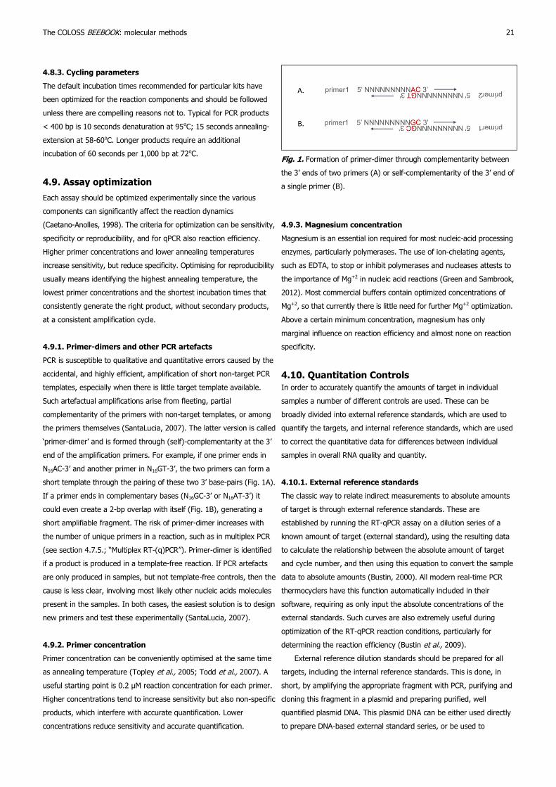
Fig. 1. Formation of primer-dimer through complementarity between

the 3’ ends of two primers (A) or self-complementarity of the 3’ end of

a single primer (B).

4.8.3. Cycling parameters

The default incubation times recommended for particular kits have

been optimized for the reaction components and should be followed

unless there are compelling reasons not to. Typical for PCR products

< 400 bp is 10 seconds denaturation at 95oC; 15 seconds annealing-

extension at 58-60oC. Longer products require an additional

incubation of 60 seconds per 1,000 bp at 72oC.

4.9. Assay optimization

Each assay should be optimized experimentally since the various

components can significantly affect the reaction dynamics

(Caetano-Anolles, 1998). The criteria for optimization can be sensitivity,

specificity or reproducibility, and for qPCR also reaction efficiency.

Higher primer concentrations and lower annealing temperatures

increase sensitivity, but reduce specificity. Optimising for reproducibility

usually means identifying the highest annealing temperature, the

lowest primer concentrations and the shortest incubation times that

consistently generate the right product, without secondary products,

at a consistent amplification cycle.

4.9.1. Primer-dimers and other PCR artefacts

PCR is susceptible to qualitative and quantitative errors caused by the

accidental, and highly efficient, amplification of short non-target PCR

templates, especially when there is little target template available.

Such artefactual amplifications arise from fleeting, partial

complementarity of the primers with non-target templates, or among

the primers themselves (SantaLucia, 2007). The latter version is called

‘primer-dimer’ and is formed through (self)-complementarity at the 3’

end of the amplification primers. For example, if one primer ends in

N16AC-3’ and another primer in N16GT-3’, the two primers can form a

short template through the pairing of these two 3’ base-pairs (Fig. 1A).

If a primer ends in complementary bases (N16GC-3’ or N16AT-3’) it

could even create a 2-bp overlap with itself (Fig. 1B), generating a

short amplifiable fragment. The risk of primer-dimer increases with

the number of unique primers in a reaction, such as in multiplex PCR

(see section 4.7.5.; “Multiplex RT-(q)PCR”). Primer-dimer is identified

if a product is produced in a template-free reaction. If PCR artefacts

are only produced in samples, but not template-free controls, then the

cause is less clear, involving most likely other nucleic acids molecules

present in the samples. In both cases, the easiest solution is to design

new primers and test these experimentally (SantaLucia, 2007).

4.9.2. Primer concentration

Primer concentration can be conveniently optimised at the same time

as annealing temperature (Topley et al., 2005; Todd et al., 2007). A

useful starting point is 0.2 µM reaction concentration for each primer.

Higher concentrations tend to increase sensitivity but also non-specific

products, which interfere with accurate quantification. Lower

concentrations reduce sensitivity and accurate quantification.

The COLOSS BEEBOOK: molecular methods 21

4.9.3. Magnesium concentration

Magnesium is an essential ion required for most nucleic-acid processing

enzymes, particularly polymerases. The use of ion-chelating agents,

such as EDTA, to stop or inhibit polymerases and nucleases attests to

the importance of Mg+2 in nucleic acid reactions (Green and Sambrook,

2012). Most commercial buffers contain optimized concentrations of

Mg+2, so that currently there is little need for further Mg+2 optimization.

Above a certain minimum concentration, magnesium has only

marginal influence on reaction efficiency and almost none on reaction

specificity.

4.10. Quantitation Controls

In order to accurately quantify the amounts of target in individual

samples a number of different controls are used. These can be

broadly divided into external reference standards, which are used to

quantify the targets, and internal reference standards, which are used

to correct the quantitative data for differences between individual

samples in overall RNA quality and quantity.

4.10.1. External reference standards

The classic way to relate indirect measurements to absolute amounts

of target is through external reference standards. These are

established by running the RT-qPCR assay on a dilution series of a

known amount of target (external standard), using the resulting data

to calculate the relationship between the absolute amount of target

and cycle number, and then using this equation to convert the sample

data to absolute amounts (Bustin, 2000). All modern real-time PCR

thermocyclers have this function automatically included in their

software, requiring as only input the absolute concentrations of the

external standards. Such curves are also extremely useful during

optimization of the RT-qPCR reaction conditions, particularly for

determining the reaction efficiency (Bustin et al., 2009).

External reference dilution standards should be prepared for all

targets, including the internal reference standards. This is done, in

short, by amplifying the appropriate fragment with PCR, purifying and

cloning this fragment in a plasmid and preparing purified, well

quantified plasmid DNA. This plasmid DNA can be either used directly

to prepare DNA-based external standard series, or be used to

synthesize RNA transcripts which in turn are quantified accurately and

used to prepare RNA-based external standard series. DNA-based

standards tend to be more sensitive and reproducible but RNA-based

standards are more realistic and also take the cDNA reaction

efficiency into account. The professional literature is divided on the

issue, with good arguments for both approaches (Pfaffl and Hageleit,

2001). Both curves still require several positive control RNA samples

per run, to normalize between runs for differences in reagent mixtures

and, in the case of the DNA curve, to account for the reverse

transcription step as well.

Reference standards from PCR products:

1. Amplify the target fragment by RT-PCR.

2. Confirm the amplification and absence of secondary products

with electrophoresis.

3. If there are secondary products, excise the correct fragment

under low-intensity UV light.

4. Purify the fragment using a commercial DNA affinity

purification column.

The purified PCR fragments can be used directly to prepare an

external reference standard, as follows:

1. Estimate the DNA concentration of the fragment in ng/µl,

using spectrophotometry (e.g. Nanodrop, section 3.2.1) or

fluorimetry (e.g. Qubit®; www.inVitrogen.com).

2. Estimate the molecular weight of your fragment.

This can be done exactly, based either on actual sequence or on

fragment length, in the tools tab at www.currentprotocols.com. An

approximate estimate for fragments within the 100-1000 bp range is:

MWdsDNA = bp x 617 ng/nmol

3. Convert the DNA concentration to copies/µl as follows:

copies/µl = [ng/µl]/[MWdsDNA] x [6.0221415 x 1014 copies/nmol]

4. Store the undiluted DNA fragment in aliquots at -80oC.

5. Prepare a working quantification standards series by serial ten

-fold dilution of the DNA fragment, ranging from 1012 – 100

copies/µl, in 10 ng/µl yeast or E. coli tRNA (Bustin et al., 2009),

to minimize loss of standard DNA due to adsorption to the

microcentrifuge tube walls.

Whether or not the PCR products are used directly for preparing

external reference standards, they should also be cloned: for confirmation

of the fragment by sequencing, for long-term preservation of a

positive DNA control and for the synthesis of RNA-based external

reference standards. The fragment should be cloned into a T/A plasmid

cloning vector that has T7 and T3 RNA promoters either side of the

cloning site. Many molecular supply companies market such T/A cloning

vectors, which are specially prepared for cloning PCR fragments.

22 Evans et al.

1. Clone PCR fragments.

Protocols for cloning PCR fragments are beyond the scope of this

paper. For this, the reader is referred to the product manuals

provided by commercial suppliers of T/A cloning kits, and specialist

manuals, such as the outstanding and long-established “Molecular

cloning: a laboratory manual“, by Green and Sambrook (2012).

2. Confirm candidate bacterial clones by colony PCR. This is a

conventional 20 µl PCR reaction using the primers and

amplification profile appropriate for the target, containing a

small smudge of primary bacterial colony as template.

3. Run the colony-PCR products on an agarose gel (Green and

Sambrook, 2012, see section 3.2.1).

4. Identify those colonies containing a plasmid with a cloned

target.

5. Prepare small-scale liquid cultures of positive bacterial clones

(Green and Sambrook, 2012).

6. Mix 0.5 ml of liquid bacterial culture with 0.5 ml 50% sterile

glycerol and store this at -20oC (glycerol stocks).

7. Prepare plasmid DNA from the remaining liquid bacterial

culture, using either a commercial plasmid purification kit or

home-made reagents recommended in a molecular laboratory

manual (Green and Sambrook, 2012).

Make sure that the protocol includes an RNAse step, to digest any

bacterial RNA.

8. Purify the plasmid DNA on a commercial DNA affinity

purification column.

9. Sequence the plasmid, using universal plasmid-based primers.

This is best done at specialist commercial facilities.

10. Confirm the presence of the insert in the plasmid from the

sequence data, and the orientation of the insert in the

plasmid.

11. Estimate the DNA concentration of the plasmid in ng/µl, using

spectrophotometry (e.g. Nanodrop, section 3.2.1) or

fluorimetry (e.g. Qubit®; www.InVitrogen.com). dsDNA

A260 1,0 = 50 ng/µl

12. Estimate the molecular weight of the plasmid + insert, by

combining their lengths in bp and converting either exactly at

www.currentprotocols.com or approximately as follows:

MWdsDNA = (bpplasmid + bpinsert) x 607.4 + 157.9 ng/nmol

13. Convert the DNA concentration to copies/ul as follows:

copies/µl = [ng/µl]/[MWdsDNA] x [6.0221415 x 1014 copies/nmol]

14. Store the undiluted plasmid in aliquots at -80oC.

15. Prepare a working quantification standards series by serial ten

-fold dilution of the plasmid, ranging from 1012 – 100 copies/µl,

in 10 ng/µl yeast or E. coli tRNA (Bustin et al., 2009).

RNA-based external reference standards

1. Transcribe RNA from purified plasmid DNA, using either the T7

or the T3 promoter, depending on the orientation of the insert

and the desired strand polarity of the RNA.

2. Linearize the plasmid with a restriction enzyme that digests

right after the cloned fragment, in the desired orientation.

This ensures that the RNA transcripts have a defined length.

3. Transcribe the digested plasmid with a specific commercial T3/

T7 RNA transcription kit.

Follow the corresponding instructions. Alternatively, detailed protocols

with home-made reagents can be found in Green and Sambrook

(2012).

4. Digest the synthetic, transcribed RNA with DNAse, as

recommended by the kit manufacturer.

This is to remove contaminating plasmid DNA which may co-amplify

and thus interfere with correct quantification.

5. Purify the DNAse-treated RNA on RNA affinity purification

columns.

6. Estimate the RNA concentration in ng/µl, using

spectrophotometry (e.g. Nanodrop, section 3.2.1) or fluorimetry

(e.g. Qubit®; InVitrogen). ssRNA A260 1,0 = 40 ng/µl

7. Calculate the insert size (number of bases from the T3/T7

promoter site to the restriction enzyme site on the other side

of the insert used for digesting the plasmid).

8. Estimate the molecular weight of the RNA transcript either

exactly at www.currentprotocols.com or approximately as

follows:

MWssRNA = nt x 320.5 + 159.0 ng/nmol

9. Convert the concentration of the synthetic RNA to copies/µl as

follows:

copies/µl = [ng/µl]/[MWssRNA] x [6.0221415 x 1014 copies/

nmol]

10. Store the undiluted RNA in aliquots at -80oC.

11. Prepare a working quantification standards series by serial ten

-fold dilution of the RNA, ranging from 1012 – 100 copies/µl.

Do not use an RNA carrier for preparing the dilution series, since

this carrier RNA will participate in the reverse transcriptase reaction

and thereby significantly affect quantification!! Instead, dilute either in

nuclease-free water or in 10 ng/µl of a neutral DNA carrier, obtained

from a commercial source.

4.10.2. Internal reference standards

Unfortunately, external standards cannot correct for factors unique to

each sample that affect the RT and/or PCR reactions, such as RNA

quality and quantity, enzyme inhibitors, sample degradation, internal

fluorescence etc. To correct for these factors, internal reference

standards are used. These come in two forms:

The COLOSS BEEBOOK: molecular methods 23

4.10.2.1. Exogenous internal reference standards

Exogenously added internal reference standards are a pure, unrelated

RNA of known concentration and integrity that is added to each

sample prior to analysis. Such RNAs can be bought commercially (for

example, Ambion’s RNA250) and can be used to correct the data for

the presence of enzyme inhibitors in individual RNA samples

(Tentcheva et al., 2006). The amount added per reaction should be

low; < 1% of the amount of sample RNA, so as not to affect the

RT-qPCR reaction efficiencies.

4.10.2.2. Internal reference standards

Endogenous internal reference standards (commonly called

‘housekeeping genes’) are relatively invariant host mRNA targets

present in every sample that can be used to normalize quantitative

data for minor variations between samples in RNA quality and quantity

(Bustin et al., 2009; Radonić et al., 2004). The problem is that it is

impossible to prove categorically that the expression of any candidate

‘invariant’ gene is not affected by the expression of the target gene

(Radonić et al., 2004). For this reason it is currently recommended to

use a battery of 3 or 4 internal controls, from different classes of

genes (metabolic enzymes, structural proteins, transcription factors,

ribosomal proteins etc.) and construct a control-gene index, with

which to normalise between samples (Bustin, 2000). Common internal

reference standards for honey bee research are β-actin (Chen et al.,

2005a; Shen et al., 2005a; 2005b; Locke et al., 2012), rRNA

(Chantawannakul et al., 2006), microsomal glutathione-S transferase

(Evans and Wheeler, 2000; Gregory et al., 2005); ribosomal proteins

RP-S5 (Evans, 2004; 2006; Wheeler et al., 2006), RP49 (Corona et al.,

2005; Yañez et al., 2012), RP-S8 (Kucharski and Maleszka, 2002), and

transcription factors eIF3-S8 (Grozinger et al., 2003) and eF1α (Toma

et al., 2000; Yamazaki et al., 2006).

One technical difficulty with endogenous internal reference

standards is the presence of contaminating genomic DNA in a sample,

which could be amplified instead of the mRNA. There are two

solutions to this:

Digest the RNA sample with DNAse prior to RT-PCR.

Many RNA purification kits come with this option.

Design the RT-PCR assay such that the primers are separated

by a (large) intron in the genomic copy of the gene.

Only the spliced mRNA will be amplified by the assay (Bustin, 2000).

Such intron-spanning primers have been designed for the honey bee

RP49 mRNA and B-actin-isoform-2 mRNA (de Miranda and Fries, 2008;

Yañez et al., 2012; Locke et al., 2012).

As stated above, all internal reference standards also require their

own external standards for accurate quantification. The inclusion of

internal reference standards obviously greatly increases the cost of a

project. The inclusion of internal controls is therefore one of several

parameters to be decided on when starting a project, based on the

projects’ objectives, requirement for quantitative precision and

available finances. Generally, the need for internal controls is greater

for fully quantitative experiments with highly detailed analysis of

relatively few samples. The need is much less for semi-quantitative

survey-type studies, with fewer specific analyses and large numbers

of samples.

4.10.2.3. External standard for viral target quantification

1. Extract RNA (Qiagen RNeasy® Mini Kit and QiaShredder®,

according to manufacturer´s protocol) of bees with an RNA

target (in this example DWV).

2. Generate an external standard by amplifying a DWV genomic

fragment of 1520 bp via RT-PCR, using the primers Fstd

(5´-GGACCATCCTTCCAGTCTACGAT-3´) and Bstd

(5´-CTGTAGGTTGTGCTCCTGATGAAGA-3´) and the one-step

RT-PCR kit from Qiagen.

3. This fragment contains the 354 bp fragment, which can be

amplified by the primer pair F1/B1 (Genersch, 2005), for

quantification.

4. Quantify the number of PCR-fragments via photometric

analysis at 260 nm wavelength (Nanodrop, section 3.2.1).

5. Prepare a dilution series from the initial concentration through

three orders (10-fold dilutions) of concentrated solutions.

This set of fixed dilutions will be used to ensure that PCR

efficiency is maintained and to identify the precise predicted copy

number for a particular Cq threshold.

4.11. Microarrays

A microarray is a powerful multiplex detection technology consisting

of an ordered array of hundreds of molecular probes specific for

different target RNAs bound to a solid support, usually a slide. The

target sequences in an RNA sample are hybridized to these probes

and these hybridization events are detected by a variety of, usually

optical, detection chemistries (de Miranda, 2008). The power of the

technology lies in the massive multiplexing potential where the

relative and absolute amounts of hundreds of different targets can be

determined simultaneously (Cheadle et al., 2003; Gentry et al., 2006).

As molecular biology, pathology and diagnostics moves away from

single organism/gene effects to surveying interactions among pathogens

and (host) genes, microarray-based diagnostics will become increasingly

relevant. Microarray printing technology is becoming cheaper and

more reliable, and single-use disposable microarrays for specific multi-

target diagnosis are increasingly available (Yuen et al., 2003;

Lieberfarb et al., 2003; Noerholm et al., 2004; Lin et al., 2004;

Perreten et al., 2005; Fiorini et al., 2005). Uniformity of hybridisation

across the microarray, important for reliability in quantitation, is

maximized with a range of nano-technological innovations (Yuen et al.,

2003; Noerholm et al., 2004; Fiorini and Chiu, 2005), improved

24 Evans et al.

oligonucleotide design (Rouillard et al., 2003) and with replication of

the spots or even whole arrays (an array of arrays) across the slide.

The probe-target hybridisation can be detected through FRET-based

probes, SYBR-green-I dye, or labelling of the nucleic acid sample

containing the target sequences. Microarray technology can also be

combined with quantitative RT-PCR, multiplex (pyro)sequencing and

label-free electronic or optical detection technologies to increase the

speed, accuracy, specificity or information content of the diagnosis

(Weidenhammer et al., 2002; Erali et al., 2003; Gharizadeh et al.,

2003; Fixe et al., 2004).

Numerous honey bee arrays have already been designed for

different research purposes (Whitfield et al., 2002; Evans and

Wheeler, 2000; 2001; Robinson et al., 2006). A microarray has also

been developed for the semi-quantitative detection of honey bee

viruses (Table 5 in Glover et al., 2011) which will be developed further

for diagnostic purposes.

Microarrays can also be developed for serology-based detection of

proteins (Sage, 2004), using a similar approach as the sandwich

ELISA (Enzyme-Linked ImmunoSorbent Assay: see de Miranda et al.,

2013). The probe-target recognition events are visualized and

detected using similar detection chemistries as for nucleic acid-based

microarrays.

4.12. Northern blots using DIG labelling

The primary advantage of using Northern blot analyses for identifying

specific predicted RNA’s, versus a PCR-based method, comes in the

ability to predict the size of the entire transcript that is targeted using

standard gel size markers. This is key especially when transcripts are

subjected to editing (splice variants or enzymatic cutting as for small

RNAs) and editing must be validated using a technique other than

PCR. In addition, since probe binding is more permissive of nucleotide

changes, Northern blots can be used to verify transcripts that might

have mutations at primer sites used for PCR. In addition, this

approach has somewhat lower vulnerability to point mutations that

might cause a specific primer pair to fail to amplify a predicted target.

The disadvantage to using Northern blots versus a PCR method as

above is in time and expense and in a somewhat reduced ability to

quantify transcript abundance. The below protocol avoids the use of

radio-isotopic nucleotides as probes.

4.12.1. Agarose /formaldehyde gel electrophoresis

What follows is a standard protocol for denaturing gels suitable for

linear separation of RNA strands:

1. Be RNase free!! Use gel apparatus designated for RNA. Wipe

apparatus with “RNaseAway” and rinse thoroughly with RNAse

-free water.

2. Prepare 100 ml of 1% agarose/formaldehyde gel:

1. Dissolve 1 g agarose in 72 ml DEPC-treated water in a 250 ml

glass flask.

2. Cool to 60oC in a water bath.

3. Add 10 ml of 5X MOPS running buffer (200 mM MOPS

buffer, 50 mM Sodium acetate, 20 mM EDTA, pH 7.0) and

18 ml of 37% formaldehyde.

Precautions: Formaldehyde vapours are toxic. Prepare the

gel in a fume hood.

3. Pour the gel to the gel tank and allow it to set.

4. Add sufficient 1X MOP running buffer to fill the tank in order

to cover the gel and remove the comb carefully.

5. To prepare samples for gel electrophoresis, mix:

11 µl of each RNA sample (0.5-1 µg/µl),

5 µl 5X MOPS running buffer,

9 µl 37% formaldehyde,

25 µl of 50% formamide.

6. Heat the sample at 65oC for 15 min.

7. Cool on ice for 2 min.

8. Add 3 µl loading dye mix and 2 µl ethidium bromide (0.5 mg/ml).

9. Run the gel immediately after loading samples.

10. When the gel dye bands have separated and migrated at least

2-3 cm into the gel, or as far as 2/3 the length of the gel,

visualize under UV light and take picture.

The 28s and 18sribosomal RNA (rRNA) should appear as sharp

bands on the gel with no apparent smearing from degradation. The

28S rRNA band should be approximately twice as intense as the 18S.

4.12.2. Assembly of the transfer setup and transfer of RNA

from gel to membrane

1. To prepare a gel for transfer, rinse the gel in DEPC-treated

water twice for 20 min to remove the formaldehyde, which

will otherwise interfere with transfer of RNA from gel to the

membrane.

2. Soak the gel in RNase-free 20X SSC (3.0 M NaCl and 0.3 M

sodium citrate, pH 7.0) for 45 min before proceed to setting

up the transfer.

3. Cut uncharged nitrocellulose membrane to size of gel.

4. Soak the membrane in water for 2-3 min to wet .

5. Float in 20X SSC.

The transfer is conducted by the capillary method (Fig. 2).

1. Place a piece of thick blotting paper on the top of a glass plate

that is elevated by four rubber stoppers placed near each

corner of a baking glass dish.

2. Drape the ends of the wick blotting paper over the edges of

the plate.

3. Fill the glass dish with RNase-free 20X SSC until the wick

blotting paper on the top of glass plate is completely wet.

4. Squeeze out all air bubbles by rolling with a glass rod or

pipette.

The COLOSS BEEBOOK: molecular methods 25

5. Place the gel facing down on the wet blotting paper.

6. Squeeze out air bubbles by rolling a glass pipette.

7. Cut a small triangular piece from the top left-hand corner to

simplify orientation.

8. Place the wetted membrane on the surface of the gel by

aligning the cut corners.

9. Get rid of any air bubbles under the membrane by rolling a

glass pipette.

10. Cut 4-5 sheets of Whatman 3MM paper to the same size as

membrane.

11. Place on top of the membrane.

12. Place a stack of paper towels on top of the Whatman 3MM

papers.

13. Add a 200-500 g weight to hold everything in place.

14. Allow the transfer of RNA to proceed by capillary action

overnight.

15. Disassemble the transfer stack at the next day.

16. Rinse the membrane briefly in 6X SSC.

17. Immobilize RNA to the blot by UV cross linking while the

membrane is still damp.

4.12.3. Preparation of DIG labelling (non-radioactive) probe

While DNA probes can also be used to detect RNA targets, a DIG-

labeled RNA probe is ideal for detecting RNA on a Northern blot

because RNA probes (riboprobes) that are transcribed in vitro are able

to withstand more rigorous washing steps preventing some of the

background noise. RNA probes give better sensitivity for detecting low

amounts of RNA target than DNA probes. The following protocol is

based on the Roche DIG RNA Labelling Kit, SP6/T7.

Fig. 2. Schematic diagram of the process used to transfer nucleic

acids from a gel onto a binding membrane.

1. Linearize the recombinant plasmid DNAs with the target insert

by cutting a restriction enzyme cleavage site downstream

from the cloned insert using a restriction enzyme that creates

5’ overhangs (the choice of this enzyme will depend on the

sequence of both the plasmid and insert).

2. After restriction digestion, purify the DNA by spin column

purification or via phenol/chloroform/isoamyl alcohol

extraction and ethanol.

This is commonly referred to as the ‘plasmid mini-prep’ and there

are numerous commercial and home-made recipes for doing so that

all work well.

3. Add the 2 μg purified template DNA to the following

transcription reaction mixture to make 26 µl probe as follows:

4 µl 10X NTP labelling mixture,

4 µl 10X Transcription buffer,

2 µl Protector RNase Inhibitor,

4 µl RNA Polymerase SP6/or T7.

Adjust the volume with additional water until a final volume of 26 µl.

4. Place transcription reaction in the 37°C incubator for 2 hours.

Longer incubations do not increase the yield of labeled RNA.

5. Stop reaction with 2μl 0.2M EDTA (pH 8.0).

Labeled probes are stable for at least one year at -15 to -25°C.

4.12.4. Hybridization analysis

(Roche Applied Science DIG Easy® Hyb, DIG Wash and Block Buffer

Set, CSPD®Ready-to-use protocol)

1. Pre-hybridize the blot with pre-warmed DIG Easy® Hyb

(10– 15 ml per 100 cm2) in a specialized hybridization bag or

any sealable container:

1. Incubate the blot for 30 min at 65°C.

2. Agitate gently during the pre-hybridization step.

2. Pipette the desired volume of probe (50-100 ng probe per ml

hybridization buffer) into the hybridization bag.

3. Continue to incubate with rotation at 65°C for 10-16 hours.

4. After the hybridization is complete, wash the blot in a tray

containing Low Stringency Buffer (2x SSC containing 0.1%

SDS) twice by incubating the tray at RT for 5 min with gentle

agitation.

5. Transfer the blot to preheated High Stringency Buffer (0.1x

SSC containing 0.1% SDS).

6. Incubate the blot twice (2 x 15 min, with shaking) in High

Stringency Buffer at 65°C.

7. After last wash, pull out the blot out of the hybridization

container.

8. Place it between two Whatman paper sheets.

Do not allow the membrane get too dry so the membrane can be

stripped and reused for hybridization.

9. Place blot onto a piece of Plastic wrap that is at least twice

the size of the membrane.

26 Evans et al.

10. Add 1 ml detection reagent (anti-digoxigenin-AP conjugate

and the premixed stock solution of CSPD® ready-to-use) to

stain the membrane and leave for 5 min.

11. Completely wrap up the blot with the plastic wrap.

12. Put it in a film cassette for chemiluminescent detection of

hybridization signals.

4.13. In situ hybridization

4.13.1. Tissue fixation

1. Dissect out individual tissues.

2. Wash tissues with cold PBS 2-3 times.

3. Fix tissues in freshly made 4% paraformaldehyde in 100mM

PBS (pH 7.0) overnight at 4oC.

4. Rinse in nuclease-free water three times.

5. Store tissues in 70% ethanol at 4oC until further use.

6. For tissue dehydration, carry out successive incubation in

ethanol (70%, 95% and 100%) and xylol (2 x 5 min each).

7. Embed in paraffin.

8. Cut Paraffin sections into 2-5 micron thick segments.

9. Mount on poly-L-lysinated slides which are to be stored at 4°C

overnight.

10. To rehydrate the sections prior to hybridization:

1. Carry out descending concentration of ethanol (100%,

95% and 70%).

2. Dewax in xylol.

3. Treat with proteinase K (10 ug/ml) for 30 min.

4. Acetylate with 0.33% (v/v) acetic anhydride in 0.1 M

triethanolamine-HCl (pH 8.0) for 10 min.

4.13.2. Preparation of DIG labelling (non-radioactive) probe

Using Roche DIG RNA Labelling Kit, SP6/T7. The same procedures as

for Northern blot (see section 4.12.).

4.13.3. Hybridization Analysis

1. Pre-hybridize the sections in pre-hybridization solution (50%

formamide, 5X SSC, 40 µg/ml salmon sperm) at 58oC for two

hours.

2. Incubate in hybridization buffer with Dig-labeled TARGET

probe solution to a concentration of 100-200 ng/ml of probe

in pre-hybridization solution at 58oC overnight.

3. After hybridization, wash the sections twice in low stringency

wash solution (2X SSC, 0.1% SDS) at room temperature for

five minutes.

4. Wash twice in high stringency wash solution (0.1 × SSC, 0.1%

SDS) at 52oC for 15 min.

Note: The hybridization signals are detected with Alkaline

phosphatase (AP)-labeled sheep anti-DIG antibody conjugate (Roche

Applied Science).

5. Add the conjugate solution to the dry sections.

6. Incubate at 4°C for two hours in a chamber in which humidity

is maintained at > 70% relative humidity.

7. Rinse the slides three times with washing buffers.

8. Perform the colour development by adding the buffer solution

containing nitroblue tetrazolium (NBT) and 5-bromo-4-chloro-

3-indoyl phosphate (BCIP) on the tissue sections.

9. Incubate for three to six hours at RT protected from bright

light.

10. Stop the colour reaction by a 5 min wash in Tris/EDTA (0.1

mM, pH 8.0).

11. Remove the non-specific staining in 95% EtOH overnight.

12. Rehydrate the sections through:

1. Successive incubation in ethanol (70%, 95%, and 100%).

2. Incubation in xylol (2 X15 min each).

13. Mount in Eukitt® resin (Sigma).

Note: Negative control reactions include regular dUTP instead of

DIG-labeled TARGET probe.

14. Observe and photograph In Situ hybridization slides under a

light microscope.

The hybridization signals are shown by dark blue sites where the

DIG-labeled probe bound directly to the viral RNA. The section of

negative control will stain pink only with the nuclear fast red.

5. Proteomic methods

5.1. Introduction

Proteins are the ultimate functional product of most gene expression

so optimally one would prefer to look at proteins when trying to

understand the mechanisms an organism uses to respond to a given

condition. As with any other biomolecule, tools for identifying and

quantifying proteins are a prerequisite to their successful study. Single

proteins are typically detected using antibodies but very few

antibodies have been generated against bee proteins and none have

been commercialized. Of all the analytical methods available for

studying proteins, mass spectrometry is the most sensitive, most

accurate and least biased. Proteins can be identified by mass

spectrometry by first hydrolyzing them with a specific protease such

as trypsin. The masses and fragmentation patterns of the resulting

peptides can then be determined and used to identify the peptides

individually and the protein(s) they came from (i.e. proteomics). This

process works best when all possible proteins that might be present

are known and is only really successful when an organism’s genome

has been sequenced. To this end, in recent years proteomics has

begun to be applied in bees towards understanding a range of

paradigms.

Where is the future of proteomics research in bees heading?

Mapping protein expression across all tissues and castes in adult bees

is the logical next step after sequencing the bee genome. The

The COLOSS BEEBOOK: molecular methods 27

genome helps to determine which proteins may be present but where

are those proteins expressed? The protein expression atlas in bees

will tell that and will mark a significant step forward for bees as a

model system as this would be the first such comprehensive atlas in

any multicellular organism. Additional protein-based methods (protein

extraction and immunochemical assays for protein abundance) are

covered in further detail in the BEEBOOK paper on physiology and

biochemistry (Hartfelder et al., 2013).

6. Population genetics

6.1. Introduction

Measuring the current variation in genetic traits within and across

populations can give insights into past movement of individuals,

population size, and the association of specific genetic histories with

honey bee biological traits such as behaviour, disease resistance, and

colony life histories. Honey bees, thanks to human transport and

breeding, are made up of numerous and often entwined genetic

lineages and one aim of population-genetic analyses are to resolve

these connections.

6.2. Mitochondrial DNA analysis

In principle, one honey bee (worker or drone) per colony is enough to

determine the maternal origin of the whole colony given the maternal

inheritance of mitochondrial DNA (mtDNA), i.e. all the daughter

workers and son drones from one honey bee queen share the same

molecule. Due to the risk of drifting between colonies, it is ideal, and

in some cases essential, to make this one collected individual of a life

stage where host colony is unambiguous (e.g., a developing bee or

one observed exiting from a brood cell). In cases where this is not

possible, pre-flight worker bees could be substituted, although it is

arguably worth sampling more than one individual to avoid mistakes

in assigning colony heritage.

The most widely used mitochondrial region for population genetic

studies is the intergenic region located between the tRNAleu and cox2

(subunit 2 of the cytochrome oxidase) genes. This region shows

length and sequence variation that allows discrimination of honey bee

evolutionary lineages (Garnery et al., 1993). It is composed of two

types of sequences: P and Q. The sequence P can be absent (lineage

C from east Europe) or present in four different forms: P (lineage M

from west Europe), P0 (lineages A from Africa and O from Near East),

P1 (Atlantic African sub-lineage) and P2 (restricted to the Y lineage

from Ethiopia; De la Rúa et al., 2009). The number of Q sequences

and the sequence variation developed through a RFLP test with the

restriction enzyme DraI (Garnery et al., 1993) can be used to

determine the haplotype within each lineage. Below is the protocol to

determine the mitochondrial haplotype, modified from Garnery et al.

(1993) by including a new thermal regime for PCR and optimizing the

chemistry of PCR reactions. A full description of how this locus can

discriminate among honey bee ecotypes is presented in the BEEBOOK

paper on characterizing subspecies and ecotypes by Meixner et al.

(2013).

1. Honey bee samples are immediately transferred into tubes

with absolute EtOH and preserved at -20°C until DNA

extraction. A single or two legs from one individual are

enough to extract total DNA following the Chelex®-based

(Biorad, Inc.) protocol (Walsh et al., 1991; see section 3.2.3.).

2. PCR amplify the intergenic region with the primers E2

(5’-GGCAGAATAAGTGACATTG-3’) located at the 5’ end of the

gene tRNAleu and H2 (5’-CAATATCATTGATGAACC-3’) located

close to the 5’ end of the gene cox2 (Garnery et al., 1993).

This amplification can be performed by using Ready-To-Go TM PCR

Beads (product code 27-9557-01, GE Healthcare), that are pre-mixed

and pre-dispensed reactions for PCR featuring, therefore reducing the

pipetting steps and the chances to handling error. They contain all the

necessary reagents for a 25 µl reaction volume.

3. Add 20.2 µl of PCR-quality water to each tube.

4. Mix by gently flicking it with the fingers.

5. Add 0.4 µl of each primer (10 mM) and vortex and centrifuge

the mix to get all the components at the bottom of the tubes.

6. Add 4 µl of DNA extraction solution and mix.

7. Place the reaction mixtures in a thermo cycler with the

following amplification program:

Denaturation at 94 °C for 5 min,

Followed by 35 cycles of:

94 °C for 45 sec,

48 °C for 45 sec,

62 °C for 2 min,

Final elongation step of 20 min at 65 °C.

8. To identify successful amplicons, 2 µl of the PCR product of

each sample are electrophoresed in a 1.5% agarose gel (see

section 3.2.1) with ethidium bromide included and

photographed over a UV light screen.

9. Aliquots of the PCR product are then digested with the

endonuclease DraI (recognition site 5’-TTTAAA-3’) by adding:

10X endonuclease buffer to a final concentration of 1X,

0.06U of DraI/,

10 µL of PCR product,

Incubate at 37°C overnight.

10. To determine RFLP patterns, the digested products of each

sample are electrophoresed in a 4% agarose Nusieve® or

Metaphor® (Lonza Biosciences) gel at 100 volts for ca. 1 hour

30 min and photographed over a UV light screen.

11. At least one sample with a characteristic RFLP pattern should

be directly sequenced using the same primers as for the

amplification.

28 Evans et al.

12. Prior to sequencing, purify PCR products:

Either with QIAquick® PCR Purification Kit (Qiagen).

Alternatively, PCR products can be purified with isopropanol

and 5 M ammonium acetate as follows:

1. To 10 µl of PCR product add:

7 µl of 5 M ammonium acetate,

17 µl of isopropanol.

2. Leave 10 min at room temperature.

3. Centrifuge 30 min to 13,500 rpm.

4. Discard the supernatant.

5. Add 500 µl of cold 70% EtOH.

6. Centrifuge 5 min at 13,500 rpm.

7. Remove supernatant and allow to dry overnight.

8. Re-suspend in 30 µl of water.

6.3. Nuclear DNA analysis

Nuclear markers are biparentally inherited and allow genotyping of

workers to obtain information from both the mother queen and the

drones she has mated with. Nuclear analyses of A. mellifera involve

widely used microsatellites and more recently, single nuclear

polymorphisms or SNPs.

6.3.1. Microsatellites

Microsatellites consist of short motifs (one to six nucleotides) that are

repeated from four to 20+ times at points scattered across all

eukaryotic genomes. They are useful as markers for genetic structure

since the number of repeats at any given locus is unstable and new

repeat variants are constantly arising by mutation and being lost by

drift and other population-level events. Strategies to screen a total of

550 polymorphic microsatellite loci have been described in A. mellifera

(Solignac et al., 2003), and many thousands more are found in the

complete honey bee genome (Honey Bee Genome Sequencing

Consortium, 2006). The protocol described here has been used to

analyse the temporal genetic variation of island honey bee

populations (Muñoz et al., 2012), the mating frequency of the Iberian

honey bee (Hernández-García et al., 2009) and the population genetic

structure of European honey bees (Muñoz et al., 2009; see also the

BEEBOOK paper on characterizing subspecies and ecotypes by

Meixner et al. (2013) for a full review of the use of microsatellites in

determining honey bee ecotypes). It takes advantage of multiplexing,

whereby multiple loci are screened in a single PCR reaction and size

assay. These loci are widely used, and it is subsequently possible to

compare allelic counts and genotypes across different studies.

6.3.1.1 Microsatellite reaction mix

To prepare the reaction mix, add:

1X reaction buffer (provided as a 10x solution with Taq

polymerase),

1.2 mM MgCl2,

0.3 mM of each dNTPs,

0.4 µM of each primer,

1.5 U Taq polymerase,

> 5 ng DNA (provided in 2µl DNA solution).

6.3.1.2 Primers for multiplexed honey bee microsatellite loci

A113-F-(FAM) CTC GAA TCG TGG CGT CC

A113-R CCT GTA TTT TGC AAC CTC GC

A007-F-(NED) GTT AGT GCC CTC CTC TTG C

A007-R CCC TTC CTC TTT CAT CTT CC

AP043-F-(VIC) GGC GTG CAC AGC TTA TTC C

AP043-R CGA AGG TGG TTT CAG GCC

AP055-F-(PET) GAT CAC TTC GTT TCA ACC GT

AP055-R CAT TCG GTA TGG TAC GAC CT

B124-F-(FAM) GCA ACA GGT CGG GTT AGA G

B124-R CAG GAT AGG GTA GGT AAG CAG

6.3.1.3 Thermal cycling conditions for multiplex PCR

Incubate the samples as follows:

5 min at 95°C,

Followed by 30 cycles:

95°C for 30 sec,

54°C for 30 sec,

72°C for 30 sec,

Final extension is 30 min at 72°C.

6.3.1.4 Size estimation of PCR products

PCR products are visualized by capillary electrophoresis and sized with

an internal size-standard (e.g., using the Applied Biosystems or

MegaBACE systems, both of which have extensive use for

microsatellite scoring). Alleles are subsequently scored using

GeneMapper v3.7 software (Applied Biosystems™). It is also possible

to measure microsatellite size variants using large denaturing

polyacrylamide gels (e.g. Evans, 1993) although this method has

fallen from favour do to the hazards of polyacrylamide and difficulties

in manually scoring allele sizes.

Once genotypes of samples have been established, microsatellite

data are well suited for assessing parentage of nestmates (Evans,

1993), for standard population-genetic statistics including ecotype

determination (Estoup et al., 1993; reviewed by Meixner et al., 2013),

and for genome mapping (Solignac et al., 2003), among other uses.

6.3.2. Single-nucleotide polymorphisms (SNPs)

In the honey bee and other species for which extensive data have

been gathered on genomic sequence variants, it is possible to use

SNPs to reconstruct past migration events, and to separate races and

populations. A SNP is any validated nucleotide change between the

genomes of two or more samples, and SNP’s can occur both within

the coding regions (exons) of genes and in the vast regions that

The COLOSS BEEBOOK: molecular methods 29

separate genes or lie in non-coding parts of the genome. SNP

analyses are standard in human, veterinary, and agricultural systems,

and this approach will continue to increase as a viable option for the

study of honey bees. Unfortunately, high-throughput SNP genotyping

remains an expensive endeavour that requires cutting edge technologies

and the expertise often only available in a core laboratory facility or at

larger institutions. In addition, prior to genotyping the honey bee

sample of interest, a SNP assay must be developed (or purchased, if

commercially available) from sequence data relevant for the study

population. At present, there are only two SNP assays developed and

published for honey bees. The first one (Whitfield et al., 2006), which

consisted of 1536 SNP loci that were selected mainly based on spacing

criteria, was developed for genotyping using the Illumina GoldenGate™

assay and is not commercially available, although a honey bee SNP

database (over 1 million SNPs) is available at NCBI (http://

www.ncbi.nlm.nih.gov/snp/) and this resource could be exploited to

establish a system for genotyping. More recently, Spötter et al. (2011),

published a 44,000 SNP assay designed for analysis of varroa-specific

defence behaviour in honey bees. This assay uses Affymetrix™

technology, and it is now commercially available via AROS Applied

Biotechnology AS.

As illustrated in Spötter et al. (2011), development of a SNP assay

is a time and resource intensive undertaking, yet it can be designed to

address a specific objective (e.g., to investigate varroa-specific

defence behaviour). Once the design stage is accomplished, the assay

can then be used to genotype honey bee samples at hundreds to

thousands of loci via high-throughput technologies. Illumina®

technologies, for example, offer a number of options for high

throughput genotyping depending on the number of SNPs to be

interrogated. The GoldenGate assay, employed by Whitfield et al.

(2006), interrogates 96, or from 384 to 1,536 SNP loci simultaneously

(plex levels can be 384, 768, or 1,536). For genotyping a number of

SNPs larger than 6,000 up to 2,500,000 the Infinium assay (also a

product from Illumina) is required.

Both the GoldenGate assay and the Infinium assay take three

days for completion and require reasonable quality and accurately

quantified genomic DNA. DNA concentrations should be 50 ng/µl,

quantified a fluorometric assay (e.g., Picogreen) or spectrophotometry

(e.g., Nanodrop, section 3.2.1). DNA can be extracted from the

thoraces of honey bees that had been stored at -80°C or in absolute

EtOH. The GoldenGate assay involves several steps including DNA

activation for binding to paramagnetic particles, hybridization of

activated DNA with assay oligonucleotides, washing, extension,

ligation, PCR, hybridization onto the BeadChip, and finally analysis of

the fluorescence signal on BeadChip by the iScan System.

Unlike in the GoldenGate assay, where universal primers are used

to amplify SNP-reactive DNA fragments, in the Infinium assay

genomic targets hybridize directly to array-bound sequences.

Following hybridization onto the BeadChip, samples are extended and

fluorescently stained. As for the GoldenGate assay, the last step

consists of analysis of scanned BeadChips using the iScan System.

Genotype data generated by both assays using the iScan System (and

other systems), are then analysed using the GenomeStudio

Genotyping (GT) Module. The calls are automated but can be manually

verified and edited if necessary (e.g., if there are signs of unequal

proportions of an expected biallellic marker). Finally, summary

statistics and results are exported for further analyses using standard

population genetics software packages such as STRUCTURE (http://

pritch.bsd.uchicago.edu/structure.html).

With increasingly affordable sequencing costs allowed by next

generation technologies (e.g., 100 bp or shorter), it will be feasible to

carry out population-genetic and strain-identifying projects via whole-

genome sequencing. This technique involves a scan (usually 3-fold

sequencing depth or more, i.e., > 750 million sequenced bases for the

honey bee) of a genome or population of interest followed by an

alignment of those short reads to a reference genome (for the honey

bee this would be the genome assembly from HGSC, 2006). It is

relatively straightforward, using free programs available for download

(e.g., http://bioinformatics.igm.jhmi.edu/salzberg/Salzberg/

Software.html) to identify and in some cases quantify SNPs that differ

among samples. There are also public sites at which one can import

data and benefit from a maintained supercomputer dedicated to such

genomic analyses (e.g. https://main.g2.bx.psu.edu/). SNP analyses

derived from sequencing data have yet to make an impact on honey

bee science but they are expected to in the next few years.

7. Phylogenetic analysis of

sequence data

7.1. Introduction

The goal of this protocol is to provide the reader with an easy to use,

reliable, and technically appropriate method to choose, align and

analyse sequence data for phylogenetic analyses of taxa or genes of

interest. Analysis of highly conserved loci (i.e. rRNA, cytochrome

oxidase I) or population genetic studies from one species, require

nucleotide level data to achieve necessary resolution in tree topology.

Amino acid sequences are typically used when reconstructing

phylogenies from an encoded protein across a large evolutionary

distance, which can make alignment at the nucleotide level difficult.

Over time, one develops their preferred approach and programs to

use in this process, of which there are many. While the following

protocol reflects preferences of the authors, it is appropriate for a

wide variety of applications, user skill levels, and relies on freely

available programs with graphical user interface (GUI)-based options.

Detailed information on use is available from each of the program

sites, given below. As a disclaimer, concatenation of sequence data,

30 Evans et al.

while appropriate and employed for taxonomy classification, is a more

specific approach some users may wish to use but will not be

discussed here. Additionally, though PAUP is also widely used in

phylogenetic analyses, it requires a small fee and therefore is not

discussed here, though labs with frequent phylogenetic needs may

wish to purchase this program. MEGA and other software free to the

public can invoke many or all of the same phylogenetic analyses as

PAUP.

The steps to perform a phylogenetic analysis are:

1. Obtain and format sequences of interest.

2. Format sequence data in FASTA format.

3. Align sequence data.

4. Trim aligned sequence data to equal length.

5. Perform phylogenetic analyses.

Each step is described below in detail.

7.2. Obtaining and formatting sequences of

interest for phylogenetics

Once you have obtained DNA sequence data for your study, you may

wish to add accessioned sequence data to your analyses. This will be

particularly important if you want to root your phylogeny and provide

an outgroup (sequence(s) to which all of your sequences are distantly

related) to strengthen comparative interpretation of your data.

Accessions from nucleotide sequence data banks can be searched,

using a keyword(s) or via a BLAST search algorithm (i.e. blastn,

megablast, etc.), to identify homologues to your sequence of interest.

These include GenBank (via NCBI; (http://www.ncbi.nlm.nih.gov/),

EMBL-Bank (via EBI; http://www.ebi.ac.uk/embl/), and DNA Data

Bank of Japan (DDBJ; http://ddbj.sakura.ne.jp/). If using rRNA

sequence data, SILVA rRNA database (http://www.arb-silva.de/) can

be used to retrieve reference sequences that are quality-scored

(Pruesse et al., 2007).

7.3. Sequence data in FASTA format

For compatibility in downstream analyses, sequence data should be in

a single file and FASTA formatted. Sequence databases include

FASTA as an option for output format. An example of FASTA

formatted sequences retrieved from GenBank (abbreviated in length

for the sake of space):

>gi|21747902|gb|AY114459.1| Apis mellifera mellifera isolate

melli4 cytochrome oxidase subunit I (COI) gene, partial cds;

mitochondrial gene for mitochondrial product

CCCCGAATAAATAATGTTAGATTTTGATTACTTCCTCCCTCATTAT

TAATACTTTTATTAAGAAATTTATTTTACCCAAGACCAGGAACTG

GATGAACAGTATATCC

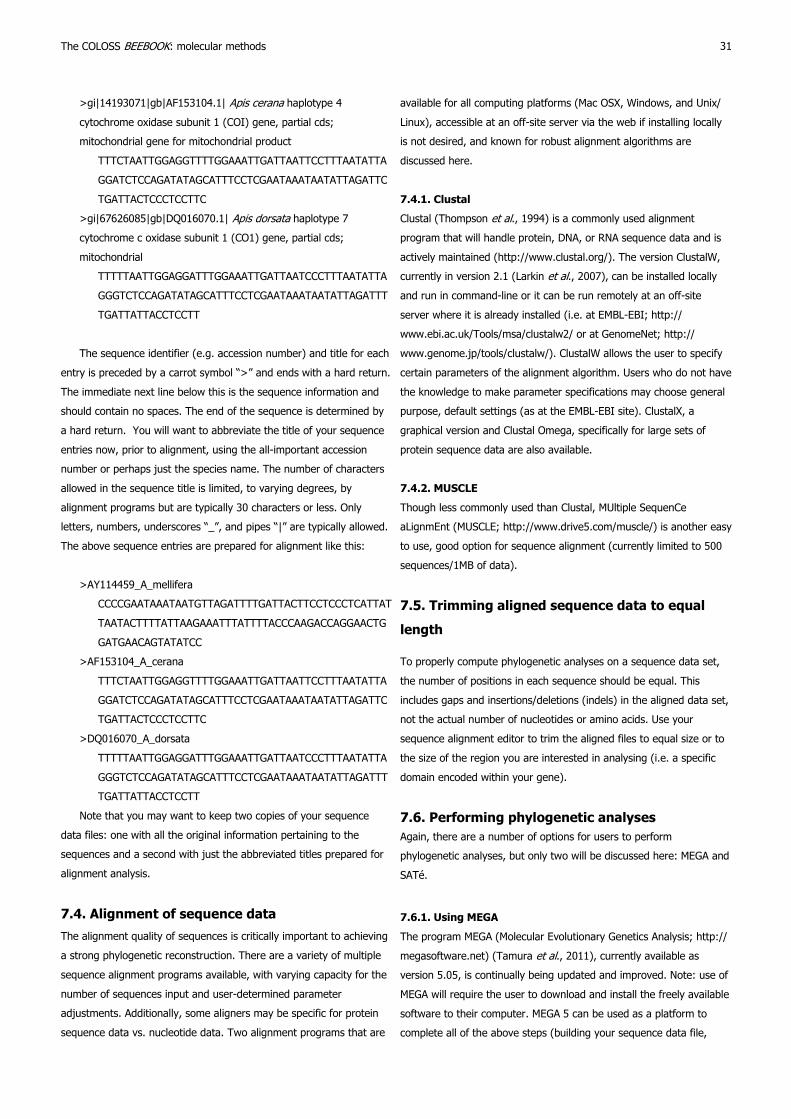
>gi|14193071|gb|AF153104.1| Apis cerana haplotype 4

cytochrome oxidase subunit 1 (COI) gene, partial cds;

mitochondrial gene for mitochondrial product

TTTCTAATTGGAGGTTTTGGAAATTGATTAATTCCTTTAATATTA

GGATCTCCAGATATAGCATTTCCTCGAATAAATAATATTAGATTC

TGATTACTCCCTCCTTC

>gi|67626085|gb|DQ016070.1| Apis dorsata haplotype 7

cytochrome c oxidase subunit 1 (CO1) gene, partial cds;

mitochondrial

TTTTTAATTGGAGGATTTGGAAATTGATTAATCCCTTTAATATTA

GGGTCTCCAGATATAGCATTTCCTCGAATAAATAATATTAGATTT

TGATTATTACCTCCTT

The sequence identifier (e.g. accession number) and title for each

entry is preceded by a carrot symbol “>” and ends with a hard return.

The immediate next line below this is the sequence information and

should contain no spaces. The end of the sequence is determined by

a hard return. You will want to abbreviate the title of your sequence

entries now, prior to alignment, using the all-important accession

number or perhaps just the species name. The number of characters

allowed in the sequence title is limited, to varying degrees, by

alignment programs but are typically 30 characters or less. Only

letters, numbers, underscores “_”, and pipes “|” are typically allowed.

The above sequence entries are prepared for alignment like this:

>AY114459_A_mellifera

CCCCGAATAAATAATGTTAGATTTTGATTACTTCCTCCCTCATTAT

TAATACTTTTATTAAGAAATTTATTTTACCCAAGACCAGGAACTG

GATGAACAGTATATCC

>AF153104_A_cerana

TTTCTAATTGGAGGTTTTGGAAATTGATTAATTCCTTTAATATTA

GGATCTCCAGATATAGCATTTCCTCGAATAAATAATATTAGATTC

TGATTACTCCCTCCTTC

>DQ016070_A_dorsata

TTTTTAATTGGAGGATTTGGAAATTGATTAATCCCTTTAATATTA

GGGTCTCCAGATATAGCATTTCCTCGAATAAATAATATTAGATTT

TGATTATTACCTCCTT

Note that you may want to keep two copies of your sequence

data files: one with all the original information pertaining to the

sequences and a second with just the abbreviated titles prepared for

alignment analysis.

7.4. Alignment of sequence data

The alignment quality of sequences is critically important to achieving

a strong phylogenetic reconstruction. There are a variety of multiple

sequence alignment programs available, with varying capacity for the

number of sequences input and user-determined parameter

adjustments. Additionally, some aligners may be specific for protein

sequence data vs. nucleotide data. Two alignment programs that are

The COLOSS BEEBOOK: molecular methods 31

available for all computing platforms (Mac OSX, Windows, and Unix/

Linux), accessible at an off-site server via the web if installing locally

is not desired, and known for robust alignment algorithms are

discussed here.

7.4.1. Clustal

Clustal (Thompson et al., 1994) is a commonly used alignment

program that will handle protein, DNA, or RNA sequence data and is

actively maintained (http://www.clustal.org/). The version ClustalW,

currently in version 2.1 (Larkin et al., 2007), can be installed locally

and run in command-line or it can be run remotely at an off-site

server where it is already installed (i.e. at EMBL-EBI; http://

www.ebi.ac.uk/Tools/msa/clustalw2/ or at GenomeNet; http://

www.genome.jp/tools/clustalw/). ClustalW allows the user to specify

certain parameters of the alignment algorithm. Users who do not have

the knowledge to make parameter specifications may choose general

purpose, default settings (as at the EMBL-EBI site). ClustalX, a

graphical version and Clustal Omega, specifically for large sets of

protein sequence data are also available.

7.4.2. MUSCLE

Though less commonly used than Clustal, MUltiple SequenCe

aLignmEnt (MUSCLE; http://www.drive5.com/muscle/) is another easy

to use, good option for sequence alignment (currently limited to 500

sequences/1MB of data).

7.5. Trimming aligned sequence data to equal

length

To properly compute phylogenetic analyses on a sequence data set,

the number of positions in each sequence should be equal. This

includes gaps and insertions/deletions (indels) in the aligned data set,

not the actual number of nucleotides or amino acids. Use your

sequence alignment editor to trim the aligned files to equal size or to

the size of the region you are interested in analysing (i.e. a specific

domain encoded within your gene).

7.6. Performing phylogenetic analyses

Again, there are a number of options for users to perform

phylogenetic analyses, but only two will be discussed here: MEGA and

SATé.

7.6.1. Using MEGA

The program MEGA (Molecular Evolutionary Genetics Analysis; http://

megasoftware.net) (Tamura et al., 2011), currently available as

version 5.05, is continually being updated and improved. Note: use of

MEGA will require the user to download and install the freely available

software to their computer. MEGA 5 can be used as a platform to

complete all of the above steps (building your sequence data file,

Fig. 3. Phylogenetic reconstruction of cytochrome oxidase I gene

from Apis and Bombus species (Hymenoptera; Apidae) using

Neighbour-Joining method (A) and Maximum Likelihood (B). Topology

of each was tested with 1,000 bootstrap iterations (consensus tree is

shown) using Nasonia vitripennis (Hymenoptera; Pteromalidae) as

outgroup. Scale represents the substitution rate per site from a total

of 981 positions. A) was computed using Maximum Composite

Likelihood (Tamura et al., 2004) with uniform rates among sites and

pairwise gap deletion. B) was computed using Tamura-Nei model

(Tamura and Nei, 1993) with uniform rates at all sites.

alignment using Clustal or MUSCLE, and trimming sequence data). It

gives the user the ability to construct phylogenies using distance

based (i.e. Neighbour Joining) and character based (i.e. Maximum

Likelihood) methods (see Table 1) and test them using bootstrapping.

It also includes a tree viewer that allows for some editing of the final

output tree and many additional features not covered here.

7.6.1.1. Converting data to MEGA format

Before phylogenetic tests can be run on your sequence data file, it

must be converted into a format that MEGA can read, the *.meg file

format.

1. From the ‘File’ menu in MEGA, select ‘Convert File Format to

MEGA…’, browse to your alignment file, select ‘FASTA format’

from the ‘Data Format’ pull down menu, then select ‘OK’.

2. A window will open asking for you to specify a name and

location for the newly created *.meg file.

The new file will be created and opened under a tab in the same

window next to your open FASTA format file.

3. MEGA will warn you to check the file for any errors and

adjustments to your *.meg file can be made in this window

and saved.

Details about the *.meg format are available in MEGA.

7.6.1.2. Constructing and testing phylogenetic trees

Described below is a basic, distance based Neighbour-Joining analysis

using bootstrap statistical tests for robustness (Felsenstein, 1985).

1. From the main MEGA window, open the ‘Phylogeny’ pull down

tab and select ‘Construct/Test Neighbour-Joining Tree’.

2. Browse to and open the .meg file you just created. Select the

appropriate data type (nucleotide or protein sequence data).

Note the defaults for missing data, alignment gaps and identity and

make any changes if necessary then select ‘OK’.

3. A window will open asking you to identify your sequence data

as protein-coding or not.

4. Another window will open asking for genetic code selection.

For the example, provided here, using the cytochrome oxidase I (COI)

gene, select ‘Invertebrate Mitochondrial’.

5. A third window opens and allows you to select a number of

parameters for your analysis.

A minimum of 100 and typically 1,000 iterations of bootstrapping are

used to test the robustness of your phylogeny. For now, we will

accept the default parameters for our simple analysis.

6. A progress window will open for you until the test is

completed.

7. When complete, a window opens with two tabs showing the

‘Original tree’ generated, as well as a ‘Bootstrap consensus

tree’, which is the tree you should refer to.

Bootstrap support values show the percentage of iterations supporting

the shown topology.

32 Evans et al.

8. The tree image can be saved as a pdf for good resolution for

presentation (Fig. 3A), can be saved as a mts Tree Session

File for future viewing in MEGA, or exported and saved as a

more general Newick (.nwk) format file that is readable by a

variety of other tree viewing programs (e.g. FigTree http://

tree.bio.ed.ac.uk/software/figtree/ ; TreeDyn http://

www.treedyn.org/).

For comparison, a Maximum Likelihood (ML) analysis of the same

alignment was performed in a similar manner and is shown in Fig. 3B.

7.6.2. Using SATé

An alternative software package to MEGA for ML analyses is SATé

(Simultaneous Alignment and Tree estimation; Liu et al., 2012), which

infers sequence alignment and tree building concurrently as an

iterative process using the ML method. This program must also be

downloaded for use, and is currently freely available as SATé-II at

http://phylo.bio.ku.edu/software/state/sate.html. The user experience

for SATé is still being improved, including recommendations for how

to parse phylogenetic runs. A strength of SATé is that it accepts up to

1,000 sequences in the FASTA format as described in section 7.3.,

and claims speed and precision in phylogenetic analyses. Through

changes in subproblem size parameters (below) it is possible to run

SATé on desktop machines, but using this software on high-memory

and high-CPU clusters will be simpler since those parameters will be

less likely to affect performance. Several alignment programs are

bundled with the download, including Clustal and MUSCLE. If an

alignment is already prepared, SATé will use Randomized a(x)-

elerated Maximum Likelihood (RaxML) (Satmatakis, 2006) to infer an

initial tree for phylogeny reconstruction.

From the main SATé window, select the desired analysis criteria in

the following sections:

7.6.2.1. External tools

SATé breaks the tree topology down into subproblems during each

round of analysis and realigns the data for each subset, merges the

alignments into a full alignment and re-estimates the tree for full

alignment.

1. ‘Aligner’ is used to select the multiple sequence alignment tool

to produce the initial full alignment.

2. ‘Merger’ is used to select the multiple sequence alignment tool

to merge the alignments of subproblems into a bigger and

final multiple sequence alignment.

3. ‘Tree estimator’ uses RAxML for tree estimation with the

chosen evolutionary ‘Model’.

7.6.2.2. Sequence import and tree building

1. Click ‘Sequence file…’ to upload your sequence alignment file

in FASTA format (Note: the file MUST have the extension

*.fas or *.fasta to be read by SATé; see section 7.3.).

2. Select the appropriate ‘Data Type’ (nucleotide or amino acid).

3. If you have previously generated a ‘Tree file’, you can upload

it as the initial guide for SATé, if appropriate.

7.6.2.3. Job Settings

1. Specify the ‘Job Name’ for identifying output files created by

SATé.

2. Select the folder/directory for storing the created outfile files

using ‘Output Dir.’

The COLOSS BEEBOOK: molecular methods 33

7.6.2.4. SATé Settings

This section allows users to control the details of the algorithm. In

each iteration, the dataset will be breaking down into non-overlapping

sequence subproblems and these subproblems are given to the

chosen alignment tool.

1. There are options under ‘Quick Set’ to allow a more or less

intensive search during the SATé iterative process.

2. ‘Max. Subproblem’ is used to control the largest dataset that

are aligned during the iterative process.

3. Use the ‘Fraction’ option to express the maximum problem

size as a percentage of the total number of taxa in the full

dataset.

This value will be limited by available computational power.

4. Use the ‘Size’ option for size cutoff in absolute number of

sequences.

5. Select ‘Decomposition’ to choose how the process should be

broken to create subproblems.

6. ‘Apply Stop Rule’ is used to control how SATé should be

finished.

The decision to stop can be done based on number of iterations (one

may be sufficient), the amount of time in hours or ‘Blind Mode

Enabled’ meaning that SATé will terminate if it ever completes one

iteration without improving the ML score.

7. Click ‘Start’ to run the SATé analysis.

There will be five files created in the selected directory after SATé

is completed. An alignment file (*.aln), tree file (*.tre), best ML score

file (*.score), error file (*.err) and history file (*.out). Unlike MEGA,

SATé does not have bundled tree viewing or alignment viewing

programs, so the user will need to open the tree file using one of the

tree viewing programs described above and the alignment file using

Clustal or a similar alignment viewing program. The other files can be

opened with a text editor (i.e. Notepad, TextEdit). In addition, SATé

does not utilize bootstrap testing to support inferred tree topology.

Rather, a similarity score from 0-1 (0 is most similar and 1 is least

similar) is placed on the branches to aid in topology interpretation.

Hence, other reconstruction methods should be compared to confirm

the output.

7.6.3. Building trees using distance and character based

methods

To assess the reliability of the tree topology, users should be aware of

the phylogenetic tree construction and tree analysis methods

according to the data and algorithmic strategy used. Each method has

different assumptions that may or may not be valid for the

evolutionary process of the given sequence data. For example, the

distance based method UPGMA (Unweighted Pair Group Method with

Arithmetic mean) assumes a neutral mutation rate proportional to

time (a molecular clock). Therefore, it is important to be aware of this

Table 1. Classification of phylogenetic analysis methods and strategies.

fact when evaluating tree topology generated by each method. It is

encouraged that one run a variety of distance based methods

(Neighbour-Joining, UPGMA, Minimum Evolution) that calculate

evolutionary distance between sequences, and character based

methods (Maximum Parsimony, Maximum Likelihood, Bayesian) that

determine the most probable evolutionary event history between

sequences (Table 1).

Statistical testing of topology should also be performed where

possible, i.e. bootstrapping analysis. Altering the substitution model,

rates and patterns, and treatment of gaps/missing data may also be

warranted, though the varying justifications for each of these tests is

beyond the detail provided here. Low branch support for any topology

shown in the final tree or conflicts in topology determined by multiple

testing should be addressed when presenting any phylogenetic data.

8. Genomic resources and tools

8.1. Introduction

Genomic analyses take several forms. At one level, any study that

draws inferences for protein-coding genes or other genetic traits in

the context of their neighbors on chromosomes is ‘genomic’. More

recently, genomic studies are those that use massive DNA sequencing

strategies to describe and piece together entire sections of the

targeted genome, without using PCR or other selective techniques to

target specific short regions. Ultimately, genomic studies hope to

assemble chromosome-length stretches of an organism’s genetic

blueprint, and then annotate or describe the functionality of specific

regions within chromosomes. The field of genomics is driven by

technological advances, including huge cost reductions for the

sequencing of samples and advances in both statistical methods and

computational resources for analysing the obligatory large datasets.

Current estimates indicate that entire pipelines (sets of routines

needed for an output analysis) are viable for only six months before

becoming obsolete. One helpful review of modern techniques is given

by Desai et al. (2012) and there are numerous advances and tutorials

available via the forums Seqanswers.com and the GALAXY wiki

34 Evans et al.

(http://wiki.galaxyproject.org/FrontPage). Researchers are advised to

consult these sources while planning genomic, transcriptomic, and

metagenomic projects, as the standards and possible analyses are

improving constantly.

8.2. Honey bee genome project

After a multi-year international project, the honey bee genome was

described in fall, 2006, in a main overview paper (Honey bee Genome

Sequencing Consortium, 2006) and > 30 satellite genome-enabled

companion papers (primarily in the journals Insect Molecular Biology

and Genome Research). Sequence data, generated using dideoxy

sequencing was assembled into ca. 10,000 contigs (blocks of

overlapping sequence reads) spanning ca. 238 million base pairs.

These contigs are in many cases linked together by scaffolding (a

strategy whereby long strands of DNA are sequenced from each end

and linked via informatics) leading to an assembly that was > 95%

complete for the non-repetitive genome. Honey bee genes and

various genomic features are predicted based on homology to other

organisms, evidence from RNA expression studies, and evidence for

open reading frames. The current genome assembly along with a

consensus (“GLEAN”) gene set and other resources are available at

“Beebase” (www.beebase.org/, Christine Elsik, Univ. Missouri) and at

the U.S. National Institutes of Health National Center for

Biotechnology Information (http://www.ncbi.nlm.nih.gov/genome?

term=apis%20mellifera). Both sites allow for downloading sequences

as well as searching the genome via the BLAST family of search

algorithms, while the Beebase site also provides the chance to

‘browse’ the genome visually. Efforts are continuing to improve the

primary Apis mellifera genome data while adding sequence data from

different honey bee strains.

8.3. Honey bee parasite and pathogen genomes

Most of the named RNA viruses for honey bees have been sequenced

and published. These genomes are relatively small and tend to be

placed into the NCBI databases upon publication (http://

www.ncbi.nlm.nih.gov/genomes/GenomesGroup.cgi?taxid=439488).

Genome sequences for several parasites and pathogens with larger

genomes (e.g., Paenibacillus larvae, Ascosphaera apis, Nosema

ceranae, and the mite Varroa destructor; (Qin et al., 2006; Cornman

et al., 2009; Cornman et al., 2010; Chan et al., 2011) are held at the

NCBI as well as at Beebase and can be queried there alongside the

above honey bee genome data.

8.4. Comparative genomics

Currently, assembled genome sequences exist for over 30 insects and

other arthropods, and that number is soon to increase dramatically

(http://arthropodgenomes.org/wiki/i5K). Resources that have proven

useful for comparing honey bee genes to those found in other insects

(e.g., to Drosophila and other insects for which gene function is firmly

Tree building strategy Method

Distance based Character based

Clustering algorithm UPGMA

Neighbour Joining n/a

Optimality criterion Minimum Evolution

Maximum Parsimony

Maximum Likelihood

Bayesian Analysis

decided) include the NIH-NCBI and the OrthoDB database run from

the University of Geneva (http://cegg.unige.ch/orthodb5). In addition,

as each incarnation of the honey bee genome is published, annotations

based on presence/absence and functional similarity to other insects

is simultaneously added. With projects on four other Apis species

underway, along with social and solitary apoid bees, strategies for

comparative genomics will be in flux for some time. The orthoDB

database, along with flybase (www.flybase.org) are good places to

start for insights from comparative genomics, and each site has hosts

the requisite tools (gene searching/alignment/retrieval) for carrying

out comparative analyses.

8.5. Second-generation sequencing

Initial genome projects, from small viruses through the human and

honey bee project, all relied on ‘Sanger’ dideoxy sequencing, a

relatively expensive but accurate protocol developed in the 1980’s

that generates sequences (often drawn from random cloned fragments

for the popular ‘shotgun’ sequence method) of several hundred to

1000 base pairs. Since 2000, there has been a great economization of

sequencing, such that current technologies are more than ten-fold

less expensive than Sanger sequencing. Nevertheless, Sanger

sequencing persists and is often the right strategy when compared to

newer technologies (which currently give either quite short or quite

inaccurate sequences). Readers should consider ILLUMINA/SOLEXA

sequencing (summarized in the methylation section 11. below), 454

pyrosequencing, SOLiD sequencing or the Ion Torrent platform (all

platforms are reviewed by Metzger, 2010), and the final decision

might rest on local availability along with different strengths of each

platform. As of 2012, most DNA and RNA sequencing efforts include

at least some component of ILLUMINA sequencing, as that technology

is viewed as being most cost-effective.

8.6. Genomic sequence assembly

Standards and tools for genome sequence assembly and analysis are

constantly improving and the best strategy for carrying out a genome

project is often through collaboration or through mimicking the

protocols and computational strategies used by a recent genome

project of similar scope (genome size, budget for sequencing and

informatics, etc.). Accordingly, we will not list specific pipelines for

these processes, but can direct researchers to sites such as http://

www.broadinstitute.org/scientific-community/science/programs/

genome-sequencing-and-analysis/computational-rd/computational-,

http://bioinformatics.igm.jhmi.edu/salzberg/Salzberg/Software.html,

and http://soap.genomics.org.cn/soapdenovo.html. Of these options,

whole-genome assemblies using the ALLPATHS-LG method (the first

link above for the Broad Institute) have been highly successful for

both microbes and higher organisms, and this method is arguably the

tool of choice currently.

The COLOSS BEEBOOK: molecular methods 35

8.7. Transcriptomic analyses (“RNASeq”)

Transcriptomic analyses are helpful for seeing trends in honey bee

gene expression as well as changes due to experimental conditions,

and bee researchers have carried out such studies for many years,

adapting as new methods arise. Two recent papers have used the

ILLUMINA platform for studying gene regulation in response to

nutrition (Alaux et al., 2011) and responsiveness to varroa mites and

viruses (Nazzi et al., 2012), respectively. Analyzing RNASeq data will

depend on the sequencing platform as well as developments in

software and public or personal computational resources, all of which

are under constant renewal. Generally, RNASeq experiments rely on

differential gene expression (DGE) between categories of one factor

(e.g., bees exposed to mites versus controls) and the statistical

analysis identifies which regions are up- or down-regulated in the

context of this factor. Nazzi et al., 2012 used a technique prescribed

by Mortazavi et al., (2008) that, like all current methods, first

develops a model for how often a particular expressed region should

be seen in a sequencing effort, and then uses the number of times

that sequence was sampled to determine whether it was up-or down

regulated compared to an expected level. There are now numerous

such methods and both methods and strategies to trim the

computational resources for their use are being improved monthly.

Public platform with video tutorials for RNASeq analysis that promises

to remain current is described at the Galaxy site (https://

main.g2.bx.psu.edu/).

8.8. Metagenomics

Metagenomic approaches began as an attempt to study the functional

significance of all organisms in a habitat, and the term was first used

to describe soil microbes and their collective proteins (Handelsman

et al., 1998). In honey bees, usage has so far focused on identifying

pathogen taxa (Cox-Foster et al., 2007; Runckel et al., 2011, Cornman

et al., 2012) and, more recently, on targeted surveys of bacterial

associates in honey bee guts (Martinson et al., 2011; Mattila et al.,

2012). There are six key decision points in metagenomic surveys and,

rather than choose any specific recipe, we will instead list those

decisions and their outcomes:

8.8.1. RNA versus DNA sampling

RNA pools contain those genomes that are actively producing proteins

AND genomes of the key RNA viruses in bees. RNA sampling is often

used for assessing bee pathogens. DNA sampling is preferable when

samples are poorly preserved (given the higher stability of DNA) and

as a means of reducing the often overwhelmingly high frequency of

ribosomal RNA’s (75-80%) in most sequenced RNA samples.

8.8.2. Sample preparation

Both RNA and DNA destined for metagenomic surveys can be

extracted using the means described in sections 3 and 4 (e.g. Trizol®

extractions for RNA and CTAB extractions for DNA). For more

recalcitrant samples (e.g. spore stages, or samples of organisms with

impermeable coats, common to bacterial species and fungi) it is

important to use mechanical or enzymatic rupturing of the cell coat

via proteinase K, as described in the above CTAB DNA extraction

protocol (section 3.2.1.), or prolonged shaking with a suspension of

low-affinity silica particles or other inert solids.

8.8.3. Amplicon-based or shotgun sequencing

Given the low costs of sequencing, it is feasible now to simply survey

all nucleic acids in a sample and then assign them to taxa in various

kingdoms via searches of local or online databases. Nevertheless,

targeted deep sequencing of specific taxonomic groups can benefit

from a selection of specific regions via PCR-based amplification prior

to generating the sequencing libraries. This has been done most

frequently with the 454 sequencing platform since relatively long read

lengths on this platform (> 400 bp) enable the capture of sequence

data for a substantial section of the targeted species. Several studies

have now used amplicon-based sequencing to describe bacterial

populations carried by honey bees. As with any PCR protocol, this

approach will under sample taxa with mismatches to the initial primer

sequences since no PCR primers are truly ‘universal’ to a targeted

group. Nevertheless, there are many examples of primers that amplify

broadly across all of the major bacterial taxonomic groups, and

amplicon-based 454 sequencing has appears to provide a consistent

and accurate view of bacterial communities in bees. The software

environment Qiime (http://qiime.org/) is widely used to match

amplicon-based sequences to microbial databases in order to identify

and quantify taxa.

8.8.4. Assembly of shotgun sequences vs. read mapping

For sequences generated by shotgun sequencing, it is generally

desirable to assemble all sequencing reads into contigs (aggregates of

nearly identical sequences from the same region and species) prior to

statistical analysis, since this can reduce computational needs greatly

while retaining vital statistics including the number of reads per

contig. Once the computationally intensive assembly of contigs has

taken place (using for example the Metavelvet routine, http://

metavelvet.dna.bio.keio.ac.jp/) datasets can be reduced by many

orders of magnitude. This is critical if online or ‘cloud’ databases are

searched for microbial matches since the data transfer speeds alone

for such searches can be measured in days when using raw sequence

36 Evans et al.

reads. In addition, contigs are by definition longer than any individual

read and therefore also can provide a more secure match to distant

taxa. The count data for sequenced reads per contig provides the

measure of depth that, once scaled to contig length, allows estimates

of microbial frequency. Once metagenomic sequences have been

assembled, moderate experiments can often be enacted without cost

to the user at public resources such as GALAXY (https://main.g2.bx.psu.edu/).

As with any complicated statistical procedure it is highly possible to

get erroneous matches and statistical results, and researchers are

advised to enlist the help of colleagues with current expertise here.

In practice, metagenomic analyses are also carried out by

mapping (aligning with high probability) individual sequence reads to

members of a reference database, and algorithms (including Tophat,

http://genomics.jhu.edu/software.html) have been developed that are

extremely efficient at doing so. For diagnostic regions with highly

conserved sequences (e.g., parts of the rRNA operons) both

assembling and mapping are problematic and query sequences often

cannot be placed securely to even family-level matches. In this case,

it is best to bin sequences at a higher taxonomic level (even Order)

rather than force matches into a possibly erroneous taxon.

Nevertheless, as genome sequencing of microbial species is increasing

exponentially, even rare and distant taxa tend to have a fully

sequenced family member in the public databases, as described below

in section 8.8.5.

8.8.5. Databases for metagenomics

Several sites have emerged for mapping metagenomic sequence reads

and amplicons, including the longstanding Ribosomal Database Project

for bacterial and archael 16S alignments (http://rdp.cme.msu.edu/),

the SILVA databases for rRNA’s generally (http://www.arb-silva.de/),

and MEGAN (ab.inf.uni-tuebingen.de/software/megan/), which aspires

to map to targets across the tree of life. Each site allows for limited

web searching, and for downloading relevant databases for more

efficient local searches.

8.8.6. Post-assignment statistics

Quantifying differences between two or more samples in the taxa to

which reads or contigs map is the ultimate goal for many metagenomic

experiments. While not the only option, MG-RAST (metagenomics.anl.gov/)

provides an example of statistical comparisons using read mapping.

Assuming read accounts are normalized by size of their target (various

methods have been used for this), and then the count frequencies

themselves can be used with a variety of standard statistics. Similarly,

Qiime, mentioned above in section 8.8.3, provides an effective way

for mapping reads to microbial taxa.

9. Fluorescence In Situ

Hybridization (FISH) analysis of

tissues and cultured cells

9.1. Introduction

Fluorescence in situ Hybridization (FISH) is a sensitive and specific

method for localizing expressed genes or microbes within tissues of

the honey bee. In general, a probe matching a specific DNA or RNA

sequence is exposed to prepared tissues. This probe can then be

localized using fluorescent tags, pointing the researcher to the precise

location of a desired target. To date this method has been used

successfully to show the locations of bacterial associates of bees

(Martinson et al., 2012, Yue et al., 2008, and below).

9.2. Tissue fixation and tissue sectioning

exemplified with gut tissue

1. Immobilize about 20 bees with CO2.

2. Cut of the head.

3. Fix the abdomen on a separation plate with micro pins.

4. Remove carefully the alimentary tract of each bee with

forceps.

5. Transfer the hindgut and the midgut into one well of a 24-well

microtiter plate.

6. Fix tissues in 4% formalin (Roth) for 24 hours at 4°C by

shaking.

The further embedding and blocking procedure using e.g. Technovit

8100 and Technovit 3040 kits (Heraeus-Kulzer) should be performed

as given in the manufacturer´s protocols (Heraeus-Kulzer, T8100

embedding kit).

7. Wash the alimentary tracts with 6.8% sucrose in 1xphosphate

buffered saline (1xPBS, pH 7.0) for 24 hours at 4°C.

8. For dehydration transfer the tissue in 100% acetone for one

hour.

9. Pre-infiltrate the organs with T8100 basic-solution and 100%

acetone (mixed 1:1) for two hours.

10. Prepare the infiltration solution (0.6 g hardener I in 100 ml

T8100 basic solution).

11. Transfer the organs into the infiltration solution.

12. Incubate at 4°C for at least 24 hours and up to one week,

depending on tissue size.

13. Apply careful shaking for better infiltration results.

14. Prepare the embedding solution (mix 0.5 ml hardener II with

15 ml infiltrating solution).

15. Fill the mould of a Teflon-embedding form (pre-cooled at -20° C)

with the embedding solution.

16. Transfer the tissue and orientate it in the mould.

17. Close the well immediately with a plastic strip.

The COLOSS BEEBOOK: molecular methods 37

18. Incubate at 4°C for 3 hours to allow polymerization.

19. Finally, block the polymerized probes with histoblocs and with

the Technovit 3040 kit (both from Heraeus-Kulzer) using the

manufacturer´s protocol.

20. Prepare semi thin-sections (2-4 µm) with a rotation microtome

(Leica).

Use a knife with a hard metal edge (Tungsten).

21. For fluorescence in situ-hybridization transfer the tissue

sections on Polysine™-covered glass slides (Fisher Scientific,

Menzel-Gläser).

9.3. Fixation of cultured cells grown in

suspension

1. Transfer 100 µl of cultured cells into a cell funnel-chamber of

a cell spin (Tharmac).

2. Centrifuge the cells with 600 rpm (54xg) gently for 5 minutes

on a glass slide (VWR).

3. Remove the cell funnel-chamber.

4. Let the medium air dry.

5. Fix the cells in 4% formalin (Roth) at 4°C for 24 hours.

9.4. FISH-analysis of tissue sections and fixed

insect cells

1. Wash the slides (tissue sections and fixed insect cells) twice in

1xPBS.

2. For further processing, transfer each slide into a 10 ml dish.

3. Add 10 ml of 1 µg ml-1 Proteinase K in Proteinase K-buffer

(0.2 M Tris-HCl, pH 7.5).

4. Transfer the dish into a humid chamber (Eppendorf,

Thermostat Plus) for 5 min at 37°C.

5. Remove the Prot K and wash each slide with 10 ml of 1xPBS.

6. For post-fixation add 10 ml of 4% formalin (Roth).

7. Incubate at RT for 20 min.

8. Aspirate the formalin.

9. Remove remaining solution by washing the slides three times

with 1xPBS-buffer.

10. Prepare hybridization buffer:

200 µl of 100% formamide,

180 µl 5 M NaCl,

20 µl 1 M Tris/HCl,

1 µl 10% SDS,

599 µl DEPC-H2O, pre-warm to 46°C in a heating block.

11. Add the probes to 37.5 µl pre-warmed (46°C) hybridization

buffer:

7.5 µl species-specific probe annealing to a region of the 16S

rRNA or another species-specific genomic region of the

pathogen to be detected labelled with fluorescein

isothiocyanate-FITC with a final concentration of 15 ng µl-1.

Sequence of Nosema spp.-probes: Gisder et al. (2011); sequence of

DWV-probe: Möckel et al. (2011); sequence of P. larvae-probe: Yue

et al. (2008)

5 µl Euk516-probe (5‘-ACCAGACTTGCCCTCC-3‘, universally

detecting eukaryotic ribosomes by hybridizing to a universal

conserved sequence of the eukaryotic 18S rRNA) labelled with

sulforhodamine 101 acid chloride-Texas Red® with a final

concentration of 10 ng µl-1.

12. Continue incubation in the heating block which is now covered

with a lid (i.e. incubation at 46°C in the dark).

13. Cover the slides with LifterSlips (VWR).

14. Pipette 50 µl of hybridization buffer to each slide (tissue

sections or fixed cells).

15. Transfer the slide into a hybridization chamber (Corning,

Corning chamber), drop 15 µl H2O into the given wells to

preserve the humidity.

16. Close the chamber tightly.

17. Put the corning chamber in a 46°C water bath for overnight

hybridization.

18. Open the hybridization chamber and remove the cover slips in

1xPBS.

19. Wash the slides three times with 1xPBS.

20. Let them air dry.

21. Stain the nuclei with 50 µl 4′, 6-Diamidin-2-phenylindol-

(DAPI, 1 µg ml-1 in 99% methanol) solution for 10 min in the

dark.

22. Wash the slides again three times with 1xPBS.

23. Let them air dry.

24. Cover the slides with the ProLong Gold antifade reagent

(Invitrogen) and a cover slip (Roth).

25. Analyse the tissue sections and the cells under an inverse

fluorescence microscope (e.g. Nikon, Ti-Eclipse) at 100-fold and 600-

fold magnification using consecutively a FITC-, TexasRed- and DAPI-

filter.

10. RNA interference

10.1. Introduction

RNA interference (RNAi) is a cellular mechanism leading to a knock-

down of gene expression mediated by target specific double-stranded

RNA (dsRNA) molecules (Fire et al., 1998). Understanding the

mechanism of mRNA destruction by these dsRNA molecules

dramatically increased the possibilities of functional genomics studies

during the last decade especially in organisms where the recovery of

mutants is not feasible. Thus RNAi has become a dominant reverse

genetic method for the study of gene functions and furthermore, plays

an increasing role in therapeutics and in pest control (Maori et al., 2009;

Liu et al., 2010; Hunter et al., 2010).

38 Evans et al.

Up to now a dozen studies report on the successful usage of RNAi in

honey bees. But the application methods and also the choice of RNAi

effective molecules are very diverse. Several studies report on the

application of dsRNA to eggs and larvae whether by injection

(Aronstein and Salivar, 2005; Beye et al., 2002; Maleszka et al., 2007)

or ingestion (Aronstein et al., 2006; Patel et al., 2007; Kucharski

et al., 2008; Nunes and Simoes, 2009; Liu et al., 2010). Others report

on a successful manipulation of adult bees (Amdam et al., 2003;

Farooqui et al., 2004; Seehuus et al., 2006; Schlüns and Crozier,

2007; Maori et al. 2009; Paldi et al., 2010; Mustard et al., 2010;

Jarosch and Moritz, 2011; Jarosch et al., 2011).

This section aims at a collection of RNAi protocols successfully

applied in honey bees beforehand. The well-established protocols for

producing dsRNA as well as siRNA (short interfering RNAs, the

products of dsRNA once the enzyme Dicer and its partners have

processed them) molecules are presented. Moreover, the two

application methods feeding and injection are presented and

compared to each other. In conclusion, we summarize five important

factors that may decrease the effectiveness of target gene expression

knock-down.

10.2. Production of RNA interfering molecules

10.2.1. siRNA design and synthesis

So far most bee scientists have used dsRNA rather than siRNA for

RNAi experiments. Although dsRNA molecules have advantages in

handling, off-target effects (Jarosch et al., 2012) have been reported

in honey bees. Therefore the usage of siRNAs is recommended where

feasible. This allows the selection of one or a few short sequences to

initiate RNAi, rather than the many tens of possible permutations

generated by a typical dsRNA construct, any of which might cause

effects away from the desired target.

1. Design 3-6 siRNAs for your target gene in order to find an

optimal siRNA.

General guidelines for siRNA design:

siRNA targeted sequence is usually 21 nt in length.

Avoid regions within 50-100 bp of the start codon and the

termination codon.

Avoid intron regions.

Avoid stretches of 4 or more bases such as AAAA, CCCC.

Avoid regions with GC content < 30% or > 60%.

Avoid repeats and low complex sequence.

Avoid single nucleotide polymorphism (SNP) sites.

Perform BLAST homology search to avoid off-target

effects on other genes or sequences (16- to 18-nt–long

stretches of homology are suggested as the maximum

acceptable length in RNAi studies per Ambion siRNA

design guidelines).

Design negative controls by scrambling the target siRNA

sequence. This control RNA has the same length and

nucleotide composition as the target specific siRNA but in

a different order. Make sure that the scrambled siRNA

does not show homologies for any known bee gene.

Several web based programs for appropriate siRNA design, which

implement the actual siRNA design algorithms, are available

(e.g. siRNA target designer version 1.6 (Promega); siDesign center

(Dharmacon, Inc); Block-iTTM RNAi Designer (Invitrogen).

2. Use T7 RibomaxTM Express RNAi System (Promega) for siRNA

production.

1. Follow the manufacturers´ instructions.

2. Incubation time may be increased in order to increase the

siRNA yield (A time-course experiment has to be

performed beforehand in order to find the optimal

incubation time).

3. Assess the quality and quantity by photometric measurements

(OD260) and by capillary gel electrophoresis (alternatively

agarose gel electrophoresis, see section 3.2.1).

10.2.2. Production of dsRNA

Since dsRNAs can cause off-target effects, you need to be careful in

designing them. Nevertheless, RNAi efforts using dsRNA constructs

have proven effective in honey bees. To avoid targets that might

interfere with other honey bee genes, you need to compare your

sequence with the honey bee genome during the design process using

the Basic Local Alignment Tool (www.ncbi.nlm.nih.gov). Make sure

none of the designed dsRNAs has 20-bp segments identical to any

known bee sequence. As dsRNAs are processed by the dicer complex

into a cocktail of siRNAs 19–21 nt in length, the absence of 20-nt

stretches of homology minimizes the possibility of off-target effects.

1. Use the E-RNAi web application (Horn and Boutros, 2010) for

optimal dsRNA design.

Design of dsRNA sequences has to be stringent in order to avoid/

minimize off-target effects.

2. Set up appropriate negative controls.

Note: be careful using GFP; this sequence might cause off-target

effects in some cases (GenBank ID: U17997, Clontech; Jarosch

and Moritz, 2012).

Other possible negative controls: e.g., Q-marker (Beye et al., 2002).

3. Amplify the chosen target fragment by using target specific T7

(TAA TAC GAC TCA CTA TAG GGC GAT) added primer in

optimized PCRs using approximately 100-ng genomic DNA

obtained by chloroform– phenol extraction (e.g. Maniatis

et al., 1982).

The COLOSS BEEBOOK: molecular methods 39

4. Clone the amplified fragments into pGem-T easy vectors

(Promega) according to the manufacturer’s instructions.

(Cloning eliminates the possibility of a dsRNA mixture due to a

polymorphism of the PCR product).

5. Transform your plasmids into JM109 competent cells

(Promega) following the instructions from the manufacturer.

6. Prepare the plasmids according to Del Sal (1988).

7. Analyse the identity of the cloned sequence by Sanger

sequencing.

8. Once the right clone has been identified its insert needs to be

amplified to serve as a template for dsRNA production by

standard PCR using again T7 tailed primers.

8.1. E.g. use Biotherm DNA Polymerase (Genecraft); chemicals:

0.2 mM dNTPs,

0.3 µM of T7-promotor added primer,

5 U Taq Polymerase,

in a total reaction volume of 100 µl.

8.2. PCR protocol:

5 min DNA denaturation, and Taq activation, at 95°C,

40 cycles of:

95°C for 30 sec,

x°C (primer specific annealing temperature) 30 sec,

72°C for 1 min.

A final extension of 20 min at 72°C completes the

protocol.

9. Purify the PCR-products with the QIAquick® PCR Purification

Kit (Qiagen).

10. Use the T7 RibomaxTM Express RNAi System (Promega) for

dsRNA production.

Time course experiments and experiments for optimizing the

incubation temperature have to be conducted beforehand (e.g.

Jarosch et al., 2011 used an extended transcription time of 5 h at 32°C).

11. Purify the dsRNA by a Trizol® (Invitrogen) - chloroform-

treatment following the manufacturers´ instructions.

12. Resolve the pellet in nuclease free water.

13. Assess the dsRNA quality and quantity photometrically and by

agarose gels or capillary gel electrophoresis.

The photometric measurement of the OD260/OD280 ratio should be

between 1.8 and 2. A lower ratio indicates contamination with

proteins. As a contamination with DNA or dsRNA degradation cannot

be detected by photometry, visualization of the dsRNA product is

necessary. For this 1.5% agarose gels can be used, see section

3.2.1). A single distinct band should be visible.

14. Adjust dsRNA concentrations to 5 µg/µl by diluting with insect

ringer (54 mM NaCl; 24 mM KCl; 7 mM CaCl2 x 2H2O) right

before the injection.

10.3. RNAi Applications

10.3.1. RNAi in adult honey bees via feeding

1. Take newly emerged bees (1-2 d old) from one colony from

one brood frame.

2. Set up at least two controls:

1. Bees fed with 50% sugar water alone.

2. Bees fed with scrambled siRNA (siRNA with exactly the

same nucleotides as the target siRNA but in an altered

order lacking any similarity with other known bee genes).

3. Take a mixture of two siRNAs specific for the target gene.

Note: in previous experiments a mixture of two siRNAs was more

effective than single siRNAs (Jarosch et al., 2011).

4. Put 35-40 newly emerged bees in wooden cages (see the

BEEBOOK paper on maintaining adult honey bees in vitro

under laboratory conditions (Williams et al., 2013)) supplied

with a small comb and pollen ad libitum.

5. Put cages in temperature controlled incubators (see the

BEEBOOK paper on maintaining adult honey bees in vitro

under laboratory conditions (Williams et al., 2013)) and feed

with 1.5 ml 50% sugar water containing approximately 1 µg

siRNA per insect every 24 hours.

6. Dependent on the actual experiments bees can be held for

several weeks.

7. Once the experiment is finished, bees should be shock-frozen

in liquid nitrogen in order to maintain the RNA status.

10.3.2. RNAi in honey bee larvae via feeding

1. Take a comb with second instar larvae out of the colony.

2. Transfer it to the lab.

The whole treatment is conducted at room temperature.

3. Draw a map of the different treatment groups on the very

same comb for future identification of the treated individuals.

4. Apply 1 µl of sugar solution containing the respective amount

of dsRNA directly into the cells. Deposit it at the bottom of the

worker brood cell that contains a drop of food. Avoid touching

the larvae. Successful experiments used dsRNA concentrations

between 0.5 µg (Nunes and Simões, 2009) and up to 1.26 µg

(Aronstein et al., 2006).

In addition to the first dsRNA feeding you may feed another µg of

your dsRNA after 12 hours. This feeding cycle can be repeated for

several days (Liu et al., 2010) until the life stage of interest is reached.

5. Place the comb back to its host colony two hours after

treatment and take samples at the life stage you are

interested in.

40 Evans et al.

10.3.3. Gene knock-down by abdominal injection of target-

specific dsRNA/siRNA

RNA interfering molecules injected by intra-abdominal injection do

not reach every tissue (Jarosch and Moritz, 2011). But especially the

fat body can be easily reached by this user friendly method (Amdam

et al., 2003; Jarosch and Moritz, 2011).

1. Take age-defined workers (see the BEEBOOK paper on

miscellaneous methods (Human et al., 2013)).

Note: newly emerged workers are a little bit more difficult to inject as

their abdomen is quite flexible.

2. Immobilise bees by cooling down in at 4°C.

3. Fix the bees on wax plates using small fixing pins.

4. Inject 5 µg of freshly diluted dsRNA or alternatively 3 µg of

freshly diluted siRNA (treatment and control dsRNA/siRNA)

between the 5th and 6th abdominal segment using a 10 µl

microsyringe (e.g. Hamilton).

5. Inject negative controls with insect ringer (54 mM NaCl;

24 mM KCl; 7 mM CaCl2 x 2H2O).

6. Keep the injected workers on wax plates until they recover

and keep bees not showing haemolymph leakage (visible on

their substrate or as a droplet on the cuticle) together with

about 25 nurse bees (1-10 days) in cages (see the BEEBOOK

paper on maintaining adult honey bees in vitro under

laboratory conditions (Williams et al., 2013)).

7. Sacrifice the bees by shock-freezing in liquid nitrogen.

8. Store them at -80°C until tissue preparation.

9. Prepare the worker tissues on cooled wax plates using an RNA

Stabilization Reagent (e.g. RNAlater®) in order to avoid RNA

degradation.

10.4. Concluding remarks

Based on the literature (see Huvenne and Smagghe, 2012 for review)

five aspects seem to be most important to conduct successful RNAi

knockdown experiments in honey bees.

Concentration of dsRNA: For every target gene the most effective

concentration of RNAi molecules has to be determined. It does not

follow the general rule: The more the better. Nunes and Simões (2009)

for example report on the removal of 2nd instar larvae, which were fed

with 3 and 5 µg dsRNA. In contrast, larvae fed with just 0.5 µg dsRNA

did not show a significant higher removal rate than the control group,

and moreover exhibited an mRNA silencing effect of about 90%.

Nucleotide sequence: Sequences of the RNAi effective molecules

have to be carefully designed and tested in order to avoid off-target

effects.

Length of the dsRNA fragment: When not using siRNAs the length of

the dsRNA fragments may be crucial for uptake and efficient silencing.

Most experiments used dsRNA ranging from 300 to 520 bp (see

Huvenne and Smagghe, 2012 for review). Moreover, a minimal length

of 211 bp is suggested in S2 cells (Saleh et al., 2006).

Honey bee life stage: Although adults are easier to handle,

literature of other insects suggest a larger silencing effect in younger

life stages. E.g. in fall armyworms (Spodoptera frugiperda) the

silencing effects after RNAi treatment were reported to be less

effective than in S. frugiperda larvae (Griebler et al., 2006). Thus the

usage of larvae rather than adults where feasible may be advisable in

honey bees as well.

Application method: The two application methods presented here

both have pros and cons. The feeding regimes lead to an individually

different consumption of food and therefore to the ingestion of

different dosages of dsRNA. But in contrast to injections protocols,

feeding is much easier in handling and moreover, it causes less stress

in the target animals. Moreover, studies suggest, that the composition

of the target tissue may have some influence on the accessibility of

dsRNA when choosing injection as application method (Jarosch and

Moritz, 2011).

11. DNA methylation in honey bees

11.1. Introduction

Methylation of chromosomal DNA is a flexible epigenetic mechanism

that plays a critical role in gene regulation, and patterns of

methylation across the genome are often surrogates for interesting

sets of proteins that are regulated in concert with each other and with

biological traits. In order to detect methylated bases in genomic DNA

(essentially only cytosines are methylated), DNA has to be treated

with bisulfite to convert non-methylated cytosines to uracil and

subsequently to thymine during the PCR amplification step.

11.2. DNA methylation in honey bees

So far, four full methylomes (genome-wide methylation patterns)

have been generated for Apis mellifera using the following tissues:

adult brains of queens and workers and 96 hrs-old queen and worker

larval heads (Lyko et al., 2010; Foret et al., 2012). The below protocol

describes methylation analyses of DNAs extracted from the dissected

brains of 50 age matched active queens and 50 8-day old workers

(dissection of clean, gland-free brains is shown at: http://

dl.dropbox.com/u/59152790/Brain%20dissection%20Maleszka%

20lab.wmv).

A similar protocol was used to generate larval methylomes (Foret

et al., 2012) and in principle this procedure should work for any bee

tissue and/or life stage from which intact RNA’s can be extracted as

below (section 11.3.).

The COLOSS BEEBOOK: molecular methods 41

11.3. DNA extraction from various tissues for

methylation analysis

Methylation analyses do not depend on a particular DNA extraction

method. Nevertheless, the below extraction has been validated in a

variety of honey bee tissues.

1. Homogenize tissues in a 1.5 ml microcentrifuge tube in a

small volume of NTE buffer:

100 mM NaCl,

50 mM Tris pH 8.2,

10 mM EDTA,

1% SDS,

Proteinase K (500 µg per ml, freshly dissolved).

2. Add a small amount (0.01%) of a non-ionic detergent such as

Triton X100.

The detergent is beneficial (increases the efficiency of proteinase K

digestion), but not necessary.

3. Add more buffer (roughly 500 µl per 20-50 mg of tissue).

4. Incubate at 55°C for 1-3 hrs.

5. Extract with 1 volume of phenol: chloroform.

6. Spin for 10 min at 10,000rpm.

7. Collect the upper phase (repeat the extraction if the upper

phase looks cloudy).

8. Add 1 µl of RNase A (10 mg/ml).

9. Incubate for 10 min at 370C to digest RNA.

This step is not necessary for bisulfite conversion, but the

presence of RNA interferes with measuring DNA yield.

10. Precipitate DNA with 1 volume of isopropanol or 2 volumes of

EtOH.

11. Spin gently (5,000 rpm for 2 min).

12. Discard the supernatant.

13. Wash the pellet once with 70% EtOH.

14. Remove ethanol, but DO NOT DRY THE PELLET!

15. Dissolve the pellet in TE buffer by heating to 65°C.

16. Store at 4°C (or at -80°C for long term storage).

Clean DNA preps are stable at 4°C for at least 5 years. The majority

of DNA strands from the above prep are 200-250 kb in length with the

smallest molecules around 70 kb.

Note: DNA preps from larvae might appear milky after this

procedure, but such preps are suitable for bisulfite conversions.

Alternatively use the MasterPure DNA Purification kit from AMRESCO

(Cat. No. MCD85201) yields cleaner larval preps.

11.4. High-throughput sequencing of targeted

regions

11.4.1. Fragmentation of DNA

1. Fragment 5µg of high molecular weight DNA using the Covaris

S2 AFA System in a total volume of 100µl.

Fragmentation-run parameters:

Duty cycle 10%,

Intensity: 5,

Cycles/burst: 200,

Time: 3min,

Number of cycles: 3,

This results in a total fragmentation-time of 180s.

2. Confirm fragmentation with a 2100 Bioanalyzer (Agilent

Technologies) using a DNA1000 chip, aiming for fragment

sizes of 140 bp on average for both queen and worker DNAs.

11.4.2. End-repair of sheared DNA

Having a blunt (neither strand longer than the other) end to each

double-stranded DNA section is needed to attach the below adaptors

(‘handles’ that help connect DNA during library formation), and this is

achieved as follows:

1. Concentrate fragmented DNA to a final volume of 75 µl using

a DNA Speed Vac.

2. End-repair fragmented DNA in a total volume of 100 µl using

the Paired End DNA Sample Prep Kit (Illumina, PE-102-1001)

following manufacturer’s protocol.

11.4.3. Adaptor ligation

Ligate adaptors using the Illumina Early Access Methylation Adaptor

Oligo Kit (P/N: 1006132) and the Paired End DNA Sample Prep Kit

(Illumina, PE-102-1001), as recommended by the manufacturer.

11.4.4. Size selection of adapter-ligated fragments

For the size selection of the adaptor-ligated fragments use the E-Gel

Electrophoresis System (Invitrogen) and a Size Select 2% precast

agarose gel (Invitrogen) as below.

1. Load each fragmented DNA on two lanes of an E-gel.

2. Electrophorese using the “Size Select” program for 16 min.

3. Using a size standard (50 bp DNA Ladder, Invitrogen, Cat no.

104 16-014), extract 240 bp fragments from the gel.

4. Pool samples and directly transfer to bisulfite treatment

without further purification.

11.4.5. Bisulfite conversion and amplification of the final

library

1. Bisulfite treatment can be carried out with the EZ-DNA

Methylation Kit (Zymo) as recommended by the manufacturer,

with the exception of a modified thermal profile for the

bisulfite conversion reaction. Alternatively the QIAGEN EpiTect

42 Evans et al.

Bisulfite Kit can be used.

The conversion is carried out in a thermal cycler using the

following thermal profile:

15 cycles of:

95° C for 15 sec,

50° C for 1hr,

Incubate at 4° C for at least 10 min.

2. Amplify the resulting libraries using the Fast Start High Fidelity

PCR System (Roche, 03 553 400 001) with buffer 2, the

Illumina PE1.1 and PE2.1 amplification primers, and the below

protocol.

PCR thermal profile:

95°C- 2min,

11 cycles of:

95°C for 30 sec,

65°C for 20 sec,

72°C for 30 sec,

72°C for 7 min,

20°C hold.

3. Purify products on PCR purification columns (MinElute,

Qiagen), eluting in 20 µl elution buffer (Qiagen).

11.4.6. Validation of the libraries

1. Analyse 1 µl of the libraries on a 2100 Bioanalyzer (Agilent

Technologies) using a DNA1000 chip.

2. Confirm product size of ca. 240 base pairs and adequate

quantity using the DNA1000 size standards.

11.4.7. Sequencing and data analysis

1. Use a Solexa Genoma Analyzer GAIIx with a v2 Paired End

Cluster Generation Kit - GA II (Illumina, PE-203-2001) and v3

36 bp Cycle Sequencing Kits (Illumina, FC-104-3002) following

manufacturer’s protocols, for sequencing.

2. Extract sequences using Illumina Pipeline v1.4 software.

3. Perform image analysis and base calling using Illumina SCS

v2.5 software.

8 pM of material is used per sequence lane, generating between 10

and 16M sequence reads.

11.5. Mapping and methylation assessment

1. Trim the above sequence data using the Illumina Data

Analysis Pipeline.

2. Align bisulfite-converted sequencing reads to the honey bee

genome using the BSSeeker software (http://

pellegrini.mcdb.ucla.edu/BS_Seeker/BS_Seeker.html) as

described in Foret et al. (2012); http://www.pnas.org/

content/suppl/2012/03/12/1202392109.DCSupplemental/

pnas.201202392SI.pdf#nameddest=STXT.

3. Reads containing consecutive CHN nucleotides are the

product of incomplete bisulfite conversion and must first be

discarded.

4. To increase the accuracy of methylation calls, only those

cytosines fulfilling neighbourhood quality standards are

counted (bases of quality 20 or more, flanked by at least

three perfectly matching bases with a PHRAP quality score of

15 or more).

5. The methylation status of each cytosine base can be modelled

by a binomial distribution with the number of trial equal to the

number of mapping reads and the probability equal to the

conversion rate.

6. A base is called methylated if the number of reads supporting

a methylated status departed from this null model significantly

at the 5% level after correcting for multiple testing.

7. Differentially methylated genes are identified using

generalized linear models of the binomial family; the response

vector CpGmeth (number of methylated and non-methylated

reads for each CpG in a gene) was modelled as a function of

two discrete categorical variables, the caste and the CpG

position: CpGmeth = caste * CpGi.

8. P-values are corrected for multiple testing using the Benjamini

and Hochberg method. These tests are carried out using the

R statistical environment (http://www.r-project.org).

9. Honey bee ESTs and predicted genes are loaded into a Mysql

database and visualized with Gbrowse, where CpG

methylation levels in queens and workers are added as

separate tracks.

11.6. Methylation dynamics and expression of

individual genes

Targeted analyses of selected genes can be conducted using 454

sequencing of amplified gene fragments from bisulfite-converted

DNAs. For a small-scale testing the amplicons can be cloned into a

plasmid, cloned and sequenced using via Sanger dideoxy sequencing

(Foret et al., 2009). Both approaches can be used to validate genome

-wide methylation data, but 454 sequencing allows for a much higher

coverage, as shown in section 8.5.

11.6.1. Amplicon sequence selection

1. Illumina sequencing and BSMAP mapping results can be

confirmed by 454 sequencing of a set of bisulfite amplicons.

2. Specific amplicon sequences are selected using raw

methylome data and the following arbitrary criteria:

1. Minimum coverage - 5 mapped reads for each queen and

worker sample.

The COLOSS BEEBOOK: molecular methods 43

2. Minimum 2 methylated CpGs within a region of ~400-600 bp of

sequence showing at least 50% difference in methylation

levels between the two samples. This selection is very

stringent, but assures that amplicons with high probability of

differential methylation are selected.

3. In addition a few regions of mtDNA that is not methylated are

selected as controls (optional).

11.6.2. Bisulfite DNA conversion

1. The Qiagen EpiTect Bisulfite Kit and the manufacture’s

protocol is widely accepted as the most efficient and reliable

kit for DNA conversion. The amount of starting materials can

range from 0.1 to 2 μg.

2. Because DNA conversion with bisulfite is only ~98% efficient

it is highly recommendable to repeat this protocol twice.

3. 1/10th of the second conversion reaction is sufficient for

subsequent amplification.

11.6.3. Bisulfite PCR

Bisulfite amplicons are amplified using a nested PCR protocol (Wang

et al., 2006; Foret et al., 2009). Nested primers contained an

additional 9 nucleotide-long linkers with EcoRI or HindIII recognition

sequences allowing directional cloning of the amplicons.

PCR reactions are performed in 25 µl volume containing:

1x PCR buffer,

mM MgCl2,

mM dNTP,

50 pmol each forward and reverse primer,

5 units Taq polymerase.

Reaction efficiencies are optimized via annealing temperature

gradients (Mastercycler gradient PCR machine, Eppendorf) and testing

multiple Taq polymerases such as GoTaq (Promega) or FastStart Taq

(Roche).

Cycling profile is as follows:

Initial denaturation at 940C for 2 min,

Followed by 40 cycles of:

15 sec denaturation at 940C,

15 sec annealing at primer-specific optimal temperature,

60 sec extension at 720C,

A final extension cycle at 720C for 5 min.

When using FastStart Taq polymerase, the denaturation

temperature was increased to 950C, initial denaturation time to 5 min

and cycling denaturation and annealing times to 30 sec.

11.7. RNA extraction

1. RNA for analysis can be extracted using the TRIzol®/QIAGEN

RNeasy combination method followed by the QIAGEN Mini or

Rneasy Minelute Cleanup kit, or by the detailed protocol in the

RNA methods section 4.3. above.

2. RNA concentrations are then evaluated via Nanodrop (section

3.2.1) analyses and integrity assessed by gel electrophoresis

(see section 4.4.).

11.8. cDNA synthesis and template quantification

1. Typical first-strand reactions consist of a 20µ volume

containing:

0.5-2 mg of total RNA, or 50-100 ng of poly(A)RNA,

100 pmol of anchored d(T)20VN primer,

200 units of Superscript III (Invitrogen),

1X concentration of proscribed buffer.

2. The tube is incubated for 1 h at 50°C.

3. Terminate by adding 30 µl of TE buffer and freezing.

4. Resulting cDNAs can be screened for levels of specific genes

via quantitative-PCR as described in the RNA methods in

section 4.7.

12. Acknowledgements

We thank four careful reviewers and Editors Peter Neumann and

Vincent Dietemann for their insights and advice. The COLOSS

(Prevention of honey bee COlony LOSSes) network aims to explain

and prevent massive honey bee colony losses. It was funded through

the COST Action FA0803. COST (European Cooperation in Science and

Technology) is a unique means for European researchers to jointly

develop their own ideas and new initiatives across all scientific

disciplines through trans-European networking of nationally funded

research activities. Based on a pan-European intergovernmental

framework for cooperation in science and technology, COST has

contributed since its creation more than 40 years ago to closing the

gap between science, policy makers and society throughout Europe

and beyond. COST is supported by the EU Seventh Framework

Programme for research, technological development and

demonstration activities (Official Journal L 412, 30 December 2006).

The European Science Foundation as implementing agent of COST

provides the COST Office through an EC Grant Agreement. The

Council of the European Union provides the COST Secretariat. The

COLOSS network is now supported by the Ricola Foundation - Nature

& Culture.

44 Evans et al.

13. References AGÜERO, M; SAN MIGUEL, E; SÁNCHEZ, A; GÓMEZ-TEJEDOR, C;

JIMÉNEZ-CLAVERO, M A (2007) A fully automated procedure for

the high-throughput detection of avian influenza virus by real-time

reverse transcription–polymerase chain reaction. Avian Diseases

51: 235–241. http://dx.doi.org/10.1637/7634-042806R1.1

ALAUX, C; DANTEC, C; PARRINELLO, H; LE CONTE, Y (2011)

Nutrigenomics in honey bees: Digital gene expression analysis of

pollen's nutritive effects on healthy and varroa-parasitized bees.

BMC Genomics 12: 496.

http://dx.doi.org/doi:10.1186/1471-2164-12-496

AMDAM, G; SIMOES, Z; GUIDUGLI, K; NORBERG, K; OMHOLT, S

(2003) Disruption of vitellogenin gene function in adult honey

bees by intra-abdominal injection of double-stranded RNA. BMC

Biotechnology 3: 1. http://dx.doi.org/doi:10.1186/1472-6750-3-1.

ARONSTEIN, K; PANKIW, T; SALDIVAR, E (2006) SID-1 is implicated

in systemic gene silencing in the honey bee. Journal of Apicultural

Research 45(1): 20-24.

ARONSTEIN, K; SALDIVAR, E (2005) Characterization of a honey bee

toll related receptor gene am18w and its potential involvement in

antimicrobial immune defense. Apidologie 36(1): 3-14.

http://dx.doi.org/10.1051/apido:2004062

BECKER, C; HAMMERLE-FICKINGER, A; RIEDMAIER, I; PFAFFL, M W

(2010) mRNA and microRNA quality control for RT-qPCR analysis.

Methods 50: 237-243.

http://dx.doi.org/10.1016/j.ymeth.2010.01.010

BECKER, S; FRANCO, J R; SIMARRO, P P; STICH, A; ABEL, P M;

STEVERDING, D (2004) Real-time PCR for detection of

Trypanosoma brucei in human blood samples. Diagnostic

Microbiology and Infectious Disease 50(3): 193-199.

http://dx.doi.org/ 10.1016/j.diagmicrobio.2004.07.001

BEYE, M; HÄRTEL, S; HAGEN, A; HASSELMANN, M; OMHOLT, S W

(2002) Specific developmental gene silencing in the honey bee

using a homeobox motif. Insect Molecular Biology 11(6): 527-532.

BIRCH, L; ENGLISH, C A; BURNS, M; KEER, J T (2004) Generic

scheme for independent performance assessment in the

molecular biology laboratory. Clinical Chemistry 50(9): 1553-1559.

http://dx.doi.org/10.1373/clinchem.2003.029454

BRUUN-RASMUSSEN, T; UTTENTHAL, Å; HAKHVERDYAN, M; BELÁK, S;

WAKELEY, P R; REID; S M; EBERT, K; KING, D P (2009)

Evaluation of automated nucleic acid extraction methods for virus

detection in a multicenter comparative trial. Journal of Virological

Methods 155: 87–90.

http://dx.doi.org/DOI:10.1016/j.jviromet.2008.09.021

BUSTIN, S A (2000) Absolute quantification of mRNA using real-time

reverse transcription polymerase chain reaction assays. Journal of

Molecular Endocrinology 25(2): 169-193.

http://dx.doi.org/10.1677/jme.0.0250169

BUSTIN, S A; BEAULIEU, J F; HUGGETT, J; JAGGI, J; KIBENGE, R;

FSBOLSVIK, P A; PENNING, L C; TOEGEL, S (2010) MIQE précis:

Practical implementation of minimum standard guidelines for

fluorescence-based quantitative real-time PCR experiments. BMC

Molecular Biology 11: e74.

http://dx.doi.org/10.1186/1471-2199-11-74

BUSTIN, S A; BENES, V; GARSON, J A; HELLEMANS, J; HUGGETT, J;

KUBISTA, M; MUELLER, R; NOLAN, T; PFAFFL, M W; SHIPLEY, G L;

VANDESOMPELE, J; WITTWER, C T (2009) The MIQE Guidelines:

minimum information for publication of quantitative Real-Time

PCR experiments. Clinical Chemistry 55(4): 611-622.

http://dx.doi.org/10.1373/clinchem.2008.112797

BUSTIN, S A; NOLAN, T (2004) Pitfalls of quantitative real-time

reverse-transcription polymerase chain reaction. Journal of

Biomolecular Techniques 15(3): 155-166.

CAETANO-ANOLLES, G (1998) DAF optimization using Taguchi

methods and the effect of thermal cycling parameters on DNA

amplification. Biotechniques 25(3): 472-6, 478-80.

CANDOTTI, D; TEMPLE, J; OWUSU-OFORI, S; ALLAIN, J P (2004)

Multiplex real-time quantitative RT-PCR assay for hepatitis B virus,

hepatitis C virus, and human immunodeficiency virus type 1.

Journal of Virological Methods 118(1): 39-47.

http://dx.doi.org/10.1016/j.jviromet.2004.01.017

CHAISOMCHIT, S; WICHAJARN, R; JANEJAI, N;

CHAREONSIRIWATANA, W (2005) Stability of genomic DNA in

dried blood spots stored on filter paper. Southeast Asian Journal

of Tropical Medicine and Public Health 36(1): 270-273

CHAMOLES, N A; NIIZAWA, G; BLANCO, M; GAGGIOLI, D;

CASENTINI, C (2004) Glycogen storage disease type II: enzymatic

screening in dried blood spots on filter paper. Clinica Chimica Acta

347(1-2): 97-102.

http://dx.doi.org/10.1016/j.cccn.2004.04.009

CHAN, Q; CORNMAN, R S; BIROL, I; LIAO, N; CHAN, S; DOCKING, T

R; JACKMAN, S; TAYLOR, G; JONES, S; DE GRAAF, D; EVANS, J;

FOSTER, L (2011) Updated genome assembly and annotation of

Paenibacillus larvae, the agent of American foulbrood disease of

honey bees. BMC Genomics 12(1): 450

http://dx.doi.org/10.1186/1471-2164-12-450.

CHANTAWANNAKUL, P; WARD, L; BOONHAM, N; BROWN, M (2006)

A scientific note on the detection of honey bee viruses using real-

time PCR (TaqMan) in varroa mites collected from a Thai honey

bee (Apis mellifera) apiary. Journal of Invertebrate Pathology 91

(1): 69-73. http://dx.doi.org/10.1016/j.jip.2005.11.001

CHEADLE, C; VAWTER, M P; FREED, W J; BECKER, K G (2003)

Analysis of microarray data using Z score transformation. Journal

of Molecular Diagnostics 5(2): 73-81.

http://dx.doi.org/10.1016/S1525-1578(10)60455-2

The COLOSS BEEBOOK: molecular methods 45

CHEN, Y P; EVANS, J; HAMILTON, M; FELDLAUFER, M (2007) The

influence of RNA integrity on the detection of honey bee viruses:

molecular assessment of different sample storage methods.

Journal of Apicultural Research 46(2): 81-87.

http://dx.doi.org/10.3896/IBRA.1.46.2.03

CHEN, Y P; HIGGINS, J A; FELDLAUFER, M F (2005a) Quantitative real

-time reverse transcription-PCR analysis of deformed wing virus

infection in the honey bee (Apis mellifera L.). Applied and

Environmental Microbiology 71(1): 436-441.

http://dx.doi.org/10.1128/AEM.71.1.436-441.2005

CHEN, Y P; PETTIS, J S; FELDLAUFER, M F (2005b) Detection of

multiple viruses in queens of the honey bee Apis mellifera L.

Journal of Invertebrate Pathology 90(2): 118-121.

http://dx.doi.org/10.1016/j.jip.2005.08.005

CHEN, Y P; SMITH, I B; COLLINS, A M; PETTIS, J S; FELDLAUFER, M F

(2004b) Detection of deformed wing virus infection in honey bees,

Apis mellifera L., in the United States. American Bee Journal 144:

557-559.

CHEN, Y; ZHAO, Y; HAMMOND, J; HSU, H T; EVANS, J D;

FELDLAUFER, M F (2004) Multiple virus infections in the honey

bee and genome divergence of honey bee viruses. Journal of

Invertebrate Pathology 87: 84-93.

http://dx.doi.org/10.1016/j.jip.2004.07.005

CHERNESKY, M; JANG, D; CHONG, S; SELLORS, J; MAHONY, J (2003)

Impact of urine collection order on the ability of assays to identify

Chlamydia trachomatis infections in men. Sexually Transmitted

Diseases 30(4): 345-347.

http://dx.doi.org/10.1097/00007435-200304000-00014

CORNMAN, R S; CHEN, Y P; SCHATZ, M C; STREET, C; ZHAO, Y;

DESANY, B; EGHOLM, M; HUTCHISON, S; PETTIS, J S; LIPKIN, W I;

EVANS, J D (2009) Genomic analyses of the microsporidian

Nosema ceranae, an emergent pathogen of honey bees. PLoS

Pathogens 5(6): e1000466,

http://dx.doi.org/10.1371/journal.ppat.1000466

CORNMAN, R S; SCHATZ, M C; JOHNSTON, J S; CHEN, Y P; PETTIS, J;

HUNT, G; BOURGEOIS, L; ELSIK, C; ANDERSON, D; GROZINGER, C M;

EVANS, J D (2010) Genomic survey of the ectoparasitic mite Varroa

destructor, a major pest of the honey bee Apis mellifera. BMC

Genomics 11: 602. http://dx.doi.org/10.1186/1471-2164-11-602

CORNMAN, R S; TARPY, D R; CHEN, Y-P; JEFFREYS, L; LOPEZ, D;

PETTIS, J S; VANENGELSDORP, D; EVANS, J D (2012) Pathogen

webs in collapsing honey bee colonies. PloS One e43562.

http://dx.doi.org/10.1371/journal.pone.0043562

CORONA, M; HUGHES, K A; WEAVER, D B; ROBINSON, G E (2005)

Gene expression patterns associated with queen honey bee

longevity. Mechanisms of Ageing and Development 126(11): 1230

-1238. http://dx.doi.org/10.1016/j.mad.2005.07.004

COX-FOSTER, D L; CONLAN, S; HOLMES, E C; PALACIOS, G; EVANS, J D;

MORAN, N A; QUAN, P L; BRIESE, T; HORNIG, M; GEISER, D M;

MARTINSON, V; VANENGELSDORP, D; KALKSTEIN, A L;

DRYSDALE, A; HUI, J; ZHAI, J; CUI, L; HUTCHISON, S K;

SIMONS, J F; EGHOLM, M; PETTIS, J S; LIPKIN, W I (2007) A

metagenomic survey of microbes in honey bee Colony Collapse

Disorder. Science 318(5848): 283-287.

http://dx.doi.org/10.1126/science.1146498

DAINAT, B; EVANS, J D; CHEN, Y P; NEUMANN, P (2011) Sampling

and RNA quality for diagnosis of honey bee viruses using

quantitative PCR. Journal of Virological Methods 174(1-2): 150-

152. http://dx.doi.org/10.1016/j.jviromet.2011.03.029

DE LA RÚA, P; JAFFÉ, R; DALL´OLIO, R; MUÑOZ, I; SERRANO, J

(2009) Biodiversity, conservation and current threats to European

honey bees. Apidologie 40: 263–284.

http://dx.doi.org/10.1051/apido/2009027

DE MIRANDA, J R; BAILEY, L; BALL, B V; BLANCHARD, P; BUDGE, G;

CHEJANOVSKY, N; CHEN, Y-P; GAUTHIER, L; GENERSCH, E;

DE GRAAF, D; RIBIÈRE, M; RYABOV, E; DE SMET, L VAN DER

STEEN, J J M (2013) Standard methods for virus research in Apis

mellifera. In V Dietemann; J D Ellis; P Neumann (Eds) The

COLOSS BEEBOOK, Volume II: standard methods for Apis

mellifera pest and pathogen research. Journal of Apicultural

Research 52(4): http://dx.doi.org/10.3896/IBRA.1.52.4.22

DE MIRANDA, J R (2008) Diagnostic techniques for virus detection in

honey bees. In Aubert, M F A; Ball, B V; Fries, I; Moritz, R F A;

Milani, N; Bernardinelli, I (Eds). Virology and the honey bee. EEC

Publications; Brussels, Belgium. pp 121-232.

DE MIRANDA, J R; FRIES, I (2008) Venereal and vertical transmission

of deformed wing virus in honey bees (Apis mellifera L.). Journal

of Invertebrate Pathology 98: 184-189.

http://dx.doi.org/10.1016/j.jip.2008.02.004

DEL SAL, G; MANFIOLETTI, G; SCHNEIDER, C (1988) A one-tube

plasmid DNA mini-preparation suitable for sequencing. Nucleic

Acids Research 16: 20.

DESAI, N; ANTONOPOULOS, D; GILBERT, J A; GLASS, E M; FOLKER, F

(2012) From genomics to metagenomics. Current Opinion in

Biotechnology. 23(1): 72-76.

DIETEMANN, V; NAZZI, F; MARTIN, S J; ANDERSON, D; LOCKE, B;

DELAPLANE, K S; WAUQUIEZ, Q; TANNAHILL, C; FREY, E;

ZIEGELMANN, B; ROSENKRANZ, P; ELLIS, J D (2013) Standard

methods for varroa research. In V Dietemann; J D Ellis; P

Neumann (Eds) The COLOSS BEEBOOK, Volume II: standard

methods for Apis mellifera pest and pathogen research. Journal of

Apicultural Research 52(1):

http://dx.doi.org/10.3896/IBRA.1.52.1.09

EDGAR, R C (2004) MUSCLE: multiple sequence alignment with high

accuracy and high throughput. Nucleic Acids Research 32: 1792-

1797. http://dx.doi.org/10.1093/nar/gkh340

46 Evans et al.

ERALI, M; SCHMIDT, B; LYON, E; WITTWER, C (2003) Evaluation of

electronic microarrays for genotyping factor-V, factor-II and

MTHFR. Clinical Chemistry 49(5): 732-739.

http://dx.doi.org/10.1373/49.5.732

ESTOUP, A; SOLIGNAC, M; HARRY, M; CORNUET, J M (1993)

Characterization of (GT)n and (CT)n microsatellites in two insect

species Apis mellifera and Bombus terrestris. Nucleic Acids

Research 21: 1427-1431.

EVANS, J D (1993) Parentage analyses in ant colonies using simple

sequence repeat loci. Molecular Ecology 2: 393-397.

EVANS, J D (2004) Transcriptional immune responses by honey bee

larvae during invasion by the bacterial pathogen, Paenibacillus

larvae. Journal of Invertebrate Pathology 85(2): 105-111.

http://dx.doi.org/10.1016/j.jip.2004.02.004

EVANS, J D (2006) Beepath: An ordered quantitative-PCR array for

exploring honey bee immunity and disease. Journal of

Invertebrate Pathology 93(2): 135-139.

http://dx.doi.org/10.1016/j.jip.2006.04.004

EVANS, J D; WHEELER, D E (2000) Expression profiles during honey

bee caste determination. Genome Biology 2(1):

http://dx.doi.org/10.1186/gb-2000-2-1-research0001

EVANS, J D; WHEELER, D E (2001) Gene expression and the evolution

of insect polyphenisms. Bioessays 23(1): 62-68.

http://dx.doi.org/10.1002/1521-1878(200101)

FAROOQUI, T (2004) Octopamine receptors in the honey bee (Apis

mellifera) brain and their disruption by RNA-mediated

interference. Journal of Insect Physiology 50(8): 701-713.

http://dx.doi.org/10.1016/j.jinsphys.2004.04.014

FELSENSTEIN, J D (1985) Confidence limits on phylogenies: An

approach using the bootstrap. Evolution 39: 783-791.

FIEVET, J; TENTCHEVA, D; GAUTHIER, L; DE MIRANDA, J R;

COUSSERANS, F; COLIN, M E; BERGOIN, M (2006) Localization of

deformed wing virus infection in queen and drone Apis mellifera L.

Virology Journal 3: e16. http://dx.doi.org/10.1186/1743-422X-3-16

FIORINI, G S; CHIU, D T (2005) Disposable microfluidic devices:

fabrication, function, and application. Biotechniques 38(3): 429-

446. http://dx.doi.org/10.2144/05383RV02

FIRE, A; XU, S; MONTGOMERY, M K; KOSTAS, S A; DRIVER, S E;

MELLO, C C (1998) Potent and specific genetic interference by

double-stranded RNA in Caenorhabditis elegans. Nature 391

(6669): 806-811.

http://dx.doi.org/URLhttp://dx.doi.org/10.1038/35888

FIXE, F; CHU, V; PRAZERES, D M; CONDE, J P (2004) An on-chip thin

film photodetector for the quantification of DNA probes and

targets in microarrays. Nucleic Acids Research 32(9): e70.

http://dx.doi.org/10.1093/nar/gnh066

FLEIGE, S; PFAFFL, M W (2006) RNA integrity and the effect on the

real-time qRT-PCR performance. Molecular Aspects of Medicine

27: 126-139. http://dx.doi.org/10.1016/j.mam.2005.12.003

FORET, S; KUCHARSKI, R; PELLEGRINI, M; FENG, S; JACOBSEN, S E;

ROBINSON, G E; MALESZKA, R (2012). DNA methylation

dynamics, metabolic fluxes, gene splicing, and alternative

phenotypes in honey bees. Proceedings of the National Academy

of Sciences of the United States of America 109(13): 4968- 4973.

http://dx.doi.org/10.1073/pnas.1202392109

FRIES, I (1997) Protozoa, In Morse, R A; Flottum, K (Eds). Honey bee

pests, predators, & diseases (3rd edition). A I Root: Medina, Ohio,

USA. pp 57-76.

GARNERY, L; SOLIGNAC, M; CELEBRANO, G; CORNUET, J-M (1993) A

simple test using restricted PCR-amplified mitochondrial DNA to

study the genetic structure of Apis mellifera L. Experientia 49:

1016–1021. http://dx.doi.org/10.1007/BF02125651

GENERSCH, E (2005) Development of a rapid and sensitive RT-PCR

method for the detection of deformed wing virus, a pathogen of

the honey bee (Apis mellifera). Veterinary Journal 169: 121-123.

http://dx.doi.org/10.1016/j.tvjl.2004.01.004

GENTRY, T J; WICKHAM, G S; SCHADT, C W; HE, Z; ZHOU, J (2006)

Microarray applications in microbial ecology research. Microbial

Ecology 52(2): 159-175.

http://dx.doi.org/10.1007/s00248-006-9072-6

GHARIZADEH, B; KÄLLER, M; NYRÉN, P; ANDERSSON, A; UHLÉN, M;

LUNDEBERG, J; AHMADIAN, A (2003) Viral and microbial

genotyping by a combination of multiplex competitive

hybridization and specific extension followed by hybridization to

generic tag arrays. Nucleic Acids Research 31(22): e146.

http://dx.doi.org/10.1093/nar/gng147

GISDER, S; AUMEIER, P; GENERSCH, E (2009) Deformed wing virus:

Replication and viral load in mites (Varroa destructor). Journal of

General Virology 90: 463-467.

GISDER, S; MÖCKEL, N; LINDE, A; GENERSCH, E (2011) A cell culture

model for Nosema ceranae and Nosema apis allows new insights

into the life cycle of these important honey bee pathogenic

microsporidia. Environmental Microbiology 13: 404-413.

http://dx.doi.org/10.1111/j.1462-2920.2010.02346.x

GLOVER, R H; ADAMS, I P; BUDGE, G; WILKINS, S; BOONHAM, N

(2011) Detection of honey bee (Apis mellifera) viruses with an

oligonucleotide microarray. Journal of Invertebrate Pathology 107

(3): 216-219.

http://dx.doi.org/10.1016/j.jip.2011.03.004

GRABENSTEINER, E; BAKONYI, T; RITTER, W; PECHHACKER, H;

NOWOTNY, N (2007) Development of a multiplex RT-PCR for the

simultaneous detection of three viruses of the honey bee (Apis

mellifera L.): Acute bee paralysis virus, Black queen cell virus and

Sacbrood virus. Journal of Invertebrate Pathology 94(3): 222-225.

http://dx.doi.org/DOI: 10.1016/j.jip.2006.11.006

The COLOSS BEEBOOK: molecular methods 47

GRABENSTEINER, E; RITTER, W; CARTER, M J; DAVISON, S;

PECHHACKER, H; KOLODZIEJEK, J; BOECKING, O;

DERAKHSHIFAR, I; MOOSBECKHOFER, R; LICEK, E; NOWOTNY, N

(2001) Sacbrood virus of the honey bee (Apis mellifera): rapid

identification and phylogenetic analysis using reverse transcription

-PCR. Clinical and Diagnostic Laboratory Immunology 8(1): 93-

104. http://dx.doi.org/10.1128/CDLI.8.1.93-104.2001

GREEN, M R; SAMBROOK, J (2012) Molecular cloning: a laboratory

manual (4th Ed.). Cold Spring Harbor Laboratory Press; Cold

Spring Harbor, USA. 2028 pp.

GREGORY, P G; EVANS, J D; RINDERER, T; DE GUZMAN, L (2005)

Conditional immune-gene suppression of honey bees parasitized

by varroa mites. Journal of Insect Science 5(7): 1-5.

http://dx.doi.org/10.1672/1536-2442(2005)005[0001:CISOHP]

2.0.CO;2

GRIEBLER, M; WESTERLUND, S A; HOFFMANN, K H; MEYERING-VOS, M

(2008) RNA interference with the allatoregulating neuropeptide

genes from the fall armyworm Spodoptera frugiperda and its

effects on the JH titer in the hemolymph. Journal of Insect

Physiology 54(6): 997-1007.

http://dx.doi.org/10.1016/j.jinsphys.2008.04.019

GROZINGER, C M; SHARABASH, N M; WHITFIELD, C W; ROBINSON,

G E (2003) Pheromone-mediated gene expression in the honey

bee brain. Proceedings of the National Academy of Sciences of the

United States of America 100(2): 14519-14525.

http://dx.doi.org/10.1073/pnas.2335884100

HANDELSMAN, J; RONDON, M; BRADY, S; CLARDY, J; GOODMAN, R

(1998) Molecular biological access to the chemistry of unknown

soil microbes: a new frontier for natural products. Chemistry and

Biology 5: 245-249.

http://dx.doi.org/10.1016/S1074-5521(98)90108-9

HARTFELDER, K; GENTILE BITONDI, M M; BRENT, C; GUIDUGLI-

LAZZARINI, K R; SIMÕES, Z L P; STABENTHEINER, A; DONATO

TANAKA, É; WANG, Y (2013) Standard methods for physiology

and biochemistry research in Apis mellifera. In V Dietemann; J D

Ellis; P Neumann (Eds) The COLOSS BEEBOOK, Volume I:

standard methods for Apis mellifera research. Journal of

Apicultural Research 52(1):

http://dx.doi.org/10.3896/IBRA.1.52.1.06

HARVEY, M L (2005) An alternative for the extraction and storage of

DNA from insects in forensic entomology. Journal of Forensic

Sciences 50(3): 627-629.

HERNÁNDEZ-GARCÍA, R; DE LA RÚA, P; SERRANO, J (2009) Mating

frequency of Apis mellifera iberiensis queens. Journal of

Apicultural Research 48(2): 121–125.

http://dx.doi.org/10.3896/IBRA.1.48.2.06

HERRMANN, B; LARSSON, V C; RUBIN, C J; SUND, F; ERIKSSON, B M;

ARVIDSON, J; YUN, Z; BONDESON, K; BLOMBERG, J (2004)

Comparison of a duplex quantitative real-time PCR assay and the

COBAS amplicor CMV monitor test for detection of

cytmomegalovirus. Journal of Clinical Microbiology 42(5): 1909-

1914. http://dx.doi.org/10.1128/JCM.42.5.1909-1914.2004

HONEY BEE GENOME SEQUENCING CONSORTIUM (2006). Insights

into social insects from the genome of the honey bee Apis mellifera.

Nature 443(7114): 931-949. http://dx.doi.org/10.1038/nature05260

HORN, T; BOUTROS, M (2010) E-RNAi: a web application for the multi

-species design of RNAi reagents-2010 update. Nucleic Acids

Research 38(suppl 2): W332-W339.

http://dx.doi.org/10.1093/nar/gkq317

HUMAN, H; BRODSCHNEIDER, R; DIETEMANN, V; DIVELY, G; ELLIS, J;

FORSGREN, E; FRIES, I; HATJINA, F; HU, F-L; JAFFÉ, R; KÖHLER, A;

PIRK, C W W; ROSE, R; STRAUSS, U; TANNER, G; TARPY, D R;

VAN DER STEEN, J J M; VEJSNÆS, F; WILLIAMS, G R; ZHENG, H-Q

(2013) Miscellaneous standard methods for Apis mellifera

research. In V Dietemann; J D Ellis; P Neumann (Eds) The

COLOSS BEEBOOK, Volume I: standard methods for Apis mellifera

research. Journal of Apicultural Research 52(4):

http://dx.doi.org/10.3896/IBRA.1.52.4.10

HUNG, A C F (2000) PCR detection of Kashmir bee virus in honey bee

excreta. Journal of Apicultural Research 39(3-4): 103-106.

HUNTER, W; ELLIS, J; VANENGELSDORP, D; HAYES, J; WESTERVELT, D;

GLICK, E; WILLIAMS, M; SELA, I; MAORI, E; PETTIS, J;

COX-FOSTER, D; PALDI, N (2010) Large-Scale field application of

RNAi technology reducing Israeli acuteparalysis virus disease in

honey bees (Apis mellifera, hymenoptera: Apidae). PLoS

Pathology 6(12): e1001160.

http://dx.doi.org/10.1371/journal.ppat.1001160

HUVENNE, H; SMAGGHE, G (2010) Mechanisms of dsRNA uptake in

insects and potential of RNAi for pest control: A review. Journal of

Insect Physiology 56 (3): 227-235.

http://dx.doi.org/10.1016/j.jinsphys.2009.10.004

JANSSON, A; GUSTAFSSON, L L; MIRGHANI, R A (2003) High-

performance liquid chromatographic method for the determination

of quinine and 3-hydroxyquinine in blood samples dried on filter

paper. Journal of Chromatography B Analytical Technologies in

the Biomedical and Life Sciences 795(1): 151-156.

http://dx.doi.org/10.1016/S1570-0232(03)00554-3

JAROSCH, A; MORITZ, R F A (2011) Systemic RNA-interference in the

honey bee Apis mellifera: Tissue dependent uptake of fluorescent

siRNA after intra-abdominal application observed by laser-

scanning microscopy. Journal of Insect Physiology 57(7): 851–

857. http://dx.doi.org/10.1016/j.jinsphys.2011.03.013

JAROSCH, A; MORITZ, R F A (2012) RNA interference in honey bees:

off-target effects caused by dsRNA. Apidologie 43(2): 128-138.

http://dx.doi.org/10.1007/s13592-011-0092-y

48 Evans et al.

JAROSCH, A; STOLLE, E; CREWE, R M; MORITZ, R F A (2011)

Alternative splicing of a single transcription factor drives selfish

reproductive behaviour in honey bee workers (Apis mellifera).

Proceedings of the National Academy of Sciences 108(37): 15282-

15287. http://dx.doi.org/10.1073/pnas.1109343108

KARLSON, H; GUTHENBERG, C; VON DÖBELN, U; KRISTENSSON, K

(2003) Extraction of RNA from dried blood on filter papers after

long-term storage. Clinical Chemistry 49(6): 979-981.

http://dx.doi.org/10.1373/49.6.979

KIATPATHOMCHAI, W M; JITRAPAKDEE, S; PANYIM, S; BOONSAENG,

V (2004) RT-PCR detection of yellow head virus (YHV) infection in

Penaeus monodon using dried haemolymph spots. Journal of

Virological Methods 119(1): 1-5.

http://dx.doi.org/10.1016/j.jviromet.2004.02.008

KNEPP, J H; GEAHR, M A; FORMAN, M S; VALSAMAKIS, A (2003)

Comparison of automated and manual nucleic acid extraction

methods for detection of enterovirus RNA. Journal of Clinical

Microbiology 41(8): 3532-3536.

http://dx.doi.org/10.1128/JCM.41.8.3532-3536.2003

KONOMI, N; LEBWOHL, E; ZHANG, D (2002) Comparison of DNA and

RNA extraction methods for mummified tissues. Molecular and

Cellular Probes 16(6): 445-451.

http://dx.doi.org/10.1006/mcpr.2002.0441

KUCHARSKI, R; MALESZKA, R (2002) Evaluation of differential gene

expression during behavioural development in the honey bee

using microarrays and northern blots. Genome Biology 3(2): Epub

2002. http://dx.doi.org/10.1186/gb-2002-3-2-research0007

KUCHARSKI, R; MALESZKA, J; FORET, S; MALESZKA, R (2008)

Nutritional control of reproductive status in honey bees via DNA

methylation. Science 319(5871): 1827-1830.

http://dx.doi.org/10.1126/science.1153069

LABAYRU, C; EIROS, J M; HERNANDEZ, B; DE LEJARAZU, R O;

TORRES, A R (2005) RNA extraction prior to HIV-1 resistance

detection using Line Probe Assay (LiPA): comparison of three

methods. Journal of Clinical Virology 32(4): 265-271.

http://dx.doi.org/10.1016/j.jcv.2004.08.007

LARKIN, M A; BLACKSHIELDS, G; BROWN, N P; CHENNA, R;

MCGETTIGAN, P A; MCWILLIAM, H; VALENTIN, F; WALLACE, I M;

WILM, A; LOPEZ, R; THOMPSON, J D; GIBSON, T J; HIGGINS, D G

(2007) Clustal W and Clustal X version 2.0 Bioinformatics 23:

2947-2948. http://dx.doi.org/10.1093/bioinformatics/btm404

LI, C C; SEIDEL, K D; COOMBS, R W; FRENKEL, L M (2005) Detection

and quantification of human immunodeficiency virus type 1 p24

antigen in dried whole blood and plasma on filter paper stored

under various conditions. Journal of Clinical Microbiology 43(8):

3901-3905. http://dx.doi.org/10.1128/JCM.43.8.3901-3905.2005

LIEBERFARB, M E; LIN, M; LECHPAMMER, M; LI, C; TANENBAUM, D M;

FEBBO, P G; WRIGHT, R L; SHIM, J; KANTOFF, P W; LODA, M;

MEYERSON, M; SELLERS, W R (2003) Genome-wide loss of

heterozygosity analysis from laser-capture microdissected prostate

cancer using single nucleotide polymorphic allele (SNP) arrays and

a novel bioinformatics platform dChipSNP. Cancer Research 63

(16): 4781-4785.

LIN, M; WEI, L J; SELLERS, W R; LIEBERFARB, M; WONG, W H; LI, C

(2004) dChipSNP: significance curve and clustering of SNP-array-

based loss-of-heterozygosity data. Bioinformatics 20(8): 1233-

1240. http://dx.doi.org/10/1093/bioinformatics/bth069

LIU, K; WARNOW ,T J; HOLDER, M T; NELESEN, S; YU, J;

STAMATAKIS, A; LINDER, R C (2012) SATé-II: Very fast and

accurate simultaneous estimation of multiple sequence alignments

and phylogenetic trees. Systematic Biology 61(1): 90-106.

http://dx.doi.org/10.1093/sysbio/syr095

LIU, X; ZHANG, Y; YAN, X; HAN, R (2010) Prevention of Chinese

sacbrood virus infection in Apis cerana using RNA interference.

Current Microbiology.

http://dx.doi.org/10.1007/s00284-010-9633-2

LOCKE, B; FORSGREN, E; FRIES, I; DE MIRANDA, J R (2012)

Acaricide treatment affects viral dynamics in Varroa destructor-

infested honey bee colonies via both host physiology and mite

control. Applied and Environmental Microbiology 78: 227-235.

http://dx.doi.org/10.1128/AEM.06094-11

LYKO, F; FORET, S; KUCHARSKI, R; WOLF, S; FALCKENHAYN, C;

MALESZKA, R (2010) The honey bee epigenomes: differential

methylation of brain DNA in queens and workers. PLoS Biology 8

(11): e1000506.

http://dx.doi.org/10.1371/journal.pbio.1000506

MACKAY, I M; GARDAM, T; ARDEN, K E; MCHARDY, S; WHILEY, D M;

CRISANTE, E; SLOOTS, T P (2003) Co-detection and

discrimination of six human herpes viruses by multiplex PCR-

ELAHA. Journal of Clinical Virology 28(3): 291-302.

http://dx.doi.org/10.1016/S1386-6532(03)00072-6

MALESZKA, J; FORÊT, S; SAINT, R; MALESZKA, R (2007) RNAi-

induced phenotypes suggest a novel role for a chemosensory

protein CSP5 in the development of embryonic integument in the

honey bee (Apis mellifera). Development Genes and Evolution 217

(3): 189-196. http://dx.doi.org/10.1007/s00427-006-0127-y

MANIATIS, T; FRITSCH, E F; SAMBROOK, J (1982) Molecular cloning:

A laboratory manual (2nd Ed.). Cold Spring Harbor Laboratory;

Cold Spring Harbor, USA. pp 559, 458–460.

MAORI, E; PALDI, N; SHAFIR, S; KALEV, H; TSUR, E; GLICK, E; SELA,

I (2009) IAPV, a bee-affecting virus associated with colony

collapse disorder can be silenced by dsRNA ingestion. Insect

Molecular Biology 18(1): 55-60.

http://dx.doi.org/10.1111/j.1365-2583.2009.00847.x

The COLOSS BEEBOOK: molecular methods 49

MARTINSON, V G; MOY, J; MORAN, N A (2012) Establishment of

characteristic gut bacteria during development of the honey bee

worker. Applied Environmental Microbiology 78: 2830-40.

http://dx.doi.org/10.1128/AEM.07810-11

MARTINSON, V G; DANFORTH, B N; MINCKLEY, R L; RUEPPELL, O;

TINGEK, S; MORAN, N A (2011) A simple and distinctive

microbiota associated with honey bees and bumble bees.

Molecular Ecology 20(3): 619-628.

http://dx.doi.org/10.1111/j.1365-294X.2010.04959.x

MATTILA, H R; RIOS, D; WALKER-SPERLING, V E; ROESELERS, G;

NEWTON, I L G (2012) Characterization of the active microbiotas

associated with honey bees reveals healthier and broader

communities when colonies are genetically diverse. PLoS ONE 7

(3): e32962. http://dx.doi.org/10.1371/journal.pone.0032962

MEEUS, I; SMAGGHE, G; SIEDE, R; JANS, K; DE GRAAF, D C (2010)

Multiplex RT-PCR with broad-range primers and an exogenous

internal amplification control for the detection of honey bee

viruses in bumblebees. Journal of Invertebrate Pathology 105:

200-2003. http://dx.doi.org/10.1016/j.jip.2010.06.012

MEIXNER, M D; PINTO, M A; BOUGA, M; KRYGER, P; IVANOVA, E;

FUCHS, S (2013) Standard methods for characterising subspecies

and ecotypes of Apis mellifera. In V Dietemann; J D Ellis; P

Neumann (Eds) The COLOSS BEEBOOK, Volume I: standard

methods for Apis mellifera research. Journal of Apicultural

Research 52(4): http://dx.doi.org/10.3896/IBRA.1.52.4.05

METZKER, M (2010) Sequencing technologies - the next generation.

Nature Reviews Genetics 11: 31-46. http://dx.doi.org/10.1038/nrg2626

MÖCKEL, N; GISDER, S; GENERSCH, E (2011) Horizontal transmission

of deformed wing virus (DWV): Pathological consequences in

adult bees (Apis mellifera) depend on the transmission route.

Journal of General Virology 92: 370-377.

http://dx.doi.org/10.1099/vir.0.025940-0

MORTAZAVI, A; WILLIAMS, B A; MCCUE, K; SCHAEFFER, L; WOLD, B

(2008) Mapping and quantifying mammalian transcriptomes by

RNA-Seq. Nature Methods. http://dx.doi.org/10.1038/nmeth.1226

MUÑOZ, I; DALL´OLIO, R; LODESANI, M; DE LA RÚA, P (2009)

Population genetic structure of coastal Croatian honey bees (Apis

mellifera carnica). Apidologie 40: 617–626.

http://dx.doi.org/10.1051/apido/2009041

MUÑOZ, I; MADRID-JIMÉNEZ, M J; DE LA RÚA, P (2012) Temporal

genetic analysis of an introgressed island honey bee population

(Tenerife, Canary Islands, Spain). Journal of Apicultural Research

51(1): 144–146. http://dx.doi.org/10.3896/IBRA.1.51.1.20

MUSTARD, J A; PHAM, P M; SMITH, B H (2010) Modulation of motor

behaviour by dopamine and the d1-like dopamine receptor

AmDOP2 in the honey bee. Journal of Insect Physiology 56(4):

422-430. http://dx.doi.org/URLhttp://dx.doi.org/10.1016/

j.jinsphys.2009.11.018

MUTTER, G L; ZAHRIEH, D; LIU, C-M; NEUBERG, D; FINKELSTEIN, D;

BAKER, H E; WARRINGTON, J A (2004) Comparison of frozen and

RNALater solid tissue storage methods for use in RNA expression

microarrays. BMC Genomics 5: e88.

http://dx.doi.org/10.1186/1471-2164-5-88

NAZZI, F; BROWN, S P; ANNOSCIA, D; DEL PICCOLO, F; DI PRISCO, G;

VARRICCHIO, P; VEDOVA, G D; CATTONARO, F; CAPRIO, E;

PENNACCHIO, F (2012) Synergistic parasite-pathogen interactions

mediated by host immunity can drive the collapse of honey bee

colonies. PLoS Pathogens 8(6):

http://dx.doi.org/10.1371/journal.ppat.1002735

NOERHOLM, M; BRUUS, H; JAKOBSEN, M H; TELLEMAN, P;

RAMSING, N B (2004) Polymer microfluidic chip for online

monitoring of microarray hybridizations. Lab on a Chip 4(1): 28-37.

http://dx.doi.org/10.1039/B311991B

NUNES, F M; SIMÕES, Z L (2009) A non-invasive method for silencing

gene transcription in honey bees maintained under natural

conditions. Insect Biochemistry and Molecular Biology 39(2): 157-

160. http://dx.doi.org/10.1016/j.ibmb.2008.10.011

OLIVIER, V; BLANCHARD, P; CHAOUCH, S; LALLEMAND, P; SCHURR, F;

CELLE, O; DUBOIS, E; TORDO, N; THIÉRY, R; HOULGATTE, R;

RIBIÈRE, M (2008) Molecular characterisation and phylogenetic

analysis of chronic bee paralysis virus, a honey bee virus. Virus

Research 132(1-2): 59-68.

http://dx.doi.org/10.1016/j.virusres.2007.10.014

PALDI, N; GLICK, E; OLIVA, M; ZILBERBERG, Y; AUBIN, L; PETTIS, J;

CHEN, Y; EVANS, J D (2010) Effective gene silencing in a

microsporidian parasite associated with honey bee (Apis mellifera)

colony declines. Applied and Environmental Microbiology 76(17):

5960-5964. http://dx.doi.org/10.1128/AEM.01067-10

PATEL, A; FONDRK, M K; KAFTANOGLU, O; EMORE, C; HUNT, G;

FREDERICK, K; AMDAM, G V (2007) The making of a queen: TOR

pathway is a key player in diphenic caste development. PloS One

2(6): http://dx.doi.org/10.1371/journal.pone.0000509

PERRETEN, V; VORLET-FAWER, L; SLICKERS, P; EHRICHT, R;

KUHNERT, P; FREY, J (2005) Microarray-based detection of 90

antibiotic resistance genes of gram- positive bacteria. Journal of

Clinical Microbiology 43(5): 2291-2302.

http://dx.doi.org/10.1128/JCM.43.5.2291-2302.2005

PETRICH, A; MAHONY, J; CHONG, S; BROUKHANSKI, G;

GHARABAGHI, F; JOHNSON, G; LOUIE, L; LUINSTRA, K; WILLEY,

B; AKHAVEN, P; CHUI, L; JAMIESON, F; LOUIE, M; MAZZULLI, T;

TELLIER, R; SMIEJA, M; CAI, W; CHERNESKY, M; RICHARDSON,

S E (2006) Multicenter comparison of nucleic acid extraction

methods for detection of severe acute respiratory syndrome

coronavirus RNA in stool specimens. Journal of Clinical

Microbiology 44: 2681–2688.

http://dx.doi.org/10.1128/JCM.02460-05

50 Evans et al.

PFAFFL MW (2001) A new mathematical model for relative quantification

in real-time RT-PCR. Nucleic Acids Research 29(9): e45

PFAFFL, M W; HAGELEIT, M (2001) Validities of mRNA quantification

using recombinant RNA and recombinant DNA external calibration

curves in real-time RT-PCR. Biotechnology Letters 23(4): 275-282.

http://dx.doi.org/10.1023/A:1005658330108

PIRK, C W W; DE MIRANDA, J R; FRIES, I; KRAMER, M; PAXTON, R;

MURRAY, T; NAZZI, F; SHUTLER, D; VAN DER STEEN, J J M;

VAN DOOREMALEN, C (2013) Statistical guidelines for Apis

mellifera research. In V Dietemann; J D Ellis; P Neumann (Eds)

The COLOSS BEEBOOK, Volume I: standard methods for Apis

mellifera research. Journal of Apicultural Research 52(4):

http://dx.doi.org/10.3896/IBRA.1.52.4.13

PRADO, I; ROSARIO, D; BERNARDO, L; ALVAREZ, M; RODRIGUEZ, R;

VAZQUEZ, S; GUZMAN, M G (2005) PCR detection of dengue virus

using dried whole blood spotted on filter paper. Journal of

Virological Methods 125(1): 75-81.

http://dx.doi.org/10.1016/j.jviromet.2005.01.001

PRUESSE, E; QUAST, C; KNITTEL, K; FUCHS, B; LUDWIG, W;

PEPLIES, J; GLÖCKNER, F O (2007) SILVA: a comprehensive

online resource for quality checked and aligned ribosomal RNA

sequence data compatible with ARB. Nucleic Acids Research 35:

7188-7196. http://dx.doi.org/10.1093/nar/gkm864

PUGNALE, P; LATORRE, P; ROSSI, C; CROVATTO, K; PAZIENZA, V;

DE GOTTARDI, A; NEGRO, F (2006) Real-time multiplex PCR

assay to quantify hepatitis C virus RNA in peripheral blood

mononuclear cells. Journal of Virological Methods 133(2): 195-

204. http://dx.doi.org/10.1016/j.jviromet.2005.11.007

QIN, X; EVANS, J; ARONSTEIN, K; MURRAY, K; WEINSTOCK, G

(2006) Genome sequences of the honey bee pathogens

Paenibacillus larvae and Ascosphaera apis. Insect Molecular

Biology 15(5): 715-8.

http://dx.doi.org/10.1111/j.1365-2583.2006.00694.x

RADONIĆ, A; THULKE, S; MACKAY, I M; LANDT, O; SIEGERT, W;

NITSCHE, A (2004) Guideline to reference gene selection for

quantitative real-time PCR. Biochemical and Biophysical Research

Communications 313(4): 856-862.

http://dx.doi.org/10.1016/j.bbrc.2003.11.177

RENSEN, G; SMITH, W; RUZANTE, J; SAWYER, M; OSBURN, B;

CULLOR, J (2005) Development and evaluation of a real-time

fluorescent polymerase chain reaction assay for the detection of

bovine contaminates in cattle feed. Food-borne Pathogens and

Disease 2(2): 152-159. http://dx.doi.org/10.1089/fpd.2005.2.152

RIMMER, A E; BECKER, J A; TWEEDIE, A; WHITTINGTON, R J (2012)

Validation of high throughput methods for tissue disruption and

nucleic acid extraction for ranaviruses (family Iridoviridae).

Aquaculture 338-341: 23–28.

http://dx.doi.org/10.1016/j.aquaculture.2012.01.012

ROBINSON, G E; EVANS, J D; MALESZKA, R; ROBERTSON, H M;

WEAVER, D B; WORLEY, K; GIBBS, R A; WEINSTOCK, G M (2006)

Sweetness and light: illuminating the honey bee genome. Insect

Molecular Biology 15(5): 535-539.

http://dx.doi.org/10.1111/j.1365-2583.2006.00698.x

ROUILLARD, J M; ZUKER, M; GULARI, E (2003) OligoArray 2.0: design

of oligonucleotide probes for DNA microarrays using a

thermodynamic approach. Nucleic Acids Research 31(12): 3057-

3062. http://dx.doi.org/10.1093/nar/gkg426

RUNCKEL, C; FLENNIKEN, M L; ENGEL, J C; RUBY, J G; GANEM, D;

ANDINO, R; DERISI, J L (2011) Temporal analysis of the honey

bee microbiome reveals four novel viruses and seasonal

prevalence of known viruses, Nosema, and Crithidia. PLoS ONE 6

(6): e20656. http://dx.doi.org/10.1371/journal.pone.0020656

SAGE, L (2004) Protein biochips go high tech. Analytical Chemistry 76

(7): 137A-142A. http://dx.doi.org/10.1021/ac0415408

SALEH, M-C; VAN RIJ, R P; HEKELE, A; GILLIS, A; FOLEY, E;

O'FARRELL, P H; ANDINO, R (2006) The endocytic pathway

mediates cell entry of dsRNA to induce RNAi silencing. Nature Cell

Biology 8 (8): 793-802. http://dx.doi.org/10.1038/ncb1439

SANTALUCIA, J (2007) Physical principles and visual-OMP software for

optimal PCR design. In Yuryev, A (Ed.). PCR primer design.

Methods in Molecular Biology™ series #402. Humana Press;

Totowa, New Jersey, USA. pp 3-33.

SATMATAKIS, A (2006) RAxML-VI-HPC: maximum likelihood-based

phylogenetic analyses with thousands of taxa and mixed models.

Bioinformatics 22: 2688-2690.

SCHLÜNS, H; CROZIER, R H (2007) Relish regulates expression of

antimicrobial peptide genes in the honey bee, (Apis mellifera),

shown by RNA interference. Insect Molecular Biology 16(6): 753-

759. http://dx.doi.org/10.1111/j.1365-2583.2007.00768.x

SCHUURMAN, T; VAN BREDA, A; DE BOER, R; KOOISTRA-SMID, M;

BELD, M; SAVELKOUL, P; BOOM, R (2005) Reduced PCR

sensitivity due to impaired DNA recovery with the MagNA Pure LC

total nucleic acid isolation kit. Journal of Clinical Microbiology 43(9):

4616-4622. http://dx.doi.org/10.1128/JCM.43.9.4616-4622.2005

SEEHUUS, S-C C; NORBERG, K; GIMSA, U; KREKLING, T; AMDAM, G V

(2006) Reproductive protein protects functionally sterile honey

bee workers from oxidative stress. Proceedings of the National

Academy of Sciences of the United States of America 103(4): 962-

967. http://dx.doi.org/10.1073/pnas.0502681103

SHEN, M Q; CUI, L W; OSTIGUY, N; COX-FOSTER, D (2005a) Intricate

transmission routes and interactions between picorna-like viruses

(Kashmir bee virus and sacbrood virus) with the honey bee host

and the parasitic varroa mite. Journal of General Virology 86(8):

2281-2289. http://dx.doi.org/10.1099/vir.0.80824-0

The COLOSS BEEBOOK: molecular methods 51

SHEN, M Q; YANG, X L; COX-FOSTER, D; CUI, L W (2005b) The role

of varroa mites in infections of Kashmir bee virus (KBV) and

deformed wing virus (DWV) in honey bees. Virology 342: 141-

149. http://dx.doi.org/10.1016/j.virol.2005.07.012

SHIMANUKI, H (1997) Bacteria. In Morse, R A; Flottum, K (Eds).

Honey bee pests, predators, and diseases (3rd Ed.). A I Root;

Medina, Ohio, USA. pp 33-54.

SINGH, R P; NIE, X; SINGH, M (2000) Duplex RT-PCR: reagent

concentrations at reverse transcription stage affect the PCR

performance. Journal of Virological Methods 86(2): 121-129.

http://dx.doi.org/10.1016/S0166-0934(00)00138-5

SOLIGNAC, M; VAUTRIN, D; LOISEAU, A; MOUGEL, F; BAUDRY, E;

ESTOUP, A; GARNERY, L; HABERL, M; CORNUET, J-M (2003) Five

hundred and fifty microsatellite markers for the study of the

honey bee (Apis mellifera L.) genome. Molecular Ecology Notes 3:

307–311. http://dx.doi.org/10.1046/j.1471-8286.2003.00436.x

SPÖTTER, A; GUPTA, P; NÜRNBERG, G; REINSCH, N; BIENEFELD, K

(2011) Development of a 44K SNP assay focusing on the analysis

of a varroa-specific defense behaviour in honey bees (Apis

mellifera carnica). Molecular Ecology Resources 12: 323–332.

http://dx.doi.org/10.1111/j.1755-0998.2011.03106.x

STÅHLBERG, A; HÅKANSSON, J; XIAN, X; SEMB, H; KUBISTA, M

(2004a) Properties of the reverse transcription reaction in mRNA

quantification. Clinical Chemistry 50(3): 509-515.

http://dx.doi.org/10.1373/clinchem.2003.026161

STÅHLBERG, A; KUBISTA, M; PFAFFL, M (2004b) Comparison of

reverse transcriptases in gene expression analysis. Clinical

Chemistry 50(9): 1678-1680.

http://dx.doi.org/10.1373/clinchem.2004.035469

STRAM, Y; KUZNETZOVA, L; GUINI, M; ROGEL, A; MEIROM, R; CHAI, D;

YADIN, H; BRENNER, J (2004) Detection and quantitation of

Akabane and Aino viruses by multiplex real-time reverse-

transcriptase PCR. Journal of Virological Methods 116(2): 147-

154. http://dx.doi.org/10.1016/j.jviromet.2003.11.010

SYRMIS, M W; WHILEY, D M; THOMAS, M; MACKAY, I M;

WILLIAMSON, J; SIEBERT, D J; NISSEN, M D; SLOOTS, T P

(2004) A sensitive, specific, and cost-effective multiplex reverse

transcriptase-PCR assay for the detection of seven common

respiratory viruses in respiratory samples. Journal of Molecular

Diagnostics 6(2): 125-131.

http://dx.doi.org/10.1016/S1525-1578(10)60500-4

SZEMES, M; KLERKS, M M; VAN DEN HEUVEL, J F J M; SCHOEN, C D

(2002) Development of a multiplex AmpliDet RNA assay for

simultaneous detection and typing of potato virus Y isolates.

Journal of Virological Methods 100(1-2): 83-96.

http://dx.doi.org/10.1016/S0166-0934(01)00402-5

TAMURA, K; NEI, M (1993) Estimation of the number of nucleotide

substitutions in the control region of mitochondrial DNA in

humans and chimpanzees. Molecular Biology and Evolution 10:

512-526.

TAMURA, K; NEI, M; KUMAR, S (2004) Prospects for inferring very

large phylogenies by using the neighbour-joining method.

Proceedings of the National Academy of Sciences (USA) 101:

11030-11035.

TAMURA, K; PETERSON, D; PETERSON, N; STECHER, G; NEI, M;

KUMAR, S (2011) MEGA5: Molecular Evolutionary Genetics

Analysis using maximum likelihood, evolutionary distance, and

maximum parsimony methods. Molecular Biology and Evolution

28: 2731-2739.

TENTCHEVA, D; GAUTHIER, L; BAGNY, L; FIEVET, J; DAINAT, B;

COUSSERANS, F; COLIN, M E; BERGOIN, M (2006) Comparative

analysis of deformed wing virus (DWV) RNA in Apis mellifera and

Varroa destructor. Apidologie 37: 41-50.

http://dx.doi.org/10.1051/apido:2005057

THOMPSON, J D; HIGGINS, D G; GIBSON, T J (1994) CLUSTAL W:

improving the sensitivity of progressive multiple sequence

alignment through sequence weighting, position-specific gap

penalties and weight matrix choice. Nucleic Acids Research 22:

4673-4680.

TODD, J H; DE MIRANDA, J R; BALL, B V (2007) Incidence and

molecular characterization of viruses found in dying New Zealand

honey bee (Apis mellifera) colonies infested with Varroa

destructor. Apidologie 38: 354-367.

http://dx.doi.org/10.1051/apido: 2007021

TOMA, D P; BLOCH, G; MOORE, D; ROBINSON, G E (2000) Changes

in period mRNA levels in the brain and division of labour in honey

bee colonies. Proceedings of the National Academy of Sciences of

the United States of America 97(12): 6914-6919.

http://dx.doi.org/10.1073/pnas.97.12.6914

TOPLEY, E; DAVISON, S; LEAT, N; BENJEDDOU, M (2005) Detection

of three honey bee viruses simultaneously by a single Multiplex

Reverse Transcriptase PCR. African Journal of Biotechnology 4(8):

763-767.

VALENTINE-THON, E; VAN LOON, A M; SCHIRM, J; REID, J; KLAPPER, P E;

CLEATOR, G M (2001) European proficiency testing program for

molecular detection and quantitation of hepatitis B virus DNA.

Journal of Clinical Microbiology 39(12): 4407-4412.

http://dx.doi.org/10.1128/JCM.39.12.4407-4412.2001

VERHEYDEN, B; THIELEMANS, A; ROMBAUT, B; KRONENBERGER, P

(2003) RNA extraction for quantitative enterovirus RT-PCR:

comparison of three methods. Journal of Pharmaceutifcal and

Biomedical Analysis 33(4): 819-823.

http://dx.doi.org/10.1016/S0731-7085(03)00312-1

52 Evans et al.

VERKOOYEN, R P; NOORDHOEK, G T; KLAPPER, P E; REID, J;

SCHIRM, J; CLEATOR, G M; IEVEN, M; HODDEVIK, G (2003)

Reliability of nucleic acid amplification methods for detection of

Chlamydia trachomatis in urine: results of the first international

collaborative quality control study among 96 laboratories. Journal

of Clinical Microbiology 41(7): 3013-3016.

http://dx.doi.org/10.1128/JCM.41.7.3013-3016.2003

WALSH, P S; METZQER, D A; HIGUCHI, R (1991) Chelex 100 as a

medium for simple extraction of DNA for PCR-based typing from

forensic material. Biotechniques 10: 506–512.

WANG, Y; ZHENG, W; LUO, J; ZHANG, D; ZUHONG, L (2006) In situ

bisulfite modification of membrane-immobilized DNA for multiple

methylation analysis. Analytical Biochemistry 359(2): 183-8.

WEIDENHAMMER, E M; KAHL, B F; WANG, L; WANG, L; DUHON, M;

JACKSON, J A; SLATER, M; XU, X (2002) Multiplexed, targeted

gene expression profiling and genetic analysis on electronic

microarrays. Clinical Chemistry 48(11): 1873-1882.

http://www.clinchem.org/content/48/11/1873.full

WEINSTEIN-TEXEIRA, E; CHEN, Y P; MESSAGE, D; PETTIS, J; EVANS, J D

(2008) Virus infections in Brazilian honey bees. Journal of

Invertebrate Pathology 99(1): 117-119.

http://dx.doi.org/10.1016/j.jip.2008.03.014

WETZEL, T; JARDAK, R; MEUNIER, L; GHORBEL, A; REUSTLE, G M;

KRCZAL, G (2002) Simultaneous RT/PCR detection and

differentiation of arabis mosaic and grapevine fanleaf nepoviruses

in grapevines with a single pair of primers. Journal of Virological

Methods 101(1-2): 63-69.

http://dx.doi.org/10.1016/S0166-0934(01)00422-0

WHEELER, D E; BUCK, N; EVANS, J D (2006) Expression of insulin

pathway genes during the period of caste determination in the

honey bee, Apis mellifera. Insect Molecular Biology 15(5): 597-

602. http://dx.doi.org/10.1111/j.1365-2583.2006.00681.x

WHITFIELD, C W; BEHURA, S K; BERLOCHER, S H; CLARK, A G;

JOHNSTON, J S; SHEPPARD, W S; SMITH, D R; SUAREZ, A V;

WEAVER, D; TSUTSUI, N D (2006) Thrice out of Africa: Ancient

and recent expansions of the honey bee, Apis mellifera. Science

314: 642–645. http://dx.doi.org/10.1126/science.1132772

WHITFIELD, C W; BAND, M R; BONALDO, M F; KUMAR, C G; LIU, L;

PARDINAS, J R; ROBERTSON, H M; SOARES, M B; ROBINSON, G E

(2002) Annotated expressed sequence tags and cDNA microarrays

for studies of brain and behaviour in the honey bee. Genome

Research 12(4): 555-566.

http://dx.doi.org/10.1101/gr.5302

WILLIAMS, K; BLAKE, S; SWEENEY, A; SINGER, J T; NICHOLSON, B L

(1999) Multiplex reverse transcriptase PCR assay for simultaneous

detection of three fish viruses. Journal of Clinical Microbiology 37

(12): 4139-4141.

WILLIAMS, G R; ALAUX, C; COSTA, C; CSÁKI, T; DOUBLET, V;

EISENHARDT, D; FRIES, I; KUHN, R; MCMAHON, D P;

MEDRZYCKI, P; MURRAY, T E; NATSOPOULOU, M E; NEUMANN,

P; OLIVER, R; PAXTON, R J; PERNAL, S F; SHUTLER, D; TANNER, G;

VAN DER STEEN, J J M; BRODSCHNEIDER, R (2013) Standard

methods for maintaining adult Apis mellifera in cages under in

vitro laboratory conditions. In V Dietemann; J D Ellis; P Neumann

(Eds) The COLOSS BEEBOOK, Volume I: standard methods for

Apis mellifera research. Journal of Apicultural Research 52(1):

http://dx.doi.org/10.3896/IBRA.1.52.1.04

WILSON, D; YEN-LIEBERMAN, B; REISCHL, U; WARSHAWSKY, I;

PROCOP, G W (2004) Comparison of five methods for extraction

of Legionella pneumophila from respiratory specimens. Journal of

Clinical Microbiology 42(12): 5913-5916.

http://dx.doi.org/10.1128/JCM.42.12.5913-5916.2004

WOODHALL, J W; WEBB, K M; GILTRAP, P M; ADAMS, I P; PETERS, J

C; BUDGE, G E; BOONHAM, N (2012) A new large scale soil DNA

extraction procedure and real-time PCR assay for the detection of

Sclerotium cepivorum in soil. European Journal of Plant Pathology.

134: 467-473.

http://dx.doi.org/10.1007/s10658-012-0025-2]

YAMAZAKI, Y; SHIRAI, K; PAUL, R K; FUJIYUKI, T; WAKAMOTO, A;

TAKEUCHI, H; KUBO, T (2006) Differential expression of HR38 in

the mushroom bodies of the honey bee brain depends on the

caste and division of labour. FEBS Letters 580(11): 2667-2670.

http://dx.doi.org/10.1016/j.febslet.2006.04.016

The COLOSS BEEBOOK: molecular methods 53

YAÑEZ, O; JAFFÉ, R; JAROSCH, A; FRIES, I; MORITZ, R F A; PAXTON, R J;

DE MIRANDA J R (2012) Deformed wing virus and drone mating

in the honey bee (Apis mellifera): implications for sexual

transmission of a major honey bee virus. Apidologie 43: 17-30.

http://dx.doi.org/10.1007/s13592-011-0088-7

YUE, D; NORDHOFF, M; WIELER, L H; GENERSCH, E (2008)

Fluorescence-in situ-hybridization (FISH) analysis of the

interactions between honey bee larvae and Paenibacillus larvae,

the causative agent of American foulbrood of honey bees (Apis

mellifera). Environmental Microbiology 10: 1612-1620.

http://dx.doi.org/doi: 10.1111/j.1462-2920.2008.01579.x.

YUEN, P K; LI, G; BAO, Y; MULLER, U R (2003) Microfluidic devices

for fluidic circulation and mixing improve hybridization signal

intensity on DNA arrays. Lab on a Chip 3(1): 46-50.

http://dx.doi.org/10.1039/B210274A

YURYEV, A (2007) PCR primer design. Methods in Molecular Biology™

series #402. Humana Press; Totowa, New Jersey, USA. 431 pp

ZHANG, J; BYRNE, C D (1999) Differential priming of RNA templates

during cDNA synthesis markedly affects both accuracy and

reproducibility of quantitative competitive reverse transcriptase

PCR. Biochemical Journal 337(2): 231-241.

http://dx.doi.org/10.1042/0264-6021:3370231

ZURFLUH, M R; GIOVANNINI, M; FIORI, L; FIEGE, B; GOKDEMIR, Y;

BAYKAL, T; KIERAT, L; GARTNER, K H; THONY, B; BLAU, N

(2005) Screening for tetrahydrobiopterin deficiencies using dried

blood spots on filter paper. Molecular Genetics and Metabolism

86: S96-S103. http://dx.doi.org/10.1016/j.ymgme.2005.09.011

Journal of Apicultural Research 52(4) © IBRA 2013