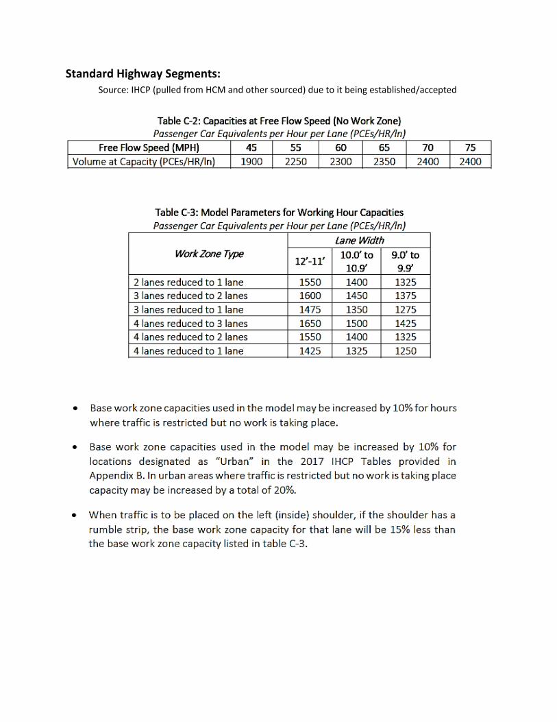
Standard Highway Segments: Source: IHCP (pulled from HCM and other sourced) due to it being established/accepted

Highway Ramps (Interstate to Interstate): Source: HCM Exhibit 13-10 Context: Limiting factor for most ramps will likely be the intersection, but C-Ds and Interstate to Interstate ramps are not limited in this way and can thus rely on this data

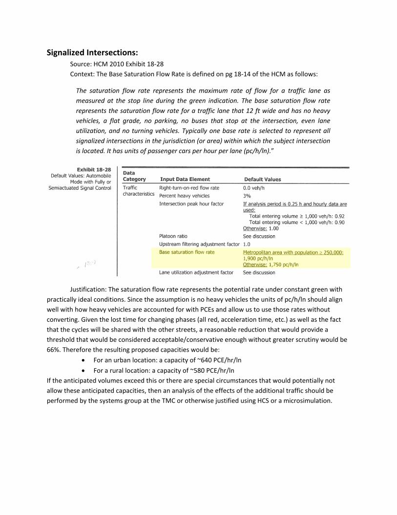
Signalized Intersections: Source: HCM 2010 Exhibit 18-28 Context: The Base Saturation Flow Rate is defined on pg 18-14 of the HCM as follows:

The saturation flow rate represents the maximum rate of flow for a traffic lane as measured at the stop line during the green indication. The base saturation flow rate represents the saturation flow rate for a traffic lane that 12 ft wide and has no heavy vehicles, a flat grade, no parking, no buses that stop at the intersection, even lane utilization, and no turning vehicles. Typically one base rate is selected to represent all signalized intersections in the jurisdiction (or area) within which the subject intersection is located. It has units of passenger cars per hour per lane (pc/h/ln).”

Justification: The saturation flow rate represents the potential rate under constant green with practically ideal conditions. Since the assumption is no heavy vehicles the units of pc/h/ln should align well with how heavy vehicles are accounted for with PCEs and allow us to use those rates without converting. Given the lost time for changing phases (all red, acceleration time, etc.) as well as the fact that the cycles will be shared with the other streets, a reasonable reduction that would provide a threshold that would be considered acceptable/conservative enough without greater scrutiny would be 66%. Therefore the resulting proposed capacities would be:

• For an urban location: a capacity of ~640 PCE/hr/ln • For a rural location: a capacity of ~580 PCE/hr/ln

If the anticipated volumes exceed this or there are special circumstances that would potentially not allow these anticipated capacities, then an analysis of the effects of the additional traffic should be performed by the systems group at the TMC or otherwise justified using HCS or a microsimulation.

Roundabouts: Source: NCHRP Report 672 (considered the current definitive reference for roundabouts) Link: http://onlinepubs.trb.org/onlinepubs/nchrp/nchrp_rpt_672.pdf Specific Page: 4-12, Exhibit 4-6 Comment: This doesn’t provide an exact value, but 600 PCE/hr seems reasonable unless the intersecting road is a very busy thoroughfare which leads to a lot of conflicting traffic opposing the ramp traffic. The analyst could reasonably go higher for locations with a high density of roundabouts (like Hamilton County) due to familiarity with RABs and willingness to accept smaller gaps.

TWSC Intersections: Source: HCM 2010 Chapter 19 Comment: The capacity of a TWSC intersection is the most difficult to estimate because the capacity of the minor road movements is so dependent on the traffic on the ‘major road’ (in this case, the road intersecting the interstate that the ramp traffic must stop for. To come up with something reasonable that could be applied in a more general case, the potential capacity (assuming there is no upstream signal affecting traffic at the interchange) was examined. Equation 19-32 offers a relatively

straightforward answer: 𝑐𝑐𝑝𝑝 = 𝑣𝑣𝑐𝑐 ∗𝑒𝑒−𝑣𝑣𝑐𝑐𝑡𝑡𝑐𝑐/3600

1−𝑒𝑒−𝑣𝑣𝑐𝑐𝑡𝑡𝑓𝑓/3600

where: 𝑐𝑐𝑝𝑝 is the potential capacity (vph) 𝑣𝑣𝑐𝑐 is the conflicting traffic volume (vph) 𝑡𝑡𝑐𝑐 is the critical headway for the minor movement (s) 𝑡𝑡𝑓𝑓 is the follow-up headway for the minor movement (s)

The default values for 𝑡𝑡𝑐𝑐 and 𝑡𝑡𝑓𝑓 used were 7.5 s (from Exhibit 19-10, LT from Minor Rd, 4 lanes on Major Rd, 1 stage movement with no median refuge) and 3.5 s (from Exhibit 19-11, LT from Minor Rd, 4 lanes on Major Rd), respectively. This should cover most locations at interchanges with this type of intersections and provide reasonably conservative results.

Based on the equation, the capacity for a range of major road volumes was calculated: The resulting capacities decrease from the theoretical maximum of 1027 vph (if there is virtually no cross-traffic on the major road) as the volume of traffic on the major road increases, which is expected. To check the validity/consistency of these results, HCS was used. The two sets of data for HCS 1 and HCS 2 had different distributions of traffic.

HCS 1 assumed parameters: • Single shared lane NB (minor road) • 2 lanes each on EB and WB with shared LT on EB and shared RT on WB • All minor road traffic was LT from NB • 50/50 split between directions on major road with all WB traffic going through and 20% of EB traffic turning left and 80% through. • Default values otherwise

HCS 2 assumed parameters:

• Single shared lane NB (minor road) • 2 lanes each on EB and WB with shared LT on EB and shared RT on WB • All minor road traffic was LT from NB • 50/50 split between directions on major road with all WB traffic going through and 50% of EB

traffic turning left and 50% through. • Default values otherwise

As shown in the table, the results for HCS 1 always yield capacities for the minor movement

greater than the base potential capacity. HCS 2 yields very similar results at lower volumes until it begins to deviate at about v = 700 vph. In this case the number of left turn vehicles from the major road allows less time for the minor road left turns. However, unless the interstate in the same direction as the exit ramp (in this case NB) is the destination, this is unlikely to be a factor and the calculated capacities should be sufficiently conservative.

vc (veh/h) cp (veh/h) HCS 1 HCS 2

1 1027 1029 1029

100 876 907 880

200 746 798 750

300 635 702 638

400 540 618 541

500 458 542 457

600 389 475 386

700 330 415 324

800 280 362 271

900 237 316 225

1000 200 275 186

1100 169 239 154

1200 143 207 126

1300 121 179 102

1400 102 155 82

1500 86 133 65

1600 72 115 51

1700 61 98 40

1800 51 84 30

1900 43 72 22

2000 36 61 15

AWSC Intersections: Source: HCM 2010 Chapter 20 Context: To simplify the possible variety of possible values I tried to distill the methodology to a representative intersection that would provide guidance on the capacity of an approach on a ramp (since we mainly want to make sure that queues don’t back-up to the interstate). To accomplish this I made the following assumptions and calculations:

1. To calculate roughly what the capacity would be for a single approach, I focused on the Saturation Headway. My understanding is that the saturation headway represents the minimum amount of time that would be required per vehicle to pass through the

intersection. Therefore: 1 𝑣𝑣𝑒𝑒ℎℎ

∗ 3600 𝑠𝑠𝑒𝑒𝑐𝑐ℎ𝑟𝑟

= 𝐶𝐶 where h is the saturation headway (eq 20-27 of

the 2010 HCM) and C is the capacity of a given approach. 2. Eq. 20-27 requires the base saturation headway and the saturation headway adjustment.

The adjustment requires knowledge of proportions of turning movements and heavy vehicles. I plan on accounting for this by rounding up to the nearest 0.5 seconds. The base saturation headway requires designations of groups and cases as shown in Exhibit 20-14. I will describe my determination of which case and group I selected below.

3. Exhibit 20-10 describes the Geometry Groups. Most ramps that will terminate at an AWSC intersection will likely have 2 lanes at most. Since the standard ramps I’m considering would be in a standard diamond configuration the result would be a 4-leg intersection with 0 lanes in the opposing approach. Most of these intersections will have no more than 2 lanes per approach for the conflicting approaches. This combination will result in the model intersection being in Geometry Group 5.

4. Similar to the reasoning in point 3, Exhibit 20-7 is the appropriate reference for the Degree-of-Conflict Case. With no opposing and both a conflicting left and right, the Case would 4.

5. Base to Exhibit 20-14, the max number of vehicles on the conflicting approaches would be 4.

Combined with Case 4 and Group 5, the resulting base saturation headway is 9.0 seconds.

6. To account for the headway adjustment given above, an additional 0.5 seconds is added,

resulting in a saturation headway of 9.5 seconds.

7. The resulting capacity would be 𝐶𝐶 = 1 𝑣𝑣𝑒𝑒ℎ9.5 𝑠𝑠𝑒𝑒𝑐𝑐

∗ 3600 𝑠𝑠𝑒𝑒𝑐𝑐ℎ𝑟𝑟

≅ 380 𝑣𝑣𝑣𝑣ℎ

8. For the purposes of analysis for an IHCP exception, the standard units are PCE/hr. The conversion of Veh/hr to PCE/hr is 1 for all smaller vehicles and 2 for all larger vehicles. Therefore, the capacity would be equal or greater once expressed as PCE/hr. Since we don’t have a constant proportion of trucks, the exact conversion is unknown, but using a capacity of 380 PCE/hr would be sufficiently conservative.