Embed Size (px)
Citation preview

Standard for Mapping Ecosystems at Risk in British Columbia
An Approach to Mapping Ecosystems at Risk and Other Sensitive Ecosystems
Prepared by Ministry of Environment
Ecosystems Branch for the
Resources Information Standards Committee
December 5, 2006
Version 1.0


© The Province of British Columbia Published by the Terrestrial Ecosystems Task Force Resources Information Standards Committee
Library and Archives of Canada Cataloguing in Publication Data Main entry under title:
Standard for mapping ecosystems at risk in British Columbia [electronic resource] : an approach to mapping ecosystems at risk and other sensitive ecosystems.
“December 5, 2006”—Cover. “Version 1.0”—Cover. Available on the Internet. Includes bibliographical references: p.
ISBN 978-0-7726-5699-5.
1. Environmental mapping – Standards - British Columbia. 2. Ecological mapping - Standards - British Columbia. 3. Vegetation mapping - Standards - British Columbia. 4. Endangered ecosystems – British Columbia. I. British Columbia. Resources Information Standards Committee. II. British Columbia. Ecosystems Branch.
QH541.15R57 S72 2007 333.95’220723 C2007-960043-3
Additional Copies of this publication can be purchased from:
Government Publication Services PO Box 9452 Stn Prov Govt 563 Superior Street 2nd Flr Victoria, BC V8W 9V7 Phone: (250) 387-6409 or Toll free: 1-800-663-6105 Fax: (250) 387-1120 http://www.publications.gov.bc.ca
Digital Copies are available on the Internet at: http://ilmbwww.gov.bc.ca/risc/.


Mapping Ecosystems at Risk
Abstract This report describes British Columbia standards for mapping ecosystems at risk including sensitive ecosystems. For the purposes of this document, ecosystems at risk are occurrences of ecological communities listed as special concern, threatened, or endangered by the British Columbia Conservation Data Centre (CDC) together with the abiotic and ecological processes at a particular site. Sensitive Ecosystems are those that are at-risk or are ecologically fragile in the provincial landscape. The information here has been developed for, and approved by, the Resources Inventory Standards Committee (RISC), a provincial committee responsible for developing provincial inventory standards.
These standards use two methods to map ecosystems at risk and other Sensitive Ecosystems: 1) using a Sensitive Ecosystems Inventory (SEI) method to map potential occurrences of ecosystems at risk and 2) modelling a Sensitive Ecosystems map from a Terrestrial Ecosystem Map (TEM), Predictive Ecosystem Map (PEM), or Broad Ecosystem Inventory (BEI).
The SEI mapping method is recommended where the primary goal of the project is to identify Sensitive Ecosystems, but funding is not sufficient for a TEM and there are no existing ecosystems maps for the study area. Sensitive Ecosystems categories are generalised groupings of ecosystems that share many characteristics, particularly ecological sensitivities, ecosystem processes, at-risk status, and wildlife habitat values. Sensitive Ecosystems categories used in SEI mapping projects vary according to region.
Similar to TEM, Sensitive Ecosystem units are delineated on aerial photographs or other imagery using vegetation, topographic, and terrain features. Ecosystem units are field verified, and site and vegetation attributes are recorded in a polygon database. The polygons are digitized and compiled in a geographic information system, and stored in a provincial database.
Where ecosystem mapping already exists, Sensitive Ecosystems can be modelled from an existing map. If no ecosystem mapping currently exists and funding is sufficient, a TEM with specific additional attributes, adjusted polygon delineation, and other considerations for Sensitive Ecosystems categories can be created and used to model a Sensitive Ecosystems map and database.
This report outlines the standards for Sensitive Ecosystem unit characterization, map symbols, field sampling, mapping procedures, legends, and reporting. It also outlines procedures for adapting TEM, PEM, and BEI to modelling Sensitive Ecosystems. Core data attributes collected for all Sensitive Ecosystems mapping projects in British Columbia are described, in addition to other attributes that are recommended to support conservation planning. Methods for mapping and evaluating ecological integrity of CDC element occurrences from Sensitive Ecosystems are described.
Sensitive Ecosystems maps provide a source from which to map element occurrences (EOs) of ecological communities at risk. Maps of EOs and other ecosystem maps inform some of the factors used by the CDC to evaluate the conservation status of an element. EOs of the highest ecological integrity can also be prioritized for practical conservation activities.
December 2006 i

Mapping Ecosystems at Risk
Acknowledgments The Government of British Columbia provides funding of the Resources Information Standards Committee work, including the preparation of this document. The Resources Information Standards Committee supports the effective, timely and integrated use of land and resource information for planning and decision making by developing and delivering focussed, cost-effective, common provincial standards and procedures for information collection, management and analysis. Representatives to the Committee and its Task Forces are drawn from the ministries and agencies of the Canadian and the British Columbia governments, including academic, industry and First Nations involvement.
The Resources Information Standards Committee evolved from the Resources Inventory Committee which received funding from the Canada-British Columbia Partnership Agreement of Forest Resource Development (FRDA II), the Corporate Resource Inventory Initiative (CRII) and by Forest Renewal BC (FRBC), and addressed concerns of the 1991 Forest Resources Commission.
For further information about the Resources Information Standards Committee, please access the RISC website at: http://ilmbwww.gov.bc.ca/risc/.
This report was developed by the B.C. Conservation Data Centre for the Terrestrial Ecosystems Task Force under the Resources Inventory Standards Committee (RISC). The B.C. Conservation Data Centre is a member of NatureServe, an international network of conservation organizations that provided the standards and methodology for status assessments and element occurrence ranking of ecosystems at risk.
Substantial contributions for this report have been provided by Carmen Cadrin and Jo-Anne Stacey of the BC Ministry of Environment and by Kristi Iverson, Iverson & MacKenzie Biological Consulting Ltd. Wherever possible, the report applies methods and digital data capture standards used in Terrestrial and Predictive Ecosystem mapping methods (Resources Inventory Committee 2000a, 2000b, 1999, and 1998b and Resources Inventory Standards Committee 2004a and 2004b). Keith Potter and the Soils Terrain Ecosystem Wildlife Inventory Data Committee (STEWI) provided invaluable assistance in data modeling and data management. Funding was provided for this project by the Forest Investment Account of British Columbia.
Environment Canada and the Canadian Wildlife Service, Ministry of Sustainable Resource Management and Ministry of Environment funded the development of the Sensitive Ecosystems Inventory standard through the Georgia Basin Action Plan.
Appreciation goes to reviewers Del Meidinger, Corey Erwin, Dave Clark, Jan Kirkby and Dan Bernier for their helpful comments and support in development of the standards, and Gina Varrin for technical support.
December 2006 ii

Mapping Ecosystems at Risk
Table of Contents Abstract .......................................................................................................................................i
Acknowledgments .................................................................................................................... ii
1 Introduction........................................................................................................................1
1.1 Rationale for Mapping Sensitive Ecosystems in British Columbia ...........................1
1.2 Hot Spots for Mapping Sensitive Ecosystems ...........................................................3
1.3 Ecosystem Classification and Mapping .....................................................................3
1.3.1 Sensitive and Other Important Ecosystems Classification.................................3
1.3.2 Ecosystem and Vegetation Classification in B.C...............................................4
1.3.3 CDC Ecological Communities at Risk...............................................................5
1.4 Choosing an Approach for Mapping Ecosystems at Risk and Sensitive Ecosystems6
1.5 Clients ........................................................................................................................7
2 Sensitive Ecosystems Inventory Mapping Method............................................................8
2.1 Introduction................................................................................................................8
2.2 Objectives ..................................................................................................................8
2.3 Planning the Inventory ...............................................................................................8
2.3.1 Survey Intensity .................................................................................................8
2.3.2 Map Scale.........................................................................................................11
2.3.3 Ecological assessment......................................................................................12
2.4 Development of the SEI Mapping Legend ..............................................................13
2.4.1 New SEI Units .................................................................................................13
2.4.2 Mapping Grassland and Related Ecosystems ..................................................13
2.5 Photo Interpretation .................................................................................................14
2.6 Field Sampling .........................................................................................................15
2.6.1 Designing a sampling plan...............................................................................16
December 2006 iii

Mapping Ecosystems at Risk
2.6.2 Conducting field inspections and plot sampling.............................................. 17
2.6.3 Field Data Capture, Synthesis, and Analysis................................................... 18
2.7 Non-spatial Attribute Data ...................................................................................... 19
2.7.1 Project Attributes............................................................................................. 19
2.7.2 Core Polygon Attributes .................................................................................. 19
2.7.3 Optional and Recommended Polygon Attributes ............................................ 20
2.7.4 User-Defined Attributes .................................................................................. 20
2.8 Spatial Digital Data Capture.................................................................................... 21
2.9 Biogeoclimatic (BGC) and Ecosection Linework ................................................... 21
2.10 Accuracy Assessment and Quality Assurance......................................................... 21
2.11 Reporting ................................................................................................................. 21
2.12 Digital Data Deliverables ........................................................................................ 23
2.12.1 Spatial Data ..................................................................................................... 24
2.12.2 Non-Spatial Data Deliverables ........................................................................ 24
2.13 Map Production ....................................................................................................... 25
2.13.1 Polygon Labels ................................................................................................ 25
2.13.2 Map Linework ................................................................................................. 26
2.13.3 Map Legend and Map Surround...................................................................... 26
3 Modelling SEI ................................................................................................................. 28
3.1 Terrestrial Ecosystem Mapping............................................................................... 28
3.1.1 Bioterrain mapping.......................................................................................... 28
3.1.2 Sampling strategy ............................................................................................ 28
3.1.3 New ecosystem classification.......................................................................... 29
3.1.4 Additional Attributes ....................................................................................... 29
3.1.5 Developing the SEI Theme.............................................................................. 30
3.1.6 Digital Data Deliverables ................................................................................ 32
December 2006 iv

Mapping Ecosystems at Risk
3.1.7 Map Production................................................................................................33
3.2 Predictive Ecosystem Mapping................................................................................33
3.2.1 Modelling SEI maps from PEM.......................................................................34
3.2.2 Using PEM Directly to Map Sensitive Ecosystems.........................................34
3.2.3 Digital Data Deliverables.................................................................................35
3.2.4 Map Production................................................................................................36
3.3 Broad Ecosystem Mapping ......................................................................................36
3.4 Limitations on Using Pre-existing Map Products ....................................................37
3.5 Accuracy Assessments.............................................................................................37
4 CDC Methods ..................................................................................................................38
4.1 Element Conservation Status Assessments..............................................................38
4.2 Element Occurrence Ranking ..................................................................................39
4.3 Ecological Community Landscape Types................................................................40
4.4 Element Occurrence Specifications .........................................................................40
4.4.1 Separating Element Occurrences .....................................................................41
4.4.2 Element Occurrence Rank Criteria ..................................................................42
4.5 Element Occurrence Ranking Procedure .................................................................45
4.6 Examples of Element Occurrences and Ranking .....................................................47
4.6.1 Riparian EO Ranking Example 1.....................................................................47
4.6.2 Riparian EO Ranking Example 2.....................................................................48
5 Mining Ecosystem Maps for Element Occurrences of Ecological Communities at Risk50
References................................................................................................................................54
Appendix A: Glossary..............................................................................................................58
Appendix B: Conservation Evaluation Form...........................................................................61
Appendix C: United States National Vegetation Classification System..................................63
Appendix D: SEI Map Codes, Map Units and Descriptions....................................................64
December 2006 v

Mapping Ecosystems at Risk
Appendix E: Data Dictionary .................................................................................................. 71
Appendix F: Example Vegetation Tables for SEI Reports...................................................... 79
Appendix G: Example SEI Ratings Table............................................................................... 80
Appendix H: Example Element Occurrence Specifications.................................................... 81
Matrix South Coast Circumesic Forests Example Element Occurrence Specification ....... 81
Matrix Grassland Element Occurrence Specification.......................................................... 83
Appendix I: Example Separation Distance Specifications ...................................................... 87
Example Separation Distances for Matrix Communities .................................................... 87
Example Separation Distances for Large Patch Communities ............................................ 87
Example Separation Distances for Small Patch Communities ............................................ 87
Example Separation Distances for Linear Communities..................................................... 88
December 2006 vi

Mapping Ecosystems at Risk
1 Introduction This report presents the range of methods available to map ecosystems at risk, other Sensitive Ecosystems and Other Important Ecosystems around the province. A Sensitive Ecosystem is one that is at-risk or ecologically fragile in the provincial landscape. Ecosystems at risk are those that can support ecological communities which are considered to be provincially at risk as designated by the B.C. Conservation Data Center (CDC; http://www.env.gov.bc.ca/cdc/) and are listed as either ‘Red’ (extirpated, endangered, or threatened) or ‘Blue’ (special concern). However, other ecosystems at risk also exist that have not yet been described or listed, but which can be mapped within a Sensitive Ecosystem unit. Other Important Ecosystems have significant ecological and biological values associated with them that can be identified and mapped, although they are not defined as Sensitive Ecosystems.
This report provides standards for data capture relating specifically to ecosystems at risk and other Sensitive Ecosystems. The methods provided here are based on existing ecosystem mapping methods (Resources Inventory Committee 1998a, 1998b, 1999, 2000a, and 2000b; Resources Inventory Standards Committee 2004a and 2004b, Iverson and Cadrin 2003, McPhee et al. 2000, Ward et al. 1998). This report also documents the CDC inventory, mapping and conservation evaluation methods (NatureServe 2002) and provides methods for mapping verified occurrences of ecological communities at risk (called “element occurrences”) from Sensitive Ecosystems and other ecosystem maps. Occurrences with the highest ecological integrity (see viability for species) (NatureServe 2002) can be prioritized for conservation measures.
Current sources of information for ecological communities at risk in BC consist of the CDC database, Ecological Reserves Program documents, B.C. Ministry of Forests’ biogeoclimatic ecosystem classification system, wildlife and wildlife habitat inventory projects, ecosystem mapping projects (including historical mapping of ecosystems), published and unpublished reports, various theses, and other papers from a variety of sources. This information forms the basis of conservation status assessments of known ecological communities in the province. The CDC compiles this information, using a standardized system of information storage and retrieval common to a wide network of similar programs from Latin America, U.S.A. and Canada (see http://www.natureserve.org).
1.1 Rationale for Mapping Sensitive Ecosystems in British Columbia
There is an emerging recognition that healthy ecosystems provide the foundation that sustains all life (Ward and Dawe 2001) and conservation of the Province’s biological diversity is a priority for British Columbians. To make biologically sustainable decisions we first need to know what our biological resources are, where they occur, and, if possible, where they used to occur. Inventory and mapping of the Province’s ecological systems at a variety of scales provides the vital link, informing land use planning and decision making to protect critical elements of biodiversity.
Currently, there are a number of ecosystems in B.C. that are on the verge of extirpation or extinction such as antelope-brush ecosystems and Garry oak ecosystems. These and other threatened ecosystems and ecosystems of special concern are referred to as ‘ecological
December 2006 1

Mapping Ecosystems at Risk
communities at risk’ by the CDC. Additionally, there are other ecosystems that are ecologically sensitive to disruption by human-caused effects1. Sensitive Ecosystems include both ecological communities at risk and ecosystems that are ecologically sensitive. Sensitive Ecosystems provide habitat for many species, including many plants and animals at risk; they perform functions that influence their environment such as filtering water and reducing carbon dioxide levels, and they set the stage for the complex interactions between organisms. Losing these ecosystems can negatively impact the species that depend on them, including critical habitat for species at risk. Loss and degradation of ecosystems could have far reaching effects on local ecological health that we cannot yet fully understand.
Ensuring that examples of every ecosystem are maintained in a natural state supports sustainable resource management. These natural ecosystems serve as “benchmarks” against which our success in managing our natural resources can be measured, and serve as reference points for restoring ecosystems that have been altered or destroyed. Mapping Sensitive Ecosystems can help inform land management decisions, provide direction for more detailed inventories, and help set management and conservation priorities. By protecting natural ecosystems, we may enjoy and benefit from them in the future, as we have in the past.
The first Sensitive Ecosystems Inventory (SEI) was developed by the CDC and Environment Canada, Canadian Wildlife Service (CWS). Sensitive Ecosystems Inventory: East Vancouver Island and the Gulf Islands (Ward et al. 1998) was initiated in 1994 and completed in 1997.
SEI mapping allows for the inclusion of previously undocumented ecological communities and unique ecosystems2 through the use of physiognomic classification and broad vegetation categories. Sensitive Ecosystem classes are used because ecosystem description at a general level is usually more appropriate for local planning and public education.
In 2003, CWS conducted an evaluation to determine the success of using SEIs in conserving sensitive and Other Important Ecosystems (Axys Environmental Consulting Ltd. 2003). Based on a review of aerial photographs from 2002, it was found that nearly 4.6% of the seven Sensitive Ecosystems3 had been lost since the late 1990s (losses were 11% when the two Other Important Ecosystem types4 are included). These figures are especially significant considering that less than 8% of the landscape was mapped as Sensitive Ecosystems in the original SEI. Although the SEI mapping did not prevent further loss of Sensitive
1 Ecological sensitivities are processes or components of ecosystems that are susceptible to disruption or damage by an external factor. For example, changes to the hydrological regime of wetlands and riparian areas can alter the species composition and the ecological functions of the system. Ecosystems with very shallow soils are sensitive because they are particularly susceptible to overuse, soil loss, degradation and colonization or spread of invasive alien plants. 2 Unique ecosystems are ecosystems that occur too infrequently on the landscape to be included in other provincial classification systems. 3 For the SEI for East Vancouver Island and Gulf Islands, the seven sensitive ecosystems were coastal bluff, terrestrial herbaceous, older forest, riparian, sparsely vegetated, woodland, and wetland. 4 The two other ecosystem types included in the SEI for East Vancouver Island and Gulf Islands were seasonally flooded agricultural fields and older second growth forests. These ecosystem types, although altered by human use and therefore not considered at-risk and sensitive, were included for their overall biodiversity and wildlife habitat values.
December 2006 2

Mapping Ecosystems at Risk
Ecosystems, users of the SEI mapping indicated that the SEI had contributed to the conservation of numerous sites between 1997 and 2002.
Axys Environmental Consulting Ltd. (2003) found that over those five years the SEI was used in a variety of land use planning processes. Ninety-six percent of decision makers used the SEI when considering land development, capital works, site enhancement, and mitigation. All Regional Districts in the study area had incorporated the SEI into Official Community Plans and three of four used the SEI for Development Permit Area designation.
Users of SEI mapping included local government (municipal and regional) for park planning as well as specifics mentioned above. The provincial government has used SEI mapping in identifying areas for Old Growth Management Designation (Reynolds 2000) and forest companies have either initiated their own SEI mapping for planning processes or supported and applied SEI mapping in operational planning (Beese and Fujikawa 2003; Marquis 2002). Local natural history groups, land trusts, and conservation groups have used SEI mapping to raise the profile of conservation priority sites and to influence conservation-based land use decisions.
Sensitive Ecosystems Inventory mapping projects have been completed, or are in process, for the Georgia Basin and the Okanagan Valley, two areas in British Columbia with the highest number of species and ecosystems at risk in B.C (see http://www.env.gov.bc.ca/sei/)..
1.2 Hot Spots for Mapping Sensitive Ecosystems The highest concentrations of Sensitive Ecosystems lie within specific geographic areas of the province or are associated with specific landscape features. Southeast Vancouver Island and Gulf Islands, the lower mainland, major southern interior valleys, and the southern Rocky Mountain Trench are some of the areas which contain the most Sensitive Ecosystems. Ecosystems within landscape features such as valley bottoms, lower slopes, and floodplains are threatened throughout the province. Grassland landscapes are particularly vulnerable to the introduction and spread of invasive alien species. Areas expressing major physiographic changes, with high concentrations of varying physical features, fault lines and areas of atypical geologic types, major climatic transition zones, uncommon geomorphological processes, regions of natural endemism, and glacial refugia are all places where unusual natural ecosystems are expected to occur and which should be the subject of intensive field inventory.
1.3 Ecosystem Classification and Mapping The Sensitive Ecosystems classification, Ministry of Forests’ ecosystem classification system, and the classification system used by the CDC are described below. This report uses the term “ecosystem at risk” to refer to the at-risk ecological community together with the abiotic and ecological processes at a particular site. The terms ‘ecological community’, ‘plant community’, ‘plant association’, ‘ecosystem’, and ‘ecosystem at risk’ are also defined.
1.3.1 Sensitive and Other Important Ecosystems Classification The classification system used in the Sensitive Ecosystems Inventories (SEI) broadly follows the categories applied in NatureServe’s ecological systems classification (Anderson et al.
December 2006 3

Mapping Ecosystems at Risk
1998). Sensitive Ecosystem classes are also partly based on the formation class level of the United States National Vegetation Classification System (Grossman et al. 1998) and the physiognomic classification system of the United Nations Educational, Scientific and Cultural Organization (1973).
The SEI classification uses two primary groupings of ecosystems: Sensitive Ecosystems and Other Important Ecosystems. Within each of these groups a series of classes and subclasses is defined that provides a general level of ecosystem description that is appropriate for public education and local planning exercises. Sensitive Ecosystem categories are generalised groupings of ecosystems that share many characteristics, particularly ecological sensitivities, ecosystem processes, at-risk status, and wildlife habitat values. Criteria for ecological sensitivity include: environmental specificity, susceptibility to hydrological changes, soil erosion, especially on shallow soils, spread of invasive alien plants, and sensitivity to human disturbance. Other Important Ecosystems5 have significant ecological and biological values associated with them that can be identified and mapped, although they are not defined as Sensitive Ecosystems because they have been substantially altered by human use. Consideration of Other Important Ecosystems is critical to capturing key elements of biodiversity of some project areas; they sometimes provide recruitment sites for ecosystems at risk or important wildlife habitat requiring recovery or restoration.
Currently accepted Sensitive and Other Important Ecosystem classes and subclasses are listed in Appendix D: SEI Map Codes, Map Units and Descriptions.
1.3.2 Ecosystem and Vegetation Classification in B.C. The B.C. Ministry of Forests’ biogeoclimatic ecosystem classification (BEC) system integrates climate, soil, and vegetation data into a single ecological classification system. The province has been divided up into biogeoclimatic units, or areas with relatively similar regional climates, inferred from late successional vegetation on zonal sites6. Biogeoclimatic units include zones, subzones, variants and phases. BEC has focussed on classifying late successional plant associations, often using sample plot data from mature seral or climax vegetation. (Pojar et al. 1991)
The plant association is the basic vegetation unit of BEC. Plant associations are formally recognized units that are differentiated using diagnostic combinations of plant species and are based on a number of stands of late successional vegetation that have very similar species and structure.
The first definition of a plant association to appear in published literature was “a plant community type of definite floristic composition, uniform habitat conditions, and uniform physiognomy.” (Flahault and Schroter 1910). The currently accepted definition is: “A
5 Examples:
1) Seasonally flooded fields are often converted wetlands which continue to provide critical wildlife habitat at certain times in the year for certain migratory species, and 2) Disturbed grasslands that have a significant component of alien plants still provide habitat for many red- and blue-listed species.
6 Zonal ecosystems are those which best reflect the regional climate of the area and are not influenced by local relief, or by any properties of parent materials.
December 2006 4

Mapping Ecosystems at Risk
vegetation classification unit defined on the basis of a characteristic range of species composition, diagnostic species occurrence, habitat conditions and physiognomy.” (Vegetation Classification Panel, Ecological Society of America 2004). The Ministry of Forests’ BEC definition of a plant association is similar and uses similar concepts.
Plant associations in BEC are named after one to four plant species that dominate or characterize the unit (e.g., Pseudotsuga menziesii – Juniper communis – Penstemon). There is always some variation within a plant association, but all stands within a plant association have features in common that distinguish them from other plant associations. The vegetation species composition and structure must fall within the expected range of the defined plant association before it is considered an occurrence of that particular plant association.
Vegetation changes over time through succession, usually in response to a disturbance such as fire or logging. A particular stand of vegetation can progress from one plant association to another over time. Each successional stage of vegetation, from recent clear-cuts to old-growth forests, can often be classified as a separate plant association.
BEC includes a site classification system where the basic unit is the site association, sites that have the same environmental properties and potential to develop similar climax vegetation, regardless of present vegetation. Site associations are all ecosystems capable of producing the same plant association in a climax ecosystem. They are identified by the environmental properties that control vegetation.
Site associations are further differentiated as site series within the subzone or variant. Because a subzone has a relatively uniform climate, site series are usually more uniform in nature than the site association or plant association. Site series identify the abiotic attributes of an ecosystem and indicate that the late successional plant association may occur there, or has the potential to occur there through time.
Site series are usually given the same name as the site association they belong to, together with the biogeoclimatic subzone, variant or phase (e.g., IDFxm/Douglas-fir – Bluebunch wheatgrass – Penstemon). They are also given a numeric code (e.g., IDFxm/02). Field guides for identifying site series have been prepared for each forest region in the province. Site series are the units mapped in terrestrial ecosystem maps (TEM) and the unit that B.C. ecologists are most familiar with.
The BEC framework was primarily designed to meet the needs of forest and range managers. Recently, the classification of wetland and grassland site associations has been significantly expanded. Classification of alpine and parkland ecosystems is underway. Classification of smaller or extremely localized ecosystems, such as vernal pools and coastal sand dunes has not been funded under the BEC system.
1.3.3 CDC Ecological Communities at Risk Ecological communities at risk are those identified by the B.C. CDC as special concern, threatened or endangered. The CDC has adopted the plant associations from the vegetation component of BEC as the primary source for terrestrial ecological communities. The CDC uses information from mapping projects, reports, and local expertise to identify and list other ecological communities not included in the BEC vegetation classification. The term ecological community was chosen to allow the inclusion of non-terrestrial communities including aquatic and marine communities.
December 2006 5

Mapping Ecosystems at Risk
Although the terms “ecological community”, “ecosystem” and “plant community” or “plant association” are often used interchangeably, they are not equivalent. “Plant community” refers to the assemblage of vegetation on a site. “Plant association” is a formal term applied by a rigorous classification process. Mueller-Dombois and Ellenberg (1974) suggest “association” be used only in the abstract sense and “community” is best used for a concrete example in the field. “Ecosystem” refers to the abiotic, biotic (e.g., plant and animal community), and ecological processes on a site. The term “ecosystem at risk” refers to a specific site and the ecological community at risk that grows on it. We generally map ecosystems based on vegetation structure, disturbance, soil and terrain characteristics, and other information about the specific site, especially field verified data.
Ecological communities tend to be broader ecological units than site series; one ecological community can include the potential vegetation on more than one site series. The site series is the “habitat” for the particular ecological community. Habitat for ecological communities is defined by Grossman et al. (1998) as “the combination of environmental (site) conditions and ecological processes (such as disturbances) influencing the community.” Thus, the CDC does not list specific site series as “at-risk”, however, since site series are more widely recognized and used in resource management in British Columbia, the CDC cross references site series with the potential to develop certain ecological communities.
Workers in the field can use their skills in identifying site series to locate at-risk ecological communities. Earlier successional stages can be important recruitment sites for future occurrences of ecological communities at risk. Thus, it is important to identify and distinguish between present occurrences of ecological communities at risk and sites (or site series) with the potential to develop an ecological community at risk in the future (Section 5).
1.4 Choosing an Approach for Mapping Ecosystems at Risk and Sensitive Ecosystems
There are several options for mapping ecosystems at risk and Sensitive Ecosystems depending on inventory goals, information needs, existing information or mapping, and cost.
The primary method, Sensitive Ecosystems Inventory (SEI) mapping, is recommended where the primary goal of the project is to locate at-risk or Sensitive Ecosystems, but funding is not sufficient for Terrestrial Ecosystem Mapping (TEM) and no ecosystem maps exist for the study area.
If the project has additional planning goals such as wildlife habitat mapping or terrain stability mapping, SEI mapping modelled from new TEM mapping is recommended.
Where ecosystem mapping already exists, including TEM, Predictive Ecosystem Mapping (PEM), or Broad Ecosystem Inventory mapping (BEI), it may be useful to model a Sensitive Ecosystems map from this existing map (see Section 3). A themed map can indicate if upgrades are required to the existing map product or if a new map product is required. Limitations to using existing map products are described in Section 3.4.
TEM provides detailed ecosystem information that is suitable for a number of additional mapping interpretations including wildlife habitat mapping. A key feature of TEM, with
December 2006 6

Mapping Ecosystems at Risk
respect to mapping ecosystems at risk, is that the entire study area is mapped7 and up to three ecosystems are mapped in each polygon. These features enable TEM to be used to determine vegetation structure and the viability of ecosystems at risk by providing details of the site and surrounding landscape.
PEM provides similar information to TEM, but has less detailed information for each polygon. Most PEM products indicate the probability of one ecosystem occurring within each polygon. Occasionally PEM products indicate the percentage of different ecosystems in a polygon, similar to TEM. Although PEM can be used to map some ecosystems at risk, it often has limited abilities to capture areas of unique environmental specificity, and to distinguish between ecosystems that occupy sites with similar physical attributes (e.g., circumesic sites). PEM products will vary in their usefulness for modelling Sensitive Ecosystems depending on the original information sources used and the objectives of the project.
BEI is a small scale (1:250 000), provincial coverage that is generally only appropriate for strategic landscape level analysis to identify general areas with high potential for occurrences of ecosystems at risk.
1.5 Clients Clients in different sectors are likely to have different objectives and needs with respect to mapping ecosystems at risk. These objectives can be used to guide initial decision-making in choosing an appropriate mapping method.
Forestry clients with specific needs related to certification, forest productivity, silviculture, and wildlife habitat planning can use TEM to achieve landscape-level objectives and some operational objectives.
Provincial and federal parks and protected area managers are likely concerned with both conservation (including element occurrences of ecological communities at risk) and recreation (BC Ministry of Environment, Lands and Parks 1998). These clients may have additional needs such as wildlife habitat mapping that are best met by using a TEM base for the ecosystems at risk map.
Local Governments including Municipalities and Regional Districts may choose either an SEI or TEM approach. SEI is the best approach where the only focus is on Sensitive Ecosystems. TEM is the best approach when planning for the whole landscape or where other considerations such as wildlife habitat mapping are of interest in the study area.
7 In TEM, all known ecosystems that can be distinguished at the mapping scale are mapped. However, it is likely that there are smaller, not yet described, and possibly at-risk ecosystems that may not be mapped.
December 2006 7

Mapping Ecosystems at Risk
2 Sensitive Ecosystems Inventory Mapping Method
2.1 Introduction Sensitive Ecosystems Inventory (SEI) mapping was developed in 1993 by the B.C. CDC and Environment Canada’s Canadian Wildlife Service in response to a need for inventory of at-risk and ecologically fragile ecosystems, and critical wildlife habitat areas on the east side of Vancouver Island.
The SEI mapping initiative predated the Resources Inventory Committee (RIC) standard for Terrestrial Ecosystem Mapping (TEM) and pioneered an approach that would flag sites for more detailed inventory prior to making land use decisions and to facilitate landscape level planning. The intent of the SEI mapping was to provide a less intensive and expensive mapping method. The first Sensitive Ecosystems Inventory project was completed in 1997 (Ward et al. 1998).
This document provides detailed methods and RISC standards to complete SEI mapping; the methods and standards are based on both the original SEI methods and more recent RIC and Resources Inventory Standards Committee (RISC) standards for TEM and PEM. Appendix D: SEI Map Codes, Map Units and Descriptions, provides a list of provincially accepted SEI classes and subclasses for Sensitive and Other Important Ecosystems.
2.2 Objectives The primary objective of SEI mapping is to provide information for the conservation of ecological diversity, particularly the most vulnerable and rare elements in the landscape. The use of this standard will promote consistency in results of SEI mapping throughout the province. The level of inventory can vary based on client needs but ecosystems at risk are most commonly mapped at 1:20 000 with survey intensity level 3 (see Table 1). Many clients may have multiple objectives and mapping should be tailored to objectives with the most specific needs.
2.3 Planning the Inventory Successful inventories begin with careful planning and consideration of the client’s needs. This provides the basis for determining the project objectives and required approach and products. A review of all previous inventories of the area can assist in selecting the appropriate and most cost effective inventory method. Once the objectives and products are determined, the survey intensity level and mapping scale is established (see Table 1).
2.3.1 Survey Intensity Table 1 compares project objectives to various survey levels and map scales. Survey level indicates the proportion of polygons that are field inspected and the ratio of different plot types used in field inspections (Resources Inventory Committee 2000a). Higher levels of
December 2006 8

Mapping Ecosystems at Risk
December 2006 9
survey intensities should provide higher levels of map reliability, but will cost more. Survey intensities should be tailored to meet client-specific needs for map reliability. The acceptable level of map reliability is directly linked to the intended uses of the mapping. Field inspections can be focused on certain portions of the landscape (e.g., ecosystems at risk and other Sensitive Ecosystems) to provide a higher level of reliability for that portion of the landscape.

Mapping Ecosystem
s at Risk
10
Decem
ber 2006
Survey Intensity
Level
Percentage of Polygon Inspections
Ratio of Full Plots:
Ground Insp.: Visual Checks1
Suggested Scales
(K =1000)
Area Covered by
0.5 cm2
Range of Study Area (ha) Example Project Objectives
1 76–100% 2 : 98 : 0 1:1 K to 1:10 K
0.0025–0.5 ha
0.025–100 Restoration planning, conservation covenants and conservation tax credits, element occurrence mapping. Site specific environmental impact assessments for energy, housing, or other developments. May be used to refine larger scale mapping for sites of specific interest.
2 51–75% 6 : 24 : 70 1:10 K to 1:20 K
0.5–2 ha 50–5 000 Local government land use planning (zoning, OCP, DPs, and growth strategies), greenways and park planning, element occurrence mapping, medium scale pre-planning for energy, housing, or other developments (e.g., neighbourhood plan or rezoning).
3 26–50% 6 : 24 : 70 1:10 K to 1:50 K
0.5–12.5 ha 1 000– 50 000 Landscape level land use planning, land acquisition priorities, habitat mapping and habitat protection, element occurrence mapping.
4 15 – 25% 5 : 20 : 75 1:20 K to 1:50 K
2–12.5 ha 10 000–500 000 Land use planning, conservation priorities, SOE reporting.
R 0–14% 0 : 25 : 75 1:100 K to 1:250 K
25–156 ha 50 000–1 000 000+ Strategic level land use planning for forest companies or local governments, SOE reporting.
Table 1 - Survey Intensity Levels and Map Scales (adapted from Resources Inventory Committee 1998b).
1 Inspection ratios are guidelines; actual project ratio should be set by the project ecologist.
Mapping Ecosystems at Risk
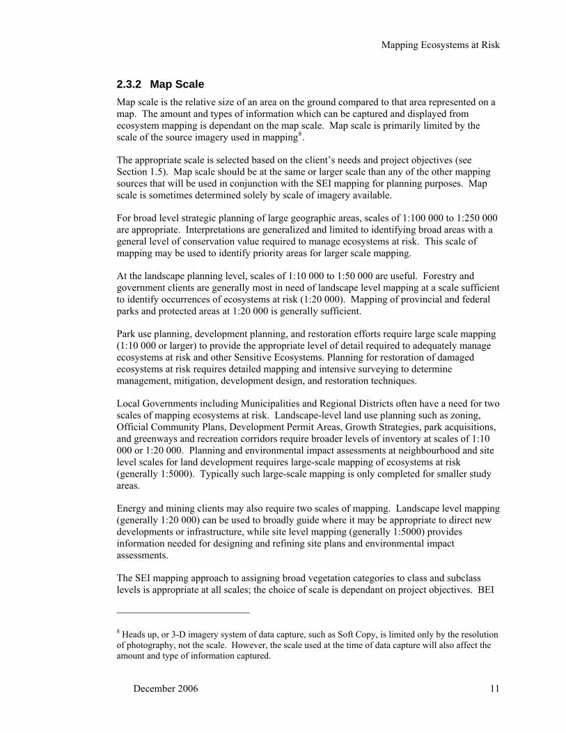
2.3.2 Map Scale Map scale is the relative size of an area on the ground compared to that area represented on a map. The amount and types of information which can be captured and displayed from ecosystem mapping is dependant on the map scale. Map scale is primarily limited by the scale of the source imagery used in mapping8.
The appropriate scale is selected based on the client’s needs and project objectives (see Section 1.5). Map scale should be at the same or larger scale than any of the other mapping sources that will be used in conjunction with the SEI mapping for planning purposes. Map scale is sometimes determined solely by scale of imagery available.
For broad level strategic planning of large geographic areas, scales of 1:100 000 to 1:250 000 are appropriate. Interpretations are generalized and limited to identifying broad areas with a general level of conservation value required to manage ecosystems at risk. This scale of mapping may be used to identify priority areas for larger scale mapping.
At the landscape planning level, scales of 1:10 000 to 1:50 000 are useful. Forestry and government clients are generally most in need of landscape level mapping at a scale sufficient to identify occurrences of ecosystems at risk (1:20 000). Mapping of provincial and federal parks and protected areas at 1:20 000 is generally sufficient.
Park use planning, development planning, and restoration efforts require large scale mapping (1:10 000 or larger) to provide the appropriate level of detail required to adequately manage ecosystems at risk and other Sensitive Ecosystems. Planning for restoration of damaged ecosystems at risk requires detailed mapping and intensive surveying to determine management, mitigation, development design, and restoration techniques.
Local Governments including Municipalities and Regional Districts often have a need for two scales of mapping ecosystems at risk. Landscape-level land use planning such as zoning, Official Community Plans, Development Permit Areas, Growth Strategies, park acquisitions, and greenways and recreation corridors require broader levels of inventory at scales of 1:10 000 or 1:20 000. Planning and environmental impact assessments at neighbourhood and site level scales for land development requires large-scale mapping of ecosystems at risk (generally 1:5000). Typically such large-scale mapping is only completed for smaller study areas.
Energy and mining clients may also require two scales of mapping. Landscape level mapping (generally 1:20 000) can be used to broadly guide where it may be appropriate to direct new developments or infrastructure, while site level mapping (generally 1:5000) provides information needed for designing and refining site plans and environmental impact assessments.
The SEI mapping approach to assigning broad vegetation categories to class and subclass levels is appropriate at all scales; the choice of scale is dependant on project objectives. BEI
8 Heads up, or 3-D imagery system of data capture, such as Soft Copy, is limited only by the resolution of photography, not the scale. However, the scale used at the time of data capture will also affect the amount and type of information captured.
December 2006 11

Mapping Ecosystems at Risk
is appropriate for 1:100 000 to 1:250 000 scale projects. PEM is appropriate for larger scales, generally to a limit of 1:20 000 (or larger, if mapping products used in the modelling are at a larger scale). Most PEM projects are completed at a scale of 1:20 000 because of the scale of input data sources. TEM is appropriate for all scales larger than, and including 1:50 000. The scale of TEM should be primarily determined by project objects, but practically, the availability of imagery and funding may limit the scale of the project.
2.3.3 Ecological assessment The first step towards developing an SEI map is to assess which ecologically Sensitive Ecosystems are likely to occur in the landscape. This would include determining which red- and blue-listed ecological communities are expected to occur within the study area and other elements of the landscape and vegetation that are unique or sensitive. Ecologically Sensitive Ecosystems that are not yet considered at-risk, as well as ecosystems restricted to very specific environmental conditions, must be considered for inclusion in a Sensitive Ecosystems class. The potential discovery of previously undocumented or unique ecosystem types is built into the inventory through an analysis of landscape features listed in Table 2 which are then incorporated into the field sampling plan. Potential information sources include bedrock geology maps, soils maps, biogeoclimatic maps, topographic maps, and information from local ecologists and naturalists.
Table 2 - Areas of atypical environmental characteristics (from Maxwell et al. 1993). 1. Physiographic Anomaly
• Areas where varied Ecosections meet; areas that express a major change in physiography. • Areas with high concentration of varying physical features. • Areas of converging major valley systems, creating complex climate mixes.
2. Geologic Anomaly • Areas of bedrock types that create atypical soil chemistry • Areas with major fault lines.
3. Climatic Anomaly • Areas where varied biogeoclimatic subzones meet; areas with major changes in climate • Areas associated with landscape features that modify local climates
4. Surficial Process Anomalies • Areas with uncommon landform features created by surficial processes of erosion and
deposition (e.g., sand dunes, eskers, cliffs, canyons, kettle and kame, hoodoos, karst) 5. Vegetation Anomalies (small scale)
• Disjunction: areas with dominant vegetation disjunct from its normal distribution • Areas with recorded at-risk plant locations • Endemism: natural areas where there is a high degree of endemic populations • Remnant vegetation type now depleted and fragmented by human development or actions • Glacial refugia
6. Moisture Regime Anomalies • In a dry climate, areas associated with water • In a wet climate, dry areas
7. Water Anomalies • Areas containing water bodies with unusual temperature or chemistry characteristics
12 December 2006
Mapping Ecosystems at Risk
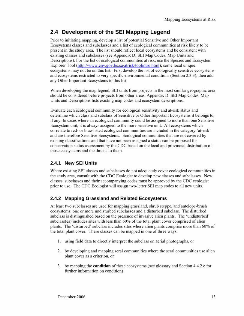
2.4 Development of the SEI Mapping Legend Prior to initiating mapping, develop a list of potential Sensitive and Other Important Ecosystems classes and subclasses and a list of ecological communities at risk likely to be present in the study area. The list should reflect local ecosystems and be consistent with existing classes and subclasses (see Appendix D: SEI Map Codes, Map Units and Descriptions). For the list of ecological communities at risk, use the Species and Ecosystem Explorer Tool (http://www.env.gov.bc.ca/atrisk/toolintro.html); some local unique ecosystems may not be on this list. First develop the list of ecologically sensitive ecosystems and ecosystems restricted to very specific environmental conditions (Section 2.3.3), then add any Other Important Ecosystems to this list.
When developing the map legend, SEI units from projects in the most similar geographic area should be considered before projects from other areas. Appendix D: SEI Map Codes, Map Units and Descriptions lists existing map codes and ecosystem descriptions.
Evaluate each ecological community for ecological sensitivity and at-risk status and determine which class and subclass of Sensitive or Other Important Ecosystems it belongs to, if any. In cases where an ecological community could be assigned to more than one Sensitive Ecosystem unit, it is always assigned to the more sensitive unit. All ecosystems which correlate to red- or blue-listed ecological communities are included in the category ‘at-risk’ and are therefore Sensitive Ecosystems. Ecological communities that are not covered by existing classifications and that have not been assigned a status can be proposed for conservation status assessment by the CDC based on the local and provincial distribution of those ecosystems and the threats to them.
2.4.1 New SEI Units Where existing SEI classes and subclasses do not adequately cover ecological communities in the study area, consult with the CDC Ecologist to develop new classes and subclasses. New classes, subclasses and their accompanying codes must be approved by the CDC ecologist prior to use. The CDC Ecologist will assign two-letter SEI map codes to all new units.
2.4.2 Mapping Grassland and Related Ecosystems At least two subclasses are used for mapping grassland, shrub steppe, and antelope-brush ecosystems: one or more undisturbed subclasses and a disturbed subclass. The disturbed subclass is distinguished based on the presence of invasive alien plants. The ‘undisturbed’ subclass(es) includes sites with less than 60% of the total plant cover comprised of alien plants. The ‘disturbed’ subclass includes sites where alien plants comprise more than 60% of the total plant cover. These classes can be mapped in one of three ways:
1. using field data to directly interpret the subclass on aerial photographs, or
2. by developing and mapping seral communities where the seral communities use alien plant cover as a criterion, or
3. by mapping the condition of these ecosystems (see glossary and Section 4.4.2.c for further information on condition)
December 2006 13

Mapping Ecosystems at Risk
When mapping condition, ‘excellent’ (<5% alien non-invasive species), ‘good’ (5-20% alien species), and ‘fair’ (21-60 % alien species) correspond to the undisturbed subclass(es); ‘poor’ (>60% alien species) corresponds to the disturbed subclass.
2.5 Photo Interpretation Traditional manual mapping methods using stereo imagery and delineating ecosystem polygons on aerial photographs are typically applied. More recent technology such as Heads up, or 3-D system of data capture, such as Soft Copy allows polygons to be delineated digitally on orthorectified aerial photographs (orthophotos). A variety of abiotic and biotic features are assessed and combined to interpret the type of ecosystems occurring on the landscape.
Table 3 has been adapted from the Standard for Terrestrial Ecosystem Mapping in British Columbia (Resources Inventory Committee 1998b) and identifies some of the common characteristics of the imagery which are interpreted.
While the SEI classes are ecologically broad, consideration must be given to separation of polygons based on homogeneous ecological features and an assessment of the diversity of potential ecosystems within the polygon. Depending on the scale of the mapping, it may be possible to delineate a single ecosystem within a polygon, but often ecosystem complexes are mapped. A maximum of three ecosystem components are allowed for each polygon. Smaller Sensitive Ecosystems that are less than the minimum percentage (10%) or are a fourth important component in the polygon, can be recorded in the optional attribute field ‘microsites’ or in the ‘comments’ field. However, every effort should be made to include sensitive ecosystems in one of the three components and this may require mapping smaller polygons.
14 December 2006

Mapping Ecosystems at Risk
Table 3 – Criteria for delineating Sensitive Ecosystems on aerial photographs (adapted from Resources Inventory Committee 1998b) Criteria Observable Feature /
Characteristic Mapped Sensitive Ecosystem Attribute
Vegetation Type of vegetation cover (e.g., trees, grasses)
Tone, texture, colour, size, shape, shadow
SEI class & subclass, realm/class, site series, structural stage, tree species.
Canopy characteristics Tone, texture, colour, shape, shadow, size, pattern (open, closed, layered, clumpy)
SEI Class (e.g., old forest), site series, structural stage, seral community, tree species.
Height of stand (relative productivity)
Texture, size, pattern, tone, density
SEI Class (e.g., mature forest), site series, structural stage, tree species
Topography Landscape position and shape Shape and three dimensional
characteristics SEI class, fragmentation, site series
Slope/ Aspect Shape and three dimensional characteristics
Site series
Drainage pattern Shape and three dimensional characteristics
SEI class and subclass, site series, landscape context
Terrain Landform/parent material Topographic position,
observable drainage and terrain patterns, shape, topography, tone, colour
SEI class and subclass, site series, landscape context
Soils Soil drainage Tone, drainage patterns,
topography SEI class and subclass, site series
Soil depth Colour, tone, texture, topography
SEI class, site series
Gradients / Patterns Polygon shape and orientation Pattern, juxtaposition, shape,
edges and direction SEI class, fragmentation
2.6 Field Sampling Sampling is required to confirm ecosystem designations and polygon boundaries, to collect data for ecosystem descriptions, and to develop or refine the classification of ecosystems. Project planning will have determined the scale of mapping and survey intensity. The sampling plan is based on an ecological assessment of the study area, the geographic location of the study area, accessibility within the study area, and the level of project funding.
When field sampling ecosystems at risk, other Sensitive Ecosystems, and Other Important Ecosystems, the field crews must complete the Conservation Evaluation Form (Appendix B: Conservation Evaluation Form) to apply criteria to assess condition and viability of the site (see Section 4). Condition data can be extrapolated from field data by expert opinion and applied to Sensitive Ecosystems in polygons that are not visited. While mapping, landscape
December 2006 15

Mapping Ecosystems at Risk
context and size9 of the ecosystem patch are combined with condition to determine the viability of the ecosystem at each site. See Section 4 for discussion and definitions of condition, viability, and landscape context.
2.6.1 Designing a sampling plan Developing a sampling plan is critical to optimize efficiency and direct field work to the most important sites. Naturally rare ecological communities are often poorly documented and there are many ecosystems at risk that have never been sampled or documented. A well designed sampling plan will allow for the collection of data that verifies expected ecosystems as well as discovery of unknown ecosystems
In preparing a sampling plan, consider the following elements for the study area:
1. size of the study area – smaller study areas (approximately less than 1000 ha) usually require more intensive sampling to adequately represent all ecosystems unless field data is available from adjacent areas or a reconnaissance level of mapping is being conducted; smaller study areas are also usually mapped at a larger more detailed scale;
2. complexity of the study area – expected number of ecosystems – more complex study areas require more intensive sampling to adequately represent all ecosystems;
3. topography and areas of unique environmental specificity (see Table 2); 4. existing field data (number, type, and locations of plots); 5. other existing information (ecosystem classifications, adjacent ecosystem mapping,
geology, terrain, and soils mapping); 6. survey intensity level; 7. sampling ratio of full plots, ground inspections, and visual checks (see Section 2.6.2
below); 8. probability of encountering unclassified ecosystems; 9. access (using topographic, recreation maps, aerial photographs, forest cover maps, and
other sources available through the client, government, and others); and 10. field crew’s and mapping personnel’s knowledge of and experience in ecosystems
occurring in the study area.
The sampling plan integrates the above considerations to identify the number and potential location of sample plots. The sampling strategy should be flexible to allow for adjustments when new ecosystems are encountered during field work. Where possible, producing themes from other map sources can help direct sampling. The sampling plan should identify potential areas of unique environmental specificity using bedrock mapping, bioterrain mapping, biogeoclimatic mapping, TRIM mapping, and interviews with local naturalists, and ecologists familiar with the area.
Potential sampling sites are marked on maps (smaller scale maps may be useful for larger study areas to provide an overview of sampling). All known information should be displayed
9 Here, size refers to the area of occupancy of the ecosystem. It may include more than one patch of the ecosystem where the patches are within the separation distance defined for a particular ecological community (see Section 4.4 for further definitions and details).
16 December 2006

Mapping Ecosystems at Risk
on these maps (access, areas of unique environmental specificity, existing plots). It may be useful to mark potential sampling sites on aerial photographs as well.
Sampling of all Sensitive and Other Important Ecosystems in the study area is required to characterize them.
2.6.2 Conducting field inspections and plot sampling Field inspections are of three types: full plot, ground inspection, and visual check. For all field inspections of Sensitive Ecosystems, the Conservation Evaluation form must be completed. These field inspections are usually carried out in a 5:20:75 proportion, respectively. However, this proportion can be adjusted based on study area size, existing data, and the possible scope of undocumented ecosystems that may occur in the study area. Higher proportions of full and ground inspection plots should be used for smaller study areas, areas with limited existing data, and areas with the potential for undocumented ecosystems. Study areas with grassland and related ecosystems will require more full plots and ground inspections where seral community classifications are developed. Grassland and related ecosystems also require higher overall levels of inspections to accurately map seral communities or verify condition assessments. Full plots and ground inspections should focus on the most at-risk, most sensitive, highest viability, and previously unclassified ecosystems.
Full plots and ground inspections may be used more heavily during the earlier stages of sampling until the full range of ecosystems has been sampled, and the field crews are more familiar with the ecosystems in the study area.
Although SEI classes and subclasses represent broad vegetation classes, site series are also mapped in each polygon and field inspections are used to identify and verify site series. Site series, structural stage, and pertinent site and vegetation data allows plots to be grouped into SEI classes and subclasses after field work. This information also helps determine the presence of at-risk ecological communities.
2.6.2.a Full plots
Full plots, recorded on the Ecosystem Field Form (FS882 [1-8]), provide the most detailed ecological data for a point. Minimum data requirements follow Table 6.5 in Standard for Terrestrial Ecosystem Mapping (Resources Inventory Committee 1998b) except that all data in the Mensuration Form is optional.
Full plots provide data to develop classifications for previously undescribed ecological communities that may be at-risk, to develop seral classifications for grasslands and related ecosystems (if desired), and to develop ecosystem descriptions for high viability occurrences.
Data collection procedures are described in the Field Manual for Describing Terrestrial Ecosystems (BC Ministry of Environment, Lands and Parks and BC Ministry of Forests 1998).
As full plots are a small proportion of field inspections and are the most costly to establish, careful selection of sampling sites is important. The sampling plan should clearly set criteria for establishment of these plots (e.g., one sample in all excellent condition Sensitive Ecosystems, three or more samples for unclassified ecosystems where possible).
December 2006 17

Mapping Ecosystems at Risk
2.6.2.b Ground inspections
Ground inspections, recorded on the Ground Inspection Form, are abridged plots used to confirm the identification of the Sensitive Ecosystem class and subclass, and site series, provide data for grassland and related ecosystems seral community classifications (if desired), and provide vegetation data for Sensitive Ecosystems descriptions. The data collected must be sufficient to confirm the site series or ecosystem classification and ecological community at the site. Dominant (species greater than 3-5% cover) and indicator plant species must be recorded with their percent covers. More complete species lists are appropriate where the data will be used for developing grassland seral communities or ecosystem descriptions, or if the site is an example of a Sensitive Ecosystem with good condition or good or excellent viability. Make particular note of any invasive alien plant species and their cover values. Complete a minimum of one ground inspection for each subclass of Sensitive Ecosystems in the study area.
Minimum data collection requirements follow Table 6.6 in Standard for Terrestrial Ecosystem Mapping (Resources Inventory Committee 1998b).
2.6.2.c Visual checks
Visual checks are the least detailed and predominant type of field inspection. Visual checks also use the Ground Inspection Form.
Visual checks are primarily used to improve map reliability by covering greater areas of ground during field work. They are used to confirm ecosystems in other locations that have already been sampled using full plots or ground inspections, and where ground access is not possible but the ecosystem can be viewed from the air or from an adjacent area. They can be used to verify the condition and long-term viability of sensitive or at-risk ecosystems. If used for this purpose, invasive alien plant cover values must be noted on the forms.
2.6.2.d Conservation Evaluation Form
This form is used to collect conservation evaluation information for all plots in Sensitive Ecosystems. The form provides additional information required to assess the viability of the ecological community. See Appendix B: Conservation Evaluation Form for an example of the form and instructions for using it.
2.6.3 Field Data Capture, Synthesis, and Analysis After field work is complete, vegetation and environment data are entered, tabulated and analyzed. Data from full plots is entered into the VENUS (Vegetation and Environment NexUS) program (BC Ministry of Environment, Lands and Parks and BC Ministry of Forests 1998). Ground inspection and visual check data is entered into the GRAVITI (Ground Inspection and Visual Inspection TEM Interface) data entry program within VENUS. Information specific to Conservation Evaluation forms are entered in the notes section of the site form for full plots, or the general notes section for ground inspections and visual checks. VENUS and GRAVITI may be modified in the future to accommodate Conservation Evaluation data.
18 December 2006

Mapping Ecosystems at Risk
Data from VENUS can be exported into VPro10. A site unit table can be created in VPro to allow plots to be assigned to sensitive ecosystem classes and subclasses. The reporting tools in VPro and VENUS can be used to create vegetation and environment tables. These tables can be used to develop descriptions and vegetation tables for the project report.
2.7 Non-spatial Attribute Data Standards are in place for attribute data and coding of data to maximize usefulness of the provincial data warehouse. This standard has a specific non-spatial data standard that has been developed for the data warehouse (see Appendix E: Data Dictionary); Terrestrial Ecosystem Mapping digital data standards have been incorporated wherever possible (Resources Inventory Committee 1998b).
2.7.1 Project Attributes This information is applicable to the entire project and is recorded once only for the project, or once for each mapsheet. Appendix E: Data Dictionary provides information on the data requirements for all projects.
2.7.2 Core Polygon Attributes Table 4 lists core polygon attributes required for Sensitive Ecosystems mapping. Appendix E: Data Dictionary provides additional detail for each attribute.
Table 4 - Core polygon attributes required for Sensitive Ecosystems mapping. Polygon-specific Attributes – unique for each polygon Record one of each per polygon:
Project Name Ecosystem Polygon Identification tag – unique number that relates spatial to non-spatial files Mapsheet Number Data source Ecosection Biogeoclimatic Unit (BGC Zone and BGC subzone; BGC variant and BGC phase if applicable)
Record for each ecosystem unit (up to three per polygon): Ecosystem Decile Sensitive Ecosystem Class Sensitive Ecosystem Subclass Site Series Map Code Structural stage
10 VPro is an ACCESS© database program for data entry, management, and analysis of the provincial ecological (BEC) database. It allows users to manipulate, summarize, and analyze data in hierarchical classifications. VPro was developed by the Ministry of Forests, Research Branch and is free. http://www.for.gov.bc.ca/hre/becweb/subsite-vpro/index.htm
December 2006 19
Mapping Ecosystems at Risk
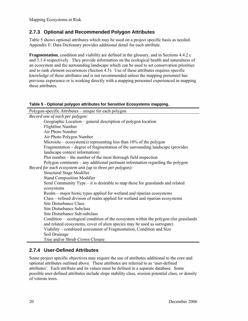
2.7.3 Optional and Recommended Polygon Attributes Table 5 shows optional attributes which may be used on a project specific basis as needed. Appendix E: Data Dictionary provides additional detail for each attribute.
Fragmentation, condition and viability are defined in the glossary, and in Sections 4.4.2.c and 3.1.4 respectively. They provide information on the ecological health and naturalness of an ecosystem and the surrounding landscape which can be used to set conservation priorities and to rank element occurrences (Section 4.5). Use of these attributes requires specific knowledge of these attributes and is not recommended unless the mapping personnel has previous experience or is working directly with a mapping personnel experienced in mapping these attributes.
Table 5 - Optional polygon attributes for Sensitive Ecosystems mapping. Polygon-specific Attributes – unique for each polygon Record one of each per polygon:
Geographic Location – general description of polygon location Flightline Number Air Photo Number Air Photo Polygon Number Microsite – ecosystem(s) representing less than 10% of the polygon Fragmentation – degree of fragmentation of the surrounding landscape (provides landscape context information) Plot number – the number of the most thorough field inspection Polygon comments – any additional pertinent information regarding the polygon
Record for each ecosystem unit (up to three per polygon): Structural Stage Modifier Stand Composition Modifier Seral Community Type – it is desirable to map these for grasslands and related ecosystems Realm – major biotic types applied for wetland and riparian ecosystems Class – refined division of realm applied for wetland and riparian ecosystems Site Disturbance Class Site Disturbance Subclass Site Disturbance Sub-subclass Condition – ecological condition of the ecosystem within the polygon (for grasslands and related ecosystems, cover of alien species may be used as surrogate) Viability – combined assessment of Fragmentation, Condition and Size Soil Drainage Tree and/or Shrub Crown Closure
2.7.4 User-Defined Attributes Some project specific objectives may require the use of attributes additional to the core and optional attributes outlined above. These attributes are referred to as ‘user-defined attributes’. Each attribute and its values must be defined in a separate database. Some possible user-defined attributes include slope stability class, erosion potential class, or density of veteran trees.
20 December 2006

Mapping Ecosystems at Risk
2.8 Spatial Digital Data Capture In this phase of the mapping, the polygons mapped by ecologists or bioterrain specialists on aerial photographs are captured through the process of mono-restitution. Mono-restitution is the digital transfer of features by digitising directly from aerial photographs using TRIM control points to georeference the data, and TRIM digital elevation models to correct for slope. The process allows for adjustments in polygon shape and size related to the third dimension. A series of standard routines are applied to determine the quality and accuracy of the mapping.
Other imagery such as satellite photography or infrared imagery can also be used, as could the more recently developed ‘heads up’ or 3-D mapping methods using programs such as Softcopy. In this case, the ecologist works within a digital environment, digitizing linework using digital orthophotos and a digital elevation model.
Ecosystems are represented visually on maps and the digital data required to produce this representation is maintained according to standards outlined in the Standard for Terrestrial Ecosystem Mapping (TEM) Digital Data Capture in British Columbia (Resources Inventory Committee 2000b) and Errata No. 1.0 (Resources Inventory Standards Committee 2004b). The required mapping base is the Terrain Resource Information Management (TRIM) provincial standard. The digital spatial databases must adhere to the TEM Digital Capture Standards (files must be in Arc/Info format and projected in Albers).
2.9 Biogeoclimatic (BGC) and Ecosection Linework For most areas where Sensitive Ecosystems are likely to be mapped, medium-scale (generally 1:50 000) BGC mapping is available through the Ministry of Forests and mapping should use existing lines. For more information, see http://www.for.gov.bc.ca/hre/becweb/resources/maps/index.html. Where medium-scale BGC mapping does not exist, BGC mapping must follow the TEM Standard (Resources Inventory Committee 1998b, Section 6) and be approved by the applicable Ministry of Forests’ regional ecologist prior to the production and submission of final ecosystem mapping. Where BGC lines and Ecosection lines are contiguous, Ecosection lines are usually adjusted to follow new BGC lines.
2.10 Accuracy Assessment and Quality Assurance It is desirable to determine a map’s thematic accuracy. Accuracy Assessments are completed by a qualified third party. Meidinger (2003) provides a protocol for obtaining statistically valid scores to rate the thematic accuracy of ecosystem maps. Quality assurance may be managed by having the contractor sign the reports assuring the quality of the deliverables.
2.11 Reporting The report should follow the principles of scientific reporting. The report accompanying the mapping provides the following information on Sensitive and Other Important Ecosystems in the study area:
1. Acknowledgements, including any funding sources.
December 2006 21

Mapping Ecosystems at Risk
2. Abstract – a summary of the contents of the report.
3. Introduction – describes the rationale for the project, objectives for the study, contents of the report, a description of the study area, including its ecological importance and provincial or North American context, a table and description of what Sensitive and Other Important Ecosystems occur in the study area, a section on ‘Ecosystems of Concern’ – the importance and need for concern about Sensitive Ecosystems, and a section on ‘Impacts of Concern’;
4. Methods and Limitations – describe mapping methods, spatial data capture methods, field sampling (a table showing the number and types of field inspections for each class), and mapping limitations;
5. Results – describes inventory results including the overall status of Sensitive and Other Important Ecosystems in the study area (see Table 6 below as an example, other results such as areas of high viability by class or subclass, areas of red and blue-listed ecological communities can be included depending on project objectives);
6. Planning and Management – provides planning and management recommendations for conservation that are applicable to all Sensitive and Other Important Ecosystems;
7. Ecosystem Chapters - provide a chapter for each Sensitive and Other Important Ecosystem class with a description of the ecosystem (including a description of the vegetation and environmental description of the class and subclass), a vegetation table showing plant species and abundance for each subclass (see Table 20 and Table 21 in Appendix F: Example Vegetation Tables for SEI Reports for one possible format), importance (including a list of ecological communities at risk of each ecosystem), status (including a graph showing the percentage of study land area for each subclass), and management recommendations for the ecosystem; and
8. Recommendations for future directions including updating products.
9. Appendix with TEM codes and short descriptions of TEM units.
10. A Conservation Manual including:
a. ‘What local governments can do’
b. ‘What landowners and citizens can do’
c. ‘What senior governments can do’
Each of the sections of the Conservation Manual may be comprehensive or may simply provide updates to or make reference to existing SEI reports and conservation manuals in ecologically similar areas, and they should provide project specific information.
22 December 2006

Mapping Ecosystems at Risk
Table 6 - Area of Sensitive and Other Important Ecosystems in the Central Okanagan SEI (from Iverson and Cadrin 2003). Area (ha) Percent of Study Area Sensitive Ecosystems (SE) Broadleaf Woodland 353 6.2 Grassland 952 16.6 Old Forest 24 0.4 Riparian 87 1.5 Sparsely Vegetated 358 6.3 Coniferous Woodland 56 1.0 Wetland 72 1.3 Total SE 1901 33.2 Other Important Ecosystems (OIE) Disturbed Grassland 1350 23.6 Mature Forest 187 3.3 Total OIE 1536 26.8 TOTAL SEI and OIE 3347 60.0
2.12 Digital Data Deliverables The final submission of seamless data and all associated files must be made in one data transfer. The files must be zipped into one file and delivered to the Ministry of Environment ftp site at ftp://ftp.env.gov.bc.ca/pub/incoming/SEI/. Anonymous login will be used to access the ftp site. The file should be named: sei_<BAPID>.zip
The Business Area Project Identification number <BAPID> must be requested from the Ministry of Environment at the onset of the project. When submitting a request for BAPID the following information should be included in the body of the email:
• Project Name:
• FIA Contract No (if applicable):
• MoE Region:
• Scale of Mapping:
• Location (i.e. mapsheets, landscape units, etc.):
• Client:
• Mapping Consultant:
• Start date:
BAPID requests should be sent to: [email protected]. The province should also be notified at this address whenever final data is posted to the ftp site. The subject line of the email should include the line “Request for BAPID” or “<BAPID>final deliverables.”
December 2006 23

Mapping Ecosystems at Risk
2.12.1 Spatial Data Spatial data deliverables include a SEI polygon coverage (SEI_<BAPID>_ecp.e00) and a plot location coverage (SEI_<BAPID>_eci.e00) as ARC/INFO single precision export files.
All spatial files should be accompanied by meta-data. Provincial standards for Arc files can be found at http://srmwww.gov.bc.ca/gis/arcmetadata.html. If the ecosystem digital map is stored in a format other than ARC/INFO, it is the responsibility of the client to ensure the data is converted into the standard format. Export files must be created with the ‘NONE’ compression option (produces readable ASCII).
Projects captured from stereo pairs using mono-restitution or other methodologies will include reports and materials necessary for quality control and assurance as listed below.
1. The original or a colour-copy of typed aerial photographs and update photos with controls marked.
2. A digital file containing control points in ASCII (CSV) format. This control point file shall contain point numbers, X, Y, Z, coordinates (to three decimal places).
3. All original source materials provided by the Ministry, including TRIM prints and diapositives, along with TRIM digital control.
4. Mono-restitution set up (digital) reports for each model (See Table 6-1 in Resources Inventory Standards Committee 2004b).
2.12.2 Non-Spatial Data Deliverables
2.12.2.a Non-Spatial Attribute Databases
The first three databases listed below are mandatory deliverables. The user-defined database is optional depending on project specifications. File naming follows TEM Digital Data Capture errata (Resources Inventory Standards Committee 2004b) with ‘sei’ replacing all occurrences of ‘tem’.11
1. SEI Project Database (SEI_<BAPID>_mta.csv): This database includes the project meta-data and must follow the format and contain all data outlined in Appendix E: Data Dictionary.
2. SEI Polygon Database (SEI_<BAPID>_ecp.csv): This database includes ecosystem attributes and must contain all mandatory fields indicated in Appendix E: Data Dictionary.
3. SEI Field data (SEI_<BAPID>_eci.mdb): Full plots, GIFs, and visual checks must be submitted as VENUS files. Information from the Conservation Evaluation Form is entered as “notes” into VENUS.
4. SEI User Defined database (SEI_<BAPID>_usr.csv): This database defines project specific attributes and is required if user-defined attributes are applied.
11 For SEIs from TEM and PEM, see sections on Digital Data Deliverables.
24 December 2006
Mapping Ecosystems at Risk
5. SEI User Defined attributes database (SEI_<BAPID>_uda.csv): This database includes the ECP_TAG and the user-defined attributes for each polygon.
2.12.2.b Map Legend
Where hard copy maps are produced, the map legend is required in Portable Document Files (SEI_<BAPID>_ml.pdf) format. Section 2.13.3 describes the contents of map legends.
2.12.2.c Reporting
The final report is submitted in Portable Document Files (SEI_<BAPID>_rpt.pdf) format. All figures and photos should be embedded and saved within the document. Graphics and other inserts should not be linked to the report as separate documents.
2.12.2.d Plot Cards and Air Photos
Original or copies of plot cards and typed air photos must be delivered to:
Conservation Data Centre, Ministry of Environment
2.12.2.e Quality Assurance (QA) and Accuracy Assessment (AA) Reporting
Quality Assurance or Accuracy Assessment reviews must be submitted documenting all steps in the QA or AA review in a report in Portable Document Files (.pdf) format.
2.12.2.f Data Acceptance/Sign-off
All final deliverables must conform to the standards discussed in this document and must pass data verification rules.
2.13 Map Production It is recommended that the SEI map display Sensitive Ecosystems in each polygon using a dot-density theme. The dot-density display visually indicates the component sensitive ecosystem classes within each polygon. A polygon number is the minimum polygon label that allows the user to locate detailed ecosystem information from the map legend or the digital database; full labels (see Figure 1) are preferred where possible. A tool may be created to allow SEI map labels to be generated from the SEI database.
This section describes the recommended standards for SEI map symbols and lines when producing hardcopy or pdf maps. These are similar to TEM mapping standards (Resources Inventory Committee 1998b), with some modifications.
2.13.1 Polygon Labels Each polygon should be labelled with the map polygon number and a polygon label with deciles, SE class and SE subclass (see Figure 1; colours are used for illustration purposes only).
December 2006 25

Mapping Ecosystems at Risk
Decile 1 (40%)
Decile 2 (40%)
Decile 3 (20%)SE Class 1
SE Class 2
SE Class 3
Subclass 3
RI:gu OF:co SV:ro
Subclass 1
4 4 2
Sensitive Ecosystem Map Label
Subclass 2
Decile 1 (40%)
Decile 2 (40%)
Decile 3 (20%)SE Class 1
SE Class 2
SE Class 3
Subclass 3
RI:gu OF:co SV:ro
Subclass 1
4 4 2
Subclass 2
Sensitive Ecosystem Map Label
Figure 1 - Compound map unit label.
2.13.2 Map Linework The following standardized polygon boundary line weights should be used for final presentation of Sensitive Ecosystems mapping:
• Ecosection unit lines – 1.20 mm (dashed green)
• Biogeoclimatic unit lines – 0.80 mm (red)
• Polygon boundaries – 0.35mm (black)
• Project boundary lines – 1.20 mm (black)
• Mapsheet neatline – 0.25 mm (black)
2.13.3 Map Legend and Map Surround The map legend provides a summary of all map units, map symbols, and map lines with other supporting information including survey objectives, survey intensity, location, field sampling, other data sources, aerial photograph reference numbers, and map credits.
As a minimum, the items in Table 7 should be included in all SEI map legends. Layout can vary and additional information may be added if required.
26 December 2006

Mapping Ecosystems at Risk
Table 7- Minimum data to be included on SEI map legends.
Item Minimum Requirements Title Include:
1. Study area name 2. Map sheet number/s (NTS, BCGS) 3. Map scale 4. Date
Introduction (project summary)
Include: 1. Objectives of the mapping project 2. Rationale for the project 3. Ecological significance of the study area 4. A brief description of each Sensitive and Other Important
Ecosystem class 5. Summary of methods including mapping standards, survey
intensity level 6. Summary of data limitations
Map Label Format Provide one or more examples of a polygon label Map Symbols Provide examples of all line types and map symbols Ecosystem Classes/subclasses
List and describe all Sensitive and Other Important Ecosystem classes and subclasses including name, two-letter codes, and a brief definition.
Data Sources Include lists of all data sources in the project: 1. aerial photographs (year, scale, all photo numbers, colour or black
and white) 2. all previously available data and maps such as vegetation resources
inventory, satellite imagery, soils maps, bedrock geology maps, base maps, etc.
3. percent polygons or ha per inspection field verified 4. number and type of samples
Credits Include: 1. names of all mapping personnel and field personnel 2. name of project supervisor 3. names of quality assurance personnel and reviewers 4. co-ordinating and funding agencies 5. GIS personnel
Citation Provide the citation as it should be referenced in other reports. Index Map Small scale map of 1:20 000 grid, showing location of map as well as
small scale map of province showing location of study area. TEM Units It is optional to provide a map legend including TEM codes. If
included the following is required: a table listing TEM codes and brief descriptions and a list and definition of structural stages together with a table of TEM labels for each polygon.
December 2006 27

Mapping Ecosystems at Risk
3 Modelling SEI SEI mapping can be modelled from ecosystem mapping products including Terrestrial Ecosystem Mapping (TEM), Predictive Ecosystem Mapping (PEM), and Broad Ecosystem Inventory (BEI).
3.1 Terrestrial Ecosystem Mapping This inventory, sampling, and mapping method (Resources Inventory Committee 1998b) is suitable for mapping all ecosystems including ecosystems at risk. TEM can provide an effective base for developing an SEI map, especially with a few refinements to standard mapping methods.
Several medium to large scale mapping projects have been completed with the specific objectives of ecosystem conservation, management and restoration for local government and park planning. (e.g., BC Ministry of Environment, Lands and Parks and BC Conservation Foundation 1999; Iverson et al. 2004).
If you are starting a new TEM project which will be used to theme SEI, the following sections discuss areas of TEM which require adjustments in order to achieve the requisite documentation of ecosystems at risk and Sensitive Ecosystems.
If you are using an existing TEM to theme SEI, methods are described in Section 3.1.5 below.
3.1.1 Bioterrain mapping Adjust bioterrain linework to maintain continuity of polygons along continuous hydrologic corridors and other water bodies. Water courses are commonly bisected in terrain mapping; this reduces the effectiveness of highlighting sensitive riparian components of the landscape.
Delineate smaller polygons for Sensitive Ecosystems to produce more simple rather than complex polygons where possible, or, at minimum, ensure that Sensitive Ecosystems occupy a minimum of 10% of the polygon area. Delineate polygons to separate modified portions of ecosystems from unmodified ecosystems (e.g., cutblocks, urban, and agricultural areas).
3.1.2 Sampling strategy Naturally rare ecological communities are often poorly documented and there are many ecosystems at risk that have never been sampled or documented.
Previously undescribed ecosystems should be sampled at a higher intensity, primarily with full and ground inspection plots, to increase our knowledge and understanding of them and to assist in determining their conservation status. Sampling should be directed towards Sensitive and Other Important Ecosystems.
Proportions of plot types should be adjusted according to the study area size, existing data, and the possible scope of undocumented ecosystems that may occur in the study area. Higher
28 December 2006

Mapping Ecosystems at Risk
proportions of full and ground inspection plots should be used for smaller study areas, areas with limited existing data, and areas with the potential for undocumented ecosystems. The sampling strategy should be flexible to allow for adjustments when new ecosystems are encountered during field work.
Where available, producing themes from other map sources can help direct sampling. The sampling plan should identify potential areas of unique environmental specificity using bedrock mapping, bioterrain mapping, biogeoclimatic mapping, TRIM mapping, and interviews with local naturalists, and ecologists familiar with the area.
3.1.3 New ecosystem classification For naturally rare ecosystems that have not been documented or classified, develop new TEM unit classifications rather than lumping or grouping them within an existing classification (see Table 2 - Areas of atypical environmental characteristics (from Maxwell et al. 1993).). Project ecologists should contact the CDC and regional Ministry of Forests and Range research ecologist prior to sampling an area to be aware of such possibilities. Surveyors should also inform the CDC if they locate samples which cannot be assigned to any previously described ecological community. This information may lead to the recognition and documentation of new ecological communities. New Sensitive Ecosystem units and their codes must be submitted to and approved by the CDC ecologist prior to use. Data should remain connected to a polygon number so that the polygon label or attribute can be updated if the sample results in the description of an ecosystem type.
3.1.4 Additional Attributes Table 8 shows the optional attributes recommended in addition to core TEM attributes. These attributes are needed to model condition and viability of at-risk ecosystems. Seral community type is a recommended attribute for grassland and related ecosystems because it is relevant to determine the Sensitive Ecosystem subclass. Alternatively, condition ratings, based on the percent cover of alien plant species, can be used to assign grasslands and related ecosystems to the ‘disturbed’ subclass (See Section 2.4.2 for definitions of condition classes in grasslands and related ecosystems). Stand composition modifiers are necessary to determine the Sensitive Ecosystem subclass for forested ecosystems (e.g., broadleaf, mixed, coniferous). Fragmentation, condition and viability are optional attributes that are unique to mapping ecosystems at risk. They are defined in detail in Section 4.4.2. They provide information on the ecological health and naturalness of an ecosystem and the surrounding landscape which can be used to set conservation priorities and to rank element occurrences (Sections 4.1 to 4.6).
December 2006 29

Mapping Ecosystems at Risk
Table 8 - Additional polygon attributes for terrestrial ecosystem mapping used to derive an SEI map. Polygon-specific Attributes – unique for each polygon Record one of each of the following elements or classes per polygon:
Fragmentation – degree of fragmentation of the surrounding landscape (provides landscape context information) – optional
Record for each of the up to three ecosystem units per polygon Structural Stage Modifier – optional Seral Community Type – recommended for grasslands and related ecosystems Site Disturbance Class – optional Site Disturbance Subclass – optional Site Disturbance Sub-subclass – optional Stand Composition Modifier – required Condition – ecological condition of the ecosystem within the polygon; optional Viability – combined assessment of Fragmentation, Condition, and Size; optional
3.1.5 Developing the SEI Theme
3.1.5.a At-risk and Sensitivity Analysis
Each TEM unit is individually assessed by the project ecologist for ecological sensitivity and at-risk status. Criteria for ecological sensitivity include: susceptibility to hydrological changes, shallow soils, susceptibility to erosion, sensitivity to human disturbance, spread of invasive alien plants, and environmental specificity (see Table 2 - Areas of atypical environmental characteristics (from Maxwell et al. 1993).). Criteria for at-risk status include the status determined by the CDC and proposed status (provided by the project ecologist) for ecosystems presently not assessed by the CDC. The status is based on the local and provincial distribution of the ecosystem (especially in an undisturbed state) and threats to the ecosystem. An ecosystem unit determined to be ecologically sensitive or at-risk is assigned to the applicable Sensitive Ecosystem Class and Subclass.
Where an ecosystem unit could be assigned to more than one Sensitive Ecosystem unit, it is assigned to the more sensitive unit. Within each class, subclasses are identified which further refine these groupings, reflecting similarities in ecological processes, landscape positions, and vegetation characteristics. Examples of these classes are described in Appendix D: SEI Map Codes, Map Units and Descriptions. Table 9 below shows an example assignment of TEM units to Sensitive Ecosystem units for the Central Okanagan SEI.
Terrestrial ecosystems not considered at-risk or ecologically sensitive, or that do not meet minimum size criteria for each project12, are not assigned to a Sensitive Ecosystem unit.
12 Mature Forest (MF) is mapped as an Other Important Ecosystem and must meet size criteria related to overall biodiversity values. MF is mapped when it occurs as larger patches as conservation biology recognizes that larger forest patches generally support more species than smaller forest patches by retaining landscape connectivity and habitat for species that require larger home ranges.
30 December 2006

Mapping Ecosystems at Risk
Table 9 – Some Sensitive Ecosystem units and related Terrestrial Ecosystem Mapping (TEM) units for the Central Okanagan SEI (from Iverson and Cadrin 2003).
SEI Class, subclass
SEI Code
TEM Unit TEM Map Unit Code13
Subzone / Site Series
Wetland, WN:ms Bulrush marsh BM IDFxh1 /0014
marsh Baltic rush marsh-meadow BR IDFxh1 /00 Common spikerush marsh CS IDFxh1 /00 Cattail marsh CT IDFxh1 /00
PPxh1 /00 Sedge marsh SM IDFxh1 /00 Wetland, swamp WN:sp Willow – Sedge wetland WS IDFxh1 /09 Riparian, bench
RI:fp Trembling aspen – Mock orange – Choke cherry riparian
AOa, AOt IDFxh1 /00
Black cottonwood – Douglas-fir – Common snowberry – Red-osier dogwood riparian
CDa, CDac, CDct, CDt IDFxh1 /00
Douglas-fir – Water birch – Douglas maple DMa, DMct, DMt PPxh1 /08 Douglas-fir – Ponderosa pine – Snowberry – Spirea DSa, DSt IDFxh1 /07 Ponderosa pine – Black cottonwood – Snowberry
riparian PAa, PAac, PAt PPxh1 /00
Western red cedar – Douglas-fir – False Solomon’s Seal
RSa, RSac IDFxh1 /00
Hybrid white spruce – Douglas-fir – Douglas maple – Dogwood
SDa, SDac, SDt IDFxh1 /08
Old Forest, OF:co Douglas-fir – Ponderosa pine – Pinegrass DP 7C IDFxh1 /01 coniferous Douglas-fir – Ponderosa pine – Snowberry – Spirea DS 7C (except those
with ‘a’, ‘g’, or ‘t’ modifiers)
IDFxh1 /07
Douglas-fir – Ponderosa pine – Bluebunch wheatgrass – Pinegrass
DW 7C IDFxh1 /03
Douglas-fir – Ponderosa pine – Saskatoon – Mock orange
FO 7C IDFxh1 /00
Douglas-fir – Ponderosa pine – Bluebunch wheatgrass – Balsamroot
PB 7C IDFxh1/02
Douglas-fir – Ponderosa pine – Snowbrush – Pinegrass
SP 7C IDFxh1 /04
Grassland, GR:gr Rough fescue – Bluebunch wheatgrass FB PPxh1 /00 grassland Rough fescue – Cladina FC IDFxh1 /00 Idaho fescue – Bluebunch wheatgrass FW, FW:$nb IDFxh1 /91 Giant wildrye GW PPxh1 /00 Big sagebrush – Bluebunch wheatgrass – Balsamroot WA (no seral
community) IDFxh1 /92
Bluebunch wheatgrass – Balsamroot WB (no seral community)
IDFxh1 /93 PPxh1 /00
3.1.5.b Ecosystem-based Resource Rating Modelling Tool
Once the appropriate Sensitive Ecosystem classes and subclasses are identified, TEM units are grouped into SEI units using the Ecosystem-based Resource Rating Modelling Tool (ERM) developed by the Ecosystem Information group of the Ministry of Environment to rate ecosystems for wildlife habitat values (http://srmwww.gov.bc.ca/wildlife/whr/sta.html).
The ERM system tool allows ratings, or in this case, SEI classes and subclasses, to be assigned to each TEM unit in a ratings table. TEM units that are not assigned to a sensitive
13 All site modifier combinations, structural stages, and seral associations are included unless otherwise noted. Seral stages are indicated by the two letters following a ‘$’ (e.g., $kw). Structural stages are indicated by a number (e.g. ‘7’). Structural stage stand composition modifiers are indicated by a capital letter after the number (e.g., ‘C’ in ‘7C’). See Volume 2 (Iverson et al. 2003) for descriptions of site modifiers, structural stages, seral associations, and TEM units. 14 ‘00’ Site Series are those ecosystem units that have not been classified as site series in BEC.
December 2006 31

Mapping Ecosystems at Risk
ecosystem class should be rated non-sensitive. The ERM also provides for a variety of options for presenting the themed results, allowing for the inclusion of up to three components within a polygon. Examples of ratings tables used to convert TEM units to SEI units can be found in Appendix G: Example SEI Ratings Table.
3.1.5.c Modelling Condition and Fragmentation
Where condition and fragmentation were not mapped as additional attributes in the TEM project, these attributes can sometimes be modelled from the ecosystem map and TRIM base data. Any formula or algorithm used to model fragmentation, condition, or viability must be approved by the CDC ecologist.
Fragmentation: analyze TRIM data for roads, TEM data for urban, agricultural, and other anthropogenic areas, and analyze harvesting history and forest age from Vegetation Resources Inventory (forest cover) data.
Condition: for forested ecosystems, analyze ecosystem data by size and structural stage; for grasslands, analyze by size and seral community and adjacency to urban, agricultural or other anthropogenic areas; for other non-forested ecosystems, analyze based on adjacency to anthropogenic areas.
Viability: the elements used to evaluate fragmentation and condition, and the size of the occurrence of the ecosystem15 can be used together to model the viability of an ecosystem.
3.1.6 Digital Data Deliverables Digital data deliverables are the same as those outlined in TEM Digital Data Capture Standards (Resources Inventory Committee 2000b; http://ilmbwww.gov.bc.ca/risc/pubs/teecolo/temcapture/index.htm) and Standards for Terrestrial Ecosystem Mapping (TEM) Digital Data Capture in British Columbia, Version 3.0 (2000), Errata No. 1.0 (Resources Inventory Standards Committee 2004b; http://ilmbwww.gov.bc.ca/risc/pubs/teecolo/temcapture/assets/temddc_v3_errata1.pdf). TEM digital data deliverables are not re-submitted as part of an SEI project unless an older TEM project was altered or upgraded for use in the SEI.
For new TEM projects used for SEI, the TEM database must include the required optional attributes as noted in Section 3.1.4 when delivering the deliverables to the TEM data custodian.
3.1.6.a SEI Ratings Table
The SEI Ratings table is required to be delivered to the SEI data custodian. The ratings table must contain a column with the SEI class ‘rating’ (e.g., RI), a column with the SEI subclass ‘rating’ (e.g., fp), and a column with the combined SEI class and subclass (e.g., RI:fp). The file is named ‘sei_<BAPID>_rt.xls’.
15 The size of the ecosystem occurrence relative to typical size range of the ecosystem in an undisturbed landscape.
32 December 2006

Mapping Ecosystems at Risk
3.1.6.b SEI Databases
Separate SEI databases are created in addition to the standard TEM deliverables. The first three databases listed below are mandatory deliverables. The user-defined database is optional depending on project specifications. File naming follows TEM Digital Data Capture errata (Resources Inventory Standards Committee 2004b) with ‘sei’ replacing all occurrences of ‘tem’.16
1. SEI Project Database (SEI_<BAPID>_mta.csv): This database includes the project meta-data and must follow the format and contain all data indicated in Appendix E: Data Dictionary.
2. SEI Polygon Database (SEI_<BAPID>_ecp.csv): This database includes ecosystem attributes and must contain all mandatory fields indicated in Appendix E: Data Dictionary.
3. SEI Field data (SEI_<BAPID>_eci.mdb): Full plots, GIFs, and visual checks must be submitted as VENUS files unless already submitted as complete files as a TEM deliverable. Information from the Conservation Evaluation Form is entered into as “notes” into VENUS.
4. SEI User Defined database (SEI_<BAPID>_usr.csv): This database defines project specific attributes and is required if user-defined attributes are applied.
5. SEI User Defined attributes database (SEI_<BAPID>_uda.csv): This database includes the ECP_TAG and the user-defined attributes for each polygon.
3.1.7 Map Production Where an SEI theme map intended for presentation is created, the map should display Sensitive Ecosystems in each polygon using a dot-density theme. The map should follow the map layout outlined in Section 2.13 with the exception of Polygon Labels (Section 2.13.1). A polygon number is the minimum polygon label; full labels are preferred where possible. If full labels are displayed, NS is used to code non-sensitive ecosystem components. A tool may be created to allow SEI map labels to be generated from the TEM database and SEI ratings table. The map legend can include a legend of TEM units, modifiers, structural stages, and TEM labels for each polygon.
3.2 Predictive Ecosystem Mapping Predictive Ecosystem Mapping (PEM) is a process of using available spatial data and knowledge tables and creating new spatial data to automate the generation of ecosystem maps. Typically, map layers are spatially overlaid and the resulting attributes are input into a knowledge base used to infer ecosystems. At times, some site series are lumped and more generalized site units are mapped than in TEM (Resources Inventory Committee 1999).
PEM is suitable for strategic level ecosystem mapping and can provide a base for developing a broad Sensitive Ecosystem map, particularly with a few refinements to standard mapping methods. PEM is sometimes more limited than TEM for delineating naturally rare
16 For SEIs from TEM and PEM, see section Digital Data Deliverables.
December 2006 33

Mapping Ecosystems at Risk
ecosystems. Although standard PEM knowledge tables are not generally designed to identify the unusual or uncommon ecosystem types, they can sometimes be adapted to identify uncommon combinations. Polygons containing these uncommon combinations may need to have attributes assigned to them using aerial photograph interpretation.
If you are starting a new PEM project which will be used to theme SEI, Section 3.2.1 below discusses how to adjust PEM to achieve the requisite documentation of ecosystems at risk and other Sensitive Ecosystems.
If you are starting a PEM project which will be used to directly create an SEI, one possible approach is discussed in Section 3.2.2.
If you are using an existing PEM to theme SEI, apply same methods as described for TEM in Section 3.1.5 above.
3.2.1 Modelling SEI maps from PEM The sampling strategy for new PEM projects should follow Section 3.1.2; new units are developed as outlined in Section 3.1.3.
For new PEM projects that will be used to develop an SEI theme, additional attributes are required to apply PEM to ecosystems at risk and SEI mapping (see Section 3.1.4 above). Where the PEM project includes a bioterrain map base, the same recommendations for modifications in TEM apply (see Section 3.1.1 above).
3.2.1.a Developing the SEI Theme
The SEI theme is developed as outlined in Section 3.1.5.
3.2.1.b Ecosystem-based Resource Rating Modelling Tool
Once the appropriate Sensitive Ecosystem classes and subclasses are identified, PEM units are grouped into SEI units using the Ecosystem-based Resource Rating Modelling Tool (ERM) developed by Ecosystem Information group of the Ministry of Environment http://srmwww.gov.bc.ca/wildlife/whr/sta.html. See Section 3.1.5.b for further details.
3.2.1.c Modelling Condition and Fragmentation
Condition and fragmentation can sometimes be modelled from the ecosystem map and TRIM base data. Any formula or algorithm used to model fragmentation, condition, or viability must be approved by the CDC ecologist. See Section 3.1.5.c for further details.
3.2.2 Using PEM Directly to Map Sensitive Ecosystems An alternative to modelling an SEI map from an existing PEM is to design a specific knowledge base to predict the probability of a particular Sensitive Ecosystem occurring in a polygon using base map layers and other resource information. PEM knowledge tables need to be designed to identify uncommon combinations of attributes which may include some at-risk ecosystems or other Sensitive Ecosystems. Polygons containing these uncommon combinations may need to have attributes assigned to them using aerial photograph interpretation.
34 December 2006

Mapping Ecosystems at Risk
A pilot project was tested by Ketcheson et al. (2002) to predict the potential occurrence of ecosystems at risk. The information was applied to the model by using bedrock geology maps, soils maps, Biogeoclimatic and Ecosection mapping and Forest Cover mapping. TRIM base maps were also used to determine locations of wetlands and riparian corridors. The mapping did not assign site series or ecological community to the polygons. Ecosystem units were equivalent to a Sensitive Ecosystems Inventory mapped to the Class level.
3.2.3 Digital Data Deliverables Digital data deliverables are the same as those outlined in Standards for Predictive Ecosystem Mapping (PEM) Digital Data Capture Version 1.0 (Resources Inventory Committee 2000a; http://ilmbwww.gov.bc.ca/risc/pubs/teecolo/pemcapture/index.htm) and Standards for Predictive Ecosystem Mapping (PEM) Digital Data Capture in British Columbia, Version 1.0 (2000), Errata No. 1.0 (Resources Inventory Standards Committee 2004a; http://ilmbwww.gov.bc.ca/risc/pubs/teecolo/pemcapture/assets/pemddc_v1_errata1.pdf) . PEM digital data deliverables are not re-submitted as part of an SEI project unless an older PEM project was altered or upgraded for use in the SEI.
Where the project is a new PEM designed to model SEI, the database must include any additional attributes as noted in Section 3.1.4 when submitting deliverables to the PEM data custodian.
3.2.3.a SEI Ratings Table
Where the SEI was modelled from a PEM, the SEI Ratings table is a required deliverable. The ratings table must contain a column with the SEI class ‘rating’ (e.g., RI), a column with the SEI subclass ‘rating’ (e.g., gu), and a column with the combined SEI class and subclass (e.g., RI:gu). The file is named ‘sei_<BAPID>_rt.xls’.
3.2.3.b SEI Databases
Separate SEI databases are created in addition to the standard PEM deliverables. The first three databases listed below are mandatory deliverables. The user-defined database is optional depending on project specifications. File naming follows PEM Digital Data Capture errata (Resources Inventory Standards Committee 2004a) with ‘sei’ replacing all occurrences of ‘pem’.17
1. SEI Project Database (SEI_<BAPID>_mta.csv): This database includes the project meta-data and must follow the format outlined in and contain all data indicated in Appendix E: Data Dictionary.
2. SEI Polygon Database (SEI_<BAPID>_ecp.csv): This database includes ecosystem attributes and must follow the format outlined in and contain all mandatory fields indicated in Appendix E: Data Dictionary.
3. SEI Field data (SEI_<BAPID>_eci.mdb): Full plots, GIFs, and visual checks must be submitted as VENUS files. Information from the Conservation Evaluation Form is entered into as “notes” into VENUS.
17 For SEIs from TEM and PEM, see section Digital Data Deliverables.
December 2006 35
Mapping Ecosystems at Risk
4. SEI User Defined database (SEI_<BAPID>_usr.csv): This database defines project specific attributes and is required if user-defined attributes are applied.
5. SEI User Defined attributes database (SEI_<BAPID>_uda.csv): This database includes the ECP_TAG and the user-defined attributes for each polygon.
3.2.4 Map Production Where an SEI theme map intended for presentation is created from an existing PEM, the map should display Sensitive Ecosystems in each polygon using a dot-density theme together with the polygon number. The map should follow the layout outlined in Section 2.13 with the exception of Polygon Labels (Section 2.13.1). A polygon number is the minimum polygon label; full labels are preferred where possible. If full labels are displayed, NS is used to code non-sensitive ecosystem components. The map legend can include a legend of PEM units, modifiers, structural stages, and PEM labels for each polygon.
Where a predictive SEI map is created from a SEI knowledge table, map production should follow the layout outlined in Section 2.13, including polygon labels.
3.3 Broad Ecosystem Mapping A Broad Ecosystem Unit (BEU) is an area of a landscape that supports a distinct type of vegetation cover at climax or distinct non-vegetated cover. BEUs are designed to provide an ecological framework for wildlife habitat suitable for broad planning initiatives (Resources Inventory Committee 1998a). Each BEU includes many BEC site series and associations, and can only be used to identify general areas of the landscape where there may be a concentration of ecosystems at risk. BEUs have been mapped across the province of British Columbia at a scale of 1:250,000 to create a Broad Ecosystem Inventory (BEI) map.
Modelling from the BEI mapping may be useful for delineating broad areas which can be flagged for potential occurrences of ecosystems at risk and other Sensitive Ecosystems. Each BEI ecosystem can be assessed for at-risk status. This method of identifying areas of potential ecosystems at risk was piloted for the Central Coast Local Resources Management Plan (McLennan 2000).
Using the correlation tables in Appendix A of the BEI standards, the authors determined the number of ecological communities (based on site series distributions) potentially occurring within a BEU and rated each BEU very high, high, medium or low for potential occurrence of ecosystems at risk (Table 10). Within each biogeoclimatic subzone or variant, the total number of site series in a BEU is divided by the number of site series that potentially contain red- or blue-listed ecological communities. Sensitivity could be assessed in a similar manner and the resultant map could portray both Sensitive Ecosystems and ecological communities at risk. The mapping is limited by scale and resolution. Many ecosystems will be submerged within the larger polygons mapped at 1:250,000. However, this method can be useful for the identification of geographic areas requiring more detailed work.
36 December 2006

Mapping Ecosystems at Risk
Table 10 - Ecosystems at risk probability classes (adapted from McLennan 2002).
Probability Class Probability Very High (4) The mature/old forest and non-forested ecological communities of all site
series in the BEU are blue- or red-listed. High (3) The mature/old Forest and non-forested ecological communities of 50-99%
site series in the BEU are blue or red-listed. Moderate (2) The mature/old forest or non-forested ecological communities of 1-49% of
all site series in the BEU are blue or red-listed. Low (1) No mature/old forest or non-forested ecological communities of site series in
the BEU are blue or red-listed.
3.4 Limitations on Using Pre-existing Map Products There are several limitations on using pre-existing map products. Bioterrain polygon delineation in pre-existing TEM and PEM products commonly does not maintain continuous polygons along hydrologic corridors and other water bodies; this reduces the effectiveness of highlighting sensitive riparian components of the landscape. Often, smaller Sensitive Ecosystems may be incorporated into larger polygons and, where they occupy less than 10% of the polygon, are not included in the map database. In some cases, many non-forested ecosystems such as grasslands may have been mapped too generally to be useful for deriving an SEI map. Naturally rare ecosystems tend to be lumped in with other ecosystems rather than being classified as separate ecosystem units. Finally, the sampling plan likely had different objectives and Sensitive Ecosystems may have been sampled less intensively, potentially lowering the reliability for this portion of the product.
3.5 Accuracy Assessments Some previously completed ecosystem maps may have completed accuracy assessments. Accuracy assessments are completed for a specific set of map attributes, and accuracy assessment does not apply equally to all map units; some units will have higher accuracy and some will have lower accuracy but these values are not known. In many cases the map accuracy does not reflect the ability of the map to adequately delineate Sensitive Ecosystems. The objectives and methods of the accuracy assessment must be evaluated to determine if it is applicable to the Sensitive Ecosystems map. If it is not applicable and there is a need for an accuracy assessment, a new assessment must be completed using Meidinger’s 2003 protocol.
It is desirable to determine the thematic accuracy of PEM and TEM products used to derive a Sensitive Ecosystems maps. Meidinger (2003) provides a protocol for obtaining statistically valid scores to rate the thematic accuracy of ecosystem maps.
December 2006 37

Mapping Ecosystems at Risk
4 CDC Methods The B.C. Conservation Data Centre (CDC http://www.env.gov.bc.ca/cdc/) collects and disseminates information on biological elements at risk, including ecological communities. The CDC is part of NatureServe, an international organization of cooperating Conservation Data Centres and Natural Heritage Programs; all use the same method known as the ‘natural heritage methodology’ to collect and exchange information.
The central idea of the method incorporates the concept of the element occurrence (EO): the spatial representation of an ecological community or species at a specific location. An ecological community EO is an area of land in which the ecological community is present18. An EO’s conservation value for a given ecological community is dependant on its potential continued occurrence at a given location. The EO may represent a stand or patch of an ecological community, or more commonly, a cluster of stands or patches of an ecological community (NatureServe 2002).
The Ecological Community Element Conservation Status Rank and the Ecological Community Element Occurrence (EO) Rank are different and are discussed in Sections 4.1 and 4.2. Element Conservation Status Rank assesses the present status of each ecological community type whereas Element Occurrence Rank is used to assess a particular occurrence (EO) of an ecological community. The number of element occurrences, the number of element occurrences with good or excellent viability, and the number of appropriately managed and protected element occurrences are three of the criteria used in assessing the Element Conservation Rank (Table 11).
Element occurrence specifications, described in Section 4.4, define the evidence needed to indicate the presence of a biological element (EO) and what factors or distance separate one EO from another. Specifications also outline the criteria by which the element occurrence is ranked as having Excellent, Good, Fair, or Poor viability.
4.1 Element Conservation Status Assessments Ecological communities and species can be assessed globally (“G”), nationally (“N”) and sub-nationally (“S”, provincially, in Canada) on a scale of 1 to 5 (see below). An example of a complete status would be “G2N2S1.”
The CDC assesses an Element based on a variety of rarity factors including the number of Element Occurrences and the number of EOs with Good to Excellent viability (Table 12) and on a number of risk-factors including threats and short- and long-term trend (Table 13). In the absence of EOs with EO rank assessments, trends and threats to the ecological community are used with range to determine the Conservation Status.
18 For example, a specific site with climax vegetation identified as an at-risk ecological community.
38 December 2006

Mapping Ecosystems at Risk
Table 11 - CDC Status Assessment Definitions. Critically Imperilled because of extreme rarity (5 or fewer extant occurrences or very
few remaining individuals) or because of some factor(s) making it especially vulnerable to extirpation or extinction
Imperilled because of rarity (typically 6-20 extant occurrences or few remaining individuals) or because of some factor(s) making it vulnerable to extirpation or extinction
Rare or uncommon (typically 21-100 occurrences); may be susceptible to large-scale disturbances; e.g., may have lost extensive peripheral populations
Frequent to common (greater than 100 occurrences); apparently secure but may have a restricted distribution; or there may be perceived future threats
Common to very common demonstrably secure and essentially ineradicable under present conditions
Table 12 – Rarity status assessment factors for ecological communities (adapted from Masters et al. 2003)
Status Factor Description Number of Occurrences Estimated, inferred, or suspected number of occurrences
believed extant for the ecological community. Number of Occurrences with Good Viability
The number of occurrences believed extant that have excellent or good viability.
Range Extent Estimated current range of the ecological community. Area of Occupancy Estimated current area of occupancy. Excludes areas
unoccupied or unsuitable for community development. Table 13 – Risk status assessment factors for ecological communities (adapted from Masters et al. 2003)
Number of Protected and Managed Occurrences
The number of occurrences that are appropriately protected and managed for the long-term persistence of the element.
Long-term Trend The observed, estimated, inferred, or suspected degree of change over the long term (ca. 200 years).
Short-term Trend The observed, estimated, inferred, or suspected degree of change over the short term (10-100 years).
Threats (Severity, Scope, and Immediacy)
The degree to which the ecological community is observed, inferred, or suspected to be directly or indirectly threatened, including: scope (how much), severity (how critical and irreversible), and immediacy (how likely, how soon).
Intrinsic Vulnerability The likelihood of regeneration or recolonization; consider characteristics that make it vulnerable or resilient to natural or anthropogenic stresses or catastrophes.
Environmental Specificity The resilience of the ecological community due to degree of specificity of site requirements or site restrictions e.g., sand dune ecosystems.
Other Considerations Any other information that should be considered in the assignment of a conservation status.
4.2 Element Occurrence Ranking The EO Rank provides an assessment of the viability of the EO in question. Viability is the likelihood that if current conditions remain unchanged, an occurrence will persist for a defined period of time, generally 20-100 years. Viability is defined in terms of species populations; for ecological communities, viability is more appropriately termed ecological
December 2006 39

Mapping Ecosystems at Risk
integrity. The ecosystem occurrence itself must have sufficient ecological integrity to be sustained in the foreseeable future if it is to have practical conservation value. Each EO must be assessed for practical conservation value and this assessment is distinct from the overall element conservation status.
To facilitate consistent prioritizing of areas for conservation, a method was developed by the NatureServe network (NatureServe 2002) to assess and rank occurrences of ecological communities at risk for conservation value. Three criteria are assessed for each EO: 1) Size; 2) Landscape Context; 3) Condition (NatureServe 2002). The relationship of the criteria and the Viability assessment are expressed as:
Assessment of Ecological Integrity (Viability) = ∑ Landscape Context, Size, Condition
Each of these criteria is described in detail in Sections 4.4.2.a, 4.4.2.b and 4.4.2.c.
4.3 Ecological Community Landscape Types Ecological integrity is assessed using the criteria of Condition, Landscape Context, and Size (see previous section). These three factors are applied differently depending on the landscape type of the ecological community: matrix, large patch, small patch, or linear.
Matrix: occupies a very large area with high connectivity to other community types. Size generally has priority over Landscape Context which has priority over Condition19.
Large Patch: occupies ‘middle ground’ between matrix and small patch types (some may be more similar to matrix or to small patch types). Condition has priority over Size which has priority over Landscape Context.
Small Patch: occupies small areas, tends to vary less in size than large patch and matrix communities, contains more specialized species and is sensitive to factors affected by landscape context. Condition has priority over Landscape context which has priority over Size.
Linear: has a large amount of edge and is typically dependent on water currents or flow regimes and is generally highly sensitive to factors affected by landscape context; often supports very specialized species. Landscape Context has priority over Condition which has priority over Size.
4.4 Element Occurrence Specifications EO specifications provide consistency in defining, mapping, and ranking EOs. They can be developed for individual ecological communities or for ecological groups. Ecosystems with similar abiotic requirements, similar physiognomy, and similar geographic distribution are
19 For matrix and large patch forest and grassland ecosystems in heavily impacted landscapes, Condition will have increased priority at least equivalent to Landscape Context and may also have priority over Size.
40 December 2006
Mapping Ecosystems at Risk
commonly grouped together. An example of specifications for a matrix forest type and matrix grasslands are included in Appendix H: Example Element Occurrence Specifications.
4.4.1 Separating Element Occurrences EOs are separated from other EOs by barriers or by specified distances across intervening areas of different natural, semi-natural, or cultural vegetation. The separation and delineation of EOs must be consistent as the resulting number of EOs support the conservation status assessment.
4.4.1.a Barriers
Barriers are obstacles that prevent the expansion or alter the function of communities and gene flow. Barriers are common for aquatic and wetland communities, but are uncommon for many upland communities. Examples of barriers include large bodies of water, large rivers, urban areas, and some agricultural and forest plantation areas.
4.4.1.b Separation Distances
Separation distances are defined to provide consistent delineation of EOs. A separation distance is defined as one that significantly reduces gene flow and species dispersal. Data from gene flow studies are rarely available and decisions on separation distances are made on the best available information. Ecological communities that are separated by natural and semi-natural areas with very similar ecological function and species composition are less likely to inhibit species dispersal and gene flow than those separated by areas with very different characteristics. Some examples of commonly used separation guidelines are given below.
• Matrix: (1) substantial barriers to natural processes or species movement, including cultural vegetation greater than 0.5 km wide, major highways, urban development, large bodies of water, (2) different natural community wider than 2 km (3) major break in topography, soils, geology, etc., especially one resulting in a hydrologic break.
• Small patch: (1) substantial barriers to natural processes or species movement, including cultural vegetation greater than 0.25 km wide, major highways, urban development, large bodies of water, (2) different natural community wider than 1 km along a river corridor or within a wetland, or 0.5 km in other situations, (3) major break in topography, soils, geology, etc., especially one resulting in a hydrologic break.
• Large patch: (1) substantial barriers to natural processes or species movement, including cultural vegetation (includes clearcuts/tree plantations) greater than 0.5 km wide, major highways, urban development, large bodies of water; (2) a different natural community wider than 1 km; (3) a major break or change in the ecological land unit (e.g., topography, soils, geology).
• Linear : (1) substantial barriers to natural processes or species movement, including cultural vegetation or very degraded example of same community greater than 0.25 km wide, major highways, urban development, large bodies of water, (2) different natural community wider than 1 km along a river corridor, or 0.5 km in other
December 2006 41

Mapping Ecosystems at Risk
situations, (3) major break in topography, soils, geology, etc, especially one resulting in a hydrologic break.
See Appendix I: Example Separation Distance Specifications for specific examples of separation distances.
4.4.2 Element Occurrence Rank Criteria Element Occurrences are ranked based on three factors: size, condition, and landscape context (see Table 14 below). Each of the three factors are rated in a four class ranking system and these classes are assigned a numerical value which allows for calculation of overall viability ranks as well as facilitating thematic mapping for conservation priorities.
Table 14 – Element Occurrence rank factors and components. Factor Components Size Area of Occupancy
Development / Maturity (stability, old growth) Species composition and biological structure (species richness, evenness of distribution, presences of exotics) Ecological processes (degree of disturbance by land use, e.g. grazing, harvesting, changes in hydrology or natural disturbance regime)
Condition
Abiotic physical / chemical factors (stability of substrate, physical structure, water quality, excluding processes) Landscape structure and extent (pattern, connectivity e.g., measure of fragmentation / patchiness, measure of genetic connectivity)
Landscape Context
Condition of surrounding landscape (i.e. development / maturity, species composition and biological structure, ecological processes, abiotic physical / chemical factors)
4.4.2.a Landscape Context
Landscape context considers both the abiotic and biotic features of the geographic area adjacent to and surrounding the EO. The condition of the landscape is assessed by the integrity of ecological processes, species composition, and structure of the vegetation, including its maturity and stability, and the stability of the abiotic features of the landscape (NatureServe 2002). Patchiness, fragmentation, and connectivity are specific attributes of the landscape. Fragmentation is a measure of the proportion of the landscape that is fragmented. Fragmentation by anthropogenic influences can generally be determined from air photo or satellite imagery or from analysis of a digital base map such as TRIM.
Excellent (4): The surrounding landscape has little to no fragmentation (<5%) due to anthropogenic influences (no roads, other transportation corridors, rural settlement or urban developments, no industrial activity or recent forest harvesting). The EO occurs within a larger landscape that has some formal protected status (e.g., Federal or Provincial park/reserve). There may be some de facto protection where no future development is foreseen, e.g., access restricts use, or there is no known plan to develop or disturb present conditions, or the site is protected by conservation covenants.
Good (3): Up to 25% of the surrounding landscape is fragmented. The larger landscape context provides some protection from anthropogenic disturbance (e.g., park land or crown
42 December 2006

Mapping Ecosystems at Risk
land rather than private land) but changes in natural disturbance regimes and harvesting may influence the element occurrence (e.g., fire suppression within a landscape previously dominated by frequent fire).
Fair (2): More than 25% of the surrounding landscape is fragmented and affected by anthropogenic influences. Current management and development of the surrounding landscape may affect the continued existence of the element occurrence, i.e. removal of vegetation, hydrological changes, invasive alien species, etc.
Poor (1): Less than 25% of the surrounding landscape consists of natural or semi-natural vegetation. Fragmentation is due to urban and agricultural land use, or other cultural vegetation. Current plans will result in significant alteration or destruction of the element occurrence, e.g., development plans, harvesting plans, mining operations, anthropogenic structures.
4.4.2.b Size
For ecological communities, size refers to the area of occupancy of the element occurrence. If an ecosystem occurs in mosaic with other ecosystems, the area is calculated based on the estimated proportion of occupancy. The importance of size varies based on the type of ecosystem. Size is relatively unimportant in small patch or linear ecosystems. For large patch and matrix type ecosystems, the larger occurrences are more viable because of reduced edge effects and reduced susceptibility to degradation or extirpation by large scale disturbance events. Exceptions to this are areas where existing disturbance precludes any remaining matrix occurrences (e.g., some grassland and forest matrix ecosystems). In this case, condition is equally or more important than landscape context.
Criteria for size are specific to each ecological community at risk.
4.4.2.c Condition
Condition is an assessment of the composition, structure, and ecological function of the ecological community. Condition can be thought of as the degree of departure from the structure, function, and distribution of late seral ecological communities prior to European settlement. Successional stage, stability, ecological processes, disturbance regimes, alteration of physical or chemical processes, and changes in species composition are all factored in to the assessment of condition. Condition is a primary factor in conservation assessments for small and large patch systems, and secondary or equivalent to landscape context for linear systems, and matrix forest and grasslands in heavily altered landscapes.
The stage of vegetation development, such as mature forest or old forest, reflects the level of ecological stability in long lived forest ecosystems. However, younger successional stages originating from natural disturbance are ranked higher than those originating from human disturbance.
Changes in natural disturbance regimes and anthropogenic disturbances reduce condition. Intact natural disturbance regimes, particularly for fire-maintained systems and flood systems, are critical to ecological integrity. For wetland ecological communities, alterations in the hydrological regime can be a primary degrader of condition. The type and degree of anthropogenic disturbance will also influence the rank. For example, recovery of any
December 2006 43

Mapping Ecosystems at Risk
ecosystem after soil removal is not likely; recovery of a grassland ecosystem after moderate grazing is likely.
Invasion of alien plant species is a special form of disturbance. The introduction of alien species can have devastating effects on native species populations and ecosystems. The presence of alien species, especially invasive alien species, degrades the condition of a site, whereas the presence of native, early successional species does not. The proportion of invasive alien plant species is critical for determining grassland condition.
The types and extent of disturbance and current land use can, to a certain level, be interpreted from imagery. Artificial structures, agricultural development, wetland modifications can all be observed, recorded, and assessed in the mapping process. Field data documenting the presence, extent, and proportion of alien plant species provides additional data to assess the condition of each ecosystem.
A: Excellent (4):
a. Typical climax vegetation. b. No anthropogenic disturbances or changes to natural disturbance regimes have altered
the EO (including fire exclusion or flood control), no vegetation or soil removal has occurred. Forested ecological communities are generally late seral vegetation. Wetland and riparian communities have intact hydrologic regimes. There is minimal influence of domestic grazing.
c. No alien species occur at the site. d. No artificial structures occur at the site. e. There is little or no internal fragmentation (< 5%) of the occurrence.
B: Good (3):
a. Typical mature seral vegetation. b. For forested communities, there has been no soil removal or disturbance to soil
surface; little or no influence of old road beds or skid tracks, no construction evidence, old selection harvesting only, minimal changes to natural disturbance regimes (including fire exclusion or flood control). Forested ecological communities are late seral or mature, or younger if originating from natural disturbance. Wetland and riparian communities have largely intact hydrologic regimes. There is low-moderate influence of domestic grazing.
c. Minor cover of alien species (<5% except <20% in grasslands) may occur at the site. Some earlier successional species occur.
d. Some artificial structures may occur at the site (< 2% of total area of occurrence). e. There is little or no internal fragmentation (<5%) of the occurrence.
C: Fair (2):
a. Anthropogenic disturbances and changes to natural disturbance regimes have occurred. Forested ecological communities are young seral stages after harvesting. There is moderate to high influence of domestic grazing in grassland ecological communities. There may be significant alterations to the hydrologic regime in wetlands and riparian ecosystems.
b. Significant cover of alien species occurs (5-20% in forests and riparian systems, up to 60 % in grasslands). Most of the plants in grassland communities are early successional species.
c. Some artificial structures may be present (less than 10% of total area).
44 December 2006

Mapping Ecosystems at Risk
d. There is minor internal fragmentation (<5%) of the EO.
D: Poor (1):
a. Significant anthropogenic disturbances have occurred, particularly removal or disturbance of soil materials and vegetation. There are significant alterations to the hydrologic regime of wetlands and riparian ecosystems.
b. Alien species may dominate a vegetation layer or may total more than 20% (>60% for grasslands) cover overall.
c. Significant artificial structures occur (>10% of total area of occurrence). d. The element occurrence is fragmented by artificial structures or barriers.
4.5 Element Occurrence Ranking Procedure Conservation Data Centres and Heritage Programs have developed Element Occurrence Specifications for some community types; others have 'umbrella' specifications for groupings of communities. Determining an Element Occurrence (EO) and EO Rank is outlined in the following sequence.
1. Determine if the vegetation is representative of the Community Element in question. If No, then no further assessment is needed. If Yes, (or somewhat ambiguous),
2. What System should be considered? Matrix20: Size has priority over landscape context which has priority over condition. Large Patch: Condition has priority over size which has priority over landscape context Small Patch: Condition has priority over landscape context which has priority over size Linear: Landscape context has priority over condition which has priority over size
3. Assess the three criteria for viability: landscape context, condition, and size. Landscape context: scale of very high landscape fragmentation to no fragmentation at all, distribution of natural vegetation Condition: consideration of the species composition, structure, vegetation development and ecological processes, and abiotic features of the element occurrence Size: consider if the size is typical of the community type? larger? smaller?
4. Assign the Element Occurrence Rank21
Rate each of the three factors (size, condition, and landscape context) using the values according to spatial pattern priority matrix, large patch, small patch, linear) (see Section 4.3) and the following formula from NatureServe’s Element Occurrence Standards (2002):
20 For matrix and large patch forest and grassland ecosystems in heavily impacted landscapes, Condition is equivalent to or has priority over Landscape Context.
21 For more information please see Conservation Assessment Procedure for Element Occurrences at: http://www.env.gov.bc.ca/cdc/ecology/index.html
December 2006 45

Mapping Ecosystems at Risk
(P * x) + (S * y) + (T * z) = EO Rank Value where P = weighting (%) assigned to primary rank factor S = weighting (%) assigned to secondary rank factor T = weighting (%) assigned to tertiary rank factor and x = numeric equivalent for primary rank factor rating y = numeric equivalent for secondary rank factor rating z = numeric equivalent for tertiary rank factor rating and each factor is rated in a 4 class scale (see section 4.4.2.c) (Excellent) = 4 (Good) = 3 (Fair) = 2 (Poor) = 1
There are several methods of weighting the ranking factors (NatureServe 2002). The default values, known as the ‘stairstep’ method are: primary = 45%, secondary = 33% and tertiary = 22%. The weighting of numeric values for each factor vary depending on the relative importance of each factor (i.e., in some cases the tertiary factor may be of very little importance and in some cases all three factors are of equal importance). EO ranks have numerical value as indicated in Table 15.
Table 15 – Element Occurrence Rank numerical values.
Element Occurrence Rank Numerical value
A > 3.25 ≤ 4.00
B > 2.50 ≤ 3.25
C > 1.75 ≤ 2.50
D > 1.00 ≤ 1.75
Examples of different methods of weighting the ranking factors are shown in Table 16, where x = good (3), y = excellent (4), z = fair (2) for all examples. Preferred weighting methods are described in EO specifications for individual or grouped Ecological communities.
46 December 2006

Mapping Ecosystems at Risk
Table 16. Example weighting methods
Methods Weighted Values Priority Formula Rank
Stairstep P=45%, S=33%, T=22% P>S>T (45% * 3) + (33% * 4) + (22% * 2) =3.11 B=Good
Steep Stairstep P=57%, S=33%, T=10% P>>S>>T (57% * 3) + (33% * 4) + (10% * 2) = 3.23 B=Good
Extreme Stairstep P=70%, S=20%, T=10% P>>>S>T (70% * 3) + (20% * 4) + (10% * 2) = 3.10 B=Good
Even P=33%, S=33%, T=33% P=S=T (33% * 3) + (33% * 4) + (33% * 2) = 2.97 B=Good
Tertiary of Low Weight
P=45%, S=45%, T=10% P=S>>T (45% * 3) + (45% * 4) + (10% * 2) = 3.35 A=Excellent
Primary of Greatest Weight
P=60%, S=20%, T=20% P>>S=T (60% * 3) + (20% * 4) + (20% * 2) B=Good
4.6 Examples of Element Occurrences and Ranking This section provides two cases evaluating a particular example of an ecological community to determine whether it represents an EO and, if so, what the EO Rank is. The second example incorporates a re-assessment of the Conservation Status of the riparian ecological community.
4.6.1 Riparian EO Ranking Example 1 1. Vegetation somewhat fits floristic composition of the ecological community in
herb/shrub layer, the tree layer is deciduous only, and there is conifer regeneration in the shrub layer. Ten percent of vegetation cover is seeded agronomic mix. There is a sufficiently similar floristic composition to consider the community as an example of the element of interest.
2. Ecological community is a linear landscape type therefore landscape context is the primary factor, condition is the secondary factor, and size is the tertiary rank factor.
3. Viability criteria:
a. Landscape context is highly fragmented (>35%), and the landscape is comprised mainly of roads, farms, urban settlements, and some active forest harvesting. Assessment: Poor (1)
b. Condition: 10% cover of alien plants, some may be invasive, disturbance is harvesting of all mature conifers approximately 20 years ago, some mature deciduous remains, soil surface seriously disrupted in some areas, and recreational trails bisect the area. There is a dam 2 km upstream which influences the water levels. Assessment: Poor (1)
c. Size: the stand at River A runs from the confluence of Creek B and Creek C, down to a change in topography created by steep face of exposed bedrock (a total of 0.75 km). Small for typical community. Assessment: Fair (2)
December 2006 47

Mapping Ecosystems at Risk
4. Assessment of Element Occurrence: this ecological community is somewhat representative of the element and may become more representative with time. However, the landscape context is highly fragmented and the effects on the long-term viability of the riparian system is in question, particularly in view of the fact that there is a dam upstream and the management of the dam may affect water levels. Also, there are alien plants present at the site and the amount of development in the area suggests this situation will not improve.
5. Final Element Occurrence Rank:
(P * x) + (S * y) + (T * z)
(0.45 * 1) + (0.33 * 1) + (0.22 * 2) = 1.22
The value 1.22 indicates the final EO rank of D, Poor. This occurrence will not be used in the conservation ranking assessment, however, it will be mapped in the CDC database in the event that there are not sufficient examples of better condition to protect or restore.
4.6.2 Riparian EO Ranking Example 2 1. Vegetation fits floristic composition of the ecological community in herb/shrub layer,
and tree layer (both conifer and deciduous). There is sufficient similarity to floristic composition to consider the community as an example of the ecological community at risk.
2. Ecological community is a linear landscape type therefore landscape context is the primary factor, condition is the secondary factor, and size is the tertiary rank factor.
3. Viability assessment:
a. Landscape context is somewhat fragmented (<25%) by roads and some harvesting. There is active logging within 1 km of the riparian area but it is buffered by greater than 200 m of undisturbed forest. No settlements, farms, or other industrial activity within 10 km radius. Assessment: Good (3).
b. Condition: Time since last major flood event seems to be greater than 50 years, minor flooding evidenced by presence of last years deciduous litter snagged in shrubbery and base of tree stems. No invasive alien plants, only two old springboard stumps present, animal trails evident, undisturbed soil surface. Stand age appears to be greater than 60 but less than 120 (cored conifer a: 116 yrs, cored conifer b: 87 yrs, cored conifer c: 65 yrs), multilayered canopy of mixed conifer/deciduous, good vertical and horizontal structure. Assessment Good to Excellent (3.5).
c. Size: the stand at River A runs from the confluence of Creek B and Creek C, down to a change in topography created by steep face of exposed bedrock (a total of 0.75 km). Small for typical community. Assessment Fair (2).
4. Assessment of Element Occurrence: The floristic composition of this community represents an ecological community at risk. Landscape context indicates little fragmentation. Condition does not appear to be negatively affected by upslope harvesting or invasive alien plants. The natural flooding regime appears to be unimpeded by activity upstream or downstream. There is no sign of anthropogenic disturbance apart from the springboard stumps; disturbance from this activity seems to
48 December 2006

Mapping Ecosystems at Risk
have recovered completely. The community is smaller than typical for this community type.
5. Final Element Occurrence Rank:
(P * x) + (S * y) + (T * z)
(0.45 * 3) + (0.33 * 3.5) + (0.22 * 2) = 2.94
The value 2.94 indicates the final EO rank of B, Good. This EO will be mapped in the CDC database and will be valuable in re-assessing the existing Element Conservation Status. The area may be highlighted as a site for potential preservation and special management by the appropriate resource managers.
6. Element Conservation Status Assessment:
This is now the 5th mapped EO of this community that is ranked as Good. There is one occurrence ranked Excellent, 10 ranked Fair, and 34 ranked Poor. Some 100 km of riparian systems are protected within a Park that lies within the range of this ecological community. While the area has not been inventoried or mapped, it is likely to include at least one good to excellent condition EO. Within the total range of this community type, there has been extensive harvesting of floodplain systems and there are likely few undisturbed examples of this ecological community in unfragmented landscapes. Recommendation on Element Conservation Status: Leave as S2. An additional 10 to 20 Good to Excellent Viability EOs are required to upgrade the Status to S3.
December 2006 49

Mapping Ecosystems at Risk
5 Mining Ecosystem Maps for Element Occurrences of Ecological Communities at Risk
In some situations (e.g., establishing Wildlife Habitat Areas for an ecological community at risk), SEI and other ecosystem maps can be used to locate EOs of one or more ecological communities at risk.
It is desirable to determine the thematic accuracy of an ecosystem map used to map EOs. Meidinger (2003) provides a protocol for obtaining statistically valid scores to rate the thematic accuracy of ecosystem maps. Some ecosystem maps may have completed accuracy assessments. Accuracy assessments are completed for a specific set of map attributes, and the accuracy assessment does not apply equally to all map units; some units will have higher accuracy and some will have lower accuracy but these values are not known. In many cases the map accuracy does not reflect the ability of the map to adequately delineate ecological communities at risk. The objectives and methods of the accuracy assessment must be evaluated to determine if it is applicable. If it is not applicable and there is a need for an accuracy assessment, a new assessment must be completed using Meidinger’s 2003 protocol.
Not all mapped Sensitive Ecosystems represent EOs of at-risk ecological communities. Further analysis of the map product is needed to identify possible EOs. Adjacent polygons usually need to be clustered into one EO occurrence if separation distance or barriers between observed locations do not meet minimum specifications.
1. Identify all map units that have the potential to contain one or more listed ecological communities. For map units that are site series, this process is straightforward and follows the CDC ecological communities at risk list. For communities not documented as site series that may occur in your study area or may be equivalent to one or more map units, contact the CDC for information on definitions. Develop a table to crosswalk map units to listed ecological communities (see Table 17 below for an example).
2. Obtain the ecological community description to determine the spatial pattern type of the community, separation distance, and barrier specifications (see Element Occurrence Specifications).
3. Determine the structural stages (for forested ecosystems) for each of the map units that are likely to contain the at-risk ecological community, or, if necessary, recruitment / recovery sites22. Generally, structural stage 6 (mature) and 7 (old) are most likely to contain the at-risk ecological community. Structural stage 5 (young) may provide recruitment where there is little or no structural stage 6 or 7 remaining. For matrix ecological communities, recruitment areas may need to include younger stages in a mosaic with stages 5, 6 and 7 to plan for sufficiently sized representative occurrences.
22 Younger structural stages generally do not represent the at-risk ecological community, but they may have the potential to develop the community with time.
50 December 2006

Mapping Ecosystems at Risk
4. Use the condition rating or define the seral communities (for grasslands and related ecosystems) for each of the map units that are likely to contain the at-risk ecological community.
5. Theme map separately for each at-risk ecological community using the Ecosystem-Based Resource Rating Modelling Tool:
For Forested Ecological Communities:
a) Theme for one ecological community at a time. Combine all site series or map units included in the ecological community.
b) Create a ratings table for each ecological community. Structural stage can be converted to a six-class rating system where:
i. Structural stage 7 = class 1 ii. Structural stage 6 = class 2
iii. Structural stage 5 = class 3 iv. Structural stage 4 = class 4 v. Structural stage 2 or 3 = class 5
vi. Class 6 is used for all map units that do not potentially contain the at-risk ecological community.
vii. The ratings table can be modified using other attributes such as viability, condition, or landscape context, where these attributes have been mapped.
c) Theme the map for the ecological community using a graduated colour scheme for classes. The theme should be based on the highest class value in the polygon. For example, where both structural stage 6 and 4 occur in the polygon, the polygon is themed as class 2, the higher value. Alternatively, the polygons can be themed using dot density to allow all polygon components to show up proportionally to their occurrence.
d) Buffer polygon with potential ecological community occurrences using the minimum separation distance (500m is a common distance, but some communities may warrant different distances – see Element Occurrence Specifications). Put the buffer behind the colour theme.
e) Use the theme to select clusters of polygons that belong to a given EO. Where polygons with occurrences of the ecological community are separated by other polygons without the ecological community, include both the polygons with the ecological community and the separating polygons in one EO if polygons with the ecological community are within the buffer distance of each other. If polygons with occurrences are separated by a distance greater than the buffer, they will become separate EOs. Alternatively, the map area could be subdivided into EOs by digitizing a new line around the cluster of polygons in each EO as determined above. If the total area of an EO does not meet minimum size criteria, do not map the area as an EO.
f) The new shapefile for the EO can be used to generate statistics on the area of map unit by structural stage or seral community or condition or viability class. This information, together with an assessment of the fragmentation of the surrounding landscape and the size of the EO can be used to rank the EO.
For Non-Forested Ecological Communities: a) Theme for one ecological community at a time. Combine all site series or
map units included in the ecological community.
December 2006 51
Mapping Eco
52 December
systems at Risk
2006
b) Create a ratings table for each ecological community. Seral community (for grasslands and related ecosystems) or condition (where available) can be used as ratings. If neither is available, the ratings table can use two classes, one for potential occurrences, and one for non-potential occurrences.
c) Theme the map for the ecological community using a graduated colour scheme for classes. The theme should be based on the highest rating in the polygon. For example, where there is more than one structural stage present, structural stages that more closely represent the at-risk ecological community have a higher rating. Alternatively, the polygons can be themed using dot density to allow all polygon components to show up proportionally to their occurrence.
d) Buffer polygons with potential ecological community occurrences using the minimum separation distance. Put the buffer behind the colour theme.
e) Use the theme to select clusters of polygons that belong to a given EO. Where polygons with occurrences of the ecological community are separated by other polygons without the ecological community, include both the polygons with the ecological community and the separating polygons in one EO if polygons with the ecological community are within the buffer distance of each other. If polygons with occurrences are separated by a distance greater than the buffer, they will become separate EOs. Alternatively, the map area could be subdivided into EOs by digitizing a line around the cluster of polygons in each EO as determined above. If the total area of an EO does not meet minimum size criteria, do not map the area as an EO.
f) The new shapefile for the EO can be used to generate statistics on the area of map unit by seral community or condition class. This information, together with an assessment of the surrounding landscape can be used to give an EO rank.
6. Field verification. Potential EOs should be evaluated in the field to verify mapping of the EO and ensure that all occurrences of the ecological community within the minimum separation distance have been included. Adjust EO boundaries and ranks where indicated by the field assessment.
Rank each Element Occurrence according to standard criteria (see Section 4.2).

Mapping Ecosystem
s at Risk
Ecological Community Landscape Type
BGC Map Units
Structural Stages
Seral Communities
Minimum Area23
Minimum Condition Rating24
Minimum Separation Distance to next EO25
Big sage / Bluebunch wheatgrass – balsamroot
large patch IDFxh1 WA 2 all26 0.4 ha Fair 1 km
Trembling aspen – mock-orange
linear IDFxh1 AO 6-7 n/a 0.05 ha or 30m long
Fair 500m
Douglas-fir – ponderosa pine / bluebunch wheatgrass
small patch or large patch
IDFxh1 PB (/02) 6-7 n/a 0.05-.4 ha Fair 500m
IDFxh1 DW (/03) 5-7 n/a 0.05-.4 ha Fair 500m
Table 17 - Sample crosswalk of site units and ecological communities with minimum EO specifications.
26 Viability will depend partly on the seral community and how closely it represents the ecological community.
25 See Section 4.4.1.b for further discussion of separation distances.
23 Work with CDC ecologist to define.
24 Optional, use if available.
Decem
ber 2006
53

Mapping Ecosystems at Risk
54 December 2006
References Anderson, M., P. Bourgeron, M. T. Bryer, R. Crawford, L. Engelking, D. Faber-Langendoen,
M. Gallyoun, K. Goodin, D.H. Grossman, S. Landaal, K. Metzler, K.D. Patterson, M. Pyne, M. Reid, I. Sneddon, and A.S. Weakley. 1998. International classification of ecological communities: terrestrial vegetation of the United States. Volume II. The National Vegetation Classification System: list of types. The Nature Conservancy, Arlington, Virginia, USA.
Axys Environmental Consulting Ltd. 2003. Evaluation of the Sensitive Ecosystems Inventory of East Vancouver Island and the Gulf Islands, 1993-2002. Unpub. report submitted to the Canadian Wildlife Service.
BC Ministry of Environment, Lands and Parks. 1998. Jedediah Island Marine Park: Background Report. http://www.env.gov.bc.ca/bcparks/planning/mgmtplns/jedediah/jedmp/jedediah.html
BC Ministry of Environment, Lands and Parks and BC Conservation Foundation. 1999. Jedediah Island Provincial Park Terrestrial Ecosystem Mapping Expanded Legend and Report. Unpub. report prepared for BC Parks.
BC Ministry of Environment, Lands, and Parks and BC Ministry of Forests. 1998. Field Manual for Describing Terrestrial Ecosystems. Land Management Handbook Number 25. Province of British Columbia, Victoria, B.C.
BC Ministry of Forests. 1985. Forest Inventory Manual, Glossary of Terms. BC Min. For. Planning and Inventory Branch. Victoria, BC.
Beese, W. and A. Fujikawa. 2003. Rare and Sensitive Ecosystem Inventory Pilot Project. Weyerhaeuser, Nanaimo Timberlands Services, B.C. Coastal Group.
Chappell, C., J. Christy and E. Alverson. 2004. Terrestrial Ecological System Element Occurrence Specifications and Element Occurrence Rank Specifications: Appendix 11 In: Floberg, J., M. Goering, G. Wilhere, C. MacDonald, C. Chappell, C. Rumsey, Z. Ferdana, A. Holt, P. Skidmore, T. Horsman, E. Alverson, C. Tanner, M. Bryer, P. Iachetti, A. Harcombe, B. McDonald, T. Cook, M. Summers, and D. Rolph. Willamette Valley-Puget Trough-Georgia Basin Ecoregional Assessment, Volume One: Report. Prepared by The Nature Conservancy with support from the Nature Conservancy of Canada, Washington Department of Fish and Wildlife, Washington Department of Natural Resources (Natural Heritage and Nearshore Habitat programs), Oregon State Natural Heritage Information Center and the British Columbia Conservation Data Centre.
Demarchi, D. 1996. An Introduction to the Ecoregions of British Columbia, Draft. Ministry of Environment, Lands and Parks, Victoria, B.C.
Dunster, J. and K. Dunster. 1996. Dictionary of Natural Resource Management. UBC Press. Vancouver, B.C.

Mapping Ecosystems at Risk
December 2006 55
Flahault, C. and C. Schroter. 1910. Rapport sur la nomenclature phytogeographique. Proceedings of the Third International Botanical Congress, Brussels 1:131-164.
Grossman, D. H., D. Faber-Langendoen, A. S. Weakley, M. Anderson, P. Bourgeron, R. Crawford, K. Goodin, S. Landaal, K. Metzler, K. D. Patterson, M. Pyne, M. Reid, and L. Sneddon. 1998. International classification of ecological communities: terrestrial vegetation of the United States. Volume 1. The National Vegetation Classification System: development, status, and applications. The Nature Conservancy, Arlington, Virginia, USA.
Grossman, D.H., K.L. Goodin and C.L. Reuss. (eds). 1994. Rare plant communities of the conterminous United States. The Nature Conservancy, Arlington, VA.
Iverson, K and C. Cadrin. 2003. Sensitive Ecosystems Inventory: Central Okanagan 2000 – 2001. Volume 1: Methodology, Ecological Descriptions, Results and Conservation Tools. Technical Report Series No. 399, Canadian Wildlife Service, Pacific and Yukon Region, British Columbia.
Iverson, K., C. Cadrin, D.S. Filatow, C. Erwin. 2004. Sensitive Ecosystems Inventory: Central Okanagan 2000 – 2001. Volume 2: Terrestrial Ecosystem Mapping, Surface Erosion and Slope Stability, and Expanded Legend. Unpub. report prepared for the Regional District of the Central Okanagan.
Ketcheson, M. V., T. Dool, C. Littlewood. 2002. Development of procedures for mapping special ecosystems in the Arrow Timber Supply Area. Unpub. report prepared for B.C. Ministry of Forests and B.C. Ministry of Sustainable Resource Management.
Marquis, D. 2002. Personal communication. Terminal Forest Products, Sechelt BC.
Masters, L.L., L.E. Morse, A.S. Weakley, G.A. Hammerson, and D. Faber-Langendoen. 2003. NatureServe Conservation Status Criteria, August 2003 Draft. NatureServe, Arlington, Virginia, U.S.A.
Maxwell, R., D. Lloyd, P. Holman, M. Henry, A. Harcombe and C. Cadrin. 1993. Fine filter master list of natural community classification. Unpublished report from the minutes of the Kamloops Regional Protected Area Strategy, March 26, 1993
McLennan, D. 2000. Mapping of rare ecosystem probability classes for the Central Coast LRMP. Unpublished report prepared for the Ministry of Environment, Lands and Parks.
McPhee, M., P. Ward, J. Kirkby, L. Wolfe, N. Page, K. Dunster, N.K. Dawe, and I. Nykwist. 2000. Sensitive Ecosystems Inventory: East Vancouver Island and Gulf Islands, 1993 – 1997. Volume 2: Conservation Manual. Technical Report Series No. 345, Canadian Wildlife Service, Pacific and Yukon Region, British Columbia.
Meidinger, D.V. 2003. Protocol for accuracy assessment of ecosystem maps. Res. Br., B.C. Min. For., Victoria, B.C. Tech. Rep. 011. http://www.for.gov.bc.ca/hfd/pubs/Docs/Tr/Tr011.htm
Mueller-Dombois, D. and H. Ellenberg. 1974. Aims and methods of vegetation ecology. John Wiley & Sons, New York. 47 pp.
Mapping Ecosystems at Risk
56 December 2006
NatureServe. 2002. Draft Element Occurrence Data Standard. Available at http://whiteoak.natureserve.org/eodraft/index.htm
Pojar, J., K. Klinka, and D.V. Meidinger. 1987. Biogeoclimatic Ecosystem Classification in British Columbia. Forest Ecology and Management 22: 119-154.
Pojar, J., D. Meidinger, and K. Klinka. Concepts. In: Meidinger D., and J. Pojar. 1991. Ecosystems of British Columbia. Province of British Columbia, Victoria, B.C.
Resources Inventory Committee (RIC). 2000a. Standards for Predictive Ecosystem Mapping (PEM) Digital Data Capture. Version 1.0. The Province of British Columbia, Victoria, B.C.
Resources Inventory Committee (RIC). 2000b. Standard for Terrestrial Ecosystem Mapping (TEM) Digital Data Capture in British Columbia. Version 3.0. The Province of British Columbia, Victoria, B.C.
Resources Inventory Committee (RIC). 1999. Standards for Predictive Ecosystem Mapping: Inventory Standard. Version 1.0. The Province of British Columbia, Victoria, B.C.
Resources Inventory Committee (RIC). 1998a. Standards for Broad Terrestrial Ecosystem Classification and Mapping for British Columbia: Classification and Correlation of the Broad Habitat Classes used in 1:250,000 Ecological Mapping. Prepared by Ecosystems Working Group Terrestrial Ecosystems Task Force. Version 2.0.
Resources Inventory Committee (RIC). 1998b. Standard for Terrestrial Ecosystem Mapping in British Columbia. The Province of British Columbia, Victoria, B.C.
Resources Inventory Standards Committee (RISC). 2004a. Standards for Predictive Ecosystem Mapping (TEM) Digital Data Capture. Version 1.0 (2000) Errata No. 1.0. The Province of British Columbia, Victoria, B.C.
Resources Inventory Standards Committee (RISC). 2004b. Standards for Terrestrial Ecosystem Mapping (TEM) Digital Data Capture in British Columbia. Version 3.0 (2000) Errata No. 1.0. The Province of British Columbia, Victoria, B.C.
Reynolds, D. 2000. Old Growth Areas on Nelson Island. Unpublished report, Minist. Environment, Lands, and Parks, Sechelt B.C.
United Nations Educational, Scientific and Cultural Organization. 1973. International classification and mapping of vegetation. Series 6. Ecology and Conservation. United Nations Educational, Scientific, and Cultural Organization (UNESCO), Paris, France.
Vegetation Classification Panel, The Ecological Society of America. 2004. Guidelines for describing communities and alliances of the U.S. National Vegetation Classification. Version 4.0 The Ecological Society of America. [available online: http://www.esa.org/vegweb/docFiles/NVC_Guidelines-v40.pdf]
Ward, P. and N.K. Dawe. 2001. Sensitive Ecosystems Inventory: Presentation at the Union of B.C. Municipalities, Vancouver, British Columbia, 27 September 2001.

Mapping Ecosystems at Risk
December 2006 57
Ward, P., G. Radcliffe, J. Kirkby, J. Illingworth, and C. Cadrin. 1998. Sensitive Ecosystems Inventory: East Vancouver Island and Gulf Islands, 1993 – 1997. Volume 1: Methodology, Ecological Descriptions and Results. Technical Report Series No. 320, Canadian Wildlife Service, Pacific and Yukon Region, British Columbia.

Mapping Ecosystems at Risk
58 December 2006
Appendix A: Glossary Attribute: A characteristic required for describing or specifying some entity (Dunster and
Dunster 1996) that is associated with a map unit.
Blue List: List of indigenous species, subspecies, and ecological communities of special concern (formerly vulnerable) in British Columbia.
Climax ecosystem: The final and relatively stable stage in plant succession for a given environment where the species present perpetuate themselves in the absence of disturbance (BC Ministry of Forests 1985)
Condition: An integrated measure of the similarity of ecosystem structure, processes, biotic and abiotic factors to those present prior to European settlement. Successional stage, vegetation composition and structure, stability, ecological processes, disturbance regimes, alteration of the environment via physical or chemical processes, and changes in species composition are all factored into the assessment of condition (see Section 4.4.2.cc} for detailed definitions).
Conservation Status Rank: reflects the relative imperilment or “conservation status” of plants, animals, and ecological communities on a global, national, and subnational (provincial) level.
Decile: The proportion (in tenths), of a polygon covered by a particular ecosystem unit.
Ecological Community: This term is used by the BC CDC and NatureServe to include terrestrial natural plant communities and plant associations and the full range of ecosystems that occur in British Columbia. These may represent ecosystems as small as a vernal pool, or as large as an entire river basin, an Ecoregion or a Biogeoclimatic Zone. The term also accommodates the addition of marine and aquatic ecosystems.
Ecological Integrity: The quality of a natural, unmanaged or managed ecosystem in which the natural ecological processes are sustained, with genetic, species, and ecosystem diversity assured for the future.
Ecosystem (terrestrial): A volume of earth-space that is composed of non-living parts (climate, geologic materials, groundwater, and soils) and living or biotic parts, which are all constantly in a state of motion, transformation, and development. No size or scale is inferred. For the purposes of ecosystem mapping, an ecosystem is characterized by a ‘plant community’ (a volume of relatively uniform vegetation) and the ‘soil polypedon’ (a volume of relatively uniform soil) upon which the plant community occurs (Pojar et al. 1987).
Element: A species or an ecological community. Ecological communities are based primarily on the B.C. Ministry of Forest’s vegetation classification, a component of the Biogeoclimatic Ecosystem Classification system.
Element Occurrence (EO): An area of land or water in which a species or ecological community is present that has practical conservation value for the Element as

Mapping Ecosystems at Risk
December 2006 59
evidenced by potential continued presence or regular recurrence at a given location. An EO may represent a stand or patch of an ecological community, or a cluster of stands or patches of an ecological community (NatureServe 2002).
Element Occurrence rank (EO rank): A comparative evaluation summarizing several factors about the element occurrence including size, landscape context and condition. The EO rank is a measure of the likelihood of persistence of a given element at a given location, provided existing conditions remain stable (viability).
Endangered: Facing imminent extirpation or extinction.
Environmental specificity: Substrate restriction or habitat preference of the biological element, e.g., sand substrate required for sand dune vegetation, open water required for floating aquatic ecological community.
Extirpated: Taxa that no longer exist in the wild in British Columbia, but do occur elsewhere. Ecological communities that no longer exist in British Columbia, but do occur elsewhere.
Fragmentation: The proportion of the surrounding area compromised by interruptions such as roads, human settlements, and other barriers to species and genetic movements.
Landscape Context: Landscape context is the abiotic and biotic features of the geographic area adjacent to and surrounding the area of interest. Landscape patterns (patchiness and fragmentation) and connectivity are attributes used to describe the extent and character of the surrounding landscape (NatureServe 2002).
Other Important Ecosystem: ecosystems not designated at-risk or ecologically sensitive but have significant ecological and biological values that can be identified and mapped.
Plant Association: The basic unit of vegetation classification in the Biogeoclimatic Ecosystem Classification system. Plant associations are differentiated using diagnostic combinations of species and are based on a number of stands of late successional vegetation that have very similar species and structure.
Plant Community: A plant community is a unit of vegetation with a relatively uniform species composition and physical structure. Plant communities also tend to have characteristic environmental features such as soil type, topographic position, climate, and energy, nutrient, and water cycles.
Polygon: Delineations that represent discrete areas on a map, bounded by a line.
Red List: List of indigenous species, subspecies, and ecological communities that are extirpated, endangered or threatened in British Columbia.
Sensitive Ecosystem: A Sensitive Ecosystem is one that is at-risk or ecologically fragile in the provincial landscape.
Site Association: The basic unit of site classification in the Biogeoclimatic Ecosystem Classification system. Site associations are all ecosystems capable of producing the

Mapping Ecosystems at Risk
60 December 2006
same plant association at climax. They are identified by the environmental properties that control vegetation.
Site Series: In the Biogeoclimatic Ecosystem Classification system, site associations are further differentiated as site series within a single subzone or variant. Because a subzone has a relatively uniform climate, site series are usually more uniform in nature than the site association or plant association. Site series are the units mapped in terrestrial ecosystem maps (TEM).
Special Concern: A species, subspecies, or ecological community that is particularly sensitive to human activities or natural events.
Thematic Accuracy: the correctness of polygon labelling. A polygon is correctly labelled when the attributes of the polygon fall within the defined attribute ranges of the map unit and its components. (Meidinger 2003)
Threatened: Likely to become endangered if limiting factors are not reversed.
Viability: The ability of an ecological community or species occurrence to perpetuate itself into the foreseeable future. Viability values are: 4 (Excellent), 3 (Good), 2 (Fair) or 1 (Poor). For ecological communities see also Ecological Integrity.

Mapping Ecosystems at Risk
December 2006 61
Appendix B: Conservation Evaluation Form
CONSERVATION EVALUATION FORM PROJECT IDENTIFICATION DATE: PROJECT ID: PLOT #: POLY #: SEI CLASS:SUBCLASS: ECOLOGICAL COMMUNITY
CONSERVATION INFORMATION OWNER/JURISDICTION: DISTURBANCE: KNOWN THREATS: ADJACENT LAND USE: OTHER FACTORS: ALIEN SPP.:
SUCCESS. STATUS: EST. SIZE COMM: (ha)
FRAGMENTATION OF ECOLOGICAL COMMUNITY < 5% FRAGMENTED 5 - 25 % FRAGMENTED > 25% FRAGMENTED
EVALUATION SUMMARY LANDSCAPE CONTEXT: EXCELLENT GOOD FAIR POOR
ECOLOGICAL INTEGRITY: EXCELLENT GOOD FAIR POOR
CONDITION: EXCELLENT GOOD FAIR POOR
NOTES(AT-RISK SPECIES, WILDLIFE OBSV., ACCURACY INFO, ETC ) OBSERVER NAME: ADDRESS: EMAIL: PHONE/FAX:
SUBMIT DATA B.C. Conservation Data Centre
P.O. Box 9358, Stn. Prov. Gov’t, Victoria, BC. V8W 9M2 Include: FS882 or GIF or VENUS file air photos with polygon marked map product(s) ground photos

Mapping Ecosystems at Risk
62 December 2006
COMPLETING THE CONSERVATION EVALUATION FORM This form is intended for ecologists familiar with the RISC1 Standards For Describing Terrestrial Ecosystems In The Field (DTEIF2). Submit a ground inspection (GIF) or ecosystem field (FS882) form with copies of air photos and/or maps. This information is necessary to identify and assess the conservation status of at-risk ecological communities.
PROJECT IDENTIFICATION: Enter the date and GIF or FS882 plot number. If this form is completed as part of an inventory project provide the project name, related polygon number and sensitive ecosystem category, if applicable.
ECOLOLOGICAL COMMUNITY Enter the name of the ecological community as on the CDC tracking list
CONSERVATION INFORMATION OWNER/JURISDICTION: Enter the land owner or land management jusridiction (i.e. Provincial park, TFL #, regional government) ADJACENT LAND USE: Provide details of land use adjacent to the community (i.e. housing, logging, recreation, etc) DISTURBANCE: Enter DTEIF site disturbance codes and comments. KNOWN THREATS: Record any known threats to the ecological community such as fire suppression, invasiveness of alien species, etc. OTHER FACTORS: Record any other information known about the site ALIEN SPP.: Note the type and abundance of alien species associated with the ecological community or in the vicinity. SUCCESS. STATUS: Enter DTEIF succesional status codes
EST.SIZE COMM: Enter the estimated size of the community in hectares. FRAGMENTATION: Indicate the degree of fragmentation within the community EVALUATION SUMMARY: Complete this section only if familiar with these terms as defined by CDC. Refer to CDC website - element occurrence ranking factors NOTES Record any other information or comments.
OBSERVER Enter your name and contact information. A CDC ecologist may contact you if additional information or clarity is required. 1. Resource Information Standards Committee 2. Field Manual For Describing Terrestrial Ecosystems, Land
Management Handbook 25. 1998. Prov. Of BC., Victoria, BC.

Mapping Ecosystems at Risk
December 2006 63
Appendix C: United States National Vegetation Classification System Class27 Subclass Forest Evergreen Forest Deciduous Forest Mixed Evergreen-Deciduous Forest Woodland Evergreen Woodland Deciduous Woodland Mixed Evergreen-Deciduous Woodland Shrubland Evergreen Shrubland Deciduous Shrubland Mixed Evergreen-Deciduous Shrubland Dwarf-shrubland Evergreen Shrubland Deciduous Shrubland Mixed Evergreen-Deciduous Shrubland Herbaceous Perennial Graminoid Vegetation Perennial Forb Vegetation Hydromorphic Rooted Vegetation Annual Graminoid or Forb Vegetation Nonvascular Bryophyte Vegetation Lichen Vegetation Alga Vegetation Sparse Vegetation Consolidated Rock Sparse Vegetation Boulder, Gravel, Cobble, or Talus Sparse
Vegetation Unconsolidated Material Sparse Vegetation
27 Grossman et al. 1994, Vegetation Classification Panel, The Ecological Society of America. 2004.

64
Decem
ber 2006
Mapping Ecosystem
s at Risk
Appendix D: SEI Map Codes, Map Units and Descriptions Below is a table of approved Sensitive and Other Important Ecosystems map codes and descriptions. Units that are no longer mapped (historical use) are shown in italics. Projects named ‘Central & North Okanagan’ refers to the Central Okanagan, Bella Vista – Goose Lake Range, Lake Country, and Vernon Commonage SEIs. New classes, subclasses and their accompanying codes must be approved by the CDC ecologist.
Cla
ss C
ode
Sub
clas
s C
ode
Sen
sitiv
e E
cosy
stem
(S
E) /
Oth
er
Impo
rtant
Eco
syst
em
(OIE
) / N
on-
Coa
stal
/ In
terio
r /
Sen
siiti
ve (N
S)
Pro
ject
Eith
er
Class:subclass name Description AP hb SE Alpine:herbaceous Alpine ecosystems dominated by forbs or graminoid vegetation. South Okanagan Either AP kr SE Alpine:krummholz Alpine ecosystems dominated by krummholz trees. n/a Either AP pf SE Alpine:parkland forest Ecosystems at the transition between alpine and subalpine where trees
occur in distinct clumps. South Okanagan Either
AP sh SE Alpine:shrub Alpine ecosystems dominated by dwarf shrubs. South Okanagan Either AS SE Antelope-brush Steppe Shrub ecosystems dominated by antelope-brush South Okanagan Interior AS as SE Antelope-brush Steppe Shrub ecosystems dominated by antelope-brush in fair to good
condition. South Okanagan Interior
AS ds SE Antelope-brush Steppe: disturbed Shrub ecosystems dominated by antelope-brush in poor condition South Okanagan Interior BW SE Broadleaf Woodland Ecosystems dominated by deciduous species at climax Central Okanagan Interior BW ac SE Broadleaf Woodland:aspen copse Permanent aspen ecosystems in moist depressions in grasslands Central Okanagan Interior BW as SE Broadleaf Woodland:aspen seepage Permanent aspen ecosystems on seepage slopes, usually in forested
areas Central Okanagan Interior
CB SE Coastal Bluff Vegetated rocky islets and shorelines. Historical use only, now mapped as HB:cs or HB:vs.
Vancouver Island Coastal
CB cl SE Coastal Bluff:cliff Vegetated coastal cliffs and bluffs. Historical use only, now mapped as CL:cc
Vancouver Island Coastal
CL SE Cliff Steep slopes, often with exposed bedrock. Sunshine Coast Coastal CL cc SE Cliff:coastal coastal cliffs Sunshine Coast Coastal CL ic SE Cliff:inland inland cliffs Sunshine Coast Coastal

M
apping Ecosystems at R
isk
Decem
ber 2006
65
Cla
ss C
ode
Sub
clas
s C
ode
Sen
sitiv
e E
cosy
stem
(S
E) /
Oth
er
Impo
rtant
Eco
syst
em
(OIE
) / N
on-
Sen
siiti
ve (N
S)
Class:subclass name Description
Pro
ject
Coa
stal
/ In
terio
r /
Eith
er
DG OIE Disturbed Grasslands Grasslands with 20-60% noxious weeds or invasive alien plants. This unit was used only in the Central and North Okanagan. Historical use only, now mapped as Gr:dg.
Central Okanagan Interior
FS OIE Seasonally Flooded Agricultural Fields
Annually flooded cultivated fields or hay fields Sunshine Coast/ Vancouver Island/ South Okanagan
Either
FW SE Freshwater Freshwater ecosystems include bodies of water such as lakes and ponds that usually lack floating vegetation
Islands Trust Either
FW la SE Freshwater: lake Naturally occurring, static body of open water greater than 2 m deep and generally greater than 50 ha, with little to no floating vegetation.
Islands Trust Either
FW Pd SE Freshwater: pond Small body of open water, greater than 2 m deep and generally less than 50 ha, with little to no floating vegetation.
Islands Trust Either
GR SE Grasslands Ecosystems dominated by bunchgrasses and shrubland ecosystems that occur in a grassland matrix
Central & North Okanagan / South
Okanagan
Interior
GR dg SE Grasslands:disturbed Greater than 60% of plant cover is comprised of invasive alien species; overrides all other grassland subclasses where it occurs.
South Okanagan Interior
GR ge SE Grasslands:gentle slope Mixed grass/forb grassland ecosystems on slopes <25%. Optional subclass for use where it helps meet project objectives.
South Okanagan Interior
GR gr SE Grasslands:grasslands Ecosystems dominated by bunchgrasses; less than 10% tree cover Central & North Okanagan/ South
Okanagan
Interior
GR sh SE Grasslands:shrublands Moist ecosystems dominated by shrubs (usually rose and snowberry); occur in a grassland matrix
Central & North Okanagan
Interior
GR ss SE Grasslands:steep slope, shallow soils
Mixed grass/forb grassland ecosystems on slopes >25%; shallow soils. Optional subclass for use where it helps meet project objectives.
South Okanagan Interior
GR st SE Grasslands:steep slope, deep soils Mixed grass/forb grassland ecosystems on slopes >25%; deep soils. Optional subclass for use where it helps meet project objectives.
South Okanagan Interior
HB SE Herbaceous Non-forested ecosystems with less than 10% tree cover. Most have shallow soils and bedrock outcrops.
Sunshine Coast Coastal
HB cs SE Herbaceous:coastal Influenced by proximity to the ocean: > 20% vegetation cover of grasses, herbs, mosses and lichens.
Sunshine Coast Coastal

66
Decem
ber 2006
Mapping Ecosystem
s at Risk
Cla
ss C
ode
Sub
clas
s C
ode
Sen
sitiv
e E
cosy
stem
(S
E) /
Oth
er
Impo
rtant
Eco
syst
em
(OIE
) / N
on-
Sen
siiti
ve (N
S)
Class:subclass name Description
Pro
ject
Coa
stal
/ In
terio
r /
Eith
er
HB du SE Herbaceous:dune Ridge, hill or beach area created by windblown sand; variable vegetation cover
Sunshine Coast Coastal
HB hb SE Herbaceous:herbaceous Inland sites dominated by herbaceous vegetation; shrubs account for less than 20% of the vegetation: >10% tree cover, generally shallow soils.
Sunshine Coast Coastal
HB sh SE Herbaceous:shrub Shrubs account for more than 20% of the vegetation, with grasses and herbs.
Sunshine Coast Coastal
HB sp SE Herbaceous:spit Sand and gravel deposits with low to moderate cover of salt-tolerant grasses and herbs
Sunshine Coast Coastal
HB vs SE Herbaceous:vegetated shoreline Low-lying rocky shorelines with less than 20% vegetation Sunshine Coast Coastal HT SE Terrestrial Herbaceous Sites with continuous herbaceous dominated vegetation cover.
Historical unit, now mapped as HB:hb. Vancouver Island Coastal
HT ro SE Terrestrial Herbaceous:rock outcrop Sites with rock outcrops. Historical unit, now mapped as Sv:ro Vancouver Island Coastal HT sh SE Terrestrial Herbaceous:shrub Sites with more than 20% shrub cover. Historical unit, now mapped as
HB:sh Vancouver Island Coastal
IT SE Intertidal Mudflats, beaches and rocky shorelines that link the marine and terrestrial environments
Islands Trust Coastal
MF OIE Mature Forest Large patches of conifer-dominated forest where stand structure includes vertical heterogeneity and the average tree age is generally 80 years or more (Sunshine Coast). Forests dominated by mature trees (Okanagan).
Sunshine Coast/ Central & North
Okanagan/ South Okanagan
Either
MF bd OIE Mature Forest:broadleaf Dominated by broadleaf trees (>75%) Central & North Okanagan / South
Okanagan
Interior
MF co OIE Mature Forest:coniferous Dominated by coniferous trees (>75%) Central & North Okanagan
Interior
MF mx OIE Mature Forest:mixed Dominated by a mixture of coniferous and broadleaf trees (<75% coniferous and > 25% broadleaf)
Central & North Okanagan
Interior
NS NS Non-Sensitive Used when displaying non-sensitive ecosystems themed from TEM/PEM
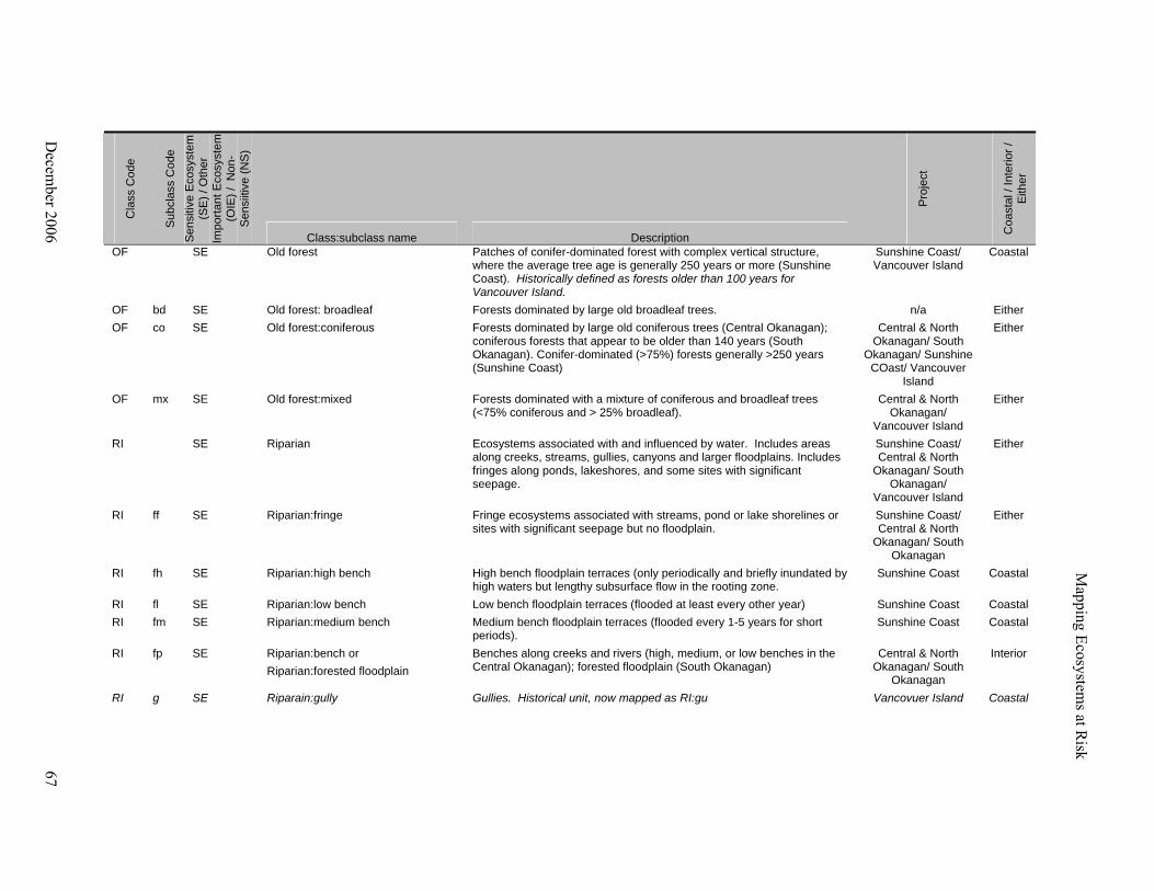
M
apping Ecosystems at R
isk
Decem
ber 2006
67
Cla
ss C
ode
Sub
clas
s C
ode
Sen
sitiv
e E
cosy
stem
(S
E) /
Oth
er
Impo
rtant
Eco
syst
em
(OIE
) / N
on-
Sen
siiti
ve (N
S)
Class:subclass name Description
Pro
ject
Coa
stal
/ In
terio
r /
Eith
er
OF SE Old forest Patches of conifer-dominated forest with complex vertical structure, where the average tree age is generally 250 years or more (Sunshine Coast). Historically defined as forests older than 100 years for Vancouver Island.
Sunshine Coast/ Vancouver Island
Coastal
OF bd SE Old forest: broadleaf Forests dominated by large old broadleaf trees. n/a Either OF co SE Old forest:coniferous Forests dominated by large old coniferous trees (Central Okanagan);
coniferous forests that appear to be older than 140 years (South Okanagan). Conifer-dominated (>75%) forests generally >250 years (Sunshine Coast)
Central & North Okanagan/ South
Okanagan/ Sunshine COast/ Vancouver
Island
Either
OF mx SE Old forest:mixed Forests dominated with a mixture of coniferous and broadleaf trees (<75% coniferous and > 25% broadleaf).
Central & North Okanagan/
Vancouver Island
Either
RI SE Riparian Ecosystems associated with and influenced by water. Includes areas along creeks, streams, gullies, canyons and larger floodplains. Includes fringes along ponds, lakeshores, and some sites with significant seepage.
Sunshine Coast/ Central & North
Okanagan/ South Okanagan/
Vancouver Island
Either
RI ff SE Riparian:fringe Fringe ecosystems associated with streams, pond or lake shorelines or sites with significant seepage but no floodplain.
Sunshine Coast/ Central & North
Okanagan/ South Okanagan
Either
RI fh SE Riparian:high bench High bench floodplain terraces (only periodically and briefly inundated by high waters but lengthy subsurface flow in the rooting zone.
Sunshine Coast Coastal
RI fl SE Riparian:low bench Low bench floodplain terraces (flooded at least every other year) Sunshine Coast Coastal RI fm SE Riparian:medium bench Medium bench floodplain terraces (flooded every 1-5 years for short
periods). Sunshine Coast Coastal
RI fp SE Riparian:bench or Benches along creeks and rivers (high, medium, or low benches in the Central Okanagan); forested floodplain (South Okanagan)
Central & North Okanagan/ South
Okanagan
Interior Riparian:forested floodplain
RI g SE Riparain:gully Gullies. Historical unit, now mapped as RI:gu Vancovuer Island Coastal

68
Decem
ber 2006
Mapping Ecosystem
s at Risk
Cla
ss C
ode
Sub
clas
s C
ode
Sen
sitiv
e E
cosy
stem
(S
E) /
Oth
er
Impo
rtant
Eco
syst
em
(OIE
) / N
on-
Sen
siiti
ve (N
S)
Class:subclass name Description
Pro
ject
Coa
stal
/ In
terio
r /
Eith
er
RI gu SE Riparian:gully Watercourse is in a steep V-shaped gully (Sunshine Coast); gullies with intermittent or permanent creeks (Central Okanagan/ South Okanagan)
Sunshine Coast/ Central & North
Okanagan/ South Okanagan
Either
RI ri SE Riparian:river Large river watercourses including gravel bars Central & North Okanagan/ South
Okanagan
Either
RI sh SE Riparian:shrub floodplain Shrub dominated floodplain or lakeshore. South Okanagan Interior SG co OIE Older Second Growth Forest:
coniferous Conifer forests 60-100 years old with <15% deciduous. Historical unit, now mapped as MF:co.
Vancovuer Island Coastal
SG mx OIE Older Second Growth Forest: mixed Older forests 60-100 years old with >15% deciduous. Historical unit, now mapped as MF:mx.
Vancovuer Island Coastal
SS Sagebrush steppe Optional class where sagebrush dominated ecosystems are separated from grasslands
South Okanagan Interior
SS ds SE Sagebrush steppe: disturbed Shrub steppe ecosystems where greater than 60% of plant cover is comprised of invasive alien species; overrides all other shrub steppe subclasses where it occurs.
South Okanagan Interior
SS ss SE Sagbrush steppe:sagebrush steppe Typical sagebrush steppe ecosystems. Optional subclass for use where it helps meet project objectives.
South Okanagan Interior
SS ss SE Sagebrush steppe Shrub steppe ecosystems on slopes <25% in fair to good condition. Variable soil depth.
South Okanagan Interior
SS st SE Grasslands:steep slope, deep soils Shrub steppe ecosystems on slopes >25%; deep soils. Optional subclass for use where it helps meet project objectives.
South Okanagan Interior
SV SE Sparsely Vegetated Areas with 5-10% cover of vascular vegetation Central & North Okanagan/ South
Okanagan/ Vancouver Island
Interior
SV cl SE Sparsely Vegetated:cliff Steep rock slopes, often near vertical, with exposed bedrock; may have <5% vegetation cover
Central & North Okanagan/ South
Okanagan/ Vancouver Island
Interior
SV gr SE Sparsely Vegetated:shallow soil Sparse grassland vegetation on very shallow soils (<20cm deep) Naramata Interior

M
apping Ecosystems at R
isk
Decem
ber 2006
69
Cla
ss C
ode
Sub
clas
s C
ode
Sen
sitiv
e E
cosy
stem
(S
E) /
Oth
er
Impo
rtant
Eco
syst
em
(OIE
) / N
on-
Sen
siiti
ve (N
S)
Class:subclass name Description
Pro
ject
Coa
stal
/ In
terio
r /
Eith
er
Central & North Okanagan SV ro SE Sparsely Vegetated:rock outcrop Rock outcrops not dominated by shrubs (was HB:ro) Interior
SV sd SE Sparsely Vegetated:coastal sand dunes
Sand dunes. Historical unit, now mapped as HB:du. Vancouver Island Coastal
SV sh SE Sparsely Vegetated:shrub Shrub dominated rock outcrop areas Central & North Okanagan/ South
Okanagan
Interior
SV sp SE Sparsely Vegetated: sand spits Coastal gravels and sand spits. Historical unit, now mapped as HB:sp. Vancouver Island Coastal SV ta SE Sparsely Vegetated:talus Areas dominated by rubbly blocks of rock (talus) Central & North
Okanagan/ South Okanagan
Interior
WD SE Woodland Dry, open stands generally with between 10 and 25% tree cover (Sunshine Coast). Open stands of Douglas-fir or ponderosa pine, often on shallow soils, 10-20% canopy cover in unaltered state (Central & North Okanagan). Historically defined as less than 50% canopy cover for Vancouver Island.
Sunshine Coast/ Central & North
Okanagan/ South Okanagan/
Vancouver Island
Either
WD bd SE Woodland:broadleaf Broadleaft (Garry oak and trembling aspen) dominated woodland stands. Historical unit, now mapped as BW
Vancouver Island Coastal
WD co SE Woodland:coniferous Conifer dominated woodland stands including open stands on shallow soils, steep warm aspects or high elevations where climate restricts tree productivity.
Sunshine Coast/ Central & North
Okanagan/ South Okanagan
Either
WD mx SE Woodland:mixed Mixed conifer and broadleaf stands. Greater than 25% coniferous and >25% broadleaf trees.
Sunshine Coast Coastal
WN SE Wetland Areas characterized by daily, seasonal or year-round water at or above the surface.
Sunshine Coast/ Central & North
Okanagan/ South Okanagan/
Vancouver Island
Either
WN bg SE Wetland:bog Bog. Nutrient-poor peat wetlands on organic (sphagnum) soils; water source from precipitation.
Sunshine Coast / Vancouver Island
Either
WN fn SE Wetland:fen Fen. Groundwater-fed peat (sedge) wetlands; primary water source is groundwater or runoff.
Sunshine Coast/ South Okanagan/ Vancouver Island
Either

Mapping Ecosystem
s at Risk
Interior
Cla
ss C
ode
Sub
clas
s C
ode
Sen
sitiv
e E
cosy
stem
(S
E) /
Oth
er
Impo
rtant
Eco
syst
em
(OIE
) / N
on-
Sen
siiti
ve (N
S)
Class:subclass name Description
Pro
ject
Coa
stal
/ In
terio
r /
Eith
er
WN ms SE Wetland:marsh Marsh. Graminoid or forb-dominated freshwater, estuarine or saline nutrient-rich wetlands that are permanently or seasonally inundated.
Sunshine Coast/ Central & North
Okanagan/ South Okanagan/
Vancouver Island
Either
WN sc SE Wetland:shrub carr Shrub carr. Shrub-dominated ecosystems with moist soils on frost-prone depressions.
n/a
WN sp SE Wetland:swamp Swamp. Shrub or tree-dominated wetlands with temporary shallow flooding and significant above or below ground water flow
Sunshine Coast/ Central & North
Okanagan/ South Okanagan/
Vancouver Island
Either
WN sw SE Wetland:shallow water Shallow water. Permanently flooded, less than 2m deep mid-summer and less than 10% cover of emergent vegetation.
Sunshine Coast/ Central & North
Okanagan/ South Okanagan/
Vancouver Island
Either
WN wm SE Wetland:wet meadow Wet meadow. Briefly inundated, graminoid-dominated meadows. Sunshine Coast/ Central & North
Okanagan/ South Okanagan/
Vancouver Island
Either
70
Decem
ber 2006

Mapping Ecosystems at Risk
Appendix E: Data Dictionary The data dictionary indicates the order, name, and type and length of fields to include in the SEI non-spatial databases. Include all fields in the order indicated regardless of whether they are populated with values.
Table 18 – Sensitive Ecosystems mapping project meta-data.
Req
uire
d
LEN
GTH
Form Name (Name in English)
CA
SE
TYPE
FIELD NAME DESCRIPTION
BAPID Business Area Project ID Y A unique identifier assigned by Resource Information Branch, MSRM to each mapping project, for tracking/management of all files in that project.
5 C
Proj_name The common name of the project - usually a well-known local place or feature.
Project name 100
C M Y
Geog_loc The geographic location of the mapping project. This is a gazetted name taken from published map; for example, a town, lake, or watershed.
Geographic location 254
C M Y
Map_scale The source scale on which the ecosystem polygons were captured. Ex. 20000 not 1:20000
Map scale 8 C M Y
Compl_date The date on which the project was completed, Format: yyyy-mm-dd
Project Completion Date 10 D Y
Surv_date Date(s) of field inventory(s) Date surveyed 254
C M Y
ESIL The sampling intensity characterized according to percentage of polygons that have been field inspected or density of inspections by area. Coding must follow Table 6-3 in the Standard for Terrestrial Ecosystem Mapping in British Columbia.
Ecosystem Survey Intensity Level
1 C Y
Accuracy A number from 1-6 based level of accuracy assessment used. See Protocol for quality assurance and accuracy assessment of ecosystem maps (Meidinger 2003).
Accuracy Assessment 1 C Y
Mapsh_nbr The mapsheet number that the ecosystem mapping personnel worked on. Leading zero required for mapsheets not starting with 1, left justified with no decimal separator.
Mapsheet number 9 C U Y
Org_name The public or private-sector organization responsible for the mapping project.
Consultant/ Organization 80 C M Y
Proj_Sup The registered professional responsible for project signoff.
Project Supervisor 80 C M Y
Eco_map The person who originally captured the Sensitive Ecosystem Mapping data or the person who developed the ratings tables (logic) to theme SE from other ecosystem data.
Ecosystem mapping personnel or modeller
80 C M Y
December 2006 71

Mapping Ecosystems at Risk
Req
uire
d
LEN
GTH
Form Name (Name in English)
CA
SE
TYPE
FIELD NAME DESCRIPTION
Dig_cap The individual or organization responsible for digital data capture. This is a required field if the SE data is mapped traditionally from stereo imagery. If modelled from TEM or other mapping see the project meta-data for that project to determine who captured the spatial data.
Digital data capture 125
C M N*
GIS_Sup The public or private-sector individual responsible for sign off on the spatial digital data. This is a required field if the SE data is mapped traditionally from stereo imagery. If modelled from TEM or other mapping see the project meta-data for that project to determine who captured the spatial data.
GIS Supervisor 80 C M N*
Rec_Name The person(s) who entered the project and polygon attribute data into a database.
Recorder Name 254
C M Y
Client The client (public or private organization) for whom the project was completed.
Project Client 80 C M Y
Trim_nbr The version of TRIM mapsheets used for Ecosystem mapping. 1 for TRIM version 1; 2 for TRIM version 2; 3 for a composite of TRIM version 1 and 2; 4 for quad system under TRIM version 1; 5 for quad system under TRIM version 2; or 6 for a quad composite of TRIM version 1 and 2. See "Map Number Recording Conventions" Table in TEM Technical Standard for quad system description.
TRIM version 1 C M Y
Pho_type Indicate whether air photo is digital or analog and in color or black & white. Enter: 1 - colour; 2 - black and white; 3 - digital colour; 4 - digital black and white; 5 - orthophoto; 6 - landsat 7 - other
Image type 1 C Y
Pho_sc Scale of air photos/images used for polygon delineation and pre-typing. For example, 20000 represents 1:20000.
Image scale 8 C Y
Pho_yr Year of air photo(s) or images (yyyy) used for polygon delineation and pre-typing. In the case where several vintages of air photos/images were used, the year applicable to the majority.
Image Year 4 C Y
Pack_nbr Version of manuals used for ecosystem mapping. As codes have changed the version of manuals used must be indicated to accompany validation routines.
Version of package used 1 C Y
Ter_map The licensed professional who has done the terrain mapping (polygon delineation and pre-typing/typing). Where there is more than one mapping personnel on a project, this is the name of the project leader.
Terrain Mapping personnel
80 C M N*
TSIL The extent to which the terrain mapping for the current project has been checked on the ground. See Table: Terrain Survey Intensity Level.
Terrain Survey Intensity Level
1 C N*
72 December 2006

Mapping Ecosystems at Risk
Req
uire
d
LEN
GTH
Form Name (Name in English)
CA
SE
TYPE
FIELD NAME DESCRIPTION
Stbcls_Tp The classification system used to classify slope stability for the current project. Indicate only one of the following with an (R) Recon, (D) Detailed, or (E) Es.
Stability. Classification Type
1 C N
Proj_com This field may be used to record any pertinent information regarding the project. Use referenced classifications which are well defined and understood in the science, or provide thorough definitions for the user.
Project comments 254
C M N
December 2006 73

Mapping Ecosystems at Risk
Table 19 – Polygon attributes for Sensitive Ecosystems mapping.
FIELD NAME DESCRIPTION Form Name (Name in English)
LEN
GTH
TYPE
CA
SE
Req
uire
d
Proj_Name Project Name Y
ECP_tag Unique polygon identifier to relate spatial to nonspatial files; this number appears on the map
Ecosystem Polygon Identification (tag)
10 C U Y
Mapsh_Nbr The Mapsheet Number of the map with the largest area of the polygon falling within it.
Mapsheet Number 9 C U Y
Source Source of the data used to determine ecological polygon units. Record the most thorough inspection type here. Record any additional source information in the Poly_com field. See Section 6.3.3 in the Standard for Terrestrial Ecosystem Mapping in British Columbia, (Resources Inventory Committee 1998b).
Data source 1 C U Y
Eco_Sec A component of the hierarchical Ecoregion Classification System of British Columbia which describes areas of major physiographical and minor macroclimatic or oceanographic variation. (Demarchi 1996).
Ecosection 3 C U Y
BGC_Zone A first-rank unit in the hierarchical BGC system of the MoF. Coding must follow the Field Manual for Describing Terrestrial Ecosystems (BC Ministry of Environment, Lands, and Parks and BC Ministry of Forests 1998).
BGC Zone 4 C U Y
BGC_Subzon A second-rank unit in the BGC system occurring within particular zones. Coding must follow the Field Manual for Describing Terrestrial Ecosystems (BC Ministry of Environment, Lands, and Parks and BC Ministry of Forests 1998).
BGC Subzone 3 C L Y
BGC_Vrt A third-rank unit (BEC variant) in the BGC unit within particular zones. Coding must follow the Field Manual for Describing Terrestrial Ecosystems,(BC Ministry of Environment, Lands, and Parks and BC Ministry of Forests 1998).
BGC Variant 1 C N
BGC_Phase A fourth-rank unit (BGC phase) in the BGC system occurring within specific variants, subzones, and zones. Coding must follow the Field Manual for Describing Terrestrial Ecosystems (BC Ministry of Environment, Lands, and Parks and BC Ministry of Forests 1998).
BGC Phase 1 C L N
Poly_Loc General description of polygon location. Where possible use a gazetted name from published maps; may be a town watershed, lake, etc.
Geographic Location 50 C M N
Flight_lin the official flight line I.e. BCC94041 Flightline number 16
Air_ph Air photo number - do not include full flight line identifier with the photo number
Air Photo number 3 C M N
Photo_poly Original polygon number on the air photo Air Photo Polygon number 2 C N
Sdec_1 The proportion of the polygon covered by Component 1, in deciles
Ecosystem Decile 1 2 N Y
SECl_1 Sensitive Ecosystem Class - component 1 Sensitive Ecosystem Class, component 1
2 C U Y
74 December 2006
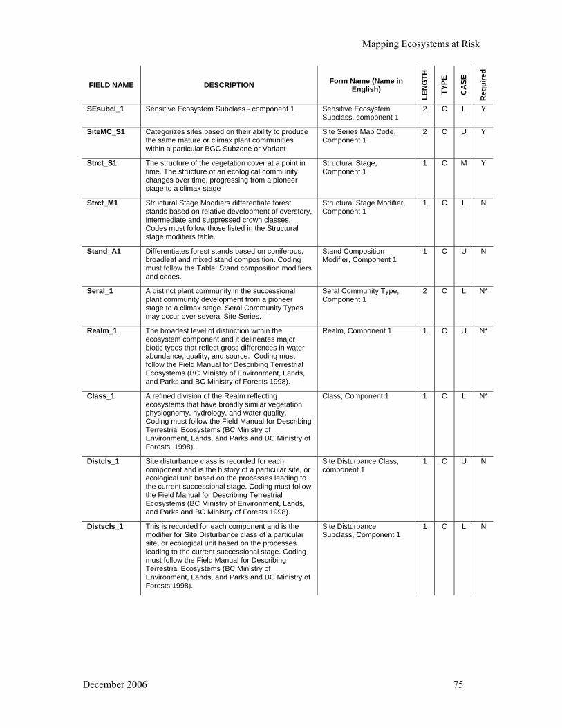
Mapping Ecosystems at Risk
FIELD NAME DESCRIPTION Form Name (Name in English)
LEN
GTH
TYPE
CA
SE
Req
uire
d
SEsubcl_1 Sensitive Ecosystem Subclass - component 1 Sensitive Ecosystem Subclass, component 1
2 C L Y
SiteMC_S1 Categorizes sites based on their ability to produce the same mature or climax plant communities within a particular BGC Subzone or Variant
Site Series Map Code, Component 1
2 C U Y
Strct_S1 The structure of the vegetation cover at a point in time. The structure of an ecological community changes over time, progressing from a pioneer stage to a climax stage
Structural Stage, Component 1
1 C M Y
Strct_M1 Structural Stage Modifiers differentiate forest stands based on relative development of overstory, intermediate and suppressed crown classes. Codes must follow those listed in the Structural stage modifiers table.
Structural Stage Modifier, Component 1
1 C L N
Stand_A1 Differentiates forest stands based on coniferous, broadleaf and mixed stand composition. Coding must follow the Table: Stand composition modifiers and codes.
Stand Composition Modifier, Component 1
1 C U N
Seral_1 A distinct plant community in the successional plant community development from a pioneer stage to a climax stage. Seral Community Types may occur over several Site Series.
Seral Community Type, Component 1
2 C L N*
Realm_1 The broadest level of distinction within the ecosystem component and it delineates major biotic types that reflect gross differences in water abundance, quality, and source. Coding must follow the Field Manual for Describing Terrestrial Ecosystems (BC Ministry of Environment, Lands, and Parks and BC Ministry of Forests 1998).
Realm, Component 1 1 C U N*
Class_1 A refined division of the Realm reflecting ecosystems that have broadly similar vegetation physiognomy, hydrology, and water quality. Coding must follow the Field Manual for Describing Terrestrial Ecosystems (BC Ministry of Environment, Lands, and Parks and BC Ministry of Forests 1998).
Class, Component 1 1 C L N*
Distcls_1 Site disturbance class is recorded for each component and is the history of a particular site, or ecological unit based on the processes leading to the current successional stage. Coding must follow the Field Manual for Describing Terrestrial Ecosystems (BC Ministry of Environment, Lands, and Parks and BC Ministry of Forests 1998).
Site Disturbance Class, component 1
1 C U N
Distscls_1 This is recorded for each component and is the modifier for Site Disturbance class of a particular site, or ecological unit based on the processes leading to the current successional stage. Coding must follow the Field Manual for Describing Terrestrial Ecosystems (BC Ministry of Environment, Lands, and Parks and BC Ministry of Forests 1998).
Site Disturbance Subclass, Component 1
1 C L N
December 2006 75

Mapping Ecosystems at Risk
FIELD NAME DESCRIPTION Form Name (Name in English)
LEN
GTH
TYPE
CA
SE
Req
uire
d
Dissscls_1 This is recorded for each component and is the modifier for Site Disturbance class of a particular site, or ecological unit based on the processes leading to the current successional stage. Coding must follow the Field Manual for Describing Terrestrial Ecosystems (BC Ministry of Environment, Lands, and Parks and BC Ministry of Forests 1998).
Site Disturbance Sub-subclass, Component 1
2 C L N
Cond_1 A representation of the condition of the ecosystem unit - considers size, species diversity, disturbance and landscape fragmentation.
Condition, Component 1 1 C U N
Viab_1 A numeric representation of how viable the ecosystem unit is - considers condition, size and defensibility parameters
Viability, Component 1 1 C N
Drain_1a A letter representing the dominant soil drainage class for the first ecosystem component
1st Soil drainage class, Component 1
1 C U N
Drain_sep1 A symbol used to indicate the proportion of the two drainage classes found in the component, or to indicate the presence or absence of intermediate drainage classes. See Terrain Standard Drainage Separator Codes Table.
Drainage class separator, component 1
1 C N
Drain_1b A letter representing the secondary soil drainage class for the first ecosystem component
2nd Soil drainage class, Component 1
1 C U N
Tree_C1 The percent of ground area covered by the vertically projected crowns of the tree cover.
Tree Crown Closure, Component 1
Shrub_C1 The percent of ground area covered by the vertically projected crowns of the shrub cover. Shrub crown closure is usually estimated for shrub- or herb-dominated components, not for forest-dominated components. Shrub crown closure is useful for determining wildlife uses.
Shrub Crown Closure, Component 1
Sdec_2 Ecosystem Decile, Component 2 Ecosystem Decile 2 1 N Y
SECl_2 Sensitive Ecosystem Class - Component 2 Sensitive Ecosystem Class, component 2
2 C U N
SEsubcl_2 Sensitive Ecosystem Subclass - Component 2 Sensitive Ecosystem Subclass, component 2
2 C L N
SiteMC_S2 Site Series Map Code, Component 2 Site Series Map Code, Component 2
2 C U N
Strct_S2 Structural Stage, Component 2 Structural Stage, Component 2
2 C M N
Strct_M2 Structural Stage Modifiers differentiate forest stands based on relative development of overstory, intermediate and suppressed crown classes. Codes must follow those listed in the Structural stage modifiers table.
Structural Stage Modifier, Component 2
1 C L N
Stand_A2 Differentiates forest stands based on coniferous, broadleaf and mixed stand composition. Coding must follow the Table: Stand composition modifiers and codes.
Stand Composition Modifier, Component 2
1 C U N
Seral_2 Seral Community Type, Component 2 Seral Community Type, Component 2
2 C L N*
Realm_2 Realm, Component 2 Realm, Component 2 1 C U N*
Class_2 Class, Component 2 Class, Component 2 1 C L N
76 December 2006

Mapping Ecosystems at Risk
FIELD NAME DESCRIPTION Form Name (Name in English)
LEN
GTH
TYPE
CA
SE
Req
uire
d
Distcls_2 Site Disturbance Class, Component 2 Site Disturbance Class, component 2
1 C U N
Distscls_2 Site Disturbance Subclass, Component 2 Site Disturbance Subclass, Component 2
1 C L N
Dissscls_2 Site Disturbance Sub-subclass, Component 2 Site Disturbance Sub-subclass, Component 2
2 C L N
Cond_2 A representation of the condition of the ecosystem unit - considers size, species diversity, disturbance and landscape fragmentation.
Condition, Component 2 1 N U N
Viab_2 A numeric representation of how viable the ecosystem unit is - considers condition and defensibility parameters
Viability, Component 2 1 C N
Drain_2a A letter representing the dominant soil drainage class for the second ecosystem component
1st Soil drainage class, Component 2
1 C U N
Drain_sep2 A symbol used to indicate the proportion of the two drainage classes found in the component, or to indicate the presence or absence of intermediate drainage classes. See Terrain Standard Drainage Separator Codes Table.
Drainage class separator, component 2
1 C N
Drain_2b A letter representing the secondary soil drainage class for the second ecosystem component
2nd Soil drainage class, Component 2
1 C U N
Tree_C2 The percent of ground area covered by the vertically projected crowns of the tree cover.
Tree Crown Closure, Component 2
Shrub_C2 The percent of ground area covered by the vertically projected crowns of the shrub cover. Shrub crown closure is usually estimated for shrub- or herb-dominated components, not for forest-dominated components. Shrub crown closure is useful for determining wildlife uses.
Shrub Crown Closure, Component 2
Sdec_3 Ecosystem Decile, Component 3 Ecosystem Decile 3 1 N Y
SECl_3 Sensitive ecosystem class - component 3 Sensitive Ecosystem Class, component 3
2 C U N
SEsubcl_3 SEI Subclass Component 3 Sensitive Ecosystem Subclass, component 3
2 C L N
SiteMC_S3 Site Series Map Code, Component 3 Site Series Map Code, Component 3
2 C U N
Strct_S3 Structural Stage, Component 3 Structural Stage, Component 3
2 C M N
Strct_M3 Structural Stage Modifiers differentiate forest stands based on relative development of overstory, intermediate and suppressed crown classes. Codes must follow those listed in the Structural stage modifiers table.
Structural Stage Modifier, Component 3
1 C L N
Stand_A3 Differentiates forest stands based on coniferous, broadleaf and mixed stand composition. Coding must follow the Table: Stand composition modifiers and codes.
Stand Composition Modifier, Component 3
1 C U N
Seral_3 Seral Community Type, Component 3 Seral Community Type, Component 3
2 C L N*
Realm_3 Realm, Component 3 Realm, Component 3 1 C U N*
Class_3 Class, Component 3 Class, Component 3 1 C L N*
December 2006 77

Mapping Ecosystems at Risk
FIELD NAME DESCRIPTION Form Name (Name in English)
LEN
GTH
TYPE
CA
SE
Req
uire
d
Distcls_3 Site Disturbance Class, Component 3 Site Disturbance Class, component 3
1 C U N
Distscls_3 Site Disturbance Subclass, Component 3 Site Disturbance Subclass, Component 3
1 C L N
Dissscls_3 Site Disturbance Sub-subclass, Component 3 Site Disturbance Sub-subclass, Component 3
2 C L N
Cond_3 A representation of the condition of the ecosystem unit - considers size, species diversity, disturbance and landscape fragmentation.
Condition, Component 3 1 N U N
Viab_3 A numeric representation of how viable the ecosystem unit is - considers condition, size and defensibility parameters
Viability, Component 3 1 C N
Drain_3a A letter representing the dominant soil drainage class for the third ecosystem component
1st Soil drainage class, Component 3
1 C U N
Drain_sep3 A symbol used to indicate the proportion of the two drainage classes found in the component, or to indicate the presence or absence of intermediate drainage classes. See Terrain Standard Drainage Separator Codes Table.
Drainage class separator, component 3
1 C N
Drain_3b A letter representing the secondary soil drainage class for the third ecosystem component
2nd Soil drainage class, Component 3
1 C U N
Tree_C3 The percent of ground area covered by the vertically projected crowns of the tree cover.
Tree Crown Closure, Component 3
Shrub_C3 The percent of ground area covered by the vertically projected crowns of the shrub cover. Shrub crown closure is usually estimated for shrub- or herb-dominated components, not for forest-dominated components. Shrub crown closure is useful for determining wildlife uses.
Shrub Crown Closure, Component 3
Microsite Ecosystem representing less than 10% of polygon Microsite 2 C U N
Frag Landscape context of polygon; degree of fragmentation of surrounding landscape
Fragmentation 2 C U N
Plot_no Field plot number Plot Number 10 C M N
poly_com This field holds any pertinent information regarding the polygon. Use referenced classifications which are well defined and understood in the science, or provide thorough definitions for the user. Use this field to record addition information regarding disturbance or condition. Record information about ecosystem units representing less than 10% of the polygon using SE class, subclass, site series map code, and structural stage. For example, MF:co HK/6.
Polygon Comments 254
C M N
78 December 2006

Mapping Ecosystems at Risk
December 2006 79
Appendix F: Example Vegetation Tables for SEI Reports Table 20 - Example riparian vegetation table for the Central Okanagan SEI28 (from Iverson and Cadrin 2003). Bench Gully Fringe Trees
black cottonwood ** ** Populus balsamifera ssp. trichocarpa Douglas-fir ** ** ** Pseudotsuga menziesii paper birch ** ** ** Betula papyrifera
western redcedar ** ** Thuja plicata trembling aspen ** ** ** Populus tremuloides
Shrubs common snowberry ** ** ** Symphoricarpos albus red-osier dogwood ** ** ** Cornus stolonifera
thimbleberry * ** Rubus parviflorus Douglas maple ** ** ** Acer glabrum
water birch ** ** ** Betula occidentalis Nootka rose ** ** ** Rosa nutkana
mock orange ** ** Philadelphus lewisii black gooseberry ** Ribes lacustre
Grasses blue wildrye * * ** Elymus glaucus
Forbs Star-flowered false Solomon’s seal ** ** ** Maianthemum racemosum
Horsetail ** * Equisetum spp.
Table 21 - Example wetland vegetation table for the Central Okanagan SEI29 (from Iverson and Cadrin 2003). Marsh Swamp Shallow
Water
Shrubs plane-leaved willow ** Salix planifolia
red-osier dogwood ** Cornus stolonifera Grasses, Sedges & Rushes
sedges ** * Carex spp. rushes ** Schoenoplectus spp.
Forbs cattail ** Typhus latifolia
duckweed ** ** Lemna minor water smartweed * ** Polygonum amphibium
pondweeds * Potamogeton spp.
28 This table broadly shows what vegetation occurred in these ecosystems. Abundance of different species is indicated by: * uncommon species, ** common species, *** abundant species. 29 As above.

80
Appendix G: Example SEI Ratings Table Below is an example of a portion of the ratings table used by the ERM tool to create a thematic SEI map from a TEM map.
Table 22. Portion of the table used to convert TEM units to SEI units for the Central Okanagan SEI. ECO_SEC BGC_ZONE BGC_SUBZON BGC_VRT BGC_PHASE SITEMC_S SITE_MA SITE_MB STRCT_S STRCT_M STAND_A SERAL HECTARES SEI_CLS SEI_SCLS SEI_FINAL
NOB IDF xh 1 AM 3 BW as BW:as NOB IDF xh 1 AM 4 B 7.022604 BW as BW:as NOB IDF xh 1 AM 5 B 8.520037 BW as BW:as NOB IDF xh 1 AM 6 B 3.117051 BW as BW:as NOB IDF xh 1 AM 7 OF bd OF:bd NOB IDF xh 1 AM g 6 M 4.267627 BW as BW:as NOB IDF xh 1 AM g 7 OF bd OF:bd NOB IDF xh 1 AM k 3 B 3.777579 BW as BW:as NOB IDF xh 1 AM k 4 BW as BW:as NOB IDF xh 1 AM k 5 B 3.375035 BW as BW:as NOB IDF xh 1 AM k 6 BW as BW:as NOB IDF xh 1 AM k 7 OF bd OF:bd NOB IDF xh 1 AO 3 0.486224 RI ff RI:ff NOB IDF xh 1 AO 4 RI ff RI:ff NOB IDF xh 1 AO 5 B 0.65855 RI ff RI:ff NOB IDF xh 1 AO 6 RI ff RI:ff NOB IDF xh 1 AO 7 RI ff RI:ff NOB IDF xh 1 AO a 3 RI fp RI:fp NOB IDF xh 1 AO a 4 RI fp RI:fp NOB IDF xh 1 AO a 5 B 0.974525 RI fp RI:fp NOB IDF xh 1 AO a 6 B 0.362808 RI fp RI:fp NOB IDF xh 1 AO a 7 RI fp RI:fp NOB IDF xh 1 AO g 3 RI gu RI:gu NOB IDF xh 1 AO g 4 RI gu RI:gu

Mapping Ecosystems at Risk
Appendix H: Example Element Occurrence Specifications Below are two generalized sample element occurrence specifications: one for south coast matrix circumesic forests and one for matrix grasslands.
Matrix South Coast Circumesic Forests Example Element Occurrence Specification30
SPECS GROUP
n/a
MINIMUM SIZE
2 ha
EO SEPARATION
SEPARATION BARRIERS
Barriers that would separate patches of these communities include large non-forested patches, a major highway, urban development, and an open body of water.
SEPARATION DISTANCE – DIFFERENT NATURAL/SEMI-NATURAL COMMUNITIES
2 km
SEPARATION DISTANCE – CULTURAL VEGETATION
0.5 km
ALTERNATE SEPARATION PROCEDURE
SEPARATION JUSTIFICATION
The separation distance for cultural vegetation is based on the suggested minimum value since little is known about limitations on forest vegetation seed dispersal. The separation distance for intervening natural or semi-natural communities seems to be a pragmatically useful distance.
FEATURE LABELS
GSPECS AUTHORSHIP
GSPECS DATE
GSPECS NOTES
30 Adapted from Chappell et al. 2004
December 2006 81
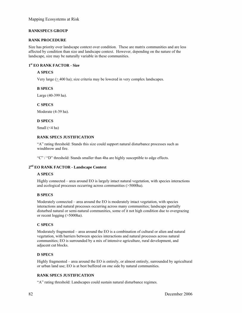
Mapping Ecosystems at Risk
RANKSPECS GROUP
RANK PROCEDURE
Size has priority over landscape context over condition. These are matrix communities and are less affected by condition than size and landscape context. However, depending on the nature of the landscape, size may be naturally variable in these communities.
1st EO RANK FACTOR - Size
A SPECS
Very large (> 400 ha); size criteria may be lowered in very complex landscapes.
B SPECS
Large (40-399 ha).
C SPECS
Moderate (4-39 ha).
D SPECS
Small (<4 ha)
RANK SPECS JUSTIFICATION
“A” rating threshold: Stands this size could support natural disturbance processes such as windthrow and fire.
“C” / “D” threshold: Stands smaller than 4ha are highly susceptible to edge effects.
2nd EO RANK FACTOR - Landscape Context
A SPECS
Highly connected – area around EO is largely intact natural vegetation, with species interactions and ecological processes occurring across communities (>5000ha).
B SPECS
Moderately connected – area around the EO is moderately intact vegetation, with species interactions and natural processes occurring across many communities; landscape partially disturbed natural or semi-natural communities, some of it not high condition due to overgrazing or recent logging (>5000ha).
C SPECS
Moderately fragmented – area around the EO is a combination of cultural or alien and natural vegetation, with barriers between species interactions and natural processes across natural communities; EO is surrounded by a mix of intensive agriculture, rural development, and adjacent cut blocks.
D SPECS
Highly fragmented – area around the EO is entirely, or almost entirely, surrounded by agricultural or urban land use; EO is at best buffered on one side by natural communities.
RANK SPECS JUSTIFICATION
“A” rating threshold: Landscapes could sustain natural disturbance regimes.
82 December 2006

Mapping Ecosystems at Risk
“C” / “D” threshold: Processes such as natural disturbances are essentially irretrievable.
3rd EO RANK FACTOR - Condition
A SPECS a. Overstory structure intact (unlogged old growth) and dominated by large, old, trees with
multilayered structure; either >140 years or >250 years depending on the biogeoclimatic subzone.
b. Vegetation is composed of native species. c. Minimal understory disturbance.
B SPECS a. Overstory structure intact, perhaps with some selective logging. Stand age is >80 years. b. If thinning has occurred, there is little evidence of disruption of understory vegetation. c. Vegetation is predominantly native species with no invasive alien species.
C SPECS a. Logged with only small diameter trees remaining and disturbance to understory vegetation.
Stand age may range from 40-80 years old. b. Vegetation is mostly native species with some alien species and < 5% invasive alien
species.
D SPECS a. Logged, perhaps clearcut, less than 40 years old. b. Ground disturbed and vegetation is disrupted. c. Vegetation has invasive alien species.
RANK SPECS JUSTIFICATION
“A” ranking threshold: Most forests begin to take on old growth characteristics earlier than 140 (>80) or 250 (>120) years.
“C”/ “D” threshold: Native understory vegetation is severely altered and species composition and structure recovery would take more than 100 years.
GRANKSPECS AUTHORSHIP
GRANKSPECS DATE
GRANKSPECS NOTES
Matrix Grassland Element Occurrence Specification SPECS GROUP
MINIMUM SIZE
2 ha
EO SEPARATION
SEPARATION BARRIERS
Barriers that would separate patches of this community include large forest patches, a major highway, urban development, and an open body of water.
December 2006 83

Mapping Ecosystems at Risk
SEPARATION DISTANCE – DIFFERENT NATURAL/SEMI-NATURAL COMMUNITIES
2 km
SEPARATION DISTANCE – CULTURAL VEGETATION
0.5 km
ALTERNATE SEPARATION PROCEDURE
SEPARATION JUSTIFICATION
The separation distance for cultural vegetation is based on the suggested minimum value, since little is known about limitations on grassland seed dispersal. The separation distance for intervening natural or semi-natural communities seems to be a pragmatically useful distance.
FEATURE LABELS
GSPECS AUTHORSHIP
GSPECS DATE
GSPECS NOTES
RANKSPECS GROUP
RANK PROCEDURE
Size has priority over condition and condition is equivalent to landscape context. Although this is usually a matrix community where landscape condition has priority over condition, increased priority for grassland condition is relevant in highly disturbed landscapes as it is a significant determinant of long-term persistence of the EO. Similarly, landscape context has an influence over the possibility of invasion of alien plants and the long-term persistence of the EO. In extreme situations, condition and landscape may both have priority over size.
1st EO RANK FACTOR - Condition
A SPECS a. Ecological community composition is climax. b. Vegetation is composed primarily of native species (<5% non-invasive alien species). c. Microbiotic crust is intact and well-developed. d. There is no evidence of grazing by domestic livestock. e. There is evidence that natural fire regimes have not been significantly altered. There is
no tree encroachment.
B SPECS a. Ecological community composition is late seral. b. Vegetation is predominantly native species with up to 20% invasive alien species. c. Microbiotic crust covers greater than 80% of the soil surface between vascular plants. d. There is low to moderate evidence of grazing by domestic livestock. e. There is minimal evidence that natural fire regimes have been altered. There may be a
few trees encroaching.
C SPECS a. Ecological community composition is early or mid-seral. b. Vegetation is mostly native species with up to 60% invasive alien species.
84 December 2006

Mapping Ecosystems at Risk
c. Microbiotic crust is present in patches but is not continuous and may be dominated by earlier seral scale and crust lichens.
d. There is moderate to high evidence of grazing by domestic livestock. e. There is some evidence that natural fire regimes have been altered. There are trees
encroaching on the site but grassland vegetation dominates.
D SPECS a. Ecological community composition is early-seral. b. Vegetation is more than 60% invasive alien species. c. Microbiotic crust is largely absent. d. There is high evidence of over-grazing by domestic livestock. e. There is evidence that natural fire regimes have been substantially altered.
Encroaching trees may dominate the site.
RANK SPECS JUSTIFICATION
“A” ranking threshold: the EO is not likely to be overtaken by alien plants or encroaching trees.
“C”/ “D” threshold: Native vegetation composition is severely altered and unlikely to replace alien species. Recovery is unlikely without invasive alien plant control.
2nd EO RANK FACTOR - Landscape Context
A SPECS
Highly connected – area around EO is largely intact natural vegetation, with species interactions and ecological processes occurring across communities (>1000ha).
B SPECS
Moderately connected – area around the EO has moderately intact vegetation, with species interactions and natural processes occurring across many communities; landscape partially disturbed natural or semi-natural communities, some of it not high condition due to overgrazing or recent logging (>1000ha).
C SPECS
Moderately fragmented – area around the EO is a combination of cultural or alien and natural vegetation, with barriers between species interactions and natural processes across natural communities; EO is surrounded by a mix of intensive agriculture, rural development, and adjacent timber harvesting areas.
D SPECS
Highly fragmented – area around the EO is entirely, or almost entirely, surrounded by agricultural or urban land use; EO is at best buffered on one side by natural communities.
RANK SPECS JUSTIFICATION
“A” rating threshold: Landscapes could sustain natural disturbance regimes.
“C” / “D” threshold: Processes such as natural disturbances are essentially irretrievable. The EO has a high probability of being overtaken by invasive alien plants.
3rd EO RANK FACTOR - Size
A SPECS
Very large (>200 ha; >50 ha in IDF)
December 2006 85

Mapping Ecosystems at Risk
B SPECS
Large (50-199 ha; 30-49 ha in IDF)
C SPECS
Moderate (10-49 ha; 5-29 ha in IDF)
D SPECS
Small (<10ha; <5ha in IDF)
RANK SPECS JUSTIFICATION
“A” rating threshold: Occurrences these sizes are likely to support the full local complement of species and can support natural disturbance processes such as fire.
“C” / “D” threshold: Occurrences these sizes are highly susceptible to edge effects including invasion of alien plants and tree encroachment. Communities this size may not be able to support natural disturbance processes such as fire unless the surrounding vegetation is unaltered natural vegetation.
GRANKSPECS AUTHORSHIP
GRANKSPECS DATE
GRANKSPECS NOTES
86 December 2006

Mapping Ecosystems at Risk
Appendix I: Example Separation Distance Specifications Below are examples of separation distances for matrix, large patch, small patch, and linear communities (Natureserve 2002).
Example Separation Distances for Matrix Communities Matrix circumesic forests: minimum size 2 ha. (1) substantial barriers to natural processes or species movement, including cultural vegetation (including clearcuts or tree plantations) greater than 0.5 km wide, major highways, urban development, large bodies of water; (2) a different natural community wider than 1 km if the communities do not frequently occur in a mosaic or 2 km if the communities frequently occur together in a mosaic; (3) a major break or change in the ecological land unit (e.g., topography, soils, geology).
Justification: Many of these communities occur naturally in a mosaic; minor breaks or small barriers are probably a common part of the natural distribution and variability. If the breaks are larger, barriers may exist for some species.
Example Separation Distances for Large Patch Communities Dry Douglas-fir and Douglas-fir – Arbutus woodlands, minimum size 0.4 ha (can be small patch). (1) substantial barriers to natural processes or species movement, including cultural vegetation (includes clearcuts/tree plantations) greater than .5 km wide, major highways, urban development, large bodies of water; (2) a different natural community wider than 1 km; (3) a major break or change in the ecological land unit (e.g., topography, soils, geology).
Justification: These communities are somewhat specific in the environment within which they occur, but can be intergraded with other forest communities, so separation distances are intermediate.
Example Separation Distances for Small Patch Communities Herbaceous balds & bluffs minimum size 0.05 ha. (1) substantial barriers to natural processes or species movement, including cultural vegetation greater than 0.5 km wide, major highways, urban development, large bodies of water; (2) a different natural community wider than 1 km; (3) a major break or change in the ecological land unit (e.g., topography, soils, geology).
Justification: Occurrences further away than 1 km are unlikely to have much interaction. Small patches associated with specific environments.
Intertidal Marshes: minimum size 0.05 ha. Substantial barriers to natural processes or species movement, including cultural vegetation greater than 0.25 km wide, roadways, artificial structures, urban development.
December 2006 87

Mapping Ecosystems at Risk
Justification: Intertidal marsh communities are usually intermixed. They sometimes occur as mosaics over large areas at estuaries of major rivers and other intertidal marsh communities are probably not barriers.
Oak Woodlands: minimum size 0.4 ha (can also be large patch). (1) substantial barriers to natural processes or species movement, including cultural vegetation (includes clearcuts/tree plantations) greater than 0.5 km wide, major highways, urban development, large bodies of water; (2) a different natural community wider than 1 km; (3) a major break or change in the ecological land unit (e.g., topography, soils, geology).
Justification: These are naturally patchy communities in British Columbia.
Example Separation Distances for Linear Communities Spits and dunes: minimum size 0.05 ha: (1) substantial barriers to natural processes or species movement, including cultural vegetation greater than 0.25 km wide, major roadways, artificial structures, urban development, large bodies of water, (2) a natural community from a different ecological group wider than 0.5 km.
Justification: These communities typically occur as linear bands together or as small patch mosaics and their location may shift over time. Communities within the same dune, spit, or berm system (site), are probably connected ecologically regardless of distance from nearest patch of same vegetation type.
Riparian Broadleaf: minimum size 0.05 ha (sometimes small patch) (1) substantial barriers to natural processes or species movement, including cultural vegetation or very degraded example of same community greater than 0.25 km wide, major roadways, urban development, large bodies of water, (2) different natural community wider than 1 km along a river corridor, or 0.5 km in other situations, (3) major break in topography, soils, geology, etc, especially one resulting in a hydrologic break.
Justification: Riparian forest communities are usually intermixed because of similar hydrologic requirements and topography. They are usually linear because of land conversion or topography.
88 December 2006