The long-range convergence of the energetic properties of the water

monomer in bulk water at room temperature

Stuart J. Davie, Peter I. Maxwell and Paul L. A. Popelier*

Manchester Institute of Biotechnology (MIB), 131 Princess Street, Manchester M1 7DN, Great Britain and

School of Chemistry, University of Manchester, Oxford Road, Manchester M13 9PL, Great Britain

*Corresponding Author: paul.popelier@manchester.ac.uk, +44 161 3064511

The Interacting Quantum Atoms (IQA) energy partitioning scheme has been applied to a set of liquid

water largely spherical clusters (henceforth called spheres) of up to 9 Å radius, with a maximum

cluster size of 113 molecules. This constitutes half of the commonly used 216 molecules in a typical

simulation box of liquid water box, and to our knowledge is the largest analysis of this kind ever

undertaken. As well as demonstrating the topological analysis of large systems, which has only

recently become computationally feasible, important long range properties of liquid water are

obtained. The full topological partitioning of each sphere into atomic basins is used to consider the

long-range convergence of the energetic and multipolar properties of the water molecule at the

centre of each sphere. It is found that the total molecular energy converges to its 9 Å value after 7

Å, which corresponds to approximately the first three solvation shells, while the molecular dipole

and quadrupole moments approximately converge after 5.5 Å, which corresponds to approximately

the first two solvation shells. The effect of water molecule flexibility is also considered.

Electronic supplementary information (ESI) available. See DOI:

1

1. Introduction

Despite the simple structure of a single water monomer, liquid water remains notoriously difficult to

simulate. One of the most significant simulation difficulties is the accurate modelling of the long-range

hydrogen bonding networks that water molecules form1-7. These hydrogen bonding networks are extremely

important to water’s bulk behavior. For example, they are considered responsible for the extremely long-

ranged, and unusually strong, hydrophobic interactions measured between organic non-polar molecules 8, 9.

The hydrogen bond network determines the energy and stability of a water cluster, directed by the

polarization of hydrogen bonds10, but such networks are susceptible to sub-femtosecond fluctuations in the

liquid phase11. Unfortunately, the spatial distribution of water can vary significantly between various point

charge models12-14, with further differences exhibited between multipolar electrostatic models15, 16. Such

results are not surprising considering the hydrogen bonding properties of water are known to be even

sensitive to nuclear quantum effects17, promoting modern reassessments of water model performances on

small systems18-20.

Understanding the behavior of water is instrumental in force field design, evidenced through the large

number of models listed in reviews21, 22. Further models focus on specific phenomena, including the main

features of vibrational spectra within water clusters23, dispersion-corrected modelling of liquid water[S. Yoo,

2011 #37]24, rigid water25, dissociative water potentials26, and transferable parameter sets for use with

biomolecules, inorganic surfaces and transition metals27. Understanding how a water molecule ‘views’ the

surrounding system is vital in developing improved water models.

One method of obtaining such a perspective is through Quantum Chemical Topology (QCT) 28. QCT brings

together several approaches that share the same central idea of partitioning a quantum mechanical property

density into a set of finite-volume fragments in real 3D space using the gradient. These fragments

correspond to topological atoms, each represented by an atomic basin that possesses an atomic nucleus and

a portion of the system’s electron density. Accordingly, changes in a basin’s electron density measures the

influence of perturbations from the surrounding system. Such an analysis of the ‘atomic horizon’ of a water

molecule at the centre of a water cluster was completed29, using the QCT branch called Quantum Theory of

Atoms in Molecules (QTAIM)30-33 and its atomic multipole moments34.

A second QCT method is the so-called Interacting Quantum Atoms (IQA)35 approach, which partitions the

energy of a system (molecule or assembly thereof) into a number of perfectly additive atomic energies that

collectively describe the distribution of energy within the molecule. Unlike QTAIM, IQA is defined away from

2

equilibrium, allowing it to provide useful insight into the nature of the hydrogen bond36, the nature of

hydrogen bond networks in small water clusters37,38, and the convergence of an atomic energy in

oligopeptide chains.

Here, IQA decomposed a system’s energy, , into a sum of individual atomic energies, , further

decomposed into a ‘self’ (or intra-atomic) energy, , and an interaction energy, ,

(1)

Here, A represents each individual atom, encompasses the atom’s kinetic energy, , the potential

energy between the electrons, , and potential energy between the electrons and the nucleus, .

Note that A’ always refers to all atoms except A. The interaction energy was further decomposed into a sum

of interatomic contributions,

(2)

where the interatomic nuclear and electron interactions were rearranged into two key energy components:

a classical electrostatic contribution, , and an exchange-correlation contribution, , a measure of

covalency39. Thus, AA’ should not strictly be thought of as a sum of n-body interactions, such as those in the

multi-body potentials22. Instead, AA’ represents the total interaction between A and the entire remaining

system (A’) at once. One can calculate this interaction through the pairwise sum of eqn (2) because many-

body effects are captured by the wavefunction of the total system. At no point do we consider a trimer, for

example, as a superposition of three (isolated) dimers. In other words, IQA quantities are always extracted

from the complete system’s wavefunction (i.e. trimer in that example).

Two recent strategies40, 41 have extended IQA to be compatible with the B3LYP density functional, as well

as the M06-2X functional. Without repeating the details here, the first strategy 40 is incorporated in the

AIMAll computational suite; the second41 in the program PROMOLDEN35. Finally, a further development42

has now extended IQA to Coupled Cluster with Single and Double excitations (CCSD), allowing electron

3

correlation to be investigated for small molecules. Currently, CCSD-IQA is only an option available in

PROMOLDEN.

2. Computational details

We sampled water clusters/spheres from a previous molecular dynamics simulation completed using

multipolar electrostatics (rigid body water at equilibrium geometry at MP2/aug-cc-pVTZ level of theory), at

300 K and 1 atm43 corresponding to a liquid water density of 0.996 g cm -3. The simulation cell contained 216

(=63) water molecules with Periodic Boundary Conditions (PBC). The potential possessed a Lennard-Jones

component (σ=3.14 Å and ε=0.753 kJ mol-1) to account for non-electrostatic interactions, and this was given

a cut-off of 2.5σ. The simulation time-step was set to 0.5 fs, and the simulation was run for a 20-50 ps

equilibration period. Figure 1 shows that the oxygen-oxygen radial distribution function of the simulated

water molecules is in reasonable agreement with experiment44, 45. Once equilibrated, ten water molecules

were randomly selected to act as the centre of each respective sphere. Subsequently, sets of water spheres

were built around each of the ten central water molecules in 0.5 Å steps from 1 Å up to 9 Å. Spheres of

radius R were created by including all water molecules whose oxygen atom was within R of the oxygen of the

central water molecule. From 1 Å to 2.5 Å, all ten spheres possessed just a single water molecule (the

central molecule). The value of 9 Å was selected to be the largest sphere radius for two reasons: (i) 9 Å

defines the largest sphere (in 0.5 Å steps) that can be taken from the simulation without including multiple

images of the same atoms (due to the PBC). In other words, this is the largest sphere that fits inside the

simulation box; and (ii) the cubic scaling of computation time relative to cluster radius made spheres larger

than 9 Å unviable with the currently available hardware (further discussed below). At 9 Å the spheres

possessed a minimum, maximum and mean number of molecules of 97, 113 and 102, respectively.

4

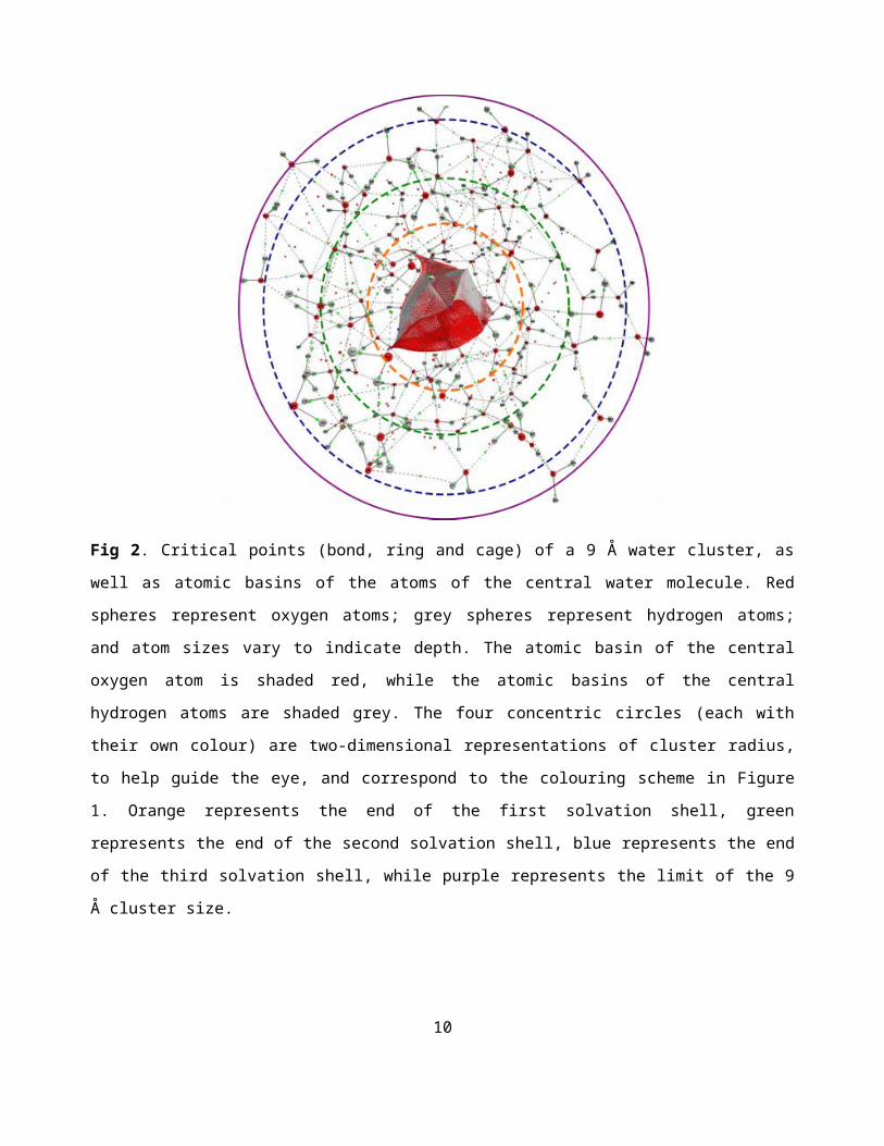
Fig. 1 Oxygen-oxygen radial distribution function for multipolar simulated water, compared to experiment 44,

45. Orange, green, and blue shading are regions of the first, second, and third solvation shells of a water

molecule in liquid water, respectively, and can be compared to the equivalently coloured radii of Fig. 2, a 9 Å

system snapshot, with solvation shells and QCT bond paths and critical points displayed.

AIMAll 46 was used to partition the water spheres into their QCT atomic basins and to calculate their IQA

energy components, using wavefunctions obtained from GAUSSIAN0947 at the B3LYP/6-311++G(d,p) level of

theory with nosymm set, and cartesian functions in use for the d and f orbitals. The B3LYP functional was

used because it is compatible with the IQA partitioning scheme40, 41, has been implemented in AIMAll, has

been shown to be capable of accurately predicting the water dipole quantitatively48, 49, and has been shown

to accurately predict the low lying energy minima of small water clusters qualitatively 48, 50-52. Although use of

relatively small basis sets have been shown to result in a shift in the dipole moment of the water monomer29,

and can result in the over-prediction of binding energies53, B3LYP/6-311++G(d,p) is popular for modelling

water50, 52, 54, 55.

AIMAll calculations were completed with the following settings: basin, outer, angular quadrature set to

auto, TWOe calculation of electron-electron potential energies switched off and the calculation of adjacent 5

interatomic surface (IAS) paths set to veryfine. Due to the complicated bond-path networks and basin

geometries (see Figure 2), several clusters possessed unusually high integration errors, L(Ω). For atoms with

an integration error of more than 0.5 kJmol-1 (oxygen) or 0.2 kJmol-1 (hydrogen), a variety of stricter

integration controls were used, with the output that obtained the lowest integration error selected for this

work. After use of stricter integration controls, the mean oxygen integration error across spheres of each

step size was lower than 0.5 kJmol-1, while the mean hydrogen integration error across spheres of each step

size was lower than 0.2 kJmol-1 for all but 4 step sizes (however the mean hydrogen integration error across

all spheres for these 4 step sizes was still less than 0.3 kJmol -1). The stricter integration controls included

manually setting the basin outer angular quadrature to skyhigh_leb or superhigh_leb, and the calculation of

adjacent interatomic surface paths set to superfine. Some of the stricter integration calculations were

completed with an updated version of AIMAll (version 15.09.12) but, apart from greater parallelization

scalability, the integration algorithms themselves were not subject to improvement between versions.

6

Fig 2. Critical points (bond, ring and cage) of a 9 Å water cluster, as well as atomic basins of the atoms of the

central water molecule. Red spheres represent oxygen atoms; grey spheres represent hydrogen atoms; and

atom sizes vary to indicate depth. The atomic basin of the central oxygen atom is shaded red, while the

atomic basins of the central hydrogen atoms are shaded grey. The four concentric circles (each with their

own colour) are two-dimensional representations of cluster radius, to help guide the eye, and correspond to

the colouring scheme in Figure 1. Orange represents the end of the first solvation shell, green represents the

end of the second solvation shell, blue represents the end of the third solvation shell, while purple

represents the limit of the 9 Å cluster size.

Calculations were run on 16-core AMD Magny-Cour nodes, possessing 2.3 GHz AMD Opteron™

Processor 6134 processors. As AIMAll allows parallelisation, the time taken in Fig. 3 assumes perfect

parallelisation, and is calculated as Time on 1 core = Time of Nc cores x Nc , for a job run using Nc cores. Figure

3 displays the times taken by the QCT program AIMAll to calculate the QCT and IQA properties of the

spheres. Only spheres with integration errors below the threshold are displayed. The high variation in

calculation times for the larger spheres is due to the large variation in complexity of the electron density’s

topology going from one sphere to another. Although spheres larger than 9 Å could be extracted from the

7

simulation by using the periodic images of adjacent cells, IQA partitioning of the energies of spheres larger

than 9 Å were difficult to obtain due to computational expense.

Fig. 3. Mean time (left), averaged over 10 spheres for each given radius, required to calculate IQA properties

and the number (right) of molecules for each sphere size. Error bars represent ±1 standard deviation.

Flexible-water spheres were created by applying energy to the system’s normal modes of vibration,

following the procedure for distortion outlined in Ref. 56, using three randomly selected rigid spheres as

‘seeds’. Although distortion frequencies were obtained at the HF level of theory, flexible-water spheres

were treated according to the previously discussed rigid spheres. Flexible-water clusters were generated

from the rigid-body clusters using the same distortion procedure in Ref. 56. For the flexible-water clusters,

frequency files were calculated at the HF level of theory but wavefunctions were calculated at the same

B3LYP/6-311++G(d,p) level of theory as the rigid-water clusters.

3. Results

3.1 Energy

Figure 4a displays the molecular energy of the central monomer in each of the 10 spheres sampled as a

function of sphere radius, as well as a curve representing the mean total molecular energy across the entire

set (in black). Figure 4b displays the convergence of the total energy by considering the absolute change in

energy between steps in sphere size, .

8

Fig. 4. (a), (c) and (e) display the total energy, self-energy, and interaction energy, respectively, of the central

water molecule in each sphere. Error bars represent total integration error for the molecule (i.e. the sum of

the three absolute atomic integration errors). Black ‘mean’ lines represent the mean across all clusters. (b),

(d) and (f) display the mean absolute difference in total energy, self-energy, and interaction energy

respectively, of the central water molecule between consecutive sphere sizes, across all spheres. Error bars

represent ±1 standard deviation.

9

Despite a 30 kJmol-1 range in the sampled 9 Å sphere molecular energies, the mean absolute change in

energy on a central water molecule at that distance, caused by a 0.5 Å increase in sphere radius, is less than

1 kJmol-1. By 7 Å, the mean molecular energy (-200,779.97 kJmol-1 in Fig. 4a) has converged to within 0.2

kJmol-1 of the 9 Å value (-200,779.81 kJmol-1), with mean energy differences approximately 1 kJmol-1 or less

between sphere sizes. Figure ESI1 shows the convergence of the exact energies (i.e. not absolute differences

in energy).

The IQA energy partitioning divides total energies into individual ‘self’ and ‘interaction’ contributions.

In eqns (1) and (2) this partitioning is carried through to atomic level. However, we can easily generate a

coarser-grained partitioning from the energies at the molecular resolution. Molecular ‘self’ and ‘interaction’

energies are obtained by simply summing each of the Nat atomic energies, where Nat is the number of atoms

in the molecule. Water’s molecular self-energy, , is then

(3)

while the molecular interaction energy is

(4)

The intramolecular interaction energies (i.e. interaction energies between the atoms of the central

molecule e.g. ) are often defined as a component of the molecular interaction energy, not of the

molecular self-energy. Our inclusion here stems from our decision to calculate by taking the difference

between and , which is computationally cheaper than calculating every pairwise interatomic

contribution. This shortcut reveals the total atomic behavior within larger system sizes at the cost of

interatomic-level insight. The inclusion of intramolecular, interatomic interaction energies in our definition

of is not expected to influence the rate of convergence of the molecular self-energies and interaction

energies, as the variation in these energies is extremely small (less than 0.05 kJmol -1, for both self- and

interaction energies, for both the oxygen and hydrogen atoms in the monomer systems).

10

Figure 4c displays the self-energy of the central water molecule as a function of sphere radius, and Fig. 4d

the mean absolute difference in self-energy across all ten spheres. Figure 4e and Fig. 4f presents analogous

information for the interaction energies. Convergence of the individual molecular self- and interaction

energies is slower than for summed molecular energy, indicating that fluctuations in one energy are largely

compensated by fluctuations in the other. There are no configurational changes to the molecules already

present in a sphere upon increasing the sphere radius (i.e. the molecules in a Nr Å sphere are identically

positioned to the equivalent molecules in a Nr+Δ Å sphere). Thus, the only change in energy of the central

water molecule is due to a redistribution of the electron density caused by the sphere’s extended hydrogen

bonding networks. The large range of energies across the different clusters is due to the significantly

different internal geometries obtained from the MD sampling, and the corresponding hydrogen networks

that this variation has caused. In other words, the exact configurations of the different clusters have resulted

in significantly different cluster energies between all of the clusters. We consider this a positive trait of the

sampled clusters: although the self- and interaction energies of a central water molecule are highly

dependent on the surrounding hydrogen bonding network, energetic convergence is reached by a practical

cluster size. For all ten spheres, molecular self-energies became less stable and molecular interaction

energies became more stable as the central water molecule gained its first solvation shell. This effect is due

to the expected positions of surrounding molecules likely to produce net stabilizing interactions (e.g. O-H…O

as opposed to O…O or H…H) in creating a hydrogen bonding network. Accordingly, all ten spheres display

configurations where the central molecule is hydrogen bonded to its first solvation shell. As such, the

interactions of the central molecule are electrostatically favourable, and the total interaction energy of the

central molecule stabilizes. Alternatively, as the first solvation shell is added, the redistribution of the

electron density around the central molecule causes the self-energy of the central molecule to increase. This

is because the most energetically favourable distribution of the electron density around a water monomer is

that which is present in an isolated monomer. By perturbing the electron density of the central molecule

through hydrogen bonding networks, the self-energy destabilises. Thus, effects that are likely to stabilize the

interaction energy are likely to destabilize the self-energy, and effects that are likely to stabilize the self-

energy are likely to destabilize the interaction energy. In other words, as the hydrogen bonding network

changes with increasing sphere radius, fluctuations in one energy will be mirrored by opposite fluctuations in

the complementary energy.

As the IQA approach to energetic partitioning allows the separation on the interaction energy into

classical and exchange-correlation components (eqn (2)), the convergence of both components can be

11

considered individually. As exchange-correlation interaction terms are expected to be shorter ranged than

classical interaction terms, a shorter ranged convergence is expected. Such a result could be useful in the

formulation of forcefields for molecular simulation, which often rely on cut-off radii to increase efficiency.

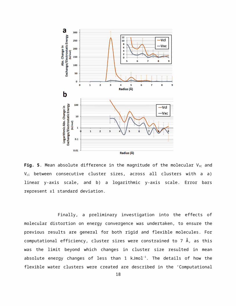
The convergence of the molecular , and energies are displayed together in Figure 5. As expected,

the convergence of the Vcl energies is slower than that of the VXC energies, while the magnitude of the

differences is significantly higher. While the mean absolute change in exchange energy is less than 1kJmol -1

from 7 Å onwards, the classical interaction energy suffers larger fluctuations. Figures ESI2-ESI9 show the

convergence of certain other individual atomic energy components, including , , and , for the

individual central oxygen and hydrogen atoms.

Fig. 5. Mean absolute difference in the magnitude of the molecular VXC and Vcl between consecutive cluster

sizes, across all clusters with a a) linear y-axis scale, and b) a logarithmic y-axis scale. Error bars represent ±1

standard deviation.

12

Finally, a preliminary investigation into the effects of molecular distortion on energy convergence was

undertaken, to ensure the previous results are general for both rigid and flexible molecules. For

computational efficiency, cluster sizes were constrained to 7 Å, as this was the limit beyond which changes in

cluster size resulted in mean absolute energy changes of less than 1 kJmol -1. The details of how the flexible

water clusters were created are described in the ‘Computational Details’ section. The absolute change in

total energy for increasing cluster sizes is displayed in Figure 6. While the energetic convergence of the

flexible water molecules is slightly different to that of the rigid molecules, the overall behavior is very similar.

Fig. 6. The mean absolute difference in total energy of the central water molecule between consecutive

sphere sizes, across all rigid (blue) and flexible (red) water spheres. Error bars represent ±1 standard

deviation.

3.2 Electrostatics

The convergence of the dipole and quadrupole moments of the central water molecule were also

considered. As water is a polar molecule, the behavior of the water dipole moment in the bulk medium has

attracted significant interest in the past, from small clusters57, 58, to clusters of up to 50 molecules29, 59, 60. As

AIMAll only calculates atomic moments, the molecular multipole moments were calculated by combining61

the corresponding atomic multipole moments. Figure 7a displays the magnitude of the dipole moment as a

function of cluster radius, while Figure 7b displays the convergence of the magnitude of the dipole moment

by considering the absolute change in energy between steps in cluster size. The dipole moment of the

13

monomer (2.16 D) turned out higher than the experimental value of 1.855 D 62, an expected result with this

Pople basis set29. Ab initio molecular dynamics on a box of 32 water molecules, using density functional

theory with local density fluctuations and gradient corrections, gave a mean dipole moment of 2.66 D63,

close to experiment64, but almost 9% higher than the value obtained here. The convergence of the

magnitude of the dipole moment to a lower value than expected may be a consequence of the selected level

of theory57. Despite a 0.5 D range in the sampled 9 Å cluster molecular energies, the mean absolute change

in the dipole moment on the central water molecule when increasing the cluster size from 8.5 Å to 9 Å is less

than 0.01 D. In fact, the mean absolute change in the magnitude of the dipole moment or any two 0.5 Å-

separated clusters equal to or larger than 6.5 Å is less than 0.02 D. Fig. ESI10 shows the convergence of the

total dipole deflection, and Figs. ESI11 and ESI12 the dipole moments of the individual atoms.

Fig. 7. (a) Total dipole moment of central water molecule for each cluster. The low dipole magnitude of

Cluster 7 is a result of the cluster’s unusually long-ranged ‘accepting’ type hydrogen bonds, and unusually

angled ‘donating’ type hydrogen bonds (b) Mean absolute difference in the magnitude of the dipole moment

between consecutive cluster sizes, across all clusters. Error bars represent ±1 standard deviation.

Figure 8a displays the magnitude of the molecular quadrupole moment as a function of cluster size, and

Figure 8b displays the mean absolute change in the magnitude of the quadrupole moment between

consecutive cluster sizes. As spherical multipole moments are used here, the magnitude of the quadrupole

moment was taken as:

14

(5)

where |Q2| is the magnitude of the quadrupole moment and {Q2,0 ,…,Q2,2 , s } are the set of spherical

quadrupole moment components. Although the mean value for the magnitude of the quadrupole moment

is similar to the monomer value, there is a range of 0.27 a.u. across the ten clusters. Relative to the total

molecular energy and molecular dipole, the molecular quadrupole converges rapidly, with a mean absolute

change in the magnitude of the quadrupole moment approximately 0.01 a.u. by 5 Å. By 5.5 Å, the magnitude

of the quadrupole moment for each cluster had converged to within 0.02 a.u. of their respective 9 Å values.

The convergence of the quadrupole moments of the individual atoms of the central water molecule is shown

in Figs. ESI13 and ESI14.

Fig. 8. (a) Magnitude of the quadrupole moment of central water molecule for each cluster. (b) Mean

absolute difference in the effective moment of the quadrupole moment between consecutive cluster sizes,

across all clusters. Error bars represent ±1 standard deviation.

4. Conclusion and Future Work

15

In conclusion, a full QCT analysis is computationally feasible for systems in excess of 100 water molecules,

about half of the 216-molecule simulation box. We obtained unprecedented insight into the long-range

convergence of a water molecule’s properties in water. By 7 Å, within the third solvation shell, mean

energetic properties of the rigid water monomer converge to within 1 kJmol -1 of the 9 Å sphere values. By

5.5 Å, about the radius of the first two solvation shells, the mean dipole moment and mean magnitude of the

quadrupole moment respectively deviated by 0.015 D and 0.005 a.u. of the corresponding 9 Å values. The

convergence of flexible water was shown to be slightly slower, although similar.

As they are, these results should provide a useful test for new water potentials to be validated against.

However, a systematic investigation into different water densities and phase states would be useful for the

formulation of more general energetic-convergence rules, which is subject of future work. Furthermore, as

application of such topological partitioning schemes are computationally feasible for large, conformationally

flexible systems, such calculations will be useful in unlocking new insights into other large systems

dominated by long range interactions, such as those involving ions.

A final comment is in order on the potential role of quantum nuclear effects17 on the hydrogen atoms.

Our work does not discuss proton transport, autoionization events or the liquid-water self-diffusion

coefficient, which are all affected by the quantum nature of hydrogen nuclei. However, a pioneering study 65

extends QTAIM beyond the Born-Oppenheimer paradigm, showing differences in the properties of atomic

basins in the presence of a nuclear wavefunction. For example, in LiH the dipole moment and electronic

charge of hydrogen is, respectively, 0.001 a.u. and 0.004 a.u. smaller in magnitude compared to those of

hydrogen in the clamped nuclei model. Hydrogen’s electronic energy is 78 kJmol -1 lower in the latter model.

Assessing such differences for water clusters belongs to future study.

Conflicts of Interest

There are no conflicts of interest to declare.

Acknowledgements

P.M. thanks the BBSRC for the award of a PhD studentship, and S.J.D. and P.L.A.P. acknowledge the EPSRC

for funding through the award of an Established Career Fellowship (grant EP/K005472).

References

1. R. L. Blumberg, H. E. Stanley, A. Geiger and P. Mausbach, J. Chem. Phys., 1984, 80, 5230-5241.

2. H.-P. Cheng, J. Phys. Chem. A, 1998, 102, 6201-6204.

16

3. R. Kumar, J. R. Schmidt and J. L. Skinner, J. Chem. Phys., 2007, 126, 204107.

4. M. Mezei and D. L. Beveridge, J. Chem. Phys., 1981, 74, 622-632.

5. D. C. Rapaport, Mol. Phys., 1983, 50, 1151-1162.

6. J. D. Smith, C. D. Cappa, K. R. Wilson, B. M. Messer, R. C. Cohen and R. J. Saykally, Science, 2004, 306,

851-853.

7. S. S. Xantheas, Chem. Phys., 2000, 258, 225-231.

8. J. Israelachvili and R. Pashley, Nature, 1982, 300, 341-342.

9. Y.-H. Tsao, D. F. Evans and H. Wennerström, Science, 1993, 262, 547-547.

10. A. M. Tokmachev, A. L. Tchougreef and R. Dronskowski, Chem. Phys. Chem., 2010, 11, 384-388.

11. A. Pietzsch, F. Hennies, P. S. Miedema, B. Kennedy, J. Schlappa, T. Schmitt, V. N. Strocov and A.

Föhlisch, Phys. Rev. Lett., 2015, 114, 088302.

12. J. Kolafa and I. V. O. Nezbeda, Mol. Phys., 2000, 98, 1505-1520.

13. I. V. O. Nezbeda and J. Kolafa, Mol. Phys., 1999, 97, 1105-1116.

14. D. J. Huggins, J. Chem. Phys., 2012, 136, 064518.

15. S. Y. Liem and P. L. A. Popelier, J. Chem. Theory Comput., 2008, 4, 353-365.

16. M. S. Shaik, M. Devereux and P. L. A. Popelier, Mol. Phys., 2008, 106, 1495-1510.

17. M. Ceriotti, J. Cuny, M. Parrinello and D. E. Manolopoulos, Proc. Natl. Acad. Sci. U.S.A., 2013, 110,

15591-15596.

18. D. C. Clary, Science, 2016, 351, 1267-1268.

19. J. O. Richardson, C. Pérez, S. Lobsiger, A. A. Reid, B. Temelso, G. C. Shields, Z. Kisiel, D. J. Wales, B. H.

Pate and S. C. Althorpe, Science, 2016, 351, 1310-1313.

20. G. R. Medders, V. Babin and F. Paesani, J. Chem. Theory Comput., 2013, 9, 1103-1114.

21. B. Guillot, J. Mol. Liq., 2002, 101, 219-260.

22. G. A. Cisneros, K. T. Wikfeldt, L. Ojamae, J. Lu, Y. Xu, H. Torabifard, A. P. Bartok, G. b. Csanyi, V.

Molinero and F. Paesani, Chem. Rev., 2016, 116, 7501.

23. G. S. Fanourgakis and S. S. Xantheas, J. Chem. Phys., 2008, 128, 074506-074501-074511.

24. S. Yoo and S. S. Xantheas, J. Chem. Phys., 2011, 134, 121105-121101-121104.

25. J. L. F. Abascal and C. Vega, J. Chem. Phys., 2005, 123, 234505-234501-234512.

26. T. S. Mahadevan and S. H. Garofalini, J. Phys. Chem. B, 2007, 111, 8919-8927.

27. T. P. Senftle, S. Hong, M. M. Islam, S. B. Kylasa, Y. Zheng, Y. K. Shin, C. Junkermeier, R. Engel-Herbert,

M. J. Janik, H. M. Aktulga, T. Verstraelen, A. Grama and A. C. T. van Duin, NPJ Comput. Mater., 2016,

2, 15011.17

28. P. L. A. Popelier, in Structure and Bonding. Intermolecular Forces and Clusters, Springer, Heidelberg,

Germany, 2005, vol. 115, pp. 1-56.

29. C. M. Handley and P. L. A. Popelier, Synth React Inorg Met Org Chem, 2008, 38, 91-100.

30. R. F. W. Bader, Atoms in molecules, Oxford Univ. Press, Great Britain, 1990.

31. P. L. A. Popelier, F. M. Aicken and S. E. O’Brien, Chemical Modelling: Applications and Theory, 2000,

1, 143.

32. P. L. A. Popelier, Atoms in Molecules. An Introduction., Pearson Education, London, Great Britain,

2000.

33. C. F. Matta and R. J. Boyd, The Quantum Theory of Atoms in Molecules. From Solid State to DNA and

Drug Design., Wiley-VCH, Weinheim, Germany, 2007.

34. P. L. A. Popelier, L. Joubert and D. S. Kosov, J. Phys. Chem. A, 2001, 105, 8254-8261.

35. M. A. Blanco, Á. M. Pendas and E. Francisco, J. Chem. Theory Comput., 2005, 1, 1096-1109.

36. Á. M. Pendas, M. A. Blanco and E. Francisco, J. Chem. Phys., 2006, 125, 184112.

37. J. M. Guevara-Vela, R. Chavez Calvillo, M. García Revilla, J. Hernandez Trujillo, O. Christiansen, E. ‐ ‐ ‐Francisco, Á. M. Pendas and T. Rocha Rinza, ‐ Chem. Eur. J, 2013, 19, 14304-14315.

38. J. M. Guevara-Vela, E. Romero-Montalvo, V. A. M. Gomez, R. Chavez-Calvillo, M. García-Revilla, E.

Francisco, Á. Martín Pendas and T. Rocha-Rinza, Phys. Chem. Chem. Phys., 2016, 18, 19557-19566.

39. M. García-Revilla, E. Francisco, P. L. Popelier and A. Martín Pendas, ChemPhysChem, 2013, 14, 1211-

1218.

40. P. Maxwell, Á. Martín Pendas and P. L. A. Popelier, Phys. Chem. Chem. Phys., 2016, 18, 20986.

41. E. Francisco, J. L. Casals-Sainz, T. Rocha-Rinza and A. M. Pendas, Theor. Chem. Acc, 2016, 135.

42. R. Chavez-Calvillo, M. García-Revilla, E. Francisco, Á. Martín Pendas and T. Rocha-Rinza,

Computational and Theoretical Chemistry, 2015, 1053, 90-95.

43. S. Y. Liem, P. L. A. Popelier and M. Leslie, Int. J. Quantum Chem., 2004, 99, 685-694.

44. A. K. Soper, Chemical Physics, 2000, 258, 121-137.

45. A. K. Soper, ISRN Physical Chemistry, 2013, Article ID 279463,.

46. T. A. Keith. AIMAll (Version 15.05.18), TK Gristmill Software, Overland Park, KS, USA, 2015.

47. M. J. Frisch, G. W. Trucks, H. B. Schlegel, G. E. Scuseria, M. A. Robb, J. R. Cheeseman, G. Scalmani, V.

Barone, B. Mennucci and G. A. Petersson, Gaussian Inc., Wallingford CT, USA, 2010.

48. M. J. Gillan, D. Alfè and A. Michaelides, J. Chem. Phys., 2016, 144, 130901.

49. A. J. Cohen and Y. Tantirungrotechai, Chem. Phys. Lett., 1999, 299, 465-472.

50. J. Kim, D. Majumdar, H. M. Lee and K. S. Kim, J. Chem. Phys., 1999, 110, 9128-9134.18

51. A. Lenz and L. Ojamae, Chem. Phys. Lett., 2006, 418, 361-367.

52. H. M. Lee, S. B. Suh, J. Y. Lee, P. Tarakeshwar and K. S. Kim, J. Chem. Phys., 2000, 112, 9759-9772.

53. V. S. Bryantsev, M. S. Diallo, A. C. T. van Duin and W. A. Goddard, J. Chem. Theory Comput., 2009, 5,

1016-1026.

54. D. J. Anick, J. Mol. STRUC-THEOCHEM, 2002, 587, 97-110.

55. G. I. Csonka, J. Mol. STRUC-THEOCHEM, 2002, 584, 1-4.

56. T. L. Fletcher, S. J. Davie and P. L. A. Popelier, J. Chem. Theory Comput., 2014, 10, 3708-3719.

57. J. K. Gregory, D. C. Clary, K. Liu, M. G. Brown and R. J. Saykally, Science, 1997, 275, 814-817.

58. K. Liu, J. D. Cruzan and R. J. Saykally, Science, 1996, 271, 929.

59. D. D. Kemp and M. S. Gordon, J. Phys. Chem. A, 2008, 112, 4885-4894.

60. I. Bako and I. Mayer, J. Phys. Chem. A, 2016, 120, 4408–4417.

61. M. Devereux and P. L. A. Popelier, J. Phys. Chem. A, 2007, 111, 1536-1544.

62. F. J. Lovas, J. Phys. Chem. Ref. Data, 1978, 7, 1445-1750.

63. K. Laasonen, M. Sprik, M. Parrinello and R. Car, J. Chem. Phys., 1993, 99, 9080-9089.

64. T. R. Dyke, K. M. Mack and J. S. Muenter, J. Chem. Phys., 1977, 66, 498-510.

65. M. Goli and S. Shahbazian, Theor. Chem. Acc., 2011, 129, 235-245.

19