Embed Size (px)
Citation preview
The StanCOG Transportation Model
Program
Documentation and Validation Report
Version 1
Adopted by the StanCOG Policy Board
March 17, 2010
Table of Contents
1. Introduction and Summary ..................................................................................... 1
1.1 Model Software ..................................................................................................................1
1.2 Transportation Conformity Rule Modeling Requirements ................................................8
1.3 Procedures to “Run the Model” ..........................................................................................9
2. Model Study Area and Zone System ................................................................... 11
2.1 Internal Zones ...................................................................................................................11
2.2 External Zones .................................................................................................................12
3. Using Cube/Voyager/ 5.1 ...................................................................................... 12
3.1 Required Resources: .........................................................................................................12
3.2 Directories ........................................................................................................................13
3.3 Model Files ......................................................................................................................13
3.4 Model Application ...........................................................................................................14
4. Modifying the Roadway Network ........................................................................ 15
4.1 Road Network Elements ..................................................................................................16
4.2 “Master” Roadway Network ...........................................................................................16
4.3 Final Combined Loaded Network ...................................................................................24
4.4 Transit Network ...............................................................................................................25
5. Land Use / External Trip Assumptions ............................................................... 25
5.1 Household Cross Classification Data ..............................................................................25
5.2 Modifying Land Use Assumptions ..................................................................................27
5.3 Using Special Generators ................................................................................................28
5.4 External Trips ..................................................................................................................29
5.5 Creating New Scenarios ..................................................................................................29
6. Mode Choice Changes ......................................................................................... 31
6.1 Transit Factors .................................................................................................................31
7. Special Assignments ........................................................................................... 33
7.1 Intersection Turn Volumes ..............................................................................................33
7.2 Select Link Analysis ........................................................................................................33
7.3 Select Zone Analysis .......................................................................................................34
8. Adjustment of Results ......................................................................................... 37
8.1 Turn Movements .............................................................................................................37
9. Reporting the Results .......................................................................................... 40
9.1 Viewing and Plotting Model Data ...................................................................................40
9.2 Posting Volumes on Loaded Networks ...........................................................................42
10. The Forecasting Process - Trip Generation ..................................................... 43
10.1 Trip Stratification ..........................................................................................................43
10.2 Trip Generation Rates (Person Trips) ...........................................................................44
10.3 Cordon or “Gateway” Trips ..........................................................................................48
10.4 Special Generators .........................................................................................................48
11. The Forecasting Process - Trip Distribution .................................................... 49
11.1 Description of Gravity Model .......................................................................................49
11.2 Zone-To-Zone Travel Times .........................................................................................49
11.3 Friction Factors ..............................................................................................................50
11.4 Adjustment Factors ........................................................................................................50
12. The Forecasting Process - Trip Assignment ................................................... 50
12.1 Traffic Assignment ........................................................................................................50
12.2 Pricing ...........................................................................................................................51
13. The Forecasting Process - Feedback Mechanisms ......................................... 52
13.1 Model Feedback Loop ...................................................................................................52
14. The Forecasting Process - Peaking Factors .................................................... 53
14.1 Time-of-Day Factors .....................................................................................................53
Appendix A – Validation ............................................................................................................55
Appendix B – Through Trips and Trips In and Out
of the Region and Percent by Purpose .............................................. 66
List of Figures
Figure 1 - Travel Demand Model Process .......................................................................................... 6
Figure 2 - Sample Master Directory ..................................................................................................... 9
Figure 3 - Travel Demand Model TAZs and Gateways ..................................................................... 12
Figure 4 - Example of Master Network Coding ................................................................................. 19
Figure 5 - Job Script Code Lines to Build Future Year Network ...................................................... 21
Figure 6 - Creating Future Year Networks ........................................................................................ 22
Figure 7 - Cube Display of Link Data ................................................................................................ 23
Figure 8 - Turn Penalty Dialog Box ................................................................................................... 25
Figure 9 - Portion of the 2030 (General Plan Year) Land Use Database ........................................... 33
Figure 10 - Sample Jobstream for Turning Volumes & Select Link Analysis ................................... 41
Figure 11 - Sample Jobstream for Select Zone Analysis ................................................................... 43
List of Tables
Table 1 TAZ Numbering Ranges ....................................................................................................... 11
Table 2 - Model Input Files ................................................................................................................ 15
Table 3 - Capacities and Speed-Delay Curves by Roadway Type ..................................................... 24
Table 4 - Loaded Network Link Attributes ........................................................................................ 28
Table 5 2006 Countywide Cross Classified Summary ...................................................................... 31
Table 6 2030 Future Year Land Use Summaries ............................................................................... 31
Table 7 2005 and 2025 (General Plan Year) Employment Summary ................................................ 32
Table 8 2025 Special Generators ....................................................................................................... 34
Table 9 - Vehicle Trips per Person Trip ............................................................................................. 37
Table 10 - Transit Service Factors ..................................................................................................... 38
Table 11 Cross Classified Single Family Trip Generation Rates ....................................................... 53
Table 12 Cross Classified Multi-Family Trip Generation Rates ........................................................ 54
Table 13 Employment Trip Generation Rates ................................................................................... 55
Table 14 Time of Day Factors ........................................................................................................... 65
1
1. INTRODUCTION AND SUMMARY
The development of the StanCOG countywide transportation model began as a multi-
jurisdictional effort in 2005-07 by the California Department of Transportation (Caltrans), the
Stanislaus County Council of Governments (StanCOG) and the City of Modesto. The purpose
was to integrate models used in the County for planning purposes using the City of Modesto
General Plan Model and the StanCOG air quality and RTP model. The integration of the models
included up to date land use and roadway network and improved model components used in the
4 step modeling process. In 2008-09, StanCOG staff continued to update key model
components of the model, designed a system to account for land use by city and community and
added network from San Joaquin and Merced counties where inter regional projects are planned.
The updated model had an important function in the development of the 2010 RTP, the 2009
CMP and the 2010 air quality conformity analysis. Model improvements will continue in 2010-
11 period to integrate origin-destination information at the gateways and implement a mode
choice component using an nested logit function from Consumer Economics.
1.1 Model Software
The StanCOG transportation model has been developed and is operable on the Cube - Voyager
(5.1) software platform. Cube is a proprietary platform developed by Citilabs. Support for these
packages and software upgrades are usually available on the Citilabs website at
www.citilabs.com. It is recommended for users to have access to Microsoft Excel to manipulate
land use and other input files. Microsoft Excel is available from the Microsoft Corporation.
Support and upgrades are available from www.microsoft.com. Microsoft Excel should be
installed with Visual Basic for Applications included in the install for full functionality.
1.1.1 Model Coverage and Traffic Analysis Zones (TAZs)
The study area for the StanCOG model covers all of Stanislaus County, including the cities and
the un-incorporated areas. It also includes the southern frontier of San Joaquin County and the
northern frontier of Merced County along the Stanislaus County borders. Stanislaus County
itself is broken up into approximately 2,500 traffic analysis zones (TAZs) including 50 gateways.
The model has capacity for 3,200 zones through zone subdivision.
1.1.2 Historical Socioeconomic Data / Land Use Inputs
The land use inputs (socioeconomic data) by TAZ include people per household, auto-ownership
and employment data segmented into five employment categories. The land use allocation
began with socioeconomic data by traffic analysis zones (TAZ) based on the 2000 Census and
the 2005 business survey by Info-USA, (2006). In 2008, StanCOG staff arranged single family
and multi family dwelling units and population data collected from the State Department of
Finance geographically using Census Tiger boundaries by city, community and the
unincorporated regions and zip code boundary in the Stanislaus region. The historical data were
collected in the year 2006. They are shown below alongside historical job data and are the basis
of the transportation model used for validation. StanCOG staff arranged job data from employer
payrolls for the Stanislaus region in year 2006. The Employment Development Department
(EDD) provided job data for retail, service, education, other ad total jobs; the other job category
include jobs in manufacturing, food processing and telecommunications and utilities. Like the
housing and population data above, the information were arranged geographically using Census
Tiger boundaries by city, community the unincorporated regions and by zip code. See table

2
above for specific historical city and community and data type. Control totals are also provided
below. In 2009-10, StanCOG staff consolidated its land use and demographic data into a
Census-Land use-Demographic Monitoring programs for the benefit of alternative programs
used by StanCOG jurisdictions.
Existing Demographics by City, Community and Unincorporated Area (2006)
P OP D U SF M F R etail Service ED U GOV o ther T o tal
C o unty C o ntro l T o tal (D .O.F . & E.D .D .)511,617 171,721 135,562 36,159 28,244 48,214 725 25,791 74,182 177,156
C o unty T o tal 511,622 171,721 135,562 36,159 28,244 48,214 16,052 10,660 74,010 177,180
B ret H arte 5,510 1,331 1,097 235 - - 14 1 161 175
B ystro m C D P 4,823 1,492 1,229 263 469 164 104 41 343 1,121
C eres city 40,723 12,641 10,200 2 ,441 1,639 1,605 1,418 587 3 ,358 8 ,607
D el R io C D P 1,247 446 368 79 - 27 - - 188 215
D enair C D P 3,679 1,238 1,020 218 44 20 109 8 120 302
East Oakdale C D P 2,927 1,099 905 194 - 17 8 - 188 213
Empire C D P 4,167 1,293 1,065 228 24 65 83 3 422 597
Grayso n C D P 1,150 309 254 54 - - - - - -
H ickman C D P 488 158 130 28 29 - 85 3 107 224
H ughso n city 6,092 1,911 1,621 290 120 6 55 10 580 771
Keyes C D P 4,884 1,567 1,291 276 50 - 131 7 343 531
M o desto city 206,993 73,501 55,948 17,553 12,519 27,833 7 ,958 6 ,154 14,152 68,616
N ewman city 10,084 3 ,092 2 ,704 388 287 187 281 49 281 1,085
Oakdale city 17,761 6 ,639 5 ,230 1,409 825 1,328 597 268 3 ,091 6 ,109
P atterso n city 19,171 5 ,414 5 ,072 342 362 534 436 329 674 2 ,334
R iverbank city 21,099 6 ,257 5 ,606 651 634 613 432 168 1,664 3 ,510
R iverdale P ark C D P 1,168 337 277 59 - - - - 140 140
Salida C D P 13,409 3 ,984 3 ,281 702 360 551 428 84 1,309 2 ,732
Shackelfo rd C D P 5,520 1,549 1,276 273 290 134 5 13 604 1,046
T urlo ck city 67,519 23,084 16,850 6 ,234 4 ,000 8 ,004 2 ,388 2 ,606 7 ,335 24,333
Waterfo rd city 8,171 2 ,448 2 ,072 376 83 41 294 29 40 486
West ley C D P 797 161 132 28 - - 3 20 - 23
West M o desto C D P 6,508 1,939 1,597 342 - - 74 - 398 472
- -
Stanislaus Uninco rpo rated 57,732 19,832 16,336 3 ,496 6 ,509 7 ,085 1,150 282 38,512 53,538
1.1.3 Future Socioeconomic Data / Land Use Inputs
Land use forecasts adopted by the StanCOG Board in December 2009 reflect the cities and
county general plan assumptions and Measure E in addition to Valleywide Blueprint
assumptions. Measure E passed in November of 2008 to limit growth in the unincorporated
county. Blueprint assumptions were adopted by the StanCOG Board that reflect relative
densities.
3
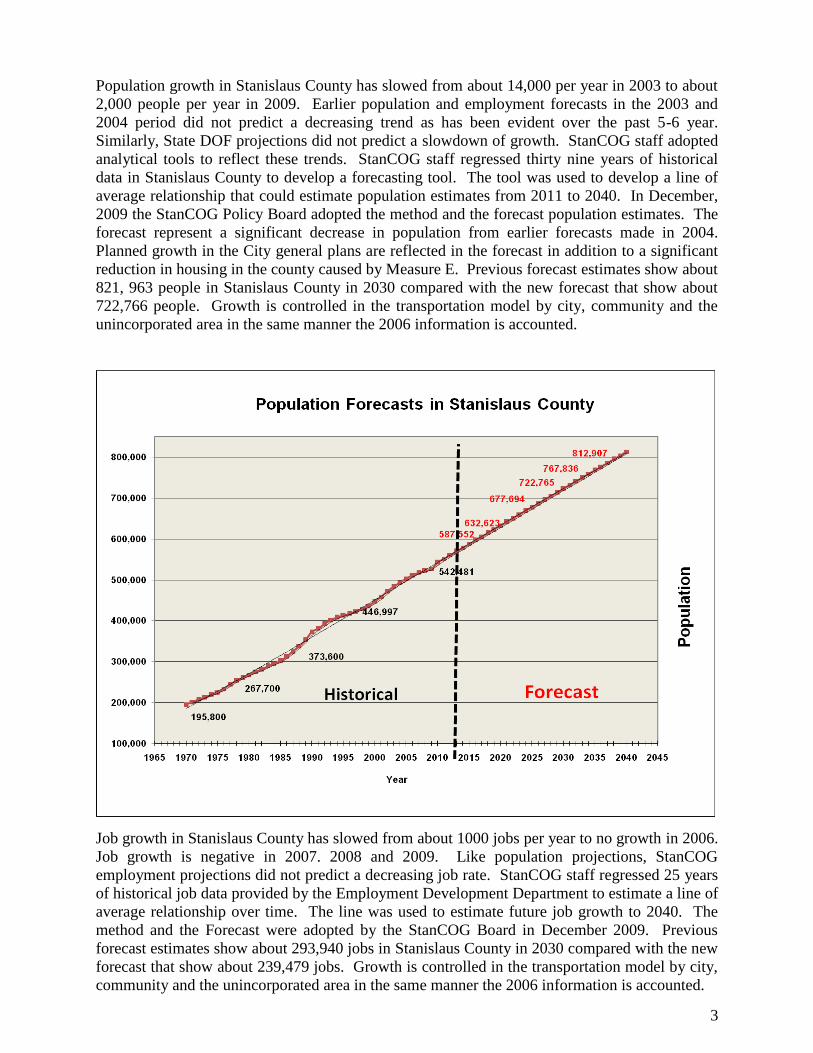
Population growth in Stanislaus County has slowed from about 14,000 per year in 2003 to about
2,000 people per year in 2009. Earlier population and employment forecasts in the 2003 and
2004 period did not predict a decreasing trend as has been evident over the past 5-6 year.
Similarly, State DOF projections did not predict a slowdown of growth. StanCOG staff adopted
analytical tools to reflect these trends. StanCOG staff regressed thirty nine years of historical
data in Stanislaus County to develop a forecasting tool. The tool was used to develop a line of
average relationship that could estimate population estimates from 2011 to 2040. In December,
2009 the StanCOG Policy Board adopted the method and the forecast population estimates. The
forecast represent a significant decrease in population from earlier forecasts made in 2004.
Planned growth in the City general plans are reflected in the forecast in addition to a significant
reduction in housing in the county caused by Measure E. Previous forecast estimates show about
821, 963 people in Stanislaus County in 2030 compared with the new forecast that show about
722,766 people. Growth is controlled in the transportation model by city, community and the
unincorporated area in the same manner the 2006 information is accounted.
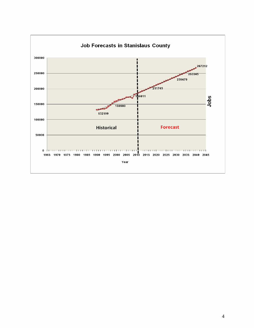
Job growth in Stanislaus County has slowed from about 1000 jobs per year to no growth in 2006.
Job growth is negative in 2007. 2008 and 2009. Like population projections, StanCOG
employment projections did not predict a decreasing job rate. StanCOG staff regressed 25 years
of historical job data provided by the Employment Development Department to estimate a line of
average relationship over time. The line was used to estimate future job growth to 2040. The
method and the Forecast were adopted by the StanCOG Board in December 2009. Previous
forecast estimates show about 293,940 jobs in Stanislaus County in 2030 compared with the new
forecast that show about 239,479 jobs. Growth is controlled in the transportation model by city,
community and the unincorporated area in the same manner the 2006 information is accounted.
4
5
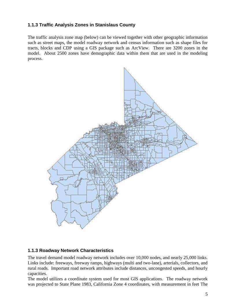
1.1.3 Traffic Analysis Zones in Stanislaus County
The traffic analysis zone map (below) can be viewed together with other geographic information
such as street maps, the model roadway network and census information such as shape files for
tracts, blocks and CDP using a GIS package such as ArcView. There are 3200 zones in the
model. About 2500 zones have demographic data within them that are used in the modeling
process.
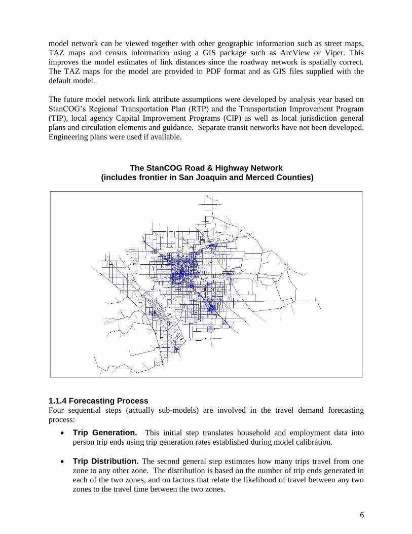
1.1.3 Roadway Network Characteristics
The travel demand model roadway network includes over 10,000 nodes, and nearly 25,000 links.
Links include: freeways, freeway ramps, highways (multi and two-lane), arterials, collectors, and
rural roads. Important road network attributes include distances, uncongested speeds, and hourly
capacities.
The model utilizes a coordinate system used for most GIS applications. The roadway network
was projected to State Plane 1983, California Zone 4 coordinates, with measurement in feet The
6
model network can be viewed together with other geographic information such as street maps,
TAZ maps and census information using a GIS package such as ArcView or Viper. This
improves the model estimates of link distances since the roadway network is spatially correct.
The TAZ maps for the model are provided in PDF format and as GIS files supplied with the
default model.
The future model network link attribute assumptions were developed by analysis year based on
StanCOG‟s Regional Transportation Plan (RTP) and the Transportation Improvement Program
(TIP), local agency Capital Improvement Programs (CIP) as well as local jurisdiction general
plans and circulation elements and guidance. Separate transit networks have not been developed.
Engineering plans were used if available.
The StanCOG Road & Highway Network (includes frontier in San Joaquin and Merced Counties)
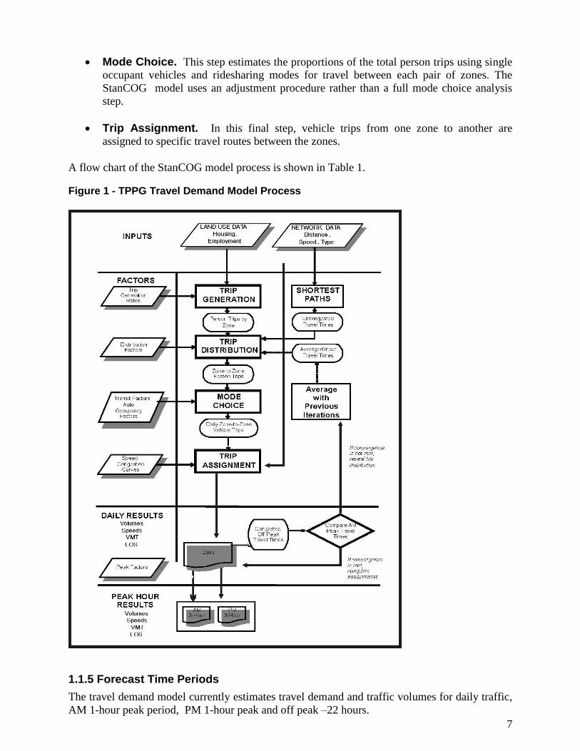
1.1.4 Forecasting Process Four sequential steps (actually sub-models) are involved in the travel demand forecasting
process:
Trip Generation. This initial step translates household and employment data into
person trip ends using trip generation rates established during model calibration.
Trip Distribution. The second general step estimates how many trips travel from one
zone to any other zone. The distribution is based on the number of trip ends generated in
each of the two zones, and on factors that relate the likelihood of travel between any two
zones to the travel time between the two zones.
7
Mode Choice. This step estimates the proportions of the total person trips using single
occupant vehicles and ridesharing modes for travel between each pair of zones. The
StanCOG model uses an adjustment procedure rather than a full mode choice analysis
step.
Trip Assignment. In this final step, vehicle trips from one zone to another are
assigned to specific travel routes between the zones.
A flow chart of the StanCOG model process is shown in Table 1.
Figure 1 - TPPG Travel Demand Model Process
1.1.5 Forecast Time Periods
The travel demand model currently estimates travel demand and traffic volumes for daily traffic,
AM 1-hour peak period, PM 1-hour peak and off peak –22 hours.
8
1.1.6 Feedback Loops
The StanCOG travel model includes a feedback loop that uses the congested speeds estimated
from traffic assignment to recalculate the trip distribution. The feedback loop repeats the process
iteratively until the congested speeds and traffic volumes do not vary significantly between
iterations. This ensures that the congested travel speeds used as input to the air quality analysis
(outside the StanCOG model) are consistent with the travel speeds used throughout the model
process, as required by the Transportation Conformity Rule (40CFR Part 93).
1.1.7 Model Validation
The StanCOG model was revalidated to 2006 daily and peak hour counts . The model estimates
of 2006 daily volumes are within all of the FHWA percent difference targets by facility type. All
model performance measure meet the FHWA criteria. Therefore, the model is considered
acceptable based on FHWA guidelines. The model validation is presented in Appendix A.
1.1.8 Statewide Survey
The StanCOG model uses a variety of inputs based upon the California 2001 statewide
transportation survey. The survey results were combined for Stanislaus County with Merced
County to the south and San Joaquin County to the north in order to increase the sample size (to
roughly 1,500 responses versus only 500 for Stansilaus County by itself). The survey results
form the basis for the friction factors, trip generation rates and peaking factors.
1.2 Transportation Conformity Rule Modeling Requirements
The StanCOG model update and enhancements were designed to provide a network based travel
model that meets the following Transportation Conformity Rule transportation modeling
requirements for serious and above ozone and CO areas with an urbanized population over
200,0001
:
i) Network-based models must be validated against observed counts (peak and off-peak, if
possible) for a base year that is not more than ten years prior to the date of the conformity
determination. Model forecasts must be analyzed for reasonableness and compared to
historical trends and other factors, and the results must be documented.
ii) Land use, population, employment, and other network-based model assumptions must
be documented and based on the best available information.
Transportation Conformity Rule Amendments: Flexibility and Streamlining, Federal Register: August 1990 iii) Scenarios of land development and use must be consistent with the future transportation
system alternatives for which emissions are being estimated. The distribution of
employment and residences for different transportation options must be reasonable.
iv) A capacity-restrained traffic assignment methodology must be used, and emissions
estimates must be based on a methodology which differentiates between peak and off-
peak volumes and speeds, and which uses speeds based on final assigned volumes.
v) Zone-to-zone travel impedances used to distribute trips between origin and destination
pairs must be in reasonable agreement with the travel times that are estimated from final
assigned traffic volumes. Where use of transit currently is anticipated to be a significant
factor in satisfying transportation demand, these times should also be used for modeling

9
mode splits.
vi) Network-based models must be reasonably sensitive to changes in the time(s), cost(s),
and other factors affecting travel choices.
1.3 Procedures to “Run the Model”
Most of the travel demand model procedures have been programmed into the StanCOG job
script. Except for changing the selected year for the network build procedure, this job script
should rarely have to be edited by the user. The user will usually be editing networks (to reflect
the latest information about roadway facilities) and modifying land use assumptions (to reflect
the latest information about development) and then simply applying the model.
The general procedure to apply (or run) the model includes:
1. Document all alternative assumptions
2. Copy master directory
3. Modify “master” network, if necessary
4. Modify the land use / trip generation, if necessary
5. Modify the TP+ job script, if necessary (e.g. change forecast year)
6. “Run” the model alternative
7. Adjust turn or link volumes as necessary
8. View and print the results
These steps are summarized here and discussed in more detail throughout this Model
Documentation Report.
1.3.1 Document all Alternative Changes
All assumptions for the alternative to be run should be adequately documented so that, after
some time has gone by, a user can still identify the land use and network input sources. Network
modifications should be noted on maps or network plots. Land use changes should be printed
out and clearly marked. Ideally, all assumptions would be filed together so that they are easily
accessible in the future.
1.3.2 Copy Master Directory
The generic StanCOG model is stored in a master directory that includes the “Master” network,
the land use / trip generation workbook, the Voyager job script, and all of the supporting files
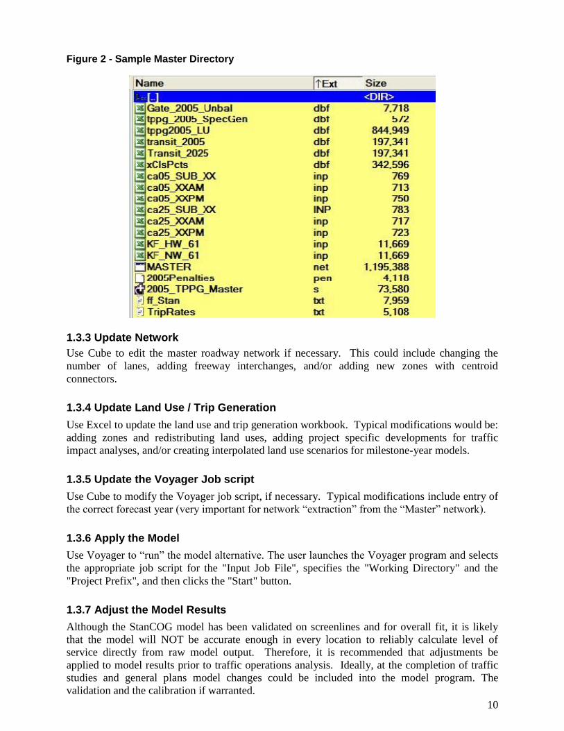
necessary to create a new model alternative. See Figure 2 for a sample master directory. In
order to save the integrity of this data set, the user should make electronic copies of the input
data files by copying the master directory to a new directory (i.e. folder). This can be done using
Windows Explorer or other file management software.
If a model alternative is desired that is based on an already completed model run, simply copy
the input files associated with the previous model alternative to a new directory and follow the
same steps outlined below.
10
Figure 2 - Sample Master Directory
1.3.3 Update Network
Use Cube to edit the master roadway network if necessary. This could include changing the
number of lanes, adding freeway interchanges, and/or adding new zones with centroid
connectors.
1.3.4 Update Land Use / Trip Generation
Use Excel to update the land use and trip generation workbook. Typical modifications would be:
adding zones and redistributing land uses, adding project specific developments for traffic
impact analyses, and/or creating interpolated land use scenarios for milestone-year models.
1.3.5 Update the Voyager Job script
Use Cube to modify the Voyager job script, if necessary. Typical modifications include entry of
the correct forecast year (very important for network “extraction” from the “Master” network).
1.3.6 Apply the Model
Use Voyager to “run” the model alternative. The user launches the Voyager program and selects
the appropriate job script for the "Input Job File", specifies the "Working Directory" and the
"Project Prefix", and then clicks the "Start" button.
1.3.7 Adjust the Model Results
Although the StanCOG model has been validated on screenlines and for overall fit, it is likely
that the model will NOT be accurate enough in every location to reliably calculate level of
service directly from raw model output. Therefore, it is recommended that adjustments be
applied to model results prior to traffic operations analysis. Ideally, at the completion of traffic
studies and general plans model changes could be included into the model program. The
validation and the calibration if warranted.
11
1.3.8 View and Report Model Results
There are a variety of ways to report the results of the CUBE traffic distribution and assignment,
including screen graphics, plots and texts reports.
2. MODEL STUDY AREA AND ZONE SYSTEM
The study area for the TPPG model covers all of Stanislaus County, including the cities of
Modesto, Turlock, Ceres, Oakdale, Riverbank, Patterson, Hughson, Waterford and Newman.
The county is broken up into approximately 2,500 traffic analysis zones (TAZs) with unused
zones set aside for a total of 3,200 possible zones including gateways. Figure 4 shows the travel
demand model TAZs.
The TAZ polygon shapefiles are maintained in ArcView and can be viewed in Viper these are
provided with the default model.
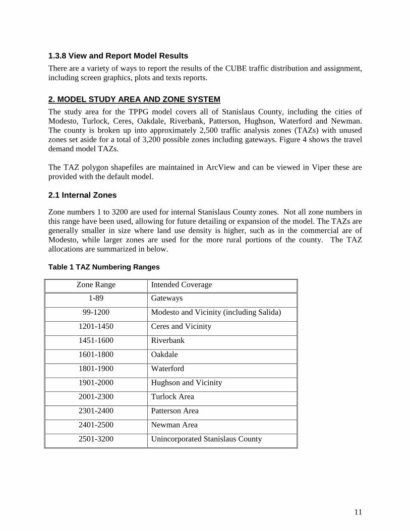
2.1 Internal Zones
Zone numbers 1 to 3200 are used for internal Stanislaus County zones. Not all zone numbers in
this range have been used, allowing for future detailing or expansion of the model. The TAZs are
generally smaller in size where land use density is higher, such as in the commercial are of
Modesto, while larger zones are used for the more rural portions of the county. The TAZ
allocations are summarized in below.
Table 1 TAZ Numbering Ranges
Zone Range Intended Coverage
1-89 Gateways
99-1200 Modesto and Vicinity (including Salida)
1201-1450 Ceres and Vicinity
1451-1600 Riverbank
1601-1800 Oakdale
1801-1900 Waterford
1901-2000 Hughson and Vicinity
2001-2300 Turlock Area
2301-2400 Patterson Area
2401-2500 Newman Area
2501-3200 Unincorporated Stanislaus County
12
2.2 External Zones
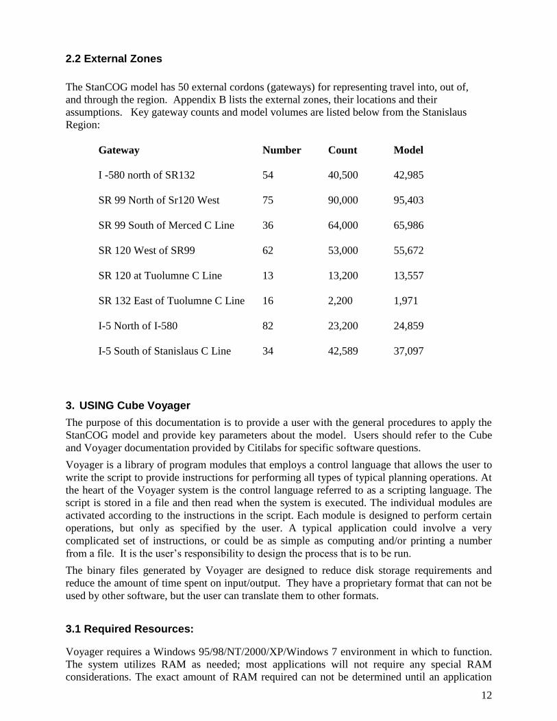
The StanCOG model has 50 external cordons (gateways) for representing travel into, out of,
and through the region. Appendix B lists the external zones, their locations and their
assumptions. Key gateway counts and model volumes are listed below from the Stanislaus
Region:
Gateway Number Count Model
I -580 north of SR132 54 40,500 42,985
SR 99 North of Sr120 West 75 90,000 95,403
SR 99 South of Merced C Line 36 64,000 65,986
SR 120 West of SR99 62 53,000 55,672
SR 120 at Tuolumne C Line 13 13,200 13,557
SR 132 East of Tuolumne C Line 16 2,200 1,971
I-5 North of I-580 82 23,200 24,859
I-5 South of Stanislaus C Line 34 42,589 37,097
3. USING Cube Voyager The purpose of this documentation is to provide a user with the general procedures to apply the
StanCOG model and provide key parameters about the model. Users should refer to the Cube
and Voyager documentation provided by Citilabs for specific software questions.
Voyager is a library of program modules that employs a control language that allows the user to
write the script to provide instructions for performing all types of typical planning operations. At
the heart of the Voyager system is the control language referred to as a scripting language. The
script is stored in a file and then read when the system is executed. The individual modules are
activated according to the instructions in the script. Each module is designed to perform certain
operations, but only as specified by the user. A typical application could involve a very
complicated set of instructions, or could be as simple as computing and/or printing a number
from a file. It is the user‟s responsibility to design the process that is to be run.
The binary files generated by Voyager are designed to reduce disk storage requirements and
reduce the amount of time spent on input/output. They have a proprietary format that can not be
used by other software, but the user can translate them to other formats.
3.1 Required Resources:
Voyager requires a Windows 95/98/NT/2000/XP/Windows 7 environment in which to function.
The system utilizes RAM as needed; most applications will not require any special RAM
considerations. The exact amount of RAM required can not be determined until an application
13
actually runs and the combination of user options is diagnosed. It is fairly safe to state that if a
computer can run Windows, it has enough RAM to run Voyager.
About 2 MB of disk space is required to store the system. Additional disk space is required for
the various files. A typical application will require zonal data files, networks, and matrices.
Zonal data files are not very large, and network sizes will depend upon the number of
alternatives and variables that the user wishes to employ. The largest networks will be only a few
MB. The largest storage requirements will be associated with matrices. A matrix will contain
zones*zones cells of information. Each cell value can be from 0 to 9 bytes in size, but Voyager
uses a proprietary data compression technique that helps to reduce the sizes. The user can control
the matrix sizing.
The minimum recommended hardware (for TP+ without Cube or Viper) is:
Pentium class PC
512 MB of RAM
1 GB hard disk
Generic Printer
Any reasonable monitor
Typical Windows printer drivers are required if Voyager is requested to do plotting
Voyager is designed to run in a multitasking environment. In such an environment, there is a
possibility that several simultaneous applications could try to access the same data files
simultaneously. This could possibly cause problems if one application is trying to update a file
while other applications are accessing it. Different operating systems may handle this conflict
differently. Voyager currently does nothing specifically to deal with this.
3.2 Directories
The Cube and Voyager software are typically installed in the C:\Program Files\Citilabs directory
and subdirectories. These files do not need to be modified or accessed unless the user is
updating the software from the web site or using a CD distributed by Citilabs.
As discussed above, each model alternative should be run and stored in a separate subdirectory.
This includes all associated input and output files.
Geographic files that are common to all alternatives (such as the TIGER street map and the zone
boundaries) may be stored in a single directory rather than copied to each alternative.
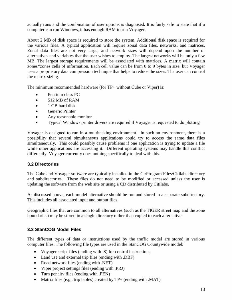
3.3 StanCOG Model Files
The different types of data or instructions used by the traffic model are stored in various
computer files. The following file types are used in the StanCOG Countywide model:
Voyager script files (ending with .S) for control instructions
Land use and external trip files (ending with .DBF)
Road network files (ending with .NET)
Viper project settings files (ending with .PRJ)
Turn penalty files (ending with .PEN)
Matrix files (e.g., trip tables) created by TP+ (ending with .MAT)
14
Report files created by Voyager (ending with .PRN)
Miscellaneous text output files (ending with .VAR, or .TXT)
The following sections describe the input and output files. In this description, "y" characters are
used as placeholders for numbers (“yy”). For example, "20yy_LU.dbf" means any file name that
begins with 20, followed by two other numbers, and ends with "_LU.dbf" (such as,
2025_LU.dbf)
The input files for the full model run are listed in Table 2.
Table 2 - TPPG Model Input Files
File Name Description Created
Using
20yy_Master.s Main TP+ script file for analysis year 20YY Viper
TripRates.txt Cross classified HH and employee trip generation rates MS Excel
MASTER.net Input master road network Viper
20yyPenalties.pen Turn penalties for year 20YY Viper
ff_Stan.txt Friction factors MS Excel
KF_HW_61.inp Home based work K-factors (set to 1.0 by default) MS Excel
KF_NW_61.inp Non work K-factors (set to 1.0 by default) MS Excel
CAyy_SUB_XX.inp Year 20yy Statewide Model Subarea external to external trips MS Excel
CAyy_XXAM.inp Year 20yy AM peak hour external to external trips MS Excel
CAyy_XXPM.inp Year 20yy AM peak hour external to external trips MS Excel
XCLSPcts.dbf cross classification seed file MS Excel
TPPG20yy_LU.dbf Land Use data file MS Excel
TPPG_20yy_SpecGen.dbf Year 20yy special generators file MS Excel
Gate_20yy_Unbal.dbf Unbalanced IX trip generation MS Excel
Note, all files created with MS Excel are editable with a text editor.
3.4 Model Application
Model application (i.e., "running the model") refers to the calculations that convert the data
inputs into results. In Voyager, the program reads a set of instructions in a script file that tell the
computer to use selected Voyager programs and operate on selected data files. The data files
must already be edited and placed in the current subdirectory. In some cases, the script must also
be edited so that it contains the correct instructions and titles.
3.4.1 Script Files
The standard script file, "20yy_Master.s ", has been arranged to make it easy to run a new
alternative. The first part of the script lists the important input files. Use this as a checklist for
preparing files. The analysis year can be changed by modifying one line of code.
Lines beginning with a semicolon (;) are comments that are ignored by the program and are
added for clarity or documentation. The user can also add additional comment lines beginning
with a semicolon (;).
3.4.2 Scenario Name
Each model alternative should have a unique scenario name (also known as "project prefix").
Similar to MINUTP (the software the MOGP model used previously), the scenario name is used
15
to identify important input and output files. It is also recommended that the subdirectory name
incorporate the scenario name. The Voyager software restricts the user to four characters. The
default name is TPPG.
3.4.3 Running Voyager
Once all the input files have been updated and included in the model alternative directory, the
user is ready to start Voyager.
If Voyager has been properly installed, there should be a Voyager icon on the desktop that can be
used to launch Voyager. Click on the Voyager icon and the Voyager control screen will appear.
If there is no icon, Voyager can be started from the Start Menu like any other program in
Windows. Voyager can also be started directly from within Cube. From the Cube menu, choose
Run and then either File, Current File, Select Text, or Current Step, whichever is appropriate. If
starting Voyager from Cube, be sure that any of the files that are to be used during the Voyager
application are not left open in Cube while the Voyager application is executing.
Once Voyager has been activated, the Voyager window will open and prompt the user for
the following items:
The name of the script file that is to be run (if not shown the user can select the "Browse"
button to select the correct script file in the correct subdirectory);
The working directory where the basic application data is stored (this should default to
the directory where the job script file resides when a new job script file is selected);
A system prefix (make certain that the Project Prefix matches the scenario you have
selected, such as "TPPG", and is a max of 4 characters - ALWAYS VERIFY THIS.);
The desired height and width of a printed page (usually the default isn‟t modified); and
An ID that will be printed at the top of every printed page (descriptive text for your
alternative).
Press "Start"
When this data is completed, the Start Button is pressed, and Voyager begins execution. As it is
executing, periodic messages will be written to the message box. The program window can be
minimized or left open as Voyager is executing. The X button allows for pre-mature termination
of the application. When the application is finished, the View Print File button can be pushed to
view the printed results.
3.4.4 Errors
If there is an error, the Voyager control screen will display a message such as "Return Code 2."
The only description of the error is contained in the .PRN file created by Voyager.
Select "View Print File." Press the <F3> function key to move to the first error message.
4. MODIFYING THE ROADWAY NETWORK
The StanCOG regional travel model uses coded representations of the region‟s existing and
future roadway networks that can be edited for alternative year scenarios.

16
4.1 Road Network Elements
The road network is a computerized representation of the major street and highway system
within the study area. The more important streets (freeways, expressways, arterials, and
collectors) are fully included in the network. The model does not explicitly include all local
streets. Some minor collector streets, local streets and driveways are instead represented by
simplified network links (“zone centroid connectors”) that represent local connections to the
adjacent major roadway network. The coded road network is comprised of three basic types of
data: nodes, links and turn penalties.
4.1.1 Nodes
Nodes are established at each and every intersection between two or more links. Nodes are
assigned numbers, with the first 3200 node numbers in the TPPG model representing traffic
analysis zones (TAZ) as discussed above.
The road network nodes are coded with geographical “X” and “Y” coordinates to permit plotting
and graphic displays. As part of the PROJECT, the roadway network was projected to State
Plane 1983, California Zone 4 coordinates, with measurement in feet. Additionally, individual
nodes were moved geographically to allow the model network to overlay in a consistent manner
with other geographical information such as census maps.
Node data includes the node number, the X and Y coordinates, a City code filed, and separate
numbering for TAZ and Gateway nodes (the same number as the node number).
4.1.2 Links
Links represent road segments, and are uniquely identified by the node numbers at each end of
the segment (for example, a link may be identified as “1232-1234”). Information is coded for
each road link.
4.2 “Master” Roadway Network
StanCOG staff developed a “Master” network to store the network related attributes for the 2006
base network including number of lanes, facility type. Capacity-increasing roadway network
improvements are in the Master network with construction year (project completion=year and
proj_ID) identifiers. All roadway networks used in the travel demand model are “built” from
this Master network. The purpose of creating a Master network was to make the task of network
maintenance more efficient. In the past, if a roadway network improvement was to be included
in several alternatives, the same network editing had to be performed individually for each of the
network years. With a Master network, the user need only input the improvement in one place
with the appropriate year of construction and then all desired network years can be built and will
be consistent.
While the creation of a Master network will make the task of network maintenance more
efficient, it will require the user to be aware of how network coding is handled and to be diligent
about displaying proper network data. Figure 4 shows an example of the Master network coding
that illustrates the need for user diligence.
This figure shows a base year location with at-grade intersections that will become a grade-
separated interchange in the future. The base year and future links are shown in different widths
and two of the nodes (3990 and 3992 in this hypothetical example) are shown exaggeratedly
offset for clarity. The dashed links are included in both the base year network and in the future

17
network. The light weight solid links are included in the base year network but are excluded
from the future network. The heavy weight links are included in the future network but are
excluded from the base year network.
The display of these links in the master network can be confusing, because there are duplicate
links for connecting the extremes of the interchange facility and the nodes are not normally
offset as shown in Figure 4. One set of links is for the base year and one set is for the future
year. When creating or editing such links care must be taken to add or change nodes and links so
that the desired future network will be produced. The section titled Building the Future Year
Roadway Network, below, describes how the link attributes are used to create the future network.
Figure 4 - Example of Master Network Coding
Base Year Links 2205-3990* 3990-3992* 3992-2408* 2559-3990 3990-2560 3705-3992 3992-3706 Future Year Links 2205-2408* 2559-2560 3705-3706 2559-2205 2205-2560 3705-2408 2408-3706 * = two-way link
4.2.1 Editing the Master Roadway Network
If new or revised roadway facility projects are identified in the future that are not already
included in the Master network, changes will need to be made to the Master network. Such
changes might include adding links that are not already in the Master network, changing the
number of lanes for links that are already present or deleting links that are already present.
To add a link: First copy a link that is similar to the one you want to add. Next,
click and hold the left mouse button down when the cursor is on the A-
node location then drag the mouse cursor to the B-node location and
release the mouse button. If the selected location is within the search
tolerance to an existing node, the end point of the new link will snap to
this node; otherwise, the program prompts the user to add a new node
and requests the new node number. A list of unused nodes will be
displayed in the new node dialog box and the new number can then be
selected from the list of unused nodes or entered manually. Then, enter
or change the various link attributes to properly represent the link you

18
are adding.
To widen a link: Click on the link to select it. The attributes for the link will be
displayed in a dialog box. Change the LANES_IMP and IMP_MOGP
attributes to properly represent the widening. If it is a two-way link,
change the attributes for both travel directions (A-to-B and B-to-A).
To delete a link: Click on the link to select it, then press the Delete key.
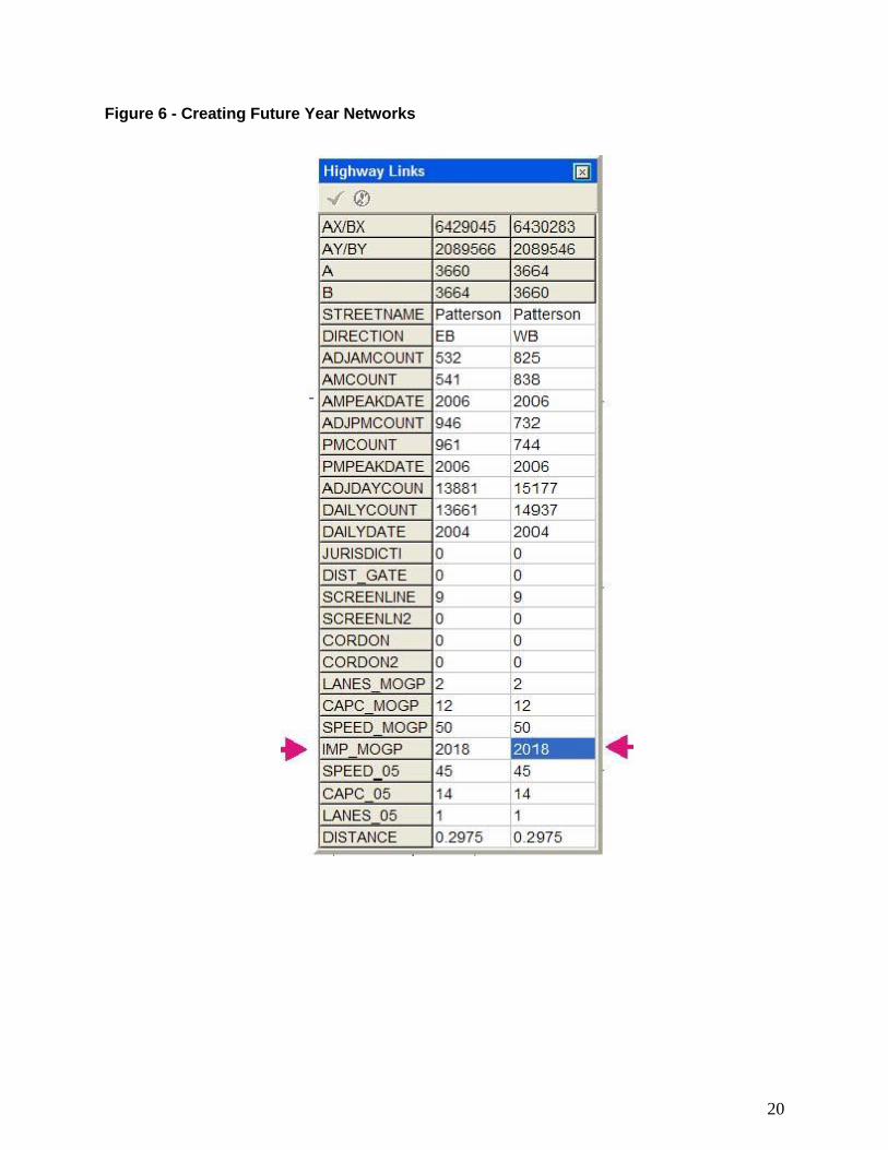
4.2.2 Building the Future Year Roadway Network As discussed above, links for all base year and future year improvements are included in the
Master network. Future year roadway networks are created by including future links or changing
the number of lanes and the speed and capacity classes on appropriate links. In some cases, it
will be necessary to exclude base year links (e.g., if an at-grade intersection is being improved to
a grade-separated crossing, the links that are attached to the node where the current at-grade
condition exists must be excluded).
This process of including, changing, and/or excluding links is accomplished dynamically as the
model is run. The information stored in each link's attributes is used to determine whether the
link will be included, or changed, or excluded. The attributes that control this process are
IMP_YEAR (the year when the improvement is to become effective), LANES06 (the base year
number of lanes for the link), and LANES_MOGP (the improved number of lanes for the link).
IT IS IMPERATIVE THAT FOR EACH RUN THE ANALYSIS YEAR IN THE SCRIPT BE
PROPERLY SET.
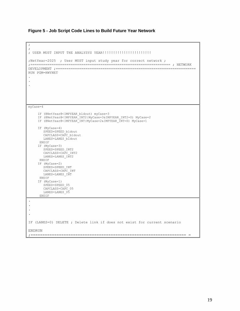
The portion of script shown in Figure 5 uses these attributes to extract or build the correct
roadway network for the defined alternative year. Figure 5 shows how these attributes are used to
accomplish the three basic improvement actions (include, change, and exclude). If the analysis
year in the script is later than the IMP_Year for the model scenario, the number of lanes, speed
and capacity class for the model scenario will be included in the run. All future network and
specific network improvements can be tracked by highlighting the variable Proj_ID and
LanesXX (Year).
19
Figure 5 - Job Script Code Lines to Build Future Year Network
;
;
; USER MUST INPUT THE ANALYSYS YEAR!!!!!!!!!!!!!!!!!!!!!!!
;NetYear=2025 ; User MUST input study year for correct network ;
;================================================================== ; NETWORK
DEVELOPMENT ;==================================================================
RUN PGM=HWYNET
.
.
.
myCase=4
IF (@NetYear@<IMPYEAR_bldout) myCase=3
IF (@NetYear@<IMPYEAR_INT2|MyCase=3&IMPYEAR_INT2=0) MyCase=2
IF (@NetYear@<IMPYEAR_INT|MyCase=2&IMPYEAR_INT=0) MyCase=1
IF (MyCase=4)
SPEED=SPEED_bldout
CAPCLASS=CAPC_bldout
LANES=LANES_bldout
ENDIF
IF (MyCase=3)
SPEED=SPEED_INT2
CAPCLASS=CAPC_INT2
LANES=LANES_INT2
ENDIF
IF (MyCase=2)
SPEED=SPEED_INT
CAPCLASS=CAPC_INT
LANES=LANES_INT
ENDIF
IF (MyCase=1)
SPEED=SPEED_05
CAPCLASS=CAPC_05
LANES=LANES_05
ENDIF
.
.
.
.
IF (LANES=0) DELETE ; Delete link if does not exist for current scenario
ENDRUN
;================================================================== =
20
Figure 6 - Creating Future Year Networks
21
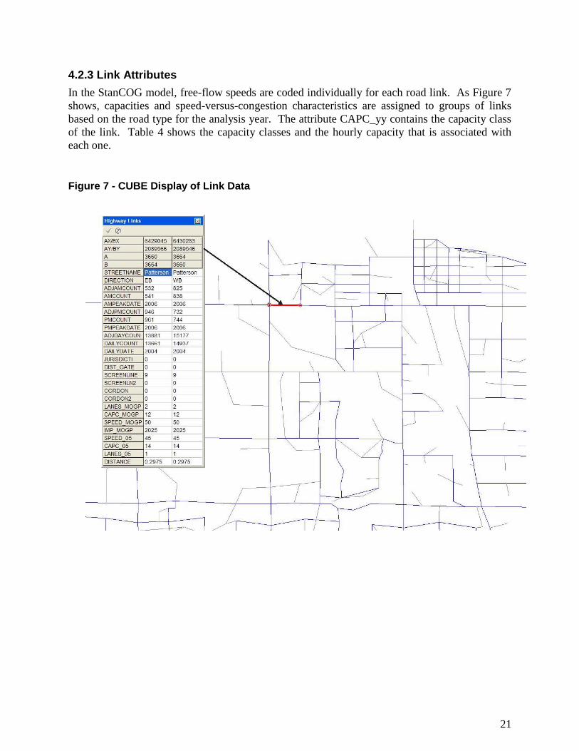
4.2.3 Link Attributes
In the StanCOG model, free-flow speeds are coded individually for each road link. As Figure 7
shows, capacities and speed-versus-congestion characteristics are assigned to groups of links
based on the road type for the analysis year. The attribute CAPC_yy contains the capacity class
of the link. Table 4 shows the capacity classes and the hourly capacity that is associated with
each one.
Figure 7 - CUBE Display of Link Data
22
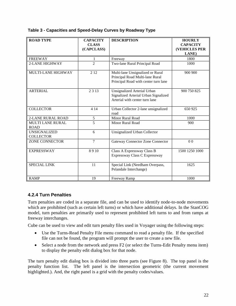
Table 3 - Capacities and Speed-Delay Curves by Roadway Type
ROAD TYPE CAPACITY
CLASS
(CAPCLASS)
DESCRIPTION HOURLY
CAPACITY
(VEHICLES PER
LANE)
FREEWAY 1 Freeway 1800
2-LANE HIGHWAY 2 Two-lane Rural Principal Road 1000
MULTI-LANE HIGHWAY 2 12 Multi-lane Unsignalized or Rural
Principal Road Multi-lane Rural
Principal Road with center turn lane
900 900
ARTERIAL 2 3 13 Unsignalized Arterial Urban
Signalized Arterial Urban Signalized
Arterial with center turn lane
900 750 825
COLLECTOR 4 14 Urban Collector 2-lane unsignalized
road
650 925
2-LANE RURAL ROAD 5 Minor Rural Road 1000
MULTI LANE RURAL
ROAD
5 Minor Rural Road 900
UNSIGNALIZED
COLLECTOR
6 Unsignalized Urban Collector
ZONE CONNECTOR 7 Gateway Connector Zone Connector 0 0
EXPRESSWAY 8 9 10 Class A Expressway Class B
Expressway Class C Expressway
1500 1250 1000
SPECIAL LINK 11 Special Link (Needham Overpass,
Pelandale Interchange)
1625
RAMP 19 Freeway Ramp 1000
4.2.4 Turn Penalties
Turn penalties are coded in a separate file, and can be used to identify node-to-node movements
which are prohibited (such as certain left turns) or which have additional delays. In the StanCOG
model, turn penalties are primarily used to represent prohibited left turns to and from ramps at
freeway interchanges.
Cube can be used to view and edit turn penalty files used in Voyager using the following steps:
Use the Turns-Read Penalty File menu command to read a penalty file. If the specified
file can not be found, the program will prompt the user to create a new file.
Select a node from the network and press F2 (or select the Turns-Edit Penalty menu item)
to display the penalty edit dialog box for that node.
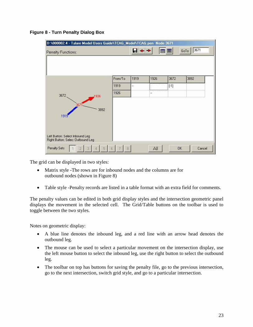
The turn penalty edit dialog box is divided into three parts (see Figure 8). The top panel is the
penalty function list. The left panel is the intersection geometric (the current movement
highlighted.). And, the right panel is a grid with the penalty codes/values.
23
Figure 8 - Turn Penalty Dialog Box
The grid can be displayed in two styles:
Matrix style -The rows are for inbound nodes and the columns are for
outbound nodes (shown in Figure 8)
Table style -Penalty records are listed in a table format with an extra field for comments.
The penalty values can be edited in both grid display styles and the intersection geometric panel
displays the movement in the selected cell. The Grid/Table buttons on the toolbar is used to
toggle between the two styles.
Notes on geometric display:
A blue line denotes the inbound leg, and a red line with an arrow head denotes the
outbound leg.
The mouse can be used to select a particular movement on the intersection display, use
the left mouse button to select the inbound leg, use the right button to select the outbound
leg.
The toolbar on top has buttons for saving the penalty file, go to the previous intersection,
go to the next intersection, switch grid style, and go to a particular intersection.
24
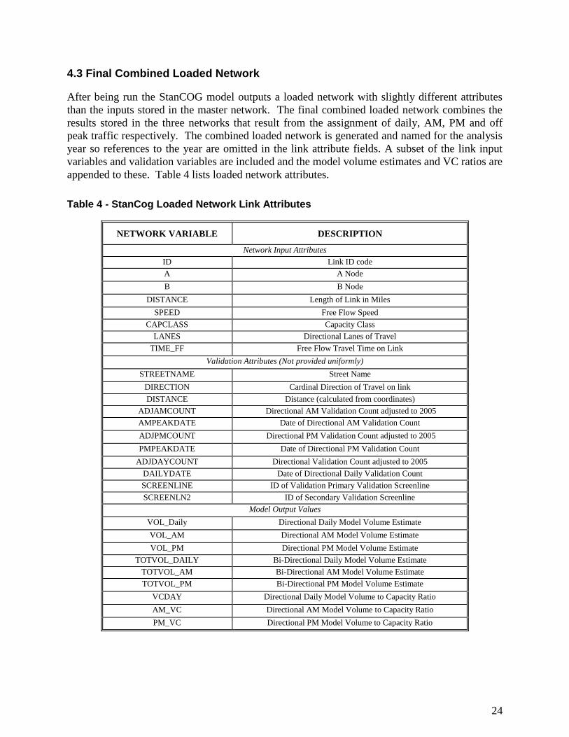
4.3 Final Combined Loaded Network
After being run the StanCOG model outputs a loaded network with slightly different attributes
than the inputs stored in the master network. The final combined loaded network combines the
results stored in the three networks that result from the assignment of daily, AM, PM and off
peak traffic respectively. The combined loaded network is generated and named for the analysis
year so references to the year are omitted in the link attribute fields. A subset of the link input
variables and validation variables are included and the model volume estimates and VC ratios are
appended to these. Table 4 lists loaded network attributes.
Table 4 - StanCog Loaded Network Link Attributes
NETWORK VARIABLE DESCRIPTION
Network Input Attributes
ID Link ID code
A A Node
B B Node
DISTANCE Length of Link in Miles
SPEED Free Flow Speed
CAPCLASS Capacity Class
LANES Directional Lanes of Travel
TIME_FF Free Flow Travel Time on Link
Validation Attributes (Not provided uniformly)
STREETNAME Street Name
DIRECTION Cardinal Direction of Travel on link
DISTANCE Distance (calculated from coordinates)
ADJAMCOUNT Directional AM Validation Count adjusted to 2005
AMPEAKDATE Date of Directional AM Validation Count
ADJPMCOUNT Directional PM Validation Count adjusted to 2005
PMPEAKDATE Date of Directional PM Validation Count
ADJDAYCOUNT Directional Validation Count adjusted to 2005
DAILYDATE Date of Directional Daily Validation Count
SCREENLINE ID of Validation Primary Validation Screenline
SCREENLN2 ID of Secondary Validation Screenline
Model Output Values
VOL_Daily Directional Daily Model Volume Estimate
VOL_AM Directional AM Model Volume Estimate
VOL_PM Directional PM Model Volume Estimate
TOTVOL_DAILY Bi-Directional Daily Model Volume Estimate
TOTVOL_AM Bi-Directional AM Model Volume Estimate
TOTVOL_PM Bi-Directional PM Model Volume Estimate
VCDAY Directional Daily Model Volume to Capacity Ratio
AM_VC Directional AM Model Volume to Capacity Ratio
PM_VC Directional PM Model Volume to Capacity Ratio
25
4.4 Transit Network
The StanCOG travel model does not include a separate transit network. Based on the Caltrans
2000 Travel Survey, transit trips (not including school buses) account for a negligible portion of
trips in Stanislaus County. This proportion is not expected to increase significantly in the future
with the current Regional Transportation Plan.
Future regional transportation studies may require more detailed analysis of transit infrastructure
investments. If so, the StanCOG travel model capabilities could be enhanced by adding separate
representation of the transit systems and a mode choice analysis step. The peak period model
structure is compatible with transit and mode choice procedures used for other California travel
models such as Fresno County. StanCog is prepared to include transit assignments and mode
choice in 2010-2011 fiscal year.
5. LAND USE / EXTERNAL TRIP ASSUMPTIONS
Land use and socioeconomic data at the traffic analysis zone level are used for determining trip
generation. The StanCOG model maintains the previous zonal variables for the land
use/socioeconomic database, including housing units by single-family and multiple-family use
and auto occupancy, and employment by category (retail, service, education, government, and
other). A TAZ map of the zonal structure is provided in GIS and *.pdf format with the default
files.
Land use and socio-economic data, as well as information on special generators and external
trips are all accessible and editable in Microsoft Excel. When so accessed the formats are
intended to allow the user to easily modify land use assumptions and re-export these files out as
.DBF files the required files needed to run the StanCOG model.
5.1 Household Cross Classification Data
Auto ownership data and Household size data were obtained from the 2000 Census and a
household cross classification scheme developed for household trip generation. The percentages
of 0, 1, 2, 3, and for or more auto household were indexed against households of size 1, 2, 3, 4, 5
or more for both single family and multifamily dwellings. For each TAZ containing housing an
estimate is therefore available for the proportion of households falling within any one of fifty
categories each having its own set of trip generation rates. This data is contained in the file
xClsPct.dbf. For housing in new zones this file is used to estimate cross classification
proportions by applying a regression equation against other land use variables. The user has the
option of editing the xClsPct.dbf file directly to input the proportions of households with
different levels of auto ownership and different numbers of persons. The totals for auto
ownership and household size must add up to 1 in both cases this is not recommended for any
but the most advanced users.
The 2006 employment data in the updated model is primarily based on the land use database
from the previous version of the model. The land use database in the previous version of the
StanCOG model was based on an extensive compilation of acreages by community plan land use
category in each community. Occupied acreages were converted to building area and numbers
of employees using standard density factors.
26
The most recent available information on the numbers of Stanislaus County employees in each
employment category were obtained from the 2005 California State Profile (Woods and Poole
Economics, Inc. 2006 and the Employment Development Department EDD 2006). Factors were
applied so that the countywide totals of each employee type would match 2006 employment
totals reported by EDD.
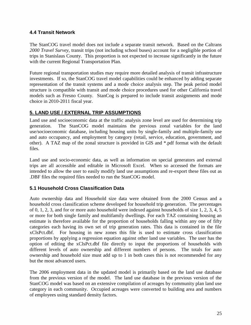
Table 5 shows the cross-classified household data for 2006 Table 25 shows the same data for
2030.
Table 5 2006 Countywide Cross Classified Summary
Land Use assumptions for the rest of the county were based on the 2006 update of the StanCOG
model which incorporates countywide land use projections apportioned among the various
jurisdictions by StanCOG staff.
Table 6 2030 Future Year Land Use Summaries

27
5.2 Modifying Land Use Assumptions
The land use data used by default in the model are contained in the TPPG2006_LU.dbf and
TPPG2030_LU.dbf files these are the base year land use and the 2030 horizon year land use
inputs).
The base year land use data represents the latest land use inventory as of the date of this model
update, and hence represents the year 2006 land use status. These data are consistent with the
validation run, and the user is expected to maintain this consistency unless errors are found and
need to be corrected.
Future horizon year (2030) land uses can be redistributed based on new input from local
jurisdictions, or to reflect new project specific land use proposals. If alternative scenarios to the
adopted buildout land use scenario are being tested, the adopted file should be backed up and
maintained in a separate directory.
To make changes in the 2030 land use input data, modify the information for the appropriate
TAZ in the 2030 land use find the TAZ in the left most column and make the appropriate
changes in housing and/or employment levels to represent the total levels with the land use
changes that are being made. The fields in the land use file are
TAZ = Traffic Analysis Zone Number Juris= jurisdiction/CDP AREA = Land Area in Acres POP = Population SF = Single Family households MF = Multi Family households RET = Retail Employees SER = Service Employees EDU = Educational Employees GOV = Government Employees OTH = Other Category Employees Note that the POP column must be updated as the various household variables are changed. The
default for population is 2.9 persons per SF or MF household. If the user desires to split a TAZ,
then changes will have to be made to add one or more new TAZs to both the base year and the
horizon year land use files. Appropriate data for the old TAZ and the new TAZ(s) will need to
be entered on each worksheet.
28
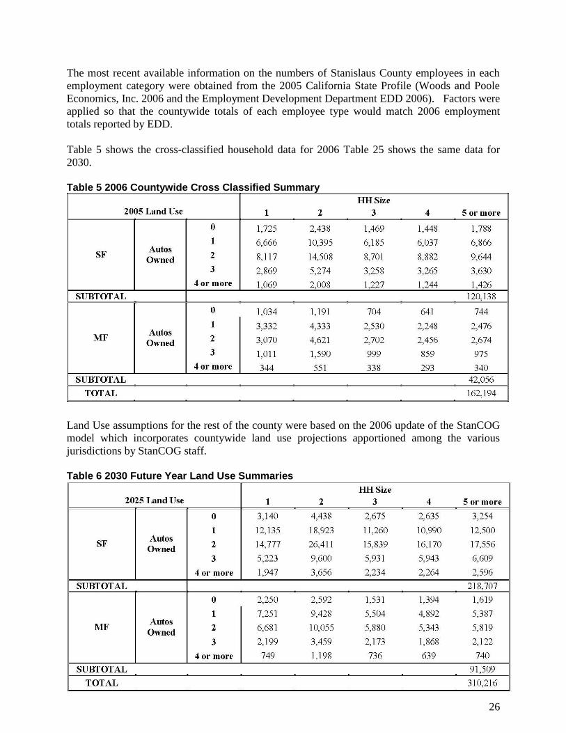
Figure 9 - Portion of the 2030 Land Use Database
5.3 Using Special Generators
The model is capable of incorporating “special generators” within Stanislaus County. These are
included in the Spec Gen worksheet (trip generation for special generators). Special generators
are used to include trips from land uses that are not well represented by the standard land use
categories or trip rates. In the StanCOG model, special generation is input directly as person trips
by trip purpose this may require the analyst to estimate the distribution of trips by purpose and
will require the analyst to apply vehicle occupancy factors to convert person trips to vehicle trips.
Often the estimation of trips by purpose is obviated by the fact that special generators are input
as Home Based Other trips to reflect categories that are not reflected by other purposes (such as
recreational attractions). The distribution can also be estimated based on similar zones (by
reference to the output file “TPPG_input_PA.dbf” generated by the model). Or can be calculated
for trip attractors by multiplying the employment times the trip generation rates (see appendix).
Once the distribution by trip purpose is determined vehicle trips are converted into person trips
by using the vehicle occupancy factors embedded into the model and shown in the appendix.
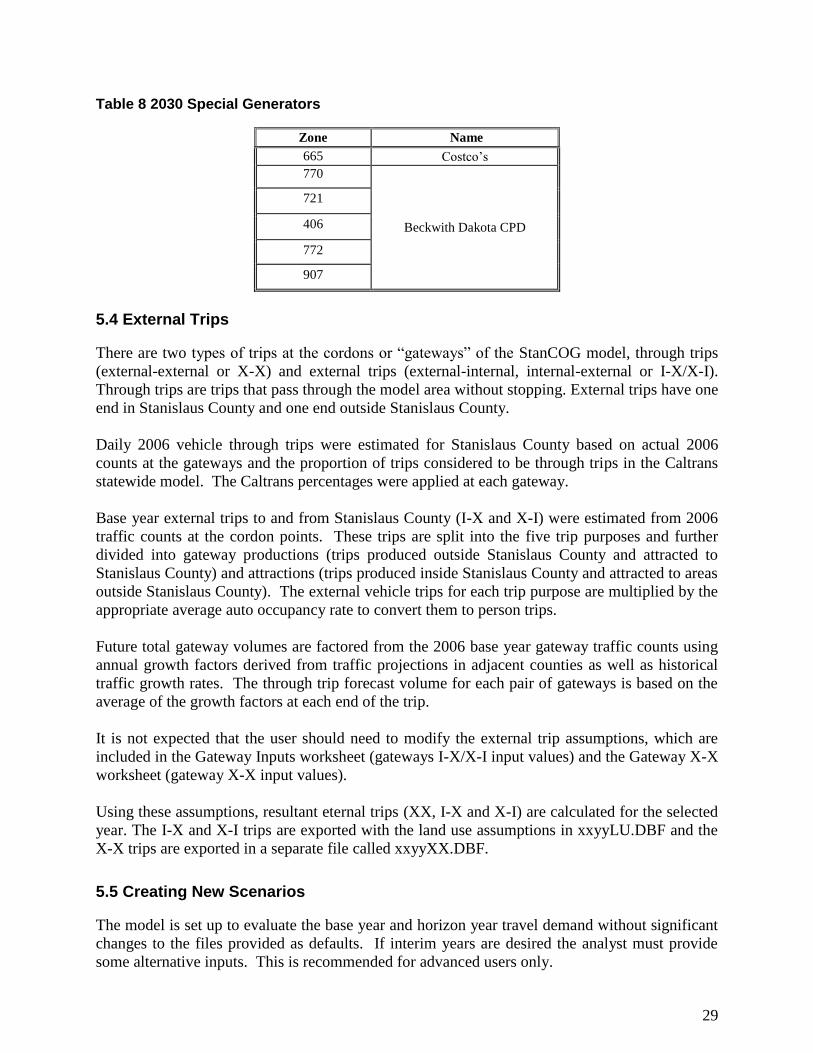
New special generators should be appended to the file TPPG_20XX_SPECGEN.dbf. shows the
special generator zones for the 2025 scenario.
29
Table 8 2030 Special Generators
Zone Name
665 Costco‟s
770
Beckwith Dakota CPD
721
406
772
907
5.4 External Trips
There are two types of trips at the cordons or “gateways” of the StanCOG model, through trips
(external-external or X-X) and external trips (external-internal, internal-external or I-X/X-I).
Through trips are trips that pass through the model area without stopping. External trips have one
end in Stanislaus County and one end outside Stanislaus County.
Daily 2006 vehicle through trips were estimated for Stanislaus County based on actual 2006
counts at the gateways and the proportion of trips considered to be through trips in the Caltrans
statewide model. The Caltrans percentages were applied at each gateway.
Base year external trips to and from Stanislaus County (I-X and X-I) were estimated from 2006
traffic counts at the cordon points. These trips are split into the five trip purposes and further
divided into gateway productions (trips produced outside Stanislaus County and attracted to
Stanislaus County) and attractions (trips produced inside Stanislaus County and attracted to areas
outside Stanislaus County). The external vehicle trips for each trip purpose are multiplied by the
appropriate average auto occupancy rate to convert them to person trips.
Future total gateway volumes are factored from the 2006 base year gateway traffic counts using
annual growth factors derived from traffic projections in adjacent counties as well as historical
traffic growth rates. The through trip forecast volume for each pair of gateways is based on the
average of the growth factors at each end of the trip.
It is not expected that the user should need to modify the external trip assumptions, which are
included in the Gateway Inputs worksheet (gateways I-X/X-I input values) and the Gateway X-X
worksheet (gateway X-X input values).
Using these assumptions, resultant eternal trips (XX, I-X and X-I) are calculated for the selected
year. The I-X and X-I trips are exported with the land use assumptions in xxyyLU.DBF and the
X-X trips are exported in a separate file called xxyyXX.DBF.
5.5 Creating New Scenarios
The model is set up to evaluate the base year and horizon year travel demand without significant
changes to the files provided as defaults. If interim years are desired the analyst must provide
some alternative inputs. This is recommended for advanced users only.
30
1) Set Analysis Year. One line of code in the model script must be modified. The analysis year
entered at the top of the set up portion of the script as the variable ‘NetYear,’ must be set to the
desired year.
2) Provide Interim/Outyear Land Use File. This can based on wholesale inclusion of the
General Plan build out assumptions for various areas of the model where development is
expected to occur (for example for a specific plan or community plan area that is expected to
develop in the interim). This requires specific planning guidance and should involve direction
from the appropriate jurisdictions. An alternative approach is to perform an interpolation
between the 2006 and the 2025 land use files provided for the default model. This is best
accomplished in a spreadsheet where the POP,SF,MF,RET,SER,EDU,GOV, and OTH variables
are calculated for the interim analysis year based on the formula:
Value_[Analysis Year]= Value_2005 + [(Value_2025-Value_2005)*(AnalysisYear-2005)/20]
The resulting worksheet must be saved with the name in the format:
TPPG[Analysis Year]_LU.dbf.
Where [Analysis Year] is substituted with the desired analysis year. This file must be in
*.dbf format. „TPPG‟ is the default prefix and may change accordingly. The special
generators must be edited in Excel and the file renamed .
TPPG_[Analysis Year]_SPECGEN.dbf.
3) Provide Turn Penalty File. Turn penalty files are only provided for the default base
year and general plan year scenarios. The user has the option of selecting the general plan
year file and renaming it according to the convention:
[Analysis Year]penalties.pen
4) Verify Network Improvements. The user must review the Master Network and adjust
improvement years for facilities that will be improved by the by the interim analysis year.
The default improvement year is 2025. The analysis must coordinate with the lead
agency to make these modifications. ALSO it may be necessary to add additional
attributes to the Master network to reflect instances where links are improved but not to
the full general plan level. This is done in viper under the menu item
LINK=>Attribute=>Add. Three attributes should be added and named:
[Analysis Year]Speed
[Analysis Year]Lanes
[Analysis Year]CAPC
The analyst should typically set the values of these attributes to using the menu
commands LINK=>Compute, then modify the links with interim year differences
manually.
31
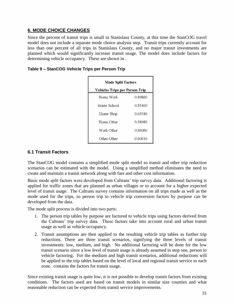
6. MODE CHOICE CHANGES
Since the percent of transit trips is small in Stanislaus County, at this time the StanCOG travel
model does not include a separate mode choice analysis step. Transit trips currently account for
less than one percent of all trips in Stanislaus County, and no major transit investments are
planned which would significantly increase transit usage. The model does include factors for
determining vehicle occupancy. These are shown in .
Table 9 – StanCOG Vehicle Trips per Person Trip
6.1 Transit Factors The StanCOG model contains a simplified mode split model so transit and other trip reduction
scenarios can be estimated with the model. Using a simplified method eliminates the need to
create and maintain a transit network along with fare and other cost information.
Basic mode split factors were developed from Caltrans‟ trip survey data. Additional factoring is
applied for traffic zones that are planned as urban villages or to account for a higher expected
level of transit usage. The Caltrans survey contains information on all trips made as well as the
mode used for the trips, so person trip to vehicle trip conversion factors by purpose can be
developed from the data.
The mode split process is divided into two parts:
1. The person trip tables by purpose are factored to vehicle trips using factors derived from
the Caltrans‟ trip survey data. These factors take into account rural and urban transit
usage as well as vehicle occupancy.
2. Transit assumptions are then applied to the resulting vehicle trip tables as further trip
reductions. There are three transit scenarios, signifying the three levels of transit
investments: low, medium, and high. No additional factoring will be done for the low
transit scenario since a low level of transit usage is already assumed in step one, person to
vehicle factoring. For the medium and high transit scenarios, additional reductions will
be applied to the trip tables based on the level of local and regional transit service to each
zone. contains the factors for transit usage.
Since existing transit usage is quite low, it is not possible to develop transit factors from existing
conditions. The factors used are based on transit models in similar size counties and what
reasonable reduction can be expected from transit service improvements.
32
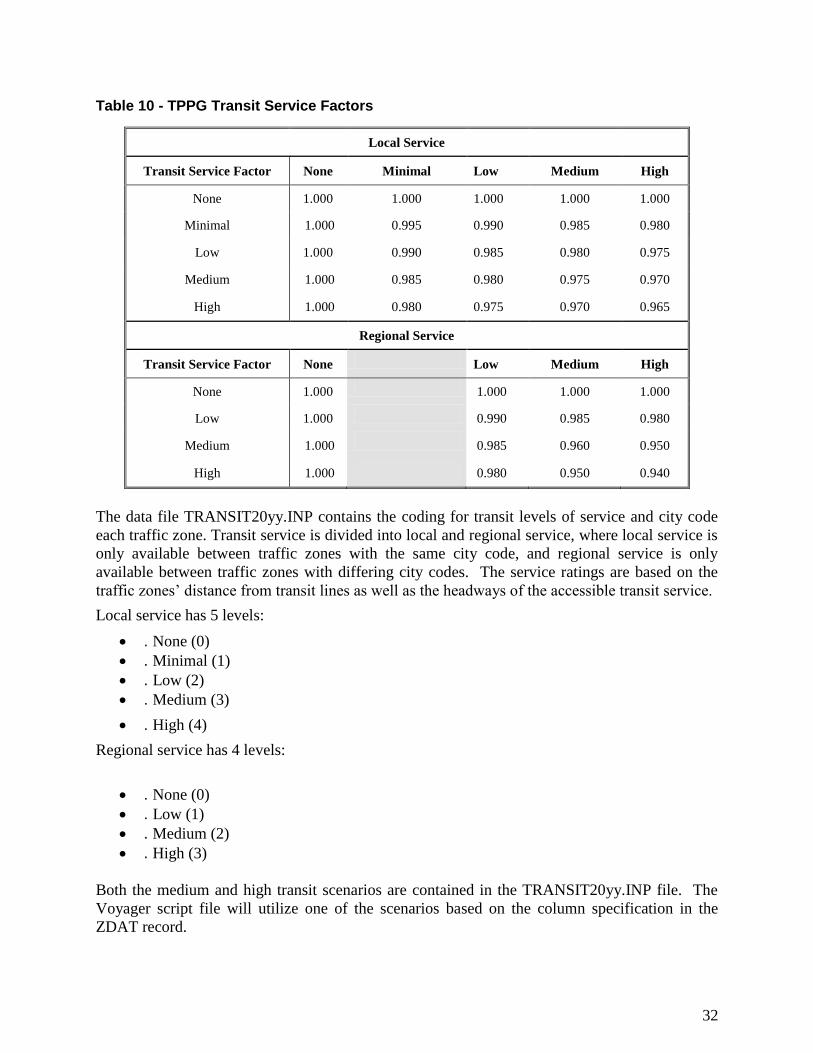
Table 10 - TPPG Transit Service Factors
Local Service
Transit Service Factor None Minimal Low Medium High
None 1.000 1.000 1.000 1.000 1.000
Minimal 1.000 0.995 0.990 0.985 0.980
Low 1.000 0.990 0.985 0.980 0.975
Medium 1.000 0.985 0.980 0.975 0.970
High 1.000 0.980 0.975 0.970 0.965
Regional Service
Transit Service Factor None Low Medium High
None 1.000 1.000 1.000 1.000
Low 1.000 0.990 0.985 0.980
Medium 1.000 0.985 0.960 0.950
High 1.000
0.980 0.950 0.940
The data file TRANSIT20yy.INP contains the coding for transit levels of service and city code
each traffic zone. Transit service is divided into local and regional service, where local service is
only available between traffic zones with the same city code, and regional service is only
available between traffic zones with differing city codes. The service ratings are based on the
traffic zones‟ distance from transit lines as well as the headways of the accessible transit service.
Local service has 5 levels:
. None (0)
. Minimal (1)
. Low (2)
. Medium (3)
. High (4)
Regional service has 4 levels:
. None (0)
. Low (1)
. Medium (2)
. High (3)
Both the medium and high transit scenarios are contained in the TRANSIT20yy.INP file. The
Voyager script file will utilize one of the scenarios based on the column specification in the
ZDAT record.

33
7. SPECIAL ASSIGNMENTS
In an effort to meet the needs of StanCOG and its jurisdictions, several special assignment
options are explained here, including the saving of selected intersection turn volumes, select link
and select zone assignments.
7.1 Intersection Turn Volumes
The Voyager command TURNS is used to request that the volumes at specific nodes are to be
accumulated. If there is at least one TURNS statement, the module will accumulate turns for
every assignment loading. At the end of each iteration (in the Phase=Adjust), a single total turn
volume will be computed for each movement at the nodes where turns are requested. By default,
the single volume is computed by adding all the individual turn volume sets together (T =
TURN[1] + TURN [2] + TURN [..] ...).
If turn volumes are to be accumulated and reported, it is necessary to specify the selected nodes
with an N= , , , etc statement, and also to have a FILEO TURNVOLO specified to define the
file(s) to which the turn volumes will be written. N |IP| is a list of nodes at which turning
volumes are to be accumulated.
A sample job script to save turn volumes is shown in. This job script loads the morning 3-hour
peak period traffic onto the network saving turns at the nodes specified by:
TurnList=1521-1523,1525.
A binary file (.BIN) and a database file (.DBF) are created with the turning volume
output by:
TURNVOLO=TPPG_[Analysis year]AM.TRN,FORMAT=BIN
TURNVOLO=TPPG_[Analysis ear]AM.DBF,FORMAT=DBF
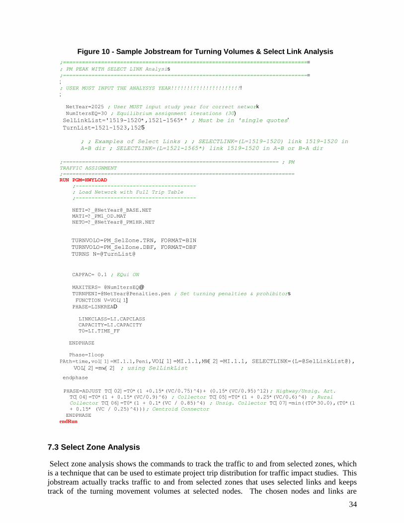
7.2 Select Link Analysis
Select link analysis also shows the commands to track the traffic using a selected link or set of
links. The chosen links are specified by:
SelLinkList='1519-1520*,1521-1565*'
The volumes using the selected links are saved in the output file as a separate link
attribute that is created by:
PATH=TIME,PENI=1,VOL[1]=MI.1.1,MW[2]=MI.1.1,SELECTLINK=
(L=@SelLinkList@), VOL[2]=mw[2]
34
Figure 10 - Sample Jobstream for Turning Volumes & Select Link Analysis
;==============================================================================
; PM PEAK WITH SELECT LINK Analysis
;==============================================================================
; ; USER MUST INPUT THE ANALYSYS YEAR!!!!!!!!!!!!!!!!!!!!!!!
; NetYear=2025 ; User MUST input study year for correct network
NumItersEQ=30 ; Equilibrium assignment iterations (30)
SelLinkList='1519-1520*,1521-1565*' ; Must be in 'single quotes'
TurnList=1521-1523,1525
; ; Examples of Select Links ; ; SELECTLINK=(L=1519-1520) link 1519-1520 in
A-B dir ; SELECTLINK=(L=1521-1565*) link 1519-1520 in A-B or B-A dir
;==================================================================== ; PM
TRAFFIC ASSIGNMENT
;=========================================================================
RUN PGM=HWYLOAD
;--------------------------------------
; Load Network with Full Trip Table
;--------------------------------------
NETI=?_@NetYear@_BASE.NET
MATI=?_PM1_OD.MAT
NETO=?_@NetYear@_PM1HR.NET
TURNVOLO=PM_SelZone.TRN, FORMAT=BIN
TURNVOLO=PM_SelZone.DBF, FORMAT=DBF
TURNS N=@TurnList@
CAPFAC= 0.1 ; EQui ON
MAXITERS= @NumItersEQ@
TURNPENI=@[email protected] ; Set turning penalties & prohibitors
FUNCTION V=VOL[1]
PHASE=LINKREAD
LINKCLASS=LI.CAPCLASS
CAPACITY=LI.CAPACITY
T0=LI.TIME_FF
ENDPHASE
Phase=Iloop
PAth=time,vol[1]=MI.1.1,Peni,VOL[1]=MI.1.1,MW[2]=MI.1.1, SELECTLINK=(L=@SelLinkList@),
VOL[2]=mw[2] ; using SelLinkList
endphase
PHASE=ADJUST TC[02]=T0*(1 +0.15*(VC/0.75)^4)+ (0.15*(VC/0.95)^12); Highway/Unsig. Art.
TC[04]=T0*(1 + 0.15*(VC/0.9)^6) ; Collector TC[05]=T0*(1 + 0.25*(VC/0.6)^4) ; Rural
Collector TC[06]=T0*(1 + 0.1*(VC / 0.85)^4) ; Unsig. Collector TC[07]=min((T0*30.0),(T0*(1
+ 0.15* (VC / 0.25)^4))); Centroid Connector
ENDPHASE
endRun
7.3 Select Zone Analysis
Select zone analysis shows the commands to track the traffic to and from selected zones, which
is a technique that can be used to estimate project trip distribution for traffic impact studies. This
jobstream actually tracks traffic to and from selected zones that uses selected links and keeps
track of the turning movement volumes at selected nodes. The chosen nodes and links are
35
specified as described in the previous section. The chosen zones are specified by:
SelZoneList=185-187,191
The volumes to and from the selected zones that use the selected links are saved in the
output file as a separate link attribute that is created by:
PATH=TIME,PENI=1,VOL[1]=MI.1.1, MW[2]=MI.1.1,
SELECTLINK=(A=@SelZoneList@ | B=@SelZoneList@),
VOL[2]=mw[2]
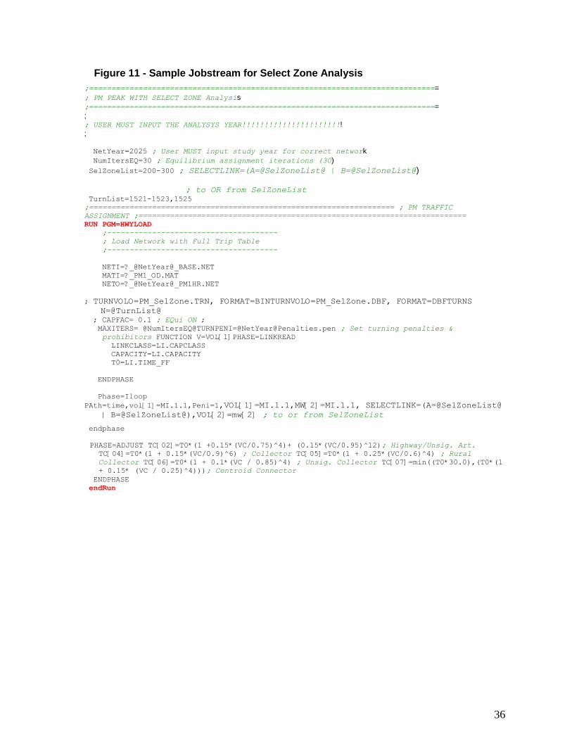
36
Figure 11 - Sample Jobstream for Select Zone Analysis
;==============================================================================
; PM PEAK WITH SELECT ZONE Analysis
;==============================================================================
; ; USER MUST INPUT THE ANALYSYS YEAR!!!!!!!!!!!!!!!!!!!!!!!
; NetYear=2025 ; User MUST input study year for correct network
NumItersEQ=30 ; Equilibrium assignment iterations (30)
SelZoneList=200-300 ; SELECTLINK=(A=@SelZoneList@ | B=@SelZoneList@)
; to OR from SelZoneList
TurnList=1521-1523,1525
;==================================================================== ; PM TRAFFIC
ASSIGNMENT ;=========================================================================
RUN PGM=HWYLOAD
;--------------------------------------
; Load Network with Full Trip Table
;--------------------------------------
NETI=?_@NetYear@_BASE.NET
MATI=?_PM1_OD.MAT
NETO=?_@NetYear@_PM1HR.NET
; TURNVOLO=PM_SelZone.TRN, FORMAT=BINTURNVOLO=PM_SelZone.DBF, FORMAT=DBFTURNS
N=@TurnList@
; CAPFAC= 0.1 ; EQui ON ;
MAXITERS= @NumItersEQ@TURNPENI=@[email protected] ; Set turning penalties &
prohibitors FUNCTION V=VOL[1]PHASE=LINKREAD
LINKCLASS=LI.CAPCLASS
CAPACITY=LI.CAPACITY
T0=LI.TIME_FF
ENDPHASE
Phase=Iloop
PAth=time,vol[1]=MI.1.1,Peni=1,VOL[1]=MI.1.1,MW[2]=MI.1.1, SELECTLINK=(A=@SelZoneList@
| B=@SelZoneList@),VOL[2]=mw[2] ; to or from SelZoneList
endphase
PHASE=ADJUST TC[02]=T0*(1 +0.15*(VC/0.75)^4)+ (0.15*(VC/0.95)^12); Highway/Unsig. Art.
TC[04]=T0*(1 + 0.15*(VC/0.9)^6) ; Collector TC[05]=T0*(1 + 0.25*(VC/0.6)^4) ; Rural
Collector TC[06]=T0*(1 + 0.1*(VC / 0.85)^4) ; Unsig. Collector TC[07]=min((T0*30.0),(T0*(1
+ 0.15* (VC / 0.25)^4))); Centroid Connector
ENDPHASE
endRun
37
8. ADJUSTMENT OF RESULTS
The traffic validation indicates that the StanCOG model provides a good overall estimation of
travel demand patterns in Stanislaus County. However, it is recommended that traffic forecasts
on specific road segments use an adjustment process that accounts for validation errors. Where
base year traffic counts are available, forecast traffic volumes are calculated based on the
increment between the base year and future year model results:
Adj. Forecast Volume = Base Year Count + (Model Forecast Volume - Base Year Model Volume)
An incremental adjustment is generally recommended instead of an adjustment based on ratios.
A ratio adjustment factor does not guarantee continuity of traffic volumes between adjacent road
segments, and can result in very large adjustments on low-volume links.
8.1 Turn Movements
The StanCOG model has been validated to replicate overall existing traffic volumes in Stanislaus
County. The model accurately represents overall traffic volumes on roads grouped by
classification or across regional screenlines. In many locations, the model also accurately
estimates traffic on specific road segments. It is likely that the model will not be accurate
enough in every location to reliably calculate level of service directly from model output.
However, a validated model will generate good estimates of changes in traffic volume in
response to changes in land use or road network assumptions. Therefore, it is recommended that
adjustments be applied to model results prior to traffic operations analysis.
The primary reference for traffic model volume adjustments is National Cooperative Highway
Research Program Report (NCHRP) 255: Highway Traffic Data for Urbanized Area Project
Planning and Design, 1982 (now out of print). Some of the simplified procedures described in
NCHRP 255 can be improved using current computer programs.
8.1.1 Link Volumes
There are two common procedures for adjusting link volumes from a model:
1. Increments (adjust traffic counts by increment from base year model to future year
model)
2. Growth Factors (adjust traffic counts by ratio of future year model to base year model)
It is recommended that link volumes from the TPPG model be adjusted based on the increment
method, for any link where traffic counts are available. Factors may be applied in locations
where forecasts are needed and traffic counts are not available.
Discussion of Factor Method
The growth factor or ratio method calculates the ratio of future model forecast volumes to base
year model volumes and applies the ratio to the base year traffic count. For example, a segment
of a given street may have a 2006 traffic count of 24,000 daily vehicles. The validated 1998 base
year model may estimate a 2005 volume of 19,500 (19% low) and a 2020 volume of 23,800
(lower than the 2005 count). The growth factor method would calculate an overall factor of
23,800/19,500 = 1.22. Applying the factor of 1.22 to the count of 24,000 would result in an
adjusted forecast of 29,280.
The factor method can generate very odd results when either the traffic count or base year model
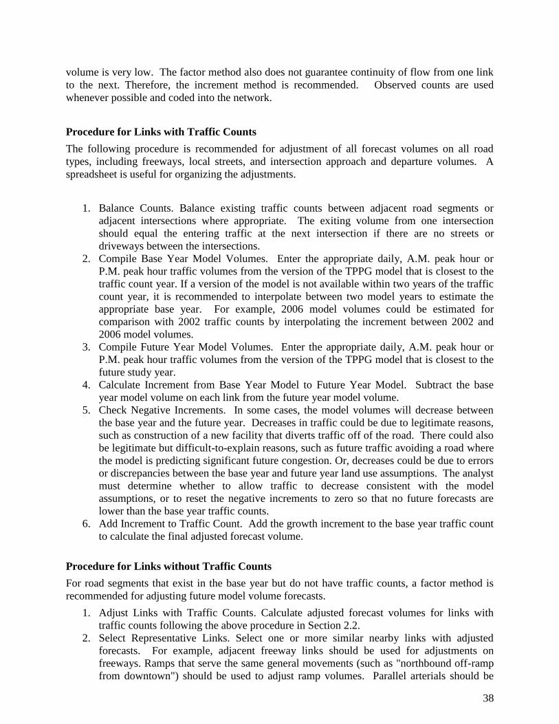
38
volume is very low. The factor method also does not guarantee continuity of flow from one link
to the next. Therefore, the increment method is recommended. Observed counts are used
whenever possible and coded into the network.
Procedure for Links with Traffic Counts
The following procedure is recommended for adjustment of all forecast volumes on all road
types, including freeways, local streets, and intersection approach and departure volumes. A
spreadsheet is useful for organizing the adjustments.
1. Balance Counts. Balance existing traffic counts between adjacent road segments or
adjacent intersections where appropriate. The exiting volume from one intersection
should equal the entering traffic at the next intersection if there are no streets or
driveways between the intersections.
2. Compile Base Year Model Volumes. Enter the appropriate daily, A.M. peak hour or
P.M. peak hour traffic volumes from the version of the TPPG model that is closest to the
traffic count year. If a version of the model is not available within two years of the traffic
count year, it is recommended to interpolate between two model years to estimate the
appropriate base year. For example, 2006 model volumes could be estimated for
comparison with 2002 traffic counts by interpolating the increment between 2002 and
2006 model volumes.
3. Compile Future Year Model Volumes. Enter the appropriate daily, A.M. peak hour or
P.M. peak hour traffic volumes from the version of the TPPG model that is closest to the
future study year.
4. Calculate Increment from Base Year Model to Future Year Model. Subtract the base
year model volume on each link from the future year model volume.
5. Check Negative Increments. In some cases, the model volumes will decrease between
the base year and the future year. Decreases in traffic could be due to legitimate reasons,
such as construction of a new facility that diverts traffic off of the road. There could also
be legitimate but difficult-to-explain reasons, such as future traffic avoiding a road where
the model is predicting significant future congestion. Or, decreases could be due to errors
or discrepancies between the base year and future year land use assumptions. The analyst
must determine whether to allow traffic to decrease consistent with the model
assumptions, or to reset the negative increments to zero so that no future forecasts are
lower than the base year traffic counts.
6. Add Increment to Traffic Count. Add the growth increment to the base year traffic count
to calculate the final adjusted forecast volume.
Procedure for Links without Traffic Counts
For road segments that exist in the base year but do not have traffic counts, a factor method is
recommended for adjusting future model volume forecasts.
1. Adjust Links with Traffic Counts. Calculate adjusted forecast volumes for links with
traffic counts following the above procedure in Section 2.2.
2. Select Representative Links. Select one or more similar nearby links with adjusted
forecasts. For example, adjacent freeway links should be used for adjustments on
freeways. Ramps that serve the same general movements (such as "northbound off-ramp
from downtown") should be used to adjust ramp volumes. Parallel arterials should be
39
used to adjust arterial segments. Calculate the adjustment factor on those nearby links as
the adjusted traffic volume divided by the unadjusted future year model volume.
3. Apply Adjustment Factor. Apply the average adjustment growth factor to the unadjusted
future year model volume on the link without traffic counts.
For future roads that do not exist in the base year, it would generally be appropriate to use
unadjusted model traffic volume forecasts.
8.1.2 Intersection Turn Volumes
It is possible to create a travel model that estimates accurate link volumes on a majority of
important road segments. However, it is very difficult to accurately estimate individual turn
movements. This is primarily due to the aggregation of land uses into transportation analysis
zones (TAZs), which means that the model cannot represent all of the individual paths that
drivers use to reach individual parcels and driveways. Therefore an adjustment process is
recommended. Growth factors derived from model approach volumes can be applied to count
approach volumes.
Procedure for Turn Movements
The procedure for intersection turn volumes is a two-step process. First, the link volumes
entering and exiting the intersection are adjusted as described above. Second, existing turn
movement counts are factored to match the adjusted entering and exiting volumes.
1. Adjust Link Volumes. Adjust the peak hour link volumes in and out of each leg of the
intersection (generally eight segments for a standard four-way intersection) using the
incremental adjustment process described in Section 2.2.
2. fFactor Turn Volumes. Factor the base year turn movement count at the intersection until
the total volumes in and out of each leg closely match the adjusted link volumes. A
common factoring algorithm is named after its creator, Furness. Computer applications of
the Furness procedure are available ("Turns32" on the Dowling Associates website,
www.dowlinginc.com, or the "LOS" program from TJKM Transportation Consultants,
"Estimate Turns from In/Out Volume" option) or simplified versions can be programmed
in spreadsheets.
3. Check Increments. Some of the factored turn movements may end up lower than the base
year traffic counts, due to large increases on certain exiting movements that divert traffic
away from other movements. The analyst must decide if the forecast turn movements
can decrease from the base year traffic counts, or if the forecast turn movements should
be reset to be no lower than the base year traffic counts.
Procedure for Movements without Traffic Counts
If a new road segment is added in the future, there will be no traffic counts available for
adjustment. The following procedure is recommended
1. Model Traffic Assignment. Assign future peak hour traffic using the Cube/Voyager
model and save turn movements at the selected intersections.
2. Intersection with Existing Road. If the new road will intersect an existing road, estimate
base year traffic counts and adjusted forecast link volumes on as many movements as
possible on the existing road at the new intersection based on traffic counts at adjacent
locations.
3. Substitute Model Volumes for Count. Substitute model-estimated turn movement

40
volumes as base year traffic counts for all turn movements to and from the new road.
4. Factor Turn Movements. Continue with the procedure described in Section 3.1.
Shortcut Procedure
The factoring procedure described in Section 3.1 will give the most representative results for
intersection turn movement forecasts based on growth on individual legs. However, there may be
times when the analyst may not have ready access to the adjustment software and needs a quick
assessment of intersection conditions. The following procedure is recommended for "shortcut"
analysis only:
1. Calculate Factors. Calculate the growth factors on each leg of the intersection as the
adjusted future year model volume (or unadjusted future year model volumes if
adjustments are not available) divided by the base year model volume (or base year
traffic count if the base year model is not available). The factor can be calculated based
on total two-way or directional one-way daily or peak hour model volumes.
2. Apply Factors. Apply the growth factor on each leg to the turn movement counts entering
from that leg;
OR
Calculate the growth factor for each turn movement as the average of the two growth
factors on the entering and exiting leg.
3. Check Results.
9. REPORTING THE RESULTS
There are a variety of ways to report the results of the StanCOG traffic assignment, including
screen graphics, plots and printed reports.
9.1 Viewing and Plotting Model Data
9.1.1 Network Project Files
Network project files are used by Viper to store various settings from the network window,
including:
The status and drawing order of the display layers
For each display layer
o File name
o Coordinate offset
o Coordinate scale
o Color specifications
o Selection criteria
Saved views
Saved polygons
Page setup information
Highway network attribute calculation information
Left-hand drive display option
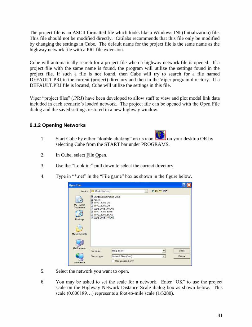
41
The project file is an ASCII formatted file which looks like a Windows INI (Initialization) file.
This file should not be modified directly. Citilabs recommends that this file only be modified
by changing the settings in Cube. The default name for the project file is the same name as the
highway network file with a PRJ file extension.
Cube will automatically search for a project file when a highway network file is opened. If a
project file with the same name is found, the program will utilize the settings found in the
project file. If such a file is not found, then Cube will try to search for a file named
DEFAULT.PRJ in the current (project) directory and then in the Viper program directory. If a
DEFAULT.PRJ file is located, Cube will utilize the settings in this file.
Viper “project files” (.PRJ) have been developed to allow staff to view and plot model link data
included in each scenario‟s loaded network. The project file can be opened with the Open File
dialog and the saved settings restored in a new highway window.
9.1.2 Opening Networks
1. Start Cube by either “double clicking” on its icon on your desktop OR by
selecting Cube from the START bar under PROGRAMS.
2. In Cube, select File Open.
3. Use the “Look in:” pull down to select the correct directory
4. Type in “*.net” in the “File name” box as shown in the figure below.
5. Select the network you want to open.
6. You may be asked to set the scale for a network. Enter “OK” to use the project
scale on the Highway Network Distance Scale dialog box as shown below. This
scale (0.000189…) represents a foot-to-mile scale (1/5280).
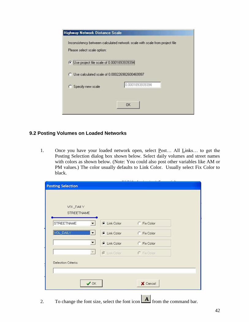
42
9.2 Posting Volumes on Loaded Networks
1. Once you have your loaded network open, select Post… All Links… to get the
Posting Selection dialog box shown below. Select daily volumes and street names
with colors as shown below. (Note: You could also post other variables like AM or
PM values.) The color usually defaults to Link Color. Usually select Fix Color to
black.
2. To change the font size, select the font icon from the command bar.

43
3. Select File… Printer Setup… to get your printer options. I usually select Portrait
for the full StanCOG model area and Landscape for zoomed in views. Note: These
do not be save in the Cube project files and must be reset when reopening a
network.
4. Select View… Resize to Plot Page… to set your view window so WYSIWYG
(what you see is what you get…).
5. Select View… Restore… to zoom in to any of the predefined window areas.
6. Select File… Print… to print to your defined printer or plotter.
10. THE FORECASTING PROCESS -TRIP GENERATION
The trip generation step quantifies the total magnitude of travel (person trips) generated in each
zone based upon land uses within the zone.
10.1 Trip Stratification
Trips are stratified by five trip purposes. The trip ends generated within any area are further
classified as either trip end productions or trip end attractions. The five trip purposes are
estimated separately and then later combined prior to assignment to the networks.
10.1.1 Trip Purposes
To derive more accurate projections of future travel behavior, the StanCOG model stratifies trip
ends by five trip purposes:
1. Home-Work trips are commute trips between residences and places of
employment, including both trips from home to work and from work to home.
2. Home-School trips are between residences and educational institutions.
3. Home-Shop trips are trips between residences and places of retail employment.
4. Home-Other trips account for all other trips which begin or end at home, and
include school trips, social trips and recreational trips.
5. Other-Work trips are trips between places of employment and places other than
home, such as driving to a restaurant during a lunch break, driving a delivery truck
away from the main office, or stopping at the gas station on the way home from
work.
6. Other-Other trips account for all other “non home based” trips, such as trips
between two other stores or long-distance truck trips.
Splitting the trips into purposes allows for a better understanding of the relationship between jobs
and housing, by separating commute trips. It also provides more control over the trip
distribution, since different types of trips involve different trip lengths. For a peak period model,
it is important to identify the differences in travel characteristics over the day.
10.1.2 Productions and Attractions
Consistent with conventional modeling practice, each one-way trip is defined as having two trip
ends in the trip generation process:

44
Trip Production. This is defined as the home end of any home-based trip, regardless of
whether the trip is directed to or from home. If neither end of the trip is a home (i.e.,
non-home based), it is defined as the origin end.
Trip Attraction. This is the non-home end (e.g., place of work, school or shopping) of a
home-based trip. If neither end of the trip is a home (i.e., it is a non-home based trip), the
trip attraction is defined as the destination end.
In other words, trip productions are generally home related while trip attractions are generally
related to place of work. For example, a typical commute from home to work in the morning and
then back home in the evening represents two separate one-way trips, and there are two trip ends
produced in the home zone and two trip ends attracted in the work zone.
10.2 Trip Generation Rates (Person Trips)
Trip generation rates (person trips) for the StanCOG peak period model were derived from the
2001 Caltrans Statewide Travel Survey (the most recent available at the time of this writing),
supplemented by information from previously developed models and knowledge about the
accuracy of travel surveys. Separate trip generation rates were derived for each land use cross
classification and employment category and for each trip purpose.
10.2.1 Household Trip Productions
A standard procedure for “cross-classification” trip generation would be to determine the average
trip rate for each of the six household categories. With a small survey sample size, this
procedure can result in zero or inconsistent rates for certain household categories. The StanCOG
model uses a “proportional smoothing” technique to determine the household rates. The
proportional smoothing technique calculates the average ratio of rates for single family versus
multiple family households, and the average ratios of rates for household size and auto
ownership categories. The ratios are then combined to determine the rates for each of the six
individual categories. These rates are substituted for zero values obtained from the survey and
show the cross-classified household trip generation rates for single family and multi family
households respectively.
10.2.2 Work-Other Trip Productions
The Caltrans Statewide Travel Survey can also provide some information on trips made by
surveyed workers. For each surveyed person, the work trip characteristics can be correlated to
their reported type of employment. These survey records were used to determine Work-Other
productions for each of the five types of employment in the StanCOG model.

45
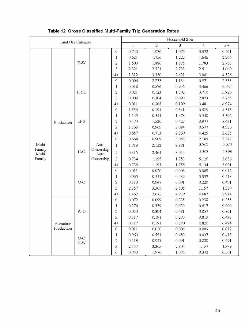
46

47
Table 13 Employment Trip Generation Rates
Land-Use Trip Purpose
H-W H-SC H-S H-O W-O O-O
Retail 1.73 4.89
Service 1.15 0.29
Educ Productions 1.15
Govt 1.15 2.01
Other 1.04
Retail 1.32 5.75 2.59 1.73 4.89
Service 1.32 3.45 1.15 0.29
Educ Attractions 1.32 20.70 1.15
Govt 1.32 1.90 1.15 2.01
Other 1.32 1.32 1.04
10.2.3 Trip Attractions
Home-Work attractions can be derived from the travel survey. Each surveyed person was also
asked about their type of employment. The average number of home-work commute trips for
each type of employment can be calculated from these survey records.
Home-Shop attractions were estimated by assuming that all Home-Shop trips are attracted to
retail employees. This is simplification, since some trips that people classify as Home-Shop may
be attracted to service or other employees (for example, a trip to the bank).
Trip attractions for other purposes are difficult to derive directly from limited travel survey data.
Work-Other trips and Other-Other trips are allocated based in order to fill out trip generation
rates for employment types using ITE rates as a guide with the end in mind that these trips
should be balanced and countywide totals by purpose should be reasonably well matched with
survey results.
The initial estimates of trip generation rates provided a close match with Stanislaus County totals
reported in the Caltrans Statewide Travel Survey. However, tests of the model indicated that
trips were underestimated, particularly along urban arterials and collectors.
It is assumed that the most likely trips to be under-reported in the travel survey would be
incidental trips, such as a trip from the grocery store to the laundry. These trips mostly fall into
the Other-Other category.
The Other-Other production and attraction rates for each employment type were estimated by
comparing the trip generation to standard vehicle trip generation rates in the ITE Trip Generation
Manual (Institute of Transportation Engineers, 7th
Edition,
2004). The model person trip generation rates were converted to vehicle trips using auto
occupancies for each trip purpose. The vehicle trip rates were compared for each employment
type. The Other-Other trip rates were increased so that the model trip generation rates would
replicate the ITE vehicle trip generation rates.
48
10.3 Cordon or “Gateway” Trips
There are two types of trips at the cordons or “gateways” of the TPPG model, through trips
(external-external or X-X) and external trips (external-internal, internal-external or I-X/X-I).
Through trips are trips that pass through the model area without stopping (e.g., a trip from San
Joaquin County to Merced). External trips have one end in Stanislaus County and one end
outside Stanislaus County (e.g., a trip from San Joaquin County). External trip assumptions are
shown in Appendix A. The external vehicle trips for each trip purpose are multiplied by the
appropriate average auto occupancy rate to convert them to person trips. Initial estimates of
productions and attractions at each gateway are adjusted to provide an overall balance of
gateway person-trip productions and attractions with internal person-trip productions and
attractions. These “gateway” trips are then distributed to the model zones along with the internal
model area trips. A gateway study will be carried out in 2010-11 and XX, IX and XI trips will
be based on 2010 origin-destination information.
10.3.1 Through Trips
The largest numbers of through trips pass through the county on SR 99. Daily 2006 vehicle
through trips were estimated for Stanislaus County based on actual counts at the gateways and
the proportion of trips considered to be through trips in the Caltrans Statewide Model. Future
through trips were factored at 1% compounded annually. Peak hour through trips were factored
based on peaking factors and directional factors on freeway gateways and adjusted during
calibration. A gateway study will be carried out in 2010-11 and XX, IX and XI trips will be
based on 2010 origin-destination information.
10.3.2 External Trips
External trips to and from Stanislaus County were estimated from 2006 traffic counts at the
cordon points. Through trips were subtracted from the traffic counts, leaving just the external
vehicle trips that have only one end in Stanislaus County. External trips (I-X and X-I) at each of
the gateways were split into the six trip purposes (home work, home-shop, home-other, other-
work, other-other) based on Stanislaus County averages.
10.4 Special Generators
Special generators are used to include trips from land uses that are not well represented by the
standard trip rates. In the TPPG model, special generators are used primarily to define Home-
Other trips attracted to recreational areas such as parks and golf courses. Typical vehicle trip
generation values were estimated for each of these recreational areas based on previous studies.
The vehicle trips are converted to person trips using
average auto occupancy rates. The special generator trips are then added to the appropriate
TAZs after trips are calculated using the standard household and employment trip generation
rates. ( shows the special generators used in the model.)

49
11. THE FORECASTING PROCESS -TRIP DISTRIBUTION
The trip distribution process estimates how many trips travel from one zone to another.
Consistent with many regional models across the country, the StanCOG model uses a method
known as the gravity model to estimate trips between zones based on the trip productions and
attractions in each zone and on factors that relate the likelihood of travel between zones to the
separation between the zones.
11.1 Description of Gravity Model
The gravity model follows the concept of Isaac Newton‟s Universal Law of Gravitation, which
states that the attractive force between two bodies is proportional to the product of their masses
and inversely proportional to the square of the distance between them. Similarly, zone-to-zone
trip interchanges in the gravity model are directly proportional to the relative attraction or
opportunity provided by each of the zones (productions and attractions) and inversely
proportional to the spatial separation between zones. Expressed mathematically, the gravity
model formula of trip distribution is:
T ij = P I * Aj F(t ij) K ij .
Sum x=1,n [AxF(t ij) Kij]
where: T ij = number of trips produced in zone i and attracted to zone j
P i = total number of trips produced in zone i
A j = attractions of zone j
t ij = travel time in minutes between zone i and zone j
F(t ij) = the friction factors between zone i and zone j
K ij = zone-to-zone adjustment factor
n = number of zones
The inputs to the gravity model include the person trip productions and attractions for each zone
(as defined earlier in the trip generation step), the zone-to-zone travel times, and friction factors
that define the effects of travel time. The zone-to-zone distributions are calculated separately for
each trip purpose.
11.2 Zone-To-Zone Travel Times
The travel time between each pair of zones is calculated by determining the shortest time path
along the coded road network between the two zones, and accumulating the travel time along
that path. The path building process produces a table (skim matrix) of travel times between each
pair of zones in the study area. The resulting table of zone-to-zone travel times is then used as an
input to the trip distribution analysis.
50
For this estimation, road travel times are used since the large majority of person-travel is on the
road system. Uncongested (free flow) travel times are used in the initial estimates of the trip
distribution, but travel times which reflect congestion levels are used for the final trip
distribution.
11.2.1 Intrazonal Travel Times
Intrazonal travel times represent the average travel time for trips that stay within a particular
zone. They are estimated based on 50 percent of the travel time to the nearest adjacent zone.
11.2.2 Terminal Times
Terminal times are also added to represent the average time to access one‟s vehicle at each end
of a trip. The StanCOG model assumes an average terminal time of one minute for most trips.
11.3 Friction Factors
The effects of spatial separation in the gravity model are represented empirically by “friction
factors” that express the effect that travel time exerts on the propensity for making a trip to a
given zone. Typically the probability for making a particular trip declines as the travel time
increases. For the StanCOG model, five sets of friction factors are used, with each set
corresponding to one of the five trip purposes. This accounts for the possibility that people may
be willing to drive a long distance to go to work, but only short distances for most shopping or
school trips.
11.4 Adjustment Factors
Adjustment Factors (“K factors”) can be used in gravity model trip distribution calculations
where travel time does not fully explain the attractiveness or unattractiveness of certain trips.
The adjustments are often used where bridges, other perceived travel barriers or special
socioeconomic factors (such as housing prices or campus housing areas) may distort the
distribution of trips between specific areas.
K-Factors are not used by default in the StanCOG model. The inclusion of K-factors may be
suitable for specific model applications but this should only be undertaken by advanced users.
12. THE FORECASTING PROCESS -TRIP ASSIGNMENT
In this step, zone-to-zone trips from the trip distribution step are assigned to the network. The
StanCOG model does not currently assign transit trips to a transit network.
12.1 Traffic Assignment
The StanCOG model uses a process known as “equilibrium” assignment to assign vehicles.
Vehicle trips are initially assigned to the road network using the all-or-nothing method, which
assumes that all drivers will use the fastest route without regard to congestion caused by other
vehicles. Travel times on the road network are recalculated based on the estimated level of
congestion, and trips are reassigned to paths based on the congested speeds. The process is
repeated for several iterations. After each iteration, some traffic is shifted to alternative routes
51
with competitive travel times. The equilibrium assignment method is intended to ultimately
assign traffic so that no driver can shift to an alternative route with a faster travel time. The
overall road system is considered to be at equilibrium at this point. The StanCOG model uses
eight iterations for each final traffic assignment.
12.1.1 Traffic Assignment Time Periods
The StanCOG model assigns traffic for daily traffic, the AM and PM peak hours and 22 hours in
the off peak. Peak hour traffic is derived from daily traffic and assigned after feedback (see
sections 7 and 8).
12.1.2 Congested Travel Speeds
The relationship of speed to congestion on a particular roadway is based on a set of curves which
are included in the traffic assignment model. The curves are based on the standard British Public
Roads Curve:
T = T(free Flow) * (1 + 0.15(VC/0.75)4
) BPR Speed Curve
For example, the curves may indicate that an arterial street with no congestion will operate at 35
miles per hour so that a segment of that street takes 60 seconds to traverse, while an arterial link
with a traffic volume equal to 90 percent of the capacity of the link will operate at about 27 miles
per hour and take 80 seconds to traverse.
Adjustment to this basic curve are made during validation and calibration. Adjusted curves are
employed for:
Rural Highways /Unsig. Arterials = T0*(1 +0.15*(VC/0.75)^4)+ (0.15*(VC/0.95)^12) Collectors = T0*(1 + 0.15*(VC/0.9)^6) Rural Collector = T0*(1 + 0.25*(VC/0.6)^4) Unsignalized Collector =T0*(1 + 0.1*(VC / 0.85)^4) Centroid Connector =min((T0*30.0),(T0*(1 + 0.15* (VC / 0.25)^4))) Class B Expressway =T0*(1 +0.15*(VC/0.75)^4+ 0.05*(VC/0.98)^6) Class C Expressway =T0*(1 +0.15*(VC/0.75)^4+ 0.05*(VC/0.98)^6)
Identical speed curves are used by the model for the daily and peak hour assignment
processes.
12.2 Pricing
The StanCOG travel model does not explicitly consider travel cost considerations. Travel costs
would include auto operating costs (fuel, insurance, repairs), parking costs, transit fares and tolls.
These cost factors become most important when the travel model is considering the trade-offs
between autos and other modes such as transit. If a mode choice analysis capability is added to
the StanCOG model, these cost parameters would be added at the appropriate analysis steps
52
13. THE FORECASTING PROCESS -FEEDBACK MECHANISMS
The StanCOG travel model includes a feedback loop that uses congested travel times as an input
to the trip distribution step. The feedback loop is intended to ensure that the congested travel
impedances (times) used for final traffic assignment and as input to the air quality analysis are
consistent with the travel impedances used throughout the model process.
In the StanCOG model, the feedback loop is considered to converge when the travel times that
result from the congested travel speeds after traffic assignment compare closely with the travel
times used as input to the trip distribution process.
13.1 StanCOG Model Feedback Loop
In an effort to meet all Transportation Conformity Rule modeling requirements as part of the
model integration, a full feedback loop process was implemented that iterates until it reaches a
set of convergence criteria. The convergence criteria are consistent with Transportation
Conformity Rule Section 93.12 (b)(1)(v).
13.1.1 Congested Travel Times
The initial trip distributions for all six trip purposes are calculated using uncongested (free-flow)
travel times on the road network. After the initial trip distribution and assignment, the congested
travel times calculated from the most recent daily traffic assignment are used as input to the trip
distribution and the distribution is rerun. The feedback loop convergence criteria are based on
convergence of the congested travel times.
13.1.2 Method of Successive Averages
In order to speed up the convergence of the feedback loop, an interpolation method is used. The
method of successive averages takes the latest set of congested travel times calculated from the
latest traffic assignments, and calculates a weighted average with the latest set of travel times
used as input to trip distribution. The weighting is based on the number of iterations. For
example, after the fourth pass through the feedback loop, the weighted average would be
calculated as one-quarter (0.25) times the latest set of congested travel times plus three-quarters
(0.75) times the previous set of congested travel times. This process is repeated until the
convergence criteria are met. The base year model currently converges in three loops.
13.1.3 Convergence Criteria
A set of convergence criteria were developed specifically for this model to ensure that the
congested travel speeds used as input to the air quality analysis are consistent with the travel
speeds used throughout the model process, as required by the Transportation Conformity Rule.
The congested travel speeds used as input to the air quality analysis come from the final traffic
assignments. The congested travel speeds used throughout the model process are those used as
input to the trip distribution step (and mode choice step if implemented). Therefore, the
convergence criteria are applied by comparing the congested travel speeds from the latest traffic
assignments with the congested travel speeds and times most recently used as input to trip
distribution. The inputs to trip distribution are calculated as a weighted average using the
method of successive averages as described above.

53
The StanCOG model feedback loop is considered to converge when:
1. Less than 5% of the origin-destination pairs have daily congested travel times that change
by more than 5% between iterations; and
2. The weighted average change in daily link traffic volumes is less than 5% between
iterations (the average percent change is weighted by the link volume).
If the first two criteria do not result in convergence after five iterations through the feedback
loop, it indicates that the network is very congested and the traffic assignments are oscillating
between one set of routes and another. The following criteria are then used after seven feedback
iterations:
3. The weighted average change in daily congested travel times between origin-destination
pairs is less than 5% between iterations (average weighted by number of origin-
destination trips); and
4. The weighted average change in daily congested travel times between origin-destination
pairs is less than 5% between iterations (average weighted by vehicle-miles of travel);
and
5. The weighted average change in daily link traffic volumes is less than 5% between
iterations (the average percent change is weighted by the link volume).
The second set of convergence criteria were found to close during tests even with very congested
future travel demands.
14. THE FORECASTING PROCESS -PEAKING FACTORS
The StanCOG peak period model has been set up to estimate travel demand during the AM, PM
and off peak 22 hours. Peak hour volumes are often required for capacity analysis and local
traffic studies.
14.1 Time-of-Day Factors
The AM peak hour period trips, the PM peak hour period trips and the off-peak 22hour period
trips are calculated by factoring the daily trips after trip distribution. The daily trips are factored
separately for each trip purpose as shown below in Table 14.
The time-of-day factors are based on information from the 2001 Caltrans travel survey
(Appendix C). Many travel models use time-of-day factors which are based on the start times of
each trip. The StanCOG model uses factors which are based on the “midpoint” of each trip,
looking at both the start and end times. This technique provides a more representative estimate
of the number of trips in progress during each time period. During model validation, the factors
were adjusted from the survey results. These peak hour factors should be reviewed and updated
when new peak hour traffic count and survey information is available.
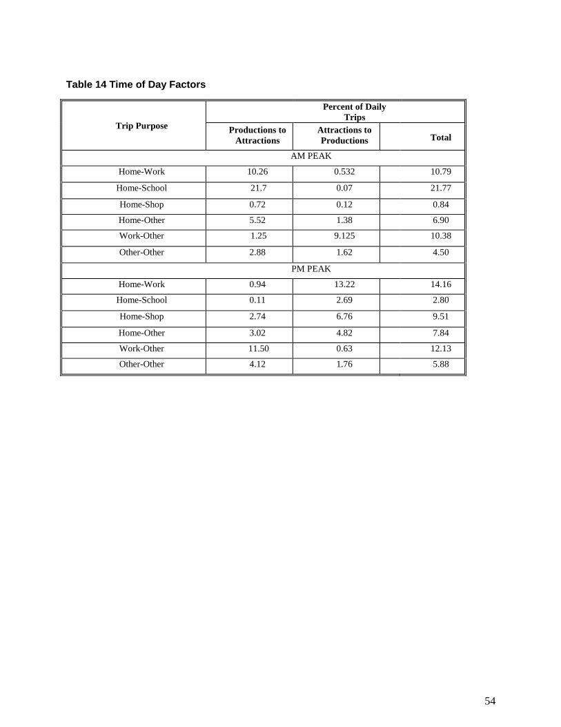
54
Table 14 Time of Day Factors
Trip Purpose
Percent of Daily
Trips
Productions to
Attractions
Attractions to
Productions
Total
AM PEAK
Home-Work 10.26 0.532 10.79
Home-School 21.7 0.07 21.77
Home-Shop 0.72 0.12 0.84
Home-Other 5.52 1.38 6.90
Work-Other 1.25 9.125 10.38
Other-Other 2.88 1.62 4.50
PM PEAK
Home-Work 0.94 13.22 14.16
Home-School 0.11 2.69 2.80
Home-Shop 2.74 6.76 9.51
Home-Other 3.02 4.82 7.84
Work-Other 11.50 0.63 12.13
Other-Other 4.12 1.76 5.88
55
APPENDIX A – VALIDATION
Model Validation
Model validation refers to comparing the model volumes to observed volumes. The following
sections describe how traffic data was collected and organized by screenlines and other
validation criteria along with the validation results. In 2009-10, StanCOG staff consolidated its
count data from its jurisdiction into a Traffic Monitoring Program for the benefit of its planning
partners.
Traffic Data
Traffic data for the year 2006 validation were obtained from a variety of sources, including
traffic counts provided by the StanCOG, Stanislaus County, and the Cities of Ceres, Hughson,
Modesto, Newman, Oakdale, Patterson, Riverbank, Turlock, and Waterford. Special
acknowledgement is also due to a number of private consultants including KdAnderson and
Associates, Omni Means Associates, Fehr and Peers and Associates, and TJKM and Associates
for providing data in electronic format. Traffic count data was collected by the California
Department of Transportation (Caltrans) at traffic monitoring locations on State highway
segments for validation and the CMP update.
Daily counts and peak hour counts were input directly into the network. Over 2,200 peak hour
580 daily traffic counts were entered. Duplicate counts were eliminated by replacing older
counts with newer counts and estimates of daily traffic were developed based on peak hour
traffic and the peaking factors obtained from the statewide travel survey. This resulted in 1,305
unique counts/count estimates for each of the AM, PM and daily traffic periods. The counts
utilized were included to allow the comparison of model output and observed traffic volumes
based on screenlines.
Summary
The StanCOG model estimates 2006 base year traffic on major regional facilities at a level of
accuracy sufficient to support evaluation of daily and peak hour traffic patterns for General Plan
analysis. With appropriate future year assumptions the model is ideal for use in traffic impact
analysis based on the Furness method of forecast estimation. The FHWA validation criteria are
fully satisfied. Twenty (20) screenlines were evaluated and all of these fall within an acceptable
range of accuracy.
Model Calibration Model calibration refers to adjustment to model inputs based on a comparison of model outputs
to observed conditions. During calibration, adjustments are made to the calibrated parameters
such as auto ownership, trip generation rates and distribution factors to more closely match
standard rates and published aggregate statistics in 2006.
56
Proposed Validation Criteria
The validation of the StanCOG regional transportation model is based on several criteria,
including the following:
Comparison to Vehicle Miles of Travel (VMT) from the Caltrans Highway
Performance Monitoring System (HPMS)
Comparison of model counts to observed traffic counts.
The percentage of links falling within the FHWA validation curve. The
FHWA suggested link-specific validation criteria is that 75% of freeway and
principal arterials fall below the validation criteria and 100% ofscreenlines
fall below the validation curve shown in Figure 1.
Use the Federal Highway Administration and Caltrans recommended error
limits for total error by functional classification (type of road) as a regionwide
validation :
o Freeways less than 7 percent error
o Principal Arterials less than 10 percent error
o Minor Arterials less than 15 percent error
o Collectors less than 25 percent error
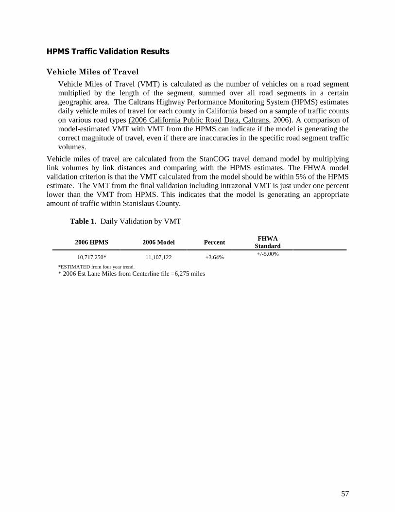
57
HPMS Traffic Validation Results
Vehicle Miles of Travel
Vehicle Miles of Travel (VMT) is calculated as the number of vehicles on a road segment
multiplied by the length of the segment, summed over all road segments in a certain
geographic area. The Caltrans Highway Performance Monitoring System (HPMS) estimates
daily vehicle miles of travel for each county in California based on a sample of traffic counts
on various road types (2006 California Public Road Data, Caltrans, 2006). A comparison of
model-estimated VMT with VMT from the HPMS can indicate if the model is generating the
correct magnitude of travel, even if there are inaccuracies in the specific road segment traffic
volumes.
Vehicle miles of travel are calculated from the StanCOG travel demand model by multiplying
link volumes by link distances and comparing with the HPMS estimates. The FHWA model
validation criterion is that the VMT calculated from the model should be within 5% of the HPMS
estimate. The VMT from the final validation including intrazonal VMT is just under one percent
lower than the VMT from HPMS. This indicates that the model is generating an appropriate
amount of traffic within Stanislaus County.
Table 1. Daily Validation by VMT
2006 HPMS 2006 Model Percent FHWA
Standard
10,717,250* 11,107,122 +3.64% +/-5.00%
*ESTIMATED from four year trend.
* 2006 Est Lane Miles from Centerline file =6,275 miles
58
FHWA Criteria
Total Volumes
The traffic counts and the model volumes are compared by facility type (Tables 2-4) and by the
volume range in which they are classified (Table 5). The comparison is made in terms of total
model volume compared to total traffic counts. A measure of variation is also provided, the
root mean square error (RMSE).
Facility Type. The Federal Highway Administration1 and Caltrans
2 recommend error limits for
total error by functional classification (type of road):
Freeways less than 7 percent error
Principal Arterials less than 10 percent error
Minor Arterials less than 15 percent error
Collectors less than 25 percent error
Frontage Roads less than 25 percent error
In the StanCOG transportation model, the “Principal Arterial” criterion is applied to
expressways and inter-urban highways, while the “Minor Arterial” criterion is applied to all local
arterial streets.
The 2006 traffic validation of the TPPG model meets the criteria for all facility types, for Daily,
AM and PM peak hour volumes. Key steps in achieving validation included:
The development of new capacity class: rural collector with a capacity of 950
vehicles per hour per lane (vphpl) for one directional lane and 850 vphpl for 2 or
more lanes,
The modification of speed curves based on multiple validation runs,
The adjustment of trip generation rates and review of land use inputs
Peak hour validation was further facilitated through the adjustment of peaking factors
across trip purposes.
Volume Range. Table B-1 lists the volume ranges which are recommended for the comparison
of daily traffic counts to model volumes by volume range. The final model validation meets the
FHWA criteria for all ten of the volume ranges. For those volume ranges, the total model
volume is within 1 percent of observed volumes
1 Federal Highway Administration, Calibration and Adjustment of System Planning Models, 1990 2 California Department of Transportation, Travel Forecasting Guidelines, 1992
59
Table 2: Daily Count/ Model Volume Comparison by Facility Type
Observed Model No. of Pct. Meets
Facility Type CapClass Criteria Counts Volumes Links Diff. Delta2 Diff. MSE %RMSE Criteria
Freeways 1 +/- 7% 3,353,981 3,565,716 77 211,735 4,065,125,092 6.3% 52,793,832 17% YES
Principal Arterials 2 +/- 10% 1,936,169 2,004,348 242 68,179 1,458,562,016 3.5% 6,027,116 31% YES
Arterials 3 +/- 15% 4,426,162 4,565,223 484 139,061 5,523,981,473 3.1% 11,413,185 37% YES
Collectors 4 +/- 25% 3,387,856 3,226,002 1,243 (161,854) 3,038,210,219 -4.8% 2,444,256 57% YES
All 13,104,168 13,361,289 2,046 257,121 14,085,878,801 2.0% 6,887,960 41%
Table 3: AM 1-Hour Count/ Model Volume Comparison by Facility Type
Observed Model No. of Pct. Meets
Facility Type CapClass Criteria Counts Volumes Links Diff. Delta2 Diff. MSE %RMSE Criteria
Freeways 1 +/- 7% 317,218 311,975 77 (5,243) 180,147,309 -1.7% 2,339,575 37% YES
Principal Arterials 2 +/- 10% 163,126 179,351 242 16,225 20,366,099 9.9% 84,157 43% YES
Arterials 3 +/- 15% 360,017 392,969 484 32,952 50,909,924 9.2% 105,186 44% YES
Collectors 4 +/- 25% 292,336 285,480 1,243 (6,856) 31,414,962 -2.3% 25,274 68% YES
All 1,132,697 1,169,775 2,046 37,078 282,838,294 3.3% 138,307 67%
Table 4: PM 1-Hour Count/ Model Volume Comparison by Facility Type
Observed Model No. of Pct. Meets
Facility Type CapClass Criteria Counts Volumes Links Diff. Delta2 Diff. MSE %RMSE Criteria
Freeways 1 +/- 7% 324,511 327,006 77 2,495 140,286,621 0.8% 1,821,904 32% YES
Principal Arterials 2 +/- 10% 175,845 187,083 242 11,238 18,747,352 6.4% 77,468 38% YES
Arterials 3 +/- 15% 422,993 407,730 484 (15,263) 58,222,589 -3.6% 120,295 40% YES
Collectors 4 +/- 25% 325,657 286,277 1,243 (39,380) 34,707,186 -12.1% 27,922 64% YES
All 1,249,006 1,208,096 2,046 (40,910) 251,963,748 -3.3% 123,210 57%
Table 5: Daily Count/ Model Volume Comparison by Volume Range
Observed Model No. of Pct.
From To Criteria Counts Volumes Links Diff. Delta2 Diff. MSE %RMSE Criteria
1 5,000 +/- 60% 2,723,150 2,989,344 1,298 266,194 3,670,058,809 9.8% 2,827,472 80% YES
5,000 10,000 +/- 55% 3,101,047 3,100,844 427 (203) 2,366,298,942 0.0% 5,541,684 32% YES
10,000 20,000 +/- 45% 3,778,352 3,686,881 285 (91,471) 4,165,882,101 -2.4% 14,617,130 29% YES
20,000 30,000 +/- 40% 744,948 686,026 34 (58,922) 379,245,862 -7.9% 11,154,290 15% YES
30,000 40,000 +/- 37% 417,096 436,353 12 19,257 579,288,784 4.6% 48,274,065 20% YES
40,000 50,000 +/- 34% 352,800 381,225 8 28,425 643,609,399 8.1% 80,451,175 20% YES
50,000 75,000 +/- 28% 2,280,081 2,419,819 38 139,738 2,522,818,996 6.1% 66,389,974 14% YES
Sum 13,397,474 13,700,492 2,102 303,018 14,327,202,894 2.3% 6,819,230 41%
Volume Range
60
Root Mean Square Error. The root mean square error (RMSE) is a statistical estimator that is
intended to represent the average percent error between an estimated value (such as a model
volume) and an observed value (such as a traffic count). The RMSE is calculated as:
n
∑(Ci −V
i )
2
RMSE = i=1
, where
n is the total number of links
Ci is the observed count for road i
Vi is the model volume for road i
i represents a road link link
The RMSE provides a measure of accuracy based on the statistical standard deviation. The
RMSE puts a greater emphasis on larger errors that may cancel each other out in the comparison
of total model volumes and traffic counts. The overall target daily RMSE is 40 percent, which is
met generally ranges. Generally on low volume roads RMSE will be relatively high as small
differences in absolute volume represent large increases in RMSE on low volume roads.
Similarly, peak hour RMSE is typically higher that daily RMSE.
Screenlines
Screenlines are imaginary lines, often along natural or man-made physical barriers (e.g., rivers,
railroad tracks) that ideally have a limited number of crossings. To the extent possible
screenlines should “cut” the entire study area, intercepting all travel across them, thereby
eliminating issues about individual route choice. Use of a system of screenlines allows
systematic comparison of total model estimated versus observed travel in different parts of the
model area. However, they do not ensure that traffic is being assigned to the correct routes
across each screenline. The study area includes 20 screenlines.
Screenline Validation
A comparison of model volumes to 2006 traffic counts across screenlines for the daily period is
presented based for 20 screenlines. The locations of these screenlines are shown on Figure 1.
The results of screenlines validation are presented in Table 6. Under both the two way and one
way comparisons all of the screenline estimates are satisfactory. Screenlines are broken down by
direction of travel. Northbound and Eastbound travel across screenlines are shown together on
Figure 3. Southbound and Westbound are shown on Figure 3. Figure 4 shows the maximum
tolerances under the FHWA criteria.
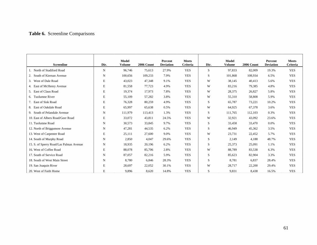
61
Table 6. Screenline Comparisons
Screenline Dir.
Model
Volume 2006 Count
Percent
Deviation
Meets
Criteria Dir.
Model
Volume 2006 Count
Percent
Deviation
Meets
Criteria
1. North of Stadiford Road N 96,746 75,613 27.9% YES S 97,833 82,009 19.3% YES
2. South of Kiernan Avenue N 100,656 109,233 7.9% YES S 101,868 108,934 6.5% YES
3. West of Dale Road E 43,023 47,348 9.1% YES W 38,145 40,413 5.6% YES
4. East of McHenry Avenue E 81,558 77,723 4.9% YES W 83,216 79,385 4.8% YES
5. East of Claus Road E 19,374 17,973 7.8% YES W 28,375 26,827 5.8% YES
6. Tuolumne River E 55,109 57,282 3.8% YES W 55,310 58,808 5.9% YES
7. East of Sisk Road E 76,328 80,259 4.9% YES S 65,787 73,221 10.2% YES
8. East of Oakdale Road E 65,997 65,638 0.5% YES W 64,925 67,378 3.6% YES
9. South of Pelandale Avenue N 111,979 113,413 1.3% YES S 111,765 112,103 0.3% YES
10. East of Albers Road/Geer Road E 33,072 43,811 24.5% YES W 32,921 43,092 23.6% YES
11. Tuolumne Road N 30,573 33,845 9.7% YES S 33,458 33,470 0.0% YES
12. North of Briggsmore Avenue N 47,281 44,535 6.2% YES S 46,949 45,362 3.5% YES
13. West of Carpenter Road E 25,111 27,600 9.0% YES W 23,731 22,452 5.7% YES
14. South of Murphy Road N 2,850 4,047 29.6% YES S 2,149 4,188 48.7% YES
15. S. of Sperry Road/Las Palmas Avenue N 18,935 20,196 6.2% YES S 25,373 25,091 1.1% YES
16. West of Coffee Road E 88,078 85,706 2.8% YES W 88,789 83,538 6.3% YES
17. South of Service Road N 87,057 82,216 5.9% YES S 85,623 82,904 3.3% YES
18. South of West Main Street N 8,780 6,846 28.3% YES S 8,781 6,837 28.4% YES
19. San Joaquin River E 28,697 22,052 30.1% YES W 28,717 22,200 29.4% YES
20. West of Faith Home E 9,896 8,620 14.8% YES S 9,831 8,438 16.5% YES
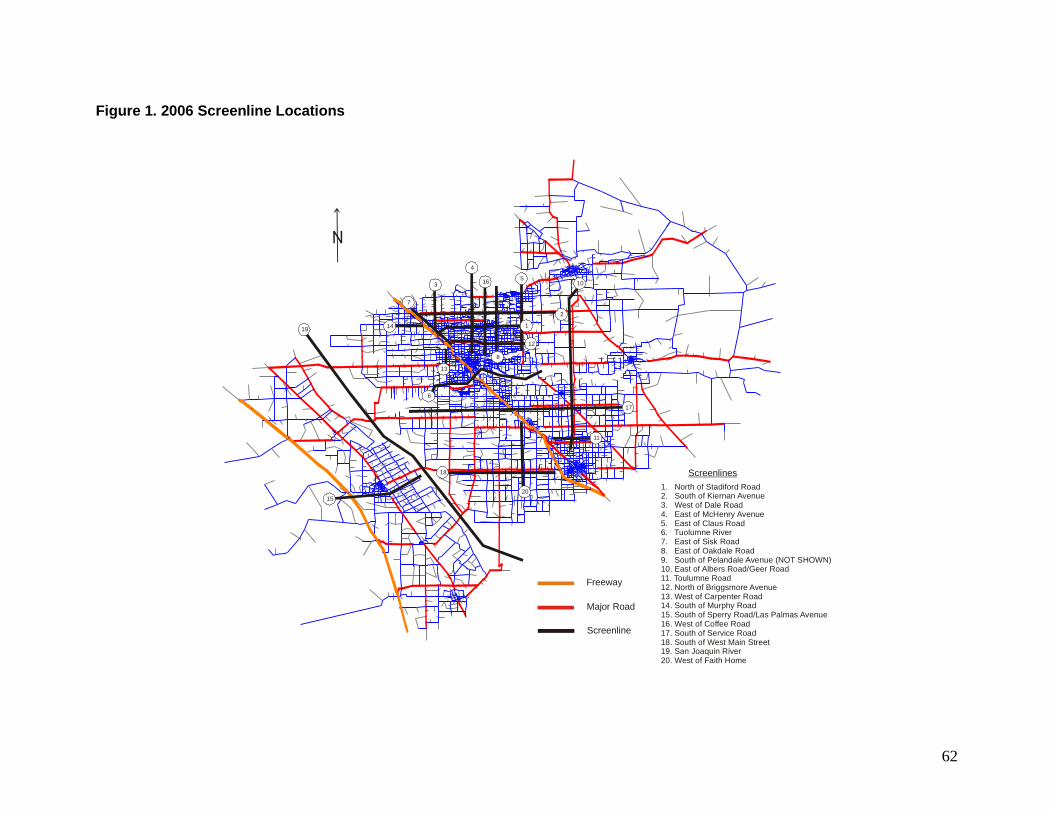
62
Figure 1. 2006 Screenline Locations
2
3
20
13
10
14
15
16
17
19
18
11
5
6
7
8
4
1
12
Freeway
Major Road
Screenline
1. North of Stadiford Road2. South of Kiernan Avenue3. West of Dale Road4. East of McHenry Avenue5. East of Claus Road6. Tuolumne River7. East of Sisk Road8. East of Oakdale Road9. South of Pelandale Avenue (NOT SHOWN)10. East of Albers Road/Geer Road11. Toulumne Road12. North of Briggsmore Avenue13. West of Carpenter Road 14. South of Murphy Road15. South of Sperry Road/Las Palmas Avenue16. West of Coffee Road17. South of Service Road18. South of West Main Street19. San Joaquin River20. West of Faith Home
Screenlines
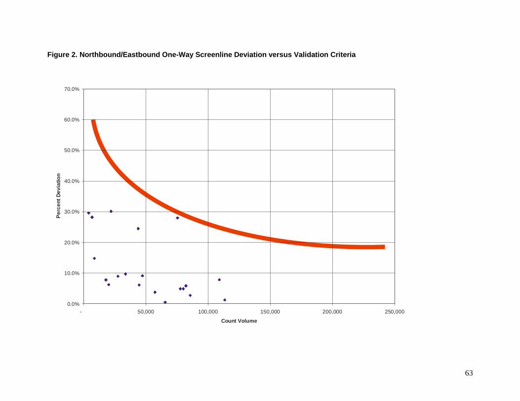
63
Figure 2. Northbound/Eastbound One-Way Screenline Deviation versus Validation Criteria
0.0%
10.0%
20.0%
30.0%
40.0%
50.0%
60.0%
70.0%
- 50,000 100,000 150,000 200,000 250,000
Count Volume
Pe
rce
nt
De
via
tio
n
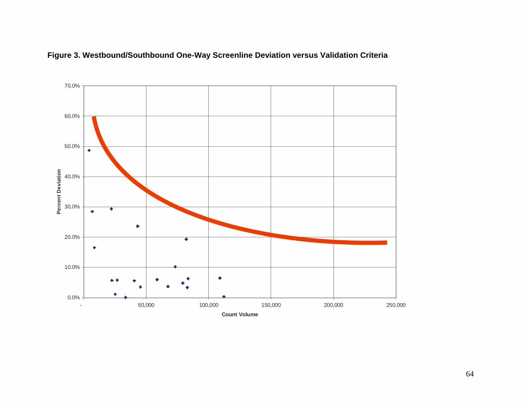
64
Figure 3. Westbound/Southbound One-Way Screenline Deviation versus Validation Criteria
0.0%
10.0%
20.0%
30.0%
40.0%
50.0%
60.0%
70.0%
- 50,000 100,000 150,000 200,000 250,000
Count Volume
Pe
rcen
tD
evia
tio
n
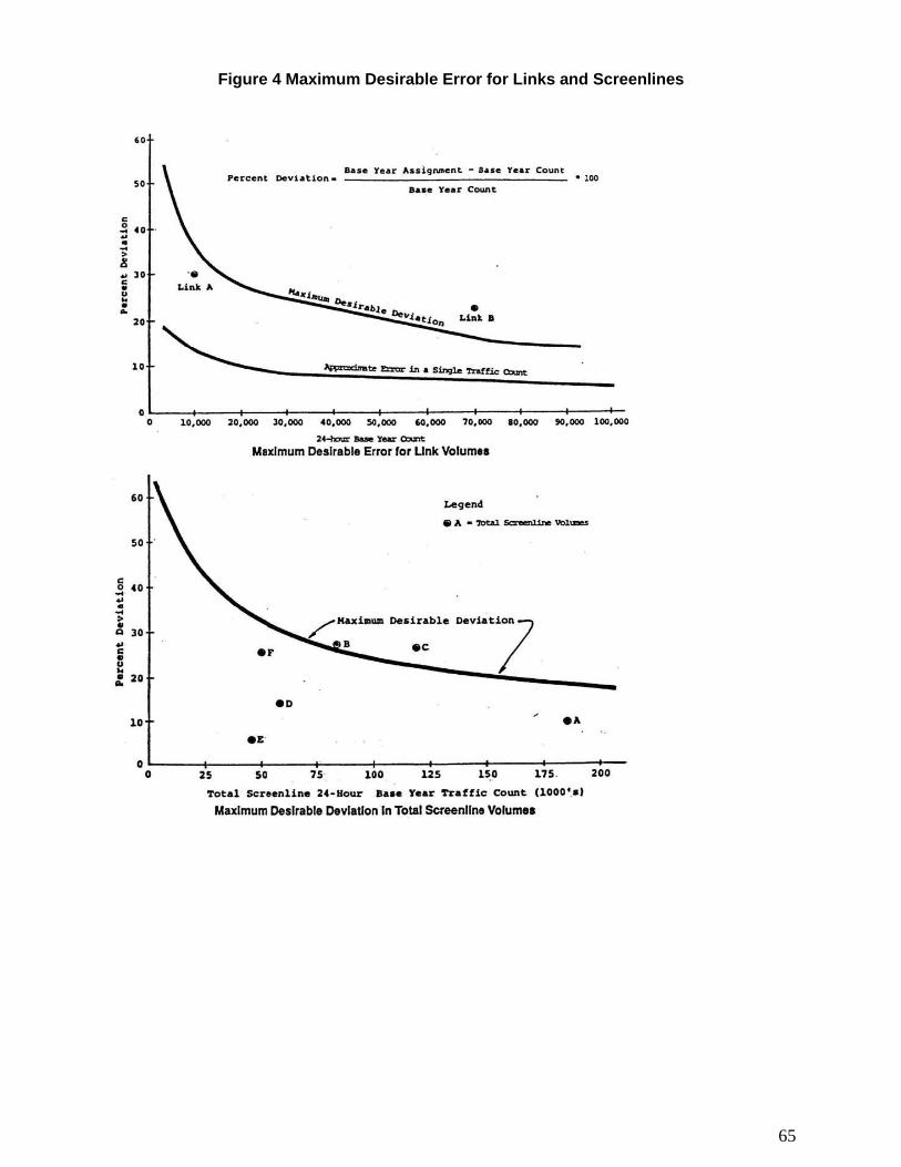
65
Figure 4 Maximum Desirable Error for Links and Screenlines

66
Appendix B Through Trips and Trips In and Out of the Region and Percent by Purpose
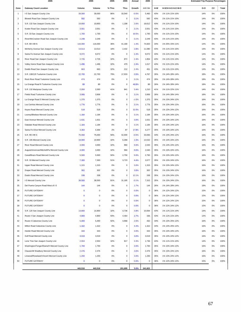
67
2005 2005 2005 2005 Annual 2005
Estimated Trip Purpose Percentages
Zone Gateway Count Location Volume Volume % Thru Thru Growth I-X / X-I H-W H-SCH H-S H-O W-O O-O CV Total
1 I-5 San Joaquin County Line 39,000 39,000 86% 33,540 -0.5% 5,460 43% 1% 11% 21% 10% 14% 0% 100%
2 Blewett Road San Joaquin County Line 592 592 0% 0 3.1% 592 43% 1% 11% 21% 10% 14% 0% 100%
3 S.R. 132 San Joaquin County Line 19,800 19,800 6% 1,188 2.6% 18,612 43% 1% 11% 21% 10% 14% 0% 100%
4 Koster Road San Joaquin County Line 3,551 3,551 0% 0 3.1% 3,551 43% 1% 11% 21% 10% 14% 0% 100%
5 S.R. 33 San Joaquin County Line 1,700 1,700 0% 0 19.5% 1,700 43% 1% 11% 21% 10% 14% 0% 100%
6 River/McCracken Road San Joaquin County Line 2,249 2,249 0% 0 3.1% 2,249 43% 1% 11% 21% 10% 14% 0% 100%
7 S.R. 99 I-99 N 116,000 116,000 36% 41,180 1.4% 74,820 34% 1% 25% 15% 11% 14% 0% 100%
8 McHenry Avenue San Joaquin County Line 13,513 13,513 18% 2,432 2.8% 11,080 43% 1% 11% 21% 10% 14% 0% 100%
9 Santa Fe Avenue San Joaquin County Line 9,072 9,072 0% 0 2.4% 9,072 43% 1% 11% 21% 10% 14% 0% 100%
10 River Road San Joaquin County Line 2,726 2,726 32% 872 2.4% 1,854 43% 1% 11% 21% 10% 14% 0% 100%
11 Valley Home Road San Joaquin County Line 1,496 1,496 32% 479 2.4% 1,017 43% 1% 11% 21% 10% 14% 0% 100%
12 Dodds Road San Joaquin County Line 663 663 32% 212 2.4% 451 43% 1% 11% 21% 10% 14% 0% 100%
13 S.R. 108/120 Tuolumne County Line 22,700 22,700 79% 17,933 0.5% 4,767 26% 1% 14% 28% 14% 18% 0% 100%
14 Rock River Road Tuolumne County Line 474 474 0% 0 3.1% 474 26% 1% 14% 28% 14% 18% 0% 100%
15 La Grange Road N Tuolumne County Line 89 89 0% 0 48.8% 89 26% 1% 14% 28% 14% 18% 0% 100%
16 S.R. 132 Mariposa County Line 2,050 2,050 41% 841 3.4% 1,210 41% 1% 11% 22% 11% 14% 0% 100%
17 Fields Road Tuolumne County Line 3,906 3,906 0% 0 3.1% 3,906 26% 1% 14% 28% 14% 18% 0% 100%
18 La Grange Road S Merced County Line 1,370 1,370 0% 0 -1.5% 1,370 35% 1% 13% 24% 12% 16% 0% 100%
19 Los Cerritos Merced County Line 1,776 1,776 0% 0 3.1% 1,776 35% 1% 13% 24% 12% 16% 0% 100%
20 Keyes Road Merced County Line 518 518 0% 0 32.0% 518 35% 1% 13% 24% 12% 16% 0% 100%
21 Looney/Bledsoe Merced County Line 1,184 1,184 0% 0 3.1% 1,184 35% 1% 13% 24% 12% 16% 0% 100%
22 East Avenue Merced County Line 1,631 1,631 0% 0 3.0% 1,631 35% 1% 13% 24% 12% 16% 0% 100%
23 Oakdale Road Merced County Line 1,184 1,184 0% 0 3.1% 1,184 35% 1% 13% 24% 12% 16% 0% 100%
24 Santa Fe Drive Merced County Line 4,364 4,364 2% 87 17.8% 4,277 35% 1% 13% 24% 12% 16% 0% 100%
25 S.R. 99 I-99 S 75,000 75,000 56% 42,000 -0.5% 33,000 34% 1% 13% 25% 12% 16% 0% 100%
26 S.R. 165 Merced County Line 19,900 19,900 32% 6,368 2.3% 13,532 35% 1% 13% 24% 12% 16% 0% 100%
27 River Road Merced County Line 3,000 3,000 32% 960 9.0% 2,040 35% 1% 13% 24% 12% 16% 0% 100%
28 August/American/Mitchell/Fa Merced County Line 3,000 3,000 32% 960 9.0% 2,040 35% 1% 13% 24% 12% 16% 0% 100%
29 Canal/Brazo Road Merced County Line 5,500 5,500 50% 2,750 9.0% 2,750 35% 1% 13% 24% 12% 16% 0% 100%
30 S.R. 33 Merced County Line 7,300 7,300 51% 3,723 4.4% 3,577 35% 1% 13% 24% 12% 16% 0% 100%
31 Upper Road Merced County Line 1,315 1,315 0% 0 3.0% 1,315 35% 1% 13% 24% 12% 16% 0% 100%
32 Draper Road Merced County Line 302 302 0% 0 3.0% 302 35% 1% 13% 24% 12% 16% 0% 100%
33 Eastin Road Merced County Line 338 338 0% 0 12.1% 338 35% 1% 13% 24% 12% 16% 0% 100%
34 I-5 Merced County Line 38,500 38,500 81% 31,185 -0.1% 7,315 35% 1% 13% 24% 12% 16% 0% 100%
35 Del Puerto Canyon Road West of I-5 144 144 0% 0 1.7% 144 26% 1% 14% 28% 14% 18% 0% 100%
36 FUTURE GATEWAY 0 0 0% 0 0.0% 0 36% 1% 12% 24% 12% 15% 0% 100%
37 FUTURE GATEWAY 0 0 0% 0 0.0% 0 36% 1% 12% 24% 12% 15% 0% 100%
38 FUTURE GATEWAY 0 0 0% 0 0.0% 0 36% 1% 12% 24% 12% 15% 0% 100%
39 FUTURE GATEWAY 0 0 0% 0 0.0% 0 36% 1% 12% 24% 12% 15% 0% 100%
40 S.R. 120 San Joaquin County Line 14,800 14,800 32% 4,736 3.8% 10,064 43% 1% 11% 21% 10% 14% 0% 100%
41 Route 4 San Joaquin County Line 4,800 4,800 93% 4,464 2.7% 336 43% 1% 11% 21% 10% 14% 0% 100%
42 Route 4 Calaveras County Line 5,400 5,400 92% 4,968 2.6% 432 34% 1% 13% 25% 12% 16% 0% 100%
43 Milton Road Calaveras County Line 1,322 1,322 0% 0 4.4% 1,322 34% 1% 13% 25% 12% 16% 0% 100%
44 Harder Road Merced County Line 343 343 0% 0 3.0% 343 35% 1% 13% 24% 12% 16% 0% 100%
45 Golf Road Merced County Line 3,019 3,019 0% 0 3.0% 3,019 35% 1% 13% 24% 12% 16% 0% 100%
46 Lone Tree San Joaquin County Line 2,553 2,553 32% 817 3.3% 1,736 43% 1% 11% 21% 10% 14% 0% 100%
47 Washington/Tenger/Elaine/H Merced County Line 1,700 1,700 0% 0 3.0% 1,700 35% 1% 13% 24% 12% 16% 0% 100%
48 Clausen/W Bradbury Merced County Line 2,476 2,476 0% 0 3.0% 2,476 35% 1% 13% 24% 12% 16% 0% 100%
49 Linwood/Roselawn/Vincent Merced County Line 1,200 1,200 0% 0 3.0% 1,200 35% 1% 13% 24% 12% 16% 0% 100%
50 FUTURE GATEWAY 0 0 0% 0 0.0% 0 36% 1% 12% 24% 12% 15% 0% 100%
443,518 443,518 201,695 5.0% 241,823