Embed Size (px)
Citation preview
Staggered and Non-Staggered
Time-Domain Meshless Radial Point
Interpolation Method in
Electromagnetics
by
Zahra Shaterian
B. Eng. (Electrical and Electronic),Amirkabir University of Technology, Iran, 2004
M. Eng. (Electrical and Electronic),K. N. Toosi University of Technology, Iran, 2008
Thesis submitted for the degree of
Doctor of Philosophy
in
Electrical and Electronic Engineering,
Faculty of Engineering, Computer and Mathematical Sciences
The University of Adelaide, Australia
2015

Supervisors:
Prof Christophe Fumeaux, School of Electrical & Electronic Engineering
Dr Thomas Kaufmann, School of Electrical & Electronic Engineering
© 2015
Zahra Shaterian
All Rights Reserved

To my parents
and my husband, Ali
with all my love.

Page iv
Contents
Contents v
Abstract ix
Statement of Originality xi
Acknowledgment xiii
Thesis Conventions xv
Publications xvii
List of Figures xxi
List of Tables xxv
Chapter 1. Introduction 1
1.1 Introduction . . . . . . . . . . . . . . . . . . . . . . . . . . . . . . . . . . . 2
1.2 Why Meshless Methods . . . . . . . . . . . . . . . . . . . . . . . . . . . . 3
1.3 Definition of Meshless Methods . . . . . . . . . . . . . . . . . . . . . . . . 4
1.4 Objectives of the Thesis . . . . . . . . . . . . . . . . . . . . . . . . . . . . . 4
1.5 Statement of Original Contribution . . . . . . . . . . . . . . . . . . . . . . 6
1.5.1 Staggered Meshless RPIM . . . . . . . . . . . . . . . . . . . . . . . 6
1.5.2 Non-Staggered Meshless RPIM . . . . . . . . . . . . . . . . . . . . 8
1.6 Overview of the Thesis . . . . . . . . . . . . . . . . . . . . . . . . . . . . . 10
Chapter 2. Overview of Mesh-based and Meshless Methods 13
2.1 Introduction . . . . . . . . . . . . . . . . . . . . . . . . . . . . . . . . . . . 14
2.2 Mesh-based Methods . . . . . . . . . . . . . . . . . . . . . . . . . . . . . . 14
2.2.1 Finite-Difference Time-Domain (FDTD) . . . . . . . . . . . . . . . 15
2.2.2 Finite Element Method (FEM) . . . . . . . . . . . . . . . . . . . . . 20
Page v
Contents
2.2.3 Limitations of Mesh-based Methods . . . . . . . . . . . . . . . . . 27
2.3 Meshless Methods . . . . . . . . . . . . . . . . . . . . . . . . . . . . . . . 27
2.3.1 Historical Overview . . . . . . . . . . . . . . . . . . . . . . . . . . 28
2.3.2 Main Steps in Meshless Methods . . . . . . . . . . . . . . . . . . . 28
2.3.3 Classification of Meshless Methods . . . . . . . . . . . . . . . . . 30
2.3.4 Meshless Methods with Different Shape Functions . . . . . . . . . 33
2.4 Summary . . . . . . . . . . . . . . . . . . . . . . . . . . . . . . . . . . . . . 39
Chapter 3. Radial Point Interpolation Method 41
3.1 Introduction . . . . . . . . . . . . . . . . . . . . . . . . . . . . . . . . . . . 42
3.2 Interpolation Method . . . . . . . . . . . . . . . . . . . . . . . . . . . . . . 42
3.2.1 Global Basis Functions . . . . . . . . . . . . . . . . . . . . . . . . . 43
3.2.2 Local Basis Functions . . . . . . . . . . . . . . . . . . . . . . . . . . 45
3.3 Different Radial Basis Functions (RBFs) . . . . . . . . . . . . . . . . . . . 47
3.3.1 Gaussian and Wendland Basis Functions . . . . . . . . . . . . . . 47
3.3.2 Comparing Gaussian and Wendland Basis Functions . . . . . . . 49
3.4 Conclusion . . . . . . . . . . . . . . . . . . . . . . . . . . . . . . . . . . . . 53
Chapter 4. Staggered Meshless RPIM 55
4.1 Staggered Meshless RPIM in Electromagnetics . . . . . . . . . . . . . . . 56
4.1.1 Time Discretization . . . . . . . . . . . . . . . . . . . . . . . . . . . 56
4.1.2 Space Discretization . . . . . . . . . . . . . . . . . . . . . . . . . . 57
4.1.3 Update Equations . . . . . . . . . . . . . . . . . . . . . . . . . . . . 60
4.2 Domain Truncation . . . . . . . . . . . . . . . . . . . . . . . . . . . . . . . 61
4.3 Uniaxial Perfectly Matched Layer (UPML) . . . . . . . . . . . . . . . . . . 64
4.3.1 Formulation of the UPML . . . . . . . . . . . . . . . . . . . . . . . 64
4.3.2 Late-Time Instability in UPML . . . . . . . . . . . . . . . . . . . . 71
4.4 Numerical Examples for the Staggered Meshless RPIM . . . . . . . . . . 75
4.4.1 Impact of Different Node Distributions . . . . . . . . . . . . . . . 75
4.4.2 Diplexer . . . . . . . . . . . . . . . . . . . . . . . . . . . . . . . . . 81
4.4.3 Scattering From a Conducting Sphere . . . . . . . . . . . . . . . . 83
4.5 Conclusion . . . . . . . . . . . . . . . . . . . . . . . . . . . . . . . . . . . . 90
Page vi
Contents
Chapter 5. Non-Staggered Meshless RPIM: Vector Potential Technique 95
5.1 Introduction . . . . . . . . . . . . . . . . . . . . . . . . . . . . . . . . . . . 96
5.2 Maxwell’s Equations: The Vector and Scalar Potentials . . . . . . . . . . 97
5.3 Magnetic Vector Potential . . . . . . . . . . . . . . . . . . . . . . . . . . . 98
5.4 Update Equations for A . . . . . . . . . . . . . . . . . . . . . . . . . . . . 100
5.4.1 Cartesian Coordinates . . . . . . . . . . . . . . . . . . . . . . . . . 100
5.4.2 Polar Coordinates . . . . . . . . . . . . . . . . . . . . . . . . . . . . 101
5.5 Perfect Electric Boundary Conditions for A . . . . . . . . . . . . . . . . . 102
5.5.1 Cartesian Coordinates . . . . . . . . . . . . . . . . . . . . . . . . . 102
5.5.2 Polar Coordinates . . . . . . . . . . . . . . . . . . . . . . . . . . . . 102
5.6 Perfectly Matched Layer (PML) for A . . . . . . . . . . . . . . . . . . . . 104
5.6.1 Hybridization of Staggered and Non-Staggered Meshless RPIM . 107
5.6.2 Numerical Results . . . . . . . . . . . . . . . . . . . . . . . . . . . 109
5.7 Numerical Examples for the Non-Staggered Meshless RPIM . . . . . . . 111
5.7.1 Parallel Plate Waveguide, TE1 Mode . . . . . . . . . . . . . . . . . 112
5.7.2 Iris Filter . . . . . . . . . . . . . . . . . . . . . . . . . . . . . . . . . 115
5.7.3 Tilted Parallel Plate Waveguide with TEM Mode . . . . . . . . . . 119
5.7.4 Parallel Plate Waveguide Bend with TEM Mode . . . . . . . . . . 120
5.7.5 Square Loop Antenna in 3D . . . . . . . . . . . . . . . . . . . . . . 122
5.8 Conclusion . . . . . . . . . . . . . . . . . . . . . . . . . . . . . . . . . . . . 123
Chapter 6. Comparing Staggered and Non-Staggered Meshless RPIM 127
6.1 Introduction . . . . . . . . . . . . . . . . . . . . . . . . . . . . . . . . . . . 128
6.2 Staggered Meshless RPIM . . . . . . . . . . . . . . . . . . . . . . . . . . . 129
6.3 Non-Staggered Meshless RPIM . . . . . . . . . . . . . . . . . . . . . . . . 130
6.4 Numerical Results . . . . . . . . . . . . . . . . . . . . . . . . . . . . . . . . 131
6.5 Conclusion . . . . . . . . . . . . . . . . . . . . . . . . . . . . . . . . . . . . 134
Chapter 7. Conclusion and Future Work 137
7.1 Part I: Staggered Meshless RPIM . . . . . . . . . . . . . . . . . . . . . . . 138
7.1.1 Summary of Original Contributions . . . . . . . . . . . . . . . . . 138
Page vii
Contents
7.1.2 Future Work . . . . . . . . . . . . . . . . . . . . . . . . . . . . . . . 140
7.2 Part II: Non-Staggered Meshless RPIM . . . . . . . . . . . . . . . . . . . . 140
7.2.1 Summary of Original Contributions . . . . . . . . . . . . . . . . . 140
7.2.2 Future Work . . . . . . . . . . . . . . . . . . . . . . . . . . . . . . . 142
Appendix A. Scattering from a Conducting Sphere: Theoretical Solution 145
Appendix B. Useful Identities in Cylindrical Coordinate System 149
Appendix C. Staggered Backward-Differentiation Time Integrators 151
Bibliography 153
Acronyms 165
Biography 167
Page viii
Abstract
Meshless methods have gained attention recently as a new class of numerical meth-
ods for the solution of partial differential equations in various disciplines of computa-
tional engineering. This class of methods offers several promising features compared
to mesh-based approaches. The principle of domain discretization with arbitrary node
distributions allows accurate modeling of complex geometries with fine details. More-
over, an elaborate and time-consuming re-meshing in the grid-based methods can be
replaced in meshless counterparts by an adaptive node refinement during the simula-
tion. This can be exploited to enhance solution accuracy or in optimization procedures.
In this thesis, the meshless Radial Point Interpolation Method (RPIM) is investigated
for application in time-domain computational electromagnetics. The numerical algo-
rithm is based on a combination of locally defined radial and polynomial basis func-
tions and yields a highly accurate local interpolation of field values and associated
derivatives based on the values at close neighboring positions. These interpolated par-
tial derivatives are used to solve the partial differential equations.
The thesis is firstly focused on the staggered meshless RPIM. The classical implemen-
tation of the staggered meshless RPIM in electromagnetics using the first-order Max-
well’s curl equations is described and the update equations for the staggered electric
and magnetic fields are shown. To enhance the capability of the algorithm, a novel
implementation of the Uniaxial Perfectly Matched Layer (UPML) is introduced. It is
shown however that UPML has intrinsically a long-time instability. Therefore, to avoid
this instability two loss terms are introduced, which are added to the update equations
in the UPML region after almost all the energy from the computational domain is ab-
sorbed. Various capabilities of the meshless method are then validated through differ-
ent numerical examples using staggered node arrangements in the staggered meshless
RPIM. However, the generation of a dual node distribution can be computationally
costly and restricts the freedom of node positions, which might reduce the potential
advantages of the scheme.
To overcome this challenge, the thesis next proposes a novel non-staggered algorithm
for the meshless RPIM based on a magnetic vector potential technique. In this method
instead of solving Maxwell’s curl equations for the electric and magnetic fields, the
Page ix
Abstract
wave equation for the magnetic vector potential is solved. Therefore, a single set of
nodes can be used to discretize the computational domain. Importantly in the pro-
posed implementation, solving the second-order vector potential wave equation in-
trinsically enforces the divergence-free property of the electric and magnetic fields and
the computational effort associated with the generation of a dual node distribution is
avoided. In this part of the thesis, a hybrid algorithm is further proposed to implement
staggered perfectly matched layers in the non-staggered RPIM framework. The prop-
erties of the proposed non-staggered RPIM are evaluated through several numerical
examples both in 2D and 3D implementations.
In the last part of the thesis, the staggered and non-staggered implementations of
meshless RPIM are directly compared in terms of efficiency and accuracy. It is shown
that the non-staggered meshless RPIM not only bypasses the requirement of the dual
node distribution, but also suppresses the spurious solutions observed in the staggered
implementation.
The results of this research show the capability of meshless RPIM for being used effi-
ciently in time-domain computational electromagnetics.
Page x

Statement of Originality
I certify that this work contains no material, which has been accepted for the award of
any other degree or diploma in my name, in any university or other tertiary institution
and, to the best of my knowledge and belief, contains no material previously published
or written by another person, except where due reference has been made in the text. In
addition, I certify that no part of this work will, in the future, be used in a submission in
my name, for any other degree or diploma in any university or other tertiary institution
without the prior approval of the University of Adelaide and where applicable, any
partner institution responsible for the joint-award of this degree.
I give consent to this copy of my thesis when deposited in the University Library, being
made available for loan and photocopying, subject to the provisions of the Copyright
Act 1968.
The author acknowledges that copyright of published works contained within this the-
sis resides with the copyright holder(s) of those works.
I also give permission for the digital version of my thesis to be made available on
the web, via the University’s digital research repository, the Library Search and also
through web search engines, unless permission has been granted by the University to
restrict access for a period of time.
2015/05/12
Signed Date
Page xi

Page xii

Acknowledgment
First and foremost, I thank God for the numerous blessings He has bestowed upon me
throughout all my life including my PhD journey.
Next, I would like to take the opportunity to express my gratitude to all those people
whose supports, skills, and encouragements have helped me to complete this journey
successfully.
I would like to express my deep gratitude to my principal supervisor, Prof. Christophe
Fumeaux, for accepting me as a PhD candidate and introducing to me the world of
computational electromagnetics. His unwavering optimism and continuous encour-
aging attitude gave me the courage to ‘never give up’, and his critical comments,
constructive suggestions, linguistic finesse, and generous travel financial assistance
have been helpful in propelling my research forward. He is one of the smartest peo-
ple I know and I hope that I could be as lively, enthusiastic, and energetic as him. I
also wish to express my appreciation to my co-supervisor, Dr Thomas Kaufmann, for
generously sharing with me his invaluable knowledge and experience in the field of
computational electromagnetics. His critical suggestions and constructive advice have
been of great importance towards my research. I am also indebted to both my super-
visors for tirelessly reviewing all our publications including this thesis. I appreciate all
their contributions, time, ideas, strict requirements, and answering quickly all ques-
tions I had about topics of their expertise to make my PhD experience productive and
stimulating.
I would also express my appreciation to my friends in the Adelaide Applied Electro-
magnetics Group at The University of Adelaide: Dr Withawat Withayachumnankul,
Ms Tiaoming (Echo) Niu, Mr Amir Ebrahimi, Mr Shengjian (Jammy) Chen, Mr Nghia
Nguyen, Mr Chengjun (Charles) Zou, Mr Sree Pinapati, Ms Wendy Suk Ling Lee, Mr
Andrew Udina, Mr Cheng Zhao, Mr Zhi (Simon) Xu, Mr Fengxue Liu, Dr Shifu Zhao,
and Dr Longfang Zou. It was great to work with you all.
I would like to express my appreciation for all the fellow researchers at The Univer-
sity of Adelaide for creating a conductive and friendly environment. Special thanks
to Mr Mostafa Rahimi, Ms Maryam Ebrahimpour, Mr Sam Darvishi, Ms Solmaz Ka-
hourzade, and Ms Sarah Anita Immanuel. Also, to all my friends and their family in
Page xiii

Acknowledgment
Adelaide, specially Mrs Mina Ansari, Mrs Elham Masoomi, Mrs Elham Kakaie, and
Mrs Masoumeh Zargar.
I also would like to thank the administrative and support staff of The School of Electri-
cal & Electronic Engineering at The University of Adelaide: The administrative staff,
Mr Stephen Guest, Ms Ivana Rebellato, Ms Rose-Marie Descalzi, Ms Deborah Koch,
Ms Lenka Hill, Ms Jodie Schluter, and the IT officers, Mr David Bowler, Mr Mark J.
Innes, and Mr Ryan King for their kindness and assistance.
I am also indebted to all my excellent teachers and supervisors from the very first year
of primary school till now for planting love of knowledge in my heart.
This thesis was made possible by the financial assistance of the Australian Research
Council (ARC) via Future Fellowship Scholarship and the Adelaide Full Fee Scholar-
ship for postgraduate research, that enabled me to undertake a PhD program at The
University of Adelaide. Also, I am grateful to travel grants and awards from the School
of Electrical & Electronic Engineering (The University of Adelaide), IEEE SA Section
2012, IEEE Australian MTT/AP 2013, and German Microwave Conference (GeMiC)
2015 through student travel awards, and the Australia’s Defence Science and Technol-
ogy Organisation (DSTO) through the Simon Rockliff Supplementary Scholarship.
My endless appreciation goes to my family, especially my mother, my father, mother-in
law and father-in-law, who always endow me with infinite support, wishes, continu-
ous love, encouragement, and patience. Your prayer for me was what sustained me
thus far.
Last, but certainly not least, I wish to give my heartfelt and warmest thanks to my
dear husband, Ali, whose unconditional love, patience, and continuous support of my
academic endeavors enabled me to complete this journey.
Page xiv
Thesis Conventions
The following conventions have been adopted in this Thesis:
Typesetting
This document was compiled using LATEX2e. Texmaker and TeXstudio were used as
text editor interfaced to LATEX2e. Inkscape was used to produce schematic diagrams
and other drawings.
Referencing
Referencing and citation style in this thesis are based on the Institute of Electrical and
Electronics Engineers (IEEE) Transaction style.
System of units
The units comply with the international system of units recommended in an Aus-
tralian Standard: AS ISO 1000–1998 (Standards Australia Committee ME/71, Quan-
tities, Units and Conversions 1998).
Spelling
American English spelling is adopted in this thesis.
Page xv

Page xvi
Publications
Book Chapter
1. C. Fumeaux, T. Kaufmann, Z. Shaterian, D. Baumann, and M. Klemm, Confor-
mal and Multi-Scale Time-Domain Methods: From Unstructured Meshes to Meshless
Discretisations. Chapter 6 in Computational Electromagnetics Retrospective and
Outlook: In Honor of Wolfgang J. R. Hoefer, Springer, 2015.*
Journal Articles
1. Z. Shaterian, T. Kaufmann, and C. Fumeaux, “Time-domain vector potential tech-
nique for the meshless radial point interpolation method,” International Journal for
Numerical Methods in Engineering, 2015 (in print).*
2. A. K. Horestani, J. Naqui, Z. Shaterian, D. Abbott, C. Fumeaux, and F. Martın,
“Two-dimensional alignment and displacement sensor based on movable broadside-
coupled split ring resonators,” Sensors and Actuators A: Physical, vol. 210, pp. 18–
24, 2014.
Conference Articles
1. Z. Shaterian, T. Kaufmann, and C. Fumeaux, “On the choice of basis functions
for the meshless radial point interpolation method with small local support do-
mains,” in International Conference on Computational Electromagnetics (iCCEM), Hong
Kong, 2-5 February 2015.*
2. Z. Shaterian, A. K. Horestani, and C. Fumeaux, “Rotation sensing based on the
symmetry properties of an open-ended microstrip line loaded with a split ring
resonator,” in German Microwave Conference (GeMiC), Nuremberg, Germany, 16-
18 March 2015.
Page xvii
Publications
3. Z. Shaterian, T. Kaufmann, and C. Fumeaux, “Hybrid staggered perfectly matched
layers in non-staggered meshless time-domain vector potential technique,” in In-
ternational Workshop on Antenna Technology (iWAT), Sydney, Australia, 4-6 March
2014, pp. 408–411.* (Best Student Paper Award)
4. ——, “First- and second-order meshless radial point interpolation methods in
electromagnetics,” in 1st Australian Microwave Symposium (AMS), Melbourne, Aus-
tralia, 26-27 June 2014.* (Best Student Paper Award)
5. ——, “On the staggered and non-staggered time-domain meshless radial point
interpolation method,” in 17th International Symposium on ElectroMagnetic Com-
patibility (CEM), Clermont-Ferrand, France, 30 June- 3 July 2014.* (Best Paper
Award)
6. Z. Shaterian, A. K. Horestani, and C. Fumeaux, “Metamaterial-inspired displace-
ment sensor with high dynamic range,” in International Conference on Metamateri-
als, Photonic Crystals and Plasmonics (META), United Arab Emirates, 2013.
7. Z. Shaterian, T. Kaufmann, and C. Fumeaux, “On the late-time instability of per-
fectly matched layers in the meshless radial point interpolation method,” in Asia-
Pacific Microwave Conference (APMC) Proceedings, Seoul, Korea, 5-8 November 2013,
pp. 845–847.*
8. ——, “Impact of different node distributions on the meshless radial point inter-
polation method in time-domain electromagnetic simulations,” in Asia-Pacific Mi-
crowave Conference (APMC), Kaohsiung, Taiwan, 4-7 December 2012.*
9. A. K. Horestani, Z. Shaterian, T. Kaufmann, and C. Fumeaux, “Single and dual
band-notched ultra-wideband antenna based on dumbbell-shaped defects and
complementary split ring resonators,” in German Microwave Conference (GeMiC),
Nuremberg, Germany, 16-18 March 2015.
10. A. Horestani, Z. Shaterian, and C. Fumeaux, “Application of metamaterial-inspired
resonators in compact microwave displacement sensors,” in Australian Microwave
Symposium (AMS), Melbourne, Australia, 26-27 June 2014.
11. A. K. Horestani, Z. Shaterian, S. Al-Sarawi, D. Abbott, and C. Fumeaux, “Minia-
turized bandpass filter with wide stopband using complementary spiral resonator,”
in Proc. Asia-Pacific Microwave Conference (APMC), Kaohsiung, Taiwan, 4-7 De-
cember 2012, pp. 550–552.
Page xviii
Publications
12. A. Horestani, Z. Shaterian, S. Al-Sarawi, and D. Abbott, “High quality factor mm-
wave coplanar strip resonator based on split ring resonators,” in 36th International
Conference on Infrared, Millimeter and Terahertz Waves (IRMMW-THz), Houston, 2-7
October 2011.
13. A. K. Horestani, Z. Shaterian, W. Withayachumnankul, C. Fumeaux, S. Al-Sarawi,
and D. Abbott, “Compact wideband filter element-based on complementary split-
ring resonators,” in Smart Nano-Micro Materials and Devices. International Society
for Optics and Photonics, 2011.
14. Z. Shaterian and M. Ardebilipour, “Direct sequence and time hopping ultra wide-
band over IEEE.802.15.3a channel model,” in 16th International Conference on Soft-
ware, Telecommunications and Computer Networks (SoftCOM), 2008, pp. 90–94.
Note: Articles with an asterisk (*) are directly relevant to this thesis.
Page xix

Page xx
List of Figures
1.1 Impact of electromagnetic simulations . . . . . . . . . . . . . . . . . . . . 3
1.2 Voronoi diagram of 10 random nodes and the position of dual node dis-
tribution . . . . . . . . . . . . . . . . . . . . . . . . . . . . . . . . . . . . . 5
1.3 Thesis outline . . . . . . . . . . . . . . . . . . . . . . . . . . . . . . . . . . 11
2.1 Yee’s algorithm in 1D . . . . . . . . . . . . . . . . . . . . . . . . . . . . . . 16
2.2 Yee’s algorithm in 3D . . . . . . . . . . . . . . . . . . . . . . . . . . . . . . 16
2.3 Finite difference techniques . . . . . . . . . . . . . . . . . . . . . . . . . . 17
2.4 Hx is surrounded by Ez and Ey . . . . . . . . . . . . . . . . . . . . . . . . 18
2.5 Ex is surrounded by Hz and Hy . . . . . . . . . . . . . . . . . . . . . . . . 19
2.6 FEM discretization . . . . . . . . . . . . . . . . . . . . . . . . . . . . . . . 21
2.7 A triangle in FEM . . . . . . . . . . . . . . . . . . . . . . . . . . . . . . . . 24
2.8 Vector basis functions for a triangle in FEM . . . . . . . . . . . . . . . . . 25
2.9 Commonly used support domain in 2D . . . . . . . . . . . . . . . . . . . 29
2.10 Classification of meshless methods . . . . . . . . . . . . . . . . . . . . . . 31
2.11 Different methods for function representation . . . . . . . . . . . . . . . . 32
2.12 Classification of meshless methods . . . . . . . . . . . . . . . . . . . . . . 32
2.13 Approximation in MLS . . . . . . . . . . . . . . . . . . . . . . . . . . . . . 37
3.1 Illustration of circular support domains in 2D . . . . . . . . . . . . . . . . 45
3.2 Flowchart of the localized supported RPIM . . . . . . . . . . . . . . . . . 47
3.3 Gaussian basis function for different shape parameters α . . . . . . . . . 49
3.4 Wendland and Gaussian basis functions . . . . . . . . . . . . . . . . . . . 49
3.5 Geometry and node distribution to approximate test function F(x, y) =
sin(x) cos(y) . . . . . . . . . . . . . . . . . . . . . . . . . . . . . . . . . . . 50
3.6 Interpolation error using Gaussian and Wendland basis functions for
support domain size ds = 3∆x . . . . . . . . . . . . . . . . . . . . . . . . 51
Page xxi
List of Figures
3.7 Interpolation error using Gaussian and Wendland basis functions for
support domain size ds = 5∆x . . . . . . . . . . . . . . . . . . . . . . . . 52
4.1 Time discretization scheme . . . . . . . . . . . . . . . . . . . . . . . . . . 57
4.2 Voronoi diagram for arbitrary node distributions in 2D and 3D . . . . . . 58
4.3 Dual nodes for three arbitrary nodes in 2D and 3D using Voronoi diagram 59
4.4 Local support domain for node xi . . . . . . . . . . . . . . . . . . . . . . . 60
4.5 Flowchart of the solution procedure . . . . . . . . . . . . . . . . . . . . . 61
4.6 Comparing domain set up in reality and in the simulation . . . . . . . . 62
4.7 Absorbing layers for truncation of the domain . . . . . . . . . . . . . . . 63
4.8 Conductivity in the PML layers . . . . . . . . . . . . . . . . . . . . . . . . 65
4.9 Rectangular waveguide with a plane source in the middle and PMLs in
both ends . . . . . . . . . . . . . . . . . . . . . . . . . . . . . . . . . . . . . 74
4.10 Time-domain electric field with and without loss terms . . . . . . . . . . 74
4.11 Time-domain normalized energy . . . . . . . . . . . . . . . . . . . . . . . 75
4.12 Different node distributions . . . . . . . . . . . . . . . . . . . . . . . . . . 77
4.13 Geometry of a rectangular waveguide to test different node distributions 77
4.14 Time domain electric field for different node distributions . . . . . . . . 78
4.15 Phase difference from regular node distribution for different node dis-
tributions . . . . . . . . . . . . . . . . . . . . . . . . . . . . . . . . . . . . . 79
4.16 Normalized amplitude at different observation points for different node
distributions . . . . . . . . . . . . . . . . . . . . . . . . . . . . . . . . . . . 80
4.17 Geometry of the waveguide Y-junction diplexer . . . . . . . . . . . . . . 82
4.18 Propagation of the electric field in the diplexer for frequency f1 = 12.65
GHz . . . . . . . . . . . . . . . . . . . . . . . . . . . . . . . . . . . . . . . . 82
4.19 Propagation of the electric field in the diplexer for frequency f2 = 14.1
GHz . . . . . . . . . . . . . . . . . . . . . . . . . . . . . . . . . . . . . . . . 83
4.20 Geometry and node distribution of a conducting sphere in a cubic com-
putational domain . . . . . . . . . . . . . . . . . . . . . . . . . . . . . . . 84
4.21 Equivalence principle . . . . . . . . . . . . . . . . . . . . . . . . . . . . . . 86
4.22 Coordinate system for finding the far fields . . . . . . . . . . . . . . . . . 87
Page xxii
List of Figures
4.23 Huygens’ surface around the conducting sphere . . . . . . . . . . . . . . 90
4.24 Scattering from the conducting sphere . . . . . . . . . . . . . . . . . . . . 91
4.25 Comparing theoretical and numerical solutions for scattering from the
sphere shown in Fig. 4.20 at plane φ = 0 . . . . . . . . . . . . . . . . . . 92
4.26 Comparing theoretical and numerical solutions for scattering from the
sphere shown in Fig. 4.20 at plane φ = 90 . . . . . . . . . . . . . . . . . . 92
5.1 Staggered and non-staggered node distribution . . . . . . . . . . . . . . . 97
5.2 Boundary and dummy nodes in polar coordinate system . . . . . . . . . 103
5.3 2D rectangular waveguide with staggered and non-staggered node dis-
tributions . . . . . . . . . . . . . . . . . . . . . . . . . . . . . . . . . . . . . 108
5.4 Updating steps for hybridization of staggered PML formulation and
non-staggered magnetic vector potential method . . . . . . . . . . . . . . 110
5.5 Reflection coefficient from PML for different order of polynomial con-
ductivity profile . . . . . . . . . . . . . . . . . . . . . . . . . . . . . . . . . 111
5.6 Reflection coefficient from PML for different PML thicknesses . . . . . . 112
5.7 Parallel plate waveguide . . . . . . . . . . . . . . . . . . . . . . . . . . . . 113
5.8 Comparing simulated and theoretical phase constant in the parallel plate
waveguide . . . . . . . . . . . . . . . . . . . . . . . . . . . . . . . . . . . . 114
5.9 Relative numerical error . . . . . . . . . . . . . . . . . . . . . . . . . . . . 114
5.10 Relative numerical error . . . . . . . . . . . . . . . . . . . . . . . . . . . . 115
5.11 Iris filter . . . . . . . . . . . . . . . . . . . . . . . . . . . . . . . . . . . . . 116
5.12 S-parameters for iris filter . . . . . . . . . . . . . . . . . . . . . . . . . . . 117
5.13 Resonance frequency error for homogeneous and inhomogeneous nodes 118
5.14 Inhomogeneous node distribution . . . . . . . . . . . . . . . . . . . . . . 118
5.15 Tilted parallel plate waveguide . . . . . . . . . . . . . . . . . . . . . . . . 119
5.16 Parallel plate waveguide bend . . . . . . . . . . . . . . . . . . . . . . . . . 120
5.17 Magnetic vector potential in a parallel plate waveguide bend . . . . . . . 121
5.18 Magnetic vector potential in a parallel plate waveguide bend . . . . . . . 121
5.19 Magnetic vector potential in a parallel plate waveguide bend . . . . . . . 122
5.20 S-parameters for bend structure . . . . . . . . . . . . . . . . . . . . . . . . 123
Page xxiii
List of Figures
5.21 Electric field for a small current loop in 3D in two planes . . . . . . . . . 124
5.22 Comparision of simulated and theoretical far-field pattern for a small
current loop in 3D . . . . . . . . . . . . . . . . . . . . . . . . . . . . . . . . 124
6.1 Staggered and non-staggered node distributions . . . . . . . . . . . . . . 129
6.2 A metal insert waveguide filter with E and H nodes . . . . . . . . . . . . 132
6.3 S-parameters for the metal insert waveguide filter with staggered nodes 132
6.4 A metal insert waveguide filter with non-staggered nodes in the free-
space region and staggered nodes in the PML regions . . . . . . . . . . . 133
6.5 S-parameters for the metal insert waveguide filter with staggered and
non-staggered nodes . . . . . . . . . . . . . . . . . . . . . . . . . . . . . . 133
6.6 Convergence study of the resonance frequency error for the staggered
and non-staggered meshless RPIM . . . . . . . . . . . . . . . . . . . . . . 134
Page xxiv
List of Tables
2.1 Commonly used weight functions in SPH . . . . . . . . . . . . . . . . . . 34
2.2 Commonly used polynomial basis functions in MLS . . . . . . . . . . . . 36
3.1 Commonly used RBFs . . . . . . . . . . . . . . . . . . . . . . . . . . . . . 48
4.1 Maximum phase deviations for different node distributions in a rectan-
gular waveguide . . . . . . . . . . . . . . . . . . . . . . . . . . . . . . . . 79
4.2 Amplitude deviations for different node distributions at f1 = 1.8 GHz
in a rectangular waveguide . . . . . . . . . . . . . . . . . . . . . . . . . . 80
4.3 Amplitude deviations for different node distributions at f2 = 2.2 GHz
in a rectangular waveguide . . . . . . . . . . . . . . . . . . . . . . . . . . 81
Page xxv

Page xxvi
Chapter 1
Introduction
THIS introductory chapter presents a short general description of
meshless methods in numerical electromagnetics and highlights
their attractive features compared to the mesh-based numerical
methods. This is followed by an overview of the objectives of the thesis and
its original contributions. The outline of this work is sketched out and the
content of each chapter is given at the end of this chapter.
Page 1
1.1 Introduction
1.1 Introduction
The behavior of physical systems is described mathematically by Partial Differential
Equations (PDEs). In electromagnetics, Maxwell’s equations, developed in 1864, form
the PDEs governing electromagnetic waves. Maxwell’s equations can be expressed as
follows
∇× E = −∂B
∂t, (1.1a)
∇× H =∂D
∂t+ σE + J, (1.1b)
∇ · D = ρ, (1.1c)
∇ · B = 0, (1.1d)
where E is the electric field, H is the magnetic field, D is the electric flux density, B is
the magnetic flux density, J is the electric current density, σ is the electric conductivity
and ρ is the charge density. In the above equations, B = µH and D = ǫE where ǫ is the
electrical permittivity, µ is the magnetic permeability.
Solving Maxwell’s equations is necessary to understand and predict the behavior of
electromagnetic devices and systems. There are different methods to solve Maxwell’s
equations. These methods can be classified as experimental, analytical and numerical
methods. Experimental methods are expensive, time consuming and not very flexible
for parameter variations [18]. Before 1960, most electromagnetic problems were solved
analytically. Those analytical solutions did not cover all practical problems and they
required deep knowledge of mathematics and physics. From the mid-1960s, with the
emergence of high speed computers, numerical methods started to be used [18]. Nu-
merical methods simplify analytical methods and give approximated solutions for a
wide range of problems. These methods are easy to apply and require less advanced
knowledge about mathematics and physics. Also, these methods make the design and
analysis of engineering systems easier. Indeed, numerical methods (simulations) are a
primary investigation tool for engineers to reduce or replace costly experimental stud-
ies and save time and cost. For example, the behavior of a system can be predicted
before the physical system is built, so the number of different measurement scenar-
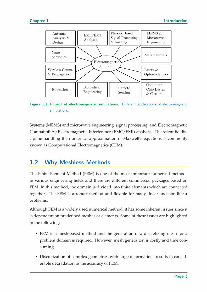
ios are reduced. Electromagnetic simulations have a wide range of applications. Fig-
ure 1.1 shows some applications of electromagnetic simulations including antennas,
nano-photonics, communications, biomedical engineering, remote sensing, chip de-
sign and circuits, lasers and optoelectronics, metamaterials, Micro-Electro-Mechanical
Page 2
Chapter 1 Introduction
Figure 1.1. Impact of electromagnetic simulations. Different applications of electromagnetic
simulations.
Systems (MEMS) and microwave engineering, signal processing, and Electromagnetic
Compatibility/Electromagnetic Interference (EMC/EMI) analysis. The scientific dis-
cipline handling the numerical approximation of Maxwell’s equations is commonly
known as Computational Electromagnetics (CEM).
1.2 Why Meshless Methods
The Finite Element Method (FEM) is one of the most important numerical methods
in various engineering fields and there are different commercial packages based on
FEM. In this method, the domain is divided into finite elements which are connected
together. The FEM is a robust method and flexible for many linear and non-linear
problems.
Although FEM is a widely used numerical method, it has some inherent issues since it
is dependent on predefined meshes or elements. Some of these issues are highlighted
in the following:
• FEM is a mesh-based method and the generation of a discretizing mesh for a
problem domain is required. However, mesh generation is costly and time con-
suming.
• Discretization of complex geometries with large deformations results in consid-
erable degradation in the accuracy of FEM.
Page 3
1.3 Definition of Meshless Methods
• To have an accurate solution for a discretized problem, the quality of the mesh
is very important. An adaptive analysis and re-meshing techniques are required
to obtain a desired accuracy. For re-meshing techniques, the required adaptive
mesh generation leads to additional computational time and cost.
These mentioned problems come from the use of meshes in the FEM. To overcome
these difficulties in the mesh-based numerical methods, meshless methods have been
proposed.
1.3 Definition of Meshless Methods
In meshless methods a set of scattered nodes within the problem domain and on the
boundaries of the domain is used to represent the problem domain. These scattered
nodes are not forming a mesh and so no priori information related to the nodes rela-
tionships is required.
Many meshless methods have found their applications in numerical methods. Al-
though meshless methods have a great potential to become successful and powerful
numerical tools, they are still in the early stage and more developments are required
to solve their technical problems.
1.4 Objectives of the Thesis
The time-domain meshless Radial Point Interpolation Method (RPIM) is investigated
in this thesis. The introductory parts describe general features of meshless methods in
Chapter 2, and more particularly the RPIM framework in Chapter 3. In the first main
part of this thesis in Chapter 4, the focus is on the time-domain staggered meshless
RPIM in three-dimensional (3D) domain. Time-domain meshless methods in electro-
magnetics which are based on solving the first-order Maxwell’s equations have been
proposed in [19, 20, 21, 22]. Using this formulation both electric and magnetic fields are
simultaneously unknown and are solved in a time iteration loop. Because of the type of
intrinsic coupling between electric (E) and magnetic (H) fields expressed in Maxwell’s
curl equations, the magnetic field values are best sampled between the locations where
the electric field values are sampled. Therefore, the computational domain needs to be
discretized by staggered electric and magnetic node distributions. To this end, an ini-
tial node distribution can be generated randomly for the electric field E and then a
Page 4
Chapter 1 Introduction
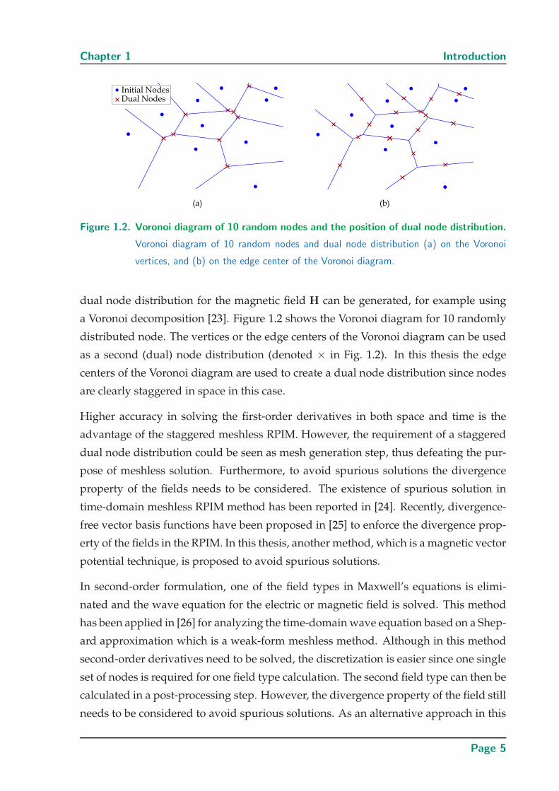
Figure 1.2. Voronoi diagram of 10 random nodes and the position of dual node distribution.
Voronoi diagram of 10 random nodes and dual node distribution (a) on the Voronoi
vertices, and (b) on the edge center of the Voronoi diagram.
dual node distribution for the magnetic field H can be generated, for example using
a Voronoi decomposition [23]. Figure 1.2 shows the Voronoi diagram for 10 randomly
distributed node. The vertices or the edge centers of the Voronoi diagram can be used
as a second (dual) node distribution (denoted × in Fig. 1.2). In this thesis the edge
centers of the Voronoi diagram are used to create a dual node distribution since nodes
are clearly staggered in space in this case.
Higher accuracy in solving the first-order derivatives in both space and time is the
advantage of the staggered meshless RPIM. However, the requirement of a staggered
dual node distribution could be seen as mesh generation step, thus defeating the pur-
pose of meshless solution. Furthermore, to avoid spurious solutions the divergence
property of the fields needs to be considered. The existence of spurious solution in
time-domain meshless RPIM method has been reported in [24]. Recently, divergence-
free vector basis functions have been proposed in [25] to enforce the divergence prop-
erty of the fields in the RPIM. In this thesis, another method, which is a magnetic vector
potential technique, is proposed to avoid spurious solutions.
In second-order formulation, one of the field types in Maxwell’s equations is elimi-
nated and the wave equation for the electric or magnetic field is solved. This method
has been applied in [26] for analyzing the time-domain wave equation based on a Shep-
ard approximation which is a weak-form meshless method. Although in this method
second-order derivatives need to be solved, the discretization is easier since one single
set of nodes is required for one field type calculation. The second field type can then be
calculated in a post-processing step. However, the divergence property of the field still
needs to be considered to avoid spurious solutions. As an alternative approach in this
Page 5
1.5 Statement of Original Contribution
category, the solution of the wave equation for the vector potential can be considered,
as demonstrated for the finite-difference time-domain method in [27]. An adaptation
of this approach for the time-domain meshless RPIM is proposed in the second major
part of the thesis.
In the second main part, Chapters 5 and 6 propose non-staggered meshless RPIM us-
ing the magnetic vector potential technique. The specific implementation is based on
the local calculation of the magnetic vector potential in small support domains. Con-
sidering the relation for the magnetic flux density B = ∇×A and J as a current source,
the magnetic vector potential A satisfies the inhomogeneous wave equation as
∇2A − µǫ∂2A
∂t2= −µJ. (1.2)
Using RPIM to discretize the space derivatives and finite differences to discretize the
time derivatives in (1.2) lead to the discretized expression for the magnetic vector po-
tential. In this formulation the divergence property of the fields is automatically en-
forced, and a single set of nodes is required in the discretized domain for computing
the magnetic vector potential. Boundary conditions for the magnetic vector potential
can be adapted from the boundary conditions for the electric or magnetic fields. How-
ever, applying boundary conditions for the magnetic vector potential is not straight-
forward since they are related to the derivatives of the magnetic vector potential com-
ponents.
1.5 Statement of Original Contribution
This thesis includes several original contributions in meshless RPIM. The original con-
tributions can be described in two major parts. The first main part of the thesis is fo-
cused on the staggered meshless RPIM. The second main part of the thesis investigates
the non-staggered meshless RPIM.
1.5.1 Staggered Meshless RPIM
This section lists the original contributions of the first major part of the thesis, which is
focused on the staggered meshless RPIM.
• The behavior of two different types of basis functions for the meshless RPIM is
investigated. A 2D test function is interpolated through Gaussian and Wendland
Page 6
Chapter 1 Introduction
basis functions and the approximation errors on the low-order derivatives of the
test function are calculated. It is shown that the Gaussian basis function is more
appropriate for the interpolation in small support domains, whereas Wendland
basis function is more accurate for larger support domains. The results were pre-
sented at the International Conference on Computational Electromagnetics (iCCEM),
2015 and is published in the proceedings under the title “On the choice of ba-
sis functions for the meshless radial point interpolation method with small local
support domains” [4].
• The time-domain behavior of the Uniaxial Perfectly Matched Layer (UPML) in
the 3D meshless RPIM is investigated. It is theoretically shown that the UPML
will become unstable after a very long time, when the energy in the computa-
tional domain almost completely vanishes. A timed introduction of loss terms
in the equations inside the UPMLs, i.e. at a time after absorption of most of the
energy, can significantly delay or even remove the occurrence of this instabil-
ity without compromising the accuracy of the solution. The proposed method
was presented at the Asia-Pacific Microwave Conference (APMC), 2013 and is pub-
lished in the proceedings under the title “On the late-time instability of perfectly
matched layers in the meshless radial point interpolation method” [10].
• The effect of different node distributions on the accuracy of electromagnetic sim-
ulations performed with meshless method is investigated. As a test case, a rectan-
gular waveguide truncated with Perfectly Matched Layers (PMLs) is simulated
using the 3D meshless RPIM in the time domain. For the discretization of the
geometry, different strategies of node distribution are utilized, namely, a uniform
grid distribution, a cylindrical node distribution, and disturbed grid distribu-
tions with random displacements amounting to 5% and 10% of the grid average
node distance. All distributions are generated with a similar node density, and
the results are compared in terms of phase and amplitude of the propagating
wave. The application of RPIM in all cases demonstrates similar levels of error,
which indicates the robustness of this meshless algorithm with respect to differ-
ent node distribution strategies. The results of the study were presented at the
Asia-Pacific Microwave Conference (APMC), 2012 and are published in the proceed-
ings under the title “Impact of different node distributions on the meshless radial
point interpolation method in time-domain electromagnetic simulations” [11].
Page 7
1.5 Statement of Original Contribution
• The capability of the meshless RPIM for implementing several arbitrarily ori-
entated regular grids is investigated. For this purpose, a waveguide Y-junction
diplexer is simulated with a 3D RPIM time-domain solver. The result of the
study was published in a book chapter under the title “Conformal and Multi-
Scale Time-Domain Methods: From Unstructured Meshes to Meshless Discretiza-
tions”, published by Springer-Verlag [1].
• The scattering from a perfect electrically conducting sphere is implemented using
3D meshless RPIM and the simulated far-field patterns are compared with the
theoretical results. To this end, the perfect electric sphere is simulated in a 3D
domain, which is truncated by the PMLs. To compute the far-field pattern, first
the simulated electric and magnetic current densities are obtained on a so-called
Huygens’ surface. Then using a near-field to far-field transformation, far-field
scattering from a conductive sphere is obtained and compared to the theoretical
Mie solution. It is shown that simulation and theoretical results are in a good
agreement.
1.5.2 Non-Staggered Meshless RPIM
This section lists the original contributions of the second major part of the thesis, which
is focused on the non-staggered meshless RPIM.
• A time-domain vector potential solver for the analysis of transient electromag-
netic field with the meshless RPIM is proposed. Solving the second-order vector
potential wave equation enforces the divergence-free property of the fields and
avoids computational effort related to a dual node distribution required for solv-
ing the first-order Maxwell equations. The proposed method is validated with
several examples of 2D parallel plate waveguide and filters, and the convergence
is empirically demonstrated in terms of node density or size of local support
domains. It is further shown that inhomogeneous node distributions can pro-
vide accelerated convergence, i.e., the same accuracy with smaller number of
nodes compared to a solution for homogeneous node distribution. The proposed
method is published in International Journal for Numerical methods in Engineering
(IJNME) under the title “Time-domain vector potential technique for the mesh-
less radial point interpolation method” [2].
Page 8
Chapter 1 Introduction
• A hybrid algorithm for the implementation of PMLs in the meshless magnetic
vector potential technique is proposed. Solving the wave equation in time-domain,
the magnetic vector potential technique avoids using staggered node distribu-
tions which are needed for calculating the E and H fields when directly solving
Maxwell’s equations. However, implementing PMLs with stretched coordinate
formulation requires auxiliary variables on a staggered (dual) node distribution.
To avoid defining staggered nodes in the whole computational domain, a hybrid
algorithm is proposed: The algorithm keeps a single set of nodes for the mag-
netic vector potential A inside the free space, while it uses staggered nodes for
A and auxiliary variables inside the PML. The hybrid algorithm is validated in a
2D rectangular waveguide and numerical reflection coefficients are compared for
different thicknesses of the PML and for different orders of a polynomial conduc-
tivity profile inside the PML. A good agreement between theoretical results and
converged solutions validates the approach, with best performance using a poly-
nomial order m = 3. The proposed method was presented at the International
Workshop on Antenna Technology (iWAT), 2014 and is published in the proceed-
ings under the title “Hybrid staggered perfectly matched layers in non-staggered
meshless time-domain vector potential technique” [6]. This paper was awarded
the best student paper award of iWAT 2014.
• Two different approaches for the time-domain meshless RPIM in electromagnetic
simulations are compared. These two algorithms are categorized based on the or-
der of partial differential equations which are needed for solving electromagnetic
problems. Then the advantages and issues related to those two types of formu-
lations are discussed. The results were presented at the 1st Australian Microwave
Symposium (AMS), 2014 and is published in the proceedings under the title “First-
and second-order meshless radial point interpolation methods in electromagnet-
ics” [7]. This paper was awarded the best student paper award of AMS 2014.
• The performance of the staggered and non-staggered RPIM for time-domain elec-
tromagnetics are compared. As an illustrative example, the scattering parame-
ters of a waveguide filter are computed using both staggered and non-staggered
RPIM. The accuracy of the results obtained with both methods is assessed through
comparison with a reference solution. The results were presented at the 17th In-
ternational Symposium on ElectroMagnetic Compatibility (CEM), 2014 and is pub-
lished in the proceedings under the title “On the staggered and non-staggered
Page 9
1.6 Overview of the Thesis
time-domain meshless radial point interpolation method” [8]. This paper was
awarded the best conference paper award of CEM 2014.
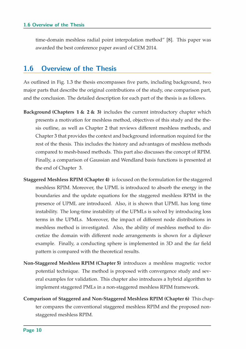
1.6 Overview of the Thesis
As outlined in Fig. 1.3 the thesis encompasses five parts, including background, two
major parts that describe the original contributions of the study, one comparison part,
and the conclusion. The detailed description for each part of the thesis is as follows.
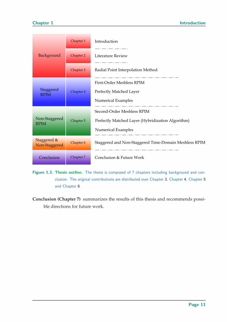
Background (Chapters 1 & 2 & 3) includes the current introductory chapter which
presents a motivation for meshless method, objectives of this study and the the-
sis outline, as well as Chapter 2 that reviews different meshless methods, and
Chapter 3 that provides the context and background information required for the
rest of the thesis. This includes the history and advantages of meshless methods
compared to mesh-based methods. This part also discusses the concept of RPIM.
Finally, a comparison of Gaussian and Wendland basis functions is presented at
the end of Chapter 3.
Staggered Meshless RPIM (Chapter 4) is focused on the formulation for the staggered
meshless RPIM. Moreover, the UPML is introduced to absorb the energy in the
boundaries and the update equations for the staggered meshless RPIM in the
presence of UPML are introduced. Also, it is shown that UPML has long time
instability. The long-time instability of the UPMLs is solved by introducing loss
terms in the UPMLs. Moreover, the impact of different node distributions in
meshless method is investigated. Also, the ability of meshless method to dis-
cretize the domain with different node arrangements is shown for a diplexer
example. Finally, a conducting sphere is implemented in 3D and the far field
pattern is compared with the theoretical results.
Non-Staggered Meshless RPIM (Chapter 5) introduces a meshless magnetic vector
potential technique. The method is proposed with convergence study and sev-
eral examples for validation. This chapter also introduces a hybrid algorithm to
implement staggered PMLs in a non-staggered meshless RPIM framework.
Comparison of Staggered and Non-Staggered Meshless RPIM (Chapter 6) This chap-
ter compares the conventional staggered meshless RPIM and the proposed non-
staggered meshless RPIM.
Page 10
Chapter 1 Introduction
Figure 1.3. Thesis outline. The thesis is composed of 7 chapters including background and con-
clusion. The original contributions are distributed over Chapter 3, Chapter 4, Chapter 5
and Chapter 6.
Conclusion (Chapter 7) summarizes the results of this thesis and recommends possi-
ble directions for future work.
Page 11

Page 12
Chapter 2
Overview of Mesh-basedand Meshless Methods
THE different numerical methods for the solution of partial dif-
ferential equations can be classified into two categories: mesh-
based and meshless methods. This chapter reviews these two cat-
egories for the numerical solution of Maxwell’s equations. In mesh-based
methods two representative methods, namely, the Finite-Difference Time-
Domain (FDTD) method and the Finite Element Method (FEM), are intro-
duced briefly. In meshless methods a historical overview of the approach
is first presented. Then the solution procedure in meshless methods is de-
scribed. Moreover, different meshless methods are introduced and classi-
fied in terms of formulation and approximation schemes. Finally, variations
of meshless methods with different shape functions are introduced.
Page 13
2.1 Introduction
2.1 Introduction
There are many different numerical methods in electromagnetics. These techniques
can be classified by whether they are based on integral or differential equations, whether
they operate in the time or frequency domain, and whether they are mesh-based or
meshless methods. This chapter describes mesh-based and meshless methods.
In the first part of this chapter mesh-based methods are reviewed. In the mesh-based
category, the Finite-Difference Time-Domain (FDTD) method and the Finite Element
Method (FEM) are explained and their applications in electromagnetics are provided.
Then in the second part, after a brief introduction to meshless methods, main steps
in meshless methods are explained. Also, different meshless methods are classified in
two different ways and finally some meshless methods with various shape functions
are introduced.
2.2 Mesh-based Methods
In mesh-based methods, the computational domain is discretized in a partition of nu-
merous finite volumes, elements, or cells. Note that the mesh discretization needs to
be generated in a pre-processing step or dynamically modified in adaptive meshing
methods as the solution progresses. Maxwell’s equations are then approximated on
the elements of the structure and a system of equations is obtained. In order to find
the unknown solution, the system of equations is solved using appropriate numeri-
cal methods. Some important numerical mesh-based methods are: FDTD, Method of
Moment (MoM), and FEM.
In 1966, Yee introduced the FDTD method in electromagnetic modeling [28]. He pro-
posed a special algorithm for discretizing the space of electromagnetic problems. Since
then many other finite-difference algorithms have been introduced to discretize Max-
well’s equations, but none of them have been as robust as Yee’s method [29]. This
method being implemented in the time domain, the responses in a chosen frequency
range can be computed in a single simulation run. Also, non-linear responses can be
naturally calculated by this type of methods [29].
The MoM in electromagnetics was introduced as one of the first numerical methods
for the analysis of antennas and scatterers. This method discretizes the integral equa-
tions. It is generally based on surfaces and currents, whereas FEM and FDTD are
Page 14
Chapter 2 Overview of Mesh-based and Meshless Methods
based on volumes and fields. This means that in the classical form of MoM, only the
material interfaces are discretized and solved, whereas for FEM and FDTD all volumes
of interest must be discretized [30]. The general idea of MoM was introduced by Boris
Grigoryevich Galerkin before 1920. In electromagnetics, MoM was first utilized by No-
mura in 1952 [31] and Storm in 1953 [32] for linear antennas. Later, the mathematical
foundations of the MoM were introduced in 1964 by Kantorovich, et al. [33, 34]. The
MoM became popular following the work of Harrington, who proposed a systematic
approach for the method in 1967-1968 [35, 36].
FEM is a more powerful method than FDTD and MoM for complex geometries and
inhomogeneous media [18]. Although FEM was introduced by Courant in 1943 [37],
it has not been widely used in electronic engineering until 1969, when FEM found its
application in electromagnetics [38, 39]. Today, FEM is widely adopted and powerful
commercial FEM software tools are available.
In this section, the FDTD method and the FEM are reviewed since some of their con-
cepts are used in the meshless methods as well.
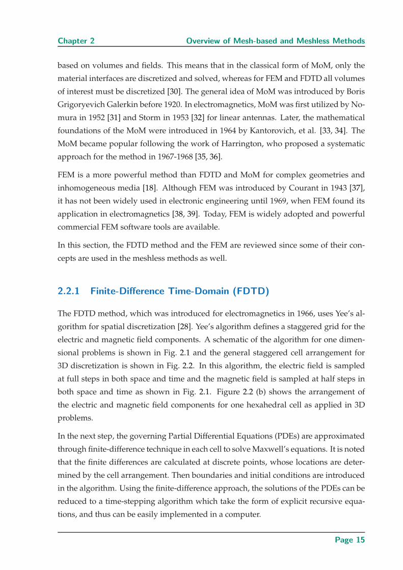
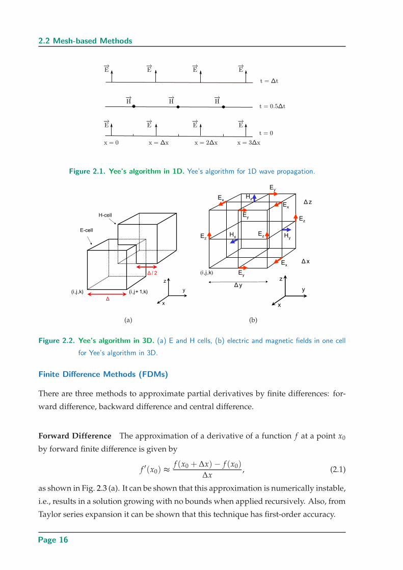
2.2.1 Finite-Difference Time-Domain (FDTD)
The FDTD method, which was introduced for electromagnetics in 1966, uses Yee’s al-
gorithm for spatial discretization [28]. Yee’s algorithm defines a staggered grid for the
electric and magnetic field components. A schematic of the algorithm for one dimen-
sional problems is shown in Fig. 2.1 and the general staggered cell arrangement for
3D discretization is shown in Fig. 2.2. In this algorithm, the electric field is sampled
at full steps in both space and time and the magnetic field is sampled at half steps in
both space and time as shown in Fig. 2.1. Figure 2.2 (b) shows the arrangement of
the electric and magnetic field components for one hexahedral cell as applied in 3D
problems.
In the next step, the governing Partial Differential Equations (PDEs) are approximated
through finite-difference technique in each cell to solve Maxwell’s equations. It is noted
that the finite differences are calculated at discrete points, whose locations are deter-
mined by the cell arrangement. Then boundaries and initial conditions are introduced
in the algorithm. Using the finite-difference approach, the solutions of the PDEs can be
reduced to a time-stepping algorithm which take the form of explicit recursive equa-
tions, and thus can be easily implemented in a computer.
Page 15
2.2 Mesh-based Methods
1D
−→E
−→E
−→E
−→E
−→E
−→E
−→E
−→E
−→H
−→H
−→H
x = 0 x = ∆x x = 2∆x x = 3∆x
t = 0
t = 0.5∆t
t = ∆t
Figure 2.1. Yee’s algorithm in 1D. Yee’s algorithm for 1D wave propagation.
(a) (b)
Figure 2.2. Yee’s algorithm in 3D. (a) E and H cells, (b) electric and magnetic fields in one cell
for Yee’s algorithm in 3D.
Finite Difference Methods (FDMs)
There are three methods to approximate partial derivatives by finite differences: for-
ward difference, backward difference and central difference.
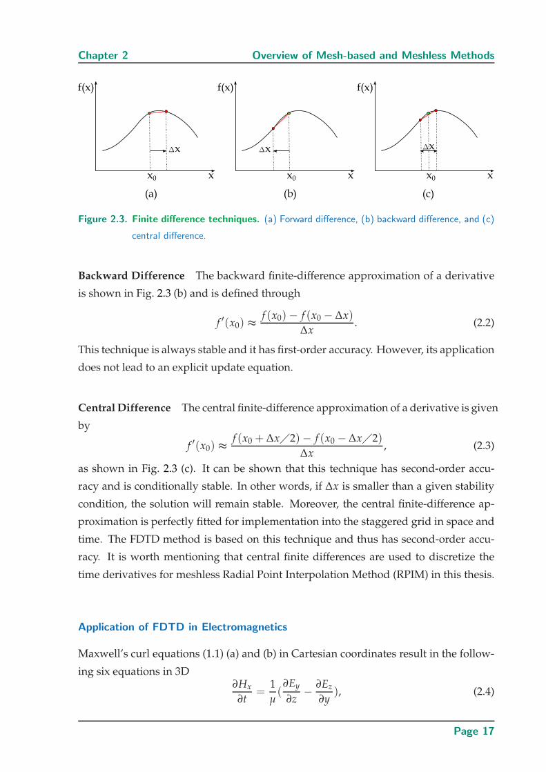
Forward Difference The approximation of a derivative of a function f at a point x0
by forward finite difference is given by
f ′(x0) ≈f (x0 + ∆x)− f (x0)
∆x, (2.1)
as shown in Fig. 2.3 (a). It can be shown that this approximation is numerically instable,
i.e., results in a solution growing with no bounds when applied recursively. Also, from
Taylor series expansion it can be shown that this technique has first-order accuracy.
Page 16
Chapter 2 Overview of Mesh-based and Meshless Methods
Figure 2.3. Finite difference techniques. (a) Forward difference, (b) backward difference, and (c)
central difference.
Backward Difference The backward finite-difference approximation of a derivative
is shown in Fig. 2.3 (b) and is defined through
f ′(x0) ≈f (x0)− f (x0 − ∆x)
∆x. (2.2)
This technique is always stable and it has first-order accuracy. However, its application
does not lead to an explicit update equation.
Central Difference The central finite-difference approximation of a derivative is given
by
f ′(x0) ≈f (x0 + ∆x2)− f (x0 − ∆x2)
∆x, (2.3)
as shown in Fig. 2.3 (c). It can be shown that this technique has second-order accu-
racy and is conditionally stable. In other words, if ∆x is smaller than a given stability
condition, the solution will remain stable. Moreover, the central finite-difference ap-
proximation is perfectly fitted for implementation into the staggered grid in space and
time. The FDTD method is based on this technique and thus has second-order accu-
racy. It is worth mentioning that central finite differences are used to discretize the
time derivatives for meshless Radial Point Interpolation Method (RPIM) in this thesis.
Application of FDTD in Electromagnetics
Maxwell’s curl equations (1.1) (a) and (b) in Cartesian coordinates result in the follow-
ing six equations in 3D∂Hx
∂t=
1
µ(
∂Ey
∂z− ∂Ez
∂y), (2.4)
Page 17
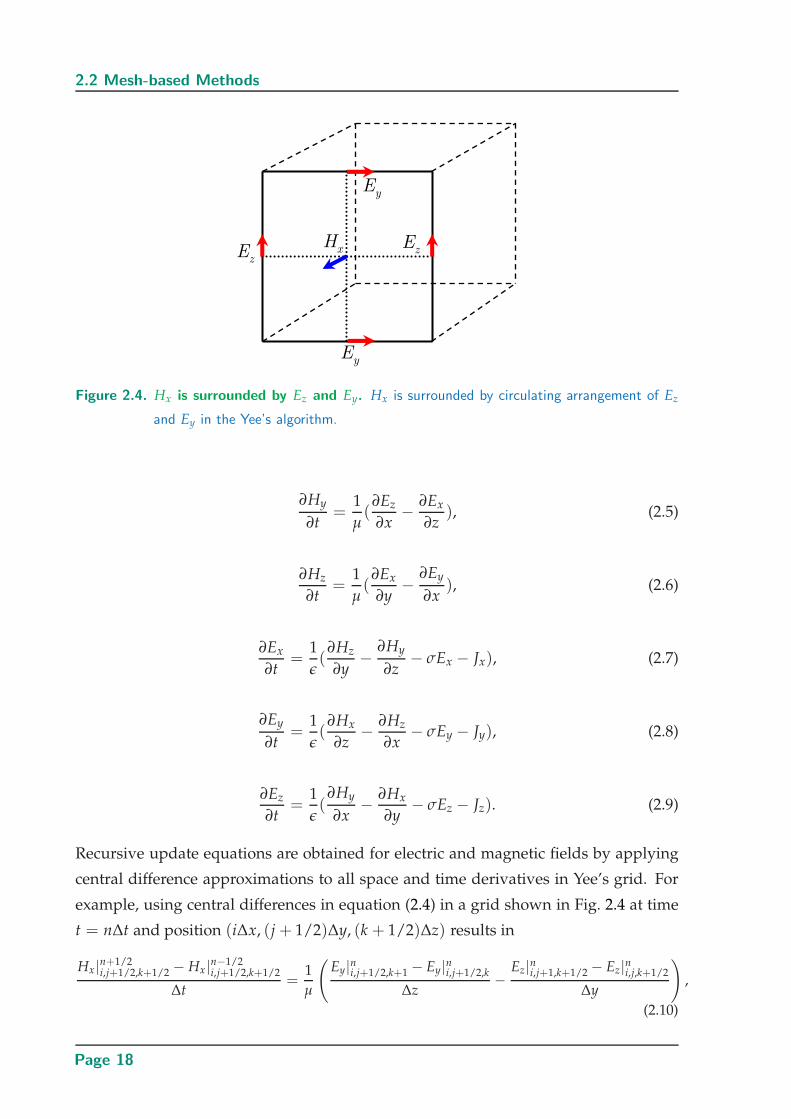
2.2 Mesh-based Methods
Hx
Ey
Ey
EzE
z
Figure 2.4. Hx is surrounded by Ez and Ey. Hx is surrounded by circulating arrangement of Ez
and Ey in the Yee’s algorithm.
∂Hy
∂t=
1
µ(
∂Ez
∂x− ∂Ex
∂z), (2.5)
∂Hz
∂t=
1
µ(
∂Ex
∂y− ∂Ey
∂x), (2.6)
∂Ex
∂t=
1
ǫ(
∂Hz
∂y− ∂Hy
∂z− σEx − Jx), (2.7)
∂Ey
∂t=
1
ǫ(
∂Hx
∂z− ∂Hz
∂x− σEy − Jy), (2.8)
∂Ez
∂t=
1
ǫ(
∂Hy
∂x− ∂Hx
∂y− σEz − Jz). (2.9)
Recursive update equations are obtained for electric and magnetic fields by applying
central difference approximations to all space and time derivatives in Yee’s grid. For
example, using central differences in equation (2.4) in a grid shown in Fig. 2.4 at time
t = n∆t and position (i∆x, (j + 1/2)∆y, (k + 1/2)∆z) results in
Hx|n+1/2i,j+1/2,k+1/2 − Hx|n−1/2
i,j+1/2,k+1/2
∆t=
1
µ
(Ey|ni,j+1/2,k+1 − Ey|ni,j+1/2,k
∆z−
Ez|ni,j+1,k+1/2 − Ez|ni,j,k+1/2
∆y
),
(2.10)
Page 18
Chapter 2 Overview of Mesh-based and Meshless Methods
Hz
Ex
Hy
Hy
Hz
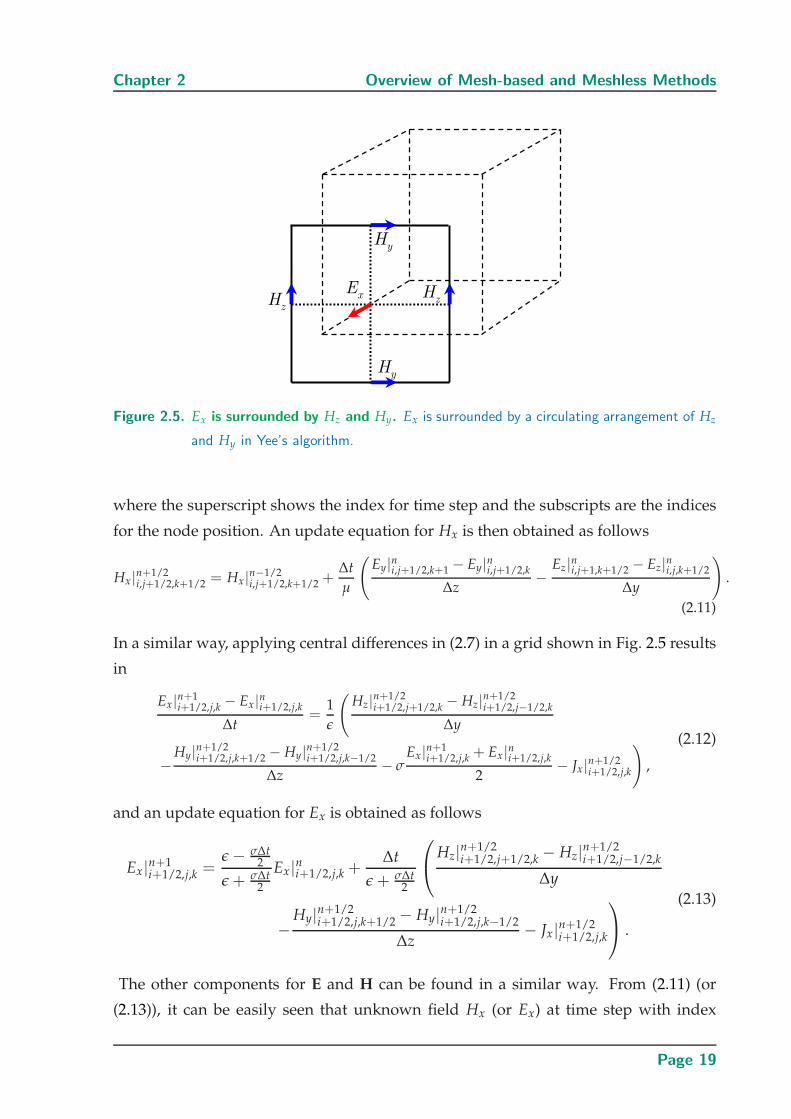
Figure 2.5. Ex is surrounded by Hz and Hy. Ex is surrounded by a circulating arrangement of Hz
and Hy in Yee’s algorithm.
where the superscript shows the index for time step and the subscripts are the indices
for the node position. An update equation for Hx is then obtained as follows
Hx|n+1/2i,j+1/2,k+1/2 = Hx|n−1/2
i,j+1/2,k+1/2 +∆t
µ
(Ey|ni,j+1/2,k+1 − Ey|ni,j+1/2,k
∆z−
Ez|ni,j+1,k+1/2 − Ez|ni,j,k+1/2
∆y
).
(2.11)
In a similar way, applying central differences in (2.7) in a grid shown in Fig. 2.5 results
in
Ex|n+1i+1/2,j,k − Ex|ni+1/2,j,k
∆t=
1
ǫ
(Hz|n+1/2
i+1/2,j+1/2,k − Hz|n+1/2i+1/2,j−1/2,k
∆y
−Hy|n+1/2
i+1/2,j,k+1/2 − Hy|n+1/2i+1/2,j,k−1/2
∆z− σ
Ex|n+1i+1/2,j,k + Ex|ni+1/2,j,k
2− Jx|n+1/2
i+1/2,j,k
),
(2.12)
and an update equation for Ex is obtained as follows
Ex|n+1i+1/2,j,k =
ǫ − σ∆t2
ǫ + σ∆t2
Ex|ni+1/2,j,k +∆t
ǫ + σ∆t2
Hz|n+1/2i+1/2,j+1/2,k − Hz|n+1/2
i+1/2,j−1/2,k
∆y
−Hy|n+1/2
i+1/2,j,k+1/2 − Hy|n+1/2i+1/2,j,k−1/2
∆z− Jx|n+1/2
i+1/2,j,k
.
(2.13)
The other components for E and H can be found in a similar way. From (2.11) (or
(2.13)), it can be easily seen that unknown field Hx (or Ex) at time step with index
Page 19
2.2 Mesh-based Methods
n + 1/2 (or n + 1) can be found from known field values at previous time steps, with
indices n − 1/2 and n (or n and n + 1/2). Initial values or time-dependent sources are
applied to the equations before the start of the iteration.
To achieve good accuracy in simulations, the spatial discretization needs to be cho-
sen smaller than the simulated wavelength. Although decreasing the discretization
steps decreases the error, it also decreases the required time step (as mentioned in next
paragraph), which slows the time iteration. A good trade off between accuracy and
efficiency is a discretization between λ/10 and λ/20.
To have a stable simulation, the time step ∆t has to be bounded by a value which is
determined by the space discretization. In 3D simulation, the stability condition for
the time step ∆t is determined by
∆t ≤ 1
c ·√
1(∆x)2 +
1(∆y)2 +
1(∆z)2
, (2.14)
where c is the speed of light in free space, ∆x, ∆y and ∆z are the spatial steps in x, y
and z-directions. This condition is called the Courant-Friedrich-Levy condition [29].
2.2.2 Finite Element Method (FEM)
The FEM found its first application in electromagnetics in 1969 [38], [39]. Basic steps in
FEM are as follows [40, 41]
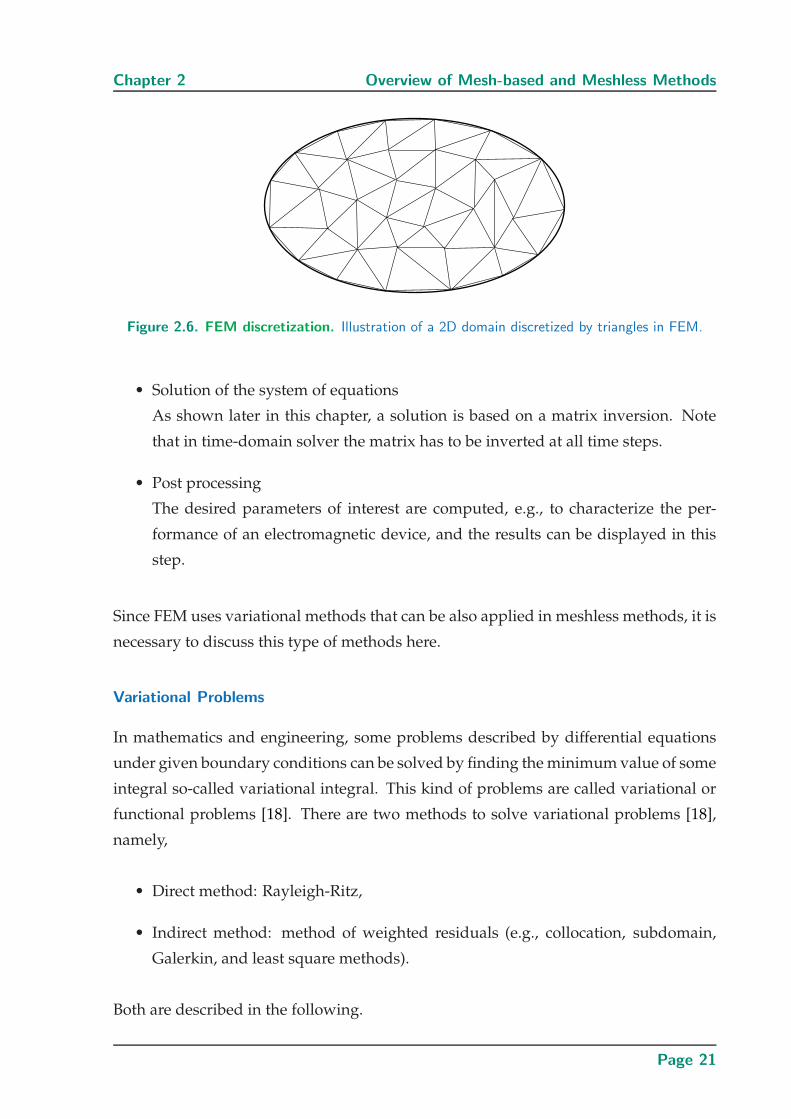
• Domain discretization
The whole geometry of interest is divided into a partition of elements, which are
usually triangles in 2D and tetrahedrons in 3D as shown in Fig. 2.6.
• Selection of interpolation functions
Interpolation functions provide an approximate solution within an element. They
are usually polynomial functions. High-order polynomials are very accurate but
their formulations are more complex than low-order polynomials.
• Formulation of equations
The Rayligh-Ritz and Galerkin methods can be used to formulate the system of
equations. The problem is first formulated in each element. Then, interaction
with other elements are considered and a global matrix for the system of equa-
tions is found.
Page 20
Chapter 2 Overview of Mesh-based and Meshless Methods
Figure 2.6. FEM discretization. Illustration of a 2D domain discretized by triangles in FEM.
• Solution of the system of equations
As shown later in this chapter, a solution is based on a matrix inversion. Note
that in time-domain solver the matrix has to be inverted at all time steps.
• Post processing
The desired parameters of interest are computed, e.g., to characterize the per-
formance of an electromagnetic device, and the results can be displayed in this
step.
Since FEM uses variational methods that can be also applied in meshless methods, it is
necessary to discuss this type of methods here.
Variational Problems
In mathematics and engineering, some problems described by differential equations
under given boundary conditions can be solved by finding the minimum value of some
integral so-called variational integral. This kind of problems are called variational or
functional problems [18]. There are two methods to solve variational problems [18],
namely,
• Direct method: Rayleigh-Ritz,
• Indirect method: method of weighted residuals (e.g., collocation, subdomain,
Galerkin, and least square methods).
Both are described in the following.
Page 21
2.2 Mesh-based Methods
Rayleigh-Ritz Method In the Rayleigh-Ritz method, an approximate solution with
unknown coefficients is substituted into the relevant functional equation. This approx-
imate solution is assumed to be a linearly independent set of functions, which is de-
fined over the domain and satisfies the boundary conditions. Unknown coefficients in
the approximate solution are determined by minimizing the functional equation with
respect to those coefficients. Consequently an approximated solution will be deter-
mined. The Rayleigh-Ritz method has two major limitations. These limitations are
• There is no variational equivalent for some problems,
• It is difficult to apply boundary conditions to an approximate solution in some
complex geometries.
Therefore, if a suitable functional does not exist for the above method, the weighted
residual method will be more appropriate.
Weighted Residual Method The weighted residual method is more general, and it
is not limited to variational problems. In this method, the residual, i.e., the error due
to the approximate solution, is calculated. Then a weighting function is chosen such
that the inner product of the residual and the weighting function is minimized. In
discrete form, these equations can be converted to a matrix form. Finally, the unknown
coefficients can be calculated from the obtained matrix equation.
To understand how to use the residual of the differential equation to solve the problem,
we assume that we start from the equation
L(u) = g, (2.15)
with a linear operator L. In this equation u is the unknown quantity and g is the exci-
tation (source). The solution of this equation inside each element can be approximated
by the following finite series
u ≈ uh =N
∑n=1
an fn, (2.16)
Where an are coefficients, uh is the approximated value for u, and fn are referred as
basis or shape functions. The scalar basis function fn is assumed to have a unitary
value at node n and zero at other nodes. Accuracy and efficiency of the weighting
method is dependent on the selection of the basis functions. Basis functions should
satisfy the two conditions below
Page 22
Chapter 2 Overview of Mesh-based and Meshless Methods
• Basis functions should satisfy the boundary conditions for the linear operator (L),
• Basis functions must results in a complete set to accurately describe the field [18].
The residual R (amount of error due to this approximation) is given by
R = g −N
∑n=1
anL( fn). (2.17)
To find the best approximation for uh, the residual function should be minimized at
all points in the domain through the weighting function W. In other words, the inner
product of R and W should be zero. An inner product of functions u and v defined on
domain Ω is denoted here as 〈u, v〉 and can be written as
〈u, v〉 =∫
Ωuv∗dΩ, (2.18)
where ∗ shows the complex conjugate. Therefore, we have
〈R, W〉 = 0. (2.19)
The weighting function W is usually written as finite series
W =M
∑m=1
Wm. (2.20)
Substituting (2.17) in (2.19) gives M equations of the form
N
∑n=1
an〈Wm, L( fn)〉 = 〈Wm, g〉. (2.21)
Equation 2.21 can be rewritten in a matrix form as follows
ZI = V, (2.22)
where the matrix elements are as follows
Zmn = 〈Wm, L( fn)〉, (2.23a)
In = an, (2.23b)
Vm = 〈Wm, g〉. (2.23c)
Unknown coefficients I in (2.22) can be found as
I = Z−1V. (2.24)
Page 23
2.2 Mesh-based Methods
1
2 3
P
edge1
edge2
edge3
Figure 2.7. A triangle in FEM. A triangle in FEM.
Finally, by substituting the unknown coefficients (2.24) (IT = [a1, a2, · · · , aN ]) in equa-
tion 2.16, an approximated solution will be obtained.
There are different ways to choose weighting functions which lead to: point collocation
method, subdomain collocation method, Galerkin’s method, and least squares method
[18]. As a widespread implementation, in the Galerkin’s method, the weighting func-
tions Wm are same as basis functions fn.
Vector Elements in FEM
Scalar basis functions fn (nodal elements) can be used to find scalar functions and
they are not suitable for finding vector functions. Using nodal elements to represent
vector fields causes some problems such as the inconvenience of imposing boundary
conditions and the occurrence of non-physical or spurious solutions [41]. Therefore,
edge or vector elements, which are related to the edges of the cells rather than to
their corner nodes, were proposed for solution involving vector fields. With edge el-
ements, applying boundary conditions is much easier for vector fields, and by select-
ing divergence-free vector elements, nonphysical solutions are canceled automatically.
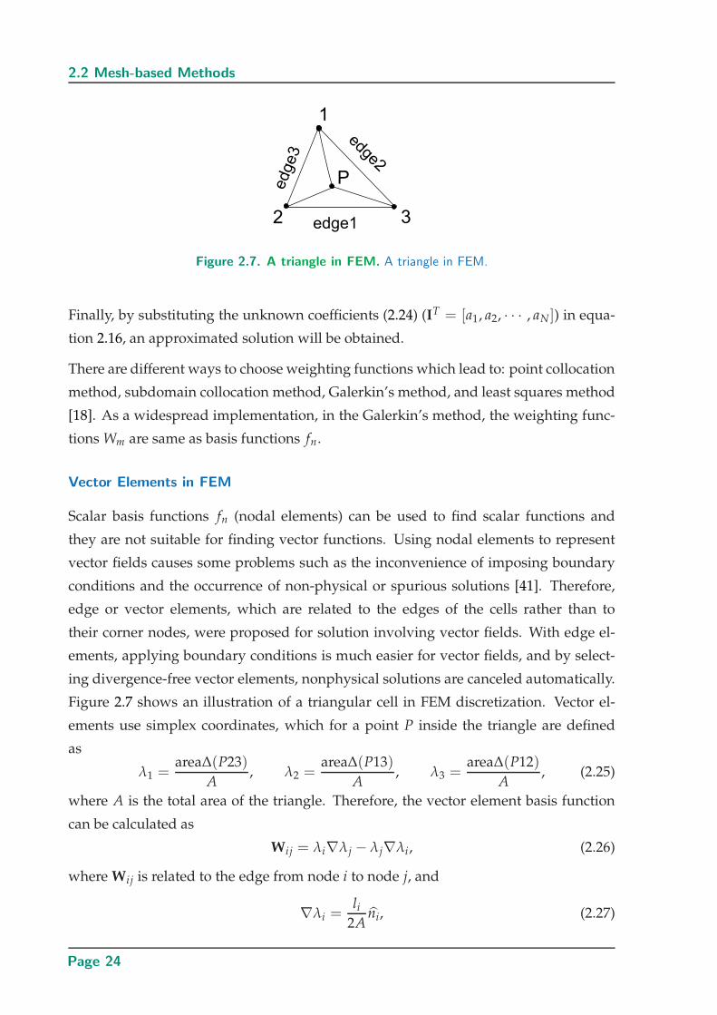
Figure 2.7 shows an illustration of a triangular cell in FEM discretization. Vector el-
ements use simplex coordinates, which for a point P inside the triangle are defined
as
λ1 =area∆(P23)
A, λ2 =
area∆(P13)
A, λ3 =
area∆(P12)
A, (2.25)
where A is the total area of the triangle. Therefore, the vector element basis function
can be calculated as
Wij = λi∇λj − λj∇λi, (2.26)
where Wij is related to the edge from node i to node j, and
∇λi =li
2Ani, (2.27)
Page 24
Chapter 2 Overview of Mesh-based and Meshless Methods
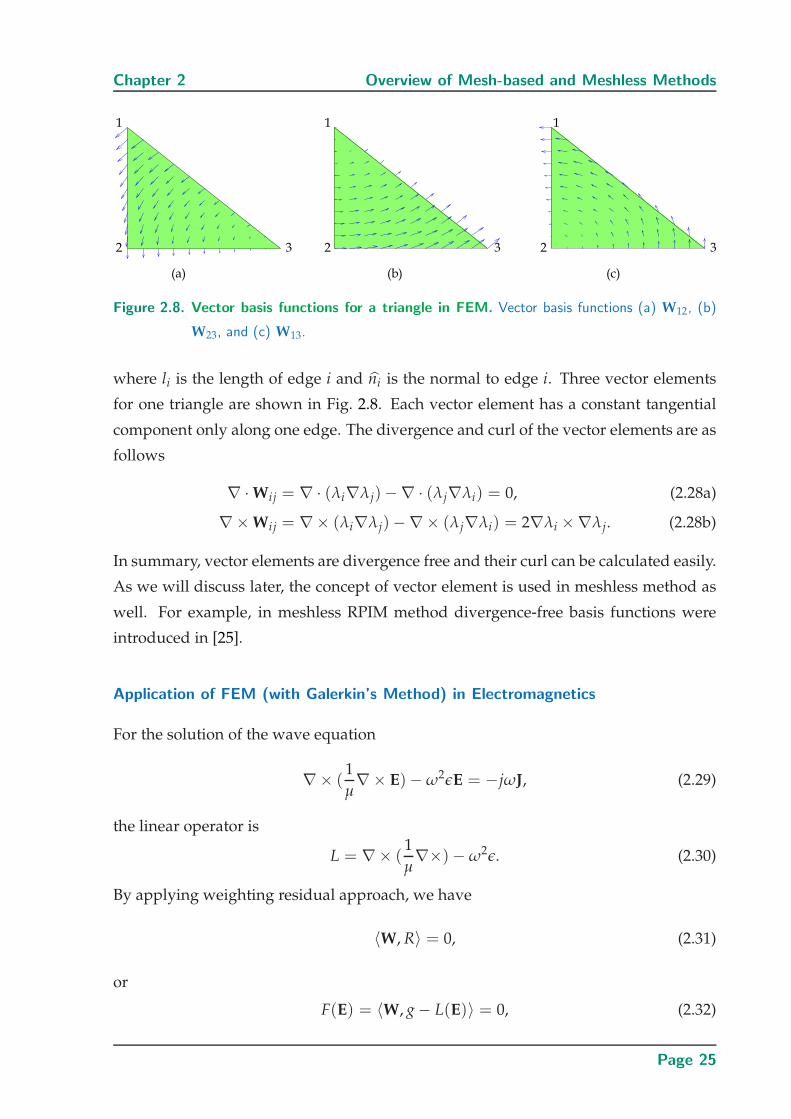
Figure 2.8. Vector basis functions for a triangle in FEM. Vector basis functions (a) W12, (b)
W23, and (c) W13.
where li is the length of edge i and ni is the normal to edge i. Three vector elements
for one triangle are shown in Fig. 2.8. Each vector element has a constant tangential
component only along one edge. The divergence and curl of the vector elements are as
follows
∇ · Wij = ∇ · (λi∇λj)−∇ · (λj∇λi) = 0, (2.28a)
∇× Wij = ∇× (λi∇λj)−∇× (λj∇λi) = 2∇λi ×∇λj. (2.28b)
In summary, vector elements are divergence free and their curl can be calculated easily.
As we will discuss later, the concept of vector element is used in meshless method as
well. For example, in meshless RPIM method divergence-free basis functions were
introduced in [25].
Application of FEM (with Galerkin’s Method) in Electromagnetics
For the solution of the wave equation
∇× (1
µ∇× E)− ω2ǫE = −jωJ, (2.29)
the linear operator is
L = ∇× (1
µ∇×)− ω2ǫ. (2.30)
By applying weighting residual approach, we have
〈W, R〉 = 0, (2.31)
or
F(E) = 〈W, g − L(E)〉 = 0, (2.32)
Page 25
2.2 Mesh-based Methods
where g = −jωJ. We assume that E is approximated by
E =N
∑i=1
ei φi, (2.33)
with basis functions φi, and coefficients ei, which are determined numerically. Substi-
tuting (2.30) in (2.32) gives
F(E) =y
Ω
W ·(∇× (
1
µ∇× E)− ω2ǫE
)dΩ + jω
y
Ω
W · J dΩ, (2.34)
and after some algebraic simplifications the following equation is obtained
F(E) =y
Ω
(∇× W · ∇ × E
µ− ω2ǫW · E
)dΩ − 1
µ
∂Ω
(W ×∇× E) · n dS
+ jωy
Ω
W · J dΩ.(2.35)
Since weighting function and basis functions are identical in Galerkin’s method the
electric field E can be written as
E =N
∑i=1
ei Wi. (2.36)
The matrix form of (2.35) with k0 = ω√
ǫ is as follows
Ae − k20Be + Ce = fe, (2.37)
where
e = (ei), (2.38)
Aij =1
µ
y
Ω
∇× Wi · ∇ × Wj dΩ, (2.39)
Bij =y
Ω
Wi · Wj dΩ, (2.40)
Cij =1
µ
∂Ω
Wi ×∇× Wj dS, (2.41)
fe = jωy
Ω
W · J dΩ. (2.42)
Unknown coefficients ei can be calculated from equation 2.37, and consequently the
solution for the electric field will be found from equation 2.36.
Page 26
Chapter 2 Overview of Mesh-based and Meshless Methods
2.2.3 Limitations of Mesh-based Methods
In spite of their many advantages, mesh-based methods have some issues. They often
do not have enough flexibility for complex geometries, need large computer resources
due to the mesh generation, and might only reach a low-accuracy solution in some
problems. For example, FDTD cannot effectively and accurately simulate problems
that have features at multiple scales, such as resolving small details in an electrically
large structure. Moreover, the accuracy of mesh-based methods depends on the type
and quality of the mesh that is used to discretize the computational domain. Moreover,
it is difficult to generate and modify the mesh since the mesh cells are not independent
and they have an interconnected structure. It is worth mentioning that some mesh-
based methods have been improved to locally increase the accuracy. For example, in
[42], a FDTD variation denoted as “zoom” FDTD has been introduced to discretize the
geometry with different discretizations, e.g., a fine discretization for small dimensions
and a coarse discretization for the rest of the domain. The Equivalent Circuit (EC)
FDTD has also been used in [43] to discretize the geometry of interest by non-uniform
meshes. However, the last mentioned issue of mesh-based methods, which is mesh
generation and interconnection between meshes, is still remaining.
In order to bypass the mesh generation operation which is a complex and time consum-
ing process, meshless methods were proposed recently as an alternative to mesh-based
methods.
2.3 Meshless Methods
Meshless methods have received considerable attention in different fields of study in-
cluding solid mechanics, fluid dynamics, and electromagnetics. A major advantage of
meshless methods is that they rely on node distributions rather than an explicitly de-
fined mesh. Therefore, some difficulties associated with mesh generation can be elimi-
nated. In fact, because of the unstructured nature of the meshless methods, a compari-
son with a structured mesh-based method would be heavily problem-dependent. For
example, for a well-behaved problem, FDTD will be the most efficient approach. How-
ever, complex multi-scale geometries can be discretized by meshless methods more ef-
ficiently, e.g., using locally higher node densities. Moreover, since meshless methods
are based on arbitrary node distributions and each node can be defined independently,
a costly and time-consuming re-meshing process can be replaced by a local adaptive
Page 27
2.3 Meshless Methods
node refinement [44]. In contrast, in mesh-based methods a re-meshing process is nec-
essary for moving material discontinuity or refining meshes.
However, meshless methods in science and engineering especially in electromagnetics
are in their early stages. Therefore, they still require more developments to find their
places among more established and robust techniques based on Finite Difference (FD),
Finite Element (FE), and Finite Volume (FV) algorithms. Meshless methods are also
called meshfree, gridless, element-free, or cloud methods in the literature [45].
2.3.1 Historical Overview
The idea of mesh-free method comes from Gingold [46] and Lucy [47] in 1977. They
introduced a Lagrangian method based on the kernel estimates method to model as-
trophysics problems such as exploding stars. This method, called Smoothed Particle
Hydrodynamics (SPH) [48, 49, 50], was later widely extended in particular for contin-
uum solid and fluid mechanics. A decade after the introduction of the SPH method, the
mesh-free method was introduced by Nayroles and Touzot in 1992 [51]. Their method,
which is based on Galerkin’s technique, is called Diffuse Element Method (DEM). In
the DEM algorithm, the FEM interpolation was replaced within an element by the
Moving Least Square (MLS) local interpolation [52]. In 1993, the DEM was applied
to model two-dimensional static problems by Yves Marechal [53]. Since then differ-
ent meshless methods have been developed with many different names, including the
wavelet Galerkin method [54], Element-Free Galerkin (EFG) [55, 56, 45], particle-in-cell
method [57], Reproducing Kernel Particle Method (RKPM) [58, 59], Partition of Unity
(PU) [60, 61], hp clouds [62, 63], Finite Point Method (FPM) [64, 65], free-mesh method
[66], meshless local boundary integration equation method, Meshless Local Petrov-
Galerkin method (MLPG) [67, 68], and multi-scale methods [69, 70, 71, 72]. These dif-
ferent meshless methods will be briefly introduced and classified later in this chapter.
2.3.2 Main Steps in Meshless Methods
The main steps to find the solution in meshless methods are as follows
• Domain representation and node generation
In this step, the computational domain and its boundary are discretized by a set
of scattered nodes. The density of nodes depends on the desired accuracy.
Page 28
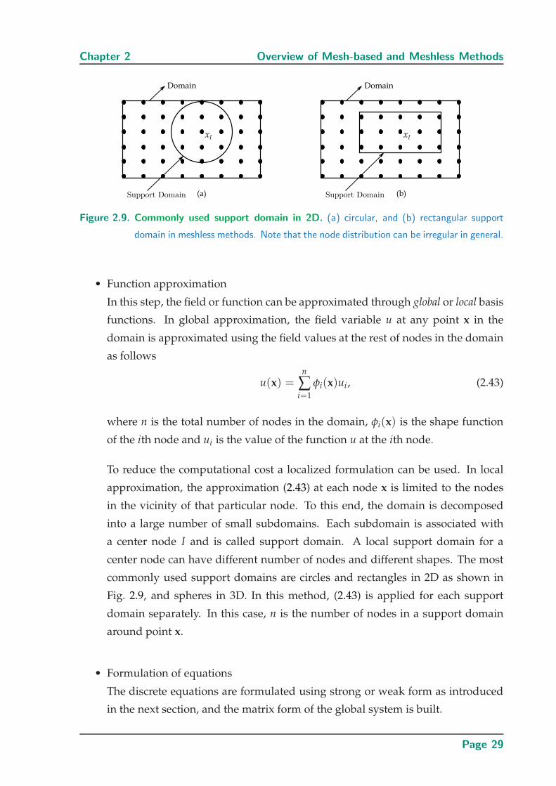
Chapter 2 Overview of Mesh-based and Meshless Methods
Figure 2.9. Commonly used support domain in 2D. (a) circular, and (b) rectangular support
domain in meshless methods. Note that the node distribution can be irregular in general.
• Function approximation
In this step, the field or function can be approximated through global or local basis
functions. In global approximation, the field variable u at any point x in the
domain is approximated using the field values at the rest of nodes in the domain
as follows
u(x) =n
∑i=1
φi(x)ui , (2.43)
where n is the total number of nodes in the domain, φi(x) is the shape function
of the ith node and ui is the value of the function u at the ith node.
To reduce the computational cost a localized formulation can be used. In local
approximation, the approximation (2.43) at each node x is limited to the nodes
in the vicinity of that particular node. To this end, the domain is decomposed
into a large number of small subdomains. Each subdomain is associated with
a center node I and is called support domain. A local support domain for a
center node can have different number of nodes and different shapes. The most
commonly used support domains are circles and rectangles in 2D as shown in
Fig. 2.9, and spheres in 3D. In this method, (2.43) is applied for each support
domain separately. In this case, n is the number of nodes in a support domain
around point x.
• Formulation of equations
The discrete equations are formulated using strong or weak form as introduced
in the next section, and the matrix form of the global system is built.
Page 29
2.3 Meshless Methods
• Solution of the equations
The matrix form of system of equations are solved and unknown coefficients are
obtained.
2.3.3 Classification of Meshless Methods
Many variations of meshless methods have been proposed over the past years. They
can be classified in different ways. In this subsection we classify them in two differ-
ent ways: classification based on formulation procedure and classification based on
function approximation schemes.
Classification based on Formulation Procedure
Numerical methods are generally classified into two large categories for solving PDEs
called direct approach (or strong form methods) and indirect approach (or weak form
methods). In direct approach the PDEs are discretized and solved directly. FDMs are in
this category. In indirect approach, PDEs with derivative boundary conditions are first
formulated with an alternative weak-form system of equations, usually in an integral
form. The approximate solution is then determined through a numerical integration
in the problem domain. FEM is an example of weak form methods. Both strong and
weak forms are used in meshless methods.
There are some important papers for meshless weak-form methods. Nayroles et al. [51]
applied the MLS approximation to the Galerkin weak-form and formulated the DEM.
Then DEM has been developed by Belytschko et al. [55] for mechanics problems. Since
then different meshless weak-form methods have been developed [73] such as: the
EFG method, RKPM, the MLPG [74], hp-cloud method [75], and the Partition of Unity
Finite Element Method (PUFEM) [61] as shown in Fig. 2.10.
In the strong-form meshless methods, which are also called meshless collocation meth-
ods, the PDEs are directly discretized at the field nodes using simple collocation tech-
niques. Some typical meshless strong-form methods are: General Finite Difference
Method (GFDM) [76, 77, 78, 79, 80], meshless collocation methods [81, 82, 83, 84, 85,
86], and the FPM [64, 87, 88]. The meshless strong-form methods are attractive since
they have a simple algorithm, high efficiency and they are truly meshless. However,
solving problems with derivative boundary conditions using strong-form methods
may suffer from instability. There are however some techniques to apply derivative
Page 30
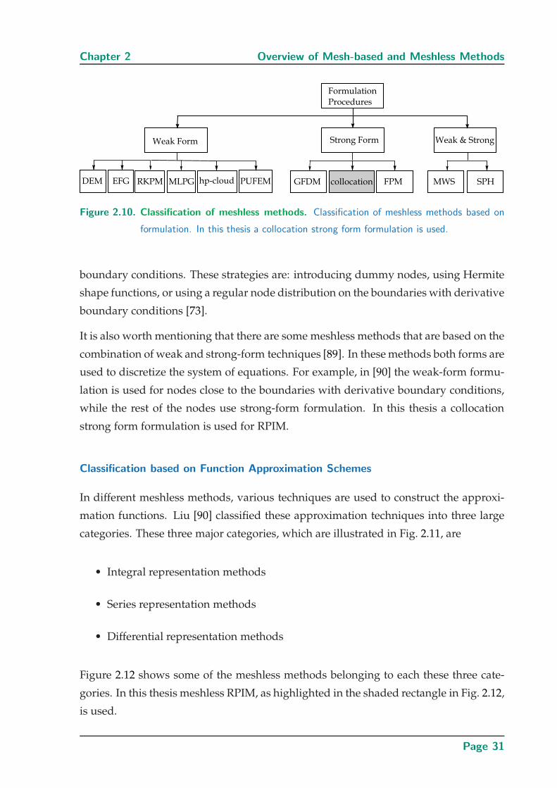
Chapter 2 Overview of Mesh-based and Meshless Methods
Figure 2.10. Classification of meshless methods. Classification of meshless methods based on
formulation. In this thesis a collocation strong form formulation is used.
boundary conditions. These strategies are: introducing dummy nodes, using Hermite
shape functions, or using a regular node distribution on the boundaries with derivative
boundary conditions [73].
It is also worth mentioning that there are some meshless methods that are based on the
combination of weak and strong-form techniques [89]. In these methods both forms are
used to discretize the system of equations. For example, in [90] the weak-form formu-
lation is used for nodes close to the boundaries with derivative boundary conditions,
while the rest of the nodes use strong-form formulation. In this thesis a collocation
strong form formulation is used for RPIM.
Classification based on Function Approximation Schemes
In different meshless methods, various techniques are used to construct the approxi-
mation functions. Liu [90] classified these approximation techniques into three large
categories. These three major categories, which are illustrated in Fig. 2.11, are
• Integral representation methods
• Series representation methods
• Differential representation methods
Figure 2.12 shows some of the meshless methods belonging to each these three cate-
gories. In this thesis meshless RPIM, as highlighted in the shaded rectangle in Fig. 2.12,
is used.
Page 31
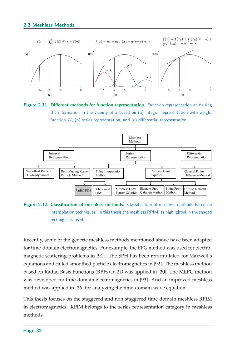
2.3 Meshless Methods
Figure 2.11. Different methods for function representation. Function representation at x using
the information in the vicinity of x based on (a) integral representation with weight
function W, (b) series representation, and (c) differential representation.
MeshlessMethods
Smoothed Particle Hydrodynamics
Moving LeastSquares
Point Interpolation Method
Radial PIM Polynomial PIM
Element-Free Galerkin Method
Finite Point Method
Integral Representation
Series Representation
Differential Representation
Reproducing Kernel Particle Method
General Finite Difference Method
Diffuse Element Method
Meshless LocalPetrov-Galerkin
Figure 2.12. Classification of meshless methods. Classification of meshless methods based on
interpolation techniques. In this thesis the meshless RPIM, as highlighted in the shaded
rectangle, is used.
Recently, some of the generic meshless methods mentioned above have been adapted
for time-domain electromagnetics. For example, the EFG method was used for electro-
magnetic scattering problems in [91]. The SPH has been reformulated for Maxwell’s
equations and called smoothed particle electromagnetics in [92]. The meshless method
based on Radial Basis Functions (RBFs) in 2D was applied in [20]. The MLPG method
was developed for time-domain electromagnetics in [93]. And an improved meshless
method was applied in [26] for analyzing the time-domain wave equation.
This thesis focuses on the staggered and non-staggered time-domain meshless RPIM
in electromagnetics. RPIM belongs to the series representation category in meshless
methods.
Page 32
Chapter 2 Overview of Mesh-based and Meshless Methods
2.3.4 Meshless Methods with Different Shape Functions
A common feature in all meshless methods is a weight function. Different weight
functions are used in various type of meshless methods. In fact, performance of the
method is fundamentally determined by the weight function. In local formulations,
the weight function is nonzero within the support domain, which is small compared
to the rest of the domain, and zero outside of the support domain.
In this section, different approximations with various weight functions for meshless
methods are described. To this end, the approximation of a function u(x) in a domain
Ω is considered. This domain includes a set of nodes xI , I = 1, . . . , nN and the function
value at node I is uI = u(xI).
Smooth Particle Hydrodynamics Approach (SPH)
In the SPH method [46, 47, 48, 94, 95, 96], an integral representation of a function is
used. In this method, the exact integral representation of a function u(x) at point x =
(x, y, z), which is given by
u(x) =∫ ∞
−∞u(ξ)δ(x − ξ)dξ, (2.44)
is approximated by
uh(x) =∫
Ωs
u(ξ)W(x − ξ, h)dξ, (2.45)
where δ(x) is the Dirac delta function, uh(x) is the approximation of function u(x),
W(x − ξ, h) is a kernel or weight or smoothing function, and h is the smoothing length
that controls the size of the support domain Ωs. The minimum requirements for the
weight function are compactness and unity conditions, which can be mathematically
described as follows
W(x − ξ, h) = 0, ∀ξ /∈ Ωs, (Compactness) (2.46a)∫
Ωs
W(x − ξ, h) = 1. (Unity) (2.46b)
However, additional conditions to the weight functions are often used to control sta-
bility and convergence of the solution in SPH. The required conditions for the weight
function are given in [48].
The discrete form of (2.45) can be obtained using the trapezoidal rule on the right-hand
side of the equation, which for 1D can be expressed as follows
uh(x) = ∑i∈Ωs
uiW(x − xi)∆xi. (2.47)
Page 33
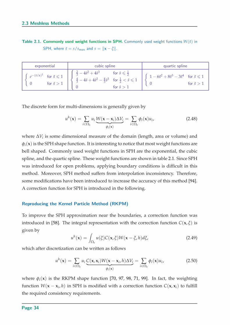
2.3 Meshless Methods
Table 2.1. Commonly used weight functions in SPH. Commonly used weight functions W(s) in
SPH, where s = s/smax and s = ‖x − ξ‖.
exponential cubic spline quartic spline
e−(s/α)2
for s 6 1
0 for s > 1
23 − 4s2 + 4s3 for s 6 1
243 − 4s + 4s2 − 4
3 s3 for 12 < s 6 1
0 for s > 1
1 − 6s2 + 8s3 − 3s4 for s 6 1
0 for s > 1
The discrete form for multi-dimensions is generally given by
uh(x) = ∑i∈Ωs
ui W(x − xi)∆Vi︸ ︷︷ ︸φi(x)
= ∑i∈Ωs
φi(x)ui , (2.48)
where ∆Vi is some dimensional measure of the domain (length, area or volume) and
φi(x) is the SPH shape function. It is interesting to notice that most weight functions are
bell shaped. Commonly used weight functions in SPH are the exponential, the cubic
spline, and the quartic spline. These weight functions are shown in table 2.1. Since SPH
was introduced for open problems, applying boundary conditions is difficult in this
method. Moreover, SPH method suffers from interpolation inconsistency. Therefore,
some modifications have been introduced to increase the accuracy of this method [94].
A correction function for SPH is introduced in the following.
Reproducing the Kernel Particle Method (RKPM)
To improve the SPH approximation near the boundaries, a correction function was
introduced in [58]. The integral representation with the correction function C(x, ξ) is
given by
uh(x) =∫
Ωs
u(ξ)C(x, ξ)W(x − ξ, h)dξ, (2.49)
which after discretization can be written as follows
uh(x) = ∑i∈Ωs
ui C(x, xi)W(x − xi, h)∆Vi︸ ︷︷ ︸φi(x)
= ∑i∈Ωs
φi(x)ui , (2.50)
where φi(x) is the RKPM shape function [70, 97, 98, 71, 99]. In fact, the weighting
function W(x − xi, h) in SPH is modified with a correction function C(x, xi) to fulfill
the required consistency requirements.
Page 34
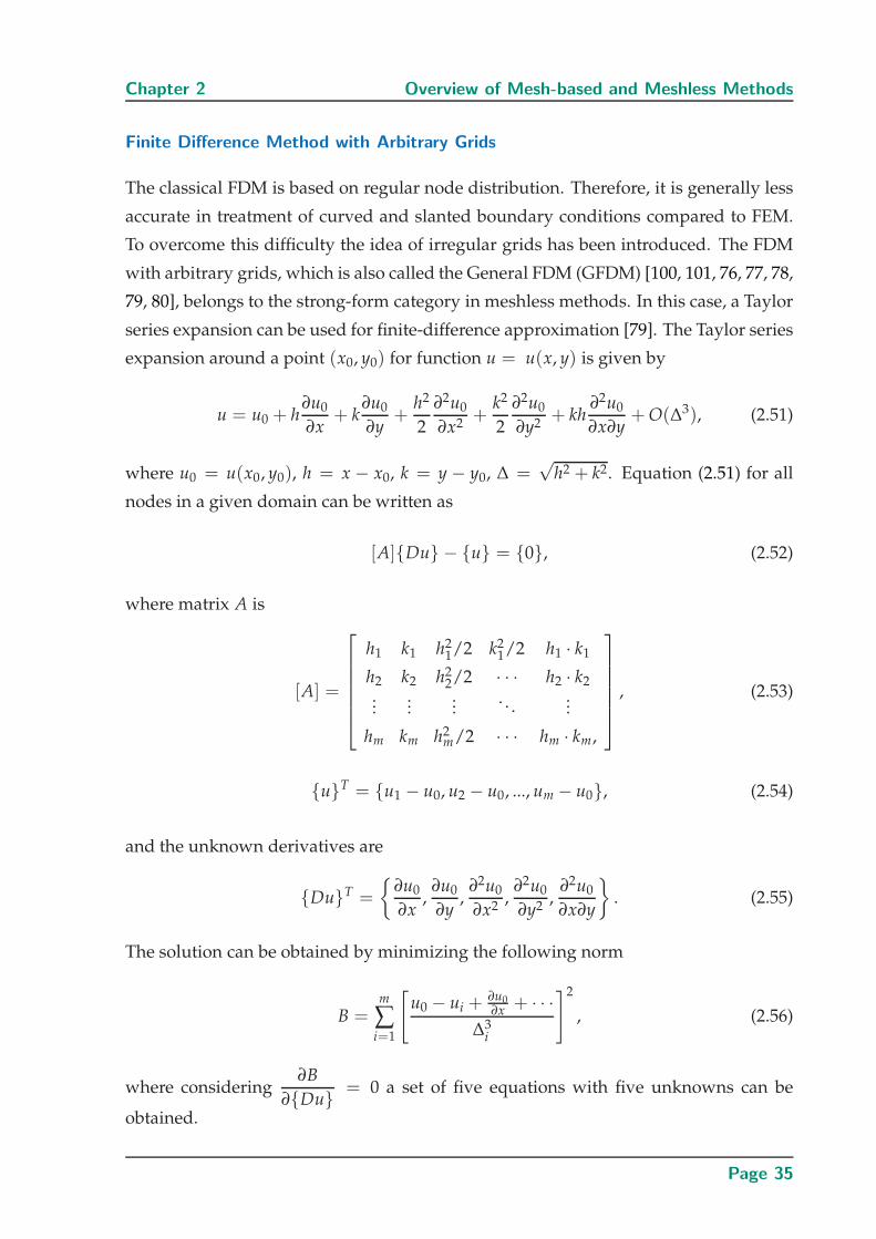
Chapter 2 Overview of Mesh-based and Meshless Methods
Finite Difference Method with Arbitrary Grids
The classical FDM is based on regular node distribution. Therefore, it is generally less
accurate in treatment of curved and slanted boundary conditions compared to FEM.
To overcome this difficulty the idea of irregular grids has been introduced. The FDM
with arbitrary grids, which is also called the General FDM (GFDM) [100, 101, 76, 77, 78,
79, 80], belongs to the strong-form category in meshless methods. In this case, a Taylor
series expansion can be used for finite-difference approximation [79]. The Taylor series
expansion around a point (x0, y0) for function u = u(x, y) is given by
u = u0 + h∂u0
∂x+ k
∂u0
∂y+
h2
2
∂2u0
∂x2+
k2
2
∂2u0
∂y2+ kh
∂2u0
∂x∂y+ O(∆3), (2.51)
where u0 = u(x0, y0), h = x − x0, k = y − y0, ∆ =√
h2 + k2. Equation (2.51) for all
nodes in a given domain can be written as
[A]Du − u = 0, (2.52)
where matrix A is
[A] =
h1 k1 h21/2 k2
1/2 h1 · k1
h2 k2 h22/2 · · · h2 · k2
......
.... . .
...
hm km h2m/2 · · · hm · km,
, (2.53)
uT = u1 − u0, u2 − u0, ..., um − u0, (2.54)
and the unknown derivatives are
DuT =
∂u0
∂x,
∂u0
∂y,
∂2u0
∂x2,
∂2u0
∂y2,
∂2u0
∂x∂y
. (2.55)
The solution can be obtained by minimizing the following norm
B =m
∑i=1
[u0 − ui +
∂u0∂x + · · ·
∆3i
]2
, (2.56)
where considering∂B
∂Du = 0 a set of five equations with five unknowns can be
obtained.
Page 35
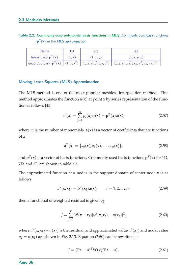
2.3 Meshless Methods
Table 2.2. Commonly used polynomial basis functions in MLS. Commonly used basis functions
pT(x) in the MLS approximation.
Name 1D 2D 3D
linear basis pT(x) (1, x) (1, x, y) (1, x, y, z)
quadratic basis pT(x) (1, x, x2) (1, x, y, x2, xy, y2) (1, x, y, z, x2, xy, y2, yz, xz, z2)
Moving Least Squares (MLS) Approximation
The MLS method is one of the most popular meshless interpolation method. This
method approximates the function u(x) at point x by series representation of the func-
tion as follows [45]
uh(x) =m
∑j=1
pj(x)aj(x) = pT(x)a(x), (2.57)
where m is the number of monomials, a(x) is a vector of coefficients that are functions
of x
aT(x) = a0(x), a1(x), . . . , am(x), (2.58)
and pT(x) is a vector of basis functions. Commonly used basis functions pT(x) for 1D,
2D, and 3D are shown in table 2.2.
The approximated function at n nodes in the support domain of center node x is as
follows
uh(x, xI) = pT(xI)a(x), I = 1, 2, . . . , n (2.59)
then a functional of weighted residual is given by
J =n
∑I=1
W(x − xI)[uh(x, xI)− u(xI)]
2, (2.60)
where uh(x, xI)− u(xI ) is the residual, and approximated value uh(xI) and nodal value
uI = u(xI) are shown in Fig. 2.13. Equation (2.60) can be rewritten as
J = (Pa − u)TW(x)(Pa − u), (2.61)
Page 36
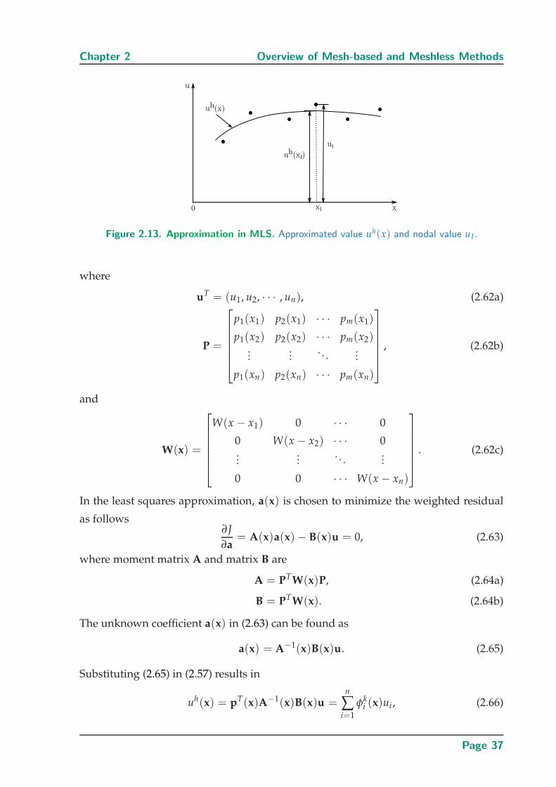
Chapter 2 Overview of Mesh-based and Meshless Methods
Figure 2.13. Approximation in MLS. Approximated value uh(x) and nodal value uI .
where
uT = (u1, u2, · · · , un), (2.62a)
P =
p1(x1) p2(x1) · · · pm(x1)
p1(x2) p2(x2) · · · pm(x2)...
.... . .
...
p1(xn) p2(xn) · · · pm(xn)
, (2.62b)
and
W(x) =
W(x − x1) 0 · · · 0
0 W(x − x2) · · · 0...
.... . .
...
0 0 · · · W(x − xn)
. (2.62c)
In the least squares approximation, a(x) is chosen to minimize the weighted residual
as follows∂J
∂a= A(x)a(x)− B(x)u = 0, (2.63)
where moment matrix A and matrix B are
A = PTW(x)P, (2.64a)
B = PTW(x). (2.64b)
The unknown coefficient a(x) in (2.63) can be found as
a(x) = A−1(x)B(x)u. (2.65)
Substituting (2.65) in (2.57) results in
uh(x) = pT(x)A−1(x)B(x)u =n
∑i=1
φki (x)ui , (2.66)
Page 37
2.3 Meshless Methods
where the shape function is
φk = [φk1(x), · · · , φk
n(x)] = pT(x)A−1(x)B(x), (2.67)
and k is the order of the polynomial basis function. For k = 0 the shape function is
called Shepard function [102].
To improve the efficiency of the MLS method, a developed interpolation scheme has
been introduced in [103].
Point Interpolation Method (PIM)
The point interpolation method is in the series representation category. There are two
types of point interpolation method based on different forms of basis functions
• Polynomial PIM
• Radial PIM (RPIM)
The polynomial PIM was introduced as an alternative to MLS in [104]. In the polyno-
mial PIM, approximation function is defined by
uh(x) =m
∑i=1
pi(x)ai = pT(x)a, (2.68)
where pi(x) is the monomials basis function, m is the number of monomials, and ai is
the unknown coefficients as follows
a = a1, a2, . . . , amT.
The coefficients ai can be found through point matching technique. The value of u at
ith node is given by
ui = pT(xi)a. i = 1, 2, . . . , n (2.69)
Vector pT(x) contains a polynomial basis function with order of p, which can be ex-
pressed for 1D as follows
pT(x) = 1, x, x2, · · · , xp, (2.70)
and for 2D as follows
pT(x) = 1, x, y, x2, xy, y2, · · · , xp, yp. (2.71)
Page 38
Chapter 2 Overview of Mesh-based and Meshless Methods
Equation (2.69) results in following n equations for n nodes in the domain
u1 =m
∑i=1
pi(x1)ai = a1 + a2 p2(x1) + · · ·+ am pm(x1), (2.72a)
u2 =m
∑i=1
pi(x2)ai = a1 + a2 p2(x2) + · · ·+ am pm(x2), (2.72b)
... (2.72c)
un =m
∑i=1
pi(xn)ai = a1 + a2 p2(xn) + · · ·+ am pm(xn), (2.72d)
which can be expressed by the following matrix form
U0 = Pa, (2.73)
where U0 holds the values of the function at all the n nodes
U0 = u1, u2, . . . , unT, (2.74)
and P is given by
P =
pT(x1)
pT(x2)...
pT(xn)
. (2.75)
The matrix P is a square matrix since n = m in the PIM [73]. So, the unknown coeffi-
cients a can be obtained as
a = P−1U0. (2.76)
Substituting (2.76) in (2.69), and considering n = m result in
u(x) = PT(x)P−1U0 =n
∑i=1
φi(x)ui = ΦT(x)U0, (2.77)
where Φ(x) is a vector of shape functions. Polynomial PIM suffers from singularity
problem in the interpolation process. To avoid the singular matrix in polynomial PIM,
the RBFs were used and RPIM was introduced. RPIM will be described in the next
chapter in more detail.
2.4 Summary
Numerical methods can be broadly classified into mesh-based and meshless methods.
This chapter has first reviewed some mesh-based methods, e.g., FDTD and FEM, in
Page 39

2.4 Summary
the perspective of comparing their properties with meshless methods. The difficulties
associated to mesh-based methods have been discussed briefly and meshless methods
were introduced as an alternative approach. Also, different meshless methods have
been introduced and categorized based on two different classification schemes. More-
over, meshless methods with various basis functions have been discussed including
PIM, as applied in the rest of this thesis. The next chapter will discuss PIM based on
RBFs in more detail.
Page 40
Chapter 3
Radial Point InterpolationMethod
THIS chapter reviews the concept and the fundamental theory of
the Radial Point Interpolation Method (RPIM) as basic knowledge
for the other chapters of this thesis. This interpolation method is
introduced first for globally supported basis functions and then a localized
approach using locally supported basis functions is explained. In the sec-
ond part of this chapter, different local basis functions are considered, with
in particular a comparison of the Gaussian and Wendland basis functions
for use in RPIM. It is shown that the Gaussian basis functions are more ap-
propriate for the interpolation in small support domains, whereas Wend-
land basis functions are more accurate for larger support domains.
Page 41
3.1 Introduction
3.1 Introduction
As shown in the previous chapter, the Point Interpolation Method (PIM) approximates
a function at a certain location by interpolation of the function values in scattered nodes
within a considered domain. One type of PIM is the polynomial PIM [104]. Using
polynomial basis functions is simple and accurate, but may result in singular matrices
in the process of interpolation [105, 85]. To overcome the singularity problem, the
radial PIM which uses Radial Basis Functions (RBFs) was introduced in [85].
Interpolating with RBFs is an appropriate method for interpolating scattered data. A
RBF at a particular node xi is a function of the distance between the node xi and inter-
polating point x. Using RBFs for the interpolation has many advantages [106], such as
reproducing sufficiently smooth functions with high accuracy, and straightforward ex-
tension to higher-dimentional formulations. It is shown in [107] that RBF interpolation
is one of the best scheme among various 2D interpolation methods.
The RBFs have been used in various applications including geodesy, geophysics, sur-
veying and mapping, photogrammetry, remote sensing, signal processing, geography,
and hydrology [108, 109]. Importantly, Kansa [110, 81] introduced a method for solv-
ing Partial Differential Equations (PDEs) using RBFs. Since then, the RBFs have been
increasingly used in the numerical solution of PDEs [111, 112, 113, 114, 115, 116, 117,
118, 119]. RBFs-based methods are a viable alternative to more traditional methods,
such as finite differences or finite elements, and have several attractive features, such
as the flexibility in the choice of node locations and a fast convergence (exponential for
some cases).
RBFs can be used in the formulation of PIM and the method is called Radial Point
Interpolation Method (RPIM) [85]. The RPIM will be introduced in this chapter.
3.2 Interpolation Method
Among different types of meshless methods based on different interpolation tech-
niques, the RPIM has been selected for investigation in this thesis. In this interpolation
method, global or local basis functions can be used, as introduced in the following.
Page 42
Chapter 3 Radial Point Interpolation Method
3.2.1 Global Basis Functions
In the global RPIM, the field value at a given position x can be interpolated based on
the field values at N node locations scattered in the entire computational domain. This
is realized as follows using RBFs
uh(x) =N
∑n=1
anrn(x), (3.1)
where an represent unknown coefficients, N is the number of nodes in the domain,
and rn(x) are the RBFs, which will be discussed later in this chapter. To make sure
that the interpolation can reconstruct a linear function and increase the accuracy of the
approximation [90], this interpolation can be extended with monomial basis functions
pm(x) as follows
uh(x) =N
∑n=1
anrn(x) +M
∑m=1
bmpm(x) = RT(x)a + PT(x)b, (3.2)
where a and b are unknown coefficients, which can be expressed in vectorial form as
aT =(
a1, a2, · · · , aN
)1×N
(3.3)
bT =(
b1, b2, · · · , bM
)1×M
. (3.4)
The vector PT(x) contains polynomial basis function with M terms as shown in the
previous chapter in table 2.2
PT(x) = [p1(x), p2(x), · · · , pm(x)] = [1, x, y, · · · ], (3.5)
and the vector RT(x), which contains the RBFs rn(x), can be expressed as follows
RT(x) = [r1(x), r2(x), ..., rN(x)]. (3.6)
As will be discussed in the next section, there are different types of RBFs that can be
chosen as rn(x).
The unknowns coefficients a and b in (3.2) can be determined in a pre-processing step
as follows: Applying (3.2) for all N nodes in the computational domain results in the
following expression
Ue = R0a + P0b, (3.7)
Page 43
3.2 Interpolation Method
where Ue = (u1, u2, ..., uN)T holds the field values at N node locations. The matrices
R0 and P0 are then defined as follows
R0 =
r1(x1) r2(x1) · · · rN(x1)
r1(x2) r2(x2) · · · rN(x2)...
.... . .
...
r1(xN) r2(xN) · · · rN(xN)
N×N
, (3.8)
and
P0 =
p1(x1) p2(x1) · · · pM(x1)
p1(x2) p2(x2) · · · pM(x2)...
.... . .
...
p1(xN) p2(xN) · · · pM(xN)
N×M
. (3.9)
The equation (3.2) has N + M variables. The additional M equations can be considered
using the constraint condition P0Ta = 0 [90, 73]. Considering this condition and (3.7)
the following matrix form can be given(
R0 P0
PT0 0
)
︸ ︷︷ ︸G
(a
b
)=
(Ue
0
), (3.10)
where the condition P0Ta = 0 results in a square (N + M)× (N + M) matrix G. There-
fore, the unknown coefficients can be determined as(
a
b
)= G−1
(Ue
0
). (3.11)
Substituting (3.11) in (3.2) gives
uh(x) =[
RT(x) PT(x)]
G−1
(Ue
0
)= Φ(x)Ue , (3.12)
where Φ(x) = [φ1(x), φ2(x), ..., φN(x)] is called shape function. Using this shape func-
tion, the interpolated value for a function, i.e., u(x) and its space derivatives can be
re-written as
uh(x) = [φ1(x), φ2(x), ..., φN(x)]Ue , (3.13a)
∂uh(x)
∂k= [
∂φ1(x)
∂k,
∂φ2(x)
∂k, ...,
∂φN(x)
∂k]Ue, (3.13b)
∂2uh(x)
∂k2= [
∂2φ1(x)
∂k2,
∂2φ2(x)
∂k2, ...,
∂2φN(x)
∂k2]Ue. (3.13c)
Note that these approximations of the space derivatives will be used for the spatial
discretization of PDEs in the meshless RPIM method, as described later in this thesis.
Page 44
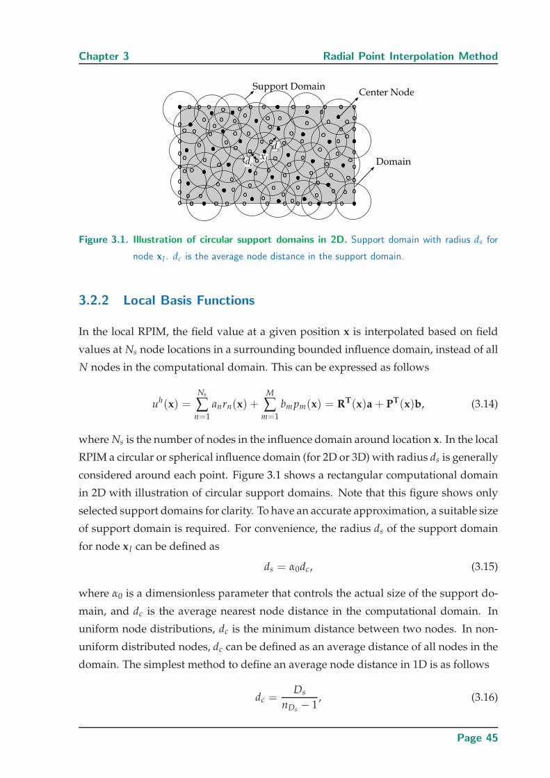
Chapter 3 Radial Point Interpolation Method
Figure 3.1. Illustration of circular support domains in 2D. Support domain with radius ds for
node xI . dc is the average node distance in the support domain.
3.2.2 Local Basis Functions
In the local RPIM, the field value at a given position x is interpolated based on field
values at Ns node locations in a surrounding bounded influence domain, instead of all
N nodes in the computational domain. This can be expressed as follows
uh(x) =Ns
∑n=1
anrn(x) +M
∑m=1
bmpm(x) = RT(x)a + PT(x)b, (3.14)
where Ns is the number of nodes in the influence domain around location x. In the local
RPIM a circular or spherical influence domain (for 2D or 3D) with radius ds is generally
considered around each point. Figure 3.1 shows a rectangular computational domain
in 2D with illustration of circular support domains. Note that this figure shows only
selected support domains for clarity. To have an accurate approximation, a suitable size
of support domain is required. For convenience, the radius ds of the support domain
for node xI can be defined as
ds = α0dc, (3.15)
where α0 is a dimensionless parameter that controls the actual size of the support do-
main, and dc is the average nearest node distance in the computational domain. In
uniform node distributions, dc is the minimum distance between two nodes. In non-
uniform distributed nodes, dc can be defined as an average distance of all nodes in the
domain. The simplest method to define an average node distance in 1D is as follows
dc =Ds
nDs − 1, (3.16)
Page 45
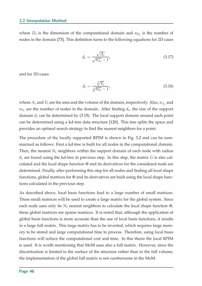
3.2 Interpolation Method
where Ds is the dimension of the computational domain and nDs is the number of
nodes in the domain [73]. This definition turns to the following equations for 2D cases
dc =
√As√
nAs − 1, (3.17)
and for 3D cases
dc =3√
Vs
3√
nVs − 1, (3.18)
where As and Vs are the area and the volume of the domain, respectively. Also, nAsand
nVs are the number of nodes in the domain. After finding dc, the size of the support
domain ds can be determined by (3.15). The local support domain around each point
can be determined using a kd-tree data structure [120]. This tree splits the space and
provides an optimal search strategy to find the nearest neighbors for a point.
The procedure of the locally supported RPIM is shown in Fig. 3.2 and can be sum-
marized as follows: First a kd-tree is built for all nodes in the computational domain.
Then, the nearest Ns neighbors within the support domain of each node with radius
ds are found using the kd-tree in previous step. In this step, the matrix G is also cal-
culated and the local shape function Φ and its derivatives for the considered node are
determined. Finally, after performing this step for all nodes and finding all local shape
functions, global matrices for Φ and its derivatives are built using the local shape func-
tions calculated in the previous step.
As described above, local basis functions lead to a large number of small matrices.
These small matrices will be used to create a large matrix for the global system. Since
each node uses only its Ns nearest neighbors to calculate the local shape function Φ,
these global matrices are sparse matrices. It is noted that, although the application of
global basis functions is more accurate than the use of local basis functions, it results
in a large full matrix. This large matrix has to be inverted, which requires large mem-
ory to be stored and large computational time to process. Therefore, using local basis
functions will reduce the computational cost and time. In this thesis the local RPIM
is used. It is worth mentioning that MoM uses also a full matrix. However, since the
discretization is limited to the surface of the structure rather than in the full volume,
the implementation of the global full matrix is not cumbersome in the MoM.
Page 46
Chapter 3 Radial Point Interpolation Method
Figure 3.2. Flowchart of the localized supported RPIM. The procedure for the computing shape
functions and its spatial derivatives using local RBFs.
3.3 Different Radial Basis Functions (RBFs)
A RBF is a function of Euclidean distance, which in 2D can be written as
ρ =√(x − x0)2 + (y − y0)2, (3.19)
where (x0, y0) is a center node position in a support domain. There are different types
of RBFs, and a non-exhaustive list can be found in the table 3.1 [121]. In this section,
two types of basis functions, which are Gaussian and Wendland basis functions, are
studied and compared for RPIM applied in different support domain sizes.
3.3.1 Gaussian and Wendland Basis Functions
Here, Gaussian and Wendland basis functions are studied for RPIM with two different
support domain sizes ds = 3∆x and ds = 5∆x. The following Gaussian basis function
rn(x) = exp
(−α
(ρ
ds
)2)
, (3.20)
is considered as first type of basis function. Gaussian basis functions have in princi-
ple an infinite extent, and need to be truncated for application in a compact support
domain. In (3.20), ρ = |x − xn| is the Euclidean distance and α is called the shape
Page 47
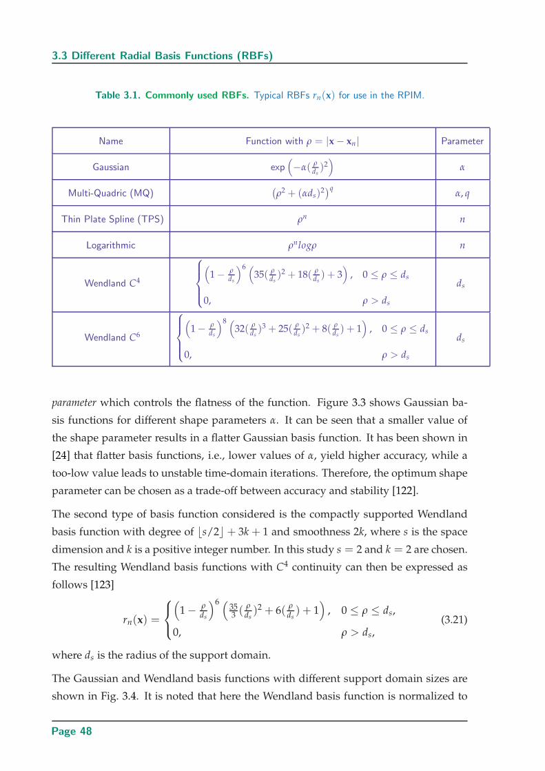
3.3 Different Radial Basis Functions (RBFs)
Table 3.1. Commonly used RBFs. Typical RBFs rn(x) for use in the RPIM.
Name Function with ρ = |x − xn| Parameter
Gaussian exp(−α( ρ
ds)2)
α
Multi-Quadric (MQ)(ρ2 + (αds)2
)qα, q
Thin Plate Spline (TPS) ρn n
Logarithmic ρnlogρ n
Wendland C4
(1 − ρ
ds
)6 (35( ρ
ds)2 + 18( ρ
ds) + 3
), 0 ≤ ρ ≤ ds
0, ρ > ds
ds
Wendland C6
(1 − ρ
ds
)8 (32( ρ
ds)3 + 25( ρ
ds)2 + 8( ρ
ds) + 1
), 0 ≤ ρ ≤ ds
0, ρ > ds
ds
parameter which controls the flatness of the function. Figure 3.3 shows Gaussian ba-
sis functions for different shape parameters α. It can be seen that a smaller value of
the shape parameter results in a flatter Gaussian basis function. It has been shown in
[24] that flatter basis functions, i.e., lower values of α, yield higher accuracy, while a
too-low value leads to unstable time-domain iterations. Therefore, the optimum shape
parameter can be chosen as a trade-off between accuracy and stability [122].
The second type of basis function considered is the compactly supported Wendland
basis function with degree of ⌊s/2⌋ + 3k + 1 and smoothness 2k, where s is the space
dimension and k is a positive integer number. In this study s = 2 and k = 2 are chosen.
The resulting Wendland basis functions with C4 continuity can then be expressed as
follows [123]
rn(x) =
(1 − ρ
ds
)6 (353 (
ρds)2 + 6(
ρds) + 1
), 0 ≤ ρ ≤ ds,
0, ρ > ds,(3.21)
where ds is the radius of the support domain.
The Gaussian and Wendland basis functions with different support domain sizes are
shown in Fig. 3.4. It is noted that here the Wendland basis function is normalized to
Page 48
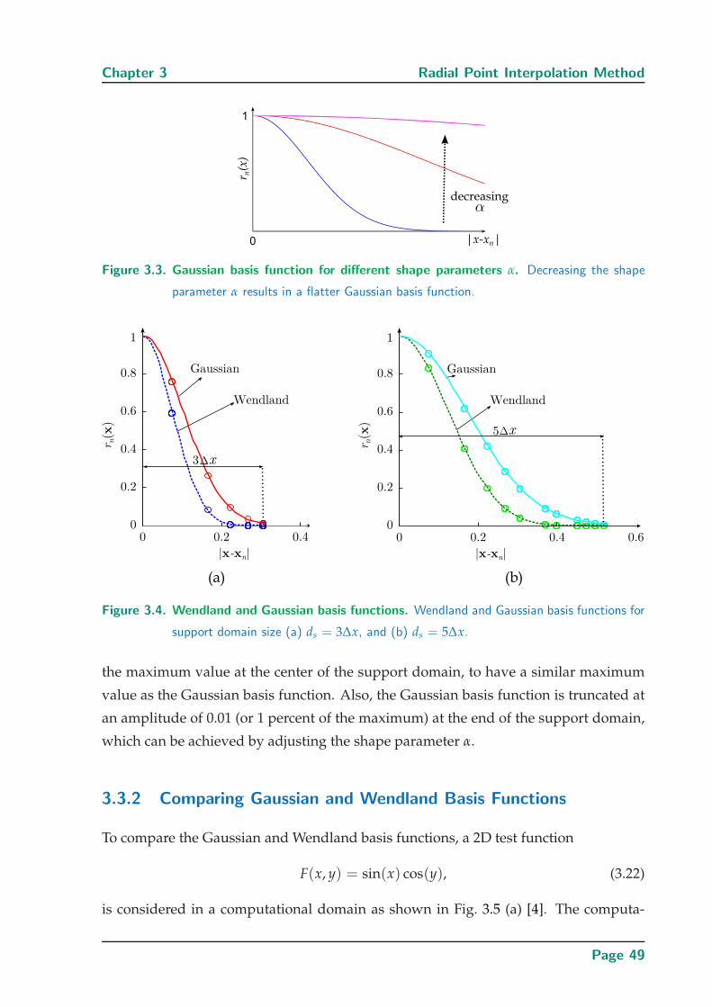
Chapter 3 Radial Point Interpolation Method
Figure 3.3. Gaussian basis function for different shape parameters α. Decreasing the shape
parameter α results in a flatter Gaussian basis function.
Figure 3.4. Wendland and Gaussian basis functions. Wendland and Gaussian basis functions for
support domain size (a) ds = 3∆x, and (b) ds = 5∆x.
the maximum value at the center of the support domain, to have a similar maximum
value as the Gaussian basis function. Also, the Gaussian basis function is truncated at
an amplitude of 0.01 (or 1 percent of the maximum) at the end of the support domain,
which can be achieved by adjusting the shape parameter α.
3.3.2 Comparing Gaussian and Wendland Basis Functions
To compare the Gaussian and Wendland basis functions, a 2D test function
F(x, y) = sin(x) cos(y), (3.22)
is considered in a computational domain as shown in Fig. 3.5 (a) [4]. The computa-
Page 49
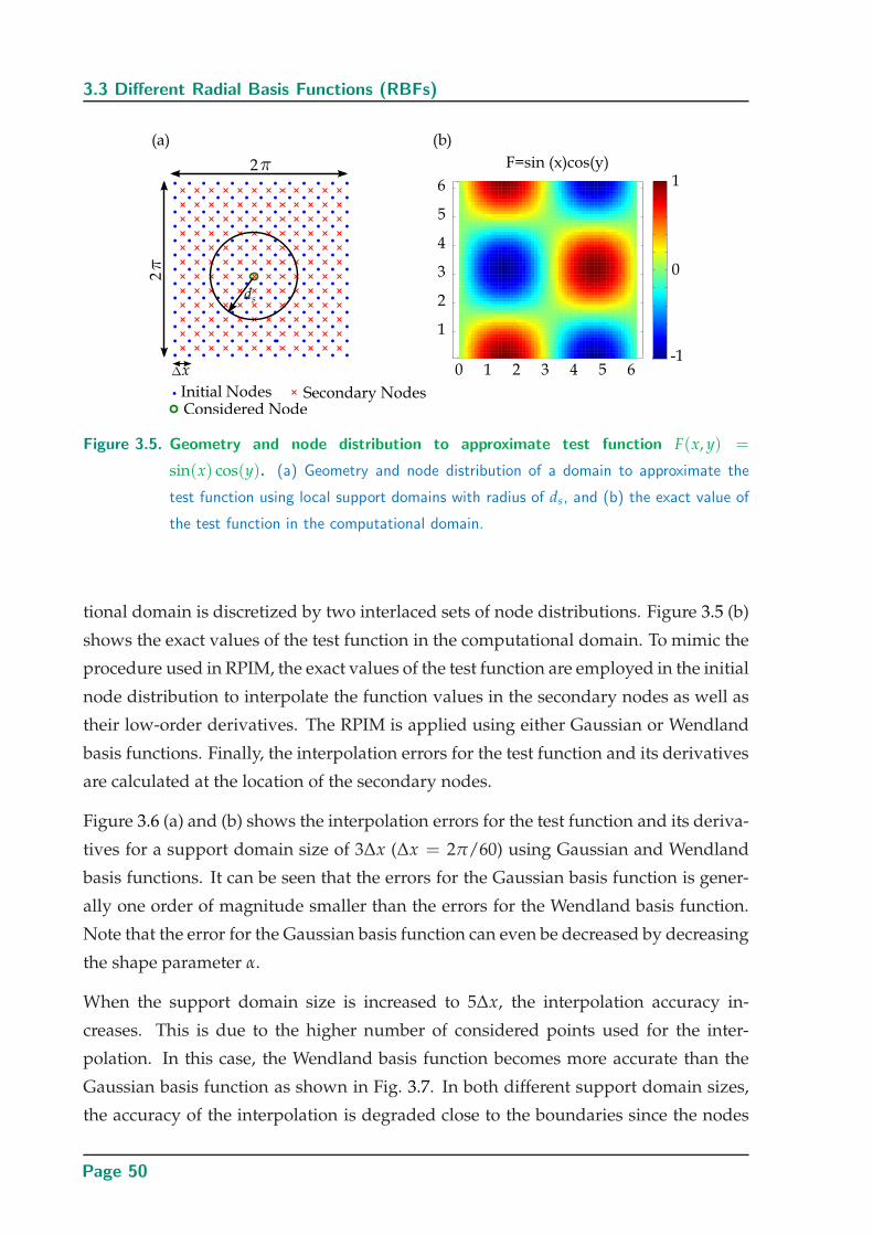
3.3 Different Radial Basis Functions (RBFs)
Figure 3.5. Geometry and node distribution to approximate test function F(x, y) =
sin(x) cos(y). (a) Geometry and node distribution of a domain to approximate the
test function using local support domains with radius of ds, and (b) the exact value of
the test function in the computational domain.
tional domain is discretized by two interlaced sets of node distributions. Figure 3.5 (b)
shows the exact values of the test function in the computational domain. To mimic the
procedure used in RPIM, the exact values of the test function are employed in the initial
node distribution to interpolate the function values in the secondary nodes as well as
their low-order derivatives. The RPIM is applied using either Gaussian or Wendland
basis functions. Finally, the interpolation errors for the test function and its derivatives
are calculated at the location of the secondary nodes.
Figure 3.6 (a) and (b) shows the interpolation errors for the test function and its deriva-
tives for a support domain size of 3∆x (∆x = 2π/60) using Gaussian and Wendland
basis functions. It can be seen that the errors for the Gaussian basis function is gener-
ally one order of magnitude smaller than the errors for the Wendland basis function.
Note that the error for the Gaussian basis function can even be decreased by decreasing
the shape parameter α.
When the support domain size is increased to 5∆x, the interpolation accuracy in-
creases. This is due to the higher number of considered points used for the inter-
polation. In this case, the Wendland basis function becomes more accurate than the
Gaussian basis function as shown in Fig. 3.7. In both different support domain sizes,
the accuracy of the interpolation is degraded close to the boundaries since the nodes
Page 50
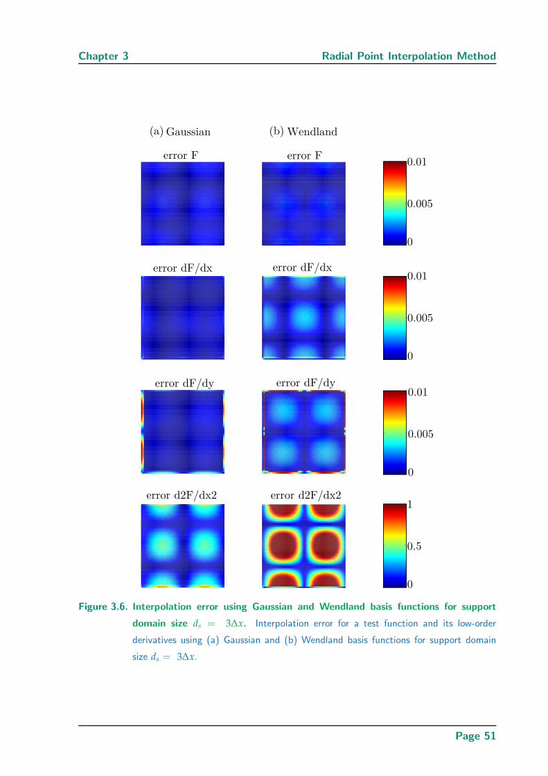
Chapter 3 Radial Point Interpolation Method
Figure 3.6. Interpolation error using Gaussian and Wendland basis functions for support
domain size ds = 3∆x. Interpolation error for a test function and its low-order
derivatives using (a) Gaussian and (b) Wendland basis functions for support domain
size ds = 3∆x.
Page 51
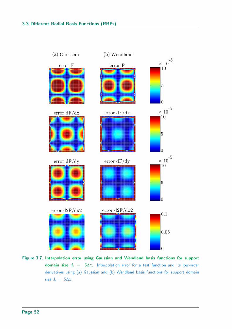
3.3 Different Radial Basis Functions (RBFs)
Figure 3.7. Interpolation error using Gaussian and Wendland basis functions for support
domain size ds = 5∆x. Interpolation error for a test function and its low-order
derivatives using (a) Gaussian and (b) Wendland basis functions for support domain
size ds = 5∆x.
Page 52
Chapter 3 Radial Point Interpolation Method
used for interpolation are limited to the computational domain. The implementation
of appropriate boundary conditions would mitigate this effect.
For application in computational electromagnetics using meshless RPIM, the first-order
spatial derivatives for the electric and magnetic fields in Maxwell’s curl equations have
to be approximated through basis functions. Alternatively, second-order derivatives
can be utilized for solving the wave equations. In both cases, choosing more accurate
basis functions allows to decrease approximation errors in the computational domain.
It is worth mentioning that in time-domain algorithms, small support domains are pre-
ferred because of a higher computational efficiency of sparse matrices instead of full
matrices. To this aim, truncated Gaussian basis functions appear to be better suited to
get more accurate results in the small support domain.
3.4 Conclusion
The RPIM has been introduced in this chapter. In this method, a combination of radial
and polynomial basis functions is used to obtain a highly accurate interpolation of a
function and its associated derivatives. The variations of this interpolation method
using globally and locally supported domain basis functions have been distinguished.
Also, the general procedure for implementing local RPIM has been summarized. In
the local RPIM only nodes in the local support domain are used for the interpolation
at a particular node. Therefore, local RPIM reduces the computational cost and time.
In the second part, two different types of RBFs typically used in the meshless RPIM
have been studied. The interpolation errors for a test function and its derivatives have
been calculated using Gaussian and Wendland basis functions with different support
domain sizes. It has been shown that the Gaussian basis functions have smaller errors
for interpolation of a function and its derivatives in small support domains. However,
as the size of the support domain is increased, the use of the Wendland basis functions
gradually allows to achieve higher interpolation accuracy. The application of local
RPIM in time-domain electromagnetics will be shown in the next chapters. Since small
support domains are preferred in time-domain methods, the truncated Gaussian basis
functions, which have a better accuracy in this case, will be used.
Page 53

Page 54
Chapter 4
Staggered Meshless RPIM
THIS chapter is dedicated to the staggered meshless Radial Point
Interpolation Method (RPIM) in electromagnetics. In the first part
of the chapter, the update equations are derived for the staggered
electric and magnetic fields in the framework of the first-order meshless
RPIM. Moreover, the truncation of the computational domain is introduced
and the implementation of a Uniaxial Perfectly Matched Layer (UPML) is
explained as the most popular technique to absorb the energy in the sim-
ulation of unbounded problems. The update equations for the staggered
meshless RPIM are then modified to include a novel implementation of
UPML. It is also shown that UPML suffers from late-time instability that
can be solved by introducing small loss factors in the UPMLs after almost
all the energy in the computational domain is absorbed. Finally, in this
chapter some of the properties and capabilities of meshless methods are
demonstrated through selected numerical examples.
Page 55
4.1 Staggered Meshless RPIM in Electromagnetics
4.1 Staggered Meshless RPIM in Electromagnetics
In the staggered meshless Radial Point Interpolation Method (RPIM), the first-order
spatial derivatives in the Maxwell’s curl equations (1.1) are discretized through the
RPIM. The curl operators in the Maxwell’s equations are defined as
∇× E =
∂∂x∂
∂y∂∂z
×
Ex
Ey
Ez
=
∂Ez∂y − ∂Ey
∂z∂Ex∂z − ∂Ez
∂x∂Ey
∂x − ∂Ex∂y
, (4.1)
and
∇× H =
∂∂x∂
∂y∂∂z
×
Hx
Hy
Hz
=
∂Hz∂y − ∂Hy
∂z∂Hx∂z − ∂Hz
∂x∂Hy
∂x − ∂Hx∂y
. (4.2)
Considering the curl definition, the following time-domain equations can be obtained
from Maxwell’s curl equations in 3D
∂Hx
∂t=
1
µ(
∂Ey
∂z− ∂Ez
∂y), (4.3a)
∂Hy
∂t=
1
µ(
∂Ez
∂x− ∂Ex
∂z), (4.3b)
∂Hz
∂t=
1
µ(
∂Ex
∂y− ∂Ey
∂x), (4.3c)
and
∂Ex
∂t=
1
ǫ(
∂Hz
∂y− ∂Hy
∂z− Jx), (4.4a)
∂Ey
∂t=
1
ǫ(
∂Hx
∂z− ∂Hz
∂x− Jy), (4.4b)
∂Ez
∂t=
1
ǫ(
∂Hy
∂x− ∂Hx
∂y− Jz). (4.4c)
It is noted that there are both time and space derivatives in the above equations. To
implement the staggered meshless RPIM these equations have to be discretized. The
discretization of time and space as well as the path for obtaining the update equations
for the staggered meshless RPIM are described in the following subsections.
4.1.1 Time Discretization
The time derivatives in the time-domain meshless RPIM method can be approximated
by central finite differences in a leapfrog time-stepping scheme similarly as commonly
Page 56
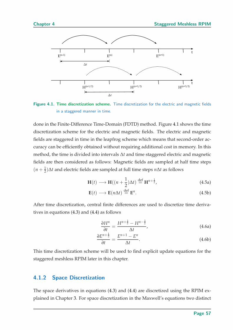
Chapter 4 Staggered Meshless RPIM
Figure 4.1. Time discretization scheme. Time discretization for the electric and magnetic fields
in a staggered manner in time.
done in the Finite-Difference Time-Domain (FDTD) method. Figure 4.1 shows the time
discretization scheme for the electric and magnetic fields. The electric and magnetic
fields are staggered in time in the leapfrog scheme which means that second-order ac-
curacy can be efficiently obtained without requiring additional cost in memory. In this
method, the time is divided into intervals ∆t and time staggered electric and magnetic
fields are then considered as follows: Magnetic fields are sampled at half time steps
(n + 12)∆t and electric fields are sampled at full time steps n∆t as follows
H(t) −→ H((n +1
2)∆t)
def= Hn+ 1
2 , (4.5a)
E(t) −→ E(n∆t)def= En. (4.5b)
After time discretization, central finite differences are used to discretize time deriva-
tives in equations (4.3) and (4.4) as follows
∂Hn
∂t=
Hn+ 12 − Hn− 1
2
∆t, (4.6a)
∂En+ 12
∂t=
En+1 − En
∆t. (4.6b)
This time discretization scheme will be used to find explicit update equations for the
staggered meshless RPIM later in this chapter.
4.1.2 Space Discretization
The space derivatives in equations (4.3) and (4.4) are discretized using the RPIM ex-
plained in Chapter 3. For space discretization in the Maxwell’s equations two distinct
Page 57
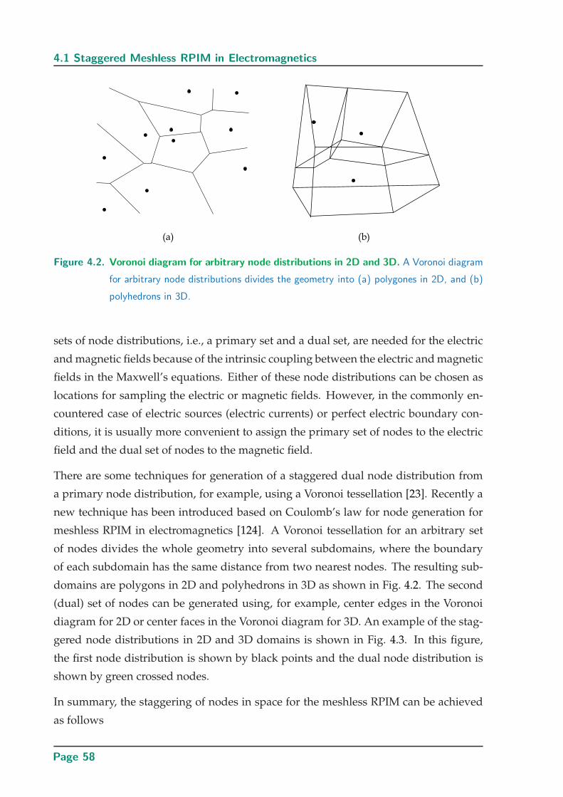
4.1 Staggered Meshless RPIM in Electromagnetics
Figure 4.2. Voronoi diagram for arbitrary node distributions in 2D and 3D. A Voronoi diagram
for arbitrary node distributions divides the geometry into (a) polygones in 2D, and (b)
polyhedrons in 3D.
sets of node distributions, i.e., a primary set and a dual set, are needed for the electric
and magnetic fields because of the intrinsic coupling between the electric and magnetic
fields in the Maxwell’s equations. Either of these node distributions can be chosen as
locations for sampling the electric or magnetic fields. However, in the commonly en-
countered case of electric sources (electric currents) or perfect electric boundary con-
ditions, it is usually more convenient to assign the primary set of nodes to the electric
field and the dual set of nodes to the magnetic field.
There are some techniques for generation of a staggered dual node distribution from
a primary node distribution, for example, using a Voronoi tessellation [23]. Recently a
new technique has been introduced based on Coulomb’s law for node generation for
meshless RPIM in electromagnetics [124]. A Voronoi tessellation for an arbitrary set
of nodes divides the whole geometry into several subdomains, where the boundary
of each subdomain has the same distance from two nearest nodes. The resulting sub-
domains are polygons in 2D and polyhedrons in 3D as shown in Fig. 4.2. The second
(dual) set of nodes can be generated using, for example, center edges in the Voronoi
diagram for 2D or center faces in the Voronoi diagram for 3D. An example of the stag-
gered node distributions in 2D and 3D domains is shown in Fig. 4.3. In this figure,
the first node distribution is shown by black points and the dual node distribution is
shown by green crossed nodes.
In summary, the staggering of nodes in space for the meshless RPIM can be achieved
as follows
Page 58
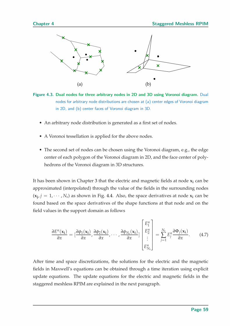
Chapter 4 Staggered Meshless RPIM
Figure 4.3. Dual nodes for three arbitrary nodes in 2D and 3D using Voronoi diagram. Dual
nodes for arbitrary node distributions are chosen at (a) center edges of Voronoi diagram
in 2D, and (b) center faces of Voronoi diagram in 3D.
• An arbitrary node distribution is generated as a first set of nodes.
• A Voronoi tessellation is applied for the above nodes.
• The second set of nodes can be chosen using the Voronoi diagram, e.g., the edge
center of each polygon of the Voronoi diagram in 2D, and the face center of poly-
hedrons of the Voronoi diagram in 3D structures.
It has been shown in Chapter 3 that the electric and magnetic fields at node xi can be
approximated (interpolated) through the value of the fields in the surrounding nodes
(xj, j = 1, · · · , Ns) as shown in Fig. 4.4. Also, the space derivatives at node xi can be
found based on the space derivatives of the shape functions at that node and on the
field values in the support domain as follows
∂En(xi)
∂x= [
∂φ1(xi)
∂x,
∂φ2(xi)
∂x, · · · ,
∂φNs(xi)
∂x]
En1
En2...
EnNs
=
Ns
∑j=1
Enj
∂Φj(xi)
∂x. (4.7)
After time and space discretizations, the solutions for the electric and the magnetic
fields in Maxwell’s equations can be obtained through a time iteration using explicit
update equations. The update equations for the electric and magnetic fields in the
staggered meshless RPIM are explained in the next paragraph.
Page 59
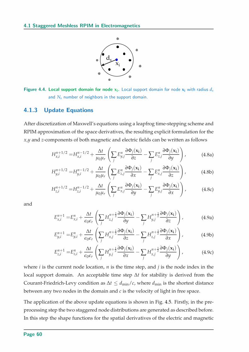
4.1 Staggered Meshless RPIM in Electromagnetics
Figure 4.4. Local support domain for node xi. Local support domain for node xi with radius ds
and Ns number of neighbors in the support domain.
4.1.3 Update Equations
After discretization of Maxwell’s equations using a leapfrog time-stepping scheme and
RPIM approximation of the space derivatives, the resulting explicit formulation for the
x,y and z-components of both magnetic and electric fields can be written as follows
Hn+1/2x,i =Hn−1/2
x,i +∆t
µ0µr
(
∑j
Eny,j
∂Φj(xi)
∂z−∑
j
Enz,j
∂Φj(xi)
∂y
), (4.8a)
Hn+1/2y,i =Hn−1/2
y,i +∆t
µ0µr
(
∑j
Enz,j
∂Φj(xi)
∂x−∑
j
Enx,j
∂Φj(xi)
∂z
), (4.8b)
Hn+1/2z,i =Hn−1/2
z,i +∆t
µ0µr
(
∑j
Enx,j
∂Φj(xi)
∂y−∑
j
Eny,j
∂Φj(xi)
∂x
), (4.8c)
and
En+1x,i =En
x,i +∆t
ǫ0ǫr
(
∑j
Hn+ 1
2z,j
∂Φj(xi)
∂y− ∑
j
Hn+ 1
2y,j
∂Φj(xi)
∂z
), (4.9a)
En+1y,i =En
y,i +∆t
ǫ0ǫr
(
∑j
Hn+ 1
2x,j
∂Φj(xi)
∂z− ∑
j
Hn+ 1
2z,j
∂Φj(xi)
∂x
), (4.9b)
En+1z,i =En
z,i +∆t
ǫ0ǫr
(
∑j
Hn+ 1
2y,j
∂Φj(xi)
∂x− ∑
j
Hn+ 1
2x,j
∂Φj(xi)
∂y
), (4.9c)
where i is the current node location, n is the time step, and j is the node index in the
local support domain. An acceptable time step ∆t for stability is derived from the
Courant-Friedrich-Levy condition as ∆t ≤ dmin/c, where dmin is the shortest distance
between any two nodes in the domain and c is the velocity of light in free space.
The application of the above update equations is shown in Fig. 4.5. Firstly, in the pre-
processing step the two staggered node distributions are generated as described before.
In this step the shape functions for the spatial derivatives of the electric and magnetic
Page 60
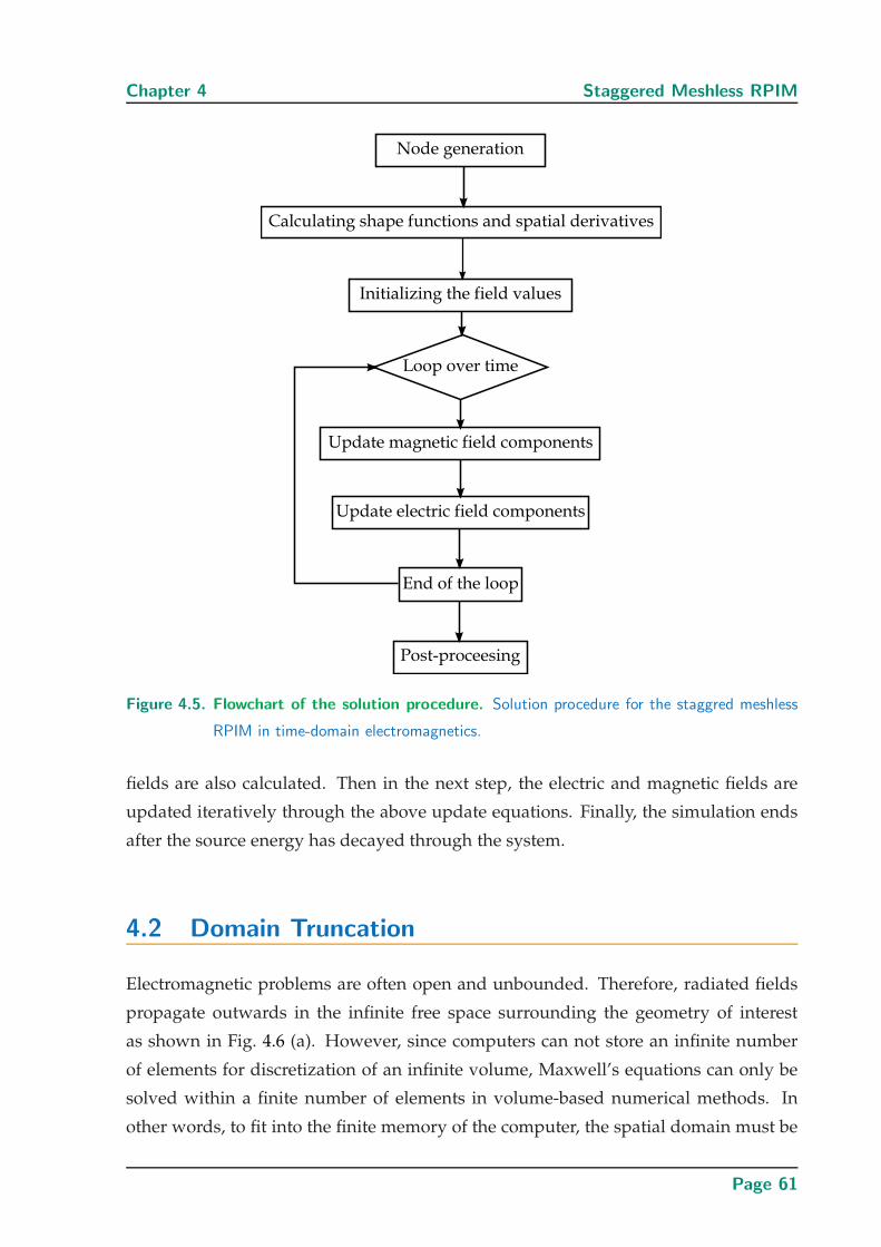
Chapter 4 Staggered Meshless RPIM
Figure 4.5. Flowchart of the solution procedure. Solution procedure for the staggred meshless
RPIM in time-domain electromagnetics.
fields are also calculated. Then in the next step, the electric and magnetic fields are
updated iteratively through the above update equations. Finally, the simulation ends
after the source energy has decayed through the system.
4.2 Domain Truncation
Electromagnetic problems are often open and unbounded. Therefore, radiated fields
propagate outwards in the infinite free space surrounding the geometry of interest
as shown in Fig. 4.6 (a). However, since computers can not store an infinite number
of elements for discretization of an infinite volume, Maxwell’s equations can only be
solved within a finite number of elements in volume-based numerical methods. In
other words, to fit into the finite memory of the computer, the spatial domain must be
Page 61
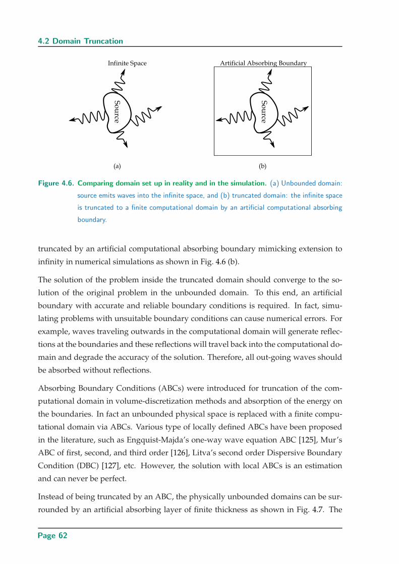
4.2 Domain Truncation
Figure 4.6. Comparing domain set up in reality and in the simulation. (a) Unbounded domain:
source emits waves into the infinite space, and (b) truncated domain: the infinite space
is truncated to a finite computational domain by an artificial computational absorbing
boundary.
truncated by an artificial computational absorbing boundary mimicking extension to
infinity in numerical simulations as shown in Fig. 4.6 (b).
The solution of the problem inside the truncated domain should converge to the so-
lution of the original problem in the unbounded domain. To this end, an artificial
boundary with accurate and reliable boundary conditions is required. In fact, simu-
lating problems with unsuitable boundary conditions can cause numerical errors. For
example, waves traveling outwards in the computational domain will generate reflec-
tions at the boundaries and these reflections will travel back into the computational do-
main and degrade the accuracy of the solution. Therefore, all out-going waves should
be absorbed without reflections.
Absorbing Boundary Conditions (ABCs) were introduced for truncation of the com-
putational domain in volume-discretization methods and absorption of the energy on
the boundaries. In fact an unbounded physical space is replaced with a finite compu-
tational domain via ABCs. Various type of locally defined ABCs have been proposed
in the literature, such as Engquist-Majda’s one-way wave equation ABC [125], Mur’s
ABC of first, second, and third order [126], Litva’s second order Dispersive Boundary
Condition (DBC) [127], etc. However, the solution with local ABCs is an estimation
and can never be perfect.
Instead of being truncated by an ABC, the physically unbounded domains can be sur-
rounded by an artificial absorbing layer of finite thickness as shown in Fig. 4.7. The
Page 62
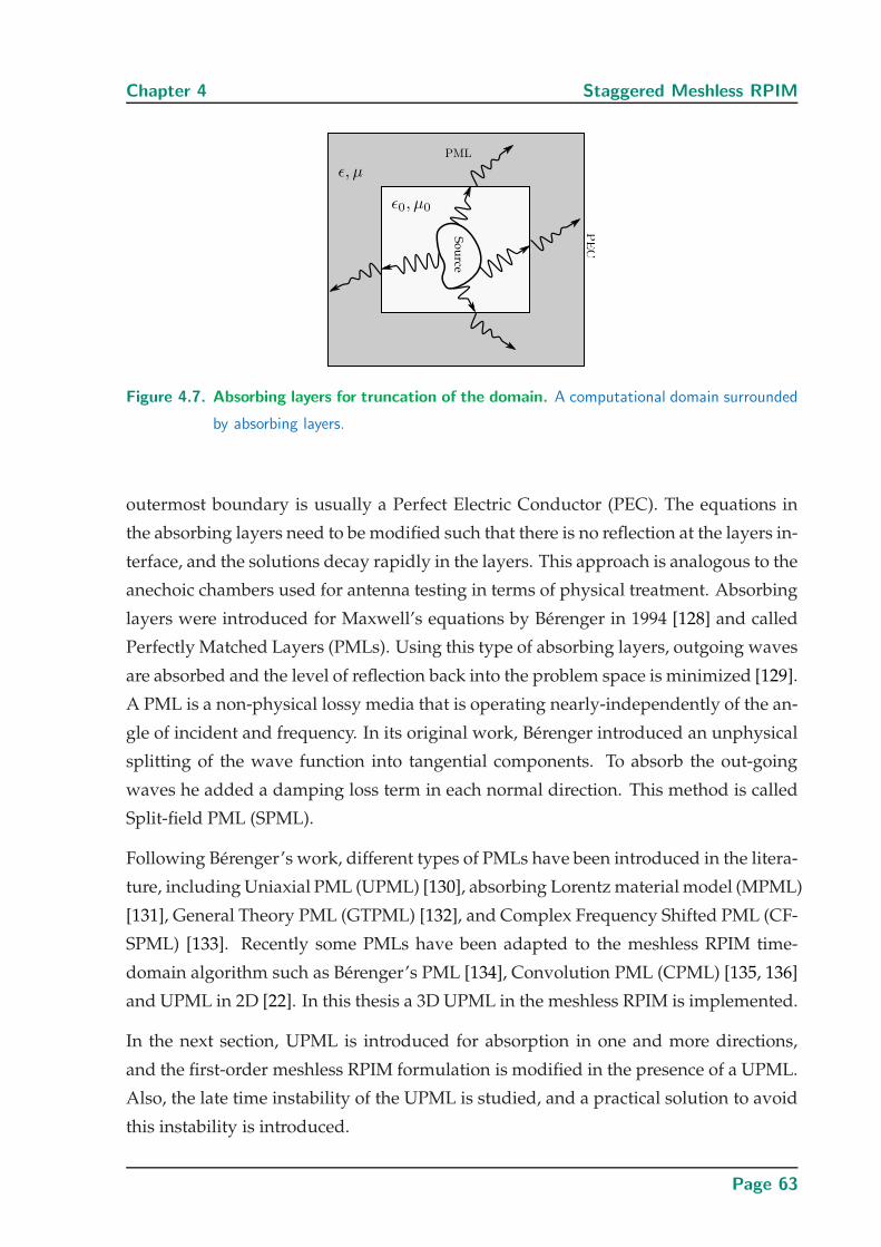
Chapter 4 Staggered Meshless RPIM
Figure 4.7. Absorbing layers for truncation of the domain. A computational domain surrounded
by absorbing layers.
outermost boundary is usually a Perfect Electric Conductor (PEC). The equations in
the absorbing layers need to be modified such that there is no reflection at the layers in-
terface, and the solutions decay rapidly in the layers. This approach is analogous to the
anechoic chambers used for antenna testing in terms of physical treatment. Absorbing
layers were introduced for Maxwell’s equations by Berenger in 1994 [128] and called
Perfectly Matched Layers (PMLs). Using this type of absorbing layers, outgoing waves
are absorbed and the level of reflection back into the problem space is minimized [129].
A PML is a non-physical lossy media that is operating nearly-independently of the an-
gle of incident and frequency. In its original work, Berenger introduced an unphysical
splitting of the wave function into tangential components. To absorb the out-going
waves he added a damping loss term in each normal direction. This method is called
Split-field PML (SPML).
Following Berenger’s work, different types of PMLs have been introduced in the litera-
ture, including Uniaxial PML (UPML) [130], absorbing Lorentz material model (MPML)
[131], General Theory PML (GTPML) [132], and Complex Frequency Shifted PML (CF-
SPML) [133]. Recently some PMLs have been adapted to the meshless RPIM time-
domain algorithm such as Berenger’s PML [134], Convolution PML (CPML) [135, 136]
and UPML in 2D [22]. In this thesis a 3D UPML in the meshless RPIM is implemented.
In the next section, UPML is introduced for absorption in one and more directions,
and the first-order meshless RPIM formulation is modified in the presence of a UPML.
Also, the late time instability of the UPML is studied, and a practical solution to avoid
this instability is introduced.
Page 63
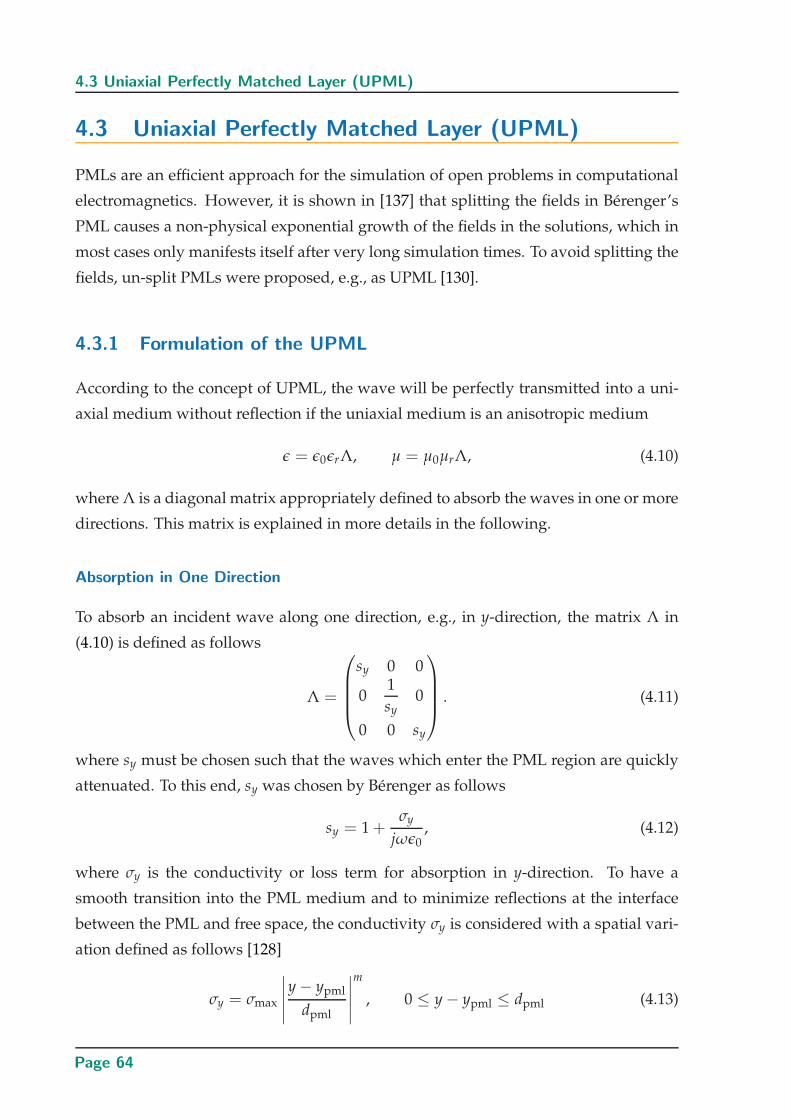
4.3 Uniaxial Perfectly Matched Layer (UPML)
4.3 Uniaxial Perfectly Matched Layer (UPML)
PMLs are an efficient approach for the simulation of open problems in computational
electromagnetics. However, it is shown in [137] that splitting the fields in Berenger’s
PML causes a non-physical exponential growth of the fields in the solutions, which in
most cases only manifests itself after very long simulation times. To avoid splitting the
fields, un-split PMLs were proposed, e.g., as UPML [130].
4.3.1 Formulation of the UPML
According to the concept of UPML, the wave will be perfectly transmitted into a uni-
axial medium without reflection if the uniaxial medium is an anisotropic medium
ǫ = ǫ0ǫrΛ, µ = µ0µrΛ, (4.10)
where Λ is a diagonal matrix appropriately defined to absorb the waves in one or more
directions. This matrix is explained in more details in the following.
Absorption in One Direction
To absorb an incident wave along one direction, e.g., in y-direction, the matrix Λ in
(4.10) is defined as follows
Λ =
sy 0 0
01
sy0
0 0 sy
. (4.11)
where sy must be chosen such that the waves which enter the PML region are quickly
attenuated. To this end, sy was chosen by Berenger as follows
sy = 1 +σy
jωǫ0, (4.12)
where σy is the conductivity or loss term for absorption in y-direction. To have a
smooth transition into the PML medium and to minimize reflections at the interface
between the PML and free space, the conductivity σy is considered with a spatial vari-
ation defined as follows [128]
σy = σmax
∣∣∣∣∣y − ypml
dpml
∣∣∣∣∣
m
, 0 ≤ y − ypml ≤ dpml (4.13)
Page 64
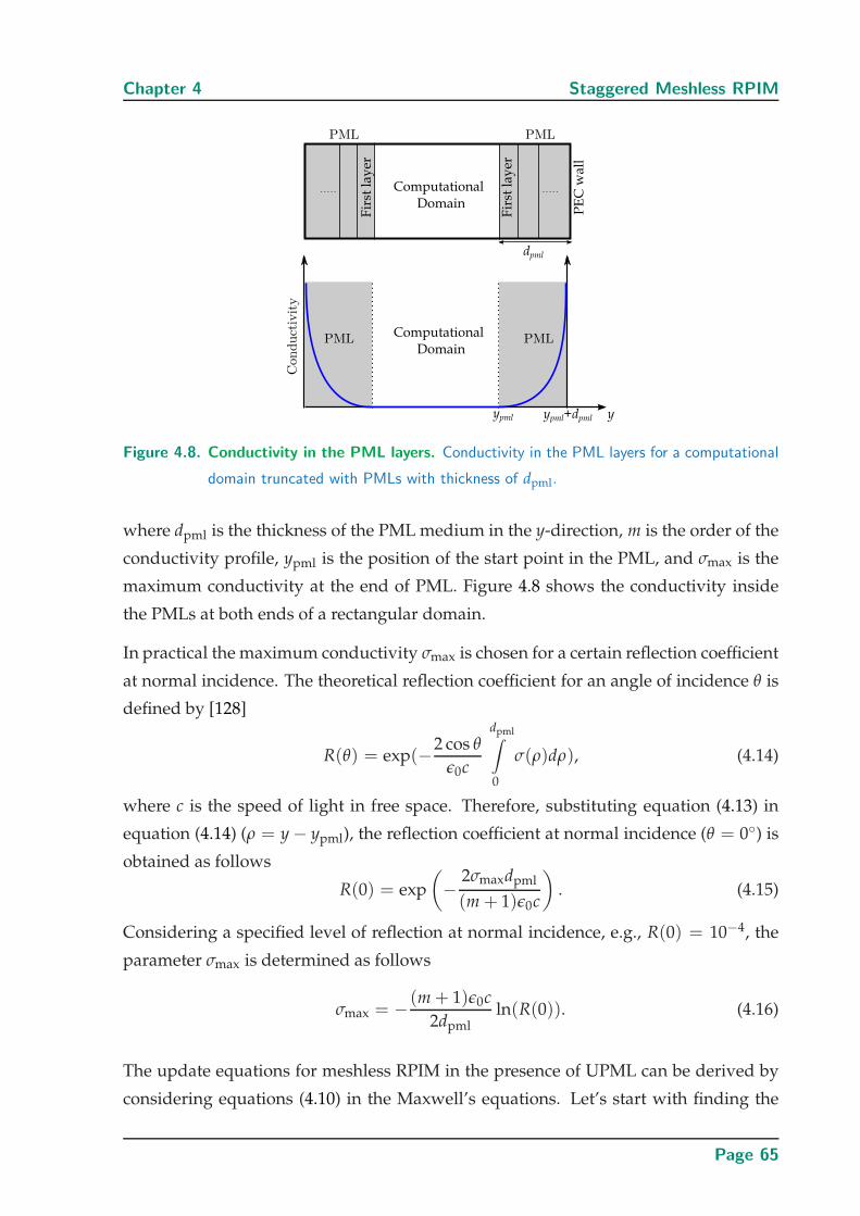
Chapter 4 Staggered Meshless RPIM
Figure 4.8. Conductivity in the PML layers. Conductivity in the PML layers for a computational
domain truncated with PMLs with thickness of dpml.
where dpml is the thickness of the PML medium in the y-direction, m is the order of the
conductivity profile, ypml is the position of the start point in the PML, and σmax is the
maximum conductivity at the end of PML. Figure 4.8 shows the conductivity inside
the PMLs at both ends of a rectangular domain.
In practical the maximum conductivity σmax is chosen for a certain reflection coefficient
at normal incidence. The theoretical reflection coefficient for an angle of incidence θ is
defined by [128]
R(θ) = exp(−2 cos θ
ǫ0c
dpml∫
0
σ(ρ)dρ), (4.14)
where c is the speed of light in free space. Therefore, substituting equation (4.13) in
equation (4.14) (ρ = y − ypml), the reflection coefficient at normal incidence (θ = 0) is
obtained as follows
R(0) = exp
(−
2σmaxdpml
(m + 1)ǫ0c
). (4.15)
Considering a specified level of reflection at normal incidence, e.g., R(0) = 10−4, the
parameter σmax is determined as follows
σmax = − (m + 1)ǫ0c
2dpmlln(R(0)). (4.16)
The update equations for meshless RPIM in the presence of UPML can be derived by
considering equations (4.10) in the Maxwell’s equations. Let’s start with finding the
Page 65
4.3 Uniaxial Perfectly Matched Layer (UPML)
update equations for all components of the electric field in 3D. The frequency-domain
version of Ampere’s law in the presence of UPML is expressed as follows
∇× H = jωǫ0ǫrΛE, (4.17)
which turns to the following equations by considering the curl operator and Λ as in
(4.11)
∂Hz
∂y− ∂Hy
∂z= jωǫ0ǫrsyEx, (4.18a)
∂Hx
∂z− ∂Hz
∂x= jωǫ0ǫr
1
syEy, (4.18b)
∂Hy
∂x− ∂Hx
∂y= jωǫ0ǫrsyEz. (4.18c)
By substituting the lossy anisotropy term in y-direction as sy = 1 + σy/(jωǫ0) in the
equation (4.18) (a), the following equation is obtained
∂Hz
∂y− ∂Hy
∂z= jωǫ0ǫr
(1 +
σy
jωǫ0
)Ex = jωǫ0ǫrEx + ǫrσyEx, (4.19)
which is equivalent to the following time-domain equation
1
ǫ0ǫr
(∂Hz
∂y− ∂Hy
∂z
)=
∂Ex
∂t+
σy
ǫ0Ex. (4.20)
Using RPIM to discretize the space derivatives, and using central finite differences to
discretize the time derivatives give
1
ǫ0ǫr
(
∑j
Hn+ 1
2z,j
∂φj(xi)
∂y− ∑
j
Hn+ 1
2y,j
∂φj(xi)
∂z
)=
En+1x − En
x
∆t+
σy
ǫ0
En+1x + En
x
2. (4.21)
After some simple manipulations the update equation for Ex is obtained as follows
En+1x,i = En
x,i
1 − σy∆t
2ǫ0
1 +σy∆t2ǫ0
+
∆t
ǫ0ǫr(1 +σy∆t2ǫ0
)(
∑j
Hn+ 1
2z,j
∂φj(xi)
∂y− ∑
j
Hn+ 1
2y,j
∂φj(xi)
∂z
).
(4.22)
In a very similar manner, the update equation for Ez can be determined as follows
En+1z,i = En
z,i
1 − σy∆t
2ǫ0
1 +σy∆t2ǫ0
+
∆t
ǫ0ǫr(1 +σy∆t2ǫ0
)(
∑j
Hn+ 1
2y,j
∂φj(xi)
∂x− ∑
j
Hn+ 1
2x,j
∂φj(xi)
∂y
).
(4.23)
Page 66
Chapter 4 Staggered Meshless RPIM
The update equation for the y-component of the electric field is obtained slightly differ-
ently, as follows: An auxiliary variable Dy is introduced to split the equation (4.18) (b)
into the two sub-equations [130]
1
ǫ0ǫr
(∂Hx
∂z− ∂Hz
∂x
)= jωDy, (4.24a)
Ey
1 +σy
jωǫ0
= Dy. (4.24b)
Converting the above equations to the time domain and then using space and time
discretizations result in the following update equations for the auxiliary variable Dy
and the electric field Ey
Dn+1y,i = Dn
y,i +∆t
ǫ0ǫr
(
∑j
Hn+ 1
2x,j
∂φj(xi)
∂z−∑
j
Hn+ 1
2z,j
∂φj(xi)
∂x
), (4.25a)
En+1y,i = En
y,i + Dn+1y,i (1 +
σy∆t
2ǫ0)− Dn
y,i(1 −σy∆t
2ǫ0), (4.25b)
where i is the current node location, n is the time step, and j is used for the node indices
in the local support domain.
The update equations for the magnetic field can be obtained same as the electric field.
Starting with Faraday’s law in the presence of UPML
∇× E = −jωµ0µrΛH, (4.26)
and substituting the curl operator and Λ, we obtain
∂Ey
∂z− ∂Ez
∂y= jωµ0µrsyHx, (4.27a)
∂Ez
∂x− ∂Ex
∂z= jωµ0µr
1
syHy, (4.27b)
∂Ex
∂y− ∂Ey
∂x= jωµ0µrsyHz. (4.27c)
Discretizing the (4.27) (a) and (c) is straightforward following the same procedure as
shown before. The update equations for Hx is then obtained as
Hn+ 1
2x,i = H
n− 12
x,i
1 − σy∆t
2ǫ0
1 +σy∆t2ǫ0
+
∆t
µ0µr(1 +σy∆t2ǫ0
)(
∑j
Eny,j
∂φj(xi)
∂z−∑
j
Enz,j
∂φj(xi)
∂y
),
(4.28)
Page 67
4.3 Uniaxial Perfectly Matched Layer (UPML)
and for Hz as
Hn+ 1
2z,i = H
n− 12
z,i
1 − σy∆t
2ǫ0
1 +σy∆t2ǫ0
+
∆t
µ0µr(1 +σy∆t2ǫ0
)(
∑j
Enx,j
∂φj(xi)
∂y− ∑
j
Eny,j
∂φj(xi)
∂x
).
(4.29)
To discretize (4.27) (b), an auxiliary variable By is introduced to split this expression
into the two following equations
1
µ0µr
(∂Ez
∂x− ∂Ex
∂z
)= jωBy, (4.30a)
Hy
1 +σy
jωǫ0
= By, (4.30b)
and finally the update equations for the auxiliary variable By and the magnetic field
Hy are obtained as follows
Bn+ 1
2y,i = B
n− 12
y,i +∆t
µ0µr
(
∑j
Enz,j
∂φj(xi)
∂x− ∑
j
Enx,j
∂φj(xi)
∂z
), (4.31a)
Hn+ 1
2y,i = H
n− 12
y,i + Bn+ 1
2y,i (1 +
σy∆t
2ǫ0)− B
n− 12
y,i (1 − σy∆t
2ǫ0). (4.31b)
These new update equations are a modification of the previous update equations in
(4.9) and (4.8) with introduction of UPML parameters in y-direction.
Absorption in Three Directions
To have absorption in three x, y and z-directions, the matrix Λ is defined as follows
Λ =
sysz
sx0 0
0sxsz
sy0
0 0sxsy
sz
. (4.32)
In this case, three auxiliary variables Dx, Dy and Dz are needed to split the three equa-
tions in the Ampere’s law as follows,
∂Hz
∂y− ∂Hy
∂z= jωszDx, Dx = ǫ0ǫr
sy
sxEx, (4.33a)
∂Hx
∂z− ∂Hz
∂x= jωsxDy, Dy = ǫ0ǫr
sz
syEy, (4.33b)
∂Hy
∂x− ∂Hx
∂y= jωsyDz, Dz = ǫ0ǫr
sx
szEz. (4.33c)
Page 68
Chapter 4 Staggered Meshless RPIM
Substituting sx, sy and sz in (4.33) (a) results in
∂Hz
∂y− ∂Hy
∂z= jωDx +
σz
ǫ0Dx, (4.34)
and
jωDx +σx
ǫ0Dx = ǫ0ǫr(jωEx +
σy
ǫ0Ex). (4.35)
Converting equations in (4.34) and (4.35) into the time domain, and using finite dif-
ferences to discretize time derivatives and RPIM to discretize space derivatives result
in(
∑j
Hn+ 1
2z,j
∂φj(xi)
∂y−∑
j
Hn+ 1
2y,j
∂φj(xi)
∂z
)=
Dn+1x − Dn−1
x
∆t+
σz
ǫ0
Dn+1x + Dn−1
x
2, (4.36)
Dn+1x − Dn−1
x
∆t+
σx
ǫ0
Dn+1x + Dn−1
x
2= ǫ0ǫr
(En+1
x − En−1x
∆t+
σy
ǫ0
En+1x + En−1
x
2
), (4.37)
which can be transformed into the following update equations for the auxiliary vari-
able Dx and the electric field Ex
Dn+1x = Dn−1
x
(1 − σz∆t
2ǫ0
1 + σz∆t2ǫ0
)+
∆t
1 + σz∆t2ǫ0
(
∑j
Hn+ 1
2z,j
∂φj(xi)
∂y−∑
j
Hn+ 1
2y,j
∂φj(xi)
∂z
), (4.38a)
En+1x = En−1
x
1 − σy∆t
2ǫ0
1 +σy∆t2ǫ0
+ Dn+1
x1
ǫ0ǫr
1 + σx∆t
2ǫ0
1 +σy∆t2ǫ0
− Dn−1
x1
ǫ0ǫr
1 − σx∆t
2ǫ0
1 +σy∆t2ǫ0
. (4.38b)
In a similar procedure the update equations for Dy and Ey can be obtained from (4.33) (b)
as follows
Dn+1y = Dn−1
y
(1 − σx∆t
2ǫ0
1 + σx∆t2ǫ0
)+
∆t
1 + σx∆t2ǫ0
(
∑j
Hn+ 1
2x,j
∂φj(xi)
∂z−∑
j
Hn+ 1
2z,j
∂φj(xi)
∂x
), (4.39a)
En+1y = En−1
y
(1 − σz∆t
2ǫ0
1 + σz∆t2ǫ0
)+ Dn+1
y1
ǫ0ǫr
1 +
σy∆t2ǫ0
1+ σz∆t2ǫ0
− Dn−1
y1
ǫ0ǫr
1 − σy∆t
2ǫ0
1 + σz∆t2ǫ0
. (4.39b)
Also, the update equations for the auxiliary variable Dz and the electric field Ez can be
found from (4.33) (c) as follows
Dn+1z = Dn−1
z
1 − σy∆t
2ǫ0
1 +σy∆t2ǫ0
+
∆t
1 +σy∆t2ǫ0
(
∑j
Hn+ 1
2y,j
∂φj(xi)
∂x− ∑
j
Hn+ 1
2x,j
∂φj(xi)
∂y
), (4.40a)
En+1z = En−1
z
(1 − σx∆t
2ǫ0
1 + σx∆t2ǫ0
)+ Dn+1
z1
ǫ0ǫr
(1 + σz∆t
2ǫ0
1 + σx∆t2ǫ0
)− Dn−1
z1
ǫ0ǫr
(1 − σz∆t
2ǫ0
1 + σx∆t2ǫ0
). (4.40b)
Page 69
4.3 Uniaxial Perfectly Matched Layer (UPML)
Now to find the update equations for the magnetic field components, matrix Λ is used
in Faraday’s law. Here again three auxiliary variables Bx, By, and Bz are required to
split the three equations in the Faraday’s law into the following equations
∂Ey
∂z− ∂Ez
∂y= jωsyBx, Bx = µ0µr
sz
sxHx, (4.41a)
∂Ez
∂x− ∂Ex
∂z= jωszBy, By = µ0µr
sx
syHy, (4.41b)
∂Ex
∂y− ∂Ey
∂x= jωsxBz, Bz = µ0µr
sy
szHz. (4.41c)
Again, substituting sx, sy and sz in the above equations, converting them to the time
domain, and finally discretizing space and time derivatives give the following update
equations for Bx and Hx
Bn+ 1
2x = B
n− 12
x
1 − σy∆t
2ǫ0
1 +σy∆t2ǫ0
+
∆t
1 +σy∆t2ǫ0
(
∑j
Eny,j
∂φj(xi)
∂z− ∑
j
Enz,j
∂φj(xi)
∂y
), (4.42a)
Hn+ 1
2x = H
n− 12
x
(1 − σz∆t
2ǫ0
1 + σz∆t2ǫ0
)+ B
n+ 12
x1
µ0µr
(1 + σx∆t
2ǫ0
1 + σz∆t2ǫ0
)− B
n− 12
x1
µ0µr
(1 − σx∆t
2ǫ0
1 + σz∆t2ǫ0
),
(4.42b)
and the update equations for the auxiliary variable By and the magnetic field Hy are as
follows
Bn+ 1
2y = B
n− 12
y
(1 − σz∆t
2ǫ0
1 + σz∆t2ǫ0
)+
∆t
1 + σz∆t2ǫ0
(
∑j
Enz,j
∂φj(xi)
∂x− ∑
j
Enx,j
∂φj(xi)
∂z
), (4.43a)
Hn+ 1
2y = H
n− 12
y
(1 − σx∆t
2ǫ0
1 + σx∆t2ǫ0
)+ B
n+ 12
y1
µ0µr
1 +
σy∆t2ǫ0
1 + σx∆t2ǫ0
− B
n− 12
y1
µ0µr
1 − σy∆t
2ǫ0
1 + σx∆t2ǫ0
.
(4.43b)
Also, the update equations for the auxiliary variable Bz and the magnetic field Hz can
be obtained as
Bn+ 1
2z = B
n− 12
z
(1 − σx∆t
2ǫ0
1 + σx∆t2ǫ0
)+
∆t
1 + σx∆t2ǫ0
(
∑j
Enx,j
∂φj(xi)
∂y− ∑
j
Eny,j
∂φj(xi)
∂x
), (4.44a)
Hn+ 1
2z = H
n− 12
z
1 − σy∆t
2ǫ0
1 +σy∆t2ǫ0
+ B
n+ 12
z1
µ0µr
1 + σz∆t
2ǫ0
1 +σy∆t2ǫ0
− B
n− 12
z1
µ0µr
1 − σz∆t
2ǫ0
1 +σy∆t2ǫ0
.
(4.44b)
Page 70
Chapter 4 Staggered Meshless RPIM
These update equations will be used later in the numerical examples where absorption
in all three directions is required. In these cases, UPMLs will be arranged to truncate
the computational domain in all directions.
4.3.2 Late-Time Instability in UPML
The existence of a late-time linear growth of the fields in the un-split PMLs was shown
in [138]. A small perturbation in the equations to avoid a singular coefficient matrix
was introduced as a remedy. This method successfully suppresses the late-time insta-
bility and the cost is a loss of the perfect matching condition at the air-PML interface.
In [139] it was shown that using CPML [133] results in stable solutions in the late time
and also the perfectly matched property is satisfied. However, it requires a larger nu-
merical effort and more memory compared to UPML.
In this section, we analyze the temporal behavior of the UPML in the meshless RPIM in
3D. To this end a rectangular waveguide with UPMLs at both sides is implemented as
test case. For the suppression of the late-time instability the method introduced in [138]
is modified for RPIM. It is shown that late-time instability can be significantly delayed
to later time by introducing of small losses inside the UPML after a sufficient decay of
the energy in the computational domain. This late introduction does not compromise
the accuracy of the solution as the perfect matching is retained in the initial simulation
phase.
Algorithm
Here, the late time instability of the UPML in y-direction is studied by considering
equation (4.24) in more detail. Transforming equation (4.24) to the time domain yields
∂Dy
∂t=
1
ǫ0ǫr
(∂Hx
∂z− ∂Hz
∂x
), (4.45a)
∂Ey
∂t=
∂Dy
∂t+
σy
ǫ0Dy. (4.45b)
After a long time, the fields in the absorbing layer are almost quiescent and the spatial
derivatives ∂/∂x, ∂/∂z are nearly zero. In the limit of lim∂x,∂z→0 the matrix form of
(4.45) is
∂
∂t
[Dy
Ey
]=
0 0σy
ǫ00
[
Dy
Ey
]. (4.46)
Page 71
4.3 Uniaxial Perfectly Matched Layer (UPML)
The coefficient matrix in (4.46) is singular with two zero eigenvalues. The solutions for
Dy and Ey are as follows
Dy = A1, (4.47a)
Ey =σy
ǫ0A1t, (4.47b)
where A1 is a constant. It can be clearly seen that the field values will increase with
time and the late-time solution is unbounded, i.e., will become unstable. To avoid
this singular coefficient matrix, two loss terms δ1/ǫ0Dy and δ2Ey can be introduced in
equation (4.45) as follows
∂Dy
∂t=
1
ǫ0ǫr
(∂Hx
∂z− ∂Hz
∂x
)− δ1
ǫ0Dy, (4.48a)
∂Ey
∂t=
∂Dy
∂t+
σy
ǫ0Dy−δ2Ey. (4.48b)
In this case and by considering the condition lim∂x,∂z→0 after a long time, the matrix
(4.46) is changed to the following
∂
∂t
[Dy
Ey
]=
− δ1
ǫ00
σy
ǫ0− δ1
ǫ0−δ2
[
Dy
Ey
], (4.49)
where both δ1, δ2 are small positive real values introduced to yield two eigenvalues
with negative real parts. The late-time solutions for (4.49) are as follows
Dy = A1exp
(− δ1
ǫ0t
), (4.50a)
Ey = B1exp
(− δ1
ǫ0t
)+ C1exp (−δ2t) , (4.50b)
where A1, B1 and C1 are constant. Since the new coefficient matrix in (4.49) has two
unequal eigenvalues (δ1/ǫ0, δ2), the late-time solutions, which are linearly increasing
with time, can be avoided.
The new update equations for the auxiliary variable Dy and the electric field Ey in the
presence of two loss terms are as follows
Dn+1y,i = Dn
y,i
(1 − δ1∆t
2ǫ0
1 + δ1∆t2ǫ0
)+
∆t
ǫ0ǫr(1 +δ1∆t2ǫ0
)
(
∑j
Hn+ 1
2x,j
∂φj(xi)
∂z− ∑
j
Hn+ 1
2z,j
∂φj(xi)
∂x
),
(4.51a)
En+1y,i = En
y,i
(1 − δ2∆t
2
1 + δ2∆t2
)+ Dn+1
y,i
1 +
σy∆t2ǫ0
1 + δ2∆t2
− Dn
y,i
1 − σy∆t
2ǫ0
1 + δ2∆t2
. (4.51b)
Page 72
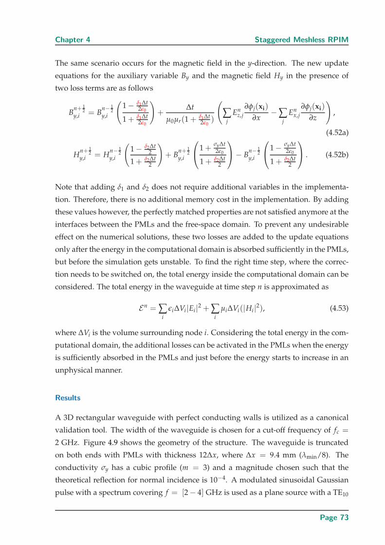
Chapter 4 Staggered Meshless RPIM
The same scenario occurs for the magnetic field in the y-direction. The new update
equations for the auxiliary variable By and the magnetic field Hy in the presence of
two loss terms are as follows
Bn+ 1
2y,i = B
n− 12
y,i
(1 − δ1∆t
2ǫ0
1 + δ1∆t2ǫ0
)+
∆t
µ0µr(1 +δ1∆t2ǫ0
)
(
∑j
Enz,j
∂φj(xi)
∂x− ∑
j
Enx,j
∂φj(xi)
∂z
),
(4.52a)
Hn+ 1
2y,i = H
n− 12
y,i
(1 − δ2∆t
2
1 + δ2∆t2
)+ B
n+ 12
y,i
1 +
σy∆t2ǫ0
1 + δ2∆t2
− B
n− 12
y,i
1 − σy∆t
2ǫ0
1 + δ2∆t2
. (4.52b)
Note that adding δ1 and δ2 does not require additional variables in the implementa-
tion. Therefore, there is no additional memory cost in the implementation. By adding
these values however, the perfectly matched properties are not satisfied anymore at the
interfaces between the PMLs and the free-space domain. To prevent any undesirable
effect on the numerical solutions, these two losses are added to the update equations
only after the energy in the computational domain is absorbed sufficiently in the PMLs,
but before the simulation gets unstable. To find the right time step, where the correc-
tion needs to be switched on, the total energy inside the computational domain can be
considered. The total energy in the waveguide at time step n is approximated as
En = ∑i
ǫi∆Vi|Ei|2 + ∑i
µi∆Vi(|Hi|2), (4.53)
where ∆Vi is the volume surrounding node i. Considering the total energy in the com-
putational domain, the additional losses can be activated in the PMLs when the energy
is sufficiently absorbed in the PMLs and just before the energy starts to increase in an
unphysical manner.
Results
A 3D rectangular waveguide with perfect conducting walls is utilized as a canonical
validation tool. The width of the waveguide is chosen for a cut-off frequency of fc =
2 GHz. Figure 4.9 shows the geometry of the structure. The waveguide is truncated
on both ends with PMLs with thickness 12∆x, where ∆x = 9.4 mm (λmin/8). The
conductivity σy has a cubic profile (m = 3) and a magnitude chosen such that the
theoretical reflection for normal incidence is 10−4. A modulated sinusoidal Gaussian
pulse with a spectrum covering f = [2 − 4] GHz is used as a plane source with a TE10
Page 73
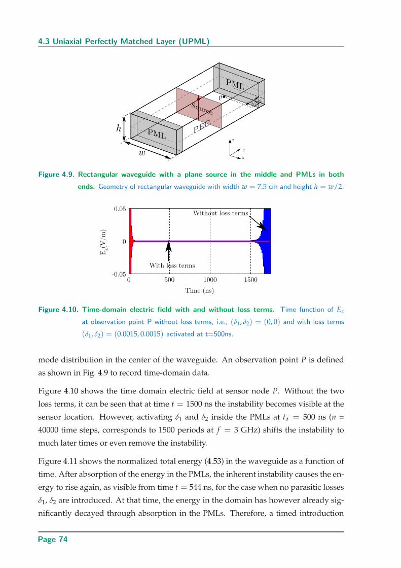
4.3 Uniaxial Perfectly Matched Layer (UPML)
Figure 4.9. Rectangular waveguide with a plane source in the middle and PMLs in both
ends. Geometry of rectangular waveguide with width w = 7.5 cm and height h = w/2.
Figure 4.10. Time-domain electric field with and without loss terms. Time function of Ez
at observation point P without loss terms, i.e., (δ1, δ2) = (0, 0) and with loss terms
(δ1, δ2) = (0.0015, 0.0015) activated at t=500ns.
mode distribution in the center of the waveguide. An observation point P is defined
as shown in Fig. 4.9 to record time-domain data.
Figure 4.10 shows the time domain electric field at sensor node P. Without the two
loss terms, it can be seen that at time t = 1500 ns the instability becomes visible at the
sensor location. However, activating δ1 and δ2 inside the PMLs at tδ = 500 ns (n =
40000 time steps, corresponds to 1500 periods at f = 3 GHz) shifts the instability to
much later times or even remove the instability.
Figure 4.11 shows the normalized total energy (4.53) in the waveguide as a function of
time. After absorption of the energy in the PMLs, the inherent instability causes the en-
ergy to rise again, as visible from time t = 544 ns, for the case when no parasitic losses
δ1, δ2 are introduced. At that time, the energy in the domain has however already sig-
nificantly decayed through absorption in the PMLs. Therefore, a timed introduction
Page 74
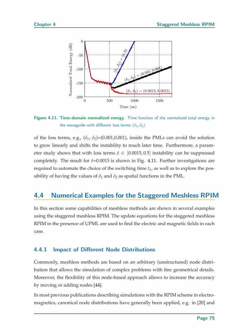
Chapter 4 Staggered Meshless RPIM
Figure 4.11. Time-domain normalized energy. Time function of the normalized total energy in
the waveguide with different loss terms (δ1, δ2).
of the loss terms, e.g., (δ1, δ2)=(0.001,0.001), inside the PMLs can avoid the solution
to grow linearly and shifts the instability to much later time. Furthermore, a param-
eter study shows that with loss terms δ ∈ [0.0015, 0.5] instability can be suppressed
completely. The result for δ=0.0015 is shown in Fig. 4.11. Further investigations are
required to automate the choice of the switching time tδ, as well as to explore the pos-
sibility of having the values of δ1 and δ2 as spatial functions in the PML.
4.4 Numerical Examples for the Staggered Meshless RPIM
In this section some capabilities of meshless methods are shown in several examples
using the staggered meshless RPIM. The update equations for the staggered meshless
RPIM in the presence of UPML are used to find the electric and magnetic fields in each
case.
4.4.1 Impact of Different Node Distributions
Commonly, meshless methods are based on an arbitrary (unstructured) node distri-
bution that allows the simulation of complex problems with fine geometrical details.
Moreover, the flexibility of this node-based approach allows to increase the accuracy
by moving or adding nodes [44].
In most previous publications describing simulations with the RPIM scheme in electro-
magnetics, canonical node distributions have generally been applied, e.g. in [20] and
Page 75
4.4 Numerical Examples for the Staggered Meshless RPIM
[22]. Here, the impact of non-ideal node distributions is considered, as this is a crucial
aspect for the robustness of the method. In a 3D waveguide example, a time-domain
simulation is performed for a regular node distribution and compared to the results
when the regular node distribution is randomly disturbed. A further comparison is
performed with a cylindrical node distribution that represents a case of a non-intuitive
distribution and can potentially introduce errors in the simulation. The results are ob-
tained in an otherwise identical setup.
Node Distribution
The spatial discretization of the RPIM scheme can be realized through arbitrarily placed
node distributions. As mentioned, for the solution of the first-order Maxwell’s equa-
tions, because of the coupling nature of electric and magnetic field components, two
separate sets of electric and magnetic field nodes (E- and H-nodes) are chosen to be
staggered in space. Similar to the FDTD method, this is best combined with a stag-
gered leapfrog time-stepping which results in second-order accuracy. Since meshless
methods are node based, complex geometries can be approximated by sophisticated
node distributions to conformally resolve the geometry. So far, the question of opti-
mal node distributions for a given geometry have only been partially answered, e.g.,
through node adaptivity. It can be generally assumed though that in complex geome-
tries, an initial node distribution will be based on the (known) geometry, but will not
be optimal in terms of the (unknown) electromagnetic field distribution. Hence, the
RPIM scheme is required to be robust for arbitrary node distributions.
In order to investigate the impact of non-ideal node placement, a test case of a rect-
angular waveguide is solved with different node distributions. The first strategy con-
siders a uniform node distribution: E-nodes are defined on a regular 3D grid. The
Voronoi algorithm [140] is then applied to the E-nodes, and H-nodes are placed in the
middle faces of each Voronoi cell. Figure 4.12 (a) shows a regular electric node distri-
bution with equal spacing of ∆x. Due to the rectangular geometry of the waveguide
structure with field components predominantly along the coordinate axes, this can be
considered as a ”good” node distribution. To test the effect of adding randomness
in the node distribution, i.e., by making the distribution of the nodes non-ideal, this
regular distribution is disturbed by introducing random node displacements. Random
displacements corresponding to a maximum of 5% and 10% of the grid period ∆x have
been generated, and an example is shown in Fig. 4.12 (b). As another example of a non-
ideal node arrangement, a cylindrical node distribution as shown in Fig. 4.12 (c) has
Page 76
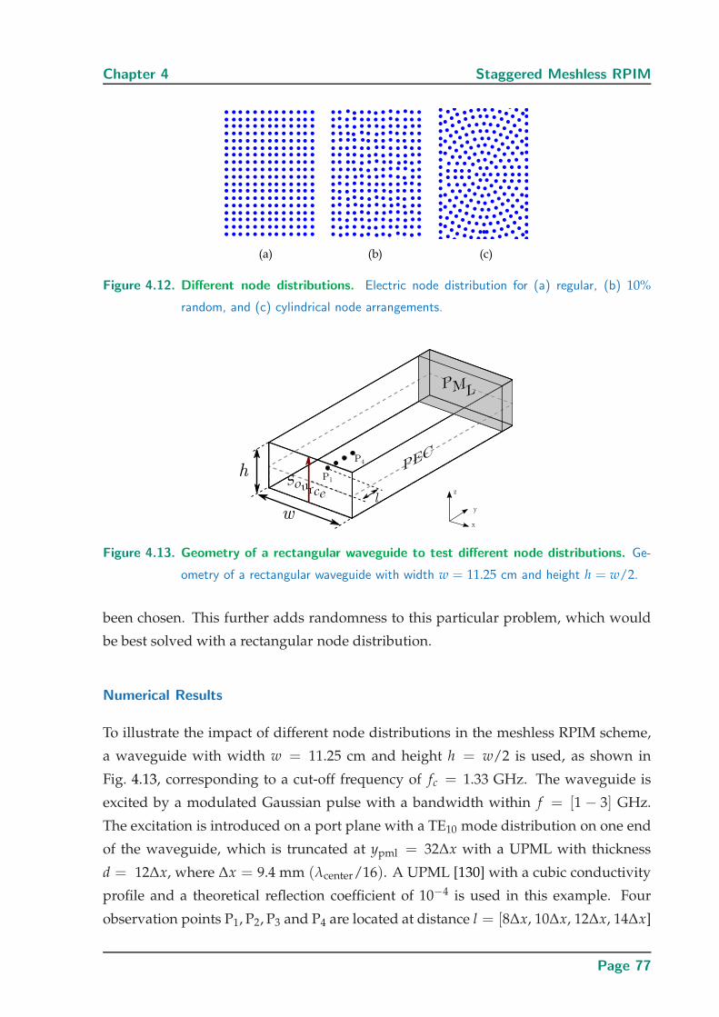
Chapter 4 Staggered Meshless RPIM
Figure 4.12. Different node distributions. Electric node distribution for (a) regular, (b) 10%
random, and (c) cylindrical node arrangements.
Figure 4.13. Geometry of a rectangular waveguide to test different node distributions. Ge-
ometry of a rectangular waveguide with width w = 11.25 cm and height h = w/2.
been chosen. This further adds randomness to this particular problem, which would
be best solved with a rectangular node distribution.
Numerical Results
To illustrate the impact of different node distributions in the meshless RPIM scheme,
a waveguide with width w = 11.25 cm and height h = w/2 is used, as shown in
Fig. 4.13, corresponding to a cut-off frequency of fc = 1.33 GHz. The waveguide is
excited by a modulated Gaussian pulse with a bandwidth within f = [1 − 3] GHz.
The excitation is introduced on a port plane with a TE10 mode distribution on one end
of the waveguide, which is truncated at ypml = 32∆x with a UPML with thickness
d = 12∆x, where ∆x = 9.4 mm (λcenter/16). A UPML [130] with a cubic conductivity
profile and a theoretical reflection coefficient of 10−4 is used in this example. Four
observation points P1, P2, P3 and P4 are located at distance l = [8∆x, 10∆x, 12∆x, 14∆x]
Page 77
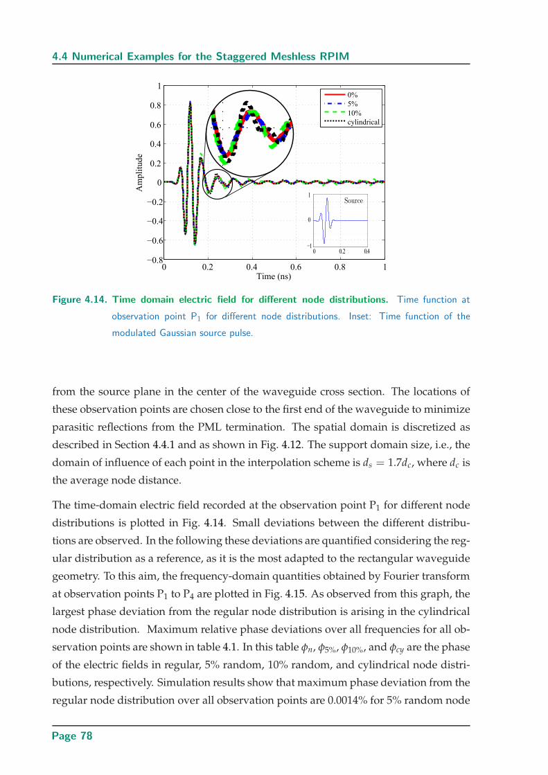
4.4 Numerical Examples for the Staggered Meshless RPIM
Figure 4.14. Time domain electric field for different node distributions. Time function at
observation point P1 for different node distributions. Inset: Time function of the
modulated Gaussian source pulse.
from the source plane in the center of the waveguide cross section. The locations of
these observation points are chosen close to the first end of the waveguide to minimize
parasitic reflections from the PML termination. The spatial domain is discretized as
described in Section 4.4.1 and as shown in Fig. 4.12. The support domain size, i.e., the
domain of influence of each point in the interpolation scheme is ds = 1.7dc, where dc is
the average node distance.
The time-domain electric field recorded at the observation point P1 for different node
distributions is plotted in Fig. 4.14. Small deviations between the different distribu-
tions are observed. In the following these deviations are quantified considering the reg-
ular distribution as a reference, as it is the most adapted to the rectangular waveguide
geometry. To this aim, the frequency-domain quantities obtained by Fourier transform
at observation points P1 to P4 are plotted in Fig. 4.15. As observed from this graph, the
largest phase deviation from the regular node distribution is arising in the cylindrical
node distribution. Maximum relative phase deviations over all frequencies for all ob-
servation points are shown in table 4.1. In this table φn, φ5%, φ10%, and φcy are the phase
of the electric fields in regular, 5% random, 10% random, and cylindrical node distri-
butions, respectively. Simulation results show that maximum phase deviation from the
regular node distribution over all observation points are 0.0014% for 5% random node
Page 78
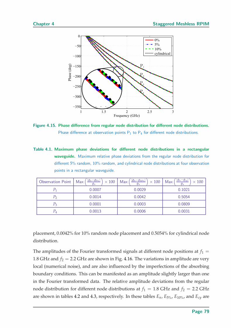
Chapter 4 Staggered Meshless RPIM
Figure 4.15. Phase difference from regular node distribution for different node distributions.
Phase difference at observation points P1 to P4 for different node distributions.
Table 4.1. Maximum phase deviations for different node distributions in a rectangular
waveguide. Maximum relative phase deviations from the regular node distribution for
different 5% random, 10% random, and cylindrical node distributions at four observation
points in a rectangular waveguide.
Observation Point Max(|φn−φ5%|
φn
)× 100 Max
(|φn−φ10%|
φn
)× 100 Max
( |φn−φcy|φn
)× 100
P1 0.0007 0.0029 0.1021
P2 0.0014 0.0042 0.5054
P3 0.0001 0.0003 0.0809
P4 0.0013 0.0006 0.0031
placement, 0.0042% for 10% random node placement and 0.5054% for cylindrical node
distribution.
The amplitudes of the Fourier transformed signals at different node positions at f1 =
1.8 GHz and f2 = 2.2 GHz are shown in Fig. 4.16. The variations in amplitude are very
local (numerical noise), and are also influenced by the imperfections of the absorbing
boundary conditions. This can be manifested as an amplitude slightly larger than one
in the Fourier transformed data. The relative amplitude deviations from the regular
node distribution for different node distributions at f1 = 1.8 GHz and f2 = 2.2 GHz
are shown in tables 4.2 and 4.3, respectively. In these tables En, E5%, E10%, and Ecy are
Page 79
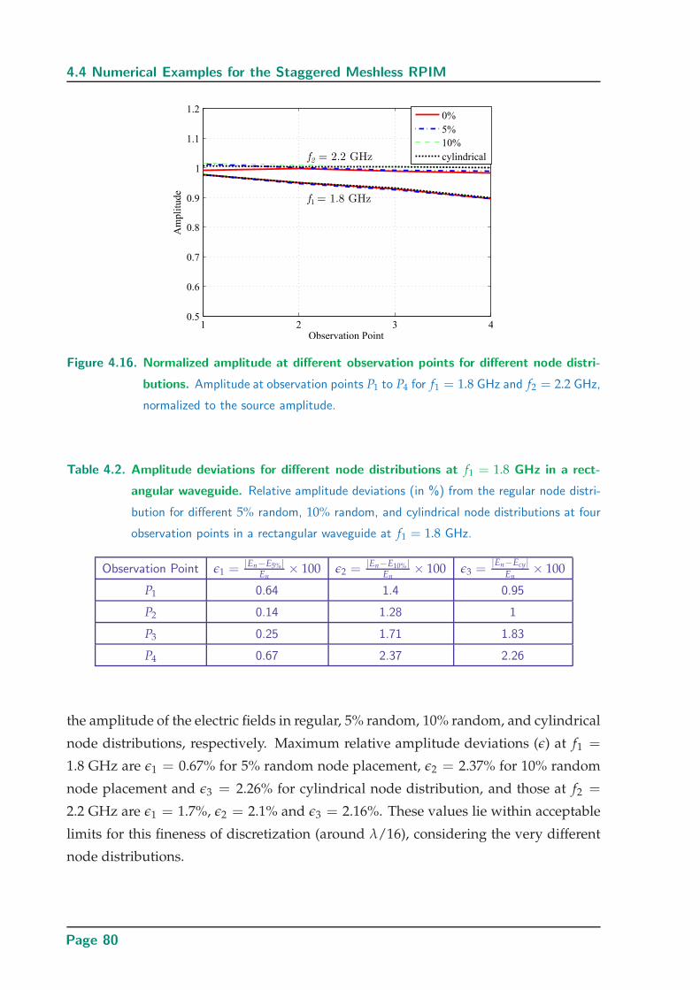
4.4 Numerical Examples for the Staggered Meshless RPIM
!
Figure 4.16. Normalized amplitude at different observation points for different node distri-
butions. Amplitude at observation points P1 to P4 for f1 = 1.8 GHz and f2 = 2.2 GHz,
normalized to the source amplitude.
Table 4.2. Amplitude deviations for different node distributions at f1 = 1.8 GHz in a rect-
angular waveguide. Relative amplitude deviations (in %) from the regular node distri-
bution for different 5% random, 10% random, and cylindrical node distributions at four
observation points in a rectangular waveguide at f1 = 1.8 GHz.
Observation Point ǫ1 = |En−E5%|En
× 100 ǫ2 = |En−E10%|En
× 100 ǫ3 =|En−Ecy|
En× 100
P1 0.64 1.4 0.95
P2 0.14 1.28 1
P3 0.25 1.71 1.83
P4 0.67 2.37 2.26
the amplitude of the electric fields in regular, 5% random, 10% random, and cylindrical
node distributions, respectively. Maximum relative amplitude deviations (ǫ) at f1 =
1.8 GHz are ǫ1 = 0.67% for 5% random node placement, ǫ2 = 2.37% for 10% random
node placement and ǫ3 = 2.26% for cylindrical node distribution, and those at f2 =
2.2 GHz are ǫ1 = 1.7%, ǫ2 = 2.1% and ǫ3 = 2.16%. These values lie within acceptable
limits for this fineness of discretization (around λ/16), considering the very different
node distributions.
Page 80
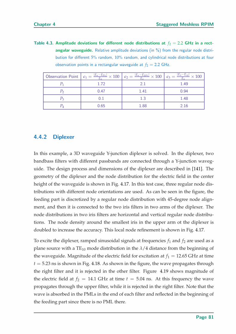
Chapter 4 Staggered Meshless RPIM
Table 4.3. Amplitude deviations for different node distributions at f2 = 2.2 GHz in a rect-
angular waveguide. Relative amplitude deviations (in %) from the regular node distri-
bution for different 5% random, 10% random, and cylindrical node distributions at four
observation points in a rectangular waveguide at f2 = 2.2 GHz.
Observation Point ǫ1 = |En−E5%|En
× 100 ǫ2 = |En−E10%|En
× 100 ǫ3 =|En−Ecy|
En× 100
P1 1.72 2.1 1.49
P2 0.47 1.41 0.94
P3 0.1 1.3 1.48
P4 0.65 1.88 2.16
4.4.2 Diplexer
In this example, a 3D waveguide Y-junction diplexer is solved. In the diplexer, two
bandbass filters with different passbands are connected through a Y-junction waveg-
uide. The design process and dimensions of the diplexer are described in [141]. The
geometry of the diplexer and the node distribution for the electric field in the center
height of the waveguide is shown in Fig. 4.17. In this test case, three regular node dis-
tributions with different node orientations are used. As can be seen in the figure, the
feeding part is discretized by a regular node distribution with 45-degree node align-
ment, and then it is connected to the two iris filters in two arms of the diplexer. The
node distributions in two iris filters are horizontal and vertical regular node distribu-
tions. The node density around the smallest iris in the upper arm ot the diplexer is
doubled to increase the accuracy. This local node refinement is shown in Fig. 4.17.
To excite the diplexer, ramped sinusoidal signals at frequencies f1 and f2 are used as a
plane source with a TE10 mode distribution in the λ/4 distance from the beginning of
the waveguide. Magnitude of the electric field for excitation at f1 = 12.65 GHz at time
t = 5.23 ns is shown in Fig. 4.18. As shown in the figure, the wave propagates through
the right filter and it is rejected in the other filter. Figure 4.19 shows magnitude of
the electric field at f2 = 14.1 GHz at time t = 5.04 ns. At this frequency the wave
propagates through the upper filter, while it is rejected in the right filter. Note that the
wave is absorbed in the PMLs in the end of each filter and reflected in the beginning of
the feeding part since there is no PML there.
Page 81
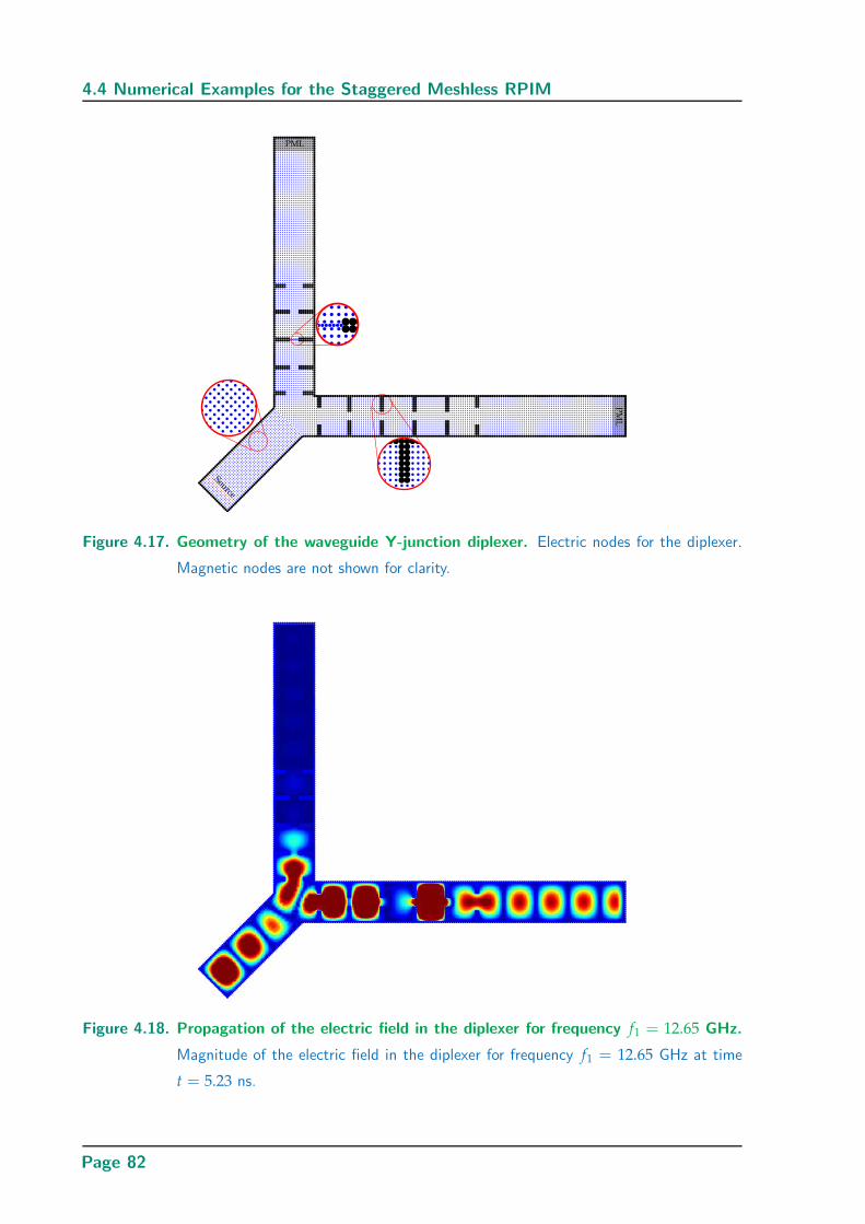
4.4 Numerical Examples for the Staggered Meshless RPIM
Figure 4.17. Geometry of the waveguide Y-junction diplexer. Electric nodes for the diplexer.
Magnetic nodes are not shown for clarity.
Figure 4.18. Propagation of the electric field in the diplexer for frequency f1 = 12.65 GHz.
Magnitude of the electric field in the diplexer for frequency f1 = 12.65 GHz at time
t = 5.23 ns.
Page 82
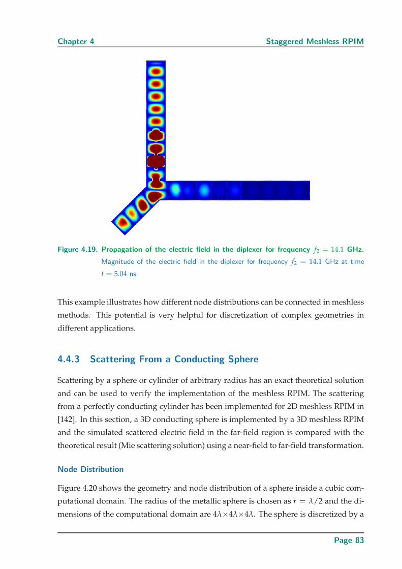
Chapter 4 Staggered Meshless RPIM
Figure 4.19. Propagation of the electric field in the diplexer for frequency f2 = 14.1 GHz.
Magnitude of the electric field in the diplexer for frequency f2 = 14.1 GHz at time
t = 5.04 ns.
This example illustrates how different node distributions can be connected in meshless
methods. This potential is very helpful for discretization of complex geometries in
different applications.
4.4.3 Scattering From a Conducting Sphere
Scattering by a sphere or cylinder of arbitrary radius has an exact theoretical solution
and can be used to verify the implementation of the meshless RPIM. The scattering
from a perfectly conducting cylinder has been implemented for 2D meshless RPIM in
[142]. In this section, a 3D conducting sphere is implemented by a 3D meshless RPIM
and the simulated scattered electric field in the far-field region is compared with the
theoretical result (Mie scattering solution) using a near-field to far-field transformation.
Node Distribution
Figure 4.20 shows the geometry and node distribution of a sphere inside a cubic com-
putational domain. The radius of the metallic sphere is chosen as r = λ/2 and the di-
mensions of the computational domain are 4λ×4λ×4λ. The sphere is discretized by a
Page 83
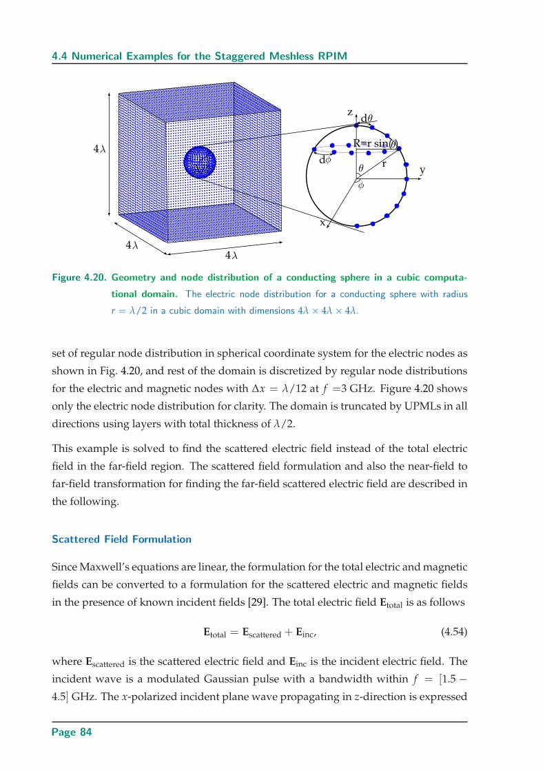
4.4 Numerical Examples for the Staggered Meshless RPIM
Figure 4.20. Geometry and node distribution of a conducting sphere in a cubic computa-
tional domain. The electric node distribution for a conducting sphere with radius
r = λ/2 in a cubic domain with dimensions 4λ × 4λ × 4λ.
set of regular node distribution in spherical coordinate system for the electric nodes as
shown in Fig. 4.20, and rest of the domain is discretized by regular node distributions
for the electric and magnetic nodes with ∆x = λ/12 at f =3 GHz. Figure 4.20 shows
only the electric node distribution for clarity. The domain is truncated by UPMLs in all
directions using layers with total thickness of λ/2.
This example is solved to find the scattered electric field instead of the total electric
field in the far-field region. The scattered field formulation and also the near-field to
far-field transformation for finding the far-field scattered electric field are described in
the following.
Scattered Field Formulation
Since Maxwell’s equations are linear, the formulation for the total electric and magnetic
fields can be converted to a formulation for the scattered electric and magnetic fields
in the presence of known incident fields [29]. The total electric field Etotal is as follows
Etotal = Escattered + Einc, (4.54)
where Escattered is the scattered electric field and Einc is the incident electric field. The
incident wave is a modulated Gaussian pulse with a bandwidth within f = [1.5 −4.5] GHz. The x-polarized incident plane wave propagating in z-direction is expressed
Page 84
Chapter 4 Staggered Meshless RPIM
as follows
Einc = exp
−(
t − (z−z0)c0
− 4σs√2σs
)2
sin
(2π f (t − (z − z0)
c0− 4σs)
), (4.55)
where σs determines the pulse width and z0 is a spatial offset. Since the incident electric
field is known in each point and each time step as shown in the equation (4.55), the
problem can be solved just for the unknown scattered electric field. To this end, the
scattered field formulation with its own boundary condition needs to be used. The
boundary condition for the total electric field on a conducting sphere is given by
Etotal,t = Escattered,t + Einc,t = 0, (4.56)
where subscript t shows the tangential component of the fields. From equation (4.56)
the following boundary condition for the scattered field on the conducting sphere can
be obtained
Escattered,t = −Einc,t. (4.57)
As a result, instead of solving the total electric field with condition Etotal,t = 0 on the
sphere, the problem can be solved for the scattered electric field with applying the
source on the sphere as a boundary condition as shown in equation (4.57). Note that
the solution for the total electric field can be determined by adding the incident field
to the scattered field solution in the post processing.
Near-Field to Far-Field Transformation
The far-field radiation pattern is one of the main characteristics that needs to be deter-
mined for a radiating object. The far-field region is typically assumed to be at distances
larger than 2D2/λ from the radiating object, where D is the dimension of the object and
λ is the wavelength. On the other hand, to save computational cost the computational
domain can not be extended to the far-field area. Therefore, usually the computational
domain is limited to the near-field region and a near-field to far-field transformation is
performed based on fields sampled on a closed Huygens’ surface around the object.
The near-field to far-field transformation is based on the equivalence theorem [143].
According to this theorem, if the tangential components of the fields are completely
known over a closed surface, the fields outside of that closed surface within the source-
free region can be determined.
Page 85
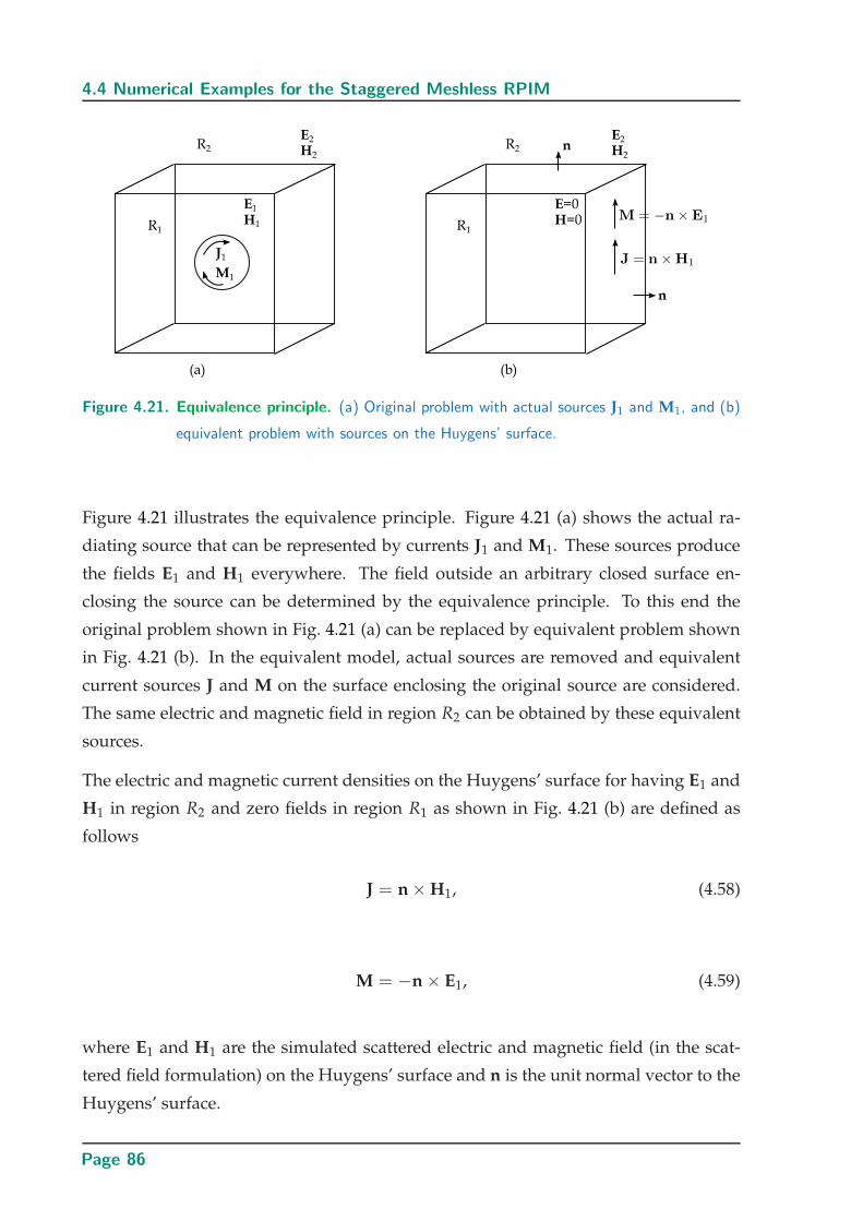
4.4 Numerical Examples for the Staggered Meshless RPIM
Figure 4.21. Equivalence principle. (a) Original problem with actual sources J1 and M1, and (b)
equivalent problem with sources on the Huygens’ surface.
Figure 4.21 illustrates the equivalence principle. Figure 4.21 (a) shows the actual ra-
diating source that can be represented by currents J1 and M1. These sources produce
the fields E1 and H1 everywhere. The field outside an arbitrary closed surface en-
closing the source can be determined by the equivalence principle. To this end the
original problem shown in Fig. 4.21 (a) can be replaced by equivalent problem shown
in Fig. 4.21 (b). In the equivalent model, actual sources are removed and equivalent
current sources J and M on the surface enclosing the original source are considered.
The same electric and magnetic field in region R2 can be obtained by these equivalent
sources.
The electric and magnetic current densities on the Huygens’ surface for having E1 and
H1 in region R2 and zero fields in region R1 as shown in Fig. 4.21 (b) are defined as
follows
J = n × H1, (4.58)
M = −n × E1, (4.59)
where E1 and H1 are the simulated scattered electric and magnetic field (in the scat-
tered field formulation) on the Huygens’ surface and n is the unit normal vector to the
Huygens’ surface.
Page 86
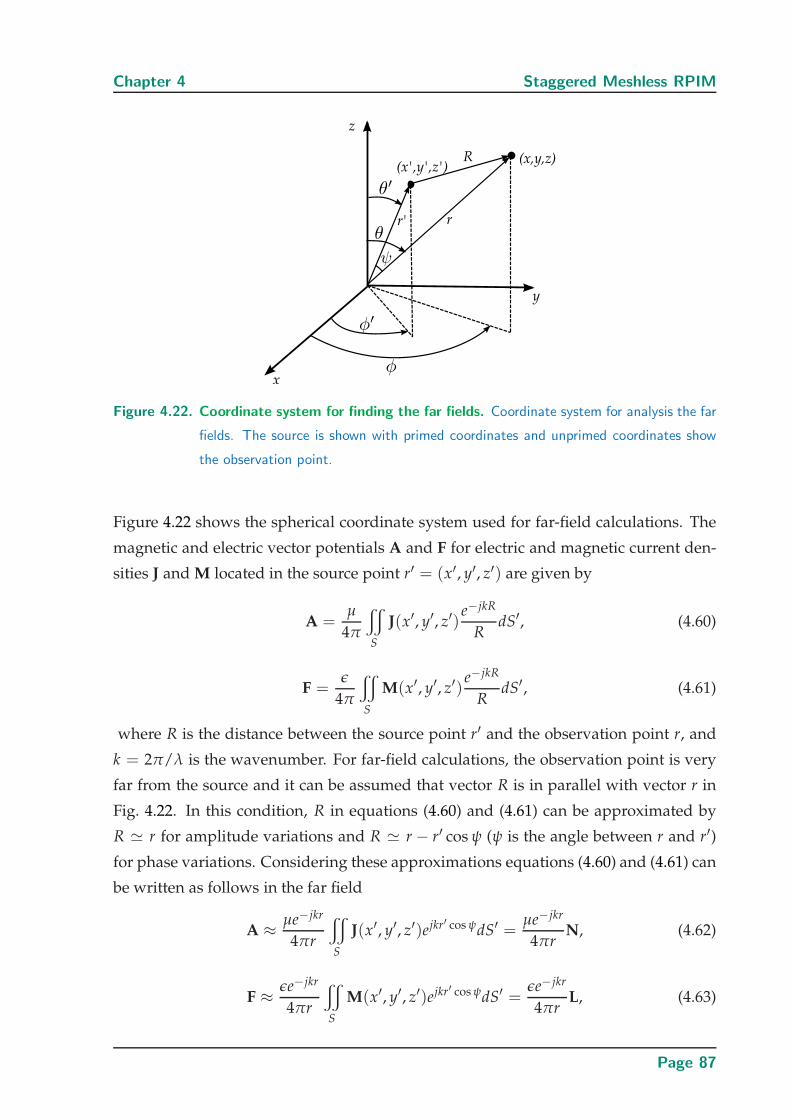
Chapter 4 Staggered Meshless RPIM
Figure 4.22. Coordinate system for finding the far fields. Coordinate system for analysis the far
fields. The source is shown with primed coordinates and unprimed coordinates show
the observation point.
Figure 4.22 shows the spherical coordinate system used for far-field calculations. The
magnetic and electric vector potentials A and F for electric and magnetic current den-
sities J and M located in the source point r′ = (x′, y′, z′) are given by
A =µ
4π
x
S
J(x′, y′, z′)e−jkR
RdS′, (4.60)
F =ǫ
4π
x
S
M(x′, y′, z′)e−jkR
RdS′, (4.61)
where R is the distance between the source point r′ and the observation point r, and
k = 2π/λ is the wavenumber. For far-field calculations, the observation point is very
far from the source and it can be assumed that vector R is in parallel with vector r in
Fig. 4.22. In this condition, R in equations (4.60) and (4.61) can be approximated by
R ≃ r for amplitude variations and R ≃ r − r′ cos ψ (ψ is the angle between r and r′)
for phase variations. Considering these approximations equations (4.60) and (4.61) can
be written as follows in the far field
A ≈ µe−jkr
4πr
x
S
J(x′, y′, z′)ejkr′ cos ψdS′ =µe−jkr
4πrN, (4.62)
F ≈ ǫe−jkr
4πr
x
S
M(x′, y′, z′)ejkr′ cos ψdS′ =ǫe−jkr
4πrL, (4.63)
Page 87
4.4 Numerical Examples for the Staggered Meshless RPIM
where N and L are as follows
N =x
S
J(x′, y′, z′)ejkr′ cos ψdS′, (4.64)
and
L =x
S
M(x′, y′, z′)ejkr′ cos ψdS′. (4.65)
Since spherical coordinates are more convenient for far-field calculations than the Carte-
sian coordinates, the following conversion matrix can be used to convert J(x′, y′, z′)
and M(x′, y′, z′) to spherical coordinates (r, θ, φ)
Jr
Jθ
Jφ
=
sin θ cos φ sin θ sin φ cos θ
cos θ cos φ cos θ sin φ − sin θ
− sin φ cos φ 0
Jx
Jy
Jz
. (4.66)
In this case, the integrals N and L in equations (4.64) and (4.65) in spherical coordinates
are written as
Nθ =x
s
Jθe+jkr′cos ψds
′=
x
s
[Jx cos θ cos φ + Jy cos θsinφ − Jzsinθ]e+jkr′
cos ψds′,
(4.67a)
Nφ =x
s
Jφe+jkr′cos ψds
′=
x
s
[−Jx sin φ + Jy cos φ]e+jkr′
cos ψds′, (4.67b)
and
Lθ =x
s
Mθe+jkr′
cos ψds′=
x
s
[Mx cos θ cos φ + My cos θ sin φ − Mz sin θ]e+jkr′
cos ψds′,
(4.68a)
Lφ =x
s
Mφe+jkr′cos ψds
′=
x
s
[−Mx sin φ + My cos φ]e+jkr′cos ψds
′. (4.68b)
Finally, the approximated electric field at the far field can be obtained as
Er ≃ 0, (4.69a)
Eθ ≃ − jke−jkr
4πr(Lφ + ηNθ), (4.69b)
Eφ ≃ +jke−jkr
4πr(Lθ − ηNφ), (4.69c)
Page 88
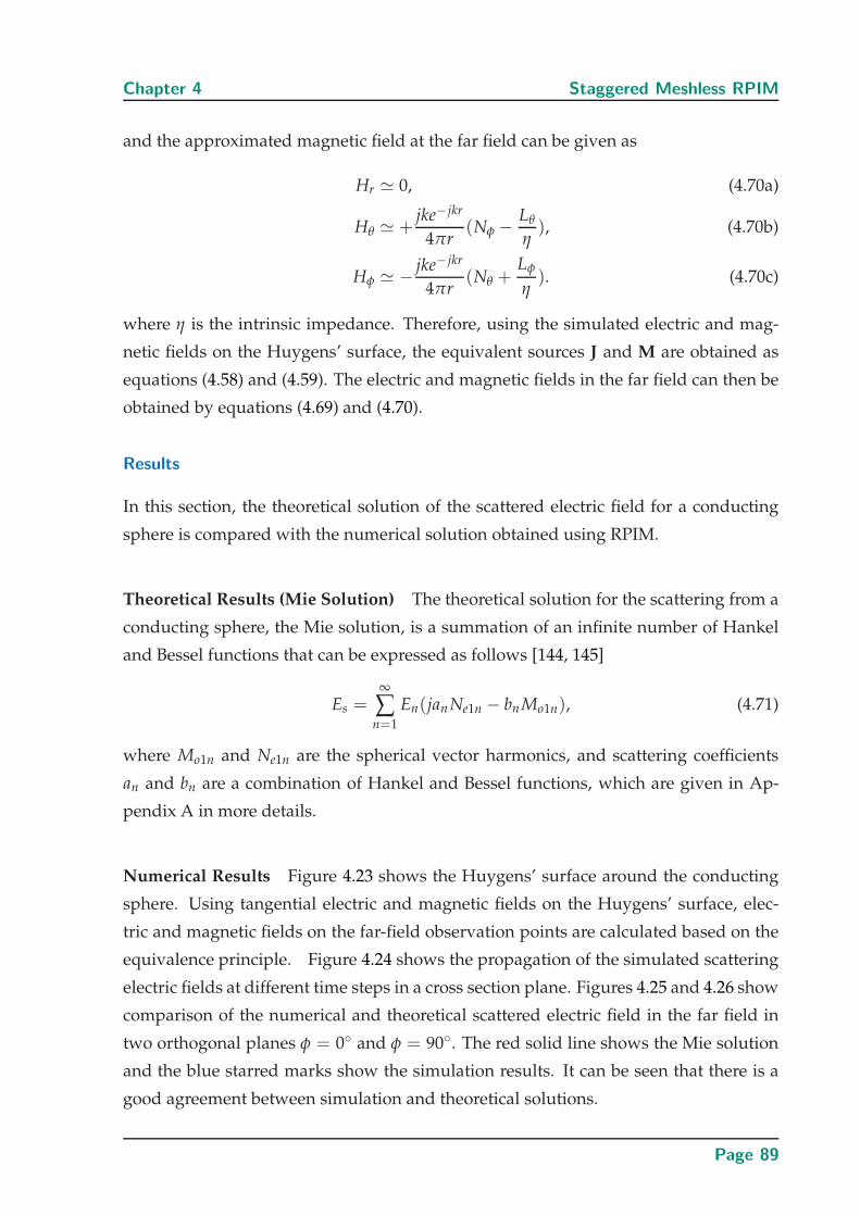
Chapter 4 Staggered Meshless RPIM
and the approximated magnetic field at the far field can be given as
Hr ≃ 0, (4.70a)
Hθ ≃ +jke−jkr
4πr(Nφ − Lθ
η), (4.70b)
Hφ ≃ − jke−jkr
4πr(Nθ +
Lφ
η). (4.70c)
where η is the intrinsic impedance. Therefore, using the simulated electric and mag-
netic fields on the Huygens’ surface, the equivalent sources J and M are obtained as
equations (4.58) and (4.59). The electric and magnetic fields in the far field can then be
obtained by equations (4.69) and (4.70).
Results
In this section, the theoretical solution of the scattered electric field for a conducting
sphere is compared with the numerical solution obtained using RPIM.
Theoretical Results (Mie Solution) The theoretical solution for the scattering from a
conducting sphere, the Mie solution, is a summation of an infinite number of Hankel
and Bessel functions that can be expressed as follows [144, 145]
Es =∞
∑n=1
En(jan Ne1n − bnMo1n), (4.71)
where Mo1n and Ne1n are the spherical vector harmonics, and scattering coefficients
an and bn are a combination of Hankel and Bessel functions, which are given in Ap-
pendix A in more details.
Numerical Results Figure 4.23 shows the Huygens’ surface around the conducting
sphere. Using tangential electric and magnetic fields on the Huygens’ surface, elec-
tric and magnetic fields on the far-field observation points are calculated based on the
equivalence principle. Figure 4.24 shows the propagation of the simulated scattering
electric fields at different time steps in a cross section plane. Figures 4.25 and 4.26 show
comparison of the numerical and theoretical scattered electric field in the far field in
two orthogonal planes φ = 0 and φ = 90. The red solid line shows the Mie solution
and the blue starred marks show the simulation results. It can be seen that there is a
good agreement between simulation and theoretical solutions.
Page 89
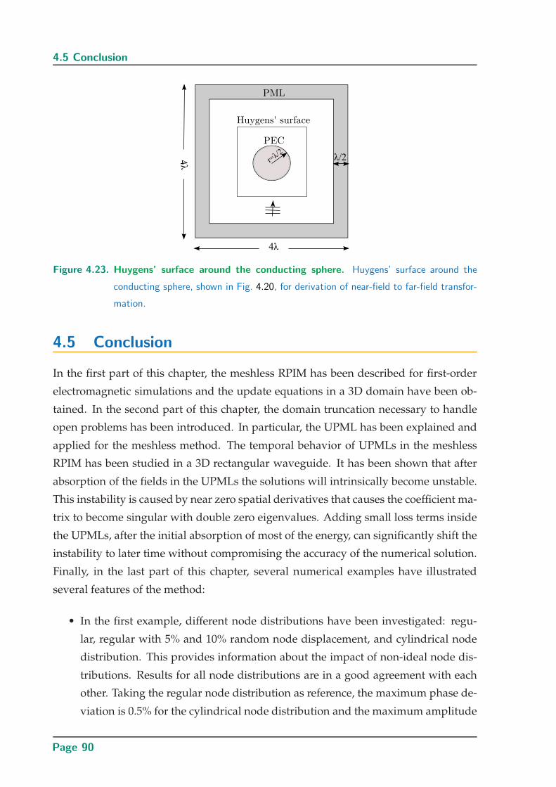
4.5 Conclusion
Figure 4.23. Huygens’ surface around the conducting sphere. Huygens’ surface around the
conducting sphere, shown in Fig. 4.20, for derivation of near-field to far-field transfor-
mation.
4.5 Conclusion
In the first part of this chapter, the meshless RPIM has been described for first-order
electromagnetic simulations and the update equations in a 3D domain have been ob-
tained. In the second part of this chapter, the domain truncation necessary to handle
open problems has been introduced. In particular, the UPML has been explained and
applied for the meshless method. The temporal behavior of UPMLs in the meshless
RPIM has been studied in a 3D rectangular waveguide. It has been shown that after
absorption of the fields in the UPMLs the solutions will intrinsically become unstable.
This instability is caused by near zero spatial derivatives that causes the coefficient ma-
trix to become singular with double zero eigenvalues. Adding small loss terms inside
the UPMLs, after the initial absorption of most of the energy, can significantly shift the
instability to later time without compromising the accuracy of the numerical solution.
Finally, in the last part of this chapter, several numerical examples have illustrated
several features of the method:
• In the first example, different node distributions have been investigated: regu-
lar, regular with 5% and 10% random node displacement, and cylindrical node
distribution. This provides information about the impact of non-ideal node dis-
tributions. Results for all node distributions are in a good agreement with each
other. Taking the regular node distribution as reference, the maximum phase de-
viation is 0.5% for the cylindrical node distribution and the maximum amplitude
Page 90
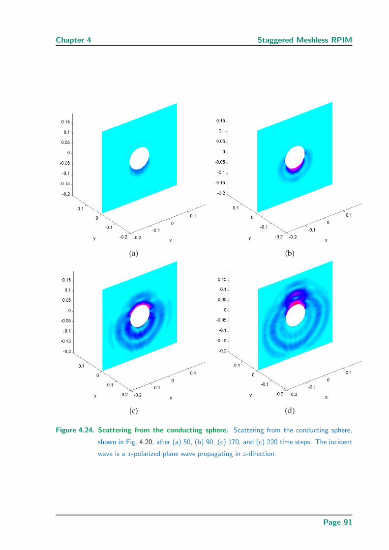
Chapter 4 Staggered Meshless RPIM
(a) (b)
(c) (d)
Figure 4.24. Scattering from the conducting sphere. Scattering from the conducting sphere,
shown in Fig. 4.20, after (a) 50, (b) 90, (c) 170, and (c) 220 time steps. The incident
wave is a x-polarized plane wave propagating in z-direction.
Page 91
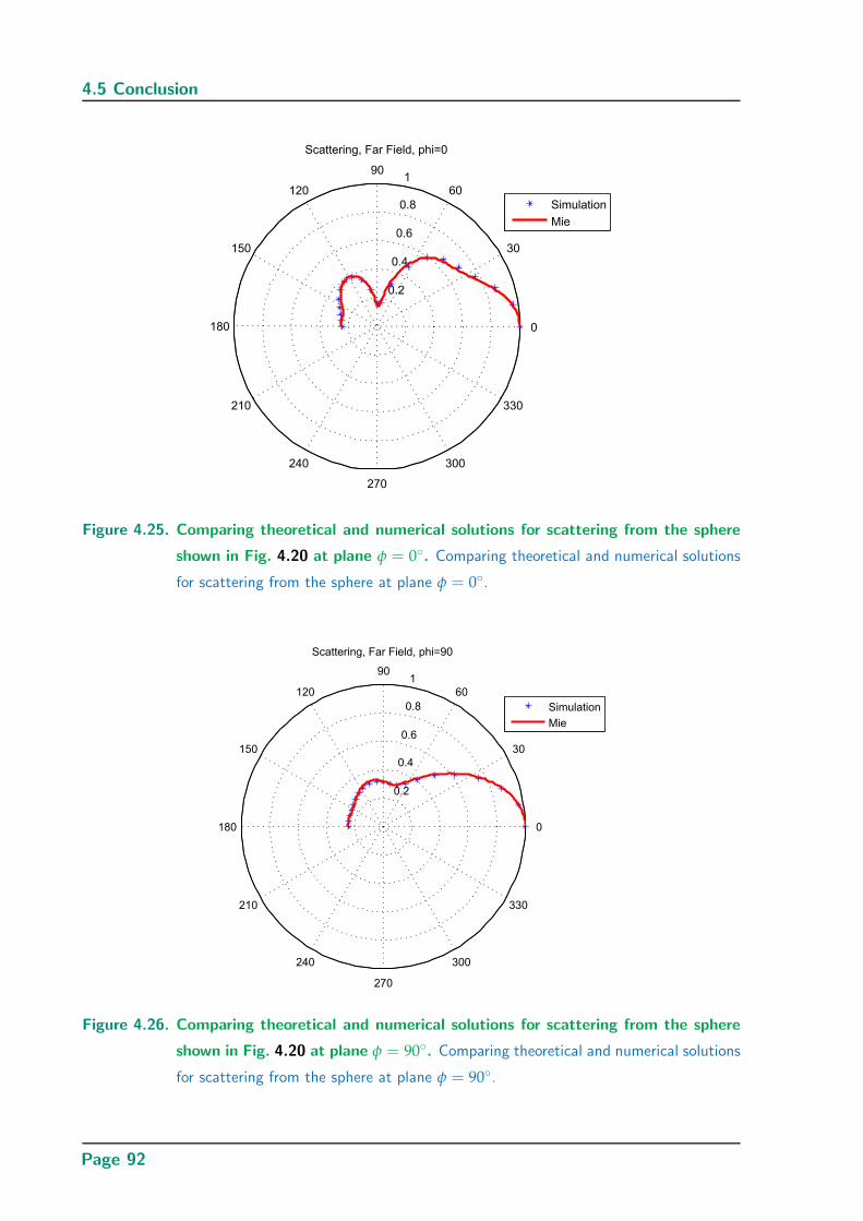
4.5 Conclusion
0.2
0.4
0.6
0.8
1
30
210
60
240
90
270
120
300
150
330
180 0
Scattering, Far Field, phi=0
Simulation
Mie
Figure 4.25. Comparing theoretical and numerical solutions for scattering from the sphere
shown in Fig. 4.20 at plane φ = 0. Comparing theoretical and numerical solutions
for scattering from the sphere at plane φ = 0.
0.2
0.4
0.6
0.8
1
30
210
60
240
90
270
120
300
150
330
180 0
Scattering, Far Field, phi=90
Simulation
Mie
Figure 4.26. Comparing theoretical and numerical solutions for scattering from the sphere
shown in Fig. 4.20 at plane φ = 90. Comparing theoretical and numerical solutions
for scattering from the sphere at plane φ = 90.
Page 92
Chapter 4 Staggered Meshless RPIM
deviation is 2.37% for 10% random node displacement. The results show that the
meshless RPIM scheme is robust for various node distributions, i.e., it yields very
close results for very different node arrangements. This increases confidence that
the method is suitable in versatile applications using complex geometries.
• In the second example, different parts of a diplexer have been discretized with
vertical, horizontal and a 45-degree oriented node distributions. The simulated
results show the wave propagation in the diplexer for two different frequencies.
This example shows the capability of meshless method to connect several do-
mains with various orientation of regular node distributions. This capability can
be useful in discretization of complex geometries.
• In the last example, the RPIM has been implemented to simulate scattering from
a perfect conducting sphere. A scattering formulation has been introduced and
the far-field scattered electric field has been obtained using a near-field to far-
field transformation. Finally, the far-field scattering simulation results have been
compared with the theoretical solutions. It has been shown that the simulation
results are in a good agreement with the theoretical results.
Page 93

Page 94
Chapter 5
Non-Staggered MeshlessRPIM: Vector Potential
Technique
IN the first part of this chapter a time-domain meshless algorithm
based on vector potentials is introduced for the analysis of tran-
sient electromagnetic fields. The proposed numerical algorithm is
a modification of the Radial Point Interpolation Method (RPIM), where ra-
dial basis functions are used for local interpolation of the vector potentials
and their derivatives. In the proposed implementation, solving the second-
order vector potential wave equation intrinsically enforces the divergence-
free property of the electric and magnetic fields. Furthermore, the compu-
tational effort associated with the generation of a dual node distribution (as
required for solving the first-order Maxwell’s equations) is avoided. In the
second part of this chapter an implementation of perfectly matched layer
for the magnetic vector potential method is proposed. In the final part of
this chapter, the proposed magnetic vector potential method is validated
with several examples of 2D waveguides and filters, and the convergence is
empirically demonstrated in terms of node density or size of local support
domains. It is further shown that inhomogeneous node distributions can
provide increased convergence rates, i.e., the same accuracy with smaller
number of nodes compared to a solution for homogeneous node distribu-
tion.
Page 95
5.1 Introduction
5.1 Introduction
A time-domain implementation of meshless Radial Point Interpolation Method (RPIM)
for the Maxwell’s equations was introduced in the previous chapter relying on stag-
gered node distributions for the electric and magnetic fields (Fig. 5.1 (a)). Such stag-
gered node arrangements have been proven to be robust in conjunction with most
time-domain numerical methods. However, in the framework of meshless methods,
the generation of an unstructured dual node distribution can be computationally costly
and restricts the freedom of node positions, which might reduce the potential advan-
tages of the scheme.
To overcome this challenge, a meshless vector potential technique is proposed in this
chapter to solve electromagnetic problems in a non-staggered node distribution as
shown in Fig. 5.1 (b). In this approach, on the one hand the order of the solved partial
differential equations is increased to second order, compared to the first-order Max-
well’s equations solved in the staggered meshless RPIM. On the other hand, since the
vector potentials are smoother functions of space than the field vectors near sources
and sharp discontinuities such as corners and edges, the numerical errors for a given
space discretization can be decreased [27]. Moreover, in this formalism, fields can be
described using three scalar wave equations, which has been shown in [27] to increase
the efficiency of a finite-difference time-domain solution and to save CPU time com-
pared to the classical staggered approach. Finally, and most importantly, the vector
potential technique preserves divergence property of the electric and magnetic fields
and thus prevents the appearance of spurious solutions [24, 25].
The vector potential technique was introduced to solve time-domain electromagnetic
fields with finite differences in [27, 146]. Various meshless implementations have been
later reported [147, 26, 148, 149]. In this chapter, we propose an efficient implementa-
tion of the time-domain meshless RPIM based on the local calculation of the magnetic
vector potential (A) in small support domains. The proposed method solves the wave
equation using Gaussian radial basis functions and a simplified explicit time integra-
tion, allowing for efficient high-accuracy simulations on small stencil sizes. This im-
plementation relies on the intrinsic capability of the RPIM method for accurate local
interpolations of higher-order derivatives, both in homogeneous and inhomogeneous
node distributions [150]. For simplicity, the method is firstly introduced in a 2D frame-
work. The convergence of the method is then validated using parallel plate waveguide
Page 96
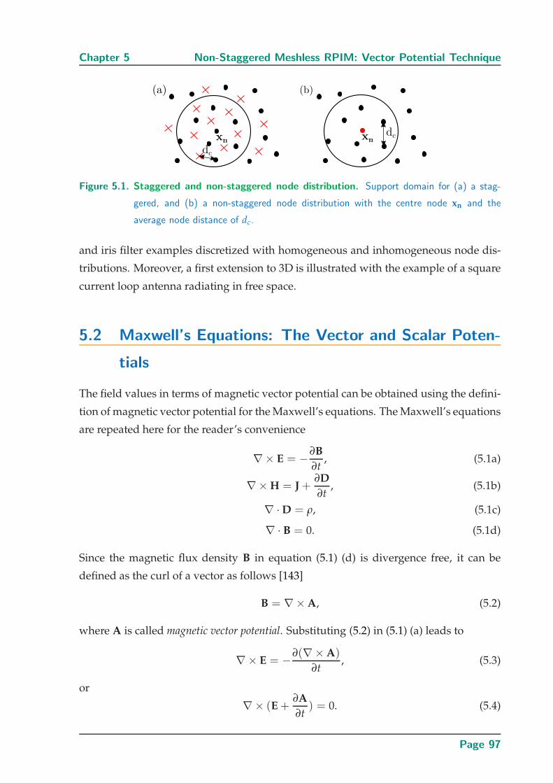
Chapter 5 Non-Staggered Meshless RPIM: Vector Potential Technique
Figure 5.1. Staggered and non-staggered node distribution. Support domain for (a) a stag-
gered, and (b) a non-staggered node distribution with the centre node xn and the
average node distance of dc.
and iris filter examples discretized with homogeneous and inhomogeneous node dis-
tributions. Moreover, a first extension to 3D is illustrated with the example of a square
current loop antenna radiating in free space.
5.2 Maxwell’s Equations: The Vector and Scalar Poten-
tials
The field values in terms of magnetic vector potential can be obtained using the defini-
tion of magnetic vector potential for the Maxwell’s equations. The Maxwell’s equations
are repeated here for the reader’s convenience
∇× E = −∂B
∂t, (5.1a)
∇× H = J +∂D
∂t, (5.1b)
∇ · D = ρ, (5.1c)
∇ · B = 0. (5.1d)
Since the magnetic flux density B in equation (5.1) (d) is divergence free, it can be
defined as the curl of a vector as follows [143]
B = ∇× A, (5.2)
where A is called magnetic vector potential. Substituting (5.2) in (5.1) (a) leads to
∇× E = −∂(∇× A)
∂t, (5.3)
or
∇× (E +∂A
∂t) = 0. (5.4)
Page 97
5.3 Magnetic Vector Potential
Since the curl of the vector in the parenthesis in (5.4) is equal to zero, this vector can be
expressed as the gradient of a scalar function V as follows
E +∂A
∂t= −∇V, (5.5)
where V is called electric scalar potential. From equation (5.5) the electric field can be
expressed as
E = −∂A
∂t−∇V. (5.6)
Substituting (5.2) and (5.6) in equation (5.1) (b) gives
∇× (1
µ∇× A) = J + ǫ
∂
∂t(−∂A
∂t−∇V), (5.7)
where using the identity ∇×∇× A = ∇(∇ · A)−∇2A and rearranging the terms in
equation (5.7) result in
∇2A − µǫ∂2A
∂t2−∇(∇ · A + µǫ
∂V
∂t) = −µJ. (5.8)
Finally, substituting (5.2) in (5.1) (c) gives
∇ · (∂A
∂t+∇V) = −ρ
ǫ, (5.9)
or
∇2V +∂
∂t(∇ · A) = −ρ
ǫ. (5.10)
Note that the definition of A in (5.2) automatically enforces the divergence-free prop-
erty of the magnetic flux density B. Therefore, equations (5.2), (5.6), (5.8), and (5.10)
are Maxwell’s equations in potential formulation.
5.3 Magnetic Vector Potential
Equations (5.2) and (5.6) do not uniquely define the potentials. In other words, if A
is changed to A′ = A +∇φ, the equation (5.2) is still satisfied since ∇× (∇φ) = 0.
However, the new A will change the E in (5.6) to − ∂A∂t −∇(V + ∂φ
∂t ). Therefore, if A
and V are simultaneously changed to A′ = A +∇φ and V ′ = V − ∂φ∂t , then both E
and B in (5.2) and (5.6) are consistently changed to satisfy Maxwell’s equations. Such
changes in A and V are called gauge transformation.
Page 98
Chapter 5 Non-Staggered Meshless RPIM: Vector Potential Technique
There are different gauges in the literature, e.g., the Lorenz gauge is written as
∇ · A = −µǫ∂V
∂t. (5.11)
Using this gauge the magnetic vector potential A and the electric scalar potential V in
(5.8) and (5.10) satisfy the inhomogeneous wave equations as
∇2A − µǫ∂2A
∂t2= −µJ, (5.12)
and
∇2V − µǫ∂2V
∂t2= −ρ
ǫ. (5.13)
The electric field can be calculated using (5.6) and (5.11) as
E = −∂A
∂t+
1
µǫ
∫∇(∇ · A)dt, (5.14)
and the magnetic field using (5.2) is
H =1
µ∇× A. (5.15)
From (5.12), it is seen that in the presence of a current source J, the magnetic vector
potential A satisfies the inhomogeneous wave equation. In this case instead of dis-
cretizing the domain for E and H and solving Maxwell’s equations using staggered
node distributions, a single set of nodes for A need only to be considered. Using the
Lorenz gauge condition, equation (5.12) is first solved and in a post-processing step, E
and H can be calculated through equations (5.14) and (5.15).
The vector potential technique automatically preserves the divergence property of the
electric field as well as of the magnetic field. From equation (5.14) the electric field can
be written in the frequency domain as follows
E = −jωA +1
jωµǫ∇(∇ · A). (5.16)
Taking the divergence of both sides of the above equation and multiplying by jωµǫ
result in
jωµǫ∇ · E = −µǫ(jω)2(∇ · A) +∇ ·∇(∇ · A) = −µǫ(jω)2(∇ · A) +∇2(∇ · A).
(5.17)
Using (5.12), the right hand side of the above equation can be rewritten to yield
jωµǫ∇ · E = −µ∇ · J, (5.18)
Page 99
5.4 Update Equations for A
or
jω(ǫ∇ · E) = −∇ · J. (5.19)
It can be concluded that in the source-free region (J = 0), ∇ · E is a constant in time.
Considering zero initial values for the electric field E in a time-domain solver it can be
concluded that the electric field is divergence free in the source-free region.
It is worth mentioning that in the presence of magnetic sources, the electric vector
potential F needs to be solved [143]. Note that this could be made in parallel to the A,
and on the same node distribution. Finally the total electric and magnetic fields can be
calculated by superposition of the fields obtained by A and F.
5.4 Update Equations for A
Using the RPIM algorithm to discretize space derivatives and finite differences to dis-
cretize time derivatives in (5.12) lead to a discretized expression for the magnetic vector
potential. In the non-staggered meshless RPIM the boundary conditions are related to
the derivative of the fields. Therefore, a local coordinate system is required to imple-
ment accurate derivative boundary conditions. The update equations for the magnetic
vector potential in Cartesian coordinate system is first introduced. To handle curved
boundaries, the update equations for the magnetic vector potential in polar coordinate
system is then introduced, which will be used for the PEC curved boundary nodes in
the next section.
5.4.1 Cartesian Coordinates
The explicit update equations for the magnetic vector potential can be obtained in
Cartesian coordinates by discretization of (5.12) through RPIM and finite difference
methods. In a 2D TEz framework, i.e., with the magnetic vector potential and con-
sequently the electric field perpendicular to the xy-plane and constant in z-direction,
the update equation for the z-component of the magnetic vector potential at location
x = (x, y) is derived as
An+1z = 2An
z − An−1z +
(∆t)2
µǫ
(∂2φ(x)
∂x2An
z +∂2φ(x)
∂y2An
z
)+
(∆t)2
ǫJnz . (5.20)
Expanding to 3D Cartesian coordinates, the Laplacian operator is given as
∇2A = (∇2Ax,∇2Ay,∇2Az), (5.21)
Page 100
Chapter 5 Non-Staggered Meshless RPIM: Vector Potential Technique
and the update equations for different components of the magnetic vector potential
can be obtained separately in a similar way starting from (5.12).
5.4.2 Polar Coordinates
The polar coordinate system with components denoted as (ρ, Φ) can be used as a local
coordinate system to increase the accuracy of simulations for curved boundaries. In
order to write the vector Laplacian operator in the polar coordinates, it is best to start
from the equivalent expression
∇2A = ∇(∇ · A)−∇× (∇× A). (5.22)
Using the curl and divergence in the polar coordinate system, as explicitly given in
Appendix B, and after some manipulations, the following expression is obtained for
the Laplacian operator
∇2A = (∇2Aρ −Aρ
ρ2− 2
ρ2
∂AΦ
∂Φ)ρ + (∇2AΦ − AΦ
ρ2+
2
ρ2
∂Aρ
∂Φ)Φ, (5.23)
where
∇2Aρ =1
ρ
∂
ρ(ρ
∂(Aρ)
∂ρ) +
1
ρ2
∂2Aρ
∂Φ2, (5.24)
and
∇2Aφ =1
ρ
∂
ρ(ρ
∂(Aφ)
∂ρ) +
1
ρ2
∂2Aφ
∂Φ2. (5.25)
Using the expression (5.23) in (5.12), each component of A in the polar coordinate sys-
tem satisfies the wave equation for the magnetic vector potential as follows
(∇2A)ρ − µǫ∂2 Aρ
∂t2= −µJρ, (5.26)
and
(∇2A)φ − µǫ∂2 Aφ
∂t2= −µJφ. (5.27)
The update equations for each component of the magnetic vector potential in the po-
lar coordinate system can be obtained by discretizing these two equations. However,
since the polar coordinate system is only used for the curved boundary nodes in this
thesis, the update equations for boundary nodes can be simplified using the boundary
conditions as shown in the next section.
Page 101
5.5 Perfect Electric Boundary Conditions for A
5.5 Perfect Electric Boundary Conditions for A
Boundary conditions for the magnetic vector potential can be adapted from boundary
conditions for the electric or magnetic fields in the Maxwell’s equations.
Perfect electric boundary conditions for the magnetic vector potential in Cartesian and
polar coordinate systems are introduced in the following.
5.5.1 Cartesian Coordinates
Boundary conditions for the Perfect Electric Conductor (PEC) in the magnetic vector
potential method can be obtained by enforcing the tangential component of the electric
field to zero (Eτ = 0) in (5.14). These boundary conditions can be derived as follows
[27]
Aτ = 0,∂An
∂n= 0, (5.28)
where n indicates the component normal to the boundary, Aτ and An are the tangential
and the normal components of A, respectively.
5.5.2 Polar Coordinates
As mentioned before, a polar coordinate system can be used as a local coordinate sys-
tem to handle curved boundaries. Generally, an arbitrary curved boundary can be
approximated by connecting different arcs of various circles. For simplicity an arc of a
circle centered at the origin is considered here. In this case, perfect electric boundary
conditions for the magnetic vector potential in the polar coordinate system can be ob-
tained by enforcing EΦ = 0 in (5.14). In this coordinate system, the term ∇(∇ · A) in
(5.14) becomes
∇(∇ · A) =∂
∂ρ(
Aρ
ρ+
∂Aρ
∂ρ+
1
ρ
∂AΦ
∂Φ)ρ +
1
ρ
∂
∂Φ(
Aρ
ρ+
∂Aρ
∂ρ+
1
ρ
∂AΦ
∂Φ)Φ. (5.29)
The identities to find this expression are given in Appendix B. Imposing the condition
EΦ = 0 in (5.14) leads to
EΦ = −∂AΦ
∂t+
1
µǫ
∫1
ρ
∂
∂Φ(
Aρ
ρ+
∂Aρ
∂ρ+
1
ρ
∂AΦ
∂Φ)dt = 0. (5.30)
Considering that each term of the sum in (5.30) must be equal to zero results in the
following conditions
AΦ = 0, (5.31)
Page 102
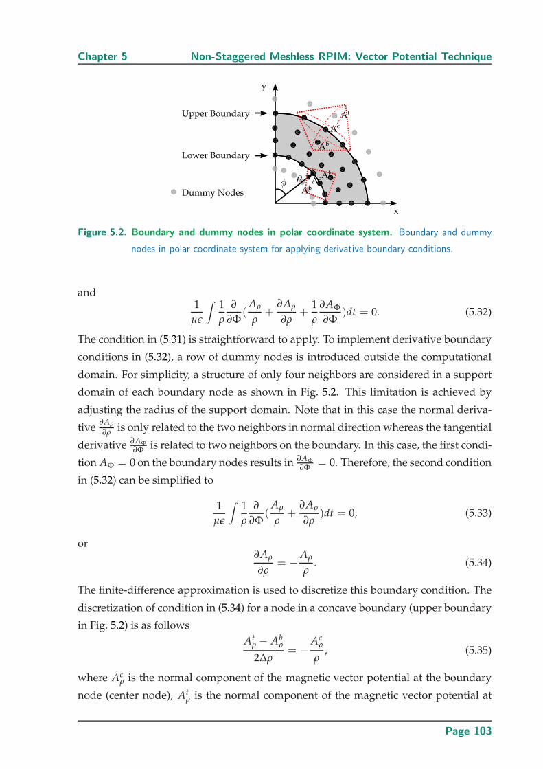
Chapter 5 Non-Staggered Meshless RPIM: Vector Potential Technique
Figure 5.2. Boundary and dummy nodes in polar coordinate system. Boundary and dummy
nodes in polar coordinate system for applying derivative boundary conditions.
and1
µǫ
∫1
ρ
∂
∂Φ(
Aρ
ρ+
∂Aρ
∂ρ+
1
ρ
∂AΦ
∂Φ)dt = 0. (5.32)
The condition in (5.31) is straightforward to apply. To implement derivative boundary
conditions in (5.32), a row of dummy nodes is introduced outside the computational
domain. For simplicity, a structure of only four neighbors are considered in a support
domain of each boundary node as shown in Fig. 5.2. This limitation is achieved by
adjusting the radius of the support domain. Note that in this case the normal deriva-
tive∂Aρ
∂ρ is only related to the two neighbors in normal direction whereas the tangential
derivative ∂AΦ
∂Φis related to two neighbors on the boundary. In this case, the first condi-
tion AΦ = 0 on the boundary nodes results in ∂AΦ
∂Φ= 0. Therefore, the second condition
in (5.32) can be simplified to
1
µǫ
∫1
ρ
∂
∂Φ(
Aρ
ρ+
∂Aρ
∂ρ)dt = 0, (5.33)
or∂Aρ
∂ρ= −Aρ
ρ. (5.34)
The finite-difference approximation is used to discretize this boundary condition. The
discretization of condition in (5.34) for a node in a concave boundary (upper boundary
in Fig. 5.2) is as follows
Atρ − Ab
ρ
2∆ρ= −
Acρ
ρ, (5.35)
where Acρ is the normal component of the magnetic vector potential at the boundary
node (center node), Atρ is the normal component of the magnetic vector potential at
Page 103
5.6 Perfectly Matched Layer (PML) for A
dummy node (top node) and Abρ is the normal component of the magnetic vector po-
tential at node inside the domain (bottom node) as shown in Fig. 5.2. So, the normal
component of the magnetic vector potential at dummy nodes in a concave boundary
can be expressed as
Atρ = Ab
ρ −2∆ρ
ρAc
ρ, (5.36)
and similarly the normal component of the magnetic vector potential at dummy nodes
in a convex boundary (lower boundary in Fig. 5.2) is as
Abρ = At
ρ +2∆ρ
ρAc
ρ. (5.37)
Therefore, by updating the dummy nodes based on (5.36) and (5.37) the boundary
condition in (5.34) is satisfied.
Using the boundary conditions in (5.31) and (5.34) for PEC curved surface centered at
the origin, the update equations for boundary nodes in (5.26) and (5.27) can be sim-
plified. Considering the condition in (5.31), the tangential component of the magnetic
vector potential at boundary nodes is zero. Therefore the update equation for Aφ,
which can be found from (5.27) is trivial (AΦ = 0). The Laplacian operator for the
ρ-component is as follows
(∇2A)ρ =∂2Aρ
∂ρ2+
1
ρ2
∂2Aρ
∂Φ2+
1
ρ
∂Aρ
∂ρ− 2
ρ2
∂AΦ
∂Φ− Aρ
ρ2. (5.38)
Therefore, according to (5.26) the update equation for boundary nodes is as follows
An+1ρ = 2An
ρ − An−1ρ + ∆t2(∇2A)n
ρ
= 2Anρ − An−1
ρ + ∆t2(∂2An
ρ
∂ρ2+
1
ρ2
∂2Anρ
∂Φ2+
1
ρ
∂Anρ
∂ρ−
Anρ
ρ2),
(5.39)
where using boundary condition in (5.34), the update equation for boundary nodes is
simplified to
An+1ρ = 2An
ρ − An−1ρ + ∆t2(
∂2Anρ
∂ρ2+
1
ρ2
∂2Anρ
∂Φ2−
2Anρ
ρ2). (5.40)
The boundary conditions and update equations in the Cartesian and polar coordinate
systems will be used to implement the numerical examples later in this chapter.
5.6 Perfectly Matched Layer (PML) for A
In this section an implementation of PML is introduced to truncate the computational
domain in the magnetic vector potential technique. A popular formulation for PML
Page 104
Chapter 5 Non-Staggered Meshless RPIM: Vector Potential Technique
is a stretched coordinate approach [151] that can be implemented by introducing aux-
iliary variables. Therefore a second set of (staggered) nodes for the auxiliary vari-
ables is required in the PML regions, where a structured (grid-like) node distribution
is generally in use and dual grid generation is straightforward. However, the for-
mulation in the main computational domain remains unchanged, and only a single
set of nodes is required for the solution of the second-order magnetic vector poten-
tial equation. This section introduces an algorithm for implementing hybrid staggered
stretched-coordinate PML equations in the framework of the non-staggered magnetic
vector potential solution domain, and it is validated in a 2D rectangular waveguide in
the next section.
The PML parameters can be introduced by using a stretched coordinate approach for
the Laplacian in (5.12) as follows [151]
∇2s =
1
sx
∂
∂x
(1
sx
∂
∂x
)+
1
sy
∂
∂y
(1
sy
∂
∂y
), (5.41)
where
sξ = 1 +σξ
jωǫ, ξ = x, y. (5.42)
The PML conductivity is defined with the following conductivity profile
σξ(ρ) = σmax
(ρ
dξ
)m
, (5.43)
where dξ is the thickness of PML in ξ-direction, ρ is the position in the PML, and m is
the polynomial order of the conductivity profile. The variable σmax is the maximum
conductivity at the end of the PML, which can be defined for a desired theoretical
reflection coefficient at normal incident R0 as follows [128]
σmax =− ln(R0)ǫc0(m + 1)
2d. (5.44)
Therefore, substituting (5.41) into the wave equation (5.12) gives the following expres-
sion for the PML region
1
sx
∂
∂x
(1
sx
∂A
∂x
)+
1
sy
∂
∂y
(1
sy
∂A
∂y
)− µǫ
∂2A
∂t2= −µJ. (5.45)
For the numerical solution of this equation, two auxiliary variables are defined for
each dimension similarly as in [152]. In frequency domain, these auxiliary variables in
Page 105
5.6 Perfectly Matched Layer (PML) for A
x-direction are as follows
jωX1 =1
sx
∂A
∂x, (5.46a)
jωX2 =1
sx
∂(jωX1)
∂x. (5.46b)
Auxiliary variables Y1, Y2 for the y-direction are similarly defined as follows
jωY1 =1
sy
∂A
∂y, (5.47a)
jωY2 =1
sy
∂(jωY1)
∂y. (5.47b)
Substituting the auxiliary variables X2, Y2 into (5.45) in frequency domain leads to
jωX2 + jωY2 − µǫ(jω)2A = −µJ. (5.48)
The corresponding time-domain equations for (5.46) are as follows
∂X1
∂t+
σx
ǫX1 =
∂A
∂x, (5.49a)
∂X2
∂t+
σx
ǫX2 =
∂2X1
∂x∂t, (5.49b)
and the corresponding time-domain equations for (5.47) are as follows
∂Y1
∂t+
σy
ǫY1 =
∂A
∂y, (5.50a)
∂Y2
∂t+
σy
ǫY2 =
∂2Y1
∂y∂t. (5.50b)
Finally, the time-domain equation for (5.48) is given by
∂X2
∂t+
∂Y2
∂t− µǫ
∂2A
∂t2= −µJ. (5.51)
Using finite differences and RPIM discretizations for time and spatial derivatives in
(5.49) result in
Xn+ 1
21 =
(1 − rx
1 + rx
)X
n− 12
1 +∆t
(1 + rx)
∂φ(x)
∂xAn, (5.52a)
Xn+ 1
22 =
(1 − rx
1 + rx
)X
n− 12
2 +1
(1 + rx)
(∂φ(x)
∂xX
n+ 12
1 − ∂φ(x)
∂xX
n− 12
1
). (5.52b)
where rx = σx∆x/2ǫ. The discretized form of (5.50) gives
Yn+ 1
21 =
(1 − ry
1 + ry
)Y
n− 12
1 +∆t
(1 + ry)
∂φ(x)
∂yAn, (5.53a)
Yn+ 1
22 =
(1 − ry
1 + ry
)Y
n− 12
2 +1
(1 + ry)
(∂φ(x)
∂yY
n+ 12
1 − ∂φ(x)
∂yY
n− 12
1
), (5.53b)
Page 106
Chapter 5 Non-Staggered Meshless RPIM: Vector Potential Technique
where ry = σy∆x/2ǫ. The discretized form of (5.51) is as follows
X
n+ 12
2 − Xn− 1
22
∆t+
Yn+ 1
22 − Y
n− 12
2
∆t
− µǫ
(DtA
n+ 12 − DtA
n− 12
∆t
)= −µJ, (5.54)
where DtA = ∂A∂t . To find the update equation for A, the variable DtA is obtained from
(5.54) as
DtAn+ 1
2 = DtAn− 1
2 +∆t
µǫ
X
n+ 12
2 − Xn− 1
22
∆t+
Yn+ 1
22 − Y
n− 12
2
∆t+ µJ
. (5.55)
The magnetic vector potential A can then be updated staggered in time as follows
An+1 = An + ∆t(DtAn+ 1
2 ). (5.56)
The algorithm to update the magnetic vector potential can be summarized as follows
Step 1: Update the auxiliary variables X1 and Y1 using (5.52) (a) and (5.53) (a),
Step 2: Update the auxiliary variables X2 and Y2 using (5.52) (b) and (5.53) (b),
Step 3: Update the variable DtA according to (5.55),
Step 4: Update the magnetic vector potential A according to (5.56)
In the next section, this algorithm will be modified to implement a staggered PML
formulation in the non-staggered framework of magnetic vector potential.
5.6.1 Hybridization of Staggered and Non-Staggered Meshless RPIM
In this section a hybrid algorithm for the implementation of PMLs in the meshless
magnetic vector potential technique is proposed. Solving the wave equation in time-
domain, the magnetic vector potential technique avoids using staggered node distribu-
tions that are needed for calculating the E and H fields when directly solving Maxwell’s
equations. However, as demonstrated above, implementing PMLs with stretched co-
ordinate formulation requires auxiliary variables on a staggered (dual) node distribu-
tion. To avoid defining staggered nodes in the whole computational domain, a hybrid
algorithm is proposed in this section: The algorithm keeps a single set of nodes for
Page 107
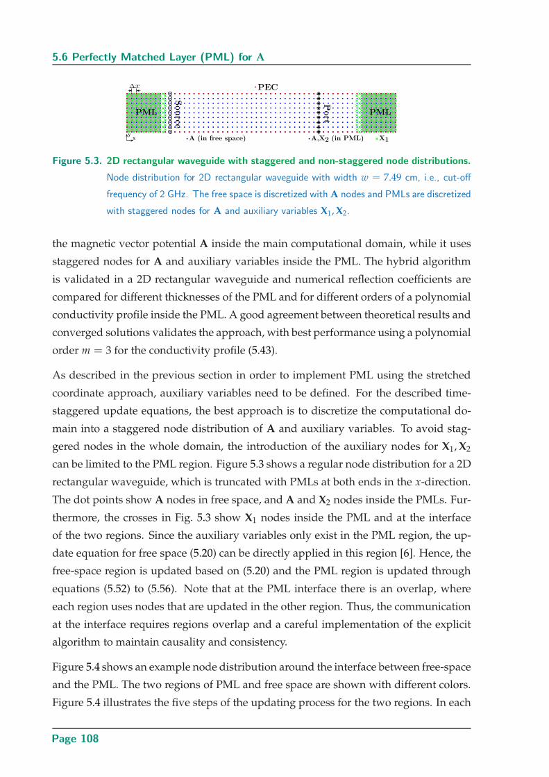
5.6 Perfectly Matched Layer (PML) for A
Figure 5.3. 2D rectangular waveguide with staggered and non-staggered node distributions.
Node distribution for 2D rectangular waveguide with width w = 7.49 cm, i.e., cut-off
frequency of 2 GHz. The free space is discretized with A nodes and PMLs are discretized
with staggered nodes for A and auxiliary variables X1, X2.
the magnetic vector potential A inside the main computational domain, while it uses
staggered nodes for A and auxiliary variables inside the PML. The hybrid algorithm
is validated in a 2D rectangular waveguide and numerical reflection coefficients are
compared for different thicknesses of the PML and for different orders of a polynomial
conductivity profile inside the PML. A good agreement between theoretical results and
converged solutions validates the approach, with best performance using a polynomial
order m = 3 for the conductivity profile (5.43).
As described in the previous section in order to implement PML using the stretched
coordinate approach, auxiliary variables need to be defined. For the described time-
staggered update equations, the best approach is to discretize the computational do-
main into a staggered node distribution of A and auxiliary variables. To avoid stag-
gered nodes in the whole domain, the introduction of the auxiliary nodes for X1, X2
can be limited to the PML region. Figure 5.3 shows a regular node distribution for a 2D
rectangular waveguide, which is truncated with PMLs at both ends in the x-direction.
The dot points show A nodes in free space, and A and X2 nodes inside the PMLs. Fur-
thermore, the crosses in Fig. 5.3 show X1 nodes inside the PML and at the interface
of the two regions. Since the auxiliary variables only exist in the PML region, the up-
date equation for free space (5.20) can be directly applied in this region [6]. Hence, the
free-space region is updated based on (5.20) and the PML region is updated through
equations (5.52) to (5.56). Note that at the PML interface there is an overlap, where
each region uses nodes that are updated in the other region. Thus, the communication
at the interface requires regions overlap and a careful implementation of the explicit
algorithm to maintain causality and consistency.
Figure 5.4 shows an example node distribution around the interface between free-space
and the PML. The two regions of PML and free space are shown with different colors.
Figure 5.4 illustrates the five steps of the updating process for the two regions. In each
Page 108
Chapter 5 Non-Staggered Meshless RPIM: Vector Potential Technique
step, the node to be updated is shown as a darker red point. The updating process is
implemented in five steps as follows
Step 1: The auxiliary variable X1 in the PML (cross points) is updated through vector
potentials A using equation (5.52) (a). As shown in Fig. 5.4.1, the support domain
around each node X1 at the interface includes A nodes in the free-space domain.
The auxiliary variable Y1 is similarly updated through equation (5.53) (a).
Step 2: X2 in the PML is updated using X1 as in (5.52) (b). Y2 is updated similarly
using (5.53) (b).
Step 3: The first-order finite-difference variable DtA in the dot points inside the PML
is calculated using auxiliary variables from the previous step. These values will
be used in Step 5 for updating A in the PML.
Step 4: The magnetic vector potential A in free space is updated through (5.20). As
shown in Fig. 5.4.4, the support domain of each A node in the interface includes
both A nodes from the PML and free-space region.
Step 5: The magnetic vector potential in the PML region is calculated through DtA
which was calculated in Step 3.
This procedure yields a stable hybrid algorithm to link the second-order magnetic vec-
tor potential method and the staggered PML formulation.
5.6.2 Numerical Results
To validate the hybridization algorithm for the staggered and the non-staggered mag-
netic vector potentials in the presence of a PML, the 2D rectangular waveguide struc-
ture shown in Fig. 5.3 is considered. The fundamental TE10 mode distribution is excited
on a source plane as a modulated sinusoidal Gaussian pulse with a spectrum covering
f = [2 − 4] GHz. The structure is discretized with ∆x = λmin/16 and PMLs are used
to truncate the domain on both sides. The theoretical reflection coefficient in (5.44) is
set to R0 = 10−4. To extract the reflection coefficient from the PML, an output port is
defined along the y-axis towards the end of the waveguide as shown in Fig. 5.3. The
S-parameters over the port plane are calculated as in [153].
Figure 5.5 shows the reflection coefficient from the PML with a thickness of d = 10∆x
and different polynomial orders of conductivity profile (5.43) from m = 1 to m = 5
Page 109
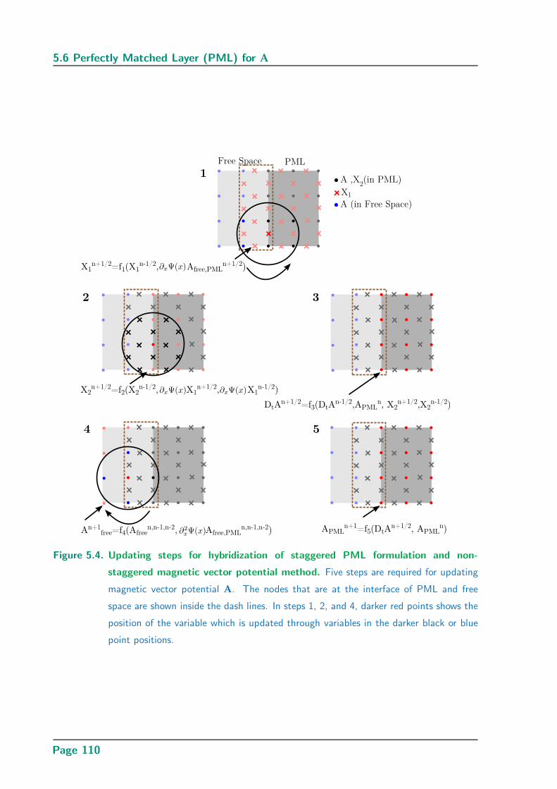
5.6 Perfectly Matched Layer (PML) for A
Figure 5.4. Updating steps for hybridization of staggered PML formulation and non-
staggered magnetic vector potential method. Five steps are required for updating
magnetic vector potential A. The nodes that are at the interface of PML and free
space are shown inside the dash lines. In steps 1, 2, and 4, darker red points shows the
position of the variable which is updated through variables in the darker black or blue
point positions.
Page 110
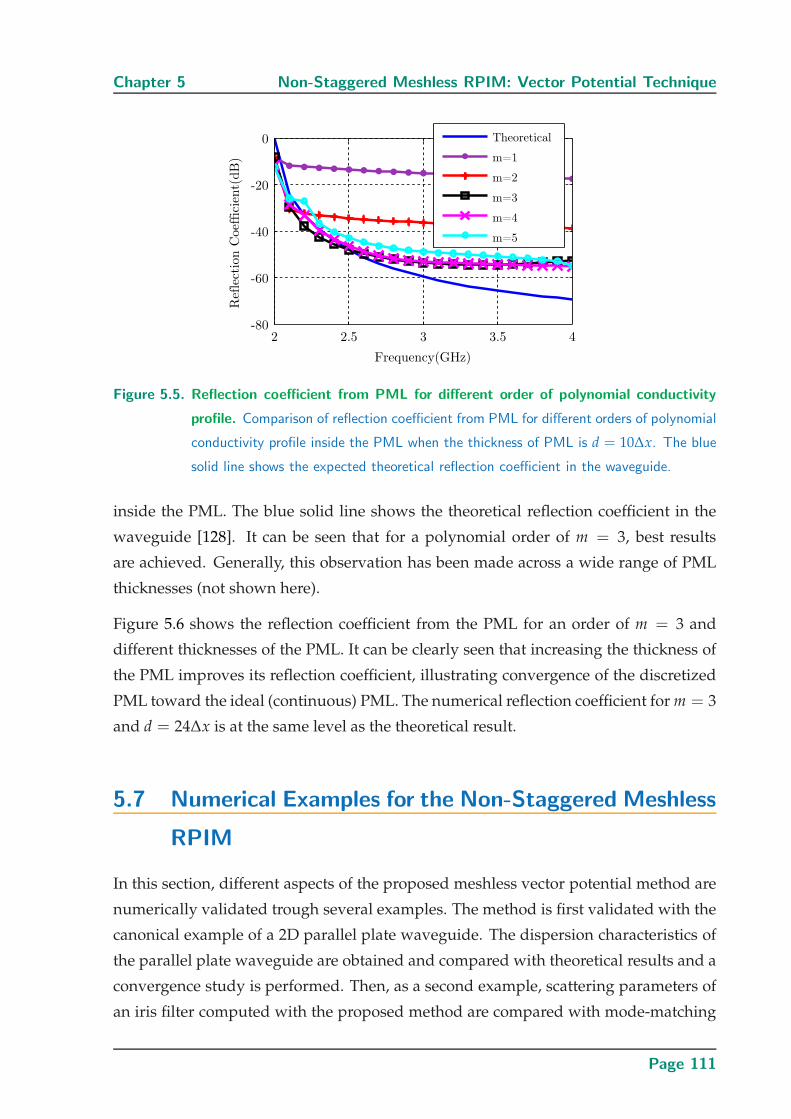
Chapter 5 Non-Staggered Meshless RPIM: Vector Potential Technique
Figure 5.5. Reflection coefficient from PML for different order of polynomial conductivity
profile. Comparison of reflection coefficient from PML for different orders of polynomial
conductivity profile inside the PML when the thickness of PML is d = 10∆x. The blue
solid line shows the expected theoretical reflection coefficient in the waveguide.
inside the PML. The blue solid line shows the theoretical reflection coefficient in the
waveguide [128]. It can be seen that for a polynomial order of m = 3, best results
are achieved. Generally, this observation has been made across a wide range of PML
thicknesses (not shown here).
Figure 5.6 shows the reflection coefficient from the PML for an order of m = 3 and
different thicknesses of the PML. It can be clearly seen that increasing the thickness of
the PML improves its reflection coefficient, illustrating convergence of the discretized
PML toward the ideal (continuous) PML. The numerical reflection coefficient for m = 3
and d = 24∆x is at the same level as the theoretical result.
5.7 Numerical Examples for the Non-Staggered Meshless
RPIM
In this section, different aspects of the proposed meshless vector potential method are
numerically validated trough several examples. The method is first validated with the
canonical example of a 2D parallel plate waveguide. The dispersion characteristics of
the parallel plate waveguide are obtained and compared with theoretical results and a
convergence study is performed. Then, as a second example, scattering parameters of
an iris filter computed with the proposed method are compared with mode-matching
Page 111
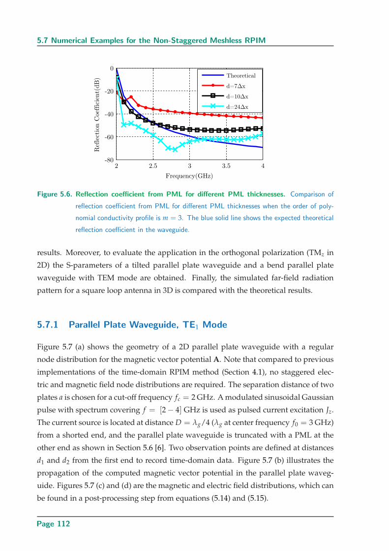
5.7 Numerical Examples for the Non-Staggered Meshless RPIM
Figure 5.6. Reflection coefficient from PML for different PML thicknesses. Comparison of
reflection coefficient from PML for different PML thicknesses when the order of poly-
nomial conductivity profile is m = 3. The blue solid line shows the expected theoretical
reflection coefficient in the waveguide.
results. Moreover, to evaluate the application in the orthogonal polarization (TMz in
2D) the S-parameters of a tilted parallel plate waveguide and a bend parallel plate
waveguide with TEM mode are obtained. Finally, the simulated far-field radiation
pattern for a square loop antenna in 3D is compared with the theoretical results.
5.7.1 Parallel Plate Waveguide, TE1 Mode
Figure 5.7 (a) shows the geometry of a 2D parallel plate waveguide with a regular
node distribution for the magnetic vector potential A. Note that compared to previous
implementations of the time-domain RPIM method (Section 4.1), no staggered elec-
tric and magnetic field node distributions are required. The separation distance of two
plates a is chosen for a cut-off frequency fc = 2 GHz. A modulated sinusoidal Gaussian
pulse with spectrum covering f = [2 − 4] GHz is used as pulsed current excitation Jz.
The current source is located at distance D = λg/4 (λg at center frequency f0 = 3 GHz)
from a shorted end, and the parallel plate waveguide is truncated with a PML at the
other end as shown in Section 5.6 [6]. Two observation points are defined at distances
d1 and d2 from the first end to record time-domain data. Figure 5.7 (b) illustrates the
propagation of the computed magnetic vector potential in the parallel plate waveg-
uide. Figures 5.7 (c) and (d) are the magnetic and electric field distributions, which can
be found in a post-processing step from equations (5.14) and (5.15).
Page 112
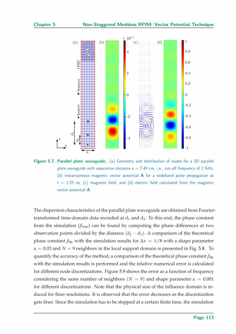
Chapter 5 Non-Staggered Meshless RPIM: Vector Potential Technique
Figure 5.7. Parallel plate waveguide. (a) Geometry and distribution of nodes for a 2D parallel
plate waveguide with separation distance a = 7.49 cm, i.e., cut-off frequency of 2 GHz,
(b) instantaneous magnetic vector potential A for a wideband pulse propagation at
t = 1.53 ns, (c) magnetic field, and (d) electric field calculated from the magnetic
vector potential A.
The dispersion characteristics of the parallel plate waveguide are obtained from Fourier-
transformed time-domain data recorded at d1 and d2. To this end, the phase constant
from the simulation (βsim) can be found by computing the phase differences at two
observation points divided by the distance (d2 − d1). A comparison of the theoretical
phase constant βth with the simulation results for ∆x = λ/8 with a shape parameter
α = 0.03 and N = 9 neighbors in the local support domain is presented in Fig. 5.8. To
quantify the accuracy of the method, a comparison of the theoretical phase constant βth
with the simulation results is performed and the relative numerical error is calculated
for different node discretizations. Figure 5.9 shows the error as a function of frequency
considering the same number of neighbors (N = 9) and shape parameter α = 0.001
for different discretizations. Note that the physical size of the influence domain is re-
duced for finer resolutions. It is observed that the error decreases as the discretization
gets finer. Since the simulation has to be stopped at a certain finite time, the simulation
Page 113
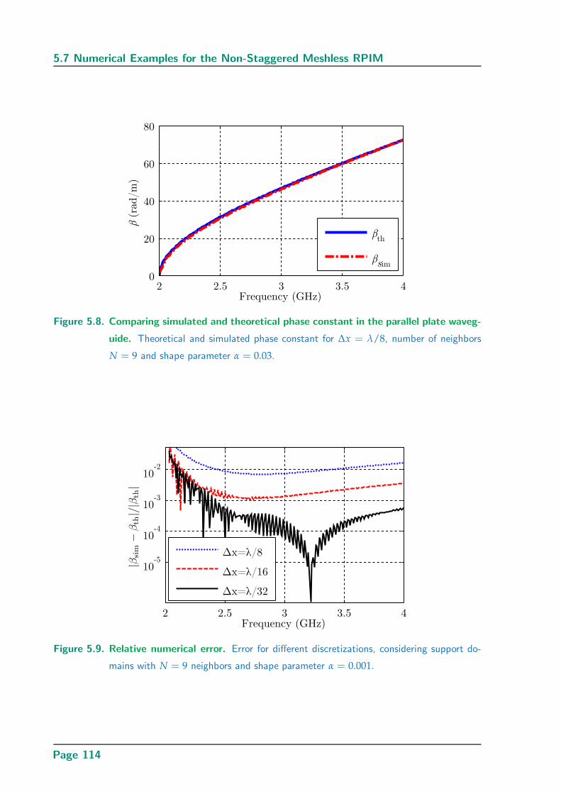
5.7 Numerical Examples for the Non-Staggered Meshless RPIM
Figure 5.8. Comparing simulated and theoretical phase constant in the parallel plate waveg-
uide. Theoretical and simulated phase constant for ∆x = λ/8, number of neighbors
N = 9 and shape parameter α = 0.03.
Figure 5.9. Relative numerical error. Error for different discretizations, considering support do-
mains with N = 9 neighbors and shape parameter α = 0.001.
Page 114
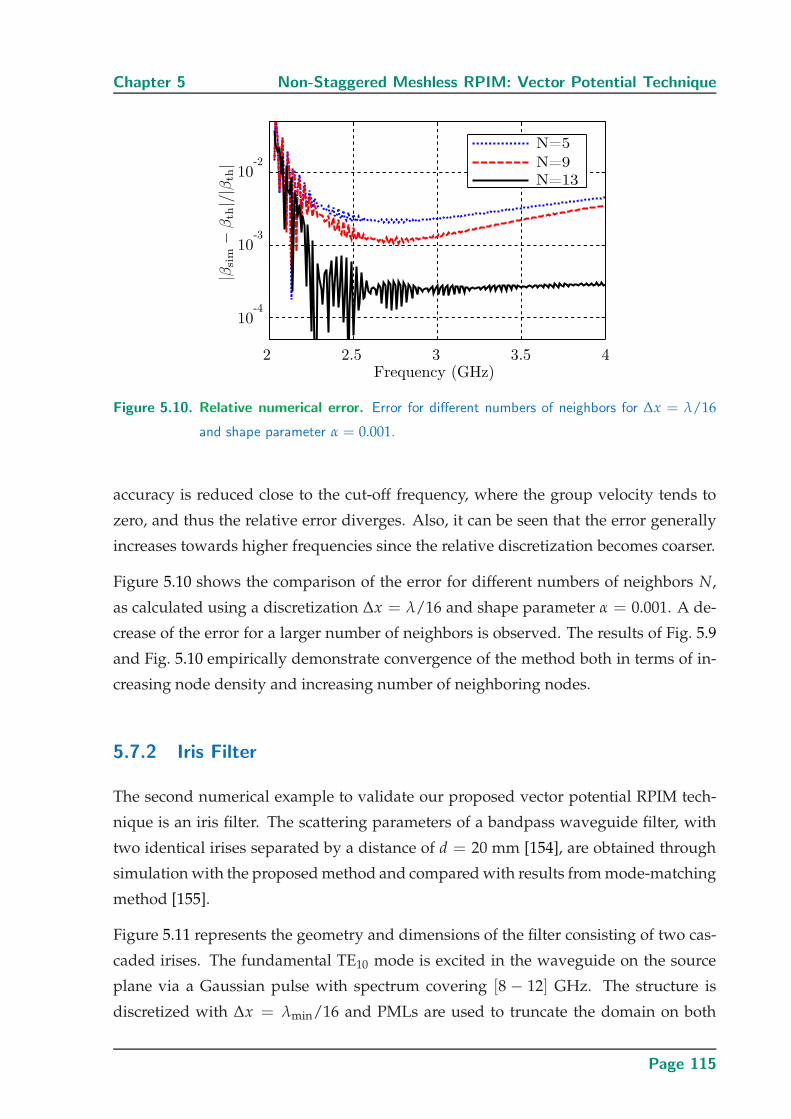
Chapter 5 Non-Staggered Meshless RPIM: Vector Potential Technique
Figure 5.10. Relative numerical error. Error for different numbers of neighbors for ∆x = λ/16
and shape parameter α = 0.001.
accuracy is reduced close to the cut-off frequency, where the group velocity tends to
zero, and thus the relative error diverges. Also, it can be seen that the error generally
increases towards higher frequencies since the relative discretization becomes coarser.
Figure 5.10 shows the comparison of the error for different numbers of neighbors N,
as calculated using a discretization ∆x = λ/16 and shape parameter α = 0.001. A de-
crease of the error for a larger number of neighbors is observed. The results of Fig. 5.9
and Fig. 5.10 empirically demonstrate convergence of the method both in terms of in-
creasing node density and increasing number of neighboring nodes.
5.7.2 Iris Filter
The second numerical example to validate our proposed vector potential RPIM tech-
nique is an iris filter. The scattering parameters of a bandpass waveguide filter, with
two identical irises separated by a distance of d = 20 mm [154], are obtained through
simulation with the proposed method and compared with results from mode-matching
method [155].
Figure 5.11 represents the geometry and dimensions of the filter consisting of two cas-
caded irises. The fundamental TE10 mode is excited in the waveguide on the source
plane via a Gaussian pulse with spectrum covering [8 − 12] GHz. The structure is
discretized with ∆x = λmin/16 and PMLs are used to truncate the domain on both
Page 115
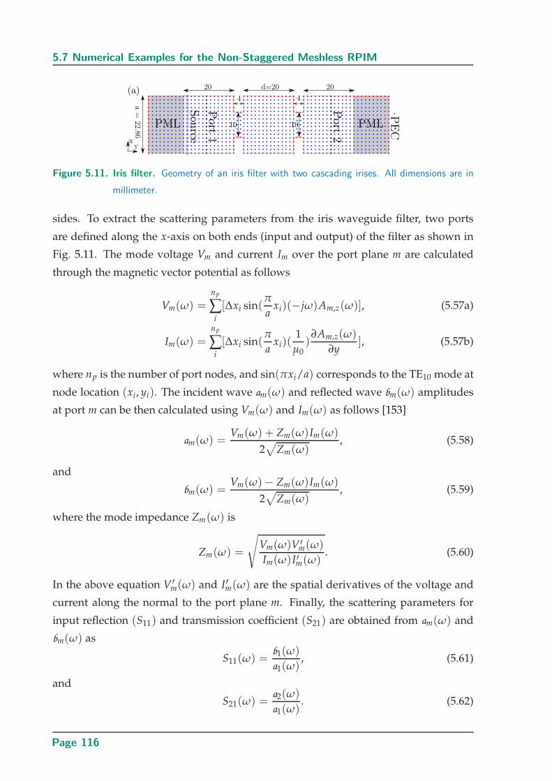
5.7 Numerical Examples for the Non-Staggered Meshless RPIM
Figure 5.11. Iris filter. Geometry of an iris filter with two cascading irises. All dimensions are in
millimeter.
sides. To extract the scattering parameters from the iris waveguide filter, two ports
are defined along the x-axis on both ends (input and output) of the filter as shown in
Fig. 5.11. The mode voltage Vm and current Im over the port plane m are calculated
through the magnetic vector potential as follows
Vm(ω) =np
∑i
[∆xi sin(π
axi)(−jω)Am,z(ω)], (5.57a)
Im(ω) =np
∑i
[∆xi sin(π
axi)(
1
µ0)
∂Am,z(ω)
∂y], (5.57b)
where np is the number of port nodes, and sin(πxi/a) corresponds to the TE10 mode at
node location (xi, yi). The incident wave am(ω) and reflected wave bm(ω) amplitudes
at port m can be then calculated using Vm(ω) and Im(ω) as follows [153]
am(ω) =Vm(ω) + Zm(ω)Im(ω)
2√
Zm(ω), (5.58)
and
bm(ω) =Vm(ω)− Zm(ω)Im(ω)
2√
Zm(ω), (5.59)
where the mode impedance Zm(ω) is
Zm(ω) =
√Vm(ω)V ′
m(ω)
Im(ω)I ′m(ω). (5.60)
In the above equation V ′m(ω) and I ′m(ω) are the spatial derivatives of the voltage and
current along the normal to the port plane m. Finally, the scattering parameters for
input reflection (S11) and transmission coefficient (S21) are obtained from am(ω) and
bm(ω) as
S11(ω) =b1(ω)
a1(ω), (5.61)
and
S21(ω) =a2(ω)
a1(ω). (5.62)
Page 116
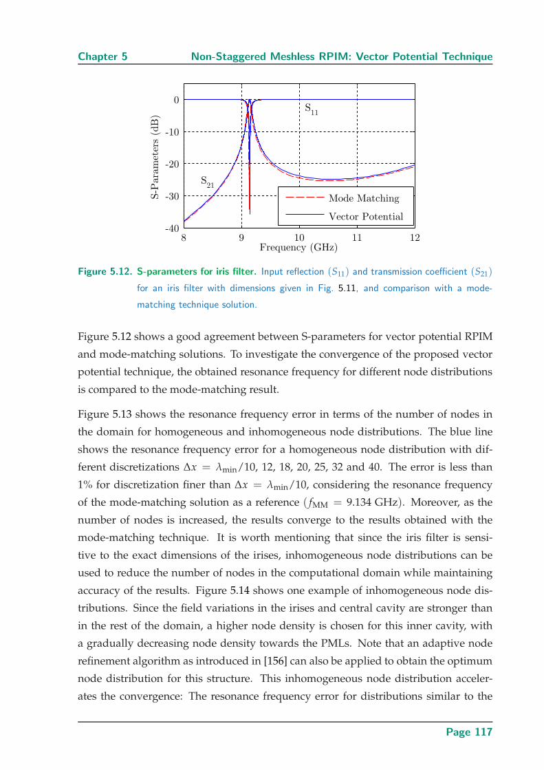
Chapter 5 Non-Staggered Meshless RPIM: Vector Potential Technique
Figure 5.12. S-parameters for iris filter. Input reflection (S11) and transmission coefficient (S21)
for an iris filter with dimensions given in Fig. 5.11, and comparison with a mode-
matching technique solution.
Figure 5.12 shows a good agreement between S-parameters for vector potential RPIM
and mode-matching solutions. To investigate the convergence of the proposed vector
potential technique, the obtained resonance frequency for different node distributions
is compared to the mode-matching result.
Figure 5.13 shows the resonance frequency error in terms of the number of nodes in
the domain for homogeneous and inhomogeneous node distributions. The blue line
shows the resonance frequency error for a homogeneous node distribution with dif-
ferent discretizations ∆x = λmin/10, 12, 18, 20, 25, 32 and 40. The error is less than
1% for discretization finer than ∆x = λmin/10, considering the resonance frequency
of the mode-matching solution as a reference ( fMM = 9.134 GHz). Moreover, as the
number of nodes is increased, the results converge to the results obtained with the
mode-matching technique. It is worth mentioning that since the iris filter is sensi-
tive to the exact dimensions of the irises, inhomogeneous node distributions can be
used to reduce the number of nodes in the computational domain while maintaining
accuracy of the results. Figure 5.14 shows one example of inhomogeneous node dis-
tributions. Since the field variations in the irises and central cavity are stronger than
in the rest of the domain, a higher node density is chosen for this inner cavity, with
a gradually decreasing node density towards the PMLs. Note that an adaptive node
refinement algorithm as introduced in [156] can also be applied to obtain the optimum
node distribution for this structure. This inhomogeneous node distribution acceler-
ates the convergence: The resonance frequency error for distributions similar to the
Page 117
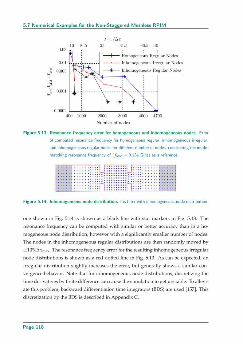
5.7 Numerical Examples for the Non-Staggered Meshless RPIM
Figure 5.13. Resonance frequency error for homogeneous and inhomogeneous nodes. Error
of computed resonance frequency for homogeneous regular, inhomogeneous irregular,
and inhomogeneous regular nodes for different number of nodes, considering the mode-
matching resonance frequency of ( fMM = 9.134 GHz) as a reference.
Figure 5.14. Inhomogeneous node distribution. Iris filter with inhomogeneous node distribution.
one shown in Fig. 5.14 is shown as a black line with star markers in Fig. 5.13. The
resonance frequency can be computed with similar or better accuracy than in a ho-
mogeneous node distribution, however with a significantly smaller number of nodes.
The nodes in the inhomogeneous regular distributions are then randomly moved by
±10%∆xmax. The resonance frequency error for the resulting inhomogeneous irregular
node distributions is shown as a red dotted line in Fig. 5.13. As can be expected, an
irregular distribution slightly increases the error, but generally shows a similar con-
vergence behavior. Note that for inhomogeneous node distributions, discretizing the
time derivatives by finite difference can cause the simulation to get unstable. To allevi-
ate this problem, backward differentiation time integrators (BDS) are used [157]. This
discretization by the BDS is described in Appendix C.
Page 118
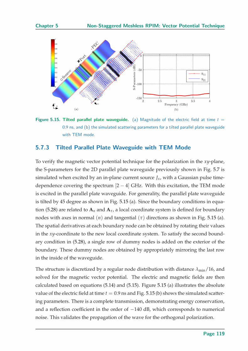
Chapter 5 Non-Staggered Meshless RPIM: Vector Potential Technique
Figure 5.15. Tilted parallel plate waveguide. (a) Magnitude of the electric field at time t =
0.9 ns, and (b) the simulated scattering parameters for a tilted parallel plate waveguide
with TEM mode.
5.7.3 Tilted Parallel Plate Waveguide with TEM Mode
To verify the magnetic vector potential technique for the polarization in the xy-plane,
the S-parameters for the 2D parallel plate waveguide previously shown in Fig. 5.7 is
simulated when excited by an in-plane current source Jx, with a Gaussian pulse time-
dependence covering the spectrum [2 − 4] GHz. With this excitation, the TEM mode
is excited in the parallel plate waveguide. For generality, the parallel plate waveguide
is tilted by 45 degree as shown in Fig. 5.15 (a). Since the boundary conditions in equa-
tion (5.28) are related to An and Aτ, a local coordinate system is defined for boundary
nodes with axes in normal (n) and tangential (τ) directions as shown in Fig. 5.15 (a).
The spatial derivatives at each boundary node can be obtained by rotating their values
in the xy-coordinate to the new local coordinate system. To satisfy the second bound-
ary condition in (5.28), a single row of dummy nodes is added on the exterior of the
boundary. These dummy nodes are obtained by appropriately mirroring the last row
in the inside of the waveguide.
The structure is discretized by a regular node distribution with distance λmin/16, and
solved for the magnetic vector potential. The electric and magnetic fields are then
calculated based on equations (5.14) and (5.15). Figure 5.15 (a) illustrates the absolute
value of the electric field at time t = 0.9 ns and Fig. 5.15 (b) shows the simulated scatter-
ing parameters. There is a complete transmission, demonstrating energy conservation,
and a reflection coefficient in the order of −140 dB, which corresponds to numerical
noise. This validates the propagation of the wave for the orthogonal polarization.
Page 119
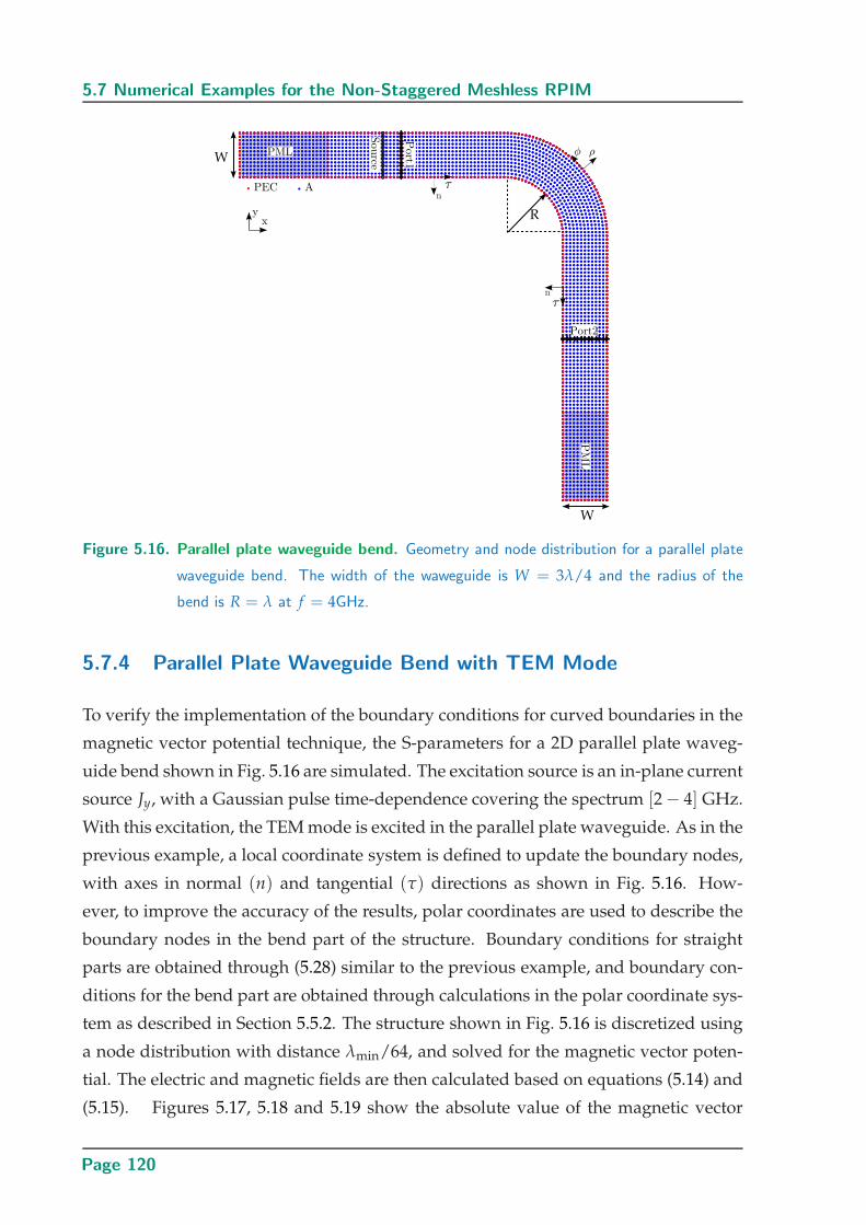
5.7 Numerical Examples for the Non-Staggered Meshless RPIM
Figure 5.16. Parallel plate waveguide bend. Geometry and node distribution for a parallel plate
waveguide bend. The width of the waweguide is W = 3λ/4 and the radius of the
bend is R = λ at f = 4GHz.
5.7.4 Parallel Plate Waveguide Bend with TEM Mode
To verify the implementation of the boundary conditions for curved boundaries in the
magnetic vector potential technique, the S-parameters for a 2D parallel plate waveg-
uide bend shown in Fig. 5.16 are simulated. The excitation source is an in-plane current
source Jy, with a Gaussian pulse time-dependence covering the spectrum [2 − 4] GHz.
With this excitation, the TEM mode is excited in the parallel plate waveguide. As in the
previous example, a local coordinate system is defined to update the boundary nodes,
with axes in normal (n) and tangential (τ) directions as shown in Fig. 5.16. How-
ever, to improve the accuracy of the results, polar coordinates are used to describe the
boundary nodes in the bend part of the structure. Boundary conditions for straight
parts are obtained through (5.28) similar to the previous example, and boundary con-
ditions for the bend part are obtained through calculations in the polar coordinate sys-
tem as described in Section 5.5.2. The structure shown in Fig. 5.16 is discretized using
a node distribution with distance λmin/64, and solved for the magnetic vector poten-
tial. The electric and magnetic fields are then calculated based on equations (5.14) and
(5.15). Figures 5.17, 5.18 and 5.19 show the absolute value of the magnetic vector
Page 120
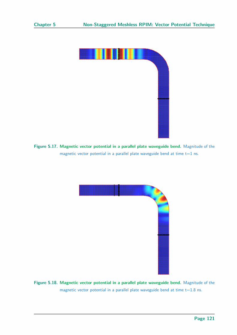
Chapter 5 Non-Staggered Meshless RPIM: Vector Potential Technique
Figure 5.17. Magnetic vector potential in a parallel plate waveguide bend. Magnitude of the
magnetic vector potential in a parallel plate waveguide bend at time t=1 ns.
Figure 5.18. Magnetic vector potential in a parallel plate waveguide bend. Magnitude of the
magnetic vector potential in a parallel plate waveguide bend at time t=1.8 ns.
Page 121
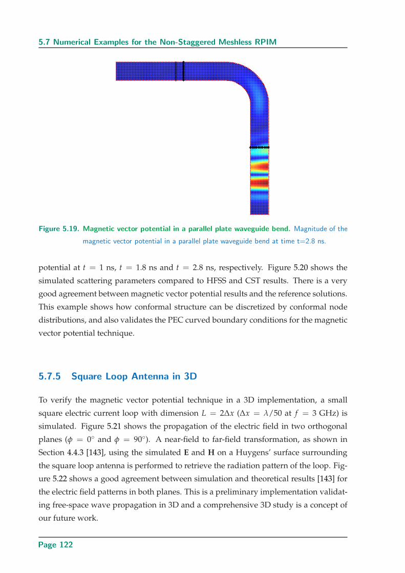
5.7 Numerical Examples for the Non-Staggered Meshless RPIM
Figure 5.19. Magnetic vector potential in a parallel plate waveguide bend. Magnitude of the
magnetic vector potential in a parallel plate waveguide bend at time t=2.8 ns.
potential at t = 1 ns, t = 1.8 ns and t = 2.8 ns, respectively. Figure 5.20 shows the
simulated scattering parameters compared to HFSS and CST results. There is a very
good agreement between magnetic vector potential results and the reference solutions.
This example shows how conformal structure can be discretized by conformal node
distributions, and also validates the PEC curved boundary conditions for the magnetic
vector potential technique.
5.7.5 Square Loop Antenna in 3D
To verify the magnetic vector potential technique in a 3D implementation, a small
square electric current loop with dimension L = 2∆x (∆x = λ/50 at f = 3 GHz) is
simulated. Figure 5.21 shows the propagation of the electric field in two orthogonal
planes (φ = 0 and φ = 90). A near-field to far-field transformation, as shown in
Section 4.4.3 [143], using the simulated E and H on a Huygens’ surface surrounding
the square loop antenna is performed to retrieve the radiation pattern of the loop. Fig-
ure 5.22 shows a good agreement between simulation and theoretical results [143] for
the electric field patterns in both planes. This is a preliminary implementation validat-
ing free-space wave propagation in 3D and a comprehensive 3D study is a concept of
our future work.
Page 122
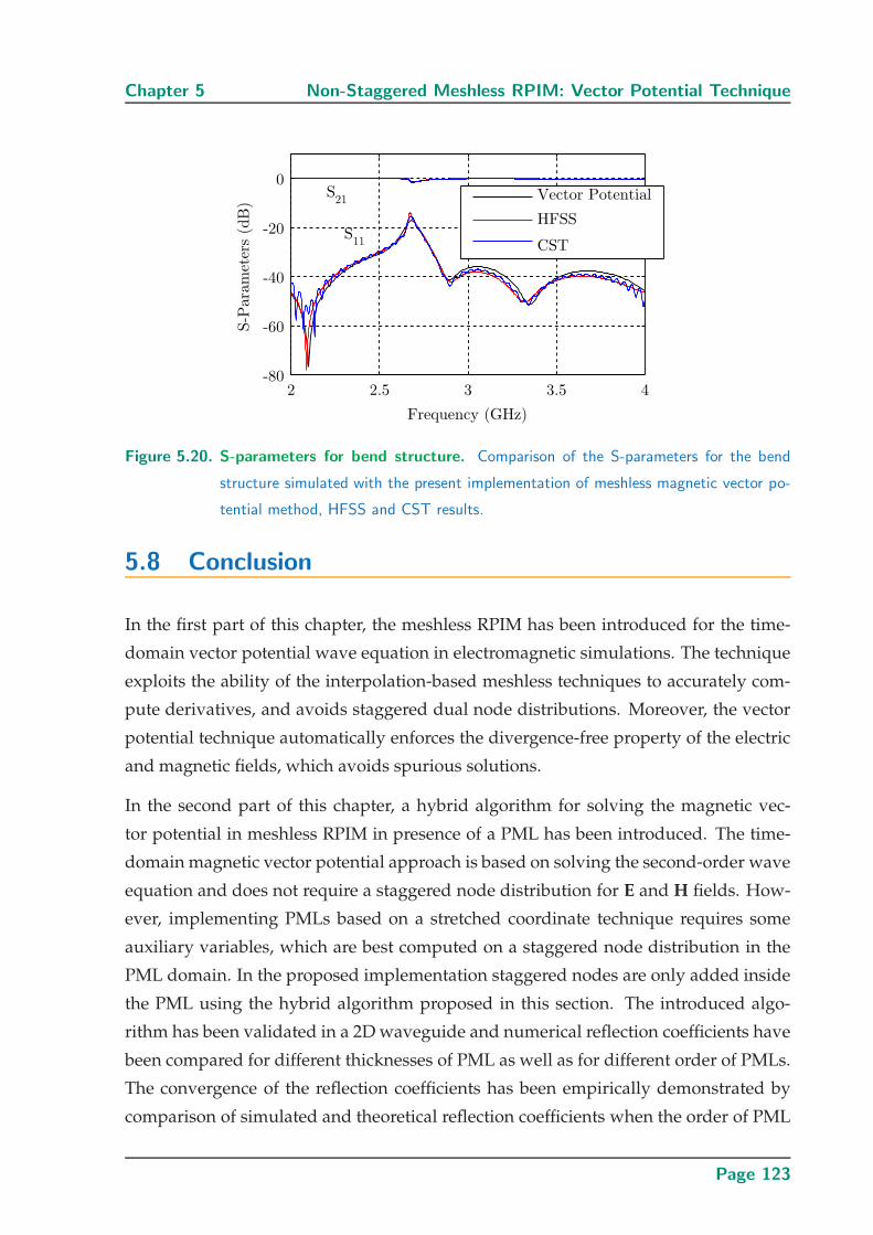
Chapter 5 Non-Staggered Meshless RPIM: Vector Potential Technique
Figure 5.20. S-parameters for bend structure. Comparison of the S-parameters for the bend
structure simulated with the present implementation of meshless magnetic vector po-
tential method, HFSS and CST results.
5.8 Conclusion
In the first part of this chapter, the meshless RPIM has been introduced for the time-
domain vector potential wave equation in electromagnetic simulations. The technique
exploits the ability of the interpolation-based meshless techniques to accurately com-
pute derivatives, and avoids staggered dual node distributions. Moreover, the vector
potential technique automatically enforces the divergence-free property of the electric
and magnetic fields, which avoids spurious solutions.
In the second part of this chapter, a hybrid algorithm for solving the magnetic vec-
tor potential in meshless RPIM in presence of a PML has been introduced. The time-
domain magnetic vector potential approach is based on solving the second-order wave
equation and does not require a staggered node distribution for E and H fields. How-
ever, implementing PMLs based on a stretched coordinate technique requires some
auxiliary variables, which are best computed on a staggered node distribution in the
PML domain. In the proposed implementation staggered nodes are only added inside
the PML using the hybrid algorithm proposed in this section. The introduced algo-
rithm has been validated in a 2D waveguide and numerical reflection coefficients have
been compared for different thicknesses of PML as well as for different order of PMLs.
The convergence of the reflection coefficients has been empirically demonstrated by
comparison of simulated and theoretical reflection coefficients when the order of PML
Page 123
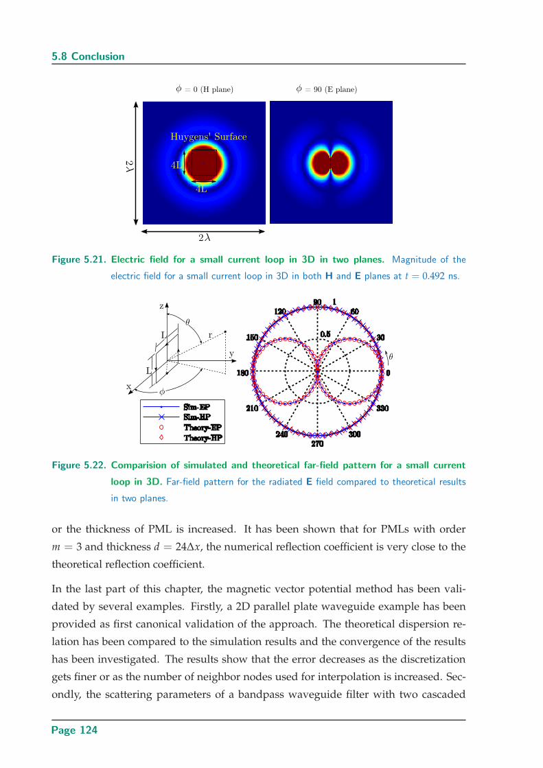
5.8 Conclusion
Figure 5.21. Electric field for a small current loop in 3D in two planes. Magnitude of the
electric field for a small current loop in 3D in both H and E planes at t = 0.492 ns.
Figure 5.22. Comparision of simulated and theoretical far-field pattern for a small current
loop in 3D. Far-field pattern for the radiated E field compared to theoretical results
in two planes.
or the thickness of PML is increased. It has been shown that for PMLs with order
m = 3 and thickness d = 24∆x, the numerical reflection coefficient is very close to the
theoretical reflection coefficient.
In the last part of this chapter, the magnetic vector potential method has been vali-
dated by several examples. Firstly, a 2D parallel plate waveguide example has been
provided as first canonical validation of the approach. The theoretical dispersion re-
lation has been compared to the simulation results and the convergence of the results
has been investigated. The results show that the error decreases as the discretization
gets finer or as the number of neighbor nodes used for interpolation is increased. Sec-
ondly, the scattering parameters of a bandpass waveguide filter with two cascaded
Page 124
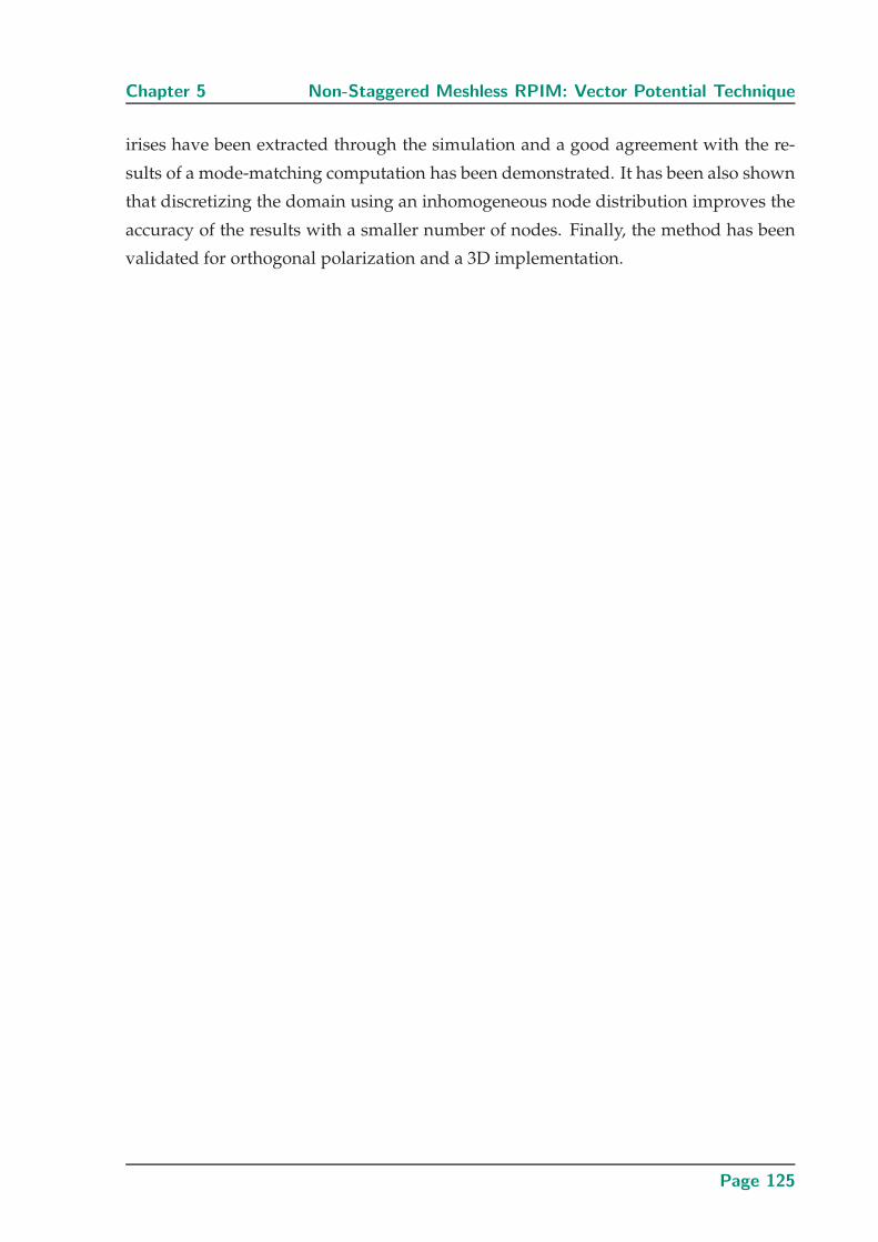
Chapter 5 Non-Staggered Meshless RPIM: Vector Potential Technique
irises have been extracted through the simulation and a good agreement with the re-
sults of a mode-matching computation has been demonstrated. It has been also shown
that discretizing the domain using an inhomogeneous node distribution improves the
accuracy of the results with a smaller number of nodes. Finally, the method has been
validated for orthogonal polarization and a 3D implementation.
Page 125

Page 126
Chapter 6
Comparing Staggered andNon-Staggered Meshless
RPIM
THIS chapter directly compares the staggered and non-staggered
algorithms of meshless methods presented in the previous parts
of this thesis. In the first part, the salient features of both algo-
rithms are briefly recapitulated. This starts with the Radial Point Interpola-
tion Method (RPIM) to solve the E and H fields in a staggered node arrange-
ments. Then, the solver for the second-order vector potential wave equation
is summarized. The second algorithm avoids ambiguity and effort related
to a dual node distribution required for solving the first-order Maxwell’s
equations. In the second part of the chapter, the actual direct comparison
between the staggered and non-staggered RPIM for time-domain electro-
magnetics is performed. As illustrative example, the scattering parameters
of a waveguide filter are computed using both staggered and non-staggered
RPIM. The accuracy of the results obtained with both methods is assessed
through comparison with a reference solution.
Page 127
6.1 Introduction
6.1 Introduction
Time-domain meshless methods in electromagnetics have been introduced for field
computations in staggered node distributions for electric and magnetic fields, i.e., for
the first-order Maxwell’s equations in [20, 21, 22, 158] and an implementation of 3D
staggered Radial Point Interpolation Method (RPIM) has been described in Chapter 4.
However, generating unstructured dual node distributions for the electric and mag-
netic fields increase the computational load and can decrease the accuracy of the re-
sults. Moreover, the need of a staggered node distribution restricts the freedom of
node positions in meshless methods and might reduce the potential advantages of the
method.
To overcome this problem, a meshless vector potential technique can be used to solve
electromagnetic problems. Although the order of the partial differential equations is
increased to second order compared to the first-order Maxwell’s equations, the numeri-
cal errors for a given space discretization can be decreased in vector potential methods.
Moreover, in this formalism fields can be described using three scalar wave equations,
and it has been shown in [27] that less CPU time is needed for the vector potential
FDTD method compared to the classical staggered approach. An implementation of
the time-domain meshless RPIM based on the local calculation of the magnetic vector
potential (A) in small support domains has been introduced in Chapter 5.
In this chapter, staggered and non-staggered meshless RPIM are directly compared.
To this end, the main features of staggered and non-staggered meshless RPIM are first
recapitulated briefly, and then these two methods are compared using illustrative nu-
merical results.
As shown in Chapter 3, in RPIM the approximation of the field value u(x) and its
derivatives at position x is given by
uh(x) = [φ1(x), φ2(x), ..., φN(x)]Ue , (6.1a)
∂uh(x)
∂k= [
∂φ1(x)
∂k,
∂φ2(x)
∂k, ...,
∂φN(x)
∂k]Ue, (6.1b)
∂2uh(x)
∂k2= [
∂2φ1(x)
∂k2,
∂2φ2(x)
∂k2, ...,
∂2φN(x)
∂k2]Ue, (6.1c)
where Ue is the field value at N surrounding nodes and φi(x) are the shape functions,
which can be computed using radial basis functions in a pre-processing step.
These approximations are used in the following to summarize the implementation of
the staggered and non-staggered meshless RPIM.
Page 128
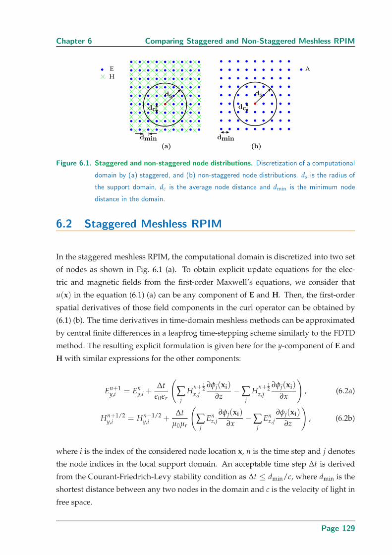
Chapter 6 Comparing Staggered and Non-Staggered Meshless RPIM
Figure 6.1. Staggered and non-staggered node distributions. Discretization of a computational
domain by (a) staggered, and (b) non-staggered node distributions. ds is the radius of
the support domain, dc is the average node distance and dmin is the minimum node
distance in the domain.
6.2 Staggered Meshless RPIM
In the staggered meshless RPIM, the computational domain is discretized into two set
of nodes as shown in Fig. 6.1 (a). To obtain explicit update equations for the elec-
tric and magnetic fields from the first-order Maxwell’s equations, we consider that
u(x) in the equation (6.1) (a) can be any component of E and H. Then, the first-order
spatial derivatives of those field components in the curl operator can be obtained by
(6.1) (b). The time derivatives in time-domain meshless methods can be approximated
by central finite differences in a leapfrog time-stepping scheme similarly to the FDTD
method. The resulting explicit formulation is given here for the y-component of E and
H with similar expressions for the other components:
En+1y,i = En
y,i +∆t
ǫ0ǫr
(
∑j
Hn+ 1
2x,j
∂φj(xi)
∂z− ∑
j
Hn+ 1
2z,j
∂φj(xi)
∂x
), (6.2a)
Hn+1/2y,i = Hn−1/2
y,i +∆t
µ0µr
(
∑j
Enz,j
∂φj(xi)
∂x−∑
j
Enx,j
∂φj(xi)
∂z
), (6.2b)
where i is the index of the considered node location x, n is the time step and j denotes
the node indices in the local support domain. An acceptable time step ∆t is derived
from the Courant-Friedrich-Levy stability condition as ∆t ≤ dmin/c, where dmin is the
shortest distance between any two nodes in the domain and c is the velocity of light in
free space.
Page 129
6.3 Non-Staggered Meshless RPIM
6.3 Non-Staggered Meshless RPIM
In the magnetic vector potential technique, the computational domain is discretized
into one set of nodes for the vector potential A as shown in Fig. 6.1 (b). The discretized
second-order wave equation is numerically solved on that node distribution. The mag-
netic vector potential is defined by
B = ∇× A, (6.3)
and the electric and magnetic fields from Maxwell’s equations are related to A as
E = −∂A
∂t+
1
µǫ
∫∇∇ · Adt, (6.4)
and
H =1
µ(∇× A). (6.5)
The electric field in (6.4) is obtained through the Lorenz gauge condition. In the pres-
ence of a current source J, the magnetic vector potential satisfies the inhomogeneous
wave equation as
∇2A − µǫ∂2A
∂t2= −µJ. (6.6)
Note that in the presence of magnetic sources, the wave equation for the electric vector
potential F can be obtained in a similar way as the magnetic vector potential A. As
mentioned before, the simulation for the electric vector potential F could be made in
parallel to the A, and on the same node distribution.
Using RPIM to discretize space derivatives and finite differences to discretize time
derivatives in (6.6) lead to the discretized expression for the magnetic vector potential.
In other words, u(x) can be considered as magnetic vector potential and the second
spatial derivatives of each magnetic vector potential components can be obtained by
(6.1) (c). The second-order time-derivatives in the time-domain wave equation can be
approximated by conditionally stable second-order central differences. In this chapter,
a 2D framework with the magnetic vector potential perpendicular to the xy-plane and
constant in the z-direction is considered. According to (6.5) and (6.4), the correspond-
ing magnetic field is in the xy-plane, and the corresponding electric field is along z.
The update equations for the magnetic vector potential in this case can be derived as
An+1z = 2An
z − An−1z +
(∆t)2
µǫ
(∂2φ(x)
∂x2An
z +∂2φ(x)
∂y2An
z
)+
(∆t)2
ǫJnz . (6.7)
Page 130
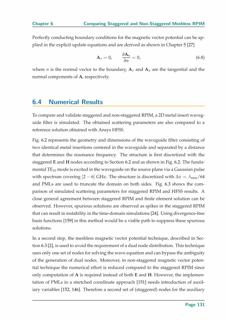
Chapter 6 Comparing Staggered and Non-Staggered Meshless RPIM
Perfectly conducting boundary conditions for the magnetic vector potential can be ap-
plied in the explicit update equations and are derived as shown in Chapter 5 [27]
Aτ = 0,∂An
∂n= 0, (6.8)
where n is the normal vector to the boundary, Aτ and An are the tangential and the
normal components of A, respectively.
6.4 Numerical Results
To compare and validate staggered and non-staggered RPIM, a 2D metal insert waveg-
uide filter is simulated. The obtained scattering parameters are also compared to a
reference solution obtained with Ansys HFSS.
Fig. 6.2 represents the geometry and dimensions of the waveguide filter consisting of
two identical metal insertions centered in the waveguide and separated by a distance
that determines the resonance frequency. The structure is first discretized with the
staggered E and H nodes according to Section 6.2 and as shown in Fig. 6.2. The funda-
mental TE10 mode is excited in the waveguide on the source plane via a Gaussian pulse
with spectrum covering [2 − 6] GHz. The structure is discretized with ∆x = λmin/64
and PMLs are used to truncate the domain on both sides. Fig. 6.3 shows the com-
parison of simulated scattering parameters for staggered RPIM and HFSS results. A
close general agreement between staggered RPIM and finite element solution can be
observed. However, spurious solutions are observed as spikes in the staggered RPIM
that can result in instability in the time-domain simulations [24]. Using divergence-free
basis functions [159] in this method would be a viable path to suppress these spurious
solutions.
In a second step, the meshless magnetic vector potential technique, described in Sec-
tion 6.3 [2], is used to avoid the requirement of a dual node distribution. This technique
uses only one set of nodes for solving the wave equation and can bypass the ambiguity
of the generation of dual nodes. Moreover, in non-staggered magnetic vector poten-
tial technique the numerical effort is reduced compared to the staggered RPIM since
only computation of A is required instead of both E and H. However, the implemen-
tation of PMLs in a stretched coordinate approach [151] needs introduction of auxil-
iary variables [152, 146]. Therefore a second set of (staggered) nodes for the auxiliary
Page 131
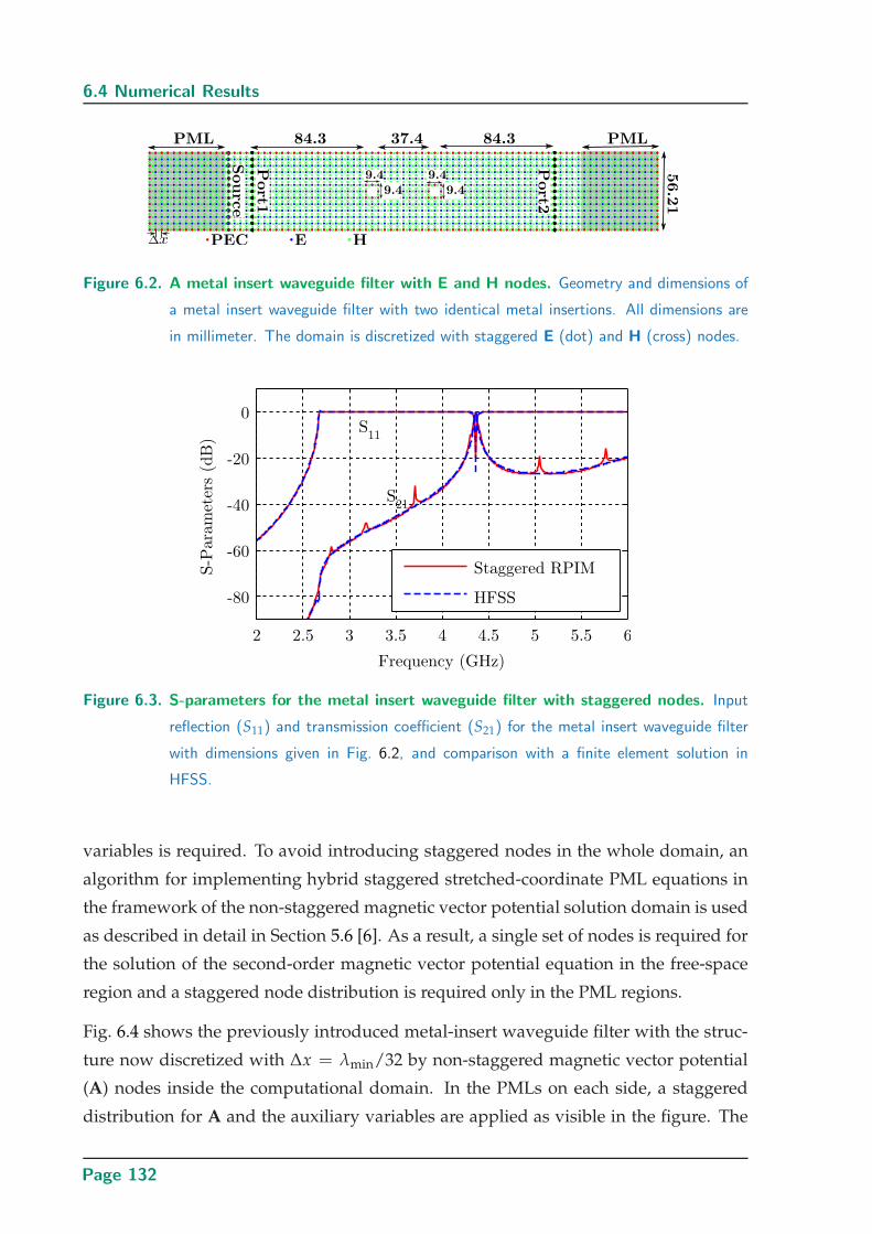
6.4 Numerical Results
Figure 6.2. A metal insert waveguide filter with E and H nodes. Geometry and dimensions of
a metal insert waveguide filter with two identical metal insertions. All dimensions are
in millimeter. The domain is discretized with staggered E (dot) and H (cross) nodes.
Figure 6.3. S-parameters for the metal insert waveguide filter with staggered nodes. Input
reflection (S11) and transmission coefficient (S21) for the metal insert waveguide filter
with dimensions given in Fig. 6.2, and comparison with a finite element solution in
HFSS.
variables is required. To avoid introducing staggered nodes in the whole domain, an
algorithm for implementing hybrid staggered stretched-coordinate PML equations in
the framework of the non-staggered magnetic vector potential solution domain is used
as described in detail in Section 5.6 [6]. As a result, a single set of nodes is required for
the solution of the second-order magnetic vector potential equation in the free-space
region and a staggered node distribution is required only in the PML regions.
Fig. 6.4 shows the previously introduced metal-insert waveguide filter with the struc-
ture now discretized with ∆x = λmin/32 by non-staggered magnetic vector potential
(A) nodes inside the computational domain. In the PMLs on each side, a staggered
distribution for A and the auxiliary variables are applied as visible in the figure. The
Page 132
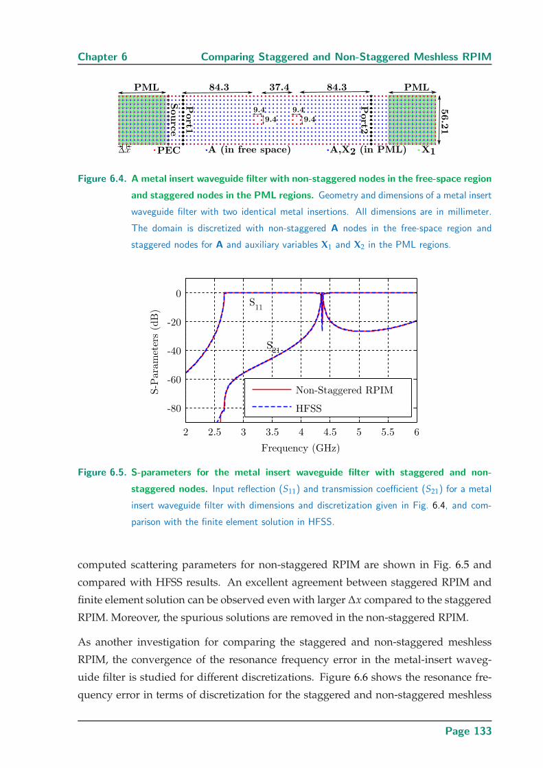
Chapter 6 Comparing Staggered and Non-Staggered Meshless RPIM
Figure 6.4. A metal insert waveguide filter with non-staggered nodes in the free-space region
and staggered nodes in the PML regions. Geometry and dimensions of a metal insert
waveguide filter with two identical metal insertions. All dimensions are in millimeter.
The domain is discretized with non-staggered A nodes in the free-space region and
staggered nodes for A and auxiliary variables X1 and X2 in the PML regions.
Figure 6.5. S-parameters for the metal insert waveguide filter with staggered and non-
staggered nodes. Input reflection (S11) and transmission coefficient (S21) for a metal
insert waveguide filter with dimensions and discretization given in Fig. 6.4, and com-
parison with the finite element solution in HFSS.
computed scattering parameters for non-staggered RPIM are shown in Fig. 6.5 and
compared with HFSS results. An excellent agreement between staggered RPIM and
finite element solution can be observed even with larger ∆x compared to the staggered
RPIM. Moreover, the spurious solutions are removed in the non-staggered RPIM.
As another investigation for comparing the staggered and non-staggered meshless
RPIM, the convergence of the resonance frequency error in the metal-insert waveg-
uide filter is studied for different discretizations. Figure 6.6 shows the resonance fre-
quency error in terms of discretization for the staggered and non-staggered meshless
Page 133
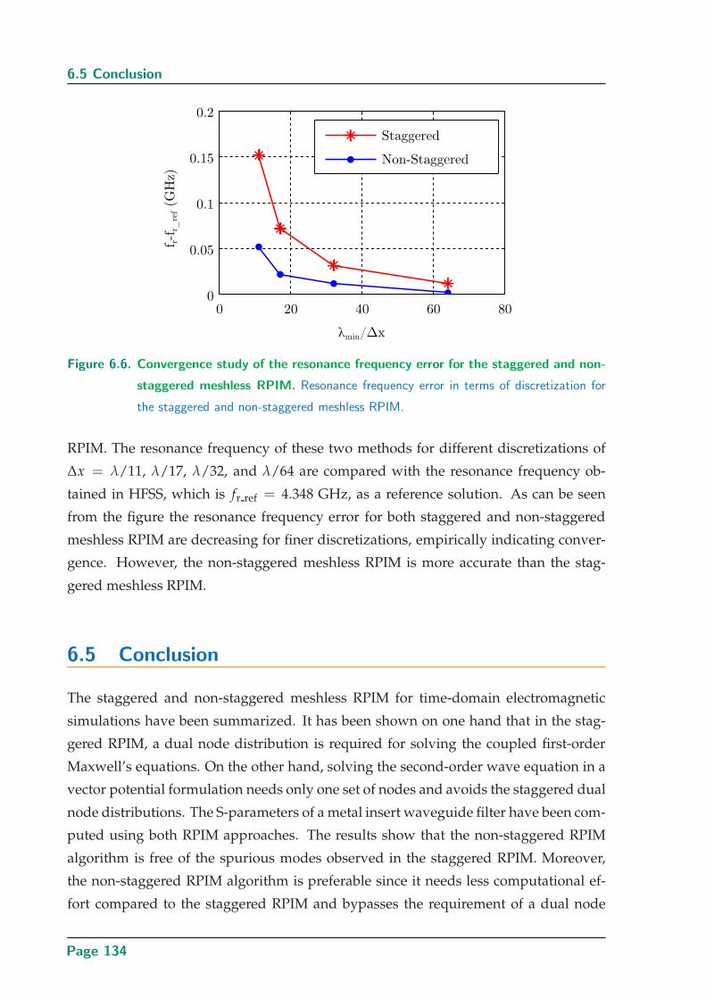
6.5 Conclusion
Figure 6.6. Convergence study of the resonance frequency error for the staggered and non-
staggered meshless RPIM. Resonance frequency error in terms of discretization for
the staggered and non-staggered meshless RPIM.
RPIM. The resonance frequency of these two methods for different discretizations of
∆x = λ/11, λ/17, λ/32, and λ/64 are compared with the resonance frequency ob-
tained in HFSS, which is fr ref = 4.348 GHz, as a reference solution. As can be seen
from the figure the resonance frequency error for both staggered and non-staggered
meshless RPIM are decreasing for finer discretizations, empirically indicating conver-
gence. However, the non-staggered meshless RPIM is more accurate than the stag-
gered meshless RPIM.
6.5 Conclusion
The staggered and non-staggered meshless RPIM for time-domain electromagnetic
simulations have been summarized. It has been shown on one hand that in the stag-
gered RPIM, a dual node distribution is required for solving the coupled first-order
Maxwell’s equations. On the other hand, solving the second-order wave equation in a
vector potential formulation needs only one set of nodes and avoids the staggered dual
node distributions. The S-parameters of a metal insert waveguide filter have been com-
puted using both RPIM approaches. The results show that the non-staggered RPIM
algorithm is free of the spurious modes observed in the staggered RPIM. Moreover,
the non-staggered RPIM algorithm is preferable since it needs less computational ef-
fort compared to the staggered RPIM and bypasses the requirement of a dual node
Page 134

Chapter 6 Comparing Staggered and Non-Staggered Meshless RPIM
distribution. Finally, a convergence study of the resonance frequency error in terms of
discretization has been conducted for the staggered and non-staggered meshless RPIM
demonstrating a faster convergence for the non-staggered meshless RPIM, with more
accurate results especially for a coarse discretization.
Page 135

Page 136
Chapter 7
Conclusion and FutureWork
THE research presented in this thesis has been described in two
major parts related to meshless Radial Point Interpolation Method
(RPIM): The first part of the thesis has placed the focus on the
staggered meshless RPIM. The second part of the thesis has investigated
the non-staggered meshless RPIM. This chapter concludes the thesis by
summarizing the original contributions, results and findings of the thesis.
The chapter also considers possible future research on staggered and non-
staggered meshless RPIM method.
Page 137
7.1 Part I: Staggered Meshless RPIM
Meshless methods were introduced to eliminate the costs and difficulties associated
with the generation of meshes in unstructured numerical methods. Compared to mesh-
based numerical techniques, the concept of meshless discretization suggests an ef-
ficient numerical treatment for complex geometries and multi-scale structures since
partial differential equations are solved on a cloud of arbitrarily distributed nodes.
Moreover, the straightforward addition of nodes to efficiently refine an initial coarse
node distribution can adaptively lead to more accurate results.
This chapter provides a summary of the original contributions and results of the two
major parts of the thesis along with a number of possible future directions of research
related to each part.
7.1 Part I: Staggered Meshless RPIM
The first major part of the thesis mainly encompasses Chapter 4 that focused on stag-
gered meshless Radial Point Interpolation Method (RPIM). This section gives a sum-
mary of the achieved results highlighting the original contributions described in the
last part of Chapter 3 and in Chapter 4. The section ends with suggestions for related
possible future work.
7.1.1 Summary of Original Contributions
• The Gaussian and Wendland basis functions have been compared for interpola-
tions in small local support domains. It has been shown that Gaussian basis func-
tions have a smaller interpolation error when applied on local support domain
with small sizes. As the size of support domain is increased the interpolation
error for the Wendland basis function becomes progressively smaller than the in-
terpolation error for the Gaussian basis function. This results show that truncated
Gaussian basis functions are a more appropriate choice compared to Wendland
basis functions in terms of accuracy when used in a time-domain meshless solver
where the small local support domains are preferable to achieve high computa-
tional efficiency [4].
Page 138
Chapter 7 Conclusion and Future Work
• The staggered meshless RPIM for the first-order Maxwell’s equations has been
implemented for 3D structures. In this method the space derivatives are dis-
cretized by RPIM approximations and the time derivatives are discretized by cen-
tral finite differences. The update equations have been provided for 3D staggered
meshless RPIM and have been validated though several numerical examples.
• In order to avoid spurious reflections caused by the truncation of the compu-
tational domains, absorbing boundaries are needed in numerical techniques to
absorb the energy of radiated waves. There are numerous techniques to simu-
late infinite space in numerical methods using absorbing boundary conditions.
Among them, the Perfectly Matched Layers (PMLs) are considered as one of the
most efficient techniques as they work for a wide range of incident angles and
frequencies. Therefore, variations of PML absorbing boundary conditions have
been developed for most volume-discretizing numerical methods in time and fre-
quency domain. In this thesis, the Uniaxial Perfectly Matched Layer (UPML) has
been adopted for 3D meshless RPIM and the long-time behavior of the UPML
has been studied. It has been shown that the UPML has long time instability that
can be avoided by introducing small losses in the UPML after most of the energy
in the computational domain has been absorbed in the UPML [10].
• The impact of different node distributions has been studied in a waveguide ex-
ample. A regular node distribution, a regular node distribution with 5% and 10%
random node displacement, and a cylindrical node distribution have been com-
pared at some observation points in terms of amplitude and phase of the electric
fields. The results have been shown to be very close to each other for different
node distributions, which demonstrates the robustness of the meshless RPIM for
different node distributions [11].
• Different node arrangements have been used to discretize a diplexer. This exam-
ple shows that meshless method can be used to discretize complex geometries
with in particular the ability to connect regular node arrangements with arbitrary
axes orientations [1].
• The scattering from a conducting sphere has been used for further validation of
the 3D RPIM method. In this example instead of solving the total electric field,
the scattered electric field is computed since the incident field is known. To this
end, the scattered field formulation has been described. Moreover, a near-field to
Page 139
7.2 Part II: Non-Staggered Meshless RPIM
far-field transformation has been implemented to compute the scattered electric
field in the far field. The simulation results have been compared to the theoretical
solutions demonstrating a very good agreement.
7.1.2 Future Work
# The face center of the Voronoi diagram has been chosen as dual node distribu-
tions in the 3D staggered meshless RPIM. Choosing Voronoi vertices as a dual
node distributions in 3D might results in chess-board propagation pattern. A
further study is required for finding the optimum dual node positions.
# One recurring issue of RPIM has been that small values of the shape parame-
ter result in accurate but unstable results, whereas the large values of the shape
parameter lead to less accurate but stable results. At present, a compromise be-
tween stability and accuracy has been chosen. However, additional studies are
required to automatically determine an optimum shape parameter to have stable
and accurate results.
# The Courant-Friedrich-Levy stability condition, which is based on the smallest
distance between nodes in the computational domain, has been used in this the-
sis. In the case of complex geometries with very different densities of nodes, the
local time-step scheme which was introduced in [160] for the Finite Volume Time
Domain (FVTD) method can be adapted for the meshless RPIM.
# Several numerical examples have been implemented and the results have been
compared with the solutions in HFSS or CST. More investigations are required to
improve the computational efficiency by optimizing the algorithm.
7.2 Part II: Non-Staggered Meshless RPIM
This section presents original contributions and possible future work related to the
second part of the thesis, which focused on the non-staggered meshless method.
7.2.1 Summary of Original Contributions
• Most time-domain meshless methods are solving Maxwell’s equations in a dual
node distribution with staggered nodes for the electric and magnetic fields. To
Page 140
Chapter 7 Conclusion and Future Work
bypass the requirement of a dual node distribution, a meshless magnetic vector
potential formulation has been introduced with only one set of nodes for solving
the wave equation. As additional advantage, this technique can reduce the nu-
merical effort since it solves three equations instead of six. This method has been
implemented first in a 2D parallel plate waveguide and a convergence study has
been performed, demonstrating convergence of the algorithm for different dis-
cretizations and also different numbers of neighbors included in the support do-
main. Moreover, the simulated scattering parameters of an iris filter simulated
using the proposed meshless magnetic vector potential method have been com-
pared to a mode-matching solution. A good agreement between simulation and
the mode-matching technique has provided further validation of the method.
To extend the considerations to all components, the magnetic vector potential
technique has been further validated for in-plane polarization. Finally, a 3D im-
plementation has also been shown for a square loop antenna and the radiation
pattern has been compared with the analytical solutions [2].
• The formulation for the first and second-order meshless RPIM have been intro-
duced and these two methods have been compared. Solving the first order Max-
well’s equations requires a dual staggered node distribution in space, whereas
solving the second-order wave equation needs only a single set of nodes but
can exploit the ability of meshless methods to accurately estimate second-order
derivatives. Moreover, in the first-order discretization to avoid unphysical solu-
tions of the fields, the divergence property of the fields needs to be considered. In
contrast, in a formulation based on a second-order vector potential method the
divergence property of the fields are automatically enforced [7].
• Implementing magnetic vector potential needs a single set of nodes for A. On
the other hand, to implement PML with a stretched coordinate approach, a stag-
gered node distributions for A and auxiliary variables is required. To avoid hav-
ing staggered nodes in the whole computational domain, a hybrid algorithm has
been introduced to implement staggered PML in a non-staggered meshless RPIM
formulation. In this case staggered node distribution is limited to the PML region
where a structured node distribution is generally in use and dual node genera-
tion is straightforward [6].
• In the last part, staggered and non-staggered meshless RPIM have been com-
pared. The results from a metal insert waveguide filter indicate that the solution
Page 141
7.2 Part II: Non-Staggered Meshless RPIM
of the staggered meshless RPIM has spurious solutions. However, non-staggered
meshless RPIM not only does not require a dual node distribution but also avoids
the spurious modes in the solutions. This clearly demonstrates the superiority of
the non-staggered vector potential algorithm [8].
7.2.2 Future Work
# The magnetic vector potential technique has been introduced and validated for
several examples in 2D. This method has also been validated for the preliminary
example of a square loop antenna in 3D. However, the applicable range of the 3D
magnetic vector potential needs to be extended further.
# One of the main advantage of the magnetic vector potential method is to bypass
the requirement for the dual node distribution. Moreover, the spurious solutions
can be avoided using this technique. However, implementing derivative bound-
ary conditions is not straightforward in this method. There are some techniques
to implement the derivative boundary conditions, e.g., using dummy nodes or
using Hermite interpolation. In this thesis dummy nodes have been used to ap-
ply the derivative boundary conditions. Using other techniques, such as Hermite
interpolation, to apply Neumann boundary conditions can be seen as another fu-
ture work.
# The stretched coordinate system has been used to implement the PML in the non-
staggered meshless RPIM. This method needs staggered nodes for the auxiliary
variables and the magnetic vector potential. Further research to use a different
approach that can be implemented without introducing staggered auxiliary vari-
ables seems highly promising.
# In a staggered meshless RPIM, using divergence-free vector basis functions can
avoid spurious solutions. In a non-staggered meshless RPIM the magnetic vector
potential technique avoids unphysical solutions. Further research is required to
find a mathematical relation between divergence-free vector basis functions and
the basis functions in the magnetic vector potential technique.
# Parallelization of the algorithm can be considered as another future work to
speed up the algorithm.
Page 142
Chapter 7 Conclusion and Future Work
In conclusion, meshless methods can be seen as a type of generalized FDTD with flex-
ible node distributions. The results in this thesis emphasize the attractive features of
the meshless RPIM to discretize the complex geometries and to obtain highly accurate
results.
Page 143

Page 144
Appendix A
Theoretical Solution for theScattering of
Electromagnetic Wavesfrom a Conducting Sphere
In this section, the theoretical solution (Mie solution) for the scattering from a conduct-
ing sphere in the far field is summarized. The scattered electric field can be expressed
as follows [144]
Es =∞
∑n=1
En(jan Ne1n − bnMo1n), (A.1)
where En is
En = jn 2n + 1
n(n + 1). (A.2)
Also, Mo1n and Ne1n are the spherical vector harmonics (which will be explained later),
and the scattering coefficients an and bn are combination of Hankel and Bessel func-
tions [144]. Using boundary condition for the conducting sphere, the coefficients an
and bn can be found as follows [161]
an = − [xjn(x)]′
[xhn(x)]′ , (A.3)
bn = − jn(x)
hn(x), (A.4)
where x = kr at the observation point r, k = 2π/λ, jn(x) is the spherical Bessel function
of first kind, and hn(x) is the spherical Hankel function of first kind. The spherical
Bessel functions of first and second kind are as follows
jn(x) =
√π
2xJn+0.5(x), (A.5a)
yn(x) =
√π
2xYn+0.5(x), (A.5b)
Page 145
where Jn+0.5(x) and Yn+0.5(x) are the Bessel functions of first and second kind that can
be computed using the commands “besselj (n + 0.5, x)” and “bessely (n + 0.5, x)” in
Matlab. Also, the spherical Hankel function of the first kind in (A.3) and (A.4) can be
written in terms of the spherical Bessel functions as follows
hn(x) = jn(x) + jyn(x), (A.6)
and
[xjn(x)]′= xjn−1(x)− njn(x), (A.7a)
[xhn(x)]′= xhn−1(x)− nhn(x). (A.7b)
In equation (A.1), Mo1n and Ne1n are as follows
Ne1n =hn(x)
xcos φn(n + 1) sin θπn er + cos φτn
[xhn(x)]′
xeθ − sin φπn
[xhn(x)]′
xeφ,
(A.8a)
Mo1n = cos φπnhn(x)eθ − sin φτnhn(x)eφ. (A.8b)
In above equations πn and τn are defined as
πn =2n − 1
n − 1µπn−1 −
n
n − 1πn−2, (A.9a)
τn = nµπn − (n + 1)πn−1, (A.9b)
where µ = cos θ, and the two first terms for πn and τn are given by
π1 = 1, π2 = 3 cos(θ), (A.10a)
τ1 = cos(θ), τ2 = 3 cos(2θ). (A.10b)
The infinite series in (A.1) can be approximated by considering nmax terms. The pro-
posed number for nmax in [144] is given by
nmax = x + 4x13 + 2. (A.11)
The value of nmax for r = λ/2 is 11. Finally, the scattered electric field with the trun-
cated series can be approximated as follows
Esθ ≃ − ejkr
−jkrcos φS2(cos θ), (A.12a)
Esφ ≃ − ejkr
−jkrsin φS1(cos θ), (A.12b)
Page 146

Appendix A Scattering from a Conducting Sphere: Theoretical Solution
where
S1 =nmax
∑n=1
2n + 1
n(n + 1)(anπn + bnτn), (A.13a)
S2 =nmax
∑n=1
2n + 1
n(n + 1)(anτn + bnπn). (A.13b)
Page 147

Page 148
Appendix B
Useful Identities inCylindrical Coordinate
System
Some useful identities in cylindrical coordinate system (or polar coordinate system by
neglecting z-component) are summarized in this appendix:
∇ f =∂ f
∂ρρ +
1
ρ
∂ f
∂ΦΦ +
∂ f
∂zz (B.1)
∇ · A =1
ρ
∂(ρAρ)
∂ρ+
1
ρ
∂AΦ
∂Φ+
∂Az
∂z(B.2)
∇× A = (1
ρ
∂Az
∂Φ− ∂AΦ
∂z)ρ + (
∂Aρ
∂z− ∂Az
∂Φ)Φ +
1
ρ(
∂(ρAφ)
∂ρ− ∂Aρ
∂Φ)z (B.3)
∇2A =
∂2 Aρ
∂ρ2 + 1ρ2
∂2 Aρ
∂Φ2 +∂2 Aρ
∂z2 + 1ρ
∂Aρ
∂ρ − 2ρ2
∂AΦ
∂Φ− Aρ
ρ2
∂2 AΦ
∂ρ2 + 1ρ2
∂2 AΦ
∂Φ2 + ∂2 AΦ
∂z2 + 1ρ
∂AΦ
∂ρ + 2ρ2
∂Aρ
∂Φ− AΦ
ρ2
∂2 Az
∂ρ2 + 1ρ2
∂2 Az
∂Φ2 + ∂2 Az
∂z2 + 1ρ
∂Az∂ρ
(B.4)
Page 149

Page 150
Appendix C
StaggeredBackward-Differentiation
Time Integrators
In order to increase the stability and accuracy in differentiation methods, staggered
grids in time and space can be used. In [157] some staggered ordinary differential
equations including staggered backward-differentiation time integrators (BDSp) have
been introduced, where (p+1) is the order of the normalized local truncation error. The
explicit Taylor equation for BDS3 is defined as follows
y(t + ∆t) =21
23y(t) +
2
23y(t − ∆t)− 1
23y(t − 2∆t) +
24∆t
23y′(t +
∆t
2) + O(∆t4), (C.1)
or
y′(t +∆t
2) ≃ 23
24∆t
(y(t + ∆t)− 21
23y(t)− 2
23y(t − ∆t) +
1
23y(t − 2∆t)
). (C.2)
In this section, the discretization of the wave equation for magnetic vector potential
using BDS3 is introduced. The wave equation is repeated here for convenience as
∇2A − µǫ∂
∂t
(∂A
∂t
)= −µJ. (C.3)
An auxiliary variable DA is then defined for discretization as
DA =∂A
∂t. (C.4)
Therefore, equation (C.3) using the auxiliary variable DA at time step n is discretized
as follows (∂2An
∂x2+
∂2An
∂y2
)− µǫ
∂DAn
∂t= −µJn. (C.5)
Page 151
After some manipulations, (C.5) is written as
1
µǫ
(∂2An
∂x2+
∂2An
∂y2
)+
Jn
ǫ=
∂DAn
∂t. (C.6)
Using RPIM and BDS3 to discretize the space and time derivatives in (C.3) gives
1
µǫ
(∂2φ(x)
∂x2An +
∂2φ(x)
∂y2An
)+
Jn
ǫ=
23
24∆t
(DAn+ 1
2 − 21
23DAn− 1
2 − 3
23DAn− 3
2 +1
23DAn− 5
2
),
(C.7)
which results in the following update equation for the axillary variable DA
DAn+ 12 =
24∆t
23
1
µǫ(
∂2An
∂x2+
∂2An
∂y2) +
24∆t
23
Jn
ǫ+
21
23DAn− 1
2 +3
23DAn− 3
2 − 1
23DAn− 5
2 .
(C.8)
Also, using the BDS3 to discretize (C.4) gives
DAn+ 12 =
∂An+ 12
∂t=
23
24∆t(An+1 − 21
23An − 3
23An−1 +
1
23An−2), (C.9)
which gives the following update equation for A after some manipulations
An+1 =24∆t
23DAn+ 1
2 +21
23An +
3
23An−1 − 1
23An−2. (C.10)
This update equation is an explicit equation in time that depends on the magnetic
vector potential A and DA from the past time steps. Note that DA can be updated
based on update equation in (C.8).
Page 152
Bibliography
[1] C. Fumeaux, T. Kaufmann, Z. Shaterian, D. Baumann, and M. Klemm, Conformal and Multi-Scale
Time-Domain Methods: From Unstructured Meshes to Meshless Discretisations. Chapter 6 in Compu-
tational Electromagnetics Retrospective and Outlook: In Honor of Wolfgang J. R. Hoefer, Springer,
2015.
[2] Z. Shaterian, T. Kaufmann, and C. Fumeaux, “Time-domain vector potential technique for the
meshless radial point interpolation method,” International Journal for Numerical Methods in Engi-
neering, 2015 (in print).
[3] A. K. Horestani, J. Naqui, Z. Shaterian, D. Abbott, C. Fumeaux, and F. Martın, “Two-dimensional
alignment and displacement sensor based on movable broadside-coupled split ring resonators,”
Sensors and Actuators A: Physical, vol. 210, pp. 18–24, 2014.
[4] Z. Shaterian, T. Kaufmann, and C. Fumeaux, “On the choice of basis functions for the meshless
radial point interpolation method with small local support domains,” in International Conference
on Computational Electromagnetics (iCCEM), Hong Kong, 2-5 February 2015.
[5] Z. Shaterian, A. K. Horestani, and C. Fumeaux, “Rotation sensing based on the symmetry prop-
erties of an open-ended microstrip line loaded with a split ring resonator,” in German Microwave
Conference (GeMiC), Nuremberg, Germany, 16-18 March 2015.
[6] Z. Shaterian, T. Kaufmann, and C. Fumeaux, “Hybrid staggered perfectly matched layers in non-
staggered meshless time-domain vector potential technique,” in International Workshop on Antenna
Technology (iWAT), Sydney, Australia, 4-6 March 2014, pp. 408–411.
[7] ——, “First- and second-order meshless radial point interpolation methods in electromagnetics,”
in 1st Australian Microwave Symposium (AMS), Melbourne, Australia, 26-27 June 2014.
[8] ——, “On the staggered and non-staggered time-domain meshless radial point interpolation
method,” in 17th International Symposium on ElectroMagnetic Compatibility (CEM), Clermont-
Ferrand, France, 30 June- 3 July 2014.
[9] Z. Shaterian, A. K. Horestani, and C. Fumeaux, “Metamaterial-inspired displacement sensor with
high dynamic range,” in International Conference on Metamaterials, Photonic Crystals and Plasmonics
(META), United Arab Emirates, 2013.
[10] Z. Shaterian, T. Kaufmann, and C. Fumeaux, “On the late-time instability of perfectly matched
layers in the meshless radial point interpolation method,” in Asia-Pacific Microwave Conference
(APMC) Proceedings, Seoul, Korea, 5-8 November 2013, pp. 845–847.
[11] ——, “Impact of different node distributions on the meshless radial point interpolation method in
time-domain electromagnetic simulations,” in Asia-Pacific Microwave Conference (APMC), Kaohsi-
ung, Taiwan, 4-7 December 2012.
Page 153
Bibliography
[12] A. K. Horestani, Z. Shaterian, T. Kaufmann, and C. Fumeaux, “Single and dual band-notched
ultra-wideband antenna based on dumbbell-shaped defects and complementary split ring res-
onators,” in German Microwave Conference (GeMiC), Nuremberg, Germany, 16-18 March 2015.
[13] A. Horestani, Z. Shaterian, and C. Fumeaux, “Application of metamaterial-inspired resonators
in compact microwave displacement sensors,” in Australian Microwave Symposium (AMS), Mel-
bourne, Australia, 26-27 June 2014.
[14] A. K. Horestani, Z. Shaterian, S. Al-Sarawi, D. Abbott, and C. Fumeaux, “Miniaturized bandpass
filter with wide stopband using complementary spiral resonator,” in Proc. Asia-Pacific Microwave
Conference (APMC), Kaohsiung, Taiwan, 4-7 December 2012, pp. 550–552.
[15] A. Horestani, Z. Shaterian, S. Al-Sarawi, and D. Abbott, “High quality factor mm-wave coplanar
strip resonator based on split ring resonators,” in 36th International Conference on Infrared, Millime-
ter and Terahertz Waves (IRMMW-THz), Houston, 2-7 October 2011.
[16] A. K. Horestani, Z. Shaterian, W. Withayachumnankul, C. Fumeaux, S. Al-Sarawi, and D. Ab-
bott, “Compact wideband filter element-based on complementary split-ring resonators,” in Smart
Nano-Micro Materials and Devices. International Society for Optics and Photonics, 2011.
[17] Z. Shaterian and M. Ardebilipour, “Direct sequence and time hopping ultra wideband over
IEEE.802.15.3a channel model,” in 16th International Conference on Software, Telecommunications and
Computer Networks (SoftCOM), 2008, pp. 90–94.
[18] M. N. Sadiku, Numerical Techniques in Electromagnetics. CRC press, 2000.
[19] S. Lai, B. Wang, and Y. Duan, “Meshless radial basis function method for transient electromagnetic
computations,” IEEE Transactions on Magnetics, vol. 44, no. 10, pp. 2288–2295, 2008.
[20] T. Kaufmann, C. Fumeaux, and R. Vahldieck, “The meshless radial point interpolation method for
time-domain electromagnetics,” in IEEE MTT-S International Microwave Symposium Digest, 2008,
pp. 61–64.
[21] Y. Yu and Z. Chen, “A 3-D radial point interpolation method for meshless time-domain model-
ing,” IEEE Transactions on Microwave Theory and Techniques, vol. 57, no. 8, pp. 2015–2020, 2009.
[22] T. Kaufmann, Y. Yu, C. Engstrom, Z. Chen, and C. Fumeaux, “Recent developments of the mesh-
less radial point interpolation method for time-domain electromagnetics,” International Journal of
Numerical Modelling: Electronic Networks, Devices and Fields, pp. 468–489, 2012.
[23] N. Sukumar, B. Moran, A. Yu Semenov, and V. Belikov, “Natural neighbour Galerkin methods,”
International Journal for Numerical Methods in Engineering, vol. 50, no. 1, pp. 1–27, 2001.
[24] T. Kaufmann, C. Engstrom, C. Fumeaux, and R. Vahldieck, “Eigenvalue analysis and longtime sta-
bility of resonant structures for the meshless radial point interpolation method in time domain,”
IEEE Transactions on Microwave Theory and Techniques, vol. 58, no. 12, pp. 3399–3408, 2010.
[25] S. Yang, Z. Chen, Y. Yu, and S. Ponomarenko, “A divergence-free meshless method based on
the vector basis function for transient electromagnetic analysis,” IEEE Transactions on Microwave
Theory and Techniques, vol. 62, no. 7, pp. 1409–1416, 2014.
Page 154
Bibliography
[26] H. Razmjoo, M. Movahhedi, and A. Hakimi, “Electromagnetic time domain modeling using an
improved meshless method,” in IEEE MTT-S International Microwave Symposium Digest, 2011, pp.
1–4.
[27] N. Georgieva and E. Yamashita, “Time-domain vector-potential analysis of transmission-line
problems,” IEEE Transactions on Microwave Theory and Techniques, vol. 46, no. 4, pp. 404–410, 1998.
[28] K. Yee, “Numerical solution of initial boundary value problems involving Maxwell’s equations in
isotropic media,” IEEE Transactions on Antennas and Propagation, vol. 14, no. 3, pp. 302–307, 1966.
[29] A. Taflove and S. Hagness, Computational Electrodynamics: The Finite-Difference Time-Domain
Method. Artech House Boston, 2005.
[30] D. B. Davidson, Computational Electromagnetics for RF and Microwave Engineering. Cambridge
University Press, 2005.
[31] Y. Nomura and T. Hatta, “The theory of a linear antenna,” Technology Reports, Tohoku University,
vol. 17, 1952.
[32] B. Storm, “Investigation into modern aerial theory and a new solution of Hallen’s integral equa-
tion for a cylindrical aerial,” Ph.D. dissertation, Imperial College, London, 1953.
[33] L. Kantorovich and V. Krylov, “Approximate methods of higher analysis,” Bull. Amer. Math. Soc.,
1960.
[34] L. Kantorovich and G. Akilov, “Functional analysis in normed spaces,” 1959.
[35] R. F. Harrington, “Matrix methods for field problems,” Proceedings of the IEEE, vol. 55, no. 2, pp.
136–149, 1967.
[36] ——, Field Computation by Moment Methods. New York: Macmillan, 1968.
[37] R. Courant, “Variational methods for the solution of problems of equilibrium and vibrations,”
Bulletin of American mathematical Society, pp. 1–23, 1943.
[38] P. Silvester, “Finite element solution of homogeneous waveguide problems,” Alta Frequenza,
vol. 38, pp. 313–317, 1969.
[39] R. Coccioli, T. Itoh, G. Pelosi, and P. Silvester, “Finite-element methods in microwaves: A selected
bibliography,” IEEE Antennas and Propagation Magazine, vol. 38, no. 6, pp. 34–48, 1996.
[40] G. Pelosi, R. Coccioli, and S. Selleri, Quick Finite Elements for Electromagnetic Waves. Artech House
Publishers, 2009.
[41] J. Jin, The Finite Element Method in Electromagnetics. New York: JohnWiley & Sons, 2002.
[42] B. Beillard, J. Andrieu, Y. Chevalier, and B. Jecko, “Electromagnetic “zoom” in FDTD,” in 26th
European Microwave Conference, 1996, pp. 435–439.
[43] A. Rennings, J. Mosig, C. Caloz, D. Erni, and P. Waldow, “Equivalent circuit (EC) FDTD method
for the modeling of surface plasmon based couplers,” Journal of Computational and Theoretical
Nanoscience, vol. 5, no. 4, pp. 690–703, 2008.
Page 155
Bibliography
[44] T. Kaufmann, C. Engstrom, and C. Fumeaux, “Residual-based adaptive refinement for mesh-
less eigenvalue solvers,” in International Conference on Electromagnetics in Advanced Applications
(ICEAA), Sydney, 2010, pp. 244–247.
[45] T. Belytschko, Y. Krongauz, D. Organ, M. Fleming, and P. Krysl, “Meshless methods: an overview
and recent developments,” Computer methods in applied mechanics and engineering, vol. 139, no. 1,
pp. 3–47, 1996.
[46] R. A. Gingold and J. J. Monaghan, “Smoothed particle hydrodynamics: theory and application to
non-spherical stars,” Monthly notices of the royal astronomical society, vol. 181, no. 3, pp. 375–389,
1977.
[47] L. B. Lucy, “A numerical approach to the testing of the fission hypothesis,” The astronomical journal,
vol. 82, pp. 1013–1024, 1977.
[48] J. J. Monaghan, “Why particle methods work,” SIAM Journal on Scientific and Statistical Computing,
vol. 3, no. 4, pp. 422–433, 1982.
[49] ——, “An introduction to SPH,” Computer physics communications, vol. 48, no. 1, pp. 89–96, 1988.
[50] ——, “Smoothed particle hydrodynamics,” Annual review of astronomy and astrophysics, vol. 30, pp.
543–574, 1992.
[51] B. Nayroles, G. Touzot, and P. Villon, “Generalizing the finite element method: diffuse approxi-
mation and diffuse elements,” Computational mechanics, vol. 10, no. 5, pp. 307–318, 1992.
[52] P. Breitkopf, A. Rassineux, J. Savignat, and P. Villon, “Integration constraint in diffuse element
method,” Computer methods in applied mechanics and engineering, vol. 193, no. 12-14, pp. 1203–1220,
2004.
[53] Y. Marechal, J. Coulomb, G. Meunier, and G. Touzot, “Use of the diffuse element method for
electromagnetic field computation,” IEEE Transactions on Magnetics, vol. 29, no. 2, pp. 1475–1478,
1993.
[54] S. Qian and J. Weiss, “Wavelets and the numerical solution of partial differential equations,” Jour-
nal of Computational Physics, vol. 106, no. 1, pp. 155–175, 1993.
[55] T. Belytschko, Y. Y. Lu, and L. Gu, “Element-free Galerkin methods,” International journal for nu-
merical methods in engineering, vol. 37, no. 2, pp. 229–256, 1994.
[56] Y. Lu, T. Belytschko, and L. Gu, “A new implementation of the element free Galerkin method,”
Computer Methods in Applied Mechanics and Engineering, vol. 113, no. 3-4, pp. 397–414, 1994.
[57] D. Sulsky, S.-J. Zhou, and H. L. Schreyer, “Application of a particle-in-cell method to solid me-
chanics,” Computer Physics Communications, vol. 87, no. 1, pp. 236–252, 1995.
[58] W. K. Liu, S. Jun, and Y. F. Zhang, “Reproducing kernel particle methods,” International Journal for
Numerical Methods in Fluids, vol. 20, no. 8-9, pp. 1081–1106, 1995.
[59] W. K. Liu, R. A. Uras, and Y. Chen, “Enrichment of the finite element method with the reproducing
kernel particle method,” Journal of Applied Mechanics, vol. 64, no. 4, pp. 861–870, 1997.
Page 156
Bibliography
[60] I. Babuska and J. M. Melenk, “The partition of unity finite element method,” DTIC Document,
Tech. Rep., 1995.
[61] J. M. Melenk and I. Babuska, “The partition of unity finite element method: basic theory and
applications,” Computer methods in applied mechanics and engineering, vol. 139, no. 1, pp. 289–314,
1996.
[62] C. A. Duarte and J. T. Oden, “Hp clouds-an hp meshless method,” Numerical methods for partial
differential equations, vol. 12, no. 6, pp. 673–706, 1996.
[63] ——, “An h-p adaptive method using clouds,” Computer methods in applied mechanics and engineer-
ing, vol. 139, no. 1, pp. 237–262, 1996.
[64] E. Onate, S. Idelsohn, O. Zienkiewicz, and R. Taylor, “A finite point method in computational
mechanics. applications to convective transport and fluid flow,” International journal for numerical
methods in engineering, vol. 39, no. 22, pp. 3839–3866, 1996.
[65] E. Onate, S. Idelsohn, O. Zienkiewicz, R. Taylor, and C. Sacco, “A stabilized finite point method
for analysis of fluid mechanics problems,” Computer Methods in Applied Mechanics and Engineering,
vol. 139, no. 1, pp. 315–346, 1996.
[66] G. Yagawa and T. Furukawa, “Recent developments of free mesh method,” International Journal
for Numerical Methods in Engineering, vol. 47, no. 8, pp. 1419–1443, 2000.
[67] T. Zhu, “A new meshless regular local boundary integral equation (MRLBIE) approach,” Interna-
tional Journal for Numerical Methods in Engineering, vol. 46, no. 8, pp. 1237–1252, 1999.
[68] S. Atluri and T. Zhu, “New concepts in meshless methods,” International Journal for Numerical
Methods in Engineering, vol. 47, no. 1-3, pp. 537–556, 2000.
[69] W. K. Liu, Y. Chen, R. A. Uras, and C. T. Chang, “Generalized multiple scale reproducing kernel
particle methods,” Computer Methods in Applied Mechanics and Engineering, vol. 139, no. 1, pp. 91–
157, 1996.
[70] W. K. Liu, Y. Chen, C. Chang, and T. Belytschko, “Advances in multiple scale kernel particle
methods,” Computational Mechanics, vol. 18, no. 2, pp. 73–111, 1996.
[71] W.-K. Liu, S. Li, and T. Belytschko, “Moving least-square reproducing kernel methods (I) method-
ology and convergence,” Computer Methods in Applied Mechanics and Engineering, vol. 143, no. 1,
pp. 113–154, 1997.
[72] W. K. Liu, S. Hao, T. Belytschko, S. Li, and C. T. Chang, “Multi-scale methods,” International Journal
for Numerical Methods in Engineering, vol. 47, no. 7, pp. 1343–1361, 2000.
[73] G.-R. Liu and Y.-T. Gu, An Introduction to Meshfree Methods and Their Programming. Springer, 2005.
[74] S. Atluri and T. Zhu, “A new meshless local Petrov-Galerkin (MLPG) approach in computational
mechanics,” Computational mechanics, vol. 22, no. 2, pp. 117–127, 1998.
[75] C. Durate and J. Oden, “Hp clouds-a meshless method to solve boundary-value problems,” Texas
Institute for Computational and Applied Mathematics Report, pp. 95–06, 1995.
Page 157
Bibliography
[76] N. Perrone and R. Kao, “A general finite difference method for arbitrary meshes,” Computers &
Structures, vol. 5, no. 1, pp. 45–57, 1975.
[77] V. Pavlin and N. Perrone, “Finite difference energy techniques for arbitrary meshes applied to
linear plate problems,” International Journal for Numerical Methods in Engineering, vol. 14, no. 5, pp.
647–664, 1979.
[78] T. Liszka and J. Orkisz, “Finite difference method at arbitrary irregular meshes in non-linear prob-
lems of applied mechanics,” in Int. Conf. on Structural Mech., San Francisco, USA, 1977.
[79] ——, “The finite difference method at arbitrary irregular grids and its application in applied me-
chanics,” Computers & Structures, vol. 11, no. 1, pp. 83–95, 1980.
[80] J. Krok and J. Orkisz, “A unified approach to the FE and generalized variational FD methods
in nonlinear mechanics, concepts and numerical approach,” in Discretization methods in structural
mechanics. Springer, 1990, pp. 353–362.
[81] E. J. Kansa, “Multiquadrics–A scattered data approximation scheme with applications to compu-
tational fluid-dynamics–II solutions to parabolic, hyperbolic and elliptic partial differential equa-
tions,” Computers & mathematics with applications, vol. 19, no. 8, pp. 147–161, 1990.
[82] W. Zongmin, “Hermite-birkhoff interpolation of scattered data by radial basis functions,” Approx-
imation Theory and its Applications, vol. 8, no. 2, pp. 1–10, 1992.
[83] X. Zhang, K. Z. Song, M. W. Lu, and X. Liu, “Meshless methods based on collocation with radial
basis functions,” Computational mechanics, vol. 26, no. 4, pp. 333–343, 2000.
[84] X. Liu, G. Liu, K. Tai, and K. Lam, “Radial point interpolation collocation method (RPICM) for
the solution of nonlinear poisson problems,” Computational Mechanics, vol. 36, no. 4, pp. 298–306,
2005.
[85] J. Wang and G. Liu, “A point interpolation meshless method based on radial basis functions,”
International Journal for Numerical Methods in Engineering, vol. 54, no. 11, pp. 1623–1648, 2002.
[86] X. Liu, “Radial point collocation method (RPCM) for solving convection-diffusion problems,”
Journal of Zhejiang University SCIENCE A, vol. 7, no. 6, pp. 1061–1067, 2006.
[87] E. Onate, “Derivation of stabilized equations for numerical solution of advective-diffusive trans-
port and fluid flow problems,” Computer Methods in Applied Mechanics and Engineering, vol. 151,
no. 1, pp. 233–265, 1998.
[88] E. Onate, F. Perazzo, and J. Miquel, “A finite point method for elasticity problems,” Computers &
Structures, vol. 79, no. 22, pp. 2151–2163, 2001.
[89] G. Liu and Y. Gu, “A meshfree method: meshfree weak–strong (MWS) form method, for 2-D
solids,” Computational Mechanics, vol. 33, no. 1, pp. 2–14, 2003.
[90] G.-R. Liu, Meshfree Methods: Moving Beyond the Finite Element Method. CRC press, 2010.
[91] X. Liu, B.-Z. Wang, and S. Lai, “Element-free Galerkin method in electromagnetic scattering field
computation,” Journal of Electromagnetic Waves and Applications, vol. 21, no. 14, pp. 1915–1923, 2007.
Page 158
Bibliography
[92] G. Ala, E. Francomano, A. Tortorici, E. Toscano, and F. Viola, “Corrective meshless particle formu-
lations for time domain Maxwell’s equations,” Journal of Computational and Applied Mathematics,
vol. 210, no. 1, pp. 34–46, 2007.
[93] D. Soares Jr, “Numerical modelling of electromagnetic wave propagation by meshless local
Petrov-Galerkin formulations,” Computer Modeling in Engineering and Sciences (CMES), vol. 19,
no. 2, p. 97, 2009.
[94] G.-R. Liu and M. B. Liu, Smoothed Particle Hydrodynamics: A Meshfree Particle Method. World
Scientific, 2003.
[95] M. Liu and G. Liu, “Smoothed particle hydrodynamics (SPH): an overview and recent develop-
ments,” Archives of computational methods in engineering, vol. 17, no. 1, pp. 25–76, 2010.
[96] C. Zhou, G. Liu, and K. Lou, “Three-dimensional penetration simulation using smoothed particle
hydrodynamics,” International Journal of Computational Methods, vol. 4, no. 04, pp. 671–691, 2007.
[97] J.-S. Chen, C. Pan, C.-T. Wu, and W. K. Liu, “Reproducing kernel particle methods for large defor-
mation analysis of non-linear structures,” Computer Methods in Applied Mechanics and Engineering,
vol. 139, no. 1, pp. 195–227, 1996.
[98] W. K. Liu, “Multiresolution reproducing kernel particle methods in acoustics,” The Journal of the
Acoustical Society of America, vol. 100, no. 4, pp. 2685–2685, 1996.
[99] R. Uras, C.-T. Chang, Y. Chen, and W. Liu, “Multiresolution reproducing kernel particle methods
in acoustics,” Journal of Computational Acoustics, vol. 5, no. 01, pp. 71–94, 1997.
[100] R. MacNeal, “An asymmetrical finite difference network,” Quart. Appl. Math, vol. 11, no. 3, pp.
295–310, 1953.
[101] L. Collatz, Numerische Behandlung von Differentialgleichungen. Springer Verlag, 1955.
[102] D. Shepard, “A two-dimensional interpolation function for irregularly-spaced data,” in Proceed-
ings of the 1968 23rd ACM national conference. ACM, 1968, pp. 517–524.
[103] X. Zheng, W.-Y. Duan, and Q.-W. Ma, “Comparison of improved meshless interpolation schemes
for SPH method and accuracy analysis,” Journal of Marine Science and Application, vol. 9, no. 3, pp.
223–230, 2010.
[104] G. Liu and Y. Gu, “A point interpolation method for two-dimensional solids,” International Journal
for Numerical Methods in Engineering, vol. 50, no. 4, pp. 937–951, 2001.
[105] J. Wang, G. Liu, and Y. Wu, “A point interpolation method for simulating dissipation process of
consolidation,” Computer Methods in Applied Mechanics and Engineering, vol. 190, no. 45, pp. 5907–
5922, 2001.
[106] M. D. Buhmann, Radial Basis Functions: Theory and Implementations. Cambridge university press,
2003, vol. 5.
[107] R. Franke, “Scattered data interpolation: Tests of some methods,” Mathematics of computation,
vol. 38, no. 157, pp. 181–200, 1982.
Page 159
Bibliography
[108] R. L. Hardy, “Theory and applications of the multiquadric-biharmonic method 20 years of discov-
ery 1968–1988,” Computers & Mathematics with Applications, vol. 19, no. 8, pp. 163–208, 1990.
[109] M. Fornefett, K. Rohr, and H. S. Stiehl, “Radial basis functions with compact support for elastic
registration of medical images,” Image and Vision Computing, vol. 19, no. 1, pp. 87–96, 2001.
[110] E. J. Kansa, “Multiquadrics–A scattered data approximation scheme with applications to compu-
tational fluid-dynamics–I surface approximations and partial derivative estimates,” Computers &
Mathematics with applications, vol. 19, no. 8, pp. 127–145, 1990.
[111] G. E. Fasshauer, “Solving partial differential equations by collocation with radial basis functions,”
in Proceedings of Chamonix. Vanderbilt University Press, 1997, pp. 131–138.
[112] C. Franke and R. Schaback, “Solving partial differential equations by collocation using radial basis
functions,” Applied Mathematics and Computation, vol. 93, no. 1, pp. 73–82, 1998.
[113] B. Jumarhon, S. Amini, and K. Chen, “The Hermite collocation method using radial basis func-
tions,” Engineering analysis with boundary elements, vol. 24, no. 7, pp. 607–611, 2000.
[114] Y. Hon and R. Schaback, “On unsymmetric collocation by radial basis functions,” Applied Mathe-
matics and Computation, vol. 119, no. 2, pp. 177–186, 2001.
[115] Y. Wu and C. Shu, “Development of RBF-DQ method for derivative approximation and its appli-
cation to simulate natural convection in concentric annuli,” Computational Mechanics, vol. 29, no. 6,
pp. 477–485, 2002.
[116] E. Larsson and B. Fornberg, “A numerical study of some radial basis function based solution
methods for elliptic PDEs,” Computers & Mathematics with Applications, vol. 46, no. 5, pp. 891–902,
2003.
[117] R. B. Platte and T. A. Driscoll, “Computing eigenmodes of elliptic operators using radial basis
functions,” Computers & Mathematics with Applications, vol. 48, no. 3, pp. 561–576, 2004.
[118] M. Tatari and M. Dehghan, “On the solution of the non-local parabolic partial differential equa-
tions via radial basis functions,” Applied Mathematical Modelling, vol. 33, no. 3, pp. 1729–1738, 2009.
[119] K. Parand, S. Abbasbandy, S. Kazem, and J. Rad, “A novel application of radial basis functions for
solving a model of first-order integro-ordinary differential equation,” Communications in Nonlinear
Science and Numerical Simulation, vol. 16, no. 11, pp. 4250–4258, 2011.
[120] J. L. Bentley, “Multidimensional binary search trees used for associative searching,” Communica-
tions of the ACM, vol. 18, no. 9, pp. 509–517, 1975.
[121] G. Fasshauer, Meshfree Approximation Methods with MATLAB. World Sci. Publishing Co, Singa-
pore, 2007.
[122] P. L. Machado, R. Oliveira, W. C. Souza, R. C. Araujo, M. E. Tostes, C. Goncalves et al., “An
automatic methodology for obtaining optimum shape factors for the radial point interpolation
method,” Journal of Microwaves, Optoelectronics and Electromagnetic Applications, vol. 10, no. 2, pp.
389–401, 2011.
Page 160
Bibliography
[123] H. Wendland, “Error estimates for interpolation by compactly supported radial basis functions of
minimal degree,” Journal of approximation theory, vol. 93, no. 2, pp. 258–272, 1998.
[124] W. C. B. Sousa and R. M. S. de Oliveira, “Coulomb’s law discretization method: a new methodol-
ogy of spatial discretization for the radial point interpolation method,” IEEE Antennas and Propa-
gation Magazine, 2015 (in print).
[125] B. Engquist and A. Majda, “Absorbing boundary conditions for numerical simulation of waves,”
Proceedings of the National Academy of Sciences, vol. 74, no. 5, pp. 1765–1766, 1977.
[126] G. Mur, “Absorbing boundary conditions for the finite-difference approximation of the time-
domain electromagnetic-field equations,” IEEE Transactions on Electromagnetic Compatibility, no. 4,
pp. 377–382, 1981.
[127] Z. Bi, K. Wu, C. Wu, and J. Litva, “A dispersive boundary condition for microstrip component
analysis using the FD-TD method,” IEEE Transactions on Microwave Theory and Techniques, vol. 40,
no. 4, pp. 774–777, 1992.
[128] J. Berenger, “A perfectly matched layer for the absorption of electromagnetic waves,” Journal of
computational physics, vol. 114, no. 2, pp. 185–200, 1994.
[129] J.-P. Berenger, “Perfectly matched layer (PML) for computational electromagnetics,” Synthesis Lec-
tures on Computational Electromagnetics, vol. 2, no. 1, pp. 1–117, 2007.
[130] S. Gedney, “An anisotropic perfectly matched layer-absorbing medium for the truncation of FDTD
lattices,” IEEE Transactions on Antennas and Propagation, vol. 44, no. 12, pp. 1630–1639, 1996.
[131] R. W. Ziolkowski, “Time-derivative lorentz material model-based absorbing boundary condi-
tion,” IEEE Transactions on Antennas and Propagation, vol. 45, no. 10, pp. 1530–1535, 1997.
[132] L. Zhao and A. C. Cangellaris, “GT-PML: Generalized theory of perfectly matched layers and its
application to the reflectionless truncation of finite-difference time-domain grids,” IEEE Transac-
tions on Microwave Theory and Techniques, vol. 44, no. 12, pp. 2555–2563, 1996.
[133] J. A. Roden and S. D. Gedney, “Convolutional PML (CPML): An efficient FDTD implementation
of the CFS-PML for arbitrary media,” Microwave and optical technology letters, vol. 27, no. 5, pp.
334–338, 2000.
[134] Y. Yu and Z. Chen, “Meshless RPIM modeling of open-structures using PMLs,” in IEEE MTT-S
International Microwave Symposium Digest (MTT), 2010, pp. 97–100.
[135] Y. Yu, F. Jolani, and Z. Chen, “A hybrid ADI-RPIM scheme for efficient meshless modeling,” in
IEEE MTT-S International Microwave Symposium Digest (MTT), 2011, pp. 1–4.
[136] Y. Yu and Z. Chen, “The CPML absorbing boundary conditions for the unconditionally stable
meshless modeling,” IEEE Antennas and Wireless Propagation Letters, vol. 11, pp. 468–472, 2012.
[137] S. Abarbanel and D. Gottlieb, “A mathematical analysis of the PML method,” Journal of Computa-
tional Physics, vol. 134, no. 2, pp. 357–363, 1997.
[138] S. Abarbanel, D. Gottlieb, and J. Hesthaven, “Long time behavior of the perfectly matched layer
equations in computational electromagnetics,” Journal of scientific Computing, vol. 17, no. 1-4, pp.
405–422, 2002.
Page 161
Bibliography
[139] E. Becache, P. G. Petropoulos, and S. D. Gedney, “On the long-time behavior of unsplit perfectly
matched layers,” IEEE Transactions on Antennas and Propagation, vol. 52, no. 5, pp. 1335–1342, 2004.
[140] A. Okabe, B. Boots, K. Sugihara, and S. Chiu, Spatial Tessellations: Concepts and Applications of
Voronoi Diagrams. Wiley & Sons Chichester, 1992.
[141] F. M. Vanin, F. Frezza, and D. Schmitt, “Computer-aided design of Y-junction waveguide diplex-
ers,” Progress In Electromagnetics Research C, vol. 17, pp. 203–218, 2010.
[142] T. Kaufmann and C. Fumeaux, “A scattered field formulation of the time-domain radial point
interpolation method using radial perfectly matched layers,” in IEEE Asia-Pacific Symposium on
Electromagnetic Compatibility (APEMC), 2012, pp. 713–716.
[143] C. A. Balanis, Antenna Theory: Analysis and Design. John Wiley & Sons, 2012.
[144] C. F. Bohren and D. R. Huffman, Absorption and Scattering of Light by Small Particles. New York:
John Wiley & Sons, 1983.
[145] V. Demir, A. Elsherbeni, D. Worasawate, and E. Arvas, “A graphical user interface (GUI) for plane-
wave scattering from a conducting, dielectric, or chiral sphere,” IEEE Antennas and Propagation
Magazine, vol. 46, no. 5, pp. 94–99, 2004.
[146] Y. S. Rickard, N. K. Georgieva, and W.-P. Huang, “Application and optimization of PML ABC
for the 3-D wave equation in the time domain,” IEEE Transactions on Antennas and Propagation,,
vol. 51, no. 2, pp. 286–295, 2003.
[147] E.-h. Yang, S.-g. Wang, J.-q. Mo, W. Xu, and J.-y. Cao, “Numerical implementation of meshless
method for electromagnetic field governing equations,” Journal of Shanghai Jiaotong University (Sci-
ence), vol. 15, pp. 535–540, 2010.
[148] W. L. Nicomedes, R. C. Mesquita, and F. J. da Silva Moreira, “The meshless local Petrov–Galerkin
method in two-dimensional electromagnetic wave analysis,” IEEE Transactions on Antennas and
Propagation, vol. 60, no. 4, pp. 1957–1968, 2012.
[149] Y. Tanaka, R. Tone, and Y. Fujimoto, “Study of an explicit meshless method using RPIM for elec-
tromagnetic fields,” IEEE Transactions on Magnetics, vol. 49, no. 5, pp. 1577–1580, 2013.
[150] T. Kaufmann and C. Engstrom, “High-order absorbing boundary conditions for the meshless ra-
dial point interpolation method in the frequency domain,” International Journal of Numerical Mod-
elling: Electronic Networks, Devices and Fields, 2013.
[151] W. C. Chew and W. H. Weedon, “A 3D perfectly matched medium from modified Maxwell’s
equations with stretched coordinates,” Microwave and Optical Technology Letters, vol. 7, no. 13, pp.
599–604, 1994.
[152] D. Zhou, W. P. Huang, C. L. Xu, D. G. Fang, and B. Chen, “The perfectly matched layer bound-
ary condition for scalar finite-difference time-domain method,” IEEE Photonics Technology Letters,
vol. 13, no. 5, pp. 454–456, 2001.
[153] W. K. Gwarek and M. Celuch-Marcysiak, “Wide-band S-parameter extraction from FDTD simu-
lations for propagating and evanescent modes in inhomogeneous guides,” IEEE Transactions on
Microwave Theory and Techniques, vol. 51, no. 8, pp. 1920–1928, 2003.
Page 162
Appendix C Bibliography
[154] A. Weisshaar, M. Mongiardo, A. Tripathi, and V. Tripathi, “CAD-oriented equivalent circuit mod-
els for rigorous full-wave analysis and design of waveguide components and circuits,” in IEEE
MTT-S International Microwave Symposium Digest, vol. 3, 1996, pp. 1455–1458.
[155] “Microwave wizard,” http://www.mician.com, Last accessed 29-May-2014.
[156] T. Kaufmann, “The meshless radial point interpolation method for electromagnetics,” Ph.D. dis-
sertation, ETH Zurich, 2011.
[157] M. Ghrist, B. Fornberg, and T. A. Driscoll, “Staggered time integrators for wave equations,” SIAM
Journal on Numerical Analysis, vol. 38, no. 3, pp. 718–741, 2000.
[158] G. Ala and E. Francomano, “An improved smoothed particle electromagnetics method in 3D time
domain simulations,” International Journal of Numerical Modelling: Electronic Networks, Devices and
Fields, vol. 25, no. 4, pp. 325–337, 2012.
[159] S. Lowitzsch, “Matrix-valued radial basis functions: stability estimates and applications,” Ad-
vances in Computational Mathematics, vol. 23, no. 3, pp. 299–315, 2005.
[160] C. Fumeaux, D. Baumann, P. Leuchtmann, and R. Vahldieck, “A generalized local time-step
scheme for efficient FVTD simulations in strongly inhomogeneous meshes,” IEEE Transactions
on Microwave Theory and Techniques, vol. 52, no. 3, pp. 1067–1076, 2004.
[161] C. A. Balanis, Advanced Engineering Electromagnetics. New York: Wiley, 1989.
Page 163

Page 164
Acronyms
CEM Computational Electromagnetics
DEM Diffuse Element Method
EC FDTD Equivalent Circuit Finite Difference Time Domain
EFG Element-Free Galerkin
EM ElectroMagnetic
EMI Electromagnetic Interference
FE Finite Element
FEM Finite Element Method
FD Finite Difference
FDTD Finite Difference Time Domain
FV Finite Volume
FVTD Finite Volume Time Domain
FPM Finite Point Method
GFDM General Finite Difference Method
MEMS Micro-Electro-Mechanical Systems
MLPG Meshless Local Petrov-Galerkin
MLS Moving Least Square
MOM Method of Moment
PDE Partial Differential Equation
PIM Point Interpolation Method
PML Perfectly Matched Layer
PU Partition of Unity
PUFEM Partition of Unity Finite Element Method
RBF Radial Basis Function
RKPM Reproducing Kernel Particle Method
RPIM Radial Point Interpolation Method
SPH Smoothed Particle Hydrodynamics
UPML Uniaxial Perfectly Matched Layer
Page 165

Page 166
Biography
Zahra Shaterian was born in Kashan, Iran in 1982. She
received her B.Eng. and M.Eng. degrees in Electri-
cal and Electronics Engineering from The Amirkabir
University of Technology and K.N. Toosi University
of Technology, Iran, in 2004 and 2008, respectively. She
was working as a lecturer at Feiz University of Kashan
from 2008 to 2010, and as a researcher in the Iran
Telecommunication Research Center (ITRC) in 2010.
In 2011, she joined the School of Electrical and Elec-
tronic Engineering at The University of Adelaide to
study towards her PhD in the area of computational electromagnetics under the su-
pervision of Prof. Christophe Fumeaux and Dr Thomas Kaufmann.
During her candidature, she received an IEEE SA Section Student Travel Award in 2012
to attend the IEEE Asia-Pacific Microwave Conference (APMC) in Taiwan, an IEEE
Australian MTT/AP travel grant in 2013 to attend the IEEE Asia-Pacific Microwave
Conference (APMC) in South Korea, and the German Microwave Conference student
travel grant to attend GeMiC 2015 in Germany. She was the recipient of the best paper
award at the International Symposium on ElectroMagnetic Compatibility (CEM) 2014.
Also, she was the recipient of 2 best student paper awards at the International Work-
shop on Antenna Technology (iWAT) 2014, and Australian Microwave Symposium
(AMS) 2014. She was the people’s choice winner in the Three Minute Thesis (3MT)
University Final in 2014, and also the recipient of the 2014 Simon Rockliff Award for
outstanding postgraduate mentorship from the School of Electrical and Electronic En-
gineering and DSTO. Her research interests include computational electromagnetics,
time-domain meshless methods, finite-difference time-domain analysis, metamateri-
als and their applications in planar circuits.
Zahra Shaterian is a student member of the IEEE (Institute of Electrical and Electronics
Engineers).
Zahra Shaterian
Page 167