University of Wisconsin-Madison Department of Agricultural & Applied Economics

Staff Paper No. 587 revised December 2018

Endogenous Selection, Migration & Occupation Outcomes

for Rural Southern Mexicans

By

Esteban J. Quiñones and Bradford L. Barham

__________________________________ AGRICULTURAL &

APPLIED ECONOMICS ____________________________

STAFF PAPER SERIES

Copyright © 2018 Esteban J. Quiñones & Bradford L. Barham. All rights reserved. Readers may make verbatim copies of this document for non-commercial purposes by any means, provided that this copyright notice appears on all such copies.

Endogenous Selection, Migration and Occupation Outcomes

for Rural Southern Mexicans

Esteban J. Quiñones & Bradford L. Barham

(Quiñones ORC-ID: 0000-0002-1679-1797)

December 2018

University of Wisconsin-Madison,

Department of Agricultural & Applied Economics; Center for Demography & Ecology

equinones@wisc.edu & bradford.barham@wisc.edu

Abstract: We explore how migration and return migration shape occupation outcomes for

rural Mexicans. We extend the Roy Model to account for unobserved migration motives

and link it to a novel empirical method – a Mixed Nonlinear Endogenous Switching

Regression. This approach exploits non-linear outcomes to generate estimates of the direct

impacts of migration and return migration on occupation outcomes while controlling for

selection associated with unobserved heterogeneity. This combination is not recoverable

using a standard sample selection method or instrumental variables. Occupation outcomes

are directly and positively influenced by both migration and return migration, especially

for females. We also provide evidence of negative selection driven by unobserved

heterogeneity for both genders, which we attribute to non-pecuniary motives such as family

reunification or forced returns. These results highlight the positive welfare effects of labor

mobility for the rural poor, particularly women, and conversely the losses associated with

forced returns.

Keywords: gender, migration, return migration, occupation, selection, and Mexico

JEL Codes: C-34, J-61 and O-15

Acknowledgements: This research was also supported by training grant T32 HD007014

and core grant P2C HD047873, awarded to the Center for Demography and Ecology at the

University of Wisconsin-Madison by the Eunice Kennedy Shriver National Institute of

Child Health and Human Development, as well as the University of Wisconsin-Madison

Science and Medicine Graduate Research Scholars Program. We thank Stephen Boucher,

Michael Carter, Brian Gould, Jenna Nobles, Dan Phaneuf, Christopher Woodruff, and

participants of the 2016 Population Association of America Annual Meetings and the 2017

Midwest International Economic Development Conference, for their insightful comments.

1

1. Introduction

Domestic and international migration are essential components of livelihood

strategies for rural Mexican households in response to persistent poverty and high levels

of inequality (Chiquiar and Hanson, 2005; Hanson and McIntosh, 2010; McKenzie and

Rapoport, 2007, 2010). Rural households shift investment decisions towards migration

based on resource constraints, market imperfections, networks, shocks and risk coping

strategies, as well as differential access to opportunities (Stark and Bloom, 1985; Rozelle

et al. 1999; Barham et al. 2011). Since the 1980s, migration choices in Mexico have also

been significantly affected by major economic and policy shifts including stabilization and

adjustment programs (Lustig, 2000), liberalization of trade and foreign investment (Hanson

and Harrison, 1998), reforms of rural property rights and agrarian programs (de Janvry et

al. 2015; Gordillo et al. 2015), economic crises, and social programs (Angelucci, 2015).

Occupation prospects for migrants and return migrants are drivers of migration

choices and the subsequent welfare effects on individuals as well as their households and

sending communities (Sjaastad, 1962, Munshi, 2003; Bertoli et al 2013; Kaestner and

Malamud, 2014; Dustmann and Görlach, 2016). However, only a handful of migration

studies directly examine domestic or international occupation outcomes associated with

migration or return migration for working-age populations from specific sending

communities (Jasso and Rosenzweig, 1995; Akresh, 2006, 2008; Campos-Vazquez, 2012;

Reinhold and Thom, 2013; Carrion-Flores, 2018). Our focus on occupation outcomes of

migrants and return migrants is motivated in part by necessity (we do not have earnings

or wage data on migrants) and empirical relevance (return migrants account for 63% of the

individuals who have ever migrated in our survey of rural Southern Mexicans). This focus

is also motivated by advances in the ‘temporary migration’ literature (Dustmann and

Görlach, 2016), which explicitly link migration and return migration choices.

Previous research demonstrates the need to consider the inherent selection process

associated with migration in order to avoid biased estimates of migration decisions and

multi-stage estimations of other key welfare outcomes (Borjas, 1987; Barham and Boucher,

1998; Chiquiar and Hanson, 2007; Mirsha, 2007; McKenzie and Rapoport, 2010; Bertoli

et al. 2013; Kaestner and Malamud, 2014; Wahba, 2015). Yet, none of these multi-stage

estimations incorporate selectivity beyond including selection correction terms in a

Heckman-style model. As such, they do not allow for hypothesis tests of the direct impact

of migration choice on the labor outcome of interest after accounting for the influence of

selection on the migration decisions. Instead, they capture the impact of selection

correction coefficients, or unobserved correlated outcomes on the outcome of interest. The

same characterization holds for return migration examinations, though recent work probes

the theoretical and empirical basis for self-selection and contributes to a richer

understanding of ‘temporary migration’ (Dustmann and Görlach, 2016, Wahba, 2015).

This article jointly incorporates the endogenous migration choice and a sample

selection term into the migration and return migration occupation analyses by estimating a

non-linear endogenous-switching system to support identification of both selection and

direct migration effects. The estimation strategy was developed by Rabe-Hesketh et al.

(2004, 2005), along with Miranda and Rabe-Hesketh (2006) and Bratti and Miranda (2010,

2011). We apply it to garner insights into pecuniary and non-pecuniary factors shaping

migration-occupation outcomes for rural Mexicans. Based on observed gender differences

in labor allocations, access to networks, and migration experiences (Amuedo-Dorantes and

2

Pozo, 2006; Cox-Edwards and Rodríguez-Oreggia, 2009; Feliciano, 2008; and Garip,

2012), we conduct separate empirical analyses for women and men.

Our theoretical approach builds on a standard Roy Model of migration and selection

adopted from Chiquiar and Hanson (2008) and McKenzie and Rapoport (2010) that

includes the role of networks in mediating migration decisions. It also builds on a dynamic

model of assets and skills developed by Dustmann and Görlach (2016) that probes the role

of temporary migration in shaping skills and occupational advancement which can, in turn,

enhance occupational outcomes and future returns in the home labor market. Their dynamic

model of ‘temporary migration’ incorporates other pecuniary and non-pecuniary factors

that may not be easily observed but can also shape migration choices. We link these

theories to our econometric design to explore the endogenous selection aspects of

migration, return migration, and occupational attainment. The ensuing results are not

recoverable from previous estimation strategies, such as identifying the role of non-

pecuniary motives like family reunification (Gibson and McKenzie, 2011).

Our core empirical findings are: (i) Direct evidence that female occupational

outcomes are positively influenced by both migration and return migration. Evidence is

similarly positive for male migrants, but is weaker for male return migrants with

inconsistent statistical significance. The average positive marginal effect of migration on

occupation outcomes ranges from 72% for females and 70% for males, while the average

positive marginal effect on occupation outcomes of return migration ranges from 44% for

females to 21% for males; (ii) Evidence of negative endogenous selection of migration and

return migration on occupation outcomes for both genders driven by unobserved

heterogeneity, associated with family reunification efforts or other non-pecuniary factors

such as forced return from the US. The negative selection associated with non-pecuniary

motives for migration ranges from -0.64 for females to -0.68 for males (for a -1 to +1

interval), while the negative selection for return migrants ranges from -0.41 for women

and close to zero for males; and, (iii) Migration within Mexico is more clearly linked to

occupational mobility, while migration to the US has more ambiguous effects,1 especially

for males migrating to US farm work.2 These findings highlight both the value of the non-

linear endogenous selection estimation strategy and a gender specific empirical approach.

The manuscript is organized as follows. Section 2 reviews related literature on

migration (return migration), selection, and occupational mobility. Section 3 presents the

theoretical framework and three hypotheses, while Section 4 describes the econometric

approach and identification strategy, adding two more hypotheses. Section 5 introduces the

data, study context, and descriptive evidence. Section 6 reports the empirical results, and

Section 7 summarizes findings and implications.

1 Ideally, it would also be possible to disaggregate this analysis by migration destination, namely, within

Mexico versus the U.S., to tease out this pattern. Unfortunately, this is not feasible with our data because of

a lack of sufficient observations in each occupation category for female and male migrants, return migrants,

and non-migrants across locations. 2 A fourth finding that is secondary to the main three, is discussed in the hypotheses and results section.

Human capital characteristics and household endowments play a predictable role in enhancing occupational

mobility and this relationship is stronger for women than for men (Lewis Valentine et al., 2017; Curran and

Rivero-Fuentes, 2003).

3

2. Related Literature

Migration and Return Migration

Recent research on ‘temporary migration’ (See Dustmann and Görlach, 2016 for a

review) encourages a fundamental shift in how to model the impacts of migration on a wide

range of welfare outcomes. While migration obviously holds the potential for expanding

opportunities at the host destination, just as importantly it can also transform opportunities

back in the sending community for the migrants themselves (Co et al. 2000). Ongoing

comparisons shape whether the migrant finds opportunities in the host destination or back

home more attractive, and many factors (asset acquisition, liquidity constraints, target

savings, skill acquisition, relative returns to skills, relative consumer prices, family

networks, locational preferences, laws and norms toward migrants, to name a few) could

tilt the balance in a dynamic model. These comparisons can apply to both international and

domestic migration experiences in a context like Mexico where both are common.

The other conceptual plank of this article centers on the recognition that migration

(and return migration) choices are inherently a self-selection process that include factors

that researchers may struggle to observe (Wahba, 2015; Reinhold and Thom, 2013).

Unobserved motives that shape migration and occupation outcomes include factors that are

positively correlated, such as ability, ambition, and willingness to take risks, and other

factors that are negatively correlated, such as family reunification, forced displacement,

illness, or forced return. Yet, few analyses of occupational outcomes associated with

migration or return migration explicitly address these selectivity issues. When they do, the

estimation strategies they feature do not provide direct estimates of migration or return

migration’s impacts on occupational outcomes net of the aforementioned unobserved

factors.

Mexican migration to the US (and domestically) has long included ‘temporary’ or

‘circular’ features (Massey et al. 2015). Indeed, the Bracero Program (1942-1964) and two

more decades of minimal border enforcement meant that for much of the mid to late 20th

century, Mexican migrants to the US moved fluidly between jobs and the US and their

families and communities back in Mexico. During this era, most Mexican migration was

temporary (Massey et al. 2002; Massey and Pren, 2012). Subsequent US policy changes,

starting with the Immigration Reform and Control Act of 1986 and continuing to the

present, dramatically increased border enforcement, and largely militarized the US-Mexico

border (Massey et al., 2015; Carrion-Flores, 2018). Nonetheless, Mexican migration,

especially unauthorized migration to the US continued to expand well into the 2000s,

before slowing (Massey et al 2015; Passel et al. 2012). The pattern of return migration

shifted accordingly, with two disparate trends arising. Documented migrants continued

historical patterns of cyclical movements, while those without authorization were more

likely to stay in the US longer because of the costs/risks associated with subsequent returns.

Still, the basic observation that Mexican migration to the US is often temporary is evident

across both groups (Carrion-Flores, 2018), and highlights the value of attending to

occupation outcomes associated with migration and return migration.

Occupational Mobility and Selection

Economists have studied the labor market outcomes of Mexican migrants in the US

for some time (Chiswick, 1977, 1978; Borjas, 1985, 1987; Kaushal et al. 2016). From early

on, issues of migrant selection have been a central feature of empirical analysis (Lalonde

4

and Topel, 1991; Duleep and Regets, 1992, 1997a,1997b; Chiswick, 1999; Chiquiar and

Hanson, 2005; Mirsha, 2007; McKenzie and Rapoport, 2010). Two types of selection

processes have been examined, one on observed characteristics, such as education and

skills, and the other on unobserved characteristics, such as innate ability and drive. Studies

that focus primarily on observed characteristics were often attempting to identify the

impacts of migration (or return migration) on wage and income distribution in home and

host labor markets. Meanwhile, those focusing on unobserved characteristics were probing

whether estimates to returns to migration and return migration were biased by unobserved

selection factors and hence in need of correction. Of course, some studies integrate the two

into the empirical analysis but generally with some restrictive assumptions to accommodate

the data or estimation strategy (e.g., Lacuesta, 2010; Reinhold and Thom, 2013).

Our theoretical approach developed below builds on the observed selection Roy

Model approach of Chiquiar and Hanson (2005) for the migration decision and links it to

the Dustmann and Görlach (2016) approach to temporary migration, which additionally

considers the prospect of skill/experience acquisition. The temporary migration model also

explicitly accounts for selection with respect to unobservable factors in a manner consistent

with our estimation approach. The importance of incorporating both types of selection into

our temporary migration-occupational mobility framework is underscored by recent

research on labor market outcomes and return migration in Mexico, which find

contradictory evidence on the effect of return migration. Specifically, Lacuesta (2010)

finds evidence of a wage premium for return migrants associated with positive selection

on unobserved characteristics, while Reinhold and Thom (2013) and Campos-Vazquez and

Lara (2012) find that some of ‘the unobserved’ premium in Lacuesta may be due to human

capital skill accumulation associated with migration. Because our econometric framework

allows for an explicit hypothesis test for both migration (or return migration) and

endogenous selection on occupational mobility outcomes, our results provide additional

evidence on the questions at hand. In fact, we find evidence that supports the argument that

migration and return migration directly and positively affect occupational outcomes,

through access to better jobs and skill acquisition, while unobserved characteristics driving

migration and return migration, such as non-pecuniary factors, may negatively affect it.

Other previous studies that examine occupational mobility also inform our

approach, especially in terms of highlighting mobility outcomes and the effects of both

gender and family reunification. When comparing labor market outcomes for employment-

preference and family-preference migrants, Jasso and Rosenzweig (1995) find no

significant differences in occupational mobility between these groups. This may be

explained by migrant-quality screening on the part of the receiving families living in the

US (a host family selection process), as well as their existing access to social and

employment networks. Meanwhile, Powers, Seltzer, and Shi (1998), as well as Powers and

Seltzer (1998), describe a pattern of substantial upward mobility in terms of earnings and

occupation outcomes for undocumented Mexican migrants who became legal permanent

residents in the US, but that the gains were often limited to males working in select

industries. The possibility of gender differences raised here are also reflected in return

migrant experiences explored in Campos-Vazquez and Lara (2012).

Akresh (2006, 2008) explores the relationship between migration and labor market

outcomes in the US, with a focus on the occupation trajectories of legal migrants over time

as they assimilate and receive green cards. In the 2006 article, she finds evidence of

5

occupation downgrading, particularly among the high-skilled migrants from Latin America

and the Caribbean (LAC) motivated by family reunification, while in the 2008 article

Akresh demonstrates that legal migrants in the US experienced a U-shaped pattern of

occupational change over time (i.e., downgrading following by recovery), similar to what

Chiswick (2003), Chiswick et al. (2003, 2005) found in Australian data. Akresh attributes

the bulk of this recovery to the accumulation of US labor market experience.

Few studies (with the exceptions of Jasso and Rosenzweig, and Munshi) explicitly

address selection and endogeneity issues.3 The importance of this issue is underscored by

Wahba (2015) and by Gibson and McKenzie (2011). In particular, Wahba shows that while

earnings of return Egyptian migrants were 16% higher than those for non-migrants, failing

to control for compound-selection overstated the earnings gap by more than double. 4

Gibson and McKenzie (2011), meanwhile, examine migration and return migration among

the “best and the brightest” from three Pacific Island countries. They utilize a mix of stated

and revealed preference data to illustrate the importance of non-pecuniary factors (related

to job, family, and community satisfaction) in shaping choices. Non-pecuniary factors are

likely to be critical in the Mexican context for similar reasons but also because of illness

(Arenas et al., 2015) and forced return migration from the US. The could also be related to

marital status changes as studied in Bijwaard and van Doeselaar (2014). These studies

inform our effort to control for both selection and endogeneity issues in a joint framework.

3. Theoretical Framework and Hypotheses

Modeling the relationship between migration and return migration decisions and

occupation outcomes requires an approach that explicitly features the presence of selection

– the non-random and endogenous process by which migrants with observed and

unobserved characteristics, such as ability, ambition, and non-pecuniary motives, self-

select into migration or return migration. Roy’s Model (1951) on the distribution of

earnings over occupations provides a natural foundation for this exercise. Borjas (1987,

1991) applies the Roy Model to establish the conditions under which positive or negative

observed selection are plausible, zeroing in on (i) the distribution of returns to skills in

origin and receiving countries and (ii) the correlation of returns to skills over origin and

receiving countries, as the influential mechanisms.5

Chiquiar and Hanson (2005) enrich Borjas’ and Roy’s contributions by modeling

migration and labor market outcomes while allowing migration costs to vary. In particular,

they introduce the possibility that migration costs may be negatively correlated with skill

or earnings to demonstrate that in some cases negative selection may actually be reversed

3 Akresh (2006) does test for the robustness of ordinary least squares (OLS) estimates via an instrumental

variable approach designed to address endogeneity, though the results are not presented to the reader and the

exclusion restriction is questionable. 4 Wahba (2015) strives to control for compound-selection in terms of: (i) individuals’ decisions to migrate,

(ii) individuals’ decisions to return, (iii) individuals’ decisions to engage the labor market, and (iv)

individuals’ occupation choices. Wahba refers to this as quadruple selection. 5 According to Borjas, positive selection will be observed when the receiving country has a wider income

distribution than the origin country and there is a strong positive correlation between returns to skills across

the two countries. On the other hand, negative selection will be observed when the origin country has a wider

income distribution than in the potential host country and there exists a strong positive correlation between

returns to skills across the two countries. Though insightful, these results do not necessarily hold when the

assumption that costs are constant is relaxed.

6

(positive). Following Chiquiar and Hanson’s approach, McKenzie and Rapoport (2010)

further extend the model by incorporating the size of community migration networks ( )

as a means to flesh out the heterogeneity in selection dynamics across the size of

community migration networks and education levels.6

With the McKenzie and Rapoport (2010) framework in mind, we additionally

feature the influence of unobservable traits like ambition and ability. This model (and a

parallel one on temporary migration from Dustmann and Görlach, 2016) consider the wage

( ) for an individual (female or male) who has completed educational attainment to be a

function of a base return to labor, a return to observable characteristics in the destination

and origin economy, such as age and schooling, and unobserved factors.7 In this context,

costs of migration can also be shaped by observed and unobserved factors. Given

educational attainment and network size, individuals decide whether to migrate or not

based on a comparison of expected benefits of migration versus the associated costs, i.e.

net wage profiles wage profiles .

Those net benefit comparisons are reflected in Figure 1 to portray the migration (or

return migration) decision. Specifically, the black curve ( ) describes the (natural log of)

migration wage profile net of costs associated with observable characteristics and

unobservable characteristics , whereas the red dotted line ( ) represents the returns in the

origin economy.8 Note that in Figure 1 migration is associated with a concave increasing

net wage profile, but that the minimum wage differential is not high enough to motivate

individuals with exceedingly high migration costs (due to a lack of schooling, ability and

motivation, or access to migration networks) to migrate ( or ). Likewise, as depicted

in Figure 1, there is an upper threshold above which returns to local education or skills

outweigh returns to migration ( or ). In the context of return migration, these cutoffs

could represent the threshold of experience, skill, and resource accumulation needed to

motivate return migration, which might also be reflected in upward shifts in the earnings

line in the origin economy.

[Figure 1]

Similar to network size ( ),9 increasing ambition and ability, i.e., unobservable

characteristics ( ) positively associated with returns to migration, may shift wage profiles

upward in all (potential) locations. Viewed as complements to ‘education’ or ‘skill’, they

can reinforce the potential for migration and comprise part of the endogenous selection

process that shapes migration/return migration and wage/occupation outcomes. Other

unobservables, such as family reunification, could be a basis for migration or return

migration but might be negatively associated with occupation outcomes, and thus might be

6 The size of migration networks has been shown to mediate the costs of migration and labor market outcomes

(Massey, Goldring, and Durand, 1994; Munshi, 2003; and Cuecuecha, 2005). 7 Wages ( ) are defined as a function of the return to labor in the absence of education ( ), the return to

observable characteristics ( ) like schooling ( ), and the return to unobservable traits ( ), such that:

. 8 The net minimum wage profile that individuals can earn in an origin community in southern Mexico ( ) is

defined as: . The concave net wage profile of a migrant ( ) is defined as

. 9 McKenzie and Rapoport (2010) point out that wage profiles are increasing in network size ( ), which shifts

the solid curve upward through reductions in the cost of migration.

7

a factor that helps to explain why people migrate or return home but do not advance

occupationally. Controlling for both of these types of unobservables, along with observable

factors, is integral to our econometric strategy, which we describe in the next section. Thus,

in this model it is apparent that shifts in net wage profiles, whether they be due to

observable characteristics, network size, or unobservable traits, have bearing on the

thresholds mediating migration and return migration decisions.

This theoretical framework is presented with both domestic and international

migration and females and males in mind without loss of generality, though the conceptual

framework could be tailored to one or the other. Labor market outcomes are ideally

measured by a combination of employment status, wage ( ), net wage ( ), and overall

earnings information, occupational attainment, working conditions, as well as job specific

skill requirements. In our article, primary occupation status is the best measure of labor

market outcomes available in our migration rich data. Although it is intuitive that a superior

occupation should correlate with increased earnings, income may not always correlate

directly with occupation status.10 Nonetheless, in our data, the move out of agricultural

labor into construction, industry, and commerce are likely to be correlated with higher

wages for rural Mexicans (Hanson et al. 2017). Moreover, occupation status influences a

broad range of outcomes beyond earnings including education and skill acquisition, health

status, and overall welfare. This research is predicated upon the argument that the above

theoretical framework also applies to occupational attainment.

Given this backdrop, we offer three hypotheses related to the migration or return

migration choice and subsequent occupational outcomes. We add two more on the

unobserved selection effects at the end of the econometric section.

H1: Based on access to a wider set of employment opportunities outside of their rural

origins, we hypothesize positive effects of migration on outcomes for both genders, though

again the strong potential for males to migrate to the US for agricultural work (lower on

the occupational ladder) might reduce the strength of that positive influence.

H2: Based on skill acquisition and acquisition of resources (Dustmann and Görlach, 2016),

we hypothesize positive effects of return migration on occupation outcomes for both

females and males.

H3: We hypothesize that observable human capital characteristics, such as age and

education, will play a stronger role in shaping migration for females than males, especially

in the case of US migration, where males often migrate from agricultural labor in Mexico

to similar work in the US.

4. Econometric Strategy

This section describes our empirical strategy for estimating the direct impact of

migration and return migration on labor market outcomes in a manner that also explicitly

accounts for selection. We start by linking the theoretical Roy Model with a two-stage

selection-adjusted model of occupational outcomes. We observe occupation outcomes for

10 Details of how occupation outcomes are indicative of wages are discussed further in the data section and

others as well.

8

all adults in the sample, whether they stayed in their village or migrated elsewhere.

Occupational outcomes are categorical and ordered, which makes the second-moment

estimation non-linear. We exploit these features to specify a non-linear endogenous

switching regression. This framework allows inclusion of both the selection coefficient

from the migration outcome in the first-moment and the observed ‘endogenous switching’

migration outcome in the second-moment regression on occupation outcomes. Recent

health economics research (Bratti and Miranda, 2010, 2011) has deployed this strategy to

examine the impacts of education on preventive behavior, specifically smoking intensity

conditional on higher education attainment. Our application of this method to the

migration-labor market nexus is new, and it permits a deeper explication of the role of

migration and selection in labor market outcomes.

We present the basic structure of the estimation process first and then highlight the

exclusion restrictions and identification logic next. We follow this with attention to how

the error structure and selection correction coefficient relate to observable and

unobservable aspects of the migration-occupation outcomes, which further motivates the

remaining two selection hypotheses regarding unobserved characteristics.

Mixed Nonlinear Endogenous Switching Regression

The Mixed Nonlinear Endogenous Switching Regression (MN-ESR) framework

allows analysts to correct for endogenous selection, in a similar fashion to Heckman and

conventional endogenous switching regression approaches. Its key additional feature is that

it allows for a direct test of the impact of the endogenous migration switching term ( )

on the occupation outcome of interest ( ), while controlling for the associated selection

( ) in the migration outcome as well.

The MN-ESR method was developed by Rabe-Hesketh, Skrondal, and Pickles

(2004 & 2005) for mixed response frameworks to deliver consistent results for binary,

ordinal, or Poisson ESRs via maximum likelihood estimation when responses are estimated

jointly. These, and other related models, are commonly known as Generalized Linear

Latent and Mixed Models (GLLAMMs). The details of the empirical strategy presented

below draw from the exposition by Miranda and Rabe-Hesketh (2006).

This approach links the migration (or return migration) equation (1) to two possible

regimes of occupation outcomes for a migrant or return migrant (2a) relative to a non-

migrant (2b). Equations (1, 2a, and 2b) are thus the core equations of the MS-ENR

specification:

Migration decision:

, (1)

Migrants regime ( ):

, (2a)

Non-migrants regime ( ):

. (2b)

We begin by reviewing the details of the migration switching equation (1), which

is analogous to the migration decision rule in a standard Roy model. The migration (mi)

9

decision rule (the first-moment of the MN-ESR) can be specified as a probit for all

observations at the individual level (subscript i). Equation 1 serves as the migration

switching-stage that distinguishes between migration (return migration) regimes.

Occupation outcomes (y1i for migrations and y0i for non-migrants) are specified in

equations (2a and 2b, the second-moment of the MN-ESR) based on observed migrant

regime (1). The occupation equations are estimated using an ordinal probit that is

constructed based on the observed occupation categories for female and males in our data.

These categories and their ordering are detailed below in the data section.

The comparison group in this framework consists of individuals who have neither

migrated nor return migrated at any point in the past. The specification of these equations

is as follows: is a vector of individual characteristics mediating migration and labor

market outcomes (such as age and schooling); this represents the set of observable

characteristics that serve as common influences of migration and labor market outcomes.

As noted earlier, we do not include individuals who describe their main activity as being a

student so as to focus on the direct effects of migration and return migration on occupation

outcomes for a sample of observations that has completed its (formal) educational

attainment. 11 Similarly, is a vector of household characteristics representing the

economic unit’s productive endowment (land and labor), access to capital, and engagement

in income generating activities (agricultural and non-agricultural). A vector of indicator

variables ( ) are incorporated to account for any systematic effects of age cohorts

(subscript a) and states (subscript s) on migration outcomes.

, which is unique to equation 1, is a vector of historical community based

measures (i.e., the exclusion restrictions) included to improve identification – these are

discussed in more detail in the next sub-section. is a vector of household and

community-level measures characterizing the occupation landscape, which is distinctive to

equations 2a and 2b. This vector includes measures of household participation in local

institutions and social programs, such as Oportunidades, that additionally shape occupation

outcomes ( ). The unobserved residual terms in (2a and 2b) denoted by are assumed to

be categorically distributed. 12 We present the identification strategy and associated

exclusion restrictions next, prior to detailing the error structure.

Identification strategy

As mentioned above, equation (1) includes a vector of historical community-level

measures ( ) to improve identification. Instruments are not formally required to identify

the model (Heckman, 1978; Wilde, 2000; Miranda and Rabe-Hesketh, 2006), but are

preferred to avoid tenuous identification (Keane, 1992).13 A valid exclusion restriction

11 It remains a possibility, as McKenzie and Rapoport (2011) show, that expansion of migration networks

prior to 2005 reduced the educational attainment of individuals in our analytical sample, particularly among

those who previously migrated. This is a potential source of endogeneity with respect to education choices

that we do not address explicitly. It may have the effect of biasing the coefficient on years of education

downward. This is not a first order concern, because here we strictly rely on schooling as a readily observable

measure of educational achievement that we control for. This allows to focus our attention and the

interpretation of results on the direct and indirect effects of migration net of observable characteristics and

any correlated unobserved heterogeneity associated with migration and occupation outcomes (i.e., selection). 12 This is a special case of the multinomial distribution that is also commonly referred to as a generalized

Bernoulli distribution. 13 The associated exclusion restriction can be expressed accordingly: .

10

should be correlated with the potentially endogenous independent variable of interest (i.e.,

current migration or return migration status) while being uncorrelated with the dependent

outcome variable of interest (i.e., occupational attainment).

The first exclusion measure is a historical community-level migration share

variable based on individual migration experiences in the past. It is calculated as the

number of individuals who have ever migrated (taking place prior to 1950) over the total

number of individuals enumerated in the community.14 This measure reflects the influence

of networks on migration in the share of individuals with community migration experience.

The second measure interacts the aforementioned historical community migration variable

with the number of adults in the households at the origin location to reflect that individuals

from households with more adults are likelier to engage in migration based on the potential

to exploit community migration networks.15

Including these variables is consistent with accounting for differences in migration

costs across communities and households as discussed in in many migration models.

Rozelle, Taylor, and de Brauw (1999), McKenzie and Rapoport (2010), Taylor and Lopez-

Feldman (2010), illustrate how community-level variables can serve as strong exclusion

restrictions as they capture the influence of exogenous historical, cultural, and geographic

factors.16 These studies use historical community migration propensities to reflect the

opportunity to engage in migration (and return migration), which can be conceived as a

reduction in the cost of migration. And, accordingly, the intensity of these historical

opportunities is magnified for each household based on the number of adults (who are most

likely to take advantage of migration opportunities) that are a part of the unit.

Identification is therefore achieved via two distinct mechanisms. First, the MN-

ESR is identified based on the structure of the model, both because the configuration of the

model incorporates selection correction procedures and because of the non-linearities

associated with migration and occupation outcomes. Second, identification is improved via

variation across the community-based migration (and return migration) variables ( )

associated with the exclusion restrictions.17

14 The following measure is constructed for each community: 15 In the case of return migration, the aforementioned historical community-level migration variable are

included, as well as a comparable set of two return migration measures. The two migration variables are

maintained in the switching-stage to reflect that return migration is conditional on migration in the first place.

Subsequently, the third exclusion restriction variable is similar to the first community migration measure in

form, but is calculated as the community proportion of historical individual-level return migration. Similarly,

the fourth exclusion restriction variable interacts this measure with the number of children in the household

at the origin location to reflect that individuals from households with more children are more likely to engage

in return migration. Thus, the return migration switching-stage involves four exclusion restrictions to

implicitly address compound selection. 16 Other noteworthy examples of identification in migration research via historical community-level

measures include Woodruff and Zenteno (2007), McKenzie and Rapoport (2007) de Brauw (2010), and Gitter

et al. (2012). 17 One natural question is what advantages the MN-ESR approach (and related sample selection techniques)

affords relative to the more common IV strategy. First, with an IV approach it is not possible to measure the

degree of selection, it can only be partialed out. This leaves the analyst with an incomplete picture as to what

is driving occupational outcomes. Second, while similar exclusion restrictions can be imposed for IV and

sample selection methods, they are not formally required for sample selection techniques. As a result, the

burden of the exclusion restriction is greater for the IV approach. On the other hand, one undeniable drawback

of the MN-ESR approach is its computational intensity.

11

Readers may be concerned that historical community-level migration rates also

influence occupational opportunities within the communities, which thereby affect

migration decisions. While, in principal, this is a valid concern, we do not observe

substantial variation in occupations and wages across these rural communities that is

correlated with the size of migration networks. Readers may also worry that ( ) remains

endogenous because it incorporates observations up until the time of the survey. We

address this by testing the robustness of results to alternative versions of that: (i)

strictly reflect the opportunity to engage in a first migration journey up until 1995 or (ii)

reflect the length of time that a community has had access to a sizable migration network.

Both of these measures are based on the argument that the more historical the exclusion

restriction variable, the less likely that current migration or return migration predicted by

is endogenous. We discuss this in more detail at the end of the results section.

Error Structure and Selection Correction Coefficient

In order to obtain consistent estimates of parameters, equations (1, 2a, and 2b) are

estimated jointly, based on the novel approach developed by Rabe-Hesketh, Skrondal, and

Pickles (2004, 2005), as described by Miranda and Rabe-Hesketh (2006). Joint estimation

of mixed level responses of migration decisions ( ) and occupation outcomes ( )

involves stacking both outcomes (vertically) into a single vector , where indexes the

levels of the mixed model for each individual accordingly:18

, (3)

. (4)

It is assumed that is distributed Bernoulli for migration outcomes

and is distributed multinomial, a generalization of the

Bernoulli when the number of trials exceeds one, for occupation outcomes

. Each level ( ) of the model is also associated with an

indicator function , such that:

, (5)

, (6)

, (7)

, (8)

then the linear predictor of the mixed model within each occupation outcome alternative

( ) can be expressed in equation (9):

18 In other words, migration and occupation outcomes can be considered to be clustered (vertically) for each

individual (subscript i).

12

, (9)

where is the factor loading parameter that scales .19

We exploit the correlation between the unobserved characteristics that influence

migration and occupational outcomes to correct for endogenous selection. In particular, we

take advantage of the mutual dependence on unobserved characteristics by structuring

and to share a correlated random effect . The structure of the relationship between

unobserved residual terms is

, (10)

. (11)

The common in equations (10) and (11) represents the shared random effect of

unobserved characteristics on migration decisions and occupation outcomes. It can also be

interpreted as the shared unobserved heterogeneity. The components of the residual terms,

, , and , are assumed to be distributed normally and is a (free) factor loading

parameter that scales in equation (11), which is identified from the correlation ( ) shown

in equation (12):

. (12)

A nonzero value of the selection term rho suggests that migration decisions are

correlated with , the residual term of the occupation equation, through the shared

correlated effect , which is a function of unobservable characteristics , where . In

the case of positive selection, ability or ambition may be the driving factors while in the

case of negative selection the dominant characteristics may be family reunification or

forced return resulting in negative correlation. In this context, is indicative of

endogenous selection. If , standard estimation techniques will result in inconsistent

estimates due to selection bias and avoiding these biases requires a tailored approach such

as an MN-ESR.20 In practice, we structure errors at the community level to generate robust

clustered standard errors.

19 The cumulative probability for each occupation alternative is determined by the category specific linear

predictor (with ), such that

, (14)

where , …, , the conditional probability that is represented as , and is defined

further below. 20 The MN-ESR is fitted by maximum likelihood using the Full Information Matrix to maximize efficiency

and draws on adaptive quadrature techniques to integrate out the shared unobserved random effect . This

is accomplished by calling on the posterior distribution of the unobserved heterogeneity in each iteration

of the optimization routine to adaptively modify the locations and weights of the quadrature points. This is

important because quadrature points are crucial to the integration involved in accurately evaluating the

likelihood function.

13

Hypotheses

The structure of the MN-ESR lends itself to testing hypotheses regarding the non-

random selection of individuals into occupation outcomes associated with unobserved

heterogeneity, controlling for the the positive or negative correlation associated with

migration (return migration) decision itself. As a result, we offer two additional hypotheses

relating to the selection dynamics shaping occupation outcomes associated with migration,

and return migration.

H4: We hypothesize that selection on unobservables associated with the occupation

outcomes of migrants and return migrants is stronger for females than for males, owing to

the non-pecuniary motives such as family reunification.

H5: For similar reasons, we hypothesize that selection on unobservables associated with

occupation outcomes will be stronger for return migrants than migrants because return

migration may also result from forced return for legal or poor health reasons.

To highlight the full range of potential outcomes associated with the regression

strategy, we briefly summarize the four distinct cases that characterize the aforementioned

hypotheses on both the selection coefficient and the influence of migration on the

occupation outcome.21 First, if both of the coefficients are statistically insignificant, then

none of the hypotheses about migration, selection, and occupation outcomes provide

insight. Second, if the selection correlation coefficient is statistically significant while

the coefficient on migration is not, then the migration outcome is endogenous and the

resulting (non-significant) correlation between migration and occupation outcomes is

driven by unobserved heterogeneity. This could be positive or negative selection on

unobservables. We do not comment further on these two cases, because we fully expect

migration to be positively and significantly related to occupational outcomes.

Third, if the selection correlation coefficient is not statistically different from

zero and the coefficient on migration is statistically significant, then migration is

exogenous with respect to occupation. Based on our hypotheses from the previous section,

we might expect this case to be one where migration positively affects occupational

outcomes, perhaps distinctively for females and males. Fourth, if both the selection

correlation coefficient and the coefficient on migration are significant, then although

migration is endogenous, it also has an impact on occupational attainment that is accounted

for explicitly by the structure of the MS-ESR. We can envision two types of scenarios with

this pattern of results. One is a negative selection hypothesis that finds a negative effect on

occupation from selection on unobservables, such as family reunification or forced return

migration. The other is a positive selection effect that might be associated with

unobservables, such as ability or personality attributes.

21 Bratti and Miranda (2010) provide a parallel explanation in their examination of how higher education

produces non-pecuniary returns via a reduction in the intensity of health-damaging substances, specifically

cigarettes. Our exploration engages a fuller range of possible outcomes than their study does, because we

consider the prospect that migration and occupation outcomes could be both positively and negatively

selected depending on the nature of the unobserved factors.

14

5. Data & Descriptive Statistics on Migration Status & Occupation Outcomes

The analysis is based on a multi-topic dataset collected in 2005-2006 from 845

coffee growing households in Oaxaca and Chiapas, the two southernmost states in

Mexico.22 They are historically among the poorest states in Mexico, with more than two-

thirds of individuals living in poverty at the time of the survey (CONEVAL, 2005). The

study areas were selected for two main reasons: (i) their important role in Mexican

migration; and (ii) their representative nature of smallholder coffee growing

communities.23

Comprehensive household data were gathered regarding all productive activities

and income sources. Information was collected for all members of the households,

including years of education attainment, employment and occupation status, as well as first

and last migratory journeys within Mexico and to the US. Surveys were typically

conducted with the primary manager of coffee production, who is generally a male

household head, though a wife (if present) or other senior females and males in the

household that commonly participated in the interview process.24

Table 1 presents a breakdown of individual, household, and community level

migration characteristics. It demonstrates (for the sub-sample of working age individuals)

that approximately 17% of individuals were reported as a migrant at the time of the data

collection. Roughly one-tenth of females in the sample were reported as being migrants, as

compared to a quarter of the males, indicating that while migration is considerably more

common for men it is reasonably prevalent among females. Approximately 43% of

individuals had previously migrated, with 36% migrating within Mexico and 13%

migrating internationally to the US, with some overlap involving migration to both

destinations. The earliest journeys reported in the data occurred prior to 1950, but the first

substantial uptick in migration begins after 1960. Female and male return migration rates

at the time of the survey were 19% and 37%, respectively. This highlights return migration

as a noteworthy option for females and males alike, though considerably more so for males.

Eighty-four percent of households have a history of migration. Over two-fifths of

households report a history of migration to the US while less than two-fifths of households

previously engaged in migration to both Mexico and the US. 25 Historical household

migration rates calculated at the community-level represent long-term migration

propensities for the study area and do not diverge substantially from the household-level

measures. Lastly, the average proportion of individuals who migrated at any point in the

past relative to the total adult population of individuals from a community, the main

22 The data were collected in 14 villages of varying size, a number of which are clustered in close proximity

to each other and subsequently share many amenities and characteristics. As such, this analysis proceeds with

data organized into 9 communities. Households were selected based on a two-stage random-stratified

sampling approach accounting for participation in coffee cooperatives and migration histories, respectively 23 This data has also been used for research on the impact of participation in Fair Trade-Organic (FTO) coffee

production and membership in FTO cooperatives on the welfare and human capital accumulation of

households (Barham et al. 2011). 24 Descriptive statistics for key demographic, production, and welfare characteristics at the individual and

household levels are available in Table A1 of the appendix. 25 Receiving remittances is quite common in the study households (48%), and the conditional average for

households receiving remittances in the previous year amounted to roughly US$3,500 (MX$38,000), or about

35% of total household income in the sample (Barham et al., 2011; Gitter et al., 2012).

15

exclusion restriction incorporated into this analysis in order to improve identification, is

approximately 30%.

[Table 1]

Data on the primary occupation of all household members (including migrants) was

collected as part of the survey. As shown in Table 2, these responses are organized into

four mutually exclusive categories for females and three for males. For females, those are:

1 for homemaker, 2 for agricultural or domestic service work including (on and off-farm,

including peasant farmer or daily worker), 3 for construction, manufacturing, sales, food,

service, transport, security, cleaning, etc., industry, and 4 for working in professional or

high-skilled industry, including teachers and office workers. For males, those are: 2 for

agricultural work (on and off-farm, including peasant farmer or daily worker), 3 for

construction, manufacturing, sales, food, service, transport, security, cleaning, etc.,

industry, and 4 for working in professional or high-skilled industry, including teachers and

office workers.26

This categorization of occupations captures an important dimension of labor market

achievement, as opposed to labor market potential. The higher the occupation category the

better the earnings stream typically associated with it. This likely reflects superior levels

of training and skills (observable characteristics), which earn a higher return, as well as

unobservable factors like ability, ambition, entrepreneurship, and personality traits in many

cases, as well as unobservable characteristics shaping non-pecuniary motives.

Although alternative approaches to ranking occupation data were considered, we

use a standard approach for a number of reasons. First, it is transparent, easily

implemented, and replicable. Second, this approach is consistent with the International

Labor Organization’s (ILO) International Standard Classification of Occupation (ISCO)

standards, which Munshi’s 2003 study on migration networks and labor market outcomes

also relies on. The goal of more sophisticated methods is essentially to reflect the returns

to skills, education, and ability, as well as the occupational prestige associated with distinct

labor market outcomes (Sicherman and Galor, 1990; Ganzeboom et al., 1992; Hauser and

Warren, 1997; Carletto and Kilic, 2010).27 The monotonically increasing pattern of (years

of) education observed in the final column of Table 2 as an individual climbs up the

occupation ladder supports the validity of our ordering in reflecting these attributes.28

Occupational attainment shares are presented in Table 2. Homemakers exclusively

make up the first category, all of which are female, and represent 44% of the sample. The

26 The male occupation ladder consists of one fewer categories because no males report being a homemaker.

The unemployed category is removed because there are an insufficient number of observations to include it

as the base category (18 individual observations), and students are excluded because they do not represent

occupational attainment and therefore do not fit these occupation categories in a defensible way (376

individual observations). These exclusions reduce the sample size by nearly 11% of the working age sample

(ages 15 to 60) or 7% of the entire data sample, resulting in 3,308 observations. 27 Though there has been considerable debate about occupation classification methods, a clear consensus on

how to proceed with more sophisticated methods has not emerged. Indeed, many such approaches still result

in a classification system that is consistent with simpler ones. Also see, Ganzeboom and Treiman (1996),

Grodsky and Pager (2001), and Akresh (2006, 2008). 28 Education excludes individuals who report being a student as their primary occupation because they have

not completed their formal schooling and, as such, their reported level of education is less reflective of their

training than individuals who have already completed the bulk of their human capital accumulation process.

16

second category – agricultural and domestic service – accounts for 38% of the sample, with

90% of them in agriculture. Altogether, these two groups comprise more than 80% of the

working age population. The remainder of working age individuals are classified as having

achieved a higher-level, non-agricultural occupation, which typically provides a superior

return to labor. Over 13% of individuals work in construction, manufacturing, sales, food,

service, transport, security, cleaning, etc. occupations, which represents a mid-level of

occupational attainment. Finally, about 5% of individuals work in professional or high-

skilled occupations, including teachers and office workers, which require and reward

additional formal training or specialized skills than the aforementioned categories.29

[Table 2]

Figures 2a and 2b illustrate the difference in occupation outcomes according to

gender, migration status, and the location of migration. Almost all female non-migrants are

homemakers. While the majority of female migrants to Mexican locations also work as

homemakers, engagement in second, third, and fourth occupation categories is far more

common than among non-migrants, with the bulk reporting an agricultural or cleaning

occupation (category 2) followed by construction, manufacturing, and sales (category 3).

By contrast, about 80% of female migrants to the US are employed outside the home, with

more than half in the upper two categories and around 30% in the second, agricultural and

domestic service, category. Male occupation patterns are distinct from those of females,

which provide a justification for running separate statistical models, much like the gender

differentiated patterns in migration and return migration. Non-migrant males

predominantly work in agriculture, more than 90% in that category. Males migrating in

Mexico work very little in agriculture; nearly 80% are in the middle occupational category,

with the rest split about equally between agriculture and the top category. Males migrating

to the US are about evenly split in between agricultural work and the upper two categories,

with agricultural work being slightly more common. Overall, then, males are most likely

to be agricultural workers as non-migrants or as migrants to the US, but are very unlikely

to work in agriculture as migrants within Mexico.

[Figures 2a & 2b]

Figures 3a and 3b compare the occupational outcomes of non-migrants relative to

return migrants. For both non-migrant and return migrant females, homemaker status is the

main occupation category, but about 33% of female return migrants are split about evenly

across the second through fourth occupation categories, versus about 10% of non-migrants.

So, female return migrants exhibit occupational mobility. Meanwhile, for males, the main

difference is that about a third of the return migrants are in the upper two occupation

categories. Thus, upward occupational mobility appears similar across return migrant

males and females. In sum, the four figures reveal a pattern of superior occupational

achievement for migrants and return migrants, relative to non-migrants, except perhaps for

males migrating to the US where most of them find work in agriculture. These positive

relationships between migration and occupational attainment are investigated in more

29 The primary occupation is missing for 49 observations, approximately 1% of the working age sample.

17

detail next, controlling for a host of factors including selection bias. The differences across

gender shown here underscore the potential importance of separate estimations.

[Figures 3a & 3b]

6. Results

We begin this section with a brief summary of the variables used to estimate the

endogenous switching regressions for migration (return migration) and occupation

outcomes. Next, we present these regression results and relate them to the hypotheses on

the direct effects of migration and return migration as well as the selection correction

estimates associated with migration and return migration. This discussion also includes the

marginal effect estimates of migration and return migration on occupation outcomes. We

close with comments on two other aspects of the regression results: (i) The switching-stage

estimates of the decision to migrate or return from migration from the first-moments of the

MN-ESRs; and (ii) The sensitivity of the estimates to alternative specifications of the

exclusion restrictions.

MN-ESR Specifications

The regressions are run separately for females and males, and in each case the

endogenous switching regressions on occupation with the selection term are estimated with

and the individual’s migration status – the endogenous switching term – as an explanatory

variable. Tables 3 and 4 present the analysis of how migration and return migration,

respectively, influence occupation outcomes. The selection estimates and direct effects of

migration (or return migration) are reported at the top of these tables. Table 5 provides the

migration and return migration (first-moment) estimates.

As described above, three broad categories of explanatory variables are included in

the specifications: (i) individual demographic characteristics, (ii) household demographic

composition, as well as income generating activities, resources, and location, and (iii)

household and community profile measures. Current migrant (or return migrant) status, the

switching term, is the individual-level migration variable on the right-hand side of the

occupation-stage (second-moment) regression and the left-hand side of the switching-stage

(first-moment). Identification is achieved by the specification of the historical community

migration exclusion restrictions in the first-moment, in addition to the structure of the MN-

ESR. We discuss the robustness of alternative exclusion restrictions further below.

Occupation-Migration and Return Migration Results (Second-Moment)

The second-moment results on occupational outcomes are reported in Table 3 for

females and males, with the two top rows featuring the coefficient estimates for the

selection correction coefficient and the endogenous switching term – in this case migration.

All four of these coefficient estimates are statistically significant at the 99% level for

females and males. Both of the migration coefficients are positive and of a similar

magnitude for women and men (2.7 and 2.9, respectively). Specifically, these coefficient

estimates show that migration has a statistically significant and positive impact on

occupational outcomes. On the other hand, the selection correction coefficient is similarly

negative t for women and men (-0.64 and -0.68, respectively, on a -1 to +1 interval).

18

[Table 3]

We interpret these results as follows. Migration is endogenous, but controlling for

that using the MN-ESR approach allows us to identify its direct and positive impact on

occupational outcomes for both females and males. This result supports hypothesis 1.

Meanwhile, the negative selection-correction coefficient suggests that unobserved factors

that also explain migration have a negative impact on occupational outcomes. Because the

first-moment estimation includes observed individual, household, and community control

variables that have significant and standard effects on migration outcomes (more on those

below), we argue that family reunification is most likely to be the remaining unobserved

factor that could be negatively associated with occupation outcomes. For both females and

males, once we control for the direct and positive effect of migration on occupation, as well

as for the common economic factors that explain migration, then the unobserved

component is likely non-pecuniary and the main contender in the context of migration is

family reunification. The fact that the selection estimates are essentially identical for

females and males does not support hypothesis 4 that females are more likely to migrate in

pursuit of family reunification.

The marginal effects of migration on occupation are displayed for females and

males in Figures 4a and 4b, respectively, while the supporting marginal effect estimates

are reported in the Appendix Table 2. First, for both genders and consistent with the

regression results, the average marginal effect of migration on occupation outcomes is

positive and significant at a similar magnitude of about 0.7. Second, the positive marginal

effect of migration is U-shaped for females while it is downward sloping for men. While

the average marginal effect is driven by the concentration of women and men at the bottom

of the occupation ladder, the next largest marginal effects are in the upper half of

occupation categories for females and males. For males, this involves moving from

category 2 (agriculture) to category 3 (construction, manufacturing or sales). In contrast,

for females this involves moving from category 3 (construction, manufacturing, or sales)

to category 4 (professional or high-skill).

In many ways, this represents greater upward mobility among females in two ways:

(i) women are more likely to move to move out of their base occupation category (category

1 = homemaker); and (ii) they are more likely to move into the top occupation category

(category 4 = professional or high-skill) than into category 2 or 3 (0.4 vs 0.2). They are

also more likely than males to move into category 4 (0.4 vs 0.2). These results are

consistent with hypothesis 1. They might also be explained based on commonly observed

gender segmentation of labor markets, wherein males are more likely than females to work

in construction or some types of manufacturing, while females are more likely than males

to move into office or service work including teaching and health care.

[Figures 4a, 4b]

Just as the marginal effect estimates provide a nuanced view of the gendered

impacts of migration on occupation, so do the control variable coefficient estimates

reported in the rest of Table 3. Only education has a similar positive and significant

predicted effect on occupation across females and males. Many of the other control variable

estimates are distinct and logically so. For example, the presence of dependent children

19

and the amount of support received from Oportunidades have a significant and negative

effect on female occupational outcomes, probably coincident with them being more likely

to remain as homemakers rather than to be working given the demands of caring for young

children. By contrast, for males these same control variables have positive and significant

signs, likely related to the increased demands on adult males to be provide income in

support of those same children.30 Overall then, the signs and statistical significance on

coefficient estimates for the control variables increase our confidence in the reliability of

the estimations as well as underscoring the distinctive factors shaping occupation

experiences of females and males.

Return migration results are reported in Table 4 in the same fashion as in Table 3.

Both of the return migration coefficient estimates are positive, significant, and of similar

magnitude for women and men (1.8 and 1.5, respectively), meaning that, again,

occupational outcomes are predicted to be higher for return migrants than they are for non-

migrants. This is consistent with hypothesis 2. The findings here are similar to those of the

migration estimation with one exception. Only the female selection correction coefficient

estimate is negative and statistically significant (-0.42), while the male term is not

significantly different from zero (-0.06). The interpretation here is that the direct effects of

return migration on occupation are positive, but that only in the case of females is the

occupation outcome endogenous to the choice. Here, the negative effect could again be

associated with family reunification motives, but given that return migration – at least from

the US – may also represent ‘forced’ journeys via deportations or illness, the interpretation

is more ambiguous than in the case of migration. In either case, the fact that unobservable

factors are negatively associated with occupational outcomes for females but not males is

consistent with hypothesis 4, which posited a higher likelihood that unobserved factors

associated with return migration negatively influence female occupation outcomes. This is

a point we return to in the discussion.

[Table 4]

Marginal effect estimates for occupational outcomes associated with return

migration are displayed for women and men in Figures 5a and 5b, respectively. First, the

average effects, which continue to be driven by the concentration of observations in the

base category, are higher for females (0.43) than they are for males (0.21). While this

differs from the migration marginal effects presented above, the overall U-shaped pattern

for females and downward sloping pattern for males remains.

For females, there is an approximately equal marginal effect (0.2) of moving from

category 1 (homemaker) into category 2 (agriculture) as there is from moving from

category 3 (construction, manufacturing or sales) to category 4 (professional or high-skill).

In addition, there is a smaller positive increase in the probability of moving from category

2 to category 3. Whereas for males the only significant upward effect is into category 3.

As mentioned above, these differences are consistent with the tendency for labor markets

30 A second example is the positive and significant sign for females on ‘HH organized’ versus the negative

sign for males. This measure indicates participation in a community coffee cooperative, which for females

probably increases their potential to network into better employment directly or indirectly, while for males it

probably means that their household is more likely to be dedicated to intensive coffee cultivation, which will

increase their likelihood of working in agriculture.

20

to be segmented with males (in construction) and females (in professional services). These

outcomes are also likely to be shaped by less developed local labor markets in rural areas,

and the construction of improved homes for families benefitting from migration or return

migration. The control variable coefficient estimates in Table 4 are similar in sign and (in

many cases) magnitudes to the estimates in Table 3, but fewer are statistically significant.

Those that are statistically significant underscore a similar pattern of gender-differentiation

in the factors that shape occupation outcomes for non-migrants, relative to migrants.

[Figures 5a, 5b]

We wrap up discussion of Tables 3 and 4 with brief comments on the role of

community migration network variables on female occupational outcomes. Consistent with

Munshi (2003), it appears that female occupational outcomes are advanced by the presence

of community migration networks within Mexico but are reduced by similar migration

networks in the US. This result holds true for females in both the migrant and return

migrant regressions, and it is consistent with other work that finds increased opportunities

for Mexican women associated with rural to urban moves (Curran and Rivero-Fuentes,

2003; Lewis et al. 2017) and potentially returning home with more experience. It is also

consistent with the potential that migration networks in the US might tend to involve

women coming to work in agriculture or to do domestic work supporting existing family

members who are already working. On the other hand, for males, networks of either type

do the opposite. Additionally, almost none of these variables are significantly different

from zero in the return migration estimations. These results are consistent with a situation

where male occupational outcomes – dominated as they are in the US by agriculture – are

neither buoyed by nor as sensitive to network effects to begin with given that males’ access

to migration networks was often established decades prior.

To summarize, the MS-ENR regression results and the marginal effect estimates

illustrate that migration and return migration have a strong, direct positive impact on

occupation mobility. The average positive marginal effect of migration on occupation

outcomes ranges from 72% for females to 70% for males, while the average positive

marginal effect on occupation outcomes of return migration ranges from 44% for females

to 21% for males. While these impacts are strongest at the base of the occupation ladders,

they do extend beyond, particularly for females. These results help to show with more

specificity the unambiguously positive role that migration and return migration play in

occupational mobility for females and males from rural Mexico. Including the switching

and individual migration terms, while controlling for the selection process associated with

migration or return migration, provides a more comprehensive portrayal of the links

between these moves and occupation. These findings also demonstrate the endogenous,

negative selection associated with occupation outcomes for female migration and return

migration as well as male migration. In so doing, they highlight the important role that

unobserved non-pecuniary factors, such as family reunification, forced returns, and illness,

play in shaping migration decisions and occupation outcomes.

Migration and Return Migration Results (First-Moment)

The migration regression results (Table 5) are consistent with previous studies of

Mexican migration in finding that individual and household-level demographic and socio-

21

economic characteristics shape female and male migration often in different ways.

Coefficient estimates on the age variables are the same sign and similar magnitudes for

females and male (columns 1 and 2, respectively). Education is positively and significantly

related to migration for females and males, but is higher for females. This is an important

distinction, because female migration for work may be more closely linked to pursuing a

higher occupational status than it is for males. The presence of a dependent child has a

negative and statistically significant effect on migration only for females.

[Table 5]

Very few other regressors are statistically significant in shaping female migration

outcomes, including the historical community-migration coefficients, which are positive.

This broad outcome is not surprising given the high degree of censoring in female

migration (only 10% are currently migrants). One notable result is that household

participation in Oportunidades, Mexico’s conditional cash transfer program, is negatively

and significantly related to female migration. This is consistent with Oportunidades

positive impact on educational attainment outcomes for young women and with the transfer

being paid directly to mothers of school-age children only if they are present to receive the

transfer.

For males, several coefficient estimates are statistically significant in the migration

regression. Both historical community-migration coefficients are positive and significantly

influence male migration. These effects reflect the positive network effects of lower

migration costs and the role of family structure in modifying those effects. Three household

variables also significantly affect male migration outcomes – household size (negatively),

number of household children (positively), and family member with a non-farm job

(negatively). These are all consistent with the needs of the household shaping migration

choices for males.

Return migration results can be summarized succinctly (columns 3 and 4). For both

genders, the coefficient estimates on age and education are positive and statistically

significant; individuals with higher human capital are more likely to return migrate. Of

note, this is consistent with the findings of Gibson and McKenzie (2011) reported above in

their study focused on non-pecuniary motives for a very distinct population. It is also

consistent with the conceptualization of temporary migration advanced by Dustmann and

Görlach (2016). The community ever return migration rate is positive and significantly

related to individual return migration choices for both females and males, suggesting that

cyclical migration for work varies systematically across communities, though the other

historical community-level coefficients are not. While few other coefficient estimates are

significant for either females or males, household participation in Oportunidades is

positively related to females being in their home community, this time as a return migrant.

In summary, one of the exclusion restriction variables specified to aid in

identification is a positive and statistically significant predictor of migration or return

migration in three of the four cases (columns 2-4). Furthermore, the switching results are

broadly in line with our understanding of the migration and return migration contexts.

These findings also weakly support hypothesis 3 that female migration may be more

directly influenced by education and other individual factors, consistent with the role that

human capital considerations often play in occupational mobility.

22

Robustness

We assess the robustness of our results in three ways. First, we compare our

findings to those from ‘naïve’ ordered probits that do not account for endogenous selection.

Second, we compare our findings to those from a more traditional endogenous switching

regression (selection) framework, which cannot include the migration/return migration

switching term in the second-moment. Third, we assess the robustness of the findings to

alternative exclusion restrictions of a more historical nature.

Relative to the MN-ESR migration and return migration findings presented in

Tables 3 and 4, the results from the naïve ordinal probits presented in Appendix Table 3

illustrate that the direct effects of migration and return migration are downward biased

when the negative influence of endogenous selection is unaccounted for. As expected, in

the three cases where we observe negative, statistically significant selection on

unobservables, the naïve coefficients are substantially downward biased. This non-trivial

bias represents an underestimate of upward occupational mobility of 30-39%. The findings

for a more traditional endogenous switching model presented in Appendix Table 4

demonstrate that standard selection procedures do account for the positive selection into

migration and return migration, as reflected by the positive selection coefficients. This is

the expected direction of selection strictly associated with migration/return migration,

thereby providing us additional confidence about our findings. However, these results also

show that a standard selection model does not account for the negative unobserved

heterogeneity associated with the decision to migration/return migration and occupation

outcomes, such as family reunification motives and forced returns.

Finally, in Appendix Tables 5 and 6 we present results of MN-ESR models for

migration and return migration (respectively) based on alternative exclusion restrictions.

The first is the community proportion of individuals who first migrated up until 1995. This

measure differs from the one in our main analysis because it excludes journeys after 1995

and all repeat journeys. The historical nature of this measure and its emphasis on new

journeys may provide a more plausibly exogenous exclusion restriction. Both the main

variable we rely on and this alternative measure the size of the migration network (though

at different points in time). On the other hand, the second alternative variable represents

the length of time that a community’s migration network reached a critical mass, which we

define as 10% of the survey sample in each community reporting a first migration. On

average, these criteria are satisfied for 17.7 years, implying that migration networks

reached a critical mass in 1987. This varies from as late as 1995 to as early as 1982 across

communities, indicating that this variable is at least as historical as the one described above.

The findings in Appendix Tables 5 and 6 broadly confirm our main results.

Regardless of the variable in the first-moment that serves as our exclusion restriction, we

observe large, positive, and statistically significant impacts of migration and return

migration on occupation outcomes for females and males. Furthermore, we observe a

similar pattern of negative self-selection on unobservables for women and men who

migrate and return migrate. Taken as a whole, these three robustness checks indicate that

(i) our findings differ from other models that ignore or only partially account for selection

in the ways that we would expect and (ii) are not sensitive to the alternative specification

of exclusion restrictions that may be more plausibly exogenous.

23

7. Discussion

This article deploys a novel econometric strategy, namely a Mixed Nonlinear

Endogenous Switching Regression (MN-ESR), to explicitly examine endogenous selection

issues and allow for a more comprehensive treatment of migration and return migration

linkages to occupational outcomes than what has heretofore been provided. We find

unambiguous positive and significant direct effects of migration and return migration on

occupational mobility for rural Mexican females and males. These impacts differ in

predictable ways in terms of upward occupational paths, for example with females being

more likely to move out of their base activity of homemaking and into professional service

jobs and males into construction. In addition, endogenous selection effects are negative

and significant in three of the four cases (not for male return migrants). This indicates that

the remaining unobserved heterogeneity linking migration or return migration to labor

market outcomes has a negative impact on occupational mobility. In the case of migration,

we link this outcome to the potential for family reunification motives that might involve

adults migrating for non-pecuniary reasons, while with return migration the potential for

forced returns (for legal or health reasons) makes the unobserved motives more ambiguous.

These nuanced findings reveal a critical aspect of labor outcomes that is unavailable

in standard selection regression frameworks, which additionally cannot measure the direct

effects of migration or return migration. While these types of methods often find evidence

of positive self-selection into migration, thus capturing the positive link between migration

or return migration on occupational (or other) outcomes, they offer only indirect evidence

based on correlated unobservable variables. Here we offer a more direct test that shows

both the positive direct effects associated with migration or return migration and, in most

instances, the negative selection effect.

Our contribution to the empirical literature is substantive. We provide evidence on

the labor market effects of both migration and return migration, providing a fuller

description of the migration-labor relationship than most studies that typically only

characterize one or the other due to data limitations. With respect to the migration and

occupational mobility literature, we provide confirmation of positive occupational

outcomes associated with migration shown in other instances, including distinct effects by

gender (Jasso and Rosenzweig, 1995; Powers and Shi, 1998; Powers et al. 1998). Our

sample is somewhat distinct because it consists of rural, poor Mexicans who largely

migrated without legal authorization. In welfare terms, finding unambiguous positive

evidence of upward occupation mobility is noteworthy, because it highlights the

fundamental role that access to better labor markets can play in reducing poverty.

We also find evidence that non-pecuniary motives for migration, such as family

reunification, are significant and can cut against the positive direct effects on occupation;

though this does not obviate the potential for welfare gains associated with family

reunification. Our empirical findings are also consistent with previous research that

demonstrate heterogeneity in migration selection processes (Chiquiar and Hanson, 2005;

McKenzie and Rapoport, 2010), gendered patterns of community migration networks and

labor market outcomes (Borjas, 1987; Munshi, 2003), and the salience of non-pecuniary

factors (Gibson and McKenzie, 2011).

The return migration literature, at least for Mexico, has struggled to reconcile

somewhat contradictory evidence on the impacts of return migration on skill acquisition,

earnings, and presumably occupational mobility. Lacuesta (2010) argues that pre-

24

migration differences in skill and ability were the basis for explaining higher wages for

Mexican return migrants rather than experience or skill acquisition. Meanwhile, Reinhold

and Thom (2013) and Campos-Vazquez and Lara (2012) counter that the ‘unobservables’

in Lacuesta’s study, which are positively associated with higher earnings, are actually

derived from labor market experience acquired in the US by return migrants. Our approach

provides a direct hypothesis test for the positive effects of return migration on occupational

mobility (and potentially wages), confirming the results of Reinhold, Thom and Campos-

Vazquez and Lara, and broader findings reported in Dustmann and Gorlach (2016).

We close with three general implications of our article, one for future research and

two relating to policy. First, the MN-ESR approach deployed here to study the impacts of

migration and return migration on occupation illustrates the potential value of this method

for studies of key welfare outcomes that can be measured categorically. Some salient

migration/return migration and development examples include educational attainment,

distinctive types and levels of physical and financial investments, and household splits

(children or dependents setting up independent residences). The possibility of identifying

direct effects and separately accounting for the role of endogenous selection holds potential

for deepening our understanding of how these choices directly impact human welfare.

On the policy side, the significant and negative impact of the selection associated

with return migration on occupational outcomes for females is relevant to the current

context of Mexican migration to the US and to international migration in other parts of the

globe. To the extent that forced returns rather than family reunification are a significant

driver of ‘returns’, the potential gains from migration via skills acquisition and other paths

may be substantively reduced. Historically, most Mexican migration to the US is

‘temporary,’ but when return journeys are not voluntary, the odds are considerably higher

that re-entry will complicate and even erode welfare gains.

At a broader policy level, we highlight our findings for rural Mexicans, from the

country’s poorest regions, that both migration and return migration have direct, positive,

and substantial impacts on occupational outcomes (especially for females). The

opportunity to pursue gains through the labor market is the primary mechanism for most

people to ‘get ahead’ in the world. As evident in our data, it often involves temporary

migration, wherein people migrate for a period and then bring their acquired skills,

knowledge, and assets home to their communities or countries of origin. Work by Clemens

(2011) and Clemens and Pritchett (2016) argue that emigration is a critical means to reduce

the extreme degree of global inequality. Our study provides unambiguous support for the

role of increased labor mobility, at least from the perspective of rural Mexican households.

8. Compliance with Ethical Standards

The authors declare that they have no conflict of interest.

9. References

Akresh IR (2006) Occupational mobility among legal immigrants to the United States of

America. Int Mig Rev 40: 854-884.

Akresh IR (2008) Occupational trajectories of legal US Immigrants: Downgrading and

recovery. Pop and Dev Rev 34: 435-456.

Amuedo-Dorantes C, Pozo S (2006) Migration, remittances, and male and female

25

employment patterns. Amer Econ Rev 96: 222–26.

Angelucci M (2015) Migration and financial constraints: Evidence from Mexico. Rev Econ

Stat 97: 224–228.

Arenas E, Goldman N, Pebley, AR, Teruel, G (2015). Return migration to Mexico: Does

health matter? Demography 52: 1853-1868.

Barham BL, Callenes M, Gitter S, Lewis, JV, Weber J (2011) Fair trade/organic coffee,

rural livelihoods, and the “agrarian question”: Southern Mexican coffee families in

transition. World Dev 39: 134-145.

Barham BL, Boucher S, (1998) Migration, remittances, and inequality: Estimating the new

effects of migration on income distribution. J Dev Econ 55: 307-331.

Bertoli S, Fernández-Huertas Moraga J, Ortega F, (2013) Crossing the border: Self-

selection, earnings and individual migration decisions. J Dev Econ 101: 75-91.

Bijwaard G, van Doeselaar S (2014). The impact of changes in the marital status on return

migration of family migrants. J Popul Econ. 27: 961-997.

Borjas G, (1985) Assimilation, changes in cohort quality, and the earnings of immigrants.

J Labor Econ 34: 463-489.

Borjas G, (1987) Self-selection and the earnings of immigrants. Amer Econ Rev 77: 531-

553.

Borjas G, (1991) Immigration and self-selection, in Abode J, Freeman, R, eds.,

Immigration, trade and the labor market. Chicago: University of Chicago Press: 29–76.

Bratti M, Miranda A, (2010) Non-pecuniary returns to higher education: The effect on

smoking intensity in the UK. Health Econ 19: 906-920.

Bratti M, Miranda A, (2011) Endogenous treatment effects for count data models with

endogenous participation or sample selection. Health Econ 20: 1090-1109.

Campos-Vazquez R, Lara J, (2012) Self-selection patterns among return migrants: Mexico

1990-2010.” IZA J Mig 1: 1-18.

Carletto C, Kilic T, (2011) Moving up the ladder? The impact of migration experience on

occupational mobility in Albania. J Dev Stud 47: 846-861.

Carrion-Flores CE, (2018) What makes you go back home? Determinants of the duration

of migration of Mexican immigrants in the United States. IZA J Dev and Mig 8: 1-24.

Chiswick BR, (1977) Sons of immigrants: Are they at an earnings disadvantage? Am Econ

Rev 67: 376-380.

Chiswick BR, (1978) The effect of Americanization on the earnings of foreign-born men.

J Pol Econ 86: 891-921.

Chiswick BR, (1999) Are immigrants favorably selected? AEA Papers and Proc 89: 181-

185.

Chiswick BR, (2003) Patterns of immigrant occupational attainment in a longitudinal

survey. Int Mig 41: 47-69.

26

Chiswick BR, Lee YL, Miller PW, (2005) A longitudinal analysis of immigrant

occupational mobility: A test of the immigrant assimilation hypothesis. Int Mig Rev 39:

332-353.

Chiquiar D, Hanson G, (2005) International migration, self-selection, and the distribution

of wages: Evidence from Mexico and the United States.” J Pol Econ 113: 239-281.

Clemens MA, (2011) Economics and emigration: Trillion-dollar bills on the sidewalk? J

Econ Persp, 25: 83-106.

Clemens MA, Pritchett L, (2016) The new economic case for migration restrictions: An

assessment, IZA Disc Papers, No. 9730.

CONEVAL – Consejo nacional de evaluación de las politicaa de desarollo social, (2005)

Mapas de pobreza por ingresos y rezago social. CONEVAL: Mexico D.F.

Co CY, Gang IN, Yun M, (2000) Returns to returning. J Popul Econ 13: 57– 79.

Cox-Edwards A, Rodríguez-Oreggia, E (2009) Remittances and labor force participation

in Mexico: An analysis using propensity score matching. World Dev 37: 1004–14.

Cuecuecha A, (2005) The immigration of educated Mexicans: The role of informal social

insurance and migration costs. ITAM mimeo.

Curran S, Rivero-Fuentes E, (2003) Engendering migrant networks: The case of Mexican

migration. Demography 40: 289-307.

de Brauw A, (2010) Seasonal migration and agricultural production in Vietnam. J Dev

Stud 46: 114-139.

de Janvry A, Emerick K, Gonzalez-Navarro M, Sadoulet E, (2015) Delinking land rights

from land use: Certification and migration in Mexico. Amer Econ Rev 105: 3125-3149.

Duleep HO, Regets MC, (1992) The elusive concept of immigrant quality: The

Borjas/Chiswick debate revisited, presented at the Annual Meetings of the North American

Economics and Finance Association/Allied Social Science Association, New Orleans, LA.

Duleep HO, Regets MC, (1997a) The decline in immigrant entry earnings: Less

transferable skills or lower ability? Q Rev Econ Fin 37: 189-208.

Duleep HO, Regets MC, (1997b) Measuring wage growth using matched CPS files.

Demography 3: 239-249.

Duleep HO, Regets MC, (1999) Immigrants and human capital investment. Amer Econ

Rev 89: 186-191.

Dustmann C, Görlach JS, (2016) The economics of temporary migrations. J Econ Lit 54:

98-136.

Feliciano C, (2008) Gendered selectivity: U.S. Mexican immigrants and Mexican

nonmigrants, 1960–2000. Lat Amer Res Rev 43: 139–60.

Ganzeboom HBG, De Graaf PM, Treiman DJ, (1992) A standard international socio-

economic index of occupational status. Soc Sci Res 21: 1-56.

27

Ganzeboom HBG, Treiman DJ, (1996) Internationally comparable measures of

occupational status for the 1988 International Standard Classification of Occupations." Soc

Sci Res 25:201-239.

Gibson J, McKenzie D, (2011) The microeconomic determinants of emigration and return

migration of the best and brightest: Evidence from the Pacific. J Dev Econ 95: 18-29.

Gibson J, McKenzie D, Stillman S, (2013) Accounting for selectivity and duration-

dependent heterogeneity when estimating the impact of emigration incomes and poverty in

sending areas. Econ Dev Cult Change 61: 247-280.

Gitter S, Weber J, Barham BL, Callenes M, Lewis JV, (2012) Fair trade/organic

cooperatives, migration and secondary schooling in Southern Mexico. J Dev Stud 48: 445-

463.

Gordillo G, Mendez OJ, Santiago RS, (2015) Fortaleciendo la coherencia entre la

agricultura, las politicas, y programas de proteccion social en Mexico. Organizaciones de

las Naciones Unidas para la Alimentacion y la Agricultural (FAO).

Grodsky E, Pager D, (2001) The structure of disadvantage: Individual and occupational

determinants of the black-white wage gap. Amer Soc Rev 66: 542-567.

Hanson G, Harrison A, (1999) Trade liberalization and wage inequality in Mexico. Int Lab

Rev 52: 271-288.

Hanson G, McIntosh C, (2010) The great Mexican emigration. Rev Econ Stat 92: 798-810.

Hanson G, Liu C, McIntosh C, (2017) The rise and fall of US low-skilled immigration (No.

w23753). National Bureau of Economic Research.

Hauser RM, Warren JR, (1997) Socioeconomic indices for occupations: A review, update,

and critique. Soc Method 27: 177-298.

Heckman J, (1978) Dummy endogenous variables in a simultaneous equation system.

Econometrica 46: 931–959.

Jasso G, Rosenzweig MR, (1982) Estimating the emigration rates of legal immigrants using

administrative and survey data: The 1971 cohort of immigrants to the United States.

Demography 19: 279-290.

Jasso G, and Rosenzweig MR, (1995) Do immigrants screened for skills do better than

family reunification immigrants. Int Mig Rev 29: 85-111.

Kaestner R, Malamud O, (2014) Self-selection and international migration: New evidence

from Mexico.” Rev Econ Stat 96: 78-91.

Kaushal N, Lu Y, Wang H, Trejo S (2016) Immigrant employment and earnings growth in

Canada and the USA: Evidence from longitudinal data. J Popul Econ 29: 1249-77.

Keane MP, (1992) A note on identification in the multinomial probit model. J Bus Econ

Stat 10: 192–200.

Lalonde RJ, Topel RH, (1991) Immigrants in the American labor market: Quality,

assimilation, and distributional effects. Amer Econ Rev 81: 297-302.

28

Lacuesta A, (2010) “A revision of the self-selection of migrants using returning migrant's

earnings. An Econ Stat 97/98: 235-259.

Lewis Valentine J, Barham BL, Gitter S, Nobles J, (2017) Migration and the pursuit of

education in Southern Mexico. Comp Ed Rev 61: 141-175.

Lustig NC, (2000). Mexico: The remaking of an economy. Brookings Institution Press.

Massey DS, Durand J, Pren, KA, (2015) Border enforcement and return migration by

documented and undocumented Mexicans. J Ethnic Mig Stud, 41: 1015-1040.

Massey DS, Pren KA, (2012) Unintended consequences of US immigration policy:

Explaining the post-1965 surge from Latin America. Pop Dev Rev: 38: 1-29.

Massey DS, Durand J, Malone NJ, (2002) Beyond smoke and mirrors: Mexican

immigration in an era of economic integration. Russell Sage Foundation.

Massey DS, Goldring LP, Durand J, (1994) Continuities in transnational migration: An

analysis of 19 Mexican communities. Amer J Soc 99: 1492-1533.

McKenzie D, Rapoport H, (2007) Network effects and the dynamics of migration and

inequality: Theory and evidence from Mexico.” J Dev Econ 84: 1-24.

McKenzie D, Rapoport H, (2010) Self-selection patterns in Mexico-U.S. migration: The

role of migration networks. Rev Econ Stat 92: 911-921.

Miranda A, Rabe-Hesketh S, (2006) Maximum likelihood estimation of endogenous

switching and sample selections models for binary, ordinal, and count variables. Stata

Journal 6: 285-308.

Mirsha P, (2007) Emigration and wages in source countries: Evidence from Mexico. J Dev

Econ 82: 180-199.

Munshi K, (2003) Networks in the modern economy: Mexican migrants in the US labor

market. Q J Econ Rev 118: 549-599.

Passel JS, D’Vera Cohn, GBA, Gonzalez-Barrera A, (2012) Net migration from Mexico

falls to zero—and perhaps less. Washington, DC: Pew Hispanic Center.

Powers MG, Seltzer W, (1998) Occupational status and mobility among undocumented

immigrants by gender. Int Mig Rev 32: 21-55.

Powers MG, Seltzer W, Shi J, (1998) Gender differences in the occupational status of

undocumented immigrants in the United States: Experience before and after legalization.”

Int Mig Rev 32: 1015-1046.

Rabe-Hesketh S, Skrondal A, Pickles A, (2004) Generalized multilevel structural equation

modeling. Psychometrika 69: 167–190.

Rabe-Hesketh S, Skrondal A, Pickles A, (2005) Maximum likelihood estimation of limited

and discrete dependent variable models with nested random effects. J Econometrics 128:

301–323.

Reinhold S, Thom K, (2013) Migration experience and earnings in the Mexican labor

market. J Hum Res 48: 768-820.

29

Rozelle S, Taylor JE, De Brauw A, (1999) Migration, remittances, and agricultural

productivity in China. Amer Econ Rev 89: 287-291.

Roy AD, (1951) Some thoughts in the distribution of earnings. Ox Econ Pap 3: 135–46.

Sicherman N, Galor O, (1990) A theory of career mobility. J Pol Econ 98(1): 169–192.

Sjaastad LA, (1962) The costs and returns of human migration. J Pol Econ 70: 80–93.

Stark O, Bloom D, (1985) The new economics of labor migration. Amer Econ Rev 75(2):

173-178.

Taylor JE, Lopez-Feldman A, (2010) Does migration make rural households more

productive? Evidence from Mexico. J Dev Stud 46: 68-90.

Wahba J, (2015) Selection, selection, selection: the impact of return migration. J Popul

Econ 28: 535-563.

Wilde J, (2000) Identification of multiple equation probit models with endogenous dummy

regressors. Econ Letters 69: 309–312.

Woodruff C, Zenteno R, (2007) Migration networks and microenterprises in Mexico. J

Dev Econ 82, 509–528.

30

10. Figures & Tables

Figure 1: Net Wage (q) Profile Trajectories & Thresholds

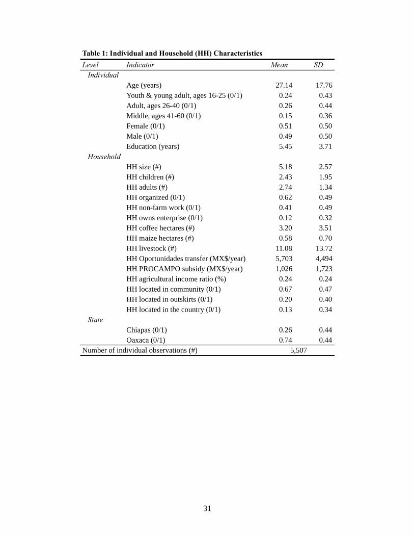
31

Table 1: Individual and Household (HH) Characteristics

Level Indicator Mean SD

Individual

Age (years) 27.14 17.76

Youth & young adult, ages 16-25 (0/1) 0.24 0.43

Adult, ages 26-40 (0/1) 0.26 0.44

Middle, ages 41-60 (0/1) 0.15 0.36

Female (0/1) 0.51 0.50

Male (0/1) 0.49 0.50

Education (years) 5.45 3.71

Household

HH size (#) 5.18 2.57

HH children (#) 2.43 1.95

HH adults (#) 2.74 1.34

HH organized (0/1) 0.62 0.49

HH non-farm work (0/1) 0.41 0.49

HH owns enterprise (0/1) 0.12 0.32

HH coffee hectares (#) 3.20 3.51

HH maize hectares (#) 0.58 0.70

HH livestock (#) 11.08 13.72

HH Oportunidades transfer (MX$/year) 5,703 4,494

HH PROCAMPO subsidy (MX$/year) 1,026 1,723

HH agricultural income ratio (%) 0.24 0.24

HH located in community (0/1) 0.67 0.47

HH located in outskirts (0/1) 0.20 0.40

HH located in the country (0/1) 0.13 0.34

State

Chiapas (0/1) 0.26 0.44

Oaxaca (0/1) 0.74 0.44

Number of individual observations (#) 5,507

32

Table 2: Primary Occupation Outcomes for Working Age Individuals (ages 15-60)

Sample

N % Educ N % Educ N % Educ

4 ordered occupation categories

(1) Homemaker 1,464 44.26 4.77 1,464 82.43 4.76 - - -

(2) Agricultural, housekeeping/clean 1,254 37.91 5.27 161 9.08 5.21 1,095 71.38 5.28

(3) Construction, manufacturing, sales, food, service, etc. 437 13.21 6.67 84 4.73 6.71 353 23.01 6.66

(4) Professional or high-skilled, etc. 153 4.63 9.33 67 3.77 8.27 86 5.61 10.13

Total 3,308 100 5.40 1,776 100 5.01 1,534 100 5.85

Notes: 18 unemployed & 376 student observations

Educ is the average years of education for each occupation category.

All Female Male

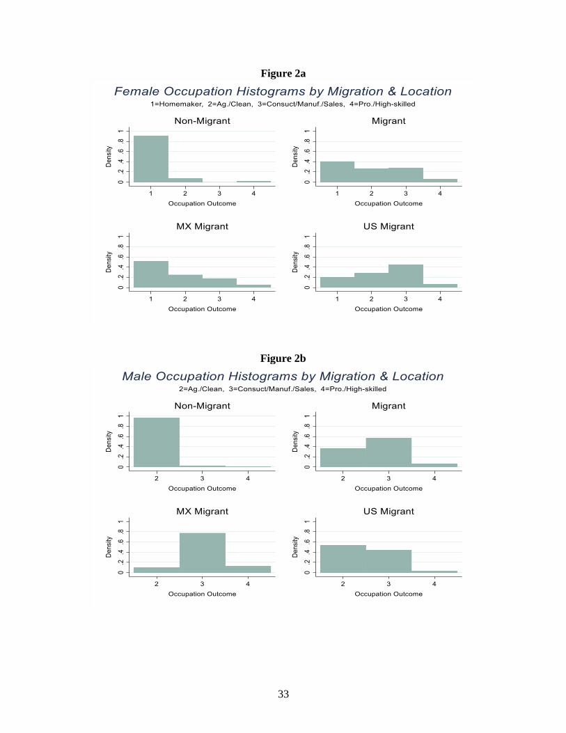
33

Figure 2a

Figure 2b

34

Figure 3a

Figure 3b

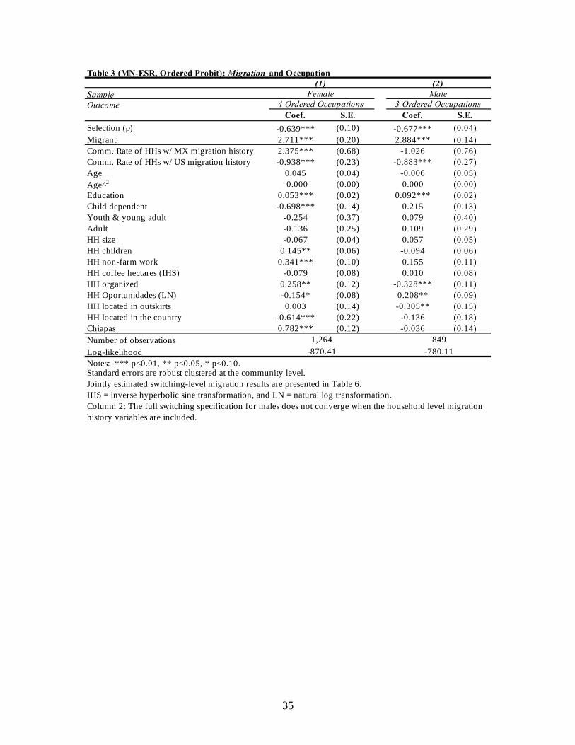
35

Sample

Outcome

Coef. S.E. Coef. S.E.

Selection (ρ) -0.639*** (0.10) -0.677*** (0.04)

Migrant 2.711*** (0.20) 2.884*** (0.14)

Comm. Rate of HHs w/ MX migration history 2.375*** (0.68) -1.026 (0.76)

Comm. Rate of HHs w/ US migration history -0.938*** (0.23) -0.883*** (0.27)

Age 0.045 (0.04) -0.006 (0.05)

Age^2 -0.000 (0.00) 0.000 (0.00)

Education 0.053*** (0.02) 0.092*** (0.02)

Child dependent -0.698*** (0.14) 0.215 (0.13)

Youth & young adult -0.254 (0.37) 0.079 (0.40)

Adult -0.136 (0.25) 0.109 (0.29)

HH size -0.067 (0.04) 0.057 (0.05)

HH children 0.145** (0.06) -0.094 (0.06)

HH non-farm work 0.341*** (0.10) 0.155 (0.11)

HH coffee hectares (IHS) -0.079 (0.08) 0.010 (0.08)

HH organized 0.258** (0.12) -0.328*** (0.11)

HH Oportunidades (LN) -0.154* (0.08) 0.208** (0.09)

HH located in outskirts 0.003 (0.14) -0.305** (0.15)

HH located in the country -0.614*** (0.22) -0.136 (0.18)

Chiapas 0.782*** (0.12) -0.036 (0.14)

Number of observations

Log-likelihood

Notes: *** p<0.01, ** p<0.05, * p<0.10.Standard errors are robust clustered at the community level.

Jointly estimated switching-level migration results are presented in Table 6.

IHS = inverse hyperbolic sine transformation, and LN = natural log transformation.

Column 2: The full switching specification for males does not converge when the household level migration

history variables are included.

Female

4 Ordered Occupations

Male

3 Ordered Occupations

Table 3 (MN-ESR, Ordered Probit): Migration and Occupation

(1) (2)

-780.11

1,264 849

-870.41

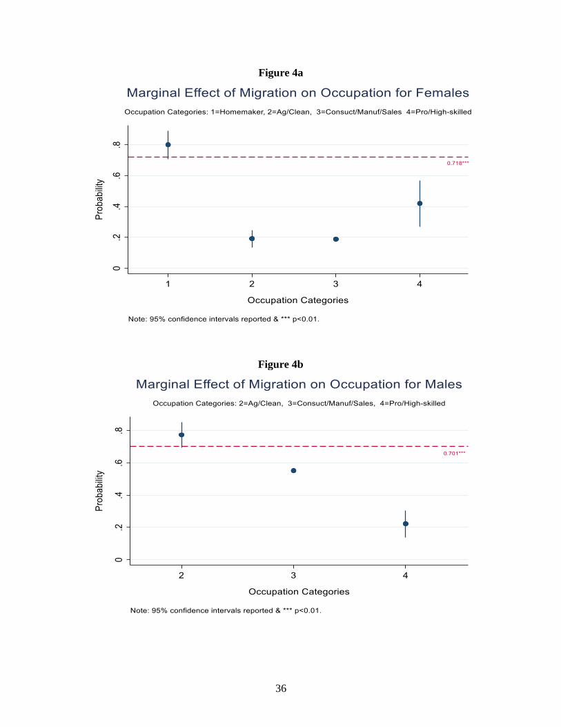
36

Figure 4a

Figure 4b

37

Sample

Outcome

Coef. S.E. Coef. S.E.

Selection (ρ) -0.405** (0.16) -0.061 (0.25)

Return migrant 1.758*** (0.28) 1.533*** (0.39)

Comm. Rate of HHs w/ MX migration history 2.849*** (0.73) - -

Comm. Rate of HHs w/ US migration history -1.466*** (0.26) - -

Age 0.098** (0.04) 0.014 (0.06)

Age^2 -0.001* (0.00) -0.000 (0.00)

Education 0.097*** (0.02) 0.161*** (0.02)

Child dependent -0.695*** (0.13) 0.309* (0.17)

Youth & young adult -0.089 (0.35) 0.290 (0.43)

Adult -0.074 (0.23) 0.127 (0.29)

HH size -0.025 (0.04) -0.063 (0.05)

HH children 0.003 (0.05) -0.042 (0.07)

HH non-farm work 0.272*** (0.10) 0.205* (0.12)

HH coffee hectares (IHS) -0.069 (0.07) -0.046 (0.08)

HH organized 0.128 (0.11) -0.154 (0.12)

HH Oportunidades (LN) -0.121 (0.08) 0.061 (0.10)

HH located in outskirts -0.116 (0.14) 0.134 (0.15)

HH located in the country 0.012 (0.17) -0.521** (0.21)

Chiapas 0.692*** (0.11) -1.715*** (0.23)

Number of observations

Log-likelihood

Notes: *** p<0.01, ** p<0.05, * p<0.10.Standard errors are robust clustered at the community level.

Jointly estimated switching-level return migration results are presented in Appendix Table 1.

IHS = inverse hyperbolic sine transformation, and LN = natural log transformation.

Table 4 (MN-ESR, Ordered Probit): Return Migration and Occupation

(1) (2)

Female

4 Ordered Occupations

Male

3 Ordered Occupations

Column 2: The full switching specification for males does not converge when the household or community

level migration history variables are included.

959

-1,133.07 -914.36

1,377

38

Figure 5a

Figure 5b

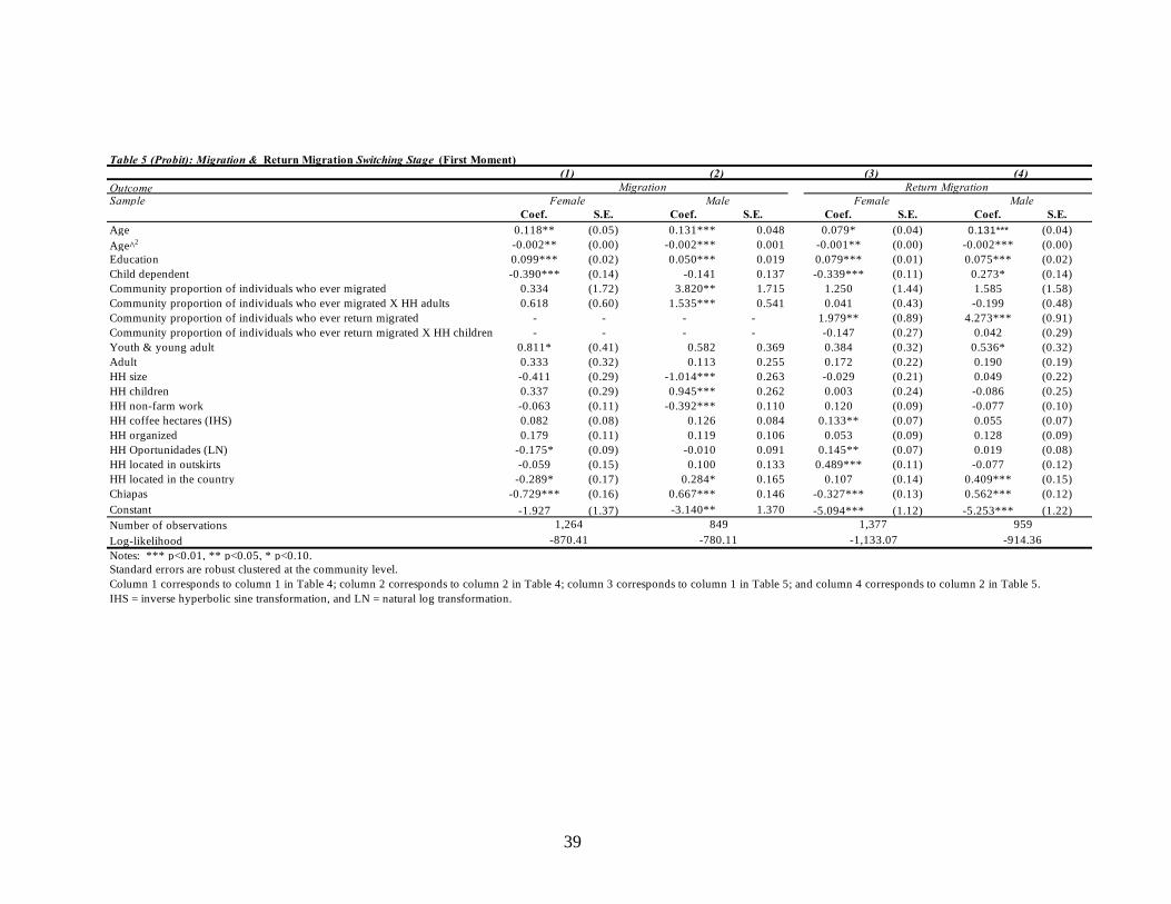
39

OutcomeSample

Coef. S.E. Coef. S.E. Coef. S.E. Coef. S.E.

Age 0.118** (0.05) 0.131*** 0.048 0.079* (0.04) 0.131*** (0.04)

Age^2 -0.002** (0.00) -0.002*** 0.001 -0.001** (0.00) -0.002*** (0.00)

Education 0.099*** (0.02) 0.050*** 0.019 0.079*** (0.01) 0.075*** (0.02)

Child dependent -0.390*** (0.14) -0.141 0.137 -0.339*** (0.11) 0.273* (0.14)

Community proportion of individuals who ever migrated 0.334 (1.72) 3.820** 1.715 1.250 (1.44) 1.585 (1.58)

Community proportion of individuals who ever migrated X HH adults 0.618 (0.60) 1.535*** 0.541 0.041 (0.43) -0.199 (0.48)

Community proportion of individuals who ever return migrated - - - - 1.979** (0.89) 4.273*** (0.91)

Community proportion of individuals who ever return migrated X HH children - - - - -0.147 (0.27) 0.042 (0.29)

Youth & young adult 0.811* (0.41) 0.582 0.369 0.384 (0.32) 0.536* (0.32)

Adult 0.333 (0.32) 0.113 0.255 0.172 (0.22) 0.190 (0.19)

HH size -0.411 (0.29) -1.014*** 0.263 -0.029 (0.21) 0.049 (0.22)

HH children 0.337 (0.29) 0.945*** 0.262 0.003 (0.24) -0.086 (0.25)

HH non-farm work -0.063 (0.11) -0.392*** 0.110 0.120 (0.09) -0.077 (0.10)

HH coffee hectares (IHS) 0.082 (0.08) 0.126 0.084 0.133** (0.07) 0.055 (0.07)

HH organized 0.179 (0.11) 0.119 0.106 0.053 (0.09) 0.128 (0.09)

HH Oportunidades (LN) -0.175* (0.09) -0.010 0.091 0.145** (0.07) 0.019 (0.08)

HH located in outskirts -0.059 (0.15) 0.100 0.133 0.489*** (0.11) -0.077 (0.12)

HH located in the country -0.289* (0.17) 0.284* 0.165 0.107 (0.14) 0.409*** (0.15)

Chiapas -0.729*** (0.16) 0.667*** 0.146 -0.327*** (0.13) 0.562*** (0.12)

Constant -1.927 (1.37) -3.140** 1.370 -5.094*** (1.12) -5.253*** (1.22)

Number of observations

Log-likelihood

Notes: *** p<0.01, ** p<0.05, * p<0.10.

Standard errors are robust clustered at the community level.

Column 1 corresponds to column 1 in Table 4; column 2 corresponds to column 2 in Table 4; column 3 corresponds to column 1 in Table 5; and column 4 corresponds to column 2 in Table 5.

IHS = inverse hyperbolic sine transformation, and LN = natural log transformation.

Female Male Female Male

1,264 849

Table 5 (Probit): Migration & Return Migration Switching Stage (First Moment)

(1) (2) (3) (4)

1,377 959

Migration Return Migration

-870.41 -780.11 -1,133.07 -914.36

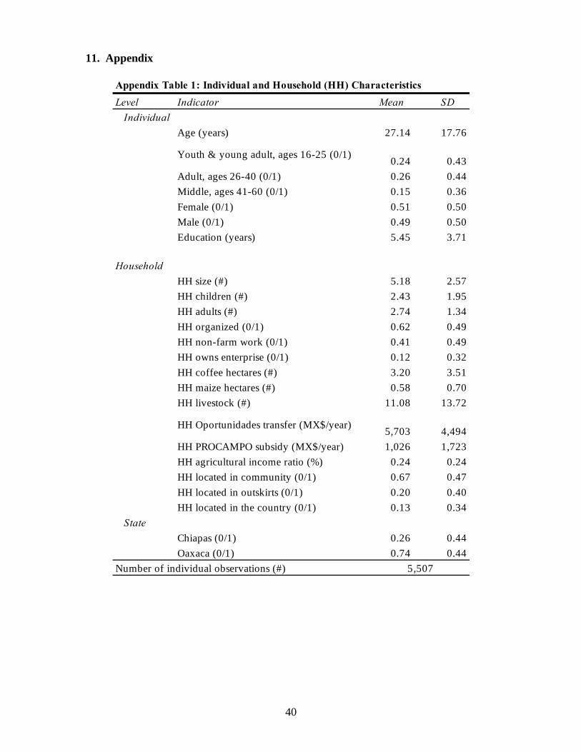
40

11. Appendix

Appendix Table 1: Individual and Household (HH) Characteristics

Level Indicator Mean SD

Individual

Age (years) 27.14 17.76

Youth & young adult, ages 16-25 (0/1)0.24 0.43

Adult, ages 26-40 (0/1) 0.26 0.44

Middle, ages 41-60 (0/1) 0.15 0.36

Female (0/1) 0.51 0.50

Male (0/1) 0.49 0.50

Education (years) 5.45 3.71

Household

HH size (#) 5.18 2.57

HH children (#) 2.43 1.95

HH adults (#) 2.74 1.34

HH organized (0/1) 0.62 0.49

HH non-farm work (0/1) 0.41 0.49

HH owns enterprise (0/1) 0.12 0.32

HH coffee hectares (#) 3.20 3.51

HH maize hectares (#) 0.58 0.70

HH livestock (#) 11.08 13.72

HH Oportunidades transfer (MX$/year)5,703 4,494

HH PROCAMPO subsidy (MX$/year) 1,026 1,723

HH agricultural income ratio (%) 0.24 0.24

HH located in community (0/1) 0.67 0.47

HH located in outskirts (0/1) 0.20 0.40

HH located in the country (0/1) 0.13 0.34

State

Chiapas (0/1) 0.26 0.44

Oaxaca (0/1) 0.74 0.44

Number of individual observations (#) 5,507

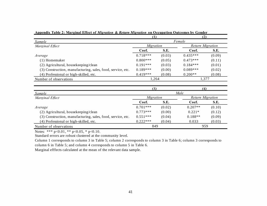
41

Sample

Marginal Effect

Coef. S.E. Coef. S.E.

Average 0.718*** (0.03) 0.435*** (0.09)

(1) Homemaker 0.800*** (0.05) 0.473*** (0.11)

(2) Agricultural, housekeeping/clean 0.191*** (0.03) 0.184*** (0.01)

(3) Construction, manufacturing, sales, food, service, etc. 0.189*** (0.00) 0.089*** (0.02)

(4) Professional or high-skilled, etc. 0.419*** (0.08) 0.200** (0.08)

Number of observations

Sample

Marginal Effect

Coef. S.E. Coef. S.E.

Average 0.701*** (0.02) 0.207** (0.10)

(2) Agricultural, housekeeping/clean 0.773*** (0.00) 0.221* (0.12)

(3) Construction, manufacturing, sales, food, service, etc. 0.551*** (0.04) 0.188** (0.09)

(4) Professional or high-skilled, etc. 0.222*** (0.04) 0.033 (0.03)

Number of observations

Notes: *** p<0.01, ** p<0.05, * p<0.10.Standard errors are robust clustered at the community level.

Marginal efffects calculated at the mean of the relevant data sample.

Column 1 corresponds to column 3 in Table 5; column 2 corresponds to column 3 in Table 6; column 3 corresponds to

column 6 in Table 5; and column 4 corresponds to column 5 in Table 6.

Migration Return Migration

Female

1,264 1,377

Male

Migration Return Migration

(3) (4)

Appendix Table 2: Marginal Effect of Migration & Return Migration on Occupation Outcomes by Gender

(1) (2)

849 959

42

AnalysisSample

Outcome

Coef. S.E. Coef. S.E. Coef. S.E. Coef. S.E.

Migrant 1.675*** (0.19) 2.029*** (0.29) - - - -

Return migrant - - - - 1.070*** (0.20) 1.358*** (0.24)

Age 0.074*** (0.02) 0.019 (0.05) 0.108*** (0.03) 0.031 (0.05)

Age^2 -0.001* (0.00) -0.000 (0.00) -0.001*** (0.00) -0.000 (0.00)

Education 0.077*** (0.02) 0.127*** (0.02) 0.116*** (0.03) 0.159*** (0.03)

Child dependent 2.841*** (0.94) 0.162 (1.05) -0.788*** (0.17) 0.306 (0.25)

Comm. Rate of HHs w/ MX migration history -0.994** (0.45) -0.744** (0.32) 3.320*** (0.62) -1.081 (1.20)

Comm. Rate of HHs w/ US migration history -0.838*** (0.14) 0.151 (0.13) -1.456*** (0.38) -0.284 (0.52)

Youth & young adult 0.025 (0.27) 0.344 (0.22) 0.004 (0.20) 0.360 (0.36)

Adult -0.045 (0.22) 0.209 (0.29) -0.025 (0.17) 0.164 (0.36)

HH size -0.102 (0.07) -0.054 (0.03) -0.033 (0.05) -0.054 (0.06)

HH children 0.161** (0.08) -0.010 (0.05) -0.007 (0.04) -0.029 (0.08)

HH non-farm work 0.438*** (0.07) 0.111* (0.07) 0.309*** (0.08) 0.204 (0.21)

HH coffee hectares (IHS) -0.089 (0.11) 0.028 (0.11) -0.041 (0.07) -0.048 (0.09)

HH organized 0.335** (0.15) -0.334*** (0.09) 0.148 (0.10) -0.172 (0.13)

HH Oportunidades (LN) -0.186 (0.14) 0.238*** (0.09) -0.098 (0.13) 0.066 (0.08)

HH located in outskirts 0.016 (0.17) -0.344*** (0.10) -0.004 (0.17) 0.166 (0.15)

HH located in the country -0.720*** (0.21) -0.173 (0.20) 0.009 (0.19) -0.439** (0.19)

Chiapas 0.699*** (0.17) -0.023 (0.13) 0.663*** (0.16) -1.733*** (0.23)

Number of observations

Log-likelihood

Notes: *** p<0.01, ** p<0.05, * p<0.10.Standard errors are robust clustered at the community level.Column 1 corresponds to column 1 in Table 3; column 2 corresponds to column 2 in Table 2; column 3 corresponds to column 1 in Table 4; and column 4 corresponds to column 2 in Table 4.

IHS = inverse hyperbolic sine transformation, and LN = natural log transformation.

1,377 959

-350.55

1,264

-510.81

849

-374.44 -556.65

Appendix Table 3 (Ordered Probit): Naïve Regressions for Migrants & Return Migrants & Occupation

3 Ordered Occupations

(4)

3 Ordered OccupationsMale

Return Migration

(1) (2) (3)

Migration

4 Ordered OccupationsFemale Male

4 Ordered OccupationsFemale

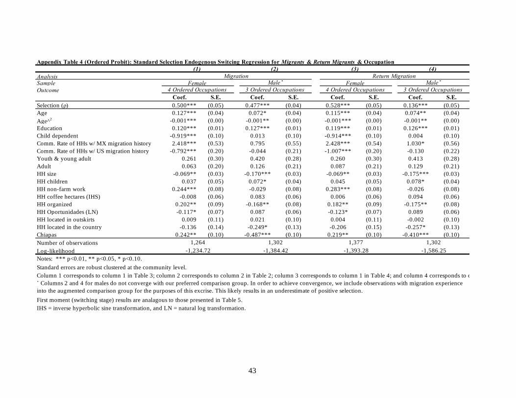
43

AnalysisSample

Outcome

Coef. S.E. Coef. S.E. Coef. S.E. Coef. S.E.

Selection (ρ) 0.500*** (0.05) 0.477*** (0.04) 0.528*** (0.05) 0.136*** (0.05)

Age 0.127*** (0.04) 0.072* (0.04) 0.115*** (0.04) 0.074** (0.04)

Age^2 -0.001*** (0.00) -0.001** (0.00) -0.001*** (0.00) -0.001** (0.00)

Education 0.120*** (0.01) 0.127*** (0.01) 0.119*** (0.01) 0.126*** (0.01)

Child dependent -0.919*** (0.10) 0.013 (0.10) -0.914*** (0.10) 0.004 (0.10)

Comm. Rate of HHs w/ MX migration history 2.418*** (0.53) 0.795 (0.55) 2.428*** (0.54) 1.030* (0.56)

Comm. Rate of HHs w/ US migration history -0.792*** (0.20) -0.044 (0.21) -1.007*** (0.20) -0.130 (0.22)

Youth & young adult 0.261 (0.30) 0.420 (0.28) 0.260 (0.30) 0.413 (0.28)

Adult 0.063 (0.20) 0.126 (0.21) 0.087 (0.21) 0.129 (0.21)

HH size -0.069** (0.03) -0.170*** (0.03) -0.069** (0.03) -0.175*** (0.03)

HH children 0.037 (0.05) 0.072* (0.04) 0.045 (0.05) 0.078* (0.04)

HH non-farm work 0.244*** (0.08) -0.029 (0.08) 0.283*** (0.08) -0.026 (0.08)

HH coffee hectares (IHS) -0.008 (0.06) 0.083 (0.06) 0.006 (0.06) 0.094 (0.06)

HH organized 0.202** (0.09) -0.168** (0.08) 0.182** (0.09) -0.175** (0.08)

HH Oportunidades (LN) -0.117* (0.07) 0.087 (0.06) -0.123* (0.07) 0.089 (0.06)

HH located in outskirts 0.009 (0.11) 0.021 (0.10) 0.004 (0.11) -0.002 (0.10)

HH located in the country -0.136 (0.14) -0.249* (0.13) -0.206 (0.15) -0.257* (0.13)

Chiapas 0.242** (0.10) -0.487*** (0.10) 0.219** (0.10) -0.410*** (0.10)

Number of observations

Log-likelihood

Notes: *** p<0.01, ** p<0.05, * p<0.10.

Standard errors are robust clustered at the community level.

Column 1 corresponds to column 1 in Table 3; column 2 corresponds to column 2 in Table 2; column 3 corresponds to column 1 in Table 4; and column 4 corresponds to column 2 in Table 4.

First moment (switching stage) results are analagous to those presented in Table 5.

IHS = inverse hyperbolic sine transformation, and LN = natural log transformation.

Migration Return Migration

Appendix Table 4 (Ordered Probit): Standard Selection Endogenous Switcing Regression for Migrants & Return Migrants & Occupation

(1) (2) (3) (4)

Female Male ˚ Female Male ˚4 Ordered Occupations 3 Ordered Occupations 4 Ordered Occupations 3 Ordered Occupations

˚ Columns 2 and 4 for males do not converge with our preferred comparison group. In order to achieve convergence, we include observations with migration experience

into the augmented comparison group for the purposes of this excrise. This likely results in an underestimate of positive selection.

1,264 1,302 1,377 1,302

-1,234.72 -1,384.42 -1,393.28 -1,586.25

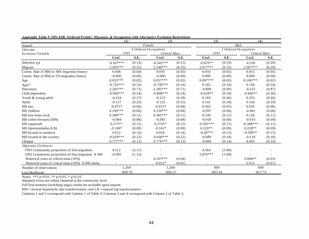
44

Sample

Outcome

Exclusion Variable

Coef. S.E. Coef. S.E. Coef. S.E. Coef. S.E.

Selection (ρ) -0.567*** (0.14) -0.542*** (0.15) -0.470** (0.19) -0.330 (0.20)

Migrant 2.593*** (0.25) 2.549*** (0.25) 2.677*** (0.25) 2.507*** (0.29)

Comm. Rate of HHs w/ MX migration history 0.048 (0.04) 0.050 (0.05) 0.010 (0.05) 0.015 (0.05)

Comm. Rate of HHs w/ US migration history -0.000 (0.00) -0.000 (0.00) 0.000 (0.00) 0.000 (0.00)

Age 0.055*** (0.02) 0.057*** (0.02) 0.097*** (0.02) 0.106*** (0.02)

Age^2 -0.722*** (0.14) -0.730*** (0.14) 0.162 (0.14) 0.156 (0.14)

Education 2.285*** (0.71) 2.385*** (0.71) -0.809 (0.90) -0.253 (0.87)

Child dependent -0.900*** (0.24) -0.898*** (0.24) -0.658** (0.29) -0.666** (0.30)

Youth & young adult -0.224 (0.37) -0.213 (0.38) 0.183 (0.40) 0.233 (0.40)

Adult -0.127 (0.25) -0.125 (0.25) 0.141 (0.28) 0.164 (0.29)

HH size -0.071* (0.04) -0.072* (0.04) 0.043 (0.05) 0.020 (0.06)

HH children 0.149*** (0.06) 0.150*** (0.06) -0.097 (0.06) -0.081 (0.06)

HH non-farm work 0.360*** (0.11) 0.365*** (0.11) 0.140 (0.11) 0.126 (0.11)

HH coffee hectares (IHS) -0.084 (0.08) -0.085 (0.08) -0.018 (0.08) -0.014 (0.09)

HH organized 0.273** (0.12) 0.274** (0.12) -0.302*** (0.11) -0.308*** (0.11)

HH Oportunidades (LN) -0.160* (0.09) -0.161* (0.09) 0.220** (0.09) 0.228** (0.09)

HH located in outskirts 0.012 (0.14) 0.016 (0.14) -0.287** (0.15) -0.299** (0.15)

HH located in the country -0.629*** (0.22) -0.640*** (0.22) -0.089 (0.18) -0.118 (0.18)

Chiapas 0.777*** (0.12) 0.776*** (0.12) -0.009 (0.14) 0.003 (0.14)

Migration Exclusions

1995 Community proportion of first migration 4.512 (3.11) - - 4.564 (3.06) - -

1995 Community proportion of first migration X HH -0.085 (1.12) - - 2.876*** (1.08) - -

Historical years of critical mass (10%) - - 0.107*** (0.04) - - 0.068** (0.03)

Historical years of critical mass (10%) X HH adults - - -0.022* (0.01) - - 0.012 (0.01)

Number of observations

Log-likelihood

Notes: *** p<0.01, ** p<0.05, * p<0.10.Standard errors are robust clustered at the community level.

Full first moment (switching stage) results are available upon request.

IHS = inverse hyperbolic sine transformation, and LN = natural log transformation.

Columns 1 and 2 correspond with Column 1 of Table 3; Columns 3 and 4 correspond with Column 2 of Table 3.

Apptendix Table 5 (MN-ESR, Ordered Probit): Migration & Occupation with Alternative Exclusion Restrictions

(1) (4)

Female

4 Ordered Occupations

-868.76 -817.73

(2)

1,264

-866.37

1995 Critical Mass

(3)

8491,264

-803.44

Male

3 Ordered Occupations

1995 Critical Mass

849

45

Sample

Outcome

Exclusion Variable

Coef. S.E. Coef. S.E. Coef. S.E. Coef. S.E.

Selection (ρ) -0.341* (0.18) -0.354** (0.18) -0.632*** (0.15) -0.646*** (0.14)

Return Migrant 1.653*** (0.33) 1.672*** (0.31) 2.356*** (0.21) 2.361*** (0.20)

Comm. Rate of HHs w/ MX migration history 0.100** (0.04) 0.100** (0.04) -0.021 (0.05) -0.023 (0.05)

Comm. Rate of HHs w/ US migration history -0.001* (0.00) -0.001* (0.00) 0.000 (0.00) 0.000 (0.00)

Age 0.100*** (0.02) 0.100*** (0.02) 0.104*** (0.02) 0.103*** (0.02)

Age^2 -0.714*** (0.14) -0.711*** (0.13) 0.087 (0.16) 0.088 (0.16)

Education 2.991*** (0.73) 3.042*** (0.72) -1.379* (0.76) -1.156 (0.75)

Child dependent -1.435*** (0.26) -1.413*** (0.26) -0.312 (0.32) -0.278 (0.32)

Youth & young adult -0.069 (0.35) -0.071 (0.35) 0.083 (0.38) 0.079 (0.38)

Adult -0.064 (0.23) -0.066 (0.23) 0.070 (0.24) 0.068 (0.24)

HH size -0.028 (0.04) -0.028 (0.04) -0.003 (0.04) -0.005 (0.04)

HH children 0.002 (0.05) 0.002 (0.05) -0.098* (0.06) -0.097* (0.06)

HH non-farm work 0.277*** (0.10) 0.275*** (0.10) 0.170 (0.11) 0.161 (0.11)

HH coffee hectares (IHS) -0.069 (0.07) -0.072 (0.07) -0.075 (0.07) -0.079 (0.07)

HH organized 0.134 (0.11) 0.133 (0.11) -0.137 (0.11) -0.129 (0.11)

HH Oportunidades (LN) -0.120 (0.08) -0.121 (0.08) 0.072 (0.09) 0.072 (0.08)

HH located in outskirts -0.099 (0.14) -0.104 (0.14) 0.102 (0.14) 0.096 (0.14)

HH located in the country 0.003 (0.17) 0.001 (0.17) -0.458** (0.18) -0.480*** (0.18)

Chiapas 0.697*** (0.12) 0.698*** (0.12) -1.403*** (0.18) -1.396*** (0.18)

Migration Exclusions

1995 Community proportion of first return migration 5.347** (2.64) - - 5.085** (2.57) - -

1995 Community proportion of first return migration X HH -0.398 (0.87) - - -0.011 (0.86) - -

Historical years of critical mass (10%) - - 0.074*** (0.03) - - 0.040 (0.03)

Historical years of critical mass (10%) X HH children - - -0.012 (0.01) - - -0.001 (0.01)

Number of observations

Log-likelihood

Notes: *** p<0.01, ** p<0.05, * p<0.10.Standard errors are robust clustered at the community level.

Full first moment (switching stage) results are available upon request.

IHS = inverse hyperbolic sine transformation, and LN = natural log transformation.

Columns 1 and 2 correspond with Column 1 of Table 4; Columns 3 and 4 correspond with Column 2 of Table 4.

Female Male

Apptendix Table 6 (MN-ESR, Ordered Probit): Return Migration & Occupation with Alternative Exclusion Restrictions

(1) (2) (3) (4)

4 Ordered Occupations 3 Ordered Occupations

1995 Critical Mass 1995 Critical Mass

1,377 1,377 959 959

-1,136.51 -1,137.01 -959.37 -963.30