Embed Size (px)
Citation preview

YEAR/SEM-Y2/S3 DATA STRUCTURES- UNIT II
1
DEPT OF CSE,RGCET
UNIT 2
Stacks: Definition – operations - applications of stack. Queues: Definition -
operations - Priority queues - De queues – Applications of queue. Linked List:
Singly Linked List, Doubly Linked List, Circular Linked List, linked stacks, Linked
queues, Applications of Linked List – Dynamic storage management – Generalized
list.
Abstract Data Types (ADTs)
An Abstract Data Type (ADT) is a set of operations. Abstract data types are mathematical
abstractions; nowhere in an ADT's definition is there any mention of how the set of
operations is implemented. This can be viewed as an extension of modular design.
Objects such as lists, sets, and graphs, along with their operations, can be viewed as abstract
data types, just as integers, reals, and booleans are data types. Integers, reals, and booleans
have operations associated with them, and so do abstract data types. For the set ADT, there
are various operations as union, intersection, size, and complement. Alternately, the two
operations union and find, which would define a different ADT on the set.
The basic idea is that the implementation of these operations is written once in the program,
and any other part of the program that needs to perform an operation on the ADT can do so
by calling the appropriate function. If for some reason implementation details need to
change, it should be easy to do so by merely changing the routines that perform the ADT
operations. This change, in a perfect world, would be completely transparent to the rest of
the program.
THE STACK ADT
What is stack? How would you perform the operations on stack? How the stack is useful to
evaluate the expression? (11 Marks Nov 2010)
Explain Stack and its Operation with neat diagram. (6 Marks Apr 2013,Nov 2014)
Describe the procedures ADD and DELETE operations on stack.(11 Marks Nov 2013)

YEAR/SEM-Y2/S3 DATA STRUCTURES- UNIT II
2
DEPT OF CSE,RGCET
A stack is a list with the restriction that inserts and deletes can be performed in only one
position, namely the end of the list called the top.
The fundamental operations on a stack are push, which is equivalent to an insert, and pop,
which deletes the most recently inserted element.
The most recently inserted element can be examined prior to performing a pop by use of the
top routine.
A pop or top on an empty stack is generally considered an error in the stack ADT. On the
other hand, running out of space when performing a push is an implementation error but not
an ADT error.
Stacks are sometimes known as LIFO (last in, first out) lists. The usual operations to make
empty stacks and test for emptiness are part of the repertoire, but essentially all that you can
do to a stack is push and pop.
Stack model: input to a stack is by push, output is by pop
Stack model: only the top element is accessible
YEAR/SEM-Y2/S3 DATA STRUCTURES- UNIT II
3
DEPT OF CSE,RGCET
BASIC OPERATION ON A STACK (***)
1. Create a stack
2. Push an element onto a stack
3. Pop an element from a stack
4. Print the entire stack
5. Read the top of the stack
6. Check whether the stack is empty or full
PUSH OPERATION:
Push operation inserts an element onto the stack.
An attempt to push an element onto the stack , when the stack is full, causes an overflow.
Push operation involves:
1. Check whether the stack is full before attempting to push an element to the stack.
2. Increment the top pointer.
3. Push the element onto the top of the stack.
ALGORITHM:
STACK - Array to hold elements
N – Total number of elements
TOP – Denotes the top element in the stack
Item – The element to be inserted at the top of a stack
1. if(TOP>=N) [Check for stack overflow]
Then CALL STACK_FULL
Exit
2. TOP<-TOP+1 [Increment TOP]
3. STACK [TOP]<-Item [Insert element]
End PUSH
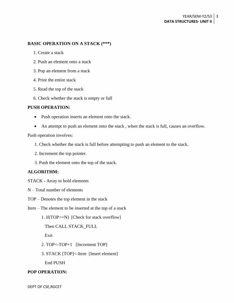
POP OPERATION:
YEAR/SEM-Y2/S3 DATA STRUCTURES- UNIT II
4
DEPT OF CSE,RGCET
POP operation removes an element from the stack.
An attempt to pop an element from the stack, when the array is empty, causes an underflow.
Pop operation involves:
1. Check whether the stack is empty before attempting to pop an element from the stack.
2. Decrement the top pointer.
3. Pop the element from the top of the stack.
ALGORITHM:
STACK – Array to hold elements
TOP – Denotes the top element in the stack
Item – The element to be deleted from the top of the stack
1. If (TOP<=0) [Check for underflow on stack]
Then Call STACK_EMPTY - Exit
2. Item<-STACK [TOP] [Return top element of the stack]
3. TOP<-TOP-1 [Decrement top pointer]
If stack is implemented using array it cannot grow dynamically where as Linked stack can grow
dynamically.
IMPLEMENTATION OF STACKS
There are two implementations.
Pointers implementation
Array implementation.
Array Implementation of Stacks
Structure Definition
struct stack_record
{
unsigned int stack_size; //size of the stack
int top_of_stack; // top of the stack
element_type *stack_array; // pointer to an array

YEAR/SEM-Y2/S3 DATA STRUCTURES- UNIT II
5
DEPT OF CSE,RGCET
};
typedef struct stack_record *STACK;
Function to dispose a stack
This function not only frees the memory allocated for the stack (array) but also the structure
containing the details of the stack.
void dispose_stack( STACK S )
{
if( S != NULL )
{
free( S->stack_array );
free( S );
}
}
Function to empty a stack
If the stack is not empty, the stack is popped until it becomes empty. In other words, the
stack exists but the stack is empty.
void make_Empty( STACK S )
{
S->top_of_stack = EMPTY_TOS;
}
Function to check whether the stack is empty
This function checks whether the stack is empty or not. The function is_empty ()
returns S->top_of_stack == EMPTY_TOS in case the stack is empty.
int is_empty( STACK S )
{
return( S->top_of_stack = = EMPTY_TOS );
}

YEAR/SEM-Y2/S3 DATA STRUCTURES- UNIT II
6
DEPT OF CSE,RGCET
Function to check whether the stack is full
This function checks whether the stack is full or not. The function is_full () returns
S->top_of_stack = max_elements in case the stack is full.
int is_empty( STACK S )
{
return( S->top_of_stack = = max_elements );
}
Function to push an element into the stack
To push an element into the stack, move to the next location in the array, insert the value
and make S->top_of_stack to point to that element.
void push( element_type x, STACK S )
{
if( is_full( S ) )
error("Full stack");
else
S->stack_array[ ++S->top_of_stack ] = x;
}
Function to return the top element from the stack
Check whether the stack is empty. If the stack is not empty, the element pointed to by S->
top_of_stack is returned from the stack.
element_type top( STACK S )
{
if( is_empty( S ) )
error("Empty stack");
else
return S->stack_array[ S->top_of_stack ];
}

YEAR/SEM-Y2/S3 DATA STRUCTURES- UNIT II
7
DEPT OF CSE,RGCET
Function to pop an element from the stack
Check whether the stack is empty. If the stack is not empty the element
pointed to by S->top_of_stack should be removed from the stack. This is done by decrementing the
S->top_of_stack pointer.
void pop( STACK S )
{
if( is_empty( S ) )
error("Empty stack");
else
S->stack_array [ S->top_of_stack - -];
}
Function to return the top element and pop an element from the stack
Check whether the stack is empty. If the stack is not empty, the element pointed to by
S->top_of_stack is returned and removed from the stack. This is done by decrementing the S->
top_of_stack pointer.
element_type pop( STACK S )
{
if( is_empty( S ) )
error("Empty stack");
else
return S->stack_array[ S->top_of_stack - - ];
}
One problem that affects the efficiency of implementing stacks is error testing.
As described above, a pop on an empty stack or a push on a full stack will overflow the
array bounds and cause a crash. This is obviously undesirable, but if checks for these
conditions were put in the array implementation, they would likely take as much time as the
actual stack manipulation.

YEAR/SEM-Y2/S3 DATA STRUCTURES- UNIT II
8
DEPT OF CSE,RGCET
Declare the stack to be large enough not to overflow and ensure that routines that use pop
never attempt to pop an empty stack, this can lead to code that barely works at best,
especially when programs get large.
Because stack operations take such fast constant time, it is rare that a significant part of the
running time of a program is spent in these routines. This means that it is generally not
justifiable to omit error checks.
APPLICATIONS OF STACK
Convert the following infix expression to postfix expression.((A+B)^C-(D*E)/F)
11 Marks April 2015 //Refer notebook for Answer//
Explain the process of conversion from infix expression to postfix expression
using stack. (11 Marks April 2014)
Convert the following in reverse polish notation. Show the stack operations. (A-B)*(C(D+E-
F*(G)/H)) 11 Marks April 2015 //Refer notebook for answer//
Write about Recursive Function. (11 Marks April 2013)
The various applications of a stack are
Infix into postfix Expression.
Evaluation of postfix Expression.
Implementation of Recursion
Factorial
Quick Sort
Tower of hanoi
1. Infix to Postfix Conversion (***)
Not only can a stack be used to evaluate a postfix expression, but a stack can be used to
convert an expression in standard form (otherwise known as infix) into postfix. A small version of

YEAR/SEM-Y2/S3 DATA STRUCTURES- UNIT II
9
DEPT OF CSE,RGCET
the general problem by involves only the operators +, *, and (,), and insisting on the usual
precedence rules. Assume that the expression is legal. Suppose the infix expression is to be
converted into postfix.
a + b * c + ( d * e + f ) * g
A correct answer is a b c * + d e * f + g * +.
When an operand is read, it is immediately placed onto the output.
Operators are not immediately output, so they must be saved somewhere. The correct thing
to do is to place operators that have been seen, but not placed on the output, onto the stack.
Stack left parentheses when they are encountered.
Start with an initially empty stack.
If a right parenthesis is encountered, then pop the stack, writing symbols until a
(corresponding) left parenthesis is encountered, which is popped but not output.
If any other symbol ('+','*', '(' ) is seen, then pop entries from the stack until an entry of
lower priority is found.
One exception is that never remove a '(' from the stack except when processing a ')'. For the
purposes of this operation, '+' has lowest priority and '(' highest.
When the popping is done, push the operand onto the stack.
Finally, if the end of input is read, pop the stack until it is empty, writing symbols onto the
output.
To see how this algorithm performs, convert the infix expression above into its postfix form.
First, the symbol a is read, so it is passed through to the output. Then '+' is read and pushed
onto the stack. Next b is read and passed through to the output. The state of affairs at this
juncture is as follows:
Next a '*' is read. The top entry on the operator stack has lower precedence than '*', so nothing is
output and '*' is put on the stack. Next, c is read and output. Thus far,
YEAR/SEM-Y2/S3 DATA STRUCTURES- UNIT II
10
DEPT OF CSE,RGCET
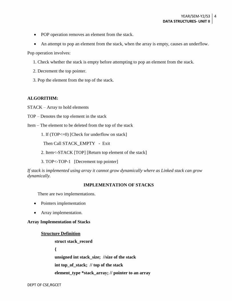
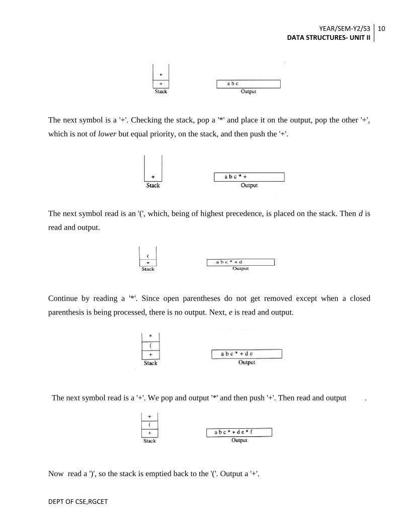
The next symbol is a '+'. Checking the stack, pop a '*' and place it on the output, pop the other '+',
which is not of lower but equal priority, on the stack, and then push the '+'.
The next symbol read is an '(', which, being of highest precedence, is placed on the stack. Then d is
read and output.
Continue by reading a '*'. Since open parentheses do not get removed except when a closed
parenthesis is being processed, there is no output. Next, e is read and output.
The next symbol read is a '+'. We pop and output '*' and then push '+'. Then read and output .
Now read a ')', so the stack is emptied back to the '('. Output a '+'.
YEAR/SEM-Y2/S3 DATA STRUCTURES- UNIT II
11
DEPT OF CSE,RGCET
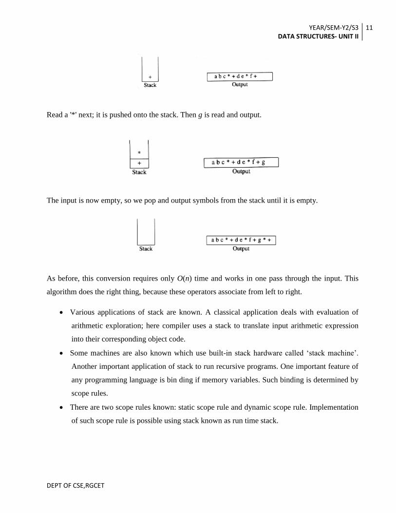
Read a '*' next; it is pushed onto the stack. Then g is read and output.
The input is now empty, so we pop and output symbols from the stack until it is empty.
As before, this conversion requires only O(n) time and works in one pass through the input. This
algorithm does the right thing, because these operators associate from left to right.
Various applications of stack are known. A classical application deals with evaluation of
arithmetic exploration; here compiler uses a stack to translate input arithmetic expression
into their corresponding object code.
Some machines are also known which use built-in stack hardware called ‘stack machine’.
Another important application of stack to run recursive programs. One important feature of
any programming language is bin ding if memory variables. Such binding is determined by
scope rules.
There are two scope rules known: static scope rule and dynamic scope rule. Implementation
of such scope rule is possible using stack known as run time stack.

YEAR/SEM-Y2/S3 DATA STRUCTURES- UNIT II
12
DEPT OF CSE,RGCET
2. Evaluation of Postfix Expressions (***)
When a number is seen, it is pushed onto the stack; when an operator is seen, the operator is
applied to the two numbers (symbols) that are popped from the stack and the result is
pushed onto the stack. For instance, the postfix expression
6 5 2 3 + 8 * + 3 + *
is evaluated as follows: The first four symbols are placed on the stack. The resulting stack is
Next a '+' is read, so 3 and 2 are popped from the stack and their sum, 5, is pushed.
Next 8 is pushed.
Now a '*' is seen, so 8 and 5 are popped as 8 * 5 = 40 is pushed.

YEAR/SEM-Y2/S3 DATA STRUCTURES- UNIT II
13
DEPT OF CSE,RGCET
Next a '+' is seen, so 40 and 5 are popped and 40 + 5 = 45 is pushed.
Now, 3 is pushed.
Next '+' pops 3 and 45 and pushes 45 + 3 = 48.
Finally, a '*' is seen and 48 and 6 are popped, the result 6 * 48 = 288 is pushed.
The time to evaluate a postfix expression is O(n), because processing each element in the input
consists of stack operations and thus takes constant time. The algorithm to do so is very simple.
Notice that when an expression is given in postfix notation, there is no need to know any
precedence rules; this is an obvious advantage.

YEAR/SEM-Y2/S3 DATA STRUCTURES- UNIT II
14
DEPT OF CSE,RGCET
3 ) Implementation of Recursion(**)
Recursion is an important tool to describe a procedure having several repetitions of the
same.
A procedure is termed as recursive if the procedure is defined by itself. As a simple ex, let
us consider the case of calculation of factorial value for an integer n.
n!=n x (n-l) x (n-2) x…. x 3 x 2 x 1
or
n!=n x (n-l)!
factorial (n):
l. fact=1
2.FoR(I=1 to N)do
1.FACT= i *fact
3. EndFor
4. return (fact)
5. Stop
(d ) Factorial calculation
The recursive algorithm to compute n! may be directly translated into a c function as
follows:
int fact (int n)
{
int x,y;
if(n==0)
return (1);
x=n-1;
y=fact (x);
return(n*y);
}/*end fact */

YEAR/SEM-Y2/S3 DATA STRUCTURES- UNIT II
15
DEPT OF CSE,RGCET
In the statement y=fact (x); the function fact calls itself. This is the essential ingredient of a
recursive routine. However this must not lead to an endless series of calls.
For example , suppose that the calling program contains the statement
printf(“%d”,fact (4));
When the calling routine calls “fact” , the parameter n is set equal to 4.
Since n is not 0, x is set value to 3. At that point, fact is called a second time with an
argument of 3.Therefore, the function fact is reentered and the local variables(x and y) and
parameter (n) of the block is reallocated. Since execution is not yet left the first call of fact,
the first allocation of these variables remains.
Thus there are two generations of each of variables in existence simultaneously. From any
point within the second execution of fact, only the most recent copy of these variables are
referenced.
In general, each time the function fact is entered recursively, a new set may be referenced
within that call of fact. When a return from fact to a point in a previous call takes place, the
most recent allocation of these variables is freed, and the previous copy is reactivated. This
previous copy is the one that was allocated upon the original entry to the previous call and is
local to that call.
This description suggests the use of a stack to keep the successive generations of local
variables and parameters.
This stack is maintained by the C system and is invisible to the user. Each time that a
recursive function is entered, a new allocation of its variables is pushed on top of the stack.
Any reference to a local variable or parameters is through the current top of the stack. When
the function returns, the stack is popped, the top allocation is freed and the previous
allocation becomes the current stack top to be used for referencing local variables.
The above figure contains a series of snapshots of the stacks for the variables n,x,and y as
execution of fact function proceeds .Initially ,the stack is empty ,as illustrated in figure.
After the first call on fact by calling procedure, the situation is as shown in the figure, with n
equal to 4.The variables x and y are allocated but not initialized .Since n does not equal 0, x
is set to 3 and fact (3) is called .The new value of n does not equal 0; therefore x is set to 2
and fact(2) is called.

YEAR/SEM-Y2/S3 DATA STRUCTURES- UNIT II
16
DEPT OF CSE,RGCET
This continues until n equals 0. At that point the value 1 is returned from the call to fact(0).
Execution resumes from the point at which fact(0) was called, which is the assignment of the
returned value to the copy of declared in fact(1).This is illustrated by the status of the stack
shown in figure , where the variables allocated for fact(0) have been freed and y is set to 1.
The statement return (n*y) is then executed ,multiplying the top values of n and y to obtain 1
and returning this value to fact(2).This process is repeated twice more , until finally the
value of y in fact(4) equals 6. The statement return(n*y) is executed one more time .The
product 24 is returned to the calling procedure where it is printed by the statement
printf(“%d”,fact(4));
Note that each time a recursive routine returns, it returns to the point from which it is
called. Thus, the recursive call to fact(3) returns to the assignment of the result to y within
fact (4), but the recursive call to fact(4) returns to the “printf” statement in the calling
routine .
(f) Tower of hanoi problem
Another complex recursive problem is the tower of Hanoi problem.

YEAR/SEM-Y2/S3 DATA STRUCTURES- UNIT II
17
DEPT OF CSE,RGCET
This problem has a historical basis in the ritual of ancient Vietnam. The problem can be
described as below.
There are three pillars A, B and C and N discs of decreasing size so that no two discs are of
the same size. Let this pillar be A. Other two pillars are empty.
The problem is to move all the discs from one pillar to other using from one pillar to other
using third pillar as auxiliary so that
1. Only one disc may be moved at a time.
2. A disc may be moved from any pillar to another.
3. At no time can a larger disc be placed on a smaller disc.
Fig represents the initial and final stages of the tower of Hanoi problem for N= 5 discs.
Solution of this problem can be stated recursively as follows.
Move N discs from pillar A to C via the pillar B means
Move first (N-1) discs from pillar A to B.
Move the disc from pillar A to C
Move all (N-1) discs from pillar B to C.
MOVE(N,ORG,INT,DES)
1. If N>0 then
1.MOVE(N-1,ORG,DES,INT)
2.ORG->DES(MOVE from ORG to DES)
3.MOVE(N-1,INT,ORG,DES)
2.endif
3.stop.

YEAR/SEM-Y2/S3 DATA STRUCTURES- UNIT II
18
DEPT OF CSE,RGCET

YEAR/SEM-Y2/S3 DATA STRUCTURES- UNIT II
19
DEPT OF CSE,RGCET
QUEUE 11 Marks Nov 2015
Explain the Queue operation with need diagram. (6 Marks Nov 2013)
Explain the procedure ADD and DELETE operation on stack and Queue. (6 Marks Nov 2013)
Implement enqueue operation on queue using Array. (6 Marks April 2015)
Like stacks, queues are lists. With a queue, however, insertion is done at one end, whereas
deletion is performed at the other end.
Queue Model
The basic operations on a queue are enqueue, which inserts an element at the end of the list
(called the rear), and dequeue, which deletes (and returns) the element at the start of the list (known
as the front). Figure shows the abstract model of a queue.
Array Implementation of Queues
PRINCIPLE
The first element inserted into a queue is the first element to be removed. Queue is called First In
First Out (FIFO) list.
BASIC OPERATIONS INVOLVED IN A QUEUE:(****)
1.Create a queue
2.Check whether a queue is empty or full
3.Add an item at the rear end
4.Remove an item at the front end
5.Read the front of the queue
6.Print the entire queue

YEAR/SEM-Y2/S3 DATA STRUCTURES- UNIT II
20
DEPT OF CSE,RGCET
INSERTION OPERATION
1. Check whether the queue is full before attempting to insert another element.
2. Increment the rear pointer & 3. Insert the element at the rear pointer of the queue.
ALGORITHM:
Rear – Rear end pointer, Q – Queue, N – Total number of elements & Item – The element to be
inserted
1. if(Rear=N) [Overflow?]
Then Call QUEUE_FULL
Return
2. Rear<-Rear+1 [Increment rear pointer]
3. Q[Rear]<-Item [Insert element]
End INSERT
DELETION OPERATION:
Deletion operation involves:
1. Check whether the queue is empty.
2. Increment the front pointer.
3. Remove the element.
ALGORITHM:
Q – Queue , Front – Front end pointer , Rear – Rear end pointer & Item – The element to be
deleted.
1.if(Front=Rear) [Underflow?]
An attempt to remove an element from the queue when the queue is empty causes an underflow.
An attempt to push an item onto a queue, when the queue is full, causes an overflow.

YEAR/SEM-Y2/S3 DATA STRUCTURES- UNIT II
21
DEPT OF CSE,RGCET
Then Call QUEUE_EMPTY
2. Front<-Front+1 [Incrementation]
3. Item<-Q [Front] [Delete element]
Thus queue is a dynamic structure that is constantly allowed to grow and shrink and thus changes
its size, when implemented using linked list.
Structure Definition
struct queue record
{
int queue_size;
int front;
int rear;
int *queuearray[ ];
}q;
Function to insert an element into queue
It is possible to insert an element into the queue only at the rear end. The rear pointer is
incremented and the element is inserted in the last position.
void insert(element type *queue q)
{
if(isfull(q))
error("FULL QUEUE");
else
q->queuearray[++q->rear]=x;
}
Function to delete an element from the queue
It is possible to remove an element from the front of the queue. This is done by moving the
front pointer to the next element.
void delete(queue q)
{
if(isempty(q))
error("EMPTY QUEUE");
else

YEAR/SEM-Y2/S3 DATA STRUCTURES- UNIT II
22
DEPT OF CSE,RGCET
q->queuearray [q->front++];
}
Function to check whether the queue is empty or not
This function isempty() checks whether the queue is empty or not. It returns true, if the
queue is empty. If q->front == q->rear + 1 or q->front == q->max, then the queue is empty.
int isempty(queue q)
{
if(q->front == q->rear + 1)
return TRUE;
}
int isempty(queue q)
{
if(q->front == q->max)
return TRUE;
}
Function to return the first element from the queue
It checks whether the queue is empty. If it is not empty, it returns the element at the front of
the queue
int front(queue q)
{
if (!isempty(q))
return q->queuearray[q->front];
}
Function to return and remove the first element from the queue
It checks whether the queue is empty. If it is not empty, it returns the element and then
removes the element at the front of the queue.
int frontanddelete(queue q)
{
if (isempty(q)
error("EMPTY QUEUE");

YEAR/SEM-Y2/S3 DATA STRUCTURES- UNIT II
23
DEPT OF CSE,RGCET
else
return (q->queuearray[q->front++]);
}
Function to check whether the queue is full or not
This function isfull() checks whether the queue is full or not. It returns true if queue is full.
If q->rear=q->max-1, then the queue is full.
int isfull(queue q)
{
if(q->rear=q->max-1)
return TRUE;
}
Function to empty the queue
If the queue is not empty, the elements in the queue are removed until the queue becomes
empty. In other words, the queue exists but the queue is empty.
void make empty(queue q)
{
if (isempty(q)
error(“Must use create queue first”);
else
while(!isempty (q));
q->queuearray[q->front++];
}
Function to dispose a queue
This function not only frees the memory allocated for the stack (array) but also the structure
containing the details of the stack.
void dispose_queue( queue q )
{
if( q != NULL )
{

YEAR/SEM-Y2/S3 DATA STRUCTURES- UNIT II
24
DEPT OF CSE,RGCET
free( q->queuearray );
free( q );
}
}
PRIORITY QUEUES
Priority queues are a kind of queue in which the elements are dequeued in priority order.
A priority queue is a collection of elements where each element has an associated priority.
Elements are added and removed from the list in a manner such that the element with the highest
(or lowest) priority is always the next to be removed. When using a heap mechanism, a priority
queue is quite efficient for this type of operation.
Two Types:
Ascending Priority Queue
Descending Priority Queue
Ascending Priority Queue
The elements are inserted arbitrarily but the smallest element is deleted first
Descending Priority Queue
The elements are inserted arbitrarily but the biggest element is deleted first.
Priority queue does not strictly follow FIFO. Two elements with the same priority are processed according to
the order in which they were added to the queue.
Implementation:
i)Using a simple /Circular array
ii) Multi-Queue implementation
iii) using a double linked List
iv) using heap tree.
ALGORITHM:
struct node
{
YEAR/SEM-Y2/S3 DATA STRUCTURES- UNIT II
25
DEPT OF CSE,RGCET
int priority;
int info;
struct node *link;
}*front = NULL
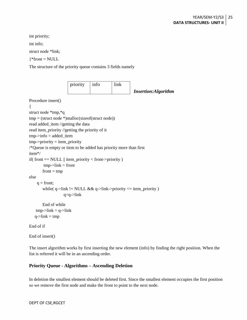
The structure of the priority queue contains 3 fields namely
Insertion:Algorithm
Procedure insert()
{
struct node *tmp,*q
tmp = (struct node *)malloc(sizeof(struct node))
read added_item //getting the data
read item_priority //getting the priority of it
tmp->info = added_item
tmp->priority = item_priority
/*Queue is empty or item to be added has priority more than first
item*/
if( front == NULL || item_priority < front->priority )
tmp->link = front
front = tmp
else
q = front;
while( q->link != NULL && q->link->priority <= item_priority )
q=q->link
End of while
tmp->link = q->link
q->link = tmp
End of if
End of insert()
The insert algorithm works by first inserting the new element (info) by finding the right position. When the
list is referred it will be in an ascending order.
Priority Queue - Algorithms – Ascending Deletion
In deletion the smallest element should be deleted first. Since the smallest element occupies the first position
so we remove the first node and make the front to point to the next node.
priority info link

YEAR/SEM-Y2/S3 DATA STRUCTURES- UNIT II
26
DEPT OF CSE,RGCET
Procedure ascen_del()
{
struct node *tmp;
if(front == NULL)
printf "Queue Underflow”
else
tmp = front;
front = front->link;
free(tmp);
End of if
End of procedure ascen_del()
Priority Queue - Algorithms – Descending Deletion
The last node will be having the highest priority value and its link will be NULL so we check for it and
delete the last node.
Procedure desc_del()
{
struct node *ptr,*prev;
if(front == NULL)
printf "Queue Underflow”
else
ptr = front;
while ( ptr->link!=NULL) do
prev=ptr
ptr=ptr->link
end while
prev->link=NULL
free(ptr);
YEAR/SEM-Y2/S3 DATA STRUCTURES- UNIT II
27
DEPT OF CSE,RGCET
End of if
End of procedure desc_del()
Run Time Complexity
Θ(lg n) time for Insert and worst case for deletion (where n is number of elements)
Θ(lg n) average time for Insert
Can construct a Heap from a list in Θ(lg n) where a Binary Search Tree takes Θ(n lg n)
Space Requirements
All operations are done in place - space requirement at any given time is the number of elements, n.
CIRCULAR QUEUE
In a standard queue data structure re-buffering problem occurs for each dequeue operation. To solve this
problem by joining the front and rear ends of a queue to make the queue as a circular queue
Circular queue is another form of a linear queue in which the last position is connected to the first
position of the list.
The circular queue is similar to linear queue has two ends, the front end and the rear end.
The rear end is where we insert the elements and the front end is where we delete the elements.
The traversing is in only one direction (i.e., from front to rear).
Initially the front and rear ends are at same position(i.e., -1);
While inserting elements the rear pointer moves one by one (where front pointer doesn’t change)
until the front end is reached.
If the next position of the rear is front, the queue is said to be fully occupied.
Beyond this insertion is not done.
But if we delete any data, we can insert the element accordingly.
While deleting the elements the front pointer moves one by one (where as the rear point doesn’t
change) until the rear point is reached.
If the front pointer reaches the rear pointer, both the ir positions are initialized to -1, and the queue is
said to be empty.
A more efficient queue representation is obtained by the circular array.
It becomes more convenient to declare the array as Q[n-1].
When rear = n-1, the next element is entered at Q[0] in case that position is free.

YEAR/SEM-Y2/S3 DATA STRUCTURES- UNIT II
28
DEPT OF CSE,RGCET
Using the same conventions, front will always point one position counterclockwise from the first
element in the queue.
Again, front=rear if and only if the queue is empty. Initially we have front = rear = 1.
The following figure illustrates some of the possible configurations for a circular queue containing
the four elements with n>4.
The assumption of circularity changes the ADD and DELETE algorithm slightly.
In order to add an element , it will be necessary to move rear one position clockwise, i.e.,
if rear = n-1 then rear =0
else rear = rear+1.
Using modulo operator which computes remainders, this is just rear=(rear+1)mod n.
Similarly, it will be necessary to move front one position clockwise each time a deletion is made.
Again, using the modulo operation, this can be accomplished by front=(front+1)mod n.
An examination of the algorithms indicates that addition and deletion can now be carried out in a
fixed amount of time or O(1).
Procedure ADDQ (item, Q, n, front, rear)
//insert item in the circular queue stored in Q (0: n-1);
rear points to the last item and front is one position counterclockwise from the first item in Q//
rear = (rear+1)mod n //advance rear clockwise//
if front = rear then call QUEUE-FULL
Q(rear)= item //insert new item //
end ADDQ.
Procedure DELETEQ (item, Q, n, front, rear)
//removes the front element of the queue Q (0: n-1)//
if front = rear then call QUEUE-EMPTY
front = (front + 1)mod n //advance front clockwise//
item = Q(front) //set item to front of queue//

YEAR/SEM-Y2/S3 DATA STRUCTURES- UNIT II
29
DEPT OF CSE,RGCET
end DELETEQ
Double Ended Queue (DEQUEUE)
Another variation of queue is known as dequeue. Unlike queue, in dequeue, both insertion and
deletion operations are made at either end of the structure ie, the element either at the front or rear
of the queue can be deleted and either the element can be added either at the front or at rear of the
queue.
Front rear
…………….
Algorithm
The implementation can be restricted into two ways
a) An input restricted dequeue which allows insertions at one end say Rear only, but
allows deletions at both ends
b) An output restricted dequeue where deletions take place at one end say front only but
allows insertions at both ends
Four possible operations are to take place.
Enqueue Left
Enqueue Right
Dequeue Left
Dequeue Right
For input restricted dequeue the operations are Enqueue Right, Dequeue Left, Dequeue Right.
For output restricted dequeue the operations are Enqueue Left, Enqueue Right, Dequeue Left.
Representing dequeue:
1. Double Linked List.
2. Circular Array.
Representing DEQUEUE using circular array - Algorithm
Procedure enqueueRight(int x)
{
if(q.rear==MAX)
printf("Queue full from Right\n");
else

YEAR/SEM-Y2/S3 DATA STRUCTURES- UNIT II
30
DEPT OF CSE,RGCET
{
q.x[++q.rear]=x;
if(q.front==-1)
q.front=0;
}
End of enqueueRight(int x)
procedure enqueueLeft(int x)
{
if(q.rear==-1 && q.front==-1)
enqueueRight(x);
else if(q.front==0)
printf("Queue full from Left\n");
else
{
q.x[--q.front]=x;
}
End of enqueueLeft(int x)
Procedure dequeueLeft()
{
int x;
if(q.rear==-1 && q.front==-1)
printf("Queue Empty\n");
else if(q.front==q.rear)
{
x=q.x[q.front];
q.front=q.rear=-1;
return x;
}else
return q.x[q.front++];
end of dequeueLeft()
procedure dequeueRight()
{
int x;
if(q.rear==-1 && q.front==-1)

YEAR/SEM-Y2/S3 DATA STRUCTURES- UNIT II
31
DEPT OF CSE,RGCET
printf("Queue Empty\n");
else if(q.front==q.rear)
{
x=q.x[q.front];
q.front=q.rear=-1;
return x;
}else
return q.x[q.rear--];
end of dequeueRight()
APPLICATIONS OF QUEUES
Numerous applications of queue structure are known in computer science. One major
application of queue is in simulation.
Another important application of queue is observed in implementation of various aspects of
operating system.
Multiprogramming environment uses several queues to control various programs.
And, of course, queues are very much useful to implement various algorithms. For example,
various scheduling algorithms are known to use varieties of queue structures.
General applications
There are several algorithms that use queues to give efficient running times.
When jobs are submitted to a printer, they are arranged in order of arrival. Thus,
essentially, jobs sent to a line printer are placed on a queue We say essentially a queue,
because jobs can be killed. This amounts to a deletion from the middle of the queue, which
is a violation of the strict definition.
Virtually every real-life line is (supposed to be) a queue. For instance, lines at ticket
counters are queues, because service is first-come first-served.
Another example concerns computer networks. There are many network setups of
personal computers in which the disk is attached to one machine, known as the file server.

YEAR/SEM-Y2/S3 DATA STRUCTURES- UNIT II
32
DEPT OF CSE,RGCET
Users on other machines are given access to files on a first-come first-served basis, so the
data structure is a queue.
Calls to large companies are generally placed on a queue when all operators are busy.
In large universities, where resources are limited, students must sign a waiting list if
all terminals are occupied. The student who has been at a terminal the longest is forced off
first, and the student who has been waiting the longest is the next user to be allowed on.
A whole branch of mathematics, known as queueing theory, deals with computing,
probabilistically, how long users expect to wait on a line, how long the line gets, and
other such questions. The answer depends on how frequently users arrive to the line and
how long it takes to process a user once the user is served. Both of these parameters are
given as probability distribution functions. In simple cases, an answer can be computed
analytically.
An example of an easy case would be a phone line with one operator. If the operator is
busy, callers are placed on a waiting line (up to some maximum limit). This problem is
important for businesses, because studies have shown that people are quick to hang up the
phone.
(a) Simulation
Simulation is a modeling of a real life problem, in other words, it is the model of a real life
Situation in the form of a computer program.
The main objective of the simulation program is to study the real life situation under the
control of various parameters which affect the real problem, and is a research interest of
system analysts or operation research scientists.
Based on the results of simulation, actual problem can be solved in an optimized way.
Another advantage of simulation is to experiment the danger area. for example, areas such
as military operations are safer to simulate than to field test, which is free from any risk as
well as inexpensive.
Simulation is a classical area where queries can be applied. Before going to discuss the
simulated modeling, let us study few terms related to it.

YEAR/SEM-Y2/S3 DATA STRUCTURES- UNIT II
33
DEPT OF CSE,RGCET
Any process or situation that is to be simulated is called a system. A system is a collection
of interconnected objects which accepts aero or more inputs and produces at least one
output, Figure(a).
For example, a computer program is a system where instructions are interconnected objects
and inputs or initialization values are the inputs and results during the execution is output.
Similarly, a ticket reservation counter is also a system. Note that a system can be composed
of one or more smaller system(s).
A system can be divided into different types as shown in Figure(b).
A system is discrete if the input/ output parameters are of discrete values.
For example, if customers arriving at a ticket reservation counter then it is a discrete
whereas water flowing through a pipe to a reservoir or emanating from it is an example of
continuous system; here the parameters are of continuous type.
A system is deterministic if from a given set of inputs and initial condition of the system,
final outcome can be predicted. For example, a program to calculate the factorial of an
integer is a deterministic system.
On the other hand, stochastic system is based on the randomness; its behavior cannot be
predicted before. As an another example, number of customers waiting in front of a ticket
YEAR/SEM-Y2/S3 DATA STRUCTURES- UNIT II
34
DEPT OF CSE,RGCET
reservation counter at any instant cannot be forecasted. There may be some systems which
are intermixing of both deterministic and stochastic.
After getting an idea about the variants type of systems.
Let us define various kind of simulation models.
There are two kind of simulation models: even-driven simulation and time-driven
simulation; these are decided by how the state of a system changes.
In case of time-driven simulation, systems change its states with the change of time and in
event-driven simulation, systems changes its state whenever a new event arrives to the
system or exits from the system.
Now let us consider a system, its model for simulation study and then application of queues
in it.
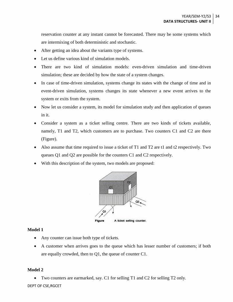
Consider a system as a ticket selling centre. There are two kinds of tickets available,
namely, T1 and T2, which customers are to purchase. Two counters C1 and C2 are there
(Figure).
Also assume that time required to issue a ticket of T1 and T2 are t1 and t2 respectively. Two
queues Q1 and Q2 are possible for the counters C1 and C2 respectively.
With this description of the system, two models are proposed:
Model 1
Any counter can issue both type of tickets.
A customer when arrives goes to the queue which has lesser number of customers; if both
are equally crowded, then to Q1, the queue of counter C1.
Model 2
Two counters are earmarked, say. C1 for selling T1 and C2 for selling T2 only.

YEAR/SEM-Y2/S3 DATA STRUCTURES- UNIT II
35
DEPT OF CSE,RGCET
A customer on arrival goes to either queue Q1 orQ2 depending on the ticket, that is,
Customer for T1 will be on Ql and that for T2 will be on Q2.
To simplify the simulation model, the underlying assumptions are made:
1. Queue lengths are infinite.
2. One customer in a queue is allowed for one ticket only. q
3. Let λ1 and λ2, are the mean arrival rates of customers for ticket T1 and 12
respectively. The values for λ1 and λ2 will be provided by the system analyst.
4. Let us consider the discrete probability distribution (also called poisson
distribution) for the arrival of the customers to the centre. Poisson distribution
gives a probability function
P(r) = l-e- λt
where P(r)= the probability that the next customer arrives at time t. and /1=the mean
arrival rate. Thus, if we assume N be the total population of customers in a day, then
N1= N1P(t) = N1 (l-e- λ1
t)
is the number of customers arrived at the centre for ticket T1 at time t and N2= N2P(t) = N2
(l-e- λ2
t), is the number of customers arrived the centre for ticket T2 at time t.
5. A clock is maintained with an initial value (to dictate the opening and closing of
counters, when the counter is made available to the customer, etc.
With the these assumptions, the objective of the simulation model is to study the
performance of the system under various conditions.
Average queuing time
It is defined as the average time that a customer for a ticket Ti (i = 1, 2) will be in queue
(this time includes service time Ti (i = 1, 2). that is, the time to issue a ticket).
Average queue length
It is the average length of the queue Qi (i = 1, 2) over a day.
Total service time

YEAR/SEM-Y2/S3 DATA STRUCTURES- UNIT II
36
DEPT OF CSE,RGCET
It is the time that a counter Ci(i= 1,2) remains busy over a day.
With these basic assumptions and definition, the proposed simulation model may be termed
as discrete deterministic time-driven simulation model.
(b) CPU scheduling in multiprogramming environment
In a multiprogramming environment, a single CPU has to serve more than one program
simultaneously.
Consider a multiprogramming environment where possible jobs to the CPU are categorized
into three groups:
1. Interrupts to be serviced. Variety of devices and terminals are connected with the CPU
and they may interrupt at any moment to get a service from it.
2. Interactive users to be serviced. These are mainly student's programs in various
terminals under execution.
3. Batch jobs to be serviced.
These are long term jobs mainly from the non-interactive users, where all the inputs are fed
when jobs are submitted; simulation programs, and jobs to print documents are of this kind.
Here the problem is to schedule all sorts of jobs so that the required level of performance of
the environment will be attained.
One way to implement complex scheduling is to classify the work load according to its
characteristics and t o maintain separate process queues.
So far the environment is concerned, we can maintain three queues, as depicted in Figure.
YEAR/SEM-Y2/S3 DATA STRUCTURES- UNIT II
37
DEPT OF CSE,RGCET
This approach is often called multi-level queues scheduling. Process will be assigned to
their respective queues.
CPU will then service the processes as per the priority of the queues. In case of a simple
strategy, absolute priority, the process from the highest priority queue (for example, system
processes) are serviced until the queue becomes empty.
Then CPU switches to the queue of interactive processes which is having medium-priority
and so on.
A lower- priority process may, of course. be pre-empted by a higher-priority arrival in one
of the upper- level queues.
Multi-level queues strategy is a general discipline but has some drawbacks. The main
drawback is that when process arrived in higher-priority queues is very high.
The processes in lower-priority queue may starve for a long time.
One way out to solve this problem is to time slice between the queues. Bach queue gets a
certain portion of the CPU time.
Another possibility is known as multi-level feedback queue strategy. Normally in multi-
level queue strategy, processes are permanently assigned to a queue upon entry to the
system and processes do not move among queues.
Multi-level feedback queue strategy, on the contrary, allows a process to move between
queues. The idea is to separate out processes with different CPU burst characteristics.
If a process uses too much CPU time (that is long run process), it will be moved to a lower-
priority queue.
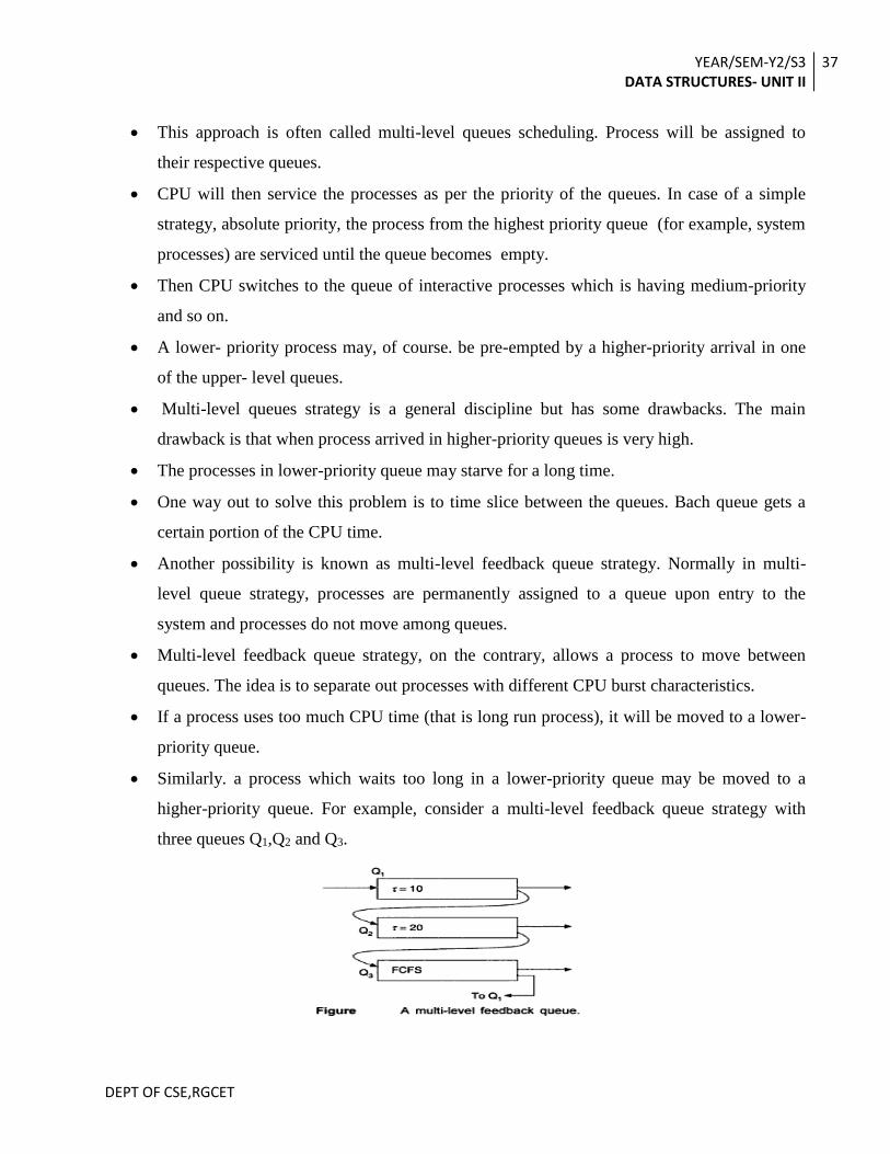
Similarly. a process which waits too long in a lower-priority queue may be moved to a
higher-priority queue. For example, consider a multi-level feedback queue strategy with
three queues Q1,Q2 and Q3.

YEAR/SEM-Y2/S3 DATA STRUCTURES- UNIT II
38
DEPT OF CSE,RGCET
A process entering the system is put in queue Q1. A process in Q1 is given a time quantum τ
of I0 ms, say, it does not finish within this time, it is moved to the tail of queue Q2.
If Q1 is empty, the process at the front of queue Q2 is given a time quantum τ of 20 ms, say.
If it does not complete within this time quantum. it is pre-empted and put into queue Q3.
Processes in queue Q3 are serviced only when queues Q1 and Q2 are empty.
Thus, with this strategy, CPU first executes all processes in queue Q1.
Only when Q1 is empty it will execute all processes in queue Q2. Similarly, processes in
queue Q3 will only be executed if queues Q1 and Q2 are empty.
A process which arrives in queue Q1 will pre-empt a process in queue Q2 or Q3.
lt can be observed that, this strategy gives the highest priority to any process with a CPU
burst of 10 ms or less. Processes which need more than 10 ms. but less than or equal to 20
ms are also served quickly, that is, it gets the next highest priority than the shorter processes.
Longer processes automatically sink to queue Q3, from Q3. Processes will be served in first-
come first-serve (FCFS) basis and in case of process waiting for a too long time (as decided
by the scheduler) may be put into the tail of queue Q1.
(c) Round Robin Algorithm
Round robin (RR) algorithm is a well-known scheduling algorithm and is designed
especially for time sharing systems.
A circular queue can be used to implement such an algorithm.
Suppose, there are n processes P1, P2, . . .. Pn, required to be served by the CPU.
Different processes require different execution time. Suppose, sequence of process arrivals
are according to their subscripts, that is. P1 comes first than P2 and in general, Pi comes after
Pi-1 for 1 < i ≤ n.
RR algorithm first decides a small unit of time, called a time quantum or time slice, τ.
A time quantum is generally from I0 to l00 milliseconds. CPU starts services with P1. P1
gets CPU for τ instant of time.
Afterwards CPU switches to P2 and so on. When CPU reaches the end of time quantum of
Pn it returns to P1 and the same process will be repeated.

YEAR/SEM-Y2/S3 DATA STRUCTURES- UNIT II
39
DEPT OF CSE,RGCET
Now, during time sharing, if a process finishes its execution before the finishing of its time
quantum, the process then simply releases the CPU and the next process waiting will get
the CPU immediately.
The advantages of this kind of scheduling is reducing the average turnaround time (not
necessarily true always). Turn around time of a process is the time of its completion - time
of its arrival.
In time sharing systems any process may arrive at any instant of time.
Generally, all the process currently under executions, are maintained in a queue. When a
process finishes
Implementation of RR scheduling algorithm. Circular queue is the best choice for it. If
may be noted that it is not strictly a circular queue because here a process when it completes
its execution required to be deleted from the queue and it is not necessarily from the front of
the queue rather from any position of the queue.
Except this, it follows all the properties of queue, that is, processes which comes first gets
its turn first.
Implementation of the RR algorithm using a circular queue is straightforward.
Variable sized circular queue is used; size of the queue at any instant is decided by the
number of processes in execution at that instant.
Another mechanism is necessary; whenever a process is deleted, to fill the space of deleted
process, it is required to squeeze ell the processes preceding to it starting from the front
pointer.
YEAR/SEM-Y2/S3 DATA STRUCTURES- UNIT II
40
DEPT OF CSE,RGCET
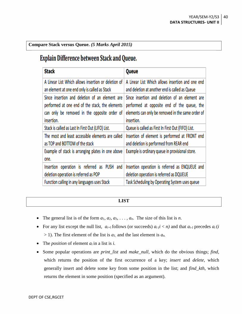
Compare Stack versus Queue. (5 Marks April 2015)
LIST
The general list is of the form a1, a2, a3, . . . , an. The size of this list is n.
For any list except the null list, ai+l follows (or succeeds) ai (i < n) and that ai-1 precedes ai (i
> 1). The first element of the list is a1, and the last element is an.
The position of element ai in a list is i.
Some popular operations are print_list and make_null, which do the obvious things; find,
which returns the position of the first occurrence of a key; insert and delete, which
generally insert and delete some key from some position in the list; and find_kth, which
returns the element in some position (specified as an argument).

YEAR/SEM-Y2/S3 DATA STRUCTURES- UNIT II
41
DEPT OF CSE,RGCET
If the list is 34, 12, 52, 16, 12, then find(52) might return 3; insert(x,3) might makes the list
into 34, 12, 52, x, 16, 12 (if we insert after the position given); and delete(3) might turn that
list into 34, 12, x, 16, 12.
Simple Array Implementation of Lists
Obviously all of these instructions can be implemented just by using an array. Even if the
array is dynamically allocated, an estimate of the maximum size of the list is required.
Usually this requires a high over-estimate, which wastes considerable space. This could
be a serious limitation, especially if there are many lists of unknown size.
An array implementation allows print_list and find to be carried out in linear time, which is
as good as can be expected, and the find_kth operation takes constant time. However,
insertion and deletion are expensive. For example, inserting at position 0 (which
amounts to making a new first element) requires first pushing the entire array down
one spot to make room, whereas deleting the first element requires shifting all the
elements in the list up one, so the worst case of these operations is O(n). On average,
half the list needs to be moved for either operation, so linear time is still required. Merely
building a list by n successive inserts would require quadratic time.
Because the running time for insertions and deletions is so slow and the list size must
be known in advance, simple arrays are generally not used to implement lists.
Comparison of Methods
Which is the best? A pointer-based or array-based implementation of lists. Often the answer
depends on which operations intended to perform, or on which are performed most frequently.
Other times, the decision rests on how long the list is likely to get. The principal issues to consider
are the following.
1. The array implementation requires us to specify the maximum size of a list at compile time.
If a bound cannot be put on the length to which the list will grow, probably choose a
pointer-based implementation.
2. Certain operations take longer in one implementation than the other. For example, INSERT
and DELETE take a constant number of steps for a linked list, but require time proportional
to the number of following elements when the array implementation is used. Conversely,

YEAR/SEM-Y2/S3 DATA STRUCTURES- UNIT II
42
DEPT OF CSE,RGCET
executing PREVIOUS and END require constant time with the array implementation, but
time proportional to the length of the list if pointers are used.
3. If a program calls for insertions or deletions that affect the element at the position denoted
by some position variable, and the value of that variable will be used later on, then the
pointer representation cannot be used. As a general principle, pointers should be used with
great care and restraint.
4. The array implementation may waste space, since it uses the maximum, amount of space
independent of the number of elements actually on the list at any time. The pointer
implementation uses only as much space as is needed for the elements currently on the list,
but requires space for the pointer in each cell. Thus, either method could wind up using
more space than the other in differing circumstances.
LINKED LISTS
Explain in detail about any two types of linked list with a neat diagram. (11 Marks April 2015)
Linked list is a data structure in which each data item points to the next data item. This "linking" is accomplished by keeping an address variable (a pointer) together with each data item. This pointer is used to store the address of the next data item in the list. The structure that is used to store one element of a linked list is called a node. A node has two parts: data and next address. The data part contains the necessary information about the items of the list, the next address part contains the address of the next node.
YEAR/SEM-Y2/S3 DATA STRUCTURES- UNIT II
43
DEPT OF CSE,RGCET
SINGLE LINKED LIST
Write an algorithm to insert a node at the first and middle and delete a node at the end of a
linked list. (11 Marks April 2012)
Write routines to insert and delete an element in single linked list. Explain with examples.
(11 Marks April 2015)
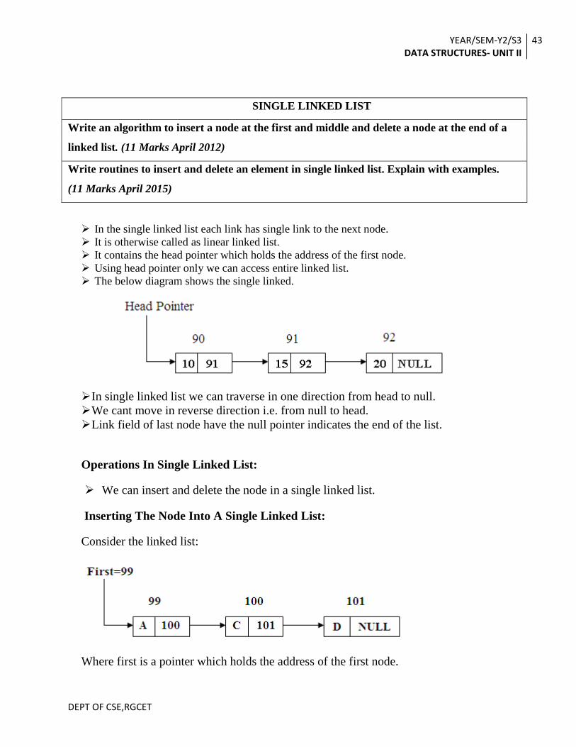
In the single linked list each link has single link to the next node.
It is otherwise called as linear linked list.
It contains the head pointer which holds the address of the first node.
Using head pointer only we can access entire linked list.
The below diagram shows the single linked.
In single linked list we can traverse in one direction from head to null.
We cant move in reverse direction i.e. from null to head.
Link field of last node have the null pointer indicates the end of the list.
Operations In Single Linked List:
We can insert and delete the node in a single linked list.
Inserting The Node Into A Single Linked List:
Consider the linked list:
Where first is a pointer which holds the address of the first node.

YEAR/SEM-Y2/S3 DATA STRUCTURES- UNIT II
44
DEPT OF CSE,RGCET
If we want to insert a data B , into the list , first we need the empty node with empty data
and link field.
Consider x is the address of new node.
Now put the data B into the data field of a new node and put NULL into the link field.
We can insert the new node by any one of the following position:
1. As a first node
2. As a intermediate node
3. As a last node.
Inserting as a first node:
If we want to insert a new node as a first node, the link field of new node is replaced by
FIRST and FISRT is replaced by X as shown below.
Inserting as a last node:
If we want to insert a node as a last node, the link field of new node is replaced by NULL
and the link field of last but previous link field is replaced by X as shown below.

YEAR/SEM-Y2/S3 DATA STRUCTURES- UNIT II
45
DEPT OF CSE,RGCET
Inserting as an intermediate node:
If we want to insert a new node as the intermediate node, first we need the address of
the previous node.
Now insert the new node in between the respective node as shown below
If we want to insert a new node X as intermediate node, insert in between C and D.
The link field of 99 is 100, the link field of 100 is 101 and the link field of 101 is 102.
Structure Definition
typedef struct node *node_ptr;
struct node
{
element_type element;
node_ptr next;
};
typedef node_ptr list;
typedef node_ptr position;
Empty list with header
Function to test whether a linked list is empty
The function is_empty () makes the L->next ( L is the header) to point to null in case the list
is empty.
int is_empty( list L)
{
YEAR/SEM-Y2/S3 DATA STRUCTURES- UNIT II
46
DEPT OF CSE,RGCET
return( L->next == null );
}
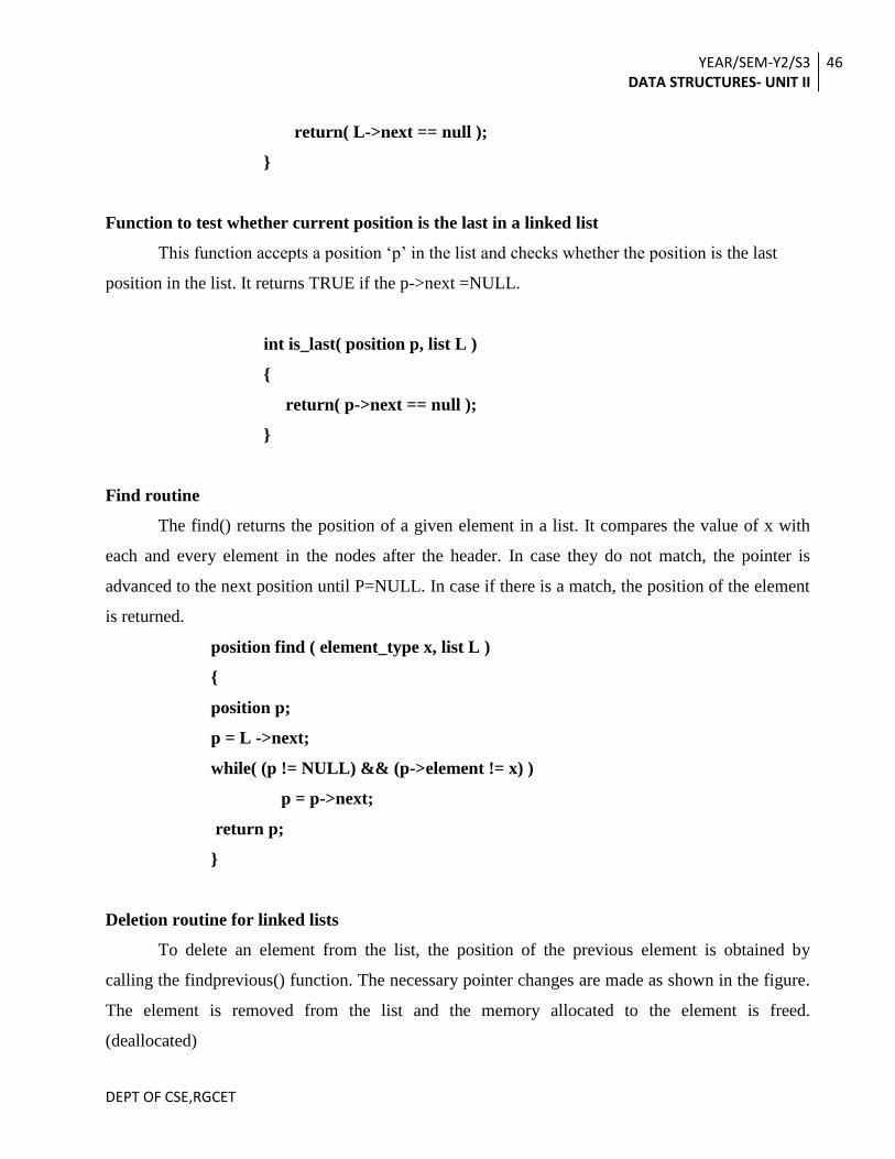
Function to test whether current position is the last in a linked list
This function accepts a position ‘p’ in the list and checks whether the position is the last
position in the list. It returns TRUE if the p->next =NULL.
int is_last( position p, list L )
{
return( p->next == null );
}
Find routine
The find() returns the position of a given element in a list. It compares the value of x with
each and every element in the nodes after the header. In case they do not match, the pointer is
advanced to the next position until P=NULL. In case if there is a match, the position of the element
is returned.
position find ( element_type x, list L )
{
position p;
p = L ->next;
while( (p != NULL) && (p->element != x) )
p = p->next;
return p;
}
Deletion routine for linked lists
To delete an element from the list, the position of the previous element is obtained by
calling the findprevious() function. The necessary pointer changes are made as shown in the figure.
The element is removed from the list and the memory allocated to the element is freed.
(deallocated)

YEAR/SEM-Y2/S3 DATA STRUCTURES- UNIT II
47
DEPT OF CSE,RGCET
void delete( element_type x, list L )
{
position p, tmp_cell;
p = find_previous( x, L );
if( p->next != null )
{ /* x is found: delete it */
tmp_cell = p->next;
p->next = tmp_cell->next;
free( tmp_cell );
}
}
Find_previous - the find routine for use with delete
The find_previous() returns the position of the previous element in a list. It compares the
value of x with each and every element in the nodes after the header. In case they do not match, the
pointer is advanced to the next position until p=NULL. In case if there is a match, the position of
the previous element is returned.
position find_previous( element_type x, list L )
{
position p;
/*1*/ p = L;
/*2*/ while( (p->next != NULL) && (p->next->element != x) )
/*3*/ p = p->next;
/*4*/ return p;
}
Insertion routine for linked lists
To insert an element into the list, the position after which the element is to be inserted
should be provided. To insert an element, memory is allocated using malloc. The necessary pointer
changes are made as shown in the figure.
YEAR/SEM-Y2/S3 DATA STRUCTURES- UNIT II
48
DEPT OF CSE,RGCET
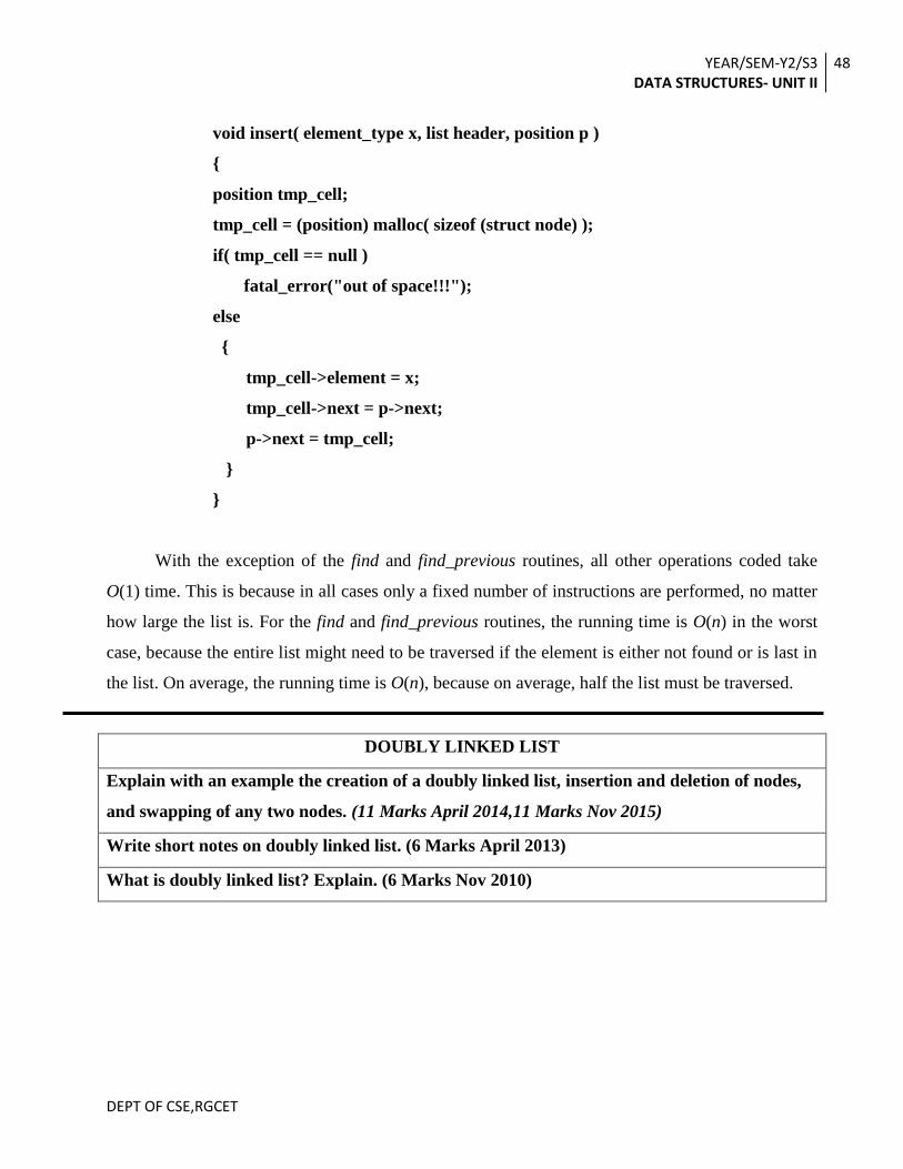
void insert( element_type x, list header, position p )
{
position tmp_cell;
tmp_cell = (position) malloc( sizeof (struct node) );
if( tmp_cell == null )
fatal_error("out of space!!!");
else
{
tmp_cell->element = x;
tmp_cell->next = p->next;
p->next = tmp_cell;
}
}
With the exception of the find and find_previous routines, all other operations coded take
O(1) time. This is because in all cases only a fixed number of instructions are performed, no matter
how large the list is. For the find and find_previous routines, the running time is O(n) in the worst
case, because the entire list might need to be traversed if the element is either not found or is last in
the list. On average, the running time is O(n), because on average, half the list must be traversed.
DOUBLY LINKED LIST
Explain with an example the creation of a doubly linked list, insertion and deletion of nodes,
and swapping of any two nodes. (11 Marks April 2014,11 Marks Nov 2015)
Write short notes on doubly linked list. (6 Marks April 2013)
What is doubly linked list? Explain. (6 Marks Nov 2010)
YEAR/SEM-Y2/S3 DATA STRUCTURES- UNIT II
49
DEPT OF CSE,RGCET

YEAR/SEM-Y2/S3 DATA STRUCTURES- UNIT II
50
DEPT OF CSE,RGCET
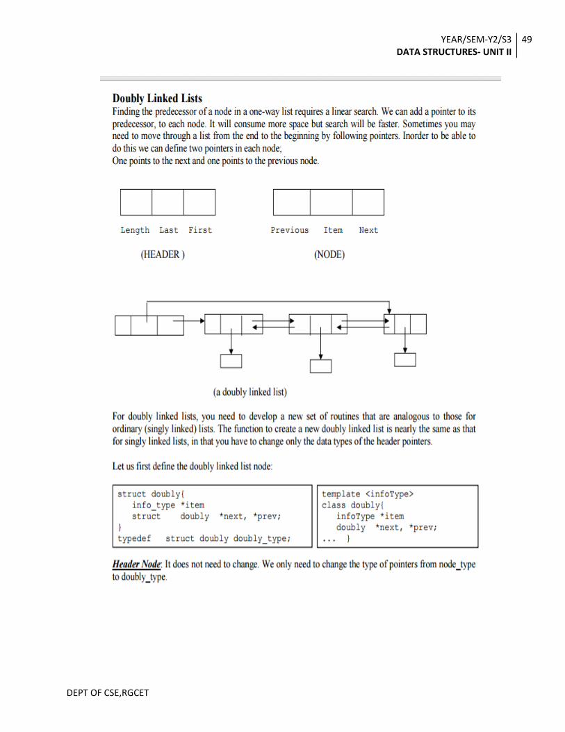
It is convenient to traverse lists backwards. Add an extra field to the data structure,
containing a pointer to the previous cell. The cost of this is an extra link, adds to the space
requirement and also doubles the cost of insertions and deletions because there are more
pointers to fix.
On the other hand, it simplifies deletion, because you no longer have to refer to a key by
using a pointer to the previous cell; this information is now at hand. Figure shows a doubly
linked list.
Structure Definition
Each node contains three fields. First field is data and there are two pointers next and previous.
Struct node
{
elementtype element;
ptrtonode *next,*previous;
};
typedef node_ptr list;
Function to check whether the list is empty or not
The function is_empty () makes the header->next to point to null in case if the list is empty.
int is_empty(list L)
{
return(L->next==NULL);
error(“List is empty”);
}
Function to check whether the element is in the last position
This function accepts a position P in the list and checks whether the position is the last
position in the list. It returns TRUE if the P->next =NULL.
int is_last (List L, position P)
{
return(P->next==NULL);
}

YEAR/SEM-Y2/S3 DATA STRUCTURES- UNIT II
51
DEPT OF CSE,RGCET
Find the position of the element
The find() returns the position of a given element in a list. It compares the value of x with
each and every element in the nodes after the header. In case they do not match, the pointer is
advanced to the next position until P=NULL. In case if there is a match, the position of the element
is returned.
position find(element type x, list L)
{
Position P;
P=L->next;
while (P!=NULL && P->element!=X)
P=P->next;
return P;
}
Find the position of the previous element
The findprevious() returns the position of the previous element in a list. It compares the
value of x with each and every element in the nodes after the header. In case they do not match, the
pointer is advanced to the next position until P=NULL. In case if there is a match, the position of
the previous element is returned.
position find previous(element type X, list L)
{
Position P;
P=L;
while(P->next!=NULL&&P->next->element!=X)
{
P=P->next;
return;
}
}
Find the position of the next element
YEAR/SEM-Y2/S3 DATA STRUCTURES- UNIT II
52
DEPT OF CSE,RGCET
The findnext() returns the position of the next element in a list. It compares the value of x
with each and every element in the nodes after the header. In case they do not match, the pointer is
advanced to the next position until P=NULL. In case if there is a match, the position of the next
element is returned.
position findnext (element type x, list L)
{
position P;
P=L;
while(P->next!=NULL && P->next->element!=x)
{
P=P->next;
}
return P->next;
}
Insert an element
To insert an element into the list, the position after which the element is to be inserted
ahould be provided. To insert an element, memory is allocated using malloc. The necessary pointer
changes are made as shown in the figure.
void insert(element type X, list L, position P)
{
Position tempcell;
tempcell=malloc(sizeof(struct node));
if(tempcell==NULL)
error(“Tempcell is empty”);
tempcell->element=X;
tempcell->next=P->next;
P->next=tempcell;
tempcell->next->prev=tempcell;
tempcell->prev=P;
}

YEAR/SEM-Y2/S3 DATA STRUCTURES- UNIT II
53
DEPT OF CSE,RGCET
Delete
To delete an elemnt from the list, the position of the previous element is obtained by calling
the findprevious() function. The necessary pointer changes are made as shown in the figure. The
element is removed from the list and the memory allocated to the element is freed. (deallocated)
void delete(element type X, list L)
{
Position P, tempcell;
P=Find previous(X,L);
if(!islast(P,L))
{
tempcell =P->next;
tempcell ->next->prev = p;
P->next=tempcell->next;
Free(tempcell);
}
CIRCULAR LINKED LIST 11 Marks Nov 2015
A popular convention is to have the last cell keep a pointer back to the first. This can be done
with or without a header (if the header is present, the last cell points to it), and can also be
done with doubly linked lists (the first cell's previous pointer points to the last cell).
The next pointer of the last element points to the header, if the header is present. If not, it
simply points to the first element.
Structure Definition
Each node contains two fields. Every last node points the header.
Struct node
{

YEAR/SEM-Y2/S3 DATA STRUCTURES- UNIT II
54
DEPT OF CSE,RGCET
Element type element;
Position next;
};
typedef node_ptr list;
list L;
L->next=L; // // L is the header.
Function to check whether the list is empty or not
The function is_empty() makes the L->next to point to L in case if the list is empty.
int is_empty (list L)
{
return L->next==L;
}
Function to check whether the element is in the last position
This function accepts a position P in the list and checks whether the position is the last
position in the list. It returns TRUE if the P->next =L.
int is_last(position P, List L)
{
return P->next==L;
}
Find the position of the element
The find() returns the position of a given element in a list. It compares the value of x with
each and every element in the nodes after the header. In case they do not match, the pointer is
advanced to the next position until P=L, the header. In case if there is a match, the position of the
element is returned.
position find(Element type x, List L)
{
Position P;
P=L->next;
while(P!=L && P->element!=X)

YEAR/SEM-Y2/S3 DATA STRUCTURES- UNIT II
55
DEPT OF CSE,RGCET
P=P->next;
return P;
}
Find the position of the previous element
The findprevious() returns the position of the previous element in a list. It compares the
value of x with each and every element in the nodes after the header. In case they do not match, the
pointer is advanced to the next position until P=HEADER. In case if there is a match, the position
of the previous element is returned.
position findprevious (Element type X, List L)
{
Position P;
P=L;
while(P->next==L && P->next->element!=X)
P=P->next;
return P;
}
Insert
To insert an element into the list, the position after which the element is to be inserted
ahould be provided. To insert an element, memory is allocated using malloc. The necessary pointer
changes are made as shown in the figure.
void insert(Element typeX,List L,position P)
{
position P,tempcell;
Tempcell=malloc(sizeof(struct node));
if(tempcell=NULL)
Error(“Out of space”);
Tempcell->Element=x;
Tempcell->next=P->next;
P->next=tempcell;
YEAR/SEM-Y2/S3 DATA STRUCTURES- UNIT II
56
DEPT OF CSE,RGCET
}
Delete
To delete an element from the list, the position of the previous element is obtained by
calling the findprevious() function. The necessary pointer changes are made as shown in the figure.
void delete(Element type X, List L)
{
Position P,Tempcell;
P=findprevious(X,L);
if(!is last(P,L))
{
Tempcell=P->next;
P->next=tempcell->next;
free(tempcell);
}
}
APPLICATIONS OF A LIST
In order to store and process data, linked list are very popular data structures.
This type of data structures holds certain advantages over arrays.
Demerits of arrays and Merits of linked lists
First, in case of an array, data are stored in contiguous memory locations, so insertion and
deletion operations are quite time consuming, in insertion of a new element at a desired
location , all the trailing elements should be shifted down; similarly, in case of deletion, in
order to fill the location of deleted element, all the trailing elements are required to shift
upwards. But, in linked lists, it is a matter of only change in pointers.
Second, array is based on the static allocation of memory: amount of memory required
for an array must be known before hand, once it is allocated its size cannot be expanded.
This is why, for an array, general practice is to allocate memory, which is much more than

YEAR/SEM-Y2/S3 DATA STRUCTURES- UNIT II
57
DEPT OF CSE,RGCET
the memory that actually will be used. But this is simply wastage of memory space. This
problem is not there in linked list. Linked list uses dynamic memory management
scheme; memory allocation is decided during the run-time as and when require. Also if a
memory is no more required, it can be returned to the free storage space, so that other
module or program can utilize it.
Third, a program using an array may not execute although the memory required for the data
are available but not in contiguous locations rather dispersed. As link structures do not
necessarily require to store data in adjacent memory location, so the program of that kind,
using linked list can then be executed.
Demerits of linked lists
However, there are obviously some disadvantages: one is the pointer business. Pointers, if
not managed carefully, may lead to serious errors in execution.
Next, linked lists consume extra space than the space for actual data as the links among the
nodes are to be maintained.
Five examples are provided that use linked lists.
The first is a simple way to represent single-variable polynomials.
The second is a method to sort in linear time, for some special cases.
Thirdly, linked lists might be used to keep track of course registration at a university.
The next application is the representation of sparse matrix
The last application is Dynamic Storage management
The Polynomial ADT
An abstract data type for single-variable polynomials (with nonnegative exponents) can be
defined by using a list.
If most of the coefficients ai are nonzero, use a simple array to store the coefficients.
Routines can be written to perform addition, subtraction, multiplication, differentiation, and
other operations on these polynomials. In this case, use the type declarations below.
Two possibilities are addition and multiplication.
YEAR/SEM-Y2/S3 DATA STRUCTURES- UNIT II
58
DEPT OF CSE,RGCET
Ignoring the time to initialize the output polynomials to zero, the running time of the
multiplication routine is proportional to the product of the degree of the two input
polynomials. This is adequate for dense polynomials, where most of the terms are present,
but if p1(x) = 10x1000 + 5x14 + 1 and p2(x) = 3x1990 - 2x1492 + 11x + 5, then the running time is
likely to be unacceptable.
Most of the time is spent multiplying zeros and stepping through what amounts to
nonexistent parts of the input polynomials. This is always undesirable.
typedef struct
{
int coeff_array[ MAX_DEGREE+1 ];
unsigned int high_power;
} *POLYNOMIAL;
Type declarations for array implementation of the polynomial ADT
An alternative is to use a singly linked list. Each term in the polynomial is contained in one
cell, and the cells are sorted in decreasing order of exponents. For instance, the linked lists
in represent p1(x) and p2(x).
void zero_polynomial( POLYNOMIAL poly )
{
unsigned int i;
for( i=0; i<=MAX_DEGREE; i++ )
poly->coeff_array[i] = 0;
poly->high_power = 0;
}
Procedure to initialize a polynomial to zero
void add_polynomial( POLYNOMIAL poly1, POLYNOMIAL poly2,
POLYNOMIAL poly_sum )
{

YEAR/SEM-Y2/S3 DATA STRUCTURES- UNIT II
59
DEPT OF CSE,RGCET
int i;
zero_polynomial( poly_sum );
poly_sum->high_power = max( poly1->high_power,
poly2->high_power);
for( i=poly_sum->high_power; i>=0; i-- )
poly_sum->coeff_array[i] = poly1->coeff_array[i] + poly2-
>coeff_array[i];
}
Procedure to add two polynomials
void mult_polynomial( POLYNOMIAL poly1, POLYNOMIAL poly2, POLYNOMIAL
poly_prod )
{
unsigned int i, j;
zero_polynomial( poly_prod );
poly_prod->high_power = poly1->high_power + poly2->high_power;
if( poly_prod->high_power > MAX_DEGREE )
error("Exceeded array size");
else
for( i=0; i<=poly->high_power; i++ )
for( j=0; j<=poly2->high_power; j++ )
poly_prod->coeff_array[i+j] += poly1->coeff_array[i] * poly2->coeff_array[j];
}
Procedure to multiply two polynomials
Linked list representations of two polynomials

YEAR/SEM-Y2/S3 DATA STRUCTURES- UNIT II
60
DEPT OF CSE,RGCET
typedef struct node *node_ptr;
struct node
{
int coefficient;
int exponent;
node_ptr next;
} ;
typedef node_ptr POLYNOMIAL; /* keep nodes sorted by exponent */
Type declaration for linked list implementation of the Polynomial ADT
The operations would then be straightforward to implement. The only potential difficulty is
that when two polynomials are multiplied, the resultant polynomial will have to have like terms
combined.
Multilists
Last example shows a more complicated use of linked lists. A university with 40,000
students and 2,500 courses needs to be able to generate two types of reports. The first report
lists the class registration for each class, and the second report lists, by student, the classes
that each student is registered for.
The obvious implementation might be to use a two-dimensional array. Such an array would
have 100 million entries. The average student registers for about three courses, so only
120,000 of these entries, or roughly 0.1 percent, would actually have meaningful data.
What is needed is a list for each class, which contains the students in the class. A list for
each student is also needed, which contains the classes the student is registered for.

YEAR/SEM-Y2/S3 DATA STRUCTURES- UNIT II
61
DEPT OF CSE,RGCET
Multilist implementation for registration problem
As the figure shows, two lists are combined into one. All lists use a header and are circular.
To list all of the students in class C3, start at C3 and traverse its list (by going right).
The first cell belongs to student S1. Although there is no explicit information to this effect,
this can be determined by following the student's linked list until the header is reached.
Once this is done, return to C3's and find another cell, which can be determined to belong to
S3. Continue and find that S4 and S5 are also in this class. In a similar manner, for any
student, all of the classes in which the student is registered can be determined.
Sparse Matrix Manipulation
Linked lists are the best solution to store them.
The node structure to represent any sparse matrix is shown in the Figure.
In the Figure, fields i and j store the row and column numbers for a matrix element
respectively.
DATA field stores the matrix element at the i-th row and the j-th column, i.e., aij.
The ROWLINK points to the next node in the same row and COLLINK points the next
node in the same column.
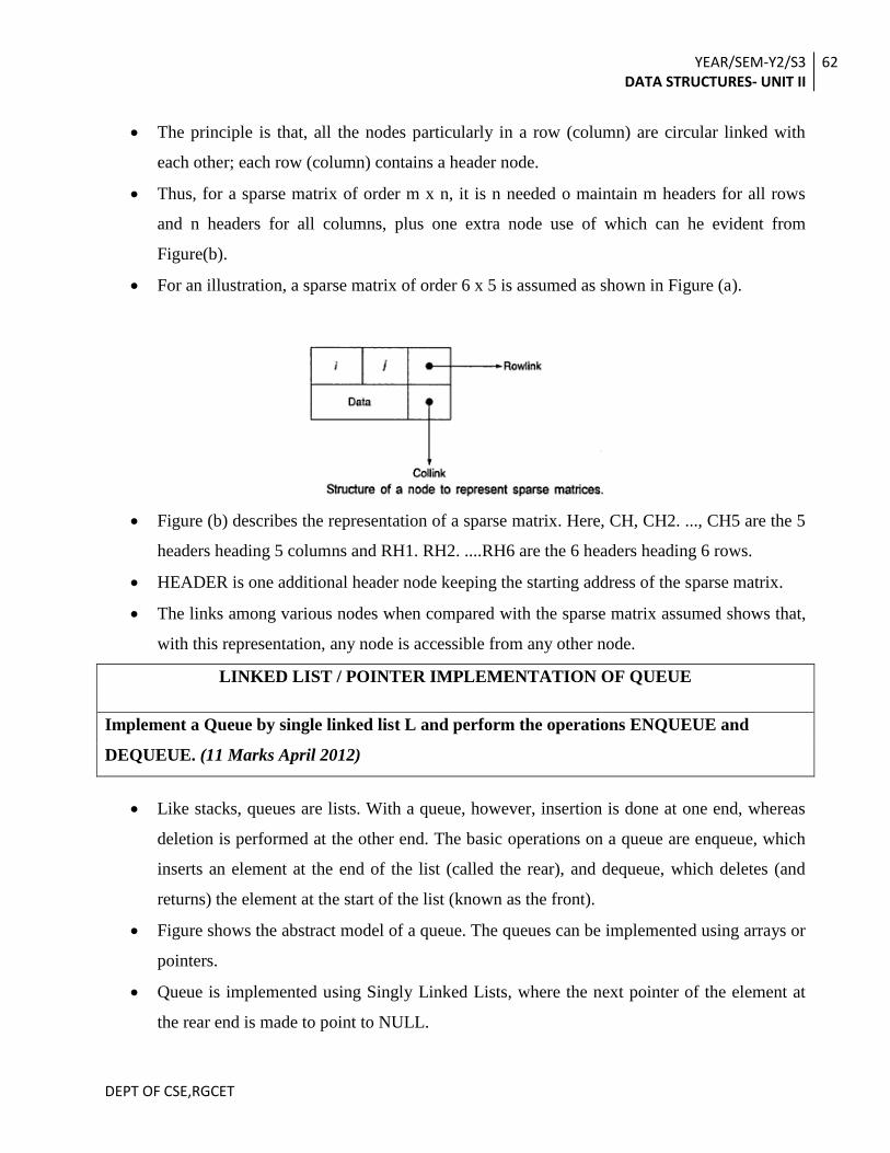
YEAR/SEM-Y2/S3 DATA STRUCTURES- UNIT II
62
DEPT OF CSE,RGCET
The principle is that, all the nodes particularly in a row (column) are circular linked with
each other; each row (column) contains a header node.
Thus, for a sparse matrix of order m x n, it is n needed o maintain m headers for all rows
and n headers for all columns, plus one extra node use of which can he evident from
Figure(b).
For an illustration, a sparse matrix of order 6 x 5 is assumed as shown in Figure (a).
Figure (b) describes the representation of a sparse matrix. Here, CH, CH2. ..., CH5 are the 5
headers heading 5 columns and RH1. RH2. ....RH6 are the 6 headers heading 6 rows.
HEADER is one additional header node keeping the starting address of the sparse matrix.
The links among various nodes when compared with the sparse matrix assumed shows that,
with this representation, any node is accessible from any other node.
LINKED LIST / POINTER IMPLEMENTATION OF QUEUE
Implement a Queue by single linked list L and perform the operations ENQUEUE and
DEQUEUE. (11 Marks April 2012)
Like stacks, queues are lists. With a queue, however, insertion is done at one end, whereas
deletion is performed at the other end. The basic operations on a queue are enqueue, which
inserts an element at the end of the list (called the rear), and dequeue, which deletes (and
returns) the element at the start of the list (known as the front).
Figure shows the abstract model of a queue. The queues can be implemented using arrays or
pointers.
Queue is implemented using Singly Linked Lists, where the next pointer of the element at
the rear end is made to point to NULL.

YEAR/SEM-Y2/S3 DATA STRUCTURES- UNIT II
63
DEPT OF CSE,RGCET
Queue Model
The basic operations on a queue are enqueue, which inserts an element at the end of the list
(called the rear), and dequeue, which deletes (and returns) the element at the start of the list (known
as the front). Figure shows the abstract model of a queue.
Structure definition
Each node contains two fields. Every last node points to null.
Struct node
{
element type element ;
ptr to node*next;
};
typedef node_ptr queue;
Function to check whether the queue is empty or not
This function is empty checks whether the queue is empty or not, It returns true, if the queue
is empty. It makes the q->next to point to NULL in case if the queue is empty.
int is_Empty (queue q)
{
return q->next= = NULL;
}
Creating a Queue
It allocates memory for the given structure (header of the queue. It points to the element at
the front of the queue). The queue is emptied by calling makeempty( ) function.
queue create queue (void)
{
queue q;
q=malloc (sizeof(struct node));
if(q= = null)
fatal error(“OUT OF SPACE”):
make empty(q);
return q;
}

YEAR/SEM-Y2/S3 DATA STRUCTURES- UNIT II
64
DEPT OF CSE,RGCET
Function to empty the queue
If the queue is not empty, the elements in the queue are removed until the queue becomes
empty. In other words, the queue exists but the queue is empty.
void make empty(queue q)
{
if(q = =null)
error(“Must use create queue first”);
else
while(!isempty (q));
delete(q);
}
Function to insert an element into the queue
To insert an element into the queue, in the linked list implementation, it is possible only at
the rear end. Therefore the position of the last element (p) is found. The last element’s next pointer
points to NULL.
void insert (elementtype X, queue q)
{
ptr tonode tempcell;
p=q;
tempcell=malloc(sizeof (struct node));
if(tempcell==NULL)
fatalerror(“out of space”);
else
{
while (p->next!=NULL)
p=p->next;
tempcell->element=X;
tempcell->next=p->next;
p->next=tempcell;
}
YEAR/SEM-Y2/S3 DATA STRUCTURES- UNIT II
65
DEPT OF CSE,RGCET
}
Function to return the first element in the list
It checks whether the queue is empty. If it is not empty, it returns the element at the front of
the queue
int front(queue q)
{
if(!isempty (q))
return q->next->element;
else
fatal error(“empty queue”);
return 0;
}
Function to remove an element at the front of the queue (first)
Check whether the queue is empty. If the queue is not empty the element pointed to by q->
next should be removed from the queue. Declare a pointer variable firstcell. Make it point to the
element that is to be deleted. Once the first element is removed, q->next should point to the next
element in the queue.
void delete(queue q)
{
ptr to node firstcell;
if (isempty (q))
error(“empty queue”);
else
{
firstcell=q->next;
q->next=q->next->next;
free(first cell);
}
}

YEAR/SEM-Y2/S3 DATA STRUCTURES- UNIT II
66
DEPT OF CSE,RGCET
LINKED LIST / POINTER IMPLEMENTATION OF STACKS
A stack is a list with the restriction that inserts and deletes can be performed in only one
position, namely the end of the list called the top.
The fundamental operations on a stack are push, which is equivalent to an insert, and pop,
which deletes the most recently inserted element.
The most recently inserted element can be examined prior to performing a pop by use of the
top routine.
A pop or top on an empty stack is generally considered an error in the stack ADT. On the
other hand, running out of space when performing a push is an implementation error but not
an ADT error.
Stacks are sometimes known as LIFO (last in, first out) lists. The usual operations to make
empty stacks and test for emptiness are part of the repertoire, but essentially all that you can
do to a stack is push and pop.
Type declaration for linked list implementation of the stack ADT
typedef struct node *node_ptr;
struct node
{
element_type element;
ptrnode next;
};
typedef ptrnode STACK;
Creating a stack
It allocates memory for the given structure (header of the stack. It points to the element at
the front of the stack). The stack is emptied by calling make empty function.
STACK create_stack( void )
{
STACK S;

YEAR/SEM-Y2/S3 DATA STRUCTURES- UNIT II
67
DEPT OF CSE,RGCET
S = (STACK) malloc( sizeof( struct node ) );
if( S == NULL )
fatal_error("Out of space!!!");
makeempty(S);
return S;
}
Routine to test whether a stack is empty
This function checks whether the stack is empty or not. The function is_empty () makes the
S->next to point to the header in case if the stack is empty.
int is_empty( stack s )
{
return( S->next == NULL );
}
Routine to empty the stack
If the stack is not empty, the stack is popped until it becomes empty. In other words, the
stack exists but the stack is empty.
void makeempty( STACK S )
{
if( S == NULL )
error("Must use create_stack first");
else
while(!Isempty(S))
pop(S);
}
Routine to push onto a stack
To push an element into the stack, allocate memory, insert the value and make S->next to
point to that element.
void push( element_type x, STACK S )
{
ptrnode tmpcell;
tmpcell = (node_ptr) malloc( sizeof ( struct node ) );

YEAR/SEM-Y2/S3 DATA STRUCTURES- UNIT II
68
DEPT OF CSE,RGCET
if( tmpcell == NULL )
fatal_error("Out of space!!!");
else
{
tmpcell->element = x;
tmpcell->next = S->next;
S->next = tmpcell;
}
}
Routine to return the top element in a stack
This function returns the element in the top of the stack.
element_type top( STACK S )
{
if( !isempty( S ) )
return S->next->element;
error("Empty stack");
return 0; }
Routine to pop from a stack
Check whether the stack is empty. Declare a pointer variable firstcell make it point to the
element that is to be deleted. If the stack is not empty the element pointed to by S->next should be
removed from the stack.
void pop( STACK S )
{
ptrnode first_cell;
if( isempty( S ) )
error("Empty stack");
else
{
first_cell = S->next;
S->next = S->next->next;

YEAR/SEM-Y2/S3 DATA STRUCTURES- UNIT II
69
DEPT OF CSE,RGCET
free( first_cell );
}
}
DYNAMIC MEMORY MANAGEMENT
Discuss few methods in dynamic storage management. (11 Marks April 2013)
String processing requires memory to be allocated for string storage. New strings may be
input or created, old strings discarded, and strings in general may expand or contract during this
processing. This requires some means of allocating storage in segments of variable size, and
"recycling" unused space for new data.
Design
There are four design criteria for a memory allocator.
a) Efficiency of representation. Data should be stored in a form which can be efficiently
processed by the end application.
b) Speed of allocation. The time involved to obtain a new segment of memory would
preferably be finite and deterministic; ideally, short and invariant.
c) Speed of "recycling". Likewise, the time make a segment of memory available for re-use,
would preferably be finite and deterministic; ideally, short and invariant.
d) Utilization of memory. The amount of memory which is made available for data should be
maximized. This implies:
Memory should be "parceled out" in such a manner as to minimize "wasted
space";
The allocator should use as little storage as possible for its own internal data;
The amount of memory which is made available through recycling should be
maximized. Ideally, storage which is recycled should be completely re-

YEAR/SEM-Y2/S3 DATA STRUCTURES- UNIT II
70
DEPT OF CSE,RGCET
usable. This is particularly significant since the allocate-recycle- allocate
cycle will repeat endlessly.
A memory allocator should solve, or at least address, the problem of "fragmentation." This
is the division of memory so as to leave small, unusable segments.
THE BOUNDARY TAG REPRESENTATION
The method of memory management we are using has been described by Knuth as the
"boundary tag method," but it can be (and was) deduced from first principles as follows:
Assume as given that memory is to be allocated from a large area, in contiguous blocks of
varying size, and that no form of compaction or rearrangement of the allocated segments will be
used. The process of allocation is illustrated in Figure.
To reserve a block of 'n' bytes of memory, a free space of size 'n' or larger must be located.
If it is larger, then the allocation process will divide it into an allocated space, and a new, smaller
free space. After the free space is subdivided in this manner several times, and some of the allocated
regions are "released" (designated free), as shown in the above figure.

YEAR/SEM-Y2/S3 DATA STRUCTURES- UNIT II
71
DEPT OF CSE,RGCET
Note that the free segments designated (1) and (2) are distinct segments, although adjacent.
(Perhaps each was just released from a prior use.) This is a sub-optimal arrangement. Even though
there is a large contiguous chunk of free space, the memory manager perceives it as two smaller
segments and so may falsely conclude that it has insufficient free space to satisfy a large request.
For optimal use of the memory, adjacent free segments must be combined. For maximum
availability, they must be combined as soon as possible.
"As soon as possible" is when this situation is first created. The task of identifying and
merging adjacent free segments should be done when a segment is released.
* Identification: It is easy to locate the end of the preceding segment, and the
beginning of the following segment; these are the memory cells adjacent to the
segment being released. The simplest identification method would be to have the
neighbors' "used/free" flags kept in these locations. This means that each segment
needs "used/ free" flags at both ends. (That is, at the boundaries -- hence, "boundary
tags.")
* Coalescence: Assume for the moment that the necessary bookkeeping information
is kept at the beginning of the segment. To merge two or three adjacent blocks, it is
necessary to change all of their bookkeeping information. It is straightforward to
find the beginning of the following segment. To find the beginning of the preceding
segment, either a pointer to the beginning of the segment, or an offset (i.e. the
segment length), should be stored at the end of the segment. There are advantages to
storing a length value rather than a pointer. Since this is part of the bookkeeping
information, it is present at both ends of the segment, and can be made part of the
boundary tag.
(A similar conclusion can be reached if the bookeeping information is stored at the
end of the block.)
Thus, at both ends of every segment, an "allocated or free" status bit and a segment length
are stored.

YEAR/SEM-Y2/S3 DATA STRUCTURES- UNIT II
72
DEPT OF CSE,RGCET
illustrates this "boundary tag" system.
The boundary tag is two bytes, with the high 15 bits used for length information, and the
low bit as the "allocated" flag --0 meaning "free," and 1 meaning "in use." The tags at both ends of
a segment are identical. The smallest possible segment is two bytes, consisting only of a single tag,
which appears to be at both "ends."
It is impossible to represent a segment of one byte. To ensure that no combination of
allocations and releases leave a one-byte fragment, all allocations are restricted to multiples of two
bytes. This is why the least significant bit of the length can be used to hold a flag.
The value actually stored in the boundary tags is "length - 2." This causes the two-byte
empty cell to contain zero.
The boundary tag method, consistently applied, ensures that there will never be two adjacent
free segments. This guarantees the largest available free space short of compacting the string space.

YEAR/SEM-Y2/S3 DATA STRUCTURES- UNIT II
73
DEPT OF CSE,RGCET
ALLOCATING MEMORY
To satisfy storage request of length 'n', the allocator must examine all of the free segments in
the "pool," or at least as many as needed to find a suitable candidate. Two search criteria are
commonly used:
Clients of the memory manager keep track of allocated blocks. The memory manager needs
to keep track of the “holes” between them. The most common data structure is doubly linked list of
holes. This data structure is called the free list. This free list doesn't actually consume any space
(other than the head and tail pointers), since the links between holes can be stored in the holes
themselves (provided each hole is at least as large as two pointers. To satisfy an allocate(n) request,
the memory manager finds a hole of size at least n and removes it from the list. If the hole is bigger
than n bytes, it can split off the tail of the hole, making a smaller hole, which it returns to the list.
To satisfy a deallocate request, the memory manager turns the returned block into a “hole” data
structure and inserts it into the free list. If the new hole is immediately preceded or followed by a
hole, the holes can be coalesced into a bigger hole, as explained below.
How does the memory manager know how big the returned block is? The usual trick is
to put a small header in the allocated block, containing the size of the block and perhaps some other
information. The allocate routine returns a pointer to the body of the block, not the header, so the
client doesn't need to know about it. The deallocate routine subtracts the header size from its
argument to get the address of the header. The client thinks the block is a little smaller than it really
is. So long as the client “colors inside the lines” there is no problem, but if the client has bugs and
scribbles on the header, the memory manager can get completely confused. This is a frequent
problem with malloc in Unix programs written in C or C++. The Java system uses a variety of
runtime checks to prevent this kind of bug.
To make it easier to coalesce adjacent holes, the memory manager also adds a flag (called a
“boundary tag”) to the beginning and end of each hole or allocated block, and it records the size of
a hole at both ends of the hole.

YEAR/SEM-Y2/S3 DATA STRUCTURES- UNIT II
74
DEPT OF CSE,RGCET
When the block is deallocated, the memory manager adds the size of the block (which is
stored in its header) to the address of the beginning of the block to find the address of the first word
following the block. It looks at the tag there to see if the following space is a hole or another
allocated block. If it is a hole, it is removed from the free list and merged with the block being
freed, to make a bigger hole. Similarly, if the boundary tag preceding the block being freed
indicates that the preceding space is a hole, we can find the start of that hole by subtracting its size
from the address of the block being freed (that's why the size is stored at both ends), remove it from
the free list, and merge it with the block being freed. Finally, we add the new hole back to the free
list. Holes are kept in a doubly-linked list to make it easy to remove holes from the list when they
are being coalesced with blocks being freed.
• Free List Implementations
– Singly Linked List
– Doubly Linked List
– Buddy Systems
• The memory manager is part of the Operating System.
• It must keep track of which parts of the heap are free, and which are allocated.
• A memory manager supports the following operations:
– acquire: allocates memory needed by programs

YEAR/SEM-Y2/S3 DATA STRUCTURES- UNIT II
75
DEPT OF CSE,RGCET
– release: deallocates memory no longer needed by programs
• It also defragments memory when needed
SINGLY-LINKED LIST IMPLEMENTATION OF FREE-LIST
• Each node represents a free block of memory
• Nodes must be sorted according to start addresses of free blocks so that adjacent free
memory blocks can be combined.
• acquire( ) and release( ) operations are O(n); where n is the number of blocks in the heap.
• In order to acquire a block, a node is searched following one of the allocation policy. If the
block is bigger than requested, it is divided into two. One part is allocated and one remains
in the list.
• In order to release a block,
– a new node must be inserted (if the adjacent block is not on the free list)
– or a node, which contains the adjacent free block, must be modified.
– Searching for the place of the new or existing node has complexity O(n).
DOUBLY-LINKED LIST IMPLEMENTATION OF FREE-LIST
• In this implementation
– Nodes are not sorted according to start addresses of free blocks.
– All memory blocks have boundary tags between them. The tag has information
about the size and status (allocated/free)
– Each node in the doubly linked list represents a free block. It keeps size & start
address of the free block and start addresses & sizes of the previous and next
memory blocks. The adjacent blocks may be or may not be free
• The release operation does not combine adjacent free blocks. It simply prepends a node
corresponding to a released block at the front of the free list. This operation is thus O(1).
Adjacent free blocks are combined by acquire().
• The acquire operation traverses the free list in order to find a free area of a suitable size. As
it does so it also combines adjacent free blocks.

YEAR/SEM-Y2/S3 DATA STRUCTURES- UNIT II
76
DEPT OF CSE,RGCET
• Node structure:
• Initial state of memory (shaded=allocated, grayed=boundary tags)
• The corresponding free list

YEAR/SEM-Y2/S3 DATA STRUCTURES- UNIT II
77
DEPT OF CSE,RGCET
• The node corresponding to the freed block is appended at the front of the free-list. The nodes x, y, and z correspond to the three free blocks that have not yet been combined.
• The operation acquire(600) using the first-fit allocation policy will first result in the combination of the three adjacent free blocks:
• At this point the corresponding free list is:

YEAR/SEM-Y2/S3 DATA STRUCTURES- UNIT II
78
DEPT OF CSE,RGCET
How does the memory manager choose a hole to respond to an allocate request?
BEST FIT: At first, it might seem that it should choose the smallest hole that is big enough
to satisfy the request. This strategy is called best fit. It has two problems.
First, it requires an expensive search of the entire free list to find the best hole
(although fancier data structures can be used to speed up the search).
More importantly, it leads to the creation of lots of little holes that are not big
enough to satisfy any requests. This situation is called fragmentation, and is a
problem for all memory-management strategies, although it is particularly bad for
best-fit. One way to avoid making little holes is to give the client a bigger block than
it asked for. For example, we might round all requests up to the next larger multiple
of 64 bytes. That doesn't make the fragmentation go away, it just hides it. Unusable
space in the form of holes is called external fragmentation, while unused space
inside allocated blocks is called internal fragmentation.
• The required 600 bytes are then allocated, resulting in:
• The corresponding free list is:

YEAR/SEM-Y2/S3 DATA STRUCTURES- UNIT II
79
DEPT OF CSE,RGCET
FIRST FIT : Another strategy is first fit, which simply scans the free list until a large
enough hole is found. Despite the name, first-fit is generally better than best-fit because it leads to
less fragmentation. There is still one problem: Small holes tend to accumulate near the beginning
of the free list, making the memory allocator search farther and farther each time.
NEXT FIT: The problem with first fit is solved with next fit, which starts each search
where the last one left off, wrapping around to the beginning when the end of the list is reached.
The first fit approach tends to fragment the blocks near the beginning of the list without
considering blocks further down the list. Next fit is a variant of the first-fit strategy. The problem
of small holes accumulating is solved with next fit algorithm, which starts each search where the
last one left off, wrapping around to the beginning when the end of the list is reached .
LISTS : Yet another strategy is to maintain separate lists, each containing holes of a
different size. This approach works well at the application level, when only a few different types
of objects are created (although there might be lots of instances of each type). It can also be used
in a more general setting by rounding all requests up to one of a few pre-determined choices. For
example, the memory manager may round all requests up to the next power of two bytes (with a
minimum of, say, 64) and then keep lists of holes of size 64, 128, 256, ..., etc. Assuming the
largest request possible is 1 megabyte, this requires only 14 lists. This is the approach taken by
most implementations of malloc.
This approach eliminates external fragmentation entirely, but internal fragmentation
may be as bad as 50% in the worst case (which occurs when all requests are one byte
more than a power of two).

YEAR/SEM-Y2/S3 DATA STRUCTURES- UNIT II
80
DEPT OF CSE,RGCET
Another problem with this approach is how to coalesce neighboring holes. One
possibility is not to try. The system is initialized by splitting memory up into a fixed
set of holes (either all the same size or a variety of sizes). Each request is matched to
an “appropriate” hole. If the request is smaller than the hole size, the entire hole is
allocated to it anyhow. When the allocate block is released, it is simply returned to
the appropriate free list. Most implementations of malloc use a variant of this
approach (some implementations split holes, but most never coalesce them).
BUDDY SYSTEMS
An interesting trick for coalescing holes with multiple free lists is the buddy system.
Assume all blocks and holes have sizes which are powers of two (so requests are
always rounded up to the next power of two) and each block or hole starts at an
address that is an exact multiple of its size.
Then each block has a “buddy” of the same size adjacent to it, such that combining a
block of size 2n with its buddy creates a properly aligned block of size 2n+1 For
example, blocks of size 4 could start at addresses 0, 4, 8, 12, 16, 20, etc. The blocks
at 0 and 4 are buddies; combining them gives a block at 0 of length 8. Similarly 8
and 12 are buddies, 16 and 20 are buddies, etc.
The blocks at 4 and 8 are not buddies even though they are neighbors: Combining
them would give a block of size 8 starting at address 4, which is not a multiple of 8.
The address of a block's buddy can be easily calculated by flipping the nth bit from
the right in the binary representation of the block's address. For example, the pairs of
buddies (0,4), (8,12), (16,20) in binary are (00000,00100), (01000,01100),
(10000,10100).
In each case, the two addresses in the pair differ only in the third bit from the right.
In short, you can find the address of the buddy of a block by taking the exclusive or
of the address of the block with its size.
To allocate a block of a given size, first round the size up to the next power of two
and look on the list of blocks of that size. If that list is empty, split a block from the
next higher list (if that list is empty, first add two blocks to it by splitting a block
from the next higher list, and so on).

YEAR/SEM-Y2/S3 DATA STRUCTURES- UNIT II
81
DEPT OF CSE,RGCET
When deallocating a block, first check to see whether the block's buddy is free. If so,
combine the block with its buddy and add the resulting block to the next higher free
list. As with allocations, deallocations can cascade to higher and higher lists.
Binary Buddy System implementation of free-list
Each array element is a list of free blocks of same size. The size of each block is a power of 2.

YEAR/SEM-Y2/S3 DATA STRUCTURES- UNIT II
82
DEPT OF CSE,RGCET
Buddy Systems Advantages/Disadvantages
• Advantage:
– Both acquire( ) and release( ) operations are fast.
• Disadvantages:
– Only memory of size that is a power of 2 can be allocated internal fragmentation if
memory request is not a power of 2.
– When a block is released, its buddy may not be free, resulting in external
fragmentation.
BINARY BUDDY SYSTEM ALGORITHMS
• acquire(x): x <= 2k, the corresponding free list is searched
– If there is a block in this list, it is allocated;
– otherwise a block of size 2k+1, 2k+2, and so on is searched and taken off the free list.
The block is divided into two buddies. One buddy is put on the free list for the next
lower size and the other is either allocated or further splinted if needed.
• release(x): The block is placed back in the free list of its size, and
– if its buddy is also free they are combined to form a free block of size 2k+1. This
block is then moved to the corresponding free list.
– If its buddy is free they are combined to form a free block of size 2k+2, which is then
moved to the appropriate free list and so on.

YEAR/SEM-Y2/S3 DATA STRUCTURES- UNIT II
83
DEPT OF CSE,RGCET
AUTOMATIC LIST MANAGEMENT
There are two principle methods used in automatic list management: the reference count
method and the garbage collection method.
GARBAGE COLLECTION
Explain in detail about garbage collection and Compaction. (6 Marks Nov 2013, April 2015)
What is the need of compaction? (6 Marks Nov 2010)
Garbage collection finds blocks of memory that are inaccessible and returns them to the free
list. As with compaction, garbage collection normally assumes we find all pointers to
blocks, both within the blocks themselves and “from the outside.” If that is not possible, we
can still do “conservative” garbage collection in which every word in memory that contains
a value that appears to be a pointer is treated as a pointer.
The conservative approach may fail to collect blocks that are garbage, but it will never
mistakenly collect accessible blocks. There are three main approaches to garbage collection:
reference counting, mark-and-sweep, and generational algorithms.
1. Reference counting keeps in each block a count of the number of pointers to the
block. When the count drops to zero, the block may be freed. This approach is only
practical in situations where there is some “higher level” software to keep track of
the counts (it's much too hard to do by hand), and even then, it will not detect cyclic
structures of garbage: Consider a cycle of blocks, each of which is only pointed to by
its predecessor in the cycle. Each block has a reference count of 1, but the entire
cycle is garbage.
2. Mark-and-sweep works in two passes: First we mark all non-garbage blocks by
doing a depth-first search starting with each pointer “from outside”:
void mark(Address b) {
mark block b;
for (each pointer p in block b) {
if (the block pointed to by p is not marked)
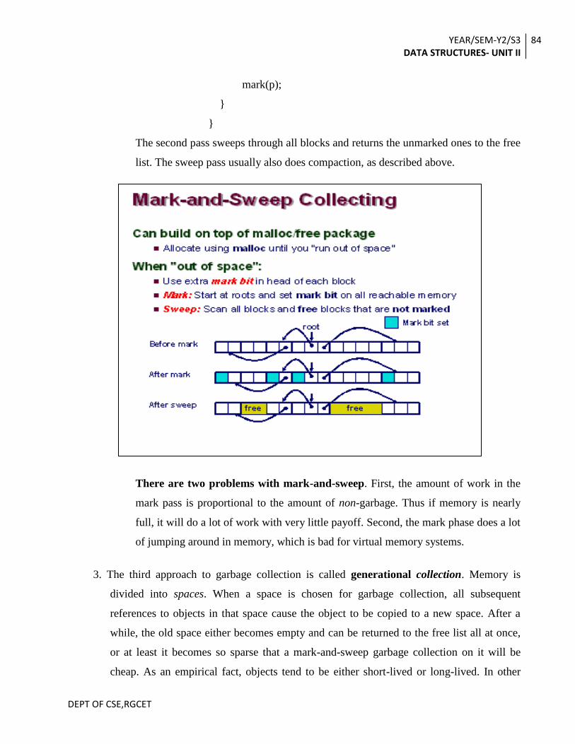
YEAR/SEM-Y2/S3 DATA STRUCTURES- UNIT II
84
DEPT OF CSE,RGCET
mark(p);
}
}
The second pass sweeps through all blocks and returns the unmarked ones to the free
list. The sweep pass usually also does compaction, as described above.
There are two problems with mark-and-sweep. First, the amount of work in the
mark pass is proportional to the amount of non-garbage. Thus if memory is nearly
full, it will do a lot of work with very little payoff. Second, the mark phase does a lot
of jumping around in memory, which is bad for virtual memory systems.
3. The third approach to garbage collection is called generational collection. Memory is
divided into spaces. When a space is chosen for garbage collection, all subsequent
references to objects in that space cause the object to be copied to a new space. After a
while, the old space either becomes empty and can be returned to the free list all at once,
or at least it becomes so sparse that a mark-and-sweep garbage collection on it will be
cheap. As an empirical fact, objects tend to be either short-lived or long-lived. In other

YEAR/SEM-Y2/S3 DATA STRUCTURES- UNIT II
85
DEPT OF CSE,RGCET
words, an object that has survived for a while is likely to live a lot longer. By carefully
choosing where to move objects when they are referenced, we can arrange to have some
spaces filled only with long-lived objects, which are very unlikely to become garbage.
COMPACTION :-
INSUFFICIENT MEMORY
Any of these methods can fail because all the memory is allocated, or because there is too
much fragmentation. A memory manager allocating real physical memory doesn't have that luxury.
The allocation attempt simply fails. There are two ways of delaying this catastrophe, compaction
and garbage collection.
COMPACTION
Compaction attacks the problem of fragmentation by moving all the allocated blocks
to one end of memory, thus combining all the holes.
Aside from the obvious cost of all that copying, there is an important limitation to
compaction: Any pointers to a block need to be updated when the block is moved.
Unless it is possible to find all such pointers, compaction is not possible.
Pointers can be stored in the allocated blocks themselves as well as other places in
the client of the memory manager. In some situations, pointers can point not only to
the start of blocks but also into their bodies.
For example, if a block contains executable code, a branch instruction might be a
pointer to another location in the same block.
Compaction is performed in three phases. First, the new location of each block is
calculated to determine the distance the block will be moved. Then each pointer is
updated by adding to it the amount that the block it is pointing (in)to will be moved.
Finally, the data is actually moved. There are various clever tricks possible to
combine these operations.
AUTOMATIC LIST MANAGEMENT

YEAR/SEM-Y2/S3 DATA STRUCTURES- UNIT II
86
DEPT OF CSE,RGCET
There are two principle methods used in automatic list management: the reference count
method and the garbage collection method.
Reference Count Method:
Each node has an additional count field that keeps a count (called the reference count)
of the number of pointers (both internal and external) to that node.
Each time that the value of some pointer is set to point to a node, the reference count in
that node is increased by1; each time the value of some pointer that had been pointing
to a node is changed, the reference count in that node is decreased by 1.
When the reference count in any node becomes 0, that node can be returned to the
available list of free nodes.
Each list operation of a system using the reference count method must make provision for
updating the reference count of each node that it accesses and for freeing any node whose
count becomes 0.
Figure illustrates the creation of the list using the reference count method. Each part of
that figure shows the list after an additional group of the foregoing statements has
been executed.
The reference count is shown as the leftmost field of each list node. Each node in that
figure is numbered according to the numbering of the nodes.
One drawback of the reference count method is illustrated by the foregoing example.
The amount of work that must be performed by the system each time that list
manipulation statement is executed can be considerable.
Whenever a pointer value is changed, all nodes previously accessible from that
pointer can potentially be freed.
Often , the work involved in identifying the nodes to be freed is not worth the
reclaimed space, since there may be ample space for the program to run to
completion without reusing any nodes.
YEAR/SEM-Y2/S3 DATA STRUCTURES- UNIT II
87
DEPT OF CSE,RGCET
After the program has terminated, a single pass reclaims all of its storage without having to
worry about reference count values.
One solution to this problem can be illustrated by a different approach to the previous example.
When the statement List9=null Is executed, the reference count in node 1 is reduced to 0 and node 1
is freed — that is, it is placed on the available list.
However, the fields of this node retain their original values, so that it still points
to nodes 2 and 11.
The reference count values in these two nodes remain unchanged. When
additional space s needed and node 1 is reallocated for some other use, the
reference counts in nodes 2 and 11 are reduced to 0 and they are then placed on
the available list.
This removes much of the word from the deallocation process and adds it to the
allocation process. If node 1 is never reused because enough space is available,
nodes 2, 11, 3, 4, 7 and 12 are freed during program execution.
For this scheme to word best, however, the available list should be kept as a
queue rather than as a stack, so that freed nodes are never allocated before nodes
that have not been used for the first time.
There are two additional disadvantages to the reference count method.
1. The first is the additional space required in each node for the count.
This is not usually an overriding consideration, however. The problem can be
somewhat alleviated if each list is required only a header node could be
referenced by more than one pointer.
The counts are kept in the first field of the header node. When the count in a
header node reaches 0, all the nodes on its freed and the counts in header
nodes pointed to be lstinfo fields in the list nodes are reduced.
If counts are to be retained in header nodes only, certain operations may have
to be modified.
One method of modification is to use the copy method in implementing these
operations.

YEAR/SEM-Y2/S3 DATA STRUCTURES- UNIT II
88
DEPT OF CSE,RGCET
Another method is to differentiate somehow between external pointers, which
represent lists, and “temporary” external pointers, which are used for
traversal.
When the count in a header node becomes 0, references to its list nodes
through temporary pointers become illegal.
2. The other disadvantage of the reference count method is that the count in the first
node of a recursive or circular list will never be reduced to 0.
Of course, whenever a pointer within a list is set to point to a node on that list,
the reference count can be maintained rather than increased, but detecting
when this is so is often a difficult task.
Garbage collection:
Under the reference count method, nodes are reclaimed when they become available
for reuse. The other principal method of detection and reclaiming free nodes us
caked garbage collection.
Under this method, nodes no longer in use remain allocated and undetected until all
available storage has been allocated.
A subsequent request for allocation cannot be satisfied until nodes that bad been
allocated, but are no longer in use are recovered.
When a request is made for additional nodes and there are none available, a system
routine called the garbage collector is called.
This routine searches through all of the nodes in the system, identifies those that are
no longer accessible from an external pointer, and restores the inaccessible nodes to
the available pool.
The request for additional nodes is then fulfilled with some of the reclaimed nodes
and the system continues processing user requests for more space. When available
spaces are used up again, the garbage collector is called once more.
Garbage collection is usually done in two phases.

YEAR/SEM-Y2/S3 DATA STRUCTURES- UNIT II
89
DEPT OF CSE,RGCET
The first phase, called marking phase, involves marking all nodes that are
accessible from an external pointer.
The second phase, called the collection phase, involves proceeding
sequentially through memory and freeing all nodes that have not been marked.
One field must be set aside in each node to indicate whether a node has or has not been
marked.
The marking phase sets the mark field to true in each accessible node. As the
collection phase proceeds, the mark field in each accessible node is reset to false.
Thus, at the start and end of garbage collection, all mark fields are false.
One aspect of garbage collection is that it must run when there is very little space
available.
This means that auxiliary tables and stacks needed by the garbage collector must be
kept to minimum since there is little space available for them.
An alternative is to reserve a specific percentage of memory for the exclusive use of
the garbage collector.
However, this effectively reduces the amount of memory available to the user and
means that the garbage collector will be called more frequently.
Whenever the garbage collector is called, all user processing comes to a halt while the
algorithm examines all allocated nodes in memory.
For this reason it is desirable that the garbage collector be called as infrequently as possible.
For real-time applications, in which a computer must respond to a user request within a
specific short time span, garbage collection has generally been considered an unsatisfactory
method of storage management.
Another important consideration is that users must be careful to ensure that ll lists are well
formed and that all pointers are correct.
Usually, the operations of a list processing system are carefully implemented so that
if garbage collection does occur in the middle of one of them, the entire system still
works correctly.
Thrashing:
It is possible that, at the time the garbage collection program is called, users are
actually using almost all the nodes that are allocated.

YEAR/SEM-Y2/S3 DATA STRUCTURES- UNIT II
90
DEPT OF CSE,RGCET
Thus almost all nodes are accessible and the garbage collector recovers very little
additional space.
After the system runs for a short time, it will again be out of space; the garbage
collector will again be called only to recover very few additional nodes, and the
vicious cycle starts again.
This phenomenon, in which system storage management routines such as garbage
collection are executing almost all the time, is called thrashing.
Clearly, thrashing is a situation to be avoided. One drastic solution is to impose the
following condition.
If the garbage collector is run and does not recover a specific percentage of the total
space, the user who requested the extra space is terminated and removed from the
system.
All of that user’s space is then recovered and made available to other users.
SCHORR-WAITE ALGORITHM:
Figure illustrates how this stacking mechanism works. Figure shows a list
before the marking algorithm begins.
The pointer p points to the node currently being processed, top points to the
stack top, and q is an auxiliary pointer.
The mark field is shown as the first field in each node. Figure b shows the same
list immediately after node 4 has been marked.
The path taken to node 4 is through the next fields of nodes 1,2, and 3. This
path can be retraced in reverse order, beginning at top and following along the
next fields.
Figure shows the list after node 7 has been marked. The path to node 7 from
the beginning of the list was from node 1.
Through node[1].next to node2, through node[2].lstinfo to node 5, through
node[5].next to node 6, and then from node[6].next to node 7.
The same fields that link together the stack are used to restore the list to its
original form. Note that the utype field in node 2 is stk rather than lst to
indicate that its lstinfo field, not its next field, is being used as a a=stack pointer.

YEAR/SEM-Y2/S3 DATA STRUCTURES- UNIT II
91
DEPT OF CSE,RGCET
The algorithm they incorporates these ideas is known as the Schorr-Waite
algorithm, after its discoverers.
Collection and Compaction
Once the memory locations of a given system have been marked appropriately, the
collection phase may begin.
The purpose of this phase is to return to available memory all those location that
were previously garbage (not used by any program but unavailable to any user). It is
easy to pass through memory sequentially examine each node in turn, and return
unmarked nodes to available storage.
For example, given the type definitions and declarations presented above, the following
algorithm could be used to return the unmarked nodes to an available list headed by avail:
for (p = 0; p <NUMNODES; p++) {
if (node[p]. mark! true) {
node[p]. next = avail;
avail = p;
} /* end if */
node[p].mark = FALSE;
} /*end for */
After this algorithm has completed, all unused nodes are on the available list, and all nodes
that are in use by programs have their mark fields turned off.
Though all nodes that are not in use are on the available list, the memory of the system may
not be in an optimal state for future use. This is because the interleaving of the occupied
nodes with available nodes may make much of the memory on the available list unusable.
For example, memory is often required in blocks (groups of contiguous nodes) rather than
as single discrete nodes one at a time.
The memory request by a compiler for space in which to store an array, would require the
allocation of such a block.
YEAR/SEM-Y2/S3 DATA STRUCTURES- UNIT II
92
DEPT OF CSE,RGCET
If, for example, all the odd locations in memory were occupied and all the even locations
were on the available list, a request for even an array of size 2 could not be honored, despite
the fact that half of memory is on the available list.
Although this example is probably not very realistic, could not be honored, despite the fact
that sufficient memory does indeed exist.
There are several approaches to this problem. Some methods allocate and free portions of
memory in blocks (groups of contiguous nodes) rather than in units of individual nodes.
This guarantees that when a block of storage is freed (returned to the available pool), a block
will be available for subsequent allocation requests.
Compaction
However, even if store is maintained as units of individual nodes rather than as blocks, it is
still possible to provide the user with blocks of contiguous storage.
The process of moving all used (marked) nodes to one end of memory and all the
available memory to the other end is called compaction, and an algorithm that
performs such a process is called a compaction (or compacting) algorithm.
The basic problem in developing an algorithm that moves portions of memory from one
location to another is to preserve the integrity of pointer values to the nodes being moved.
For example, if node(p) in memory contains a pointer q, when node(p) and node(q)
are moved, not only must the addresses of node(p) and node(q) be modified but the
contents of node(p) (which contained the pointer q) must be modified to point to the
new address of node(q).
In addition to being able to change addresses of nodes, we must have a method of
determining whether the contents of any node contain a pointer to some node( in
which case its value may have to be changed) or whether it contains some other data
type( so that no change is necessary).
The compaction algorithm is executed after the marking phase and traverses memory
sequentially. Each marked node, as it is encountered in the sequential traversal, is

YEAR/SEM-Y2/S3 DATA STRUCTURES- UNIT II
93
DEPT OF CSE,RGCET
assigned to the next available memory location starting from the beginning of
available memory.
When examining a marked node nd1 that points to a node nd2, the pointer in
nd1 that now points to nd2 must be updated to the new location where nd2
will be moved.
That location may not yet be known because nd2 might be at a later address
than nd1.
nd1 is therefore placed on a list emanating from nd2 of all nodes that
contain pointers to nd2, so that when the new location of nd2 is determined,
nd1 can be accessed and the pointer to nd2 contained in it modified.
Now consider a single sequential pass of the algorithm. If a node nd1 points to a
node nd2 that appears later in memory, by the time the algorithm reaches nd2
sequentially, nd1 will have already been placed on the adjustment list of nd2.
When the algorithm reaches nd2, therefore, the pointers in nd1 can be
modified.
But if nd2 appears earlier in memory, when nd2 is reached, it is not yet
known that nd1 points to it; therefore the pointer in nd1 cannot be adjusted.
For this reason the algorithm requires two sequential passes. The first places
nodes on adjustment lists and modifies pointers in nodes that it finds on
adjustment lists.
The second clears away adjustment lists remaining from the first pass and
actually moves the nodes to their new locations. The first pass may be
outlined as follows:
1. Update the memory location to be assigned to the next marked node, nd.
2. Traverse the list of nodes pointed to by header(nd) and change the appropriate
pointer fields to point to the new location of nd.
3. If the utype field of nd is lst and lstinfo(nd) is not null, place nd on the list of the
nodes headed by header (lstinfo(nd)).
4. If next(nd) is not null, place nd on the list of the nodes headed by header(next)(nd).

YEAR/SEM-Y2/S3 DATA STRUCTURES- UNIT II
94
DEPT OF CSE,RGCET
Once this process has been completed for each marked node, a second pass through memory
will perform the actual compaction. During the second pass we perform the following
operations:
1. Update the memory location to be assigned to the next marked node,nd.
2. Traverse the list of nodes pointed to be header(nd) and change the appropriate
pointer fields to point to the new location of nd.
3. Move nd to its new location.
Variations of garbage collection:
Applications that are executing in real time(for example, computing the trajectory of
a spaceship, or monitoring a chemical reaction) cannot be halted while the system is
performing garbage collection.
In these circumstances it is usually necessary to dedicate a separate processor
devoted exclusively to the job of garbage collection.
When the system signals that garbage collection must be performed, the
separate processor begins executing concurrently with the applications
program.
Because of this simultaneous execution, it is necessary to guarantee that
nodes that are in the process of being acquired for use by an application
program are not mistakenly returned to the available pool by the collector.
Another subject of interest deals with minimizing the cost of reclaiming(getting back)
unused space.
In the methods mentioned above, the cost of reclaiming any portion of storage is has
been directed toward designing a system in which the cost of reclaiming a portion of
storage is proportional to its lifetime.
Thus, by reducing the cost of retrieving portions of memory required for short time
periods at the expense of the cost of retrieving portions of memory with longer
lifespans, the overall cost of the garbage collection process will be reduced.

YEAR/SEM-Y2/S3 DATA STRUCTURES- UNIT II
95
DEPT OF CSE,RGCET
The process of garbage collection is also applied to reclaiming unused space in secondary
devices(for example, a disk).
Although the concept of allocation and freeing space is the same(that is, space may
be requested or released by a program), algorithms that manage space on such
devices often cannot be translated efficiently from their counterparts that manipulate
main memory.
The reason for this is that the cost of accessing any location in main memory is the
same as that of accessing any other location in main memory.
In secondary storage, on the other hand, the cost depends on the location o storage
that is currently being accessed as well as the location we desire to access.
It is very efficient to access a portion of secondary storage that is in the same block
that is now being accessed; to access a location in a different block may involve
expensive disk seeds.
For this reason, device management systems for offline storage try to minimize the
number of such accesses.