Stack Sampling Technical Information: A Collection of ... · between the fuel heat value and dry effluent that permits a constant (F Factor ... The method calculating emission rates

METHOD FOR CALCULATING

POWER PLANT EMISSION RATE

BY

R. T. Shigehara, R. M. Neulicht: and W. S. Smith**

Introduction

In the final State Implementation Plans submitted by all 50 States,

the District of Columbia, Puerto Rico, American Samoa, Guam, and the

Virgin Islands in response to the 1970 Clean Air Act, most of the regu-

lations for the control of particulate, sulfur dioxide, and nitrogen

oxide emissions from fuel burning sources are expressed in pounds of

emissions per million Btu of heat input (lb/lo6 Btu)'. The Federal New

Source Performance Standards* regulating the same pollutants from fossil

fuel-fired steam generating units of more than 250 million Btu/hr heat

input are expressed in the same terms. To arrive at this expression, the

Federal perfromance standard regulations call for the determination of the

pollutant concentration (C), the effluent volumetric flow rate (Q,), and the

heat input rate (QH). In addition, the heat input rate must be confirmed by

a material balance over the steam generator system.

The purpose of this paper is to present an alternative method for arriv-

ing with improved accuracy at the expression of lb/lo6 Btu called for by the

State and Federal regulations without having to determine effluent gas volu-

metric flow rate, fuel rate, or fuel heat content.

Published in Stack Sampling News l(1): 5-9, July 1973

* Emission Measurement Branch, ESED, OAQPS, EPA ** Entropy Environmentalists, Inc.

1

Derivation of the F-Factor Method

Standard Method

In the standard method of calculating emission rates:

c Qs E = - QH

(1)

where: E = pollutant emission, lb/lo6 Btu.

C = pollutant concentration, dry basis, lb/scfd.

Q, = dry effl uent volumetric flow rate, scfdjhr.

Q, = heat input rate, lo6 Btu/hr.

F-Factor Method

When the laws of conservation of mass and energy are applied, the

following must hold true:

(2)

where: V, = theoretical dry combustion products per pound of fuel burned,

scfd/lb.

HHV = high heating value, lo6 Btu/lb.

20.9 - %O _ 2 - excess air correction factor. 20.9

Solving Equation 2 for the ratio Q,/Q, and substituting into Equation 1

yields: V 20.9

E = ' (i6V) (20.9 - "002~) (3)

The amount of dry effluent gas (Vs) generated by combustion of a fossil

fuel can easily be calculated from the ultimate analysis. The high heating

value can be obtained from standard calorific determinations. The ratio, F,

between Vs and HHV can be calculated for various fossil fuels; F is the efflu-

ent gas generated per lo4 Btu heat content:

vS F = ‘TmqTmj- (4)

Values for F calculated from data obtained from the literature are

summarized in Table I. Of course, this ratio can be calculated for each

specific case, but the dry effluent per lo4 Btu varies no more than about

5 3%. For this reason, these ratios will be considered as constants and

will hereafter be called "F Factors." The use of these F Factors, as will

be discussed later, eliminates the need for ultimate and calorific analyses.

A list of average F Factors derived from Table I is shown in Table II.

3

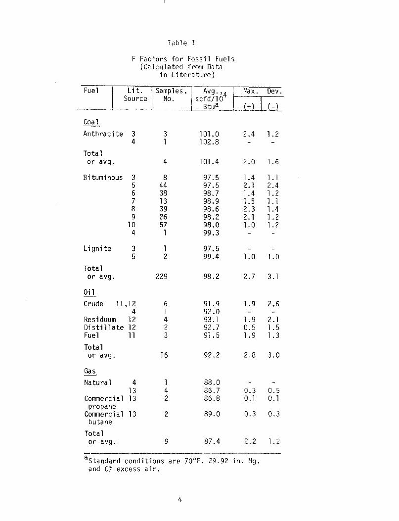
Table I

F Factors for Fossil Fuels (Calculated from Data

Coal

Anthracite 3 4

Total or avg.

Bituminous 3

z 7 8

1: 4

Lignite 3 5

Total or avg.

Oil

Crude 11,12 4

Residuum 12 Distillate 12 Fuel 11

Total or avg.

Gas

Natural 4 13

Commercial 13 propane

Commercial 13 butane

Total or avg.

in Literature)

3 101.0 2.4 1.2 1 102.8 - -

4 101.4 2.0 1.6

8 97.5 1.4 1.1 44 97.5 2.1 2.4 38 98.7 1.4 1.2 13 98.9 1.5 1.1 39 98.6 2.3 1.4 26 98.2 2.1 1.2 57 98.0 1.0 1.2

1 99.3 - -

1 97.5 - - 2 99.4 1.0 1.0

229 98.2 2.7 3.1

6 91.9 1.9 2.6 1 92.0 4 93.1 119 211 2 92.7 0.5 1.5 3 91.5 1.9 1.3

16 92.2 2.8 3.0

1 88.0 - - 4 86.7 0.3 0.5 2 86.8 0.1 0.1

2 89.0 0.3 0.3

9 87.4 2.2 1.2 _ --_----- --____-.-.

aStandard conditions are 7O"F, 29.92 in. Hg, and 0% excess air.

Table II. Average F Factorsa

Fuel -___. . _ -------__-- - ----- - .._

I -.__ .__.-_ ..__ __

F Fat ors scfd/lO Btub 4

.-- --.~.--. - -----

Coal-anthracite 101.4

Coal-bituminous, lignite 98.2

Oil-crude, residuum, distillate, fuel oil

1

92.2

Gas-natural, butane, propane 87.4 ------ -_- ------___

aDerived from Table I.

b700F, 29.92 in. Hg., and 0% excess air.

Use of F Factors

Emission Rate Calculation

When Q, and Q, are not measured or are unobtainable, F Factors can be used

to calculate E. Substituting Equation 4 into Equation 3 we obtain:

E = C F (20ag 2090

- %02)

where: F = F Factor from Table II, in scfd/104 Btu.

Equation 5 shows that E can be obtained by simply measuring the pollutant

concentration and percentage oxygen and by knowing the type of fuel being burned.

Q, and Q, are no longer required.

Material Balance Check

If Q, and Q, are measured, F Factors can be used to check sampling data by

comparing them with Fm.

where: QS Fm = Q H

5

Fuel AI'I~ !ysis ChecL

If ultimate and proximate analyses are made, F Factors can be used

to check the accuracy of such analyses by comparing them with Vs/HHV which

is the calculated amount of dry effluent gas generated per lo4 Btu heat

content.

Discussion

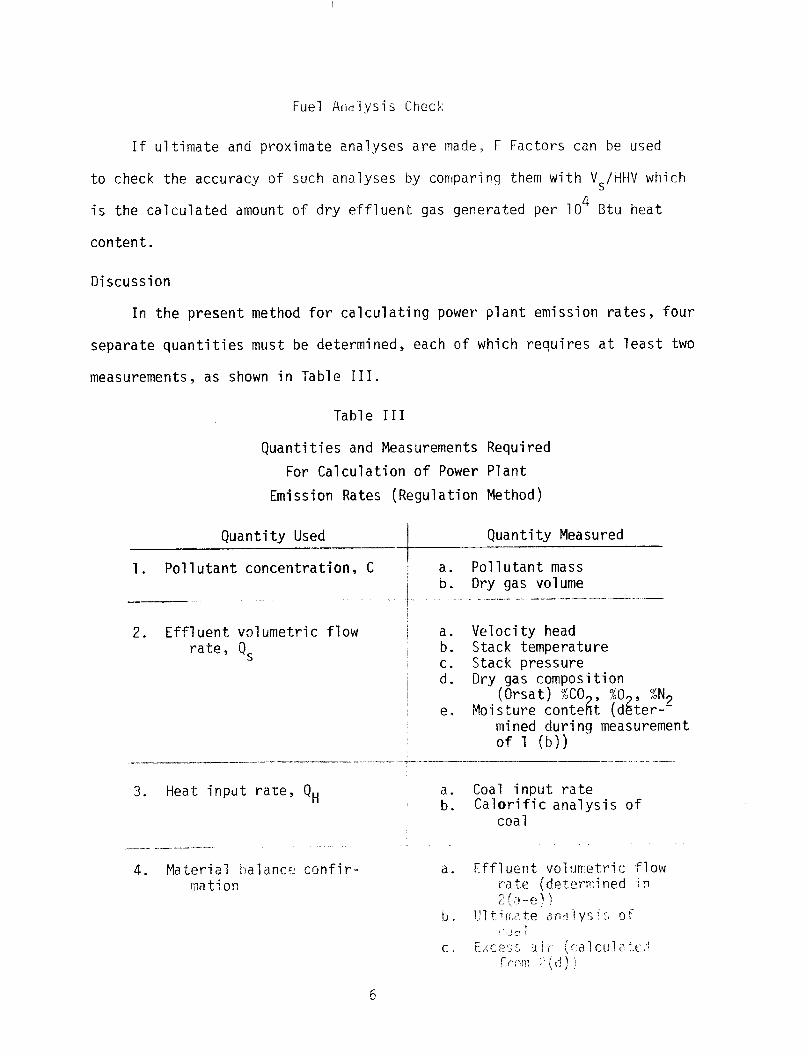
In the present method for calculating power plant emission rates, four

separate quantities must be determined, each of which requires at least two

measurements, as shown in Table III.

Table III

Quantities and Measurements Required

For Calculation of Power Plant

Emission Rates (Regulation Method)

Quantity Used Quantity Measured

1. Pollutant concentration, C ; a. Pollutant mass i b. Dry gas volume j - . - ---.- . - I

2. Effluent volumetric flow I / a. Velocity head rate, Qs b. Stack temperature

:: Stack pressure Dry gas composition

! (Orsat) %CO %O %N e. Moisture conteit (dgier-'

mined during measurement of 1 (b))

.l-l_l-- __._.- ----______- __.-_______ ----__I___ ._-..._.... -.. --.

3. Heat inptit rate, QH

.--- _.__ -- ..---.

4. Material !lalancc confir mation

a. Coal input rate b. Calorific analysis of

coal

From Table III, it is obvious that .the use of F Factors in calculating

E requires fewer measurements than are required by methodology in current

use. Because there are fewer measurements, the inaccuracies attendant to

measuring items 2 through 4 (except for 2d) are not included in the final

results. Granted that those measurements in 2 must be made for isokinetic

sampling, but the errors made do not contribute directly to the emission stan-

dard calculation.

Conclusion

It has been shown that, for a given type of fuel, a relationship exists

between the fuel heat value and dry effluent that permits a constant (F Factor)

to be calculated within + 3% deviation.

This implies that: (1) pollutant emissions in lb/106.Btu can be easily

calculated when only pollutant concentration, 02 concentration, and fuel type

are known, thus eliminating the need for measuring effluent volumetric flow rate

and heat input rate; (2) the inconsistencies that arise in measuring the heat

input rate are eliminated whi7e at most a maximum error of 3% may be propagated

from the F Factor to the pollutant emission rate; and (3) if effluent volumetric

flow rate (Q,) and heat input rate (Q,) are measured, an Fm Factor can be cal-

culated from those values and compared with the F Factor as a mass balance check.

In short, use of the F Factor provides a method less complex than the one

now employed for calculating power plant emission rates and evaluating the

sampling data.

7

1.

2. Federal Register, Standards of Performance for New Stationary Sources,

36:247, Part II (Dec. 23, 1971).

3. Perry, John H., ed., Chemical Engineers' Handbook, 4th ed., p. 9-3,

McGraw-Hill Book Company, N. Y. (1963).

4. North American Combustion Handbook, North American Manufacturing Co., 13,

Cleveland (1965).

5. Hodgman, Charles D., Handbook of Chemistry and Physics, 43rd ed., 1943 - -

1944, Chemical Rubber Publishing Co., Cleveland (1961).

6. Analyses of Tipple and Delivered Samples of Coal, U. S. Dept. of Interior, - --

U.S. Bureau of Mines, Washington, D. C., Publication No. USBMRI 7588 (1972

7.

8.

9.

10.

References

Duncan, L. J., Analysis of _Final State Imp!-enentatisn !.!_a~ -

Rules and Regulations Environmental Protection Agency, Research .___ - --

Triangle Park, North Carolina 27711, Publication No. APTD-1334 (1972).

U.S. Dept. of interior, U.S. Bureau of Mines, Washington, D. C., Publica-

tion No. USBMRI 7490 (1971).

U.S. Dept. of Interior, U.S. Bureau of Mines, Washington, D. C., Publica-

tion No. USMBRI No. 7346 (1970).

U.S. Dept. of Interior, U.S. Bureau of Mines, Washington, 0. C., Publica-

tion No. !JSMBRI 7219 (1969).

U.S. Dept. of Interior, U.S. f'illreau of Mines, Washington, D. C., Publica-

tion No. USMBRI 6792 (1956).

1.

8

References {Continued)

11. Hodgman, Carles D., ed. Handbook of Chemistry and Physics, 43rd ed.,

1936, Chemical Rubber Publishing Co., Cleveland (1961).

12. North American Combustion Handbook, North American Manufacturing Co., 31, ~-

Cleveland (1965).

.

EMISSION C;lRRE",TION FACTOR for FQSSii FUEL-FIRED STEAM GENERATORS

CO2 CONCENTRATION APPRQACh

Roy Neulicht*

Introduction

The Federal Standards of Performance for New Stationary Sources

regulating particulate matter, sulfur dioxide, and nitrogen oxide

emissions from fossil fuel-fired steam generating units of more than 63

million kcal/hr (250 million Btu/hr) heat input are expressed in terms

of mass per unit of heat input, g/lo6 cal (lb/lo6 Btu). To arrive at

this emission rate, the existing method' requires determination of the

pollutant concentration (C), the effluent volumetric flow rate (Q,), and

the heat input rate (Qh). An F-Factor approach requiring determination

of the fuel type, pollutant concentration (C), and the oxygen concentra-

tion (%02) has been proposed2 as the reference method to replace the

existing method.

The purpose of this paper is to present a third method, based on the

F-Factor approach and employing a dilution correction factor based on

measuring the carbon dioxide rather than oxygen concentration. This method,

which will be called the Fc-Factor method,is based on two facts:

1. The comparison of the theoretical carbon dioxide produced during

combustion to the measured carbon dioxide provides an exact basis

for dilution correction.

2. Within any fossil fuel type category, the ratio of the volume of

carbon dioxide to the calories released is essentially a constant.

The method has two advantages:

1. Emission rates may be determined from wet basis concentration

measurements without recalculation of the Fc-Factor. -_- * Emission Measurement Branch, ESED, OAQPS, EPA, RTP, NC Published in Stack Sampling News 2(8): 6-11 I Febr!lary 1975

2. Use of CO2 for correcting for dilution provides flexibility

A by providing an additional method for determining emission

rates; for example, in some cases measuring CO2 may be more

convenient than measuring 02.

One disadvantage of the CO2 correction factor is that it cannot be used

after control devices that alter the CO2 concentration (e.g., wet scrub-

bers that remove CO2) or in situations where CO2 is added.

Derivation of Fc-Factor Method

The method calculating emission rates as promulgated in the Federal

Register' is:

Q E=C> QH

(‘1

where: E = pollutant emission, g/lo6 cal (lb/106Btu)

C = pollutant concentration, dry basis, g/dscm, (lb/dscf)

Q,= dry effl uent volumetric flow rate, dscm/hr (dscf/hr)

Q,= heat input rate, lo6 cal/hr (lo6 Btu/hr)

When the laws of conservation of mass and energy are applied, the following

must hold true:

(2)

where: Vt= total theoretical dry combustion products per unit

mass of fuel burned, dscm/g (dscf/lb)

HHV= high heating value, lo6 Cal/g (lo6 Btu/lb)

11

%co*m -- = dilution correction factor, ratio of measured car- %C02 t

bon dioxide and theoretical carbon dioxide produced

from combustion, dry basis

Solving Equation 2 for the ratio Q,/QH and substituting into

Equation 1 yields:

V Substituting $- (100) for %COzt yields:

t

E=C v ’

i ) + (100) t

(3)

(4)

where: Vc= theoretical volume of carbon dioxide-produced per unit

mass of fuel burned, scm/g (scf/lb)

Elimination of Vt from Equation 4 and rearrangement yields:

E = c c 1001 PC' %COzm/ ;HHV 1

or

E=cj$C02mj c "100 ' (F )

(5)

(6)

where: vC

Fc= HHV ~ , the ratio of theoretical CO2 generated by

combustion to the high heating valve of the fuel com-

busted, scm/106 cal (scf/lO' Btu).

The high heating value of the fuel combusted can be obtained from

12

standard calorific determinations. The amount of theoretical carbon

dioxide generated by combustion can eas ily be calculated from the ult

calculated for various fossil mate analysis. The ratio, Fc, has been .

i-

fuels from data obtained from the literature; these calculated ratios

are summarized in Table I. For any fuel type, the ratio is found to

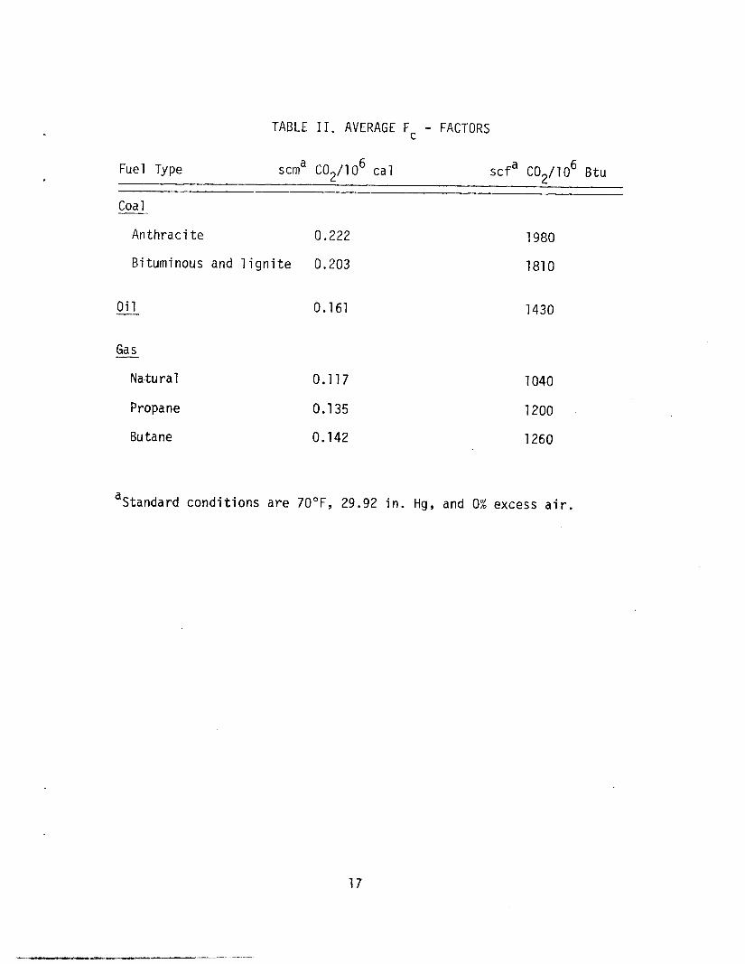
be a constant with a maximum deviation of It_ 5.9%. Average Fc - Factors

for each fuel type are given in Table II.

Note that Equation 6 for the determination of the pollutant emission

rate (E) has been developed in terms of dry measurements. However, it

is a simple matter to show that wet basis measurements may be used. Given

Equation 6 and multiplying both the measured pollutant concentration (C)

and the measured carbon dioxide concentration (%COpm) by the dry mole frac-

tion (D) of the effluent gas yields;

E = [(C)(WI (7)

or

03)

where: Cw= pollutant concentration, wet basis, g/scm (lb/scf)

%COzw= measured concentration of carbon dioxide, wet basis,

(expressed as percent).

Equations 6 and 8 show that, using the average Fc - Factor approach,

the pollutant emission rate (E) can be obtained by simply knowing the type

of fuel burned and measuring the pollutant and carbon dioxide concentrations

13

on either a wet or dry basis.

Determination of Fc - Factor -

Rather than use an average Fc - Factor, the Fc - Factor can be de-

termined on an individual case-by-case basis. As already stated, the

high heating value of the fuel is determined from standard calorific

determinations. The theoretical carbon dioxide generated by combustion

is easily calculated from the following equations based on stoichiometry3

and on information from an ultimate fuel analysis:

or

vc= 0.200 x 1

Vc= 0.321 %C

o-4 SC scm CO2

0 g fuel

scf co2

lb fuel

where: %C= percent carbon by weight determined from

ultimate analysis.

Given the definition of the Fc - Factor,

Fc= 4

and substituting Equations 9 and 10 yields:

F = 0.200 x 1o-4 %C C HHV for me

k ric units of

scm/lO cal

(9

(10)

(11)

02)

and

F = 0.321 %C C HHV- for En

8 lish units of

scf/lO Btu (13)

Note: %C and HHV must be on a consistent basis, e.g., if %C is deter-

mined on an as-received basis, HHV must also be on an as-received basis.

14

Conclusion

It has been shown that, for a given fuel type, a relationship

exists between the fuel calorific value and the theoretical effluent

carbon dioxide, which permits an average Fc - Factor to be calculated

within f 5.9% deviation. - This provides a method for calculating power

plant emission rates that may be used when the pollutant concentration,

carbon dioxide concentration, and fuel type are known. The equation

for such a calculation is given as follows:

(14)

where: E = pollutant emission, g/lo6 cal (lb/lo6 Btu)

C = pollutant concentration, g/scm (lb/scf)

%C02 = carbon dioxide content by volume (expressed as

percent)

Fc = a factor representing a ratio of the volume of

theoretical carbon dioxide generated to the

calorific value of the fuel combusted.

Note: C and %C02 may be measured either on a wet or

dry basis provided that the same basis is used

for each.

Furthermore, average values of Fc are given for each fossil fuel

type, and the necessary equations for determining the Fc - Factor on a

case-by-case basis are presented.

15

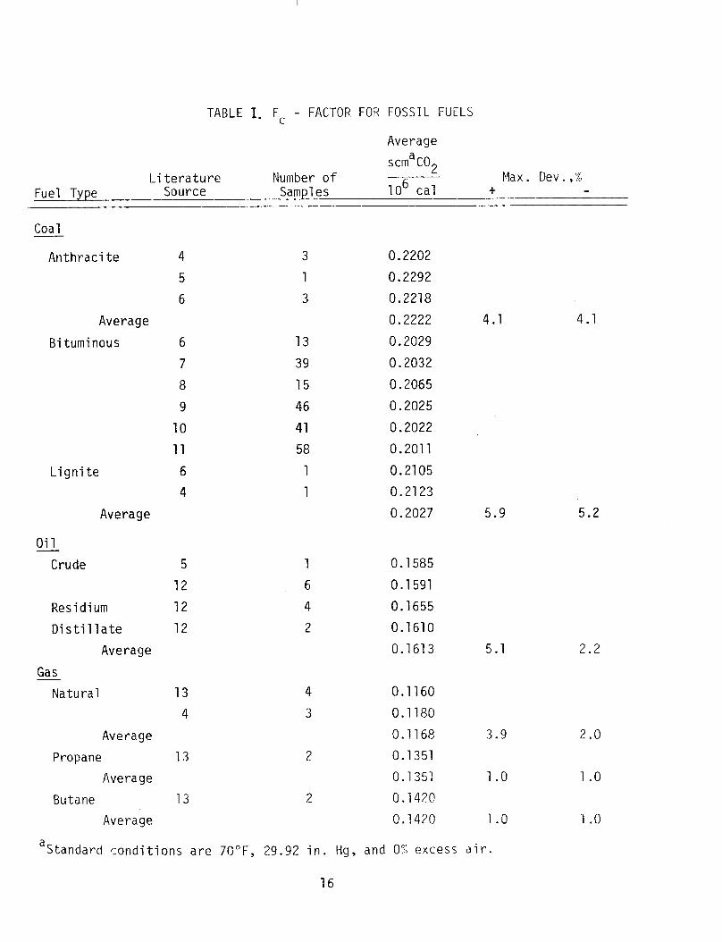
TABLE I. Fc - FACTOR FOR FOSSIL FUELS

Average

Fuel Type Literature

Source

scmaco2 Number of --__I

Samples 106 cal Max. Dev.,%

+ -

Coal

Anthracite

Average

Bituminous

Lignite

Average

Oil

Crude

Residium

Distillate

Average

Gas

Natural

Average

Propane

Average

Butane

Average

6 13

7 39

8 15

9 46

10 41

11 58

6 1

4 1

5 1 0.1585

12 6 0.1591

0.2202

0.2292

0.2218

0.2222 4.1 4.1

0.2029

0.2032

0.2065

0.2025

0.2022

0.2011

0.2105

0.2123

0.2027 5.9 5.2

655

610

613 5.1 2.2

160

4 3 0.1180

0.1168 3.9 2.0

13 2 0.1351

0.135? 1.0 1.0

13 2 0.1420

0.1420 I .o 1 .o

aStandard conditions are 70"F, 29.92 in. Hg, and 0% excess air.

16

.

TABLE II. AVERAGE Fc - FACTORS

Fuel Type suna CO2/10 6 cal scfa C02/106 Btu

Coal --

Anthracite 0.222 1980

Bituminous and lignite 0.203 7810

Oil

Gas

0.161 1430

Natural 0.117 1040

Propane 0.135 1200

Butane 0.142 1260

'Standard conditions are 7O"F, 29.92 in. Hg, and 0% excess air.

17

REFERENCES

1. Federal Register, Standards of Performance for New Stationary

Sources, 36:247, Part II, December 23, 1971. -

2. Federal Register, Proposed Emission Monitoring and Performance -

Testing Requirements for New Stationary Sources, 39:177, Part II, -

September 11, 1974.

3. North American Combustion Handbook, North America Manufacturing

co., Cleveland, 1965, p.48.

4. Perry, John H. fed.), Chemical Engineers' Handbook, 4th ed.,

McGraw Hill Book Company, N.Y., 1963, p.9-3.



6. Steam, The Babcox and Wilcox Co., New York, 1963, p.2-10.

7. Analysis of Tipple and Delivered Samples of Coal, U.S. Dept. of

Int., U.S. Bureau of Mines, Washington, D.C., Publication No. USBMRI 7588,

1972.

8. U.S. Dept. of Interior, U.S. Bureau of Mines, Washington, D.C.

Publication No. USBMRI 7490, 1971.



10. U.S. Dept. of Interior, U.S. Bureau of Mines, Washington,D.C.




18

REFERENCES(Continued)

. 12. North American Combustion Handbook, North America Manufacturing ___ -.-.-- --


13. North American Combustion Handbook, North America Manufacturing --


14. Shigehara, R.T. et al. "A Method for Calculating Power Plant

Emission Rates," Stack Sampling News, Volume 1, Number 1, July, 1973.

‘I 9

DERIVATION OF EQUATIONS FOR CALCULATING POWER PLANT EMISSION RATES

02 Based Method - Wet and Dry Measurements

R. T. Shigehara & R. M. Neulicht*

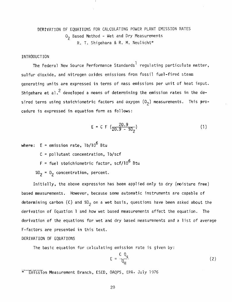
INTRODUCTION

The Federal New Source Performance Standards' regulating particulate matter,

sulfur dioxide, and nitrogen oxides emissions from fossil fuel-fired steam

generating units are expressed in terms of mass emissions per unit of heat input.

Shigehara et al.L developed a means of determining the emission rates in the de-

sired terms using stoichiometric factors and oxygen (02) measurements. This pro-

cedure is expressed in equation form as follows:

E = C F Czo ;“:gyo > . "2

where: E = emission rate, lb/lo6 Btu

C = pollutant concentration, lb/scf

F = fuel stoichiometric factor, scf/106 Btu

%02 = O2 concentration, percent.

Initially, the above expression has been applied only to dry (moisture free)

based measurements. However, because some automatic instruments are capable of

determining carbon (C) and %02 on a wet basis, questions have been asked about the

derivation of Equation 1 and how wet based measurements affect the equation. The

derivation of the equations for wet and dry based measurements and a list of average

F-factors are presented in this text.

DERIVATION OF EQUATIONS

The basic equation for calculating emission rate is given by:

c Qs EC-..-- QH

(2)

* Emission Measurement Branch, ESED, OAQPS, EPA, July 1976

(1)

20

.

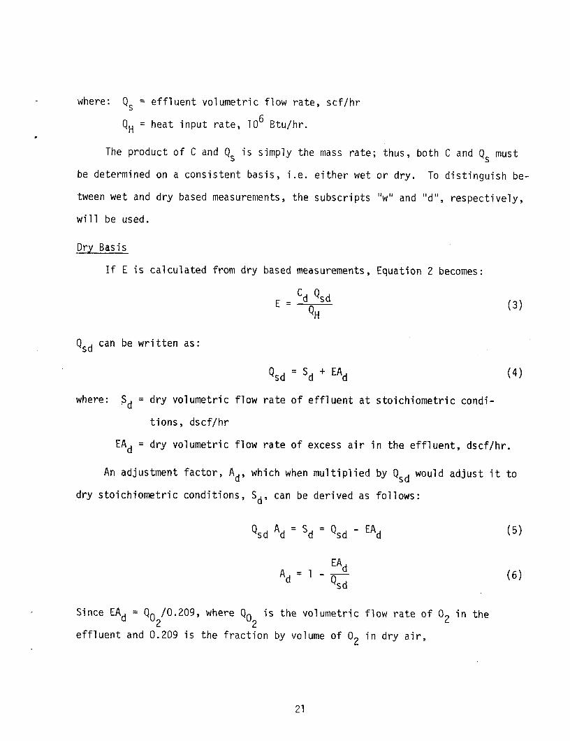
where: Qs = effluent volumetric flow rate, scf/hr

Q, = heat input rate, lo6 Btu/hr.

The product of C and Q, is simply the mass rate; thus, both C and Q, must

be determined on a consistent basis, i.e. either wet or dry. To distinguish be-

tween wet and dry based measurements, the subscripts "w" and "d", respectively,

will be used.

Dry Basis

If E is calculated from dry based measurements, Equation 2 becomes:

E= 'd Qsd

QH (3)

Q sd can be written as:

Q sd = Sd + EAd (4)

where: 'd

= dry volumetric flow rate of effluent at stoichiometric condi-

tions, dscf/hr

EAd = dry volumetric flow rate of excess air in the effluent, dscf/hr.

An adjustment factor, Ad, which when multiplied by Q,d would adjust it to

dry stoichiometric conditions, Sd$ can be derived as follows:

Q,, Ad = sd = Q,, - EAd (5)

EAd -- Ad = ' Qs, (6)

Since EAd = Q. /0.209, where Q, 2 2

is the volumetric flow rate of O2 in the

effluent and 0.209 is the fraction by volume of O2 in dry air,

21

Ad = 1 Q”*

- Tj-.209 Q,,

Noting that Q, /Q 2 sd

is the proportion by volume of O2 in the dry effluent mix-

ture (Ozpd) and substituting into Equation 7, Ad becomes:

0 Ad=l-&& .

20.9 - %OPd =

20.9

20.9 - %02d and sd = Q,, ( 20.9 1

Substituting Equation 9 into Equation 2 yields:

E 'd 20.9 = 'd Q, 20.9 - %02d

(8)

(9)

(10)

The ratio, S,/Q,, is simply the dry effluent gas at stoichiometric conditions

generated per unit of heat input and can be calculated from ultimate and calori-

fit analyses of the fuel. These calculated ratios are defined as Fd and are

surrunarized in Table I. Inserting Fd = S,/Q,,

Equation 10 can be rewritten in its final form as:

20.9 E = 'd Fd 20.9 - %Ozd

(11)

22

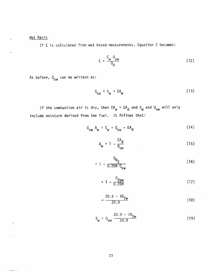
Wet Basis

If E is calculated from wet based measurements, Equation 2 becomes:

E cw Qsw = Q,

As before, Qs, can be written as:

Q SW = SW + EAw

If the combustion air is dry, then EA, = EAd and SW and Q,, will only

include moisture derived from the fuel. It follows that:

Q,, A, = SW = Q,, - EAd

EAd Aw=Lq SW

Q"* = l- 0.209 Q,,

= l- & .

= 20.9 - %02w

20.9

sw = Qsw 20.9 - %02w

20.9

(12)

(13)

(14)

(15)

(16)

(17)

(18)

(19)

23

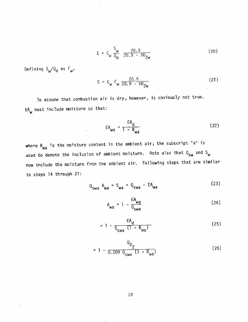
sw 20.9 E = cw 4, 20.9 - %o*w

Defining SW/Q, as Fw'

E = Cw Fw 2. ;";gso . a 2w

To assume that combustion air is dry, however, is obviously not true.

EA, must include moisture so that:

EAd EAwa = 1 - B

wa

(20)

(21)

(22)

where B,, is the moisture content in the ambient air; the subscript "a" is

used to denote the inclusion of ambient moisture. Note also that Q,, and SW

now include the moisture from the ambient air. Following steps that are similar

to steps 14 through 21:

Q swa Awa = Swa = Qswa - EAwa

EAwa A =l-4

wa swa

EAd = ‘-9 (1-B

swa wa)

QQ2 = l- 0.209 Qswa (1 - Bwa)

(23)

(24)

(25)

(26)

24

= 20.9 (1 - Bwa) - %02wa

20.9 (1 - Bwa)

s 20.9 (1 - Bwa) - %02wa

wa = Qswa 20.9 (1 - Bwa)

S wa E - = 'wa Q,

20.9 (1 - Bwa)

20.9 (1 - Bwa) - %02wa

Defining Swa/Q, as Fwa:

E 20.9 (1 - B,,)

= 'wa Fwa 20.9 (1 - Bwa) - %02wa

(27)

(28)

(29)

(30)

(31)

The inclusion of ambient air in Fwa, however, is undesirable in that it

becomes a variable. Written in terms of Fw, i.e. where ambient moisture is not

included, Fwa can be written as:

ThA (Bwa)

S F =wa=

sw + m

wa QH QH (32)

25

-.-

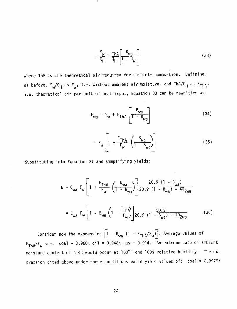
(33)

where ThA is the theoretical air required for complete combustion. Defining,

as before, SW/Q, as Fw, i.e. without ambient air moisture, and ThA/QH as FThA'

i.e. theoretical air per unit of heat input, Equation 33 can be rewritten as:

B F wa = Fw + FThA 1 1 1 -waBwa (34)

(35)

Substituting into Equation 31 and simplifying yields:

= 'wa Fw [1 - Bwa (1 - +$I]*O.9 (1 -':I, - %Ozwa (36)

Consider now the expression C

1 - Bwa (1 - FThA'Fw$ Average values of

FThA/Fw are: coal = 0.960; oil = 0.948; gas = 0.914. An extreme case of ambient

moisture content of 6.4% would occur at 100°F and 100% relative humidity. The ex-

pression cited above under these conditions would yield values of: coal = 0.9975;

oil = 0.9967; and gas -; G-9945. Therefore, neglecting this cited expression

would introduce ii positive bias of no more than 0.25 to 0.55%. Understanding

this, Equation 36 simplifies to its final form:*

20.9 --- E = 'wa Fw 20.9 (1 - Bwa) - %02wa (37)

Average values of Fw are listed in Table II. From Tables I and II it can

be seen that Fd fdCtorS have a maximum arithmetic deviation Of f 3.1 percent

and Fw factors, f 3.8 percent.

REFERENCES

1. Standards of Performance for New Stationary Sources. Federal Register.

(Washington) Part II. 363247, December 23, 1971.

2. Shigehara, R. T., R. M. Neulicht, and W. S. Smith. A Method for Calculating

Power Plant EmissiGn Rates, Stack Sampling News. I-:5-9, July 1973.

-

* This equation was originally derived by G. F. McGowan, Vice President, Environmental Technology Division, Lear Siegler, Eng7ewood, Colorado.

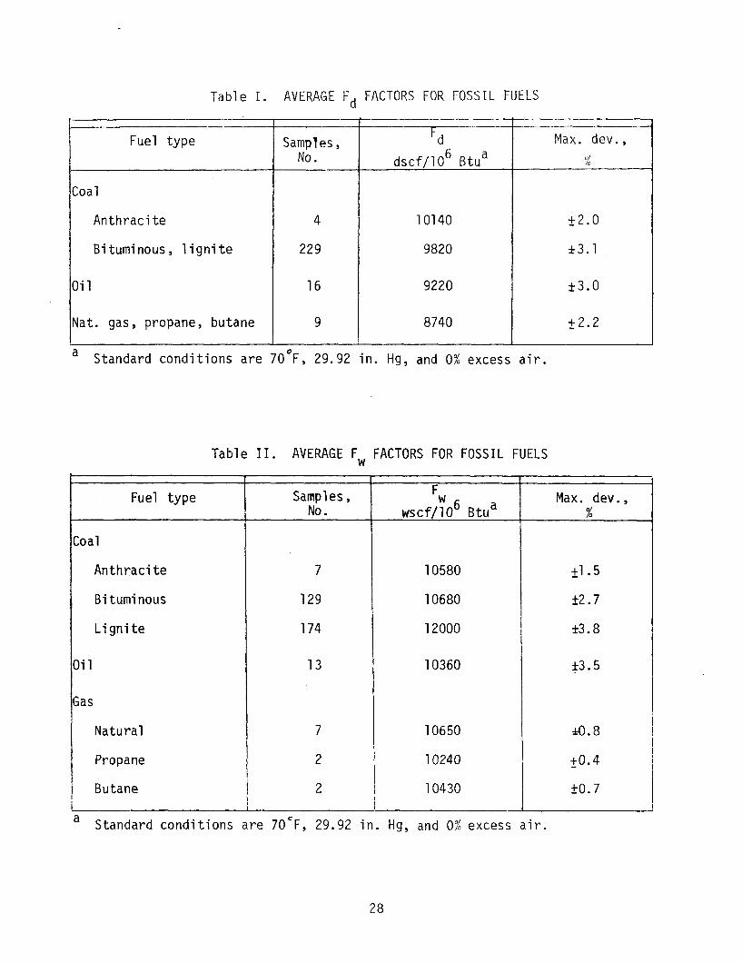
Table AVERAGE Fd FACTORS FOR FOSSIL FUELS

Fuel type

Coal

Anthracite

Bituminous, lignite

I Oil

Nat. gas, propane, butane 9

Samples, No.

4

229

16

- .~

'd - - . I - -

dscf/106 Btua

10140

9820

9220

8740

Max. dev.,

%

+2.0

zk3.1

f3.0

+2.2

a Standard conditions are 70°F, 29.92 in. Hg, and 0% excess air.

Table II. AVERAGE Fw FACTORS FOR FOSSIL FUELS

Samples, No.

Fuel type Fw wscf/106 Btua

10580

10680

12000

10360

Coal

Anthracite 7

Bituminous 129

Lignite 174

Oil 13

Gas

Natural

Propane

Butane I a Standard conditions are 70°F, 29.92 in. Hg, and 0% excess air.

10650

10240

10430

Max. dev., %

+1.5

f2.7

k3.8

f3.5

a.8

20.4

f0.7

28

SUMMARY OF F FACTOR METHODS FOR DETERMINING

EMISSIONS FROM COMBUSTION SOURCES

R. T. Shigehara, R. M. Neulicht, W. S. Smith, and J. W. Peeler

INTRODUCTION

The Federal Standards of Performance for New Stationary Sources, regulating

particulate matter, sulfur dioxide, and nitrogen oxide emissions from fossil

fuel-fired steam generating units, are expressed in terms of pollutant mass per

unit of heat input. Many State regulations for combustion equipment are ex-

pressed in the same form. To arrive at this emission rate, the original method'

required the determination of the pollutant concentration, effluent volumetric

flow rate, and heat input rate. In the October 6, 1975, Federal Register,* an

"F Factor" technique, which required only the determination of the fuel type,

pollutant concentration, and the oxygen (02) concentration, was promulgated as

a procedure to replace the original method. At the same time, an F Factor approach,

based on eith.er O2 or carbon dioxide (CO*) measurements, was promulgated for use

in reducing the pollutant concentration data obtained under the continuous monitor-

ing requirements to the desired units. Recently, wet F Factors,3 which allow the

use of wet basis measurements of the same parameters, and F Factors for wood and

refuse have been calculated.

The purpose of this paper is to summarize the various methods and to present

the calculated F Factor values for the different types of fuels. The various

uses of F Factors and errors involved in certain applications and conditions are

also discussed.

SUMMARY OF METHODS

The first method, referred to simply as the F Factor Method, is based on two

principles:

Published in Source Evaluation Society Newsletter l(4), November 1976

29

_- ._.-.--

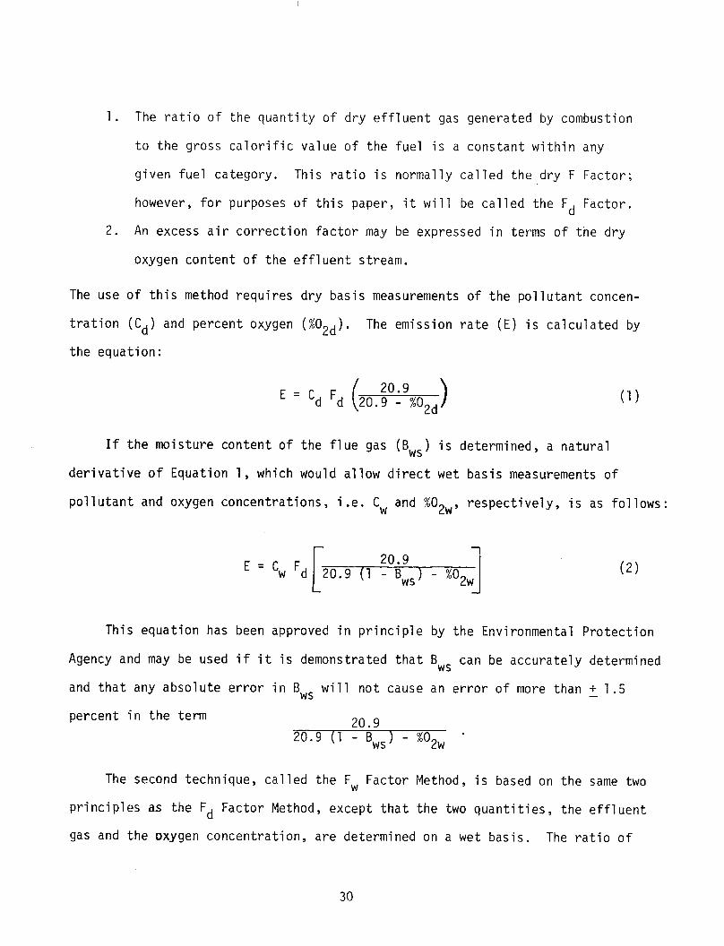
1. The ratio of the quantity of dry effluent gas generated by combustion

to the gross calorific value of the fuel is a constant within any

given fuel category. This ratio is normally called the dry F Factor;

however, for purposes of this paper, it will be called the Fd Factor.

2. An excess air correction factor may be expressed in terms of the dry

oxygen content of the effluent stream.

The use of this method requires dry basis measurements of the pollutant concen-

tration (Cd) and percent oxygen ("02d). The emission rate (E) is calculated by

the equation:

E = Cd

If the moisture content of the

derivative of Equation 1, which wou

pollutant and oxygen concentrations

flue gas (Bws) is determined, a natural

Id allow direct wet basis measurements of

, i.e. Cw and %02w, respectively, is as follows:

Fd 20.9

20.9 - %02d > (1)

E = 'w Fd 20.9

20.9 (1 - Bws) - %02w 1 (2)

This equation has been approved in principle by the Environmental Protection

Agency and may be used if it is demonstrated that Bws can be accurately determined

and that any absolute error in Bws will not cause an error of more than + 1.5 -

percent in the term 20.9 20.9 (1 - Bws) - %Opw *

The second technique, called the Fw Factor Method, is based on the same two

principles as the Fd Factor Method, except that the two quantities, the effluent

gas and the oxygen concentration, are determined on a wet basis. The ratio of

30

. the quantity of wet effluent gas generated by combustion to the gross calorific

value of the fuel is called the wet F Factor or the Fw Factor. The use of this

technique, however, requires in addition to the wet pollutant concentration (Cw)

and oxygen (%02w) the determination of the fractional moisture content of the

air (Bwa) supplied for combustion. (Guidelines for this determination will be

discussed later.) The equation for calculating the emission rate is:

This equation is a simplification of the theoretically derived equation.3 Under

typical conditions, a positive bias of no more than 0.25 percent is introduced.

The third procedure, the Fc Factor Method, is based on principles related

to but slightly different than those for the Fd Factor and F, Factor Methods:

1. For any given fuel category, a constant ratio exists between the volume

of carbon dioxide produced by combustion and the heat content of the

fuel. This ratio is called the Fc Factor.

2. The ratio of the theoretical carbon dioxide produced during combustion

and the measured carbon dioxide provides an exact basis for dilution

correction.

This method requires measurement of the pollutant concentration and percent car-

bon dioxide (%C02) in the effluent stream. Measurements may be made on a wet or

dry basis. Using the subscripts, "d" and "w", to denote dry and wet basis mea-

surements, respectively, the equations for calculating E are:

(4)

37

DETERMINATION OF F FACTORS

Values of Fd in dscf/106 Btu, Fw in wscf/106 Btu, and Fc in scf/106 Btu,

may be determined on an individual case-by-case basis using the ultimate

analysis and gross calorific value of the fuel. The equations are:

Fd = lo6 (3.64 %H + 1.53 %C + 0.57 %S + 0.14 %N - 0.46 %0) GCV (5)

Fw = lo6 (5.57 %H + 1.53 %C + 0.57 %S + 0.14 %N - 0.46 %0 + 0.21 %H20*)

GCVw

Fc = lo ' (0.321 %C) GCV

where: H, C, S, N, 0, and H20 are the concentrations by weight (expressed in

percent) of hydrogen, carbon, sulfur, nitrogen, oxygen, and water from the ulti-

mate analysis. (* Note: The %H20 term may be omitted if %H and %0 include the

unavailable hydrogen and oxygen in the form of H20.) GCV is the gross calorific

value in Btu/lb of the fuel and must always be the value consistent with or

corresponding to the ultimate analysis.

For determining Fw, the ultimate analysis and GCV, must be on an "as received"

or "as fired" basis, i.e., it must include the free water. Often in practice,

the ultimate analysis and/or gross calorific value of a particular fuel are not

known. For most commonly used fuels, tabulated average F Factors may be used in-

stead of the individually determined values. These average values of Fd, Fw, and

FC’ calculated from data obtained from the literature, 2-14 are given in Table I.

F Factors for wood and bark are also listed in Table I, and factors for various

types of refuse are listed in Table II

32

. maximum CO2 concentration that the

this number into 20.9, a ratio cal

culated from the ultimate analyses

II.

The ratio of Fc to Fd times 100 yields the ultimate percent CO2 or the

dry flue gas is able to attain. By dividing

led the F. Factor is obta ined. F. values cal-

of the various fuels are given in Tables I and

F. values can also be calculated from CO2 and O2 data obtained in the field

by using the following equation.

F, = 20.9 - %O*d

%co&, (8)

These calculated F. values can be used to check Orsat data or other analyses of

CO2 and O2 that have been adjusted to a dry basis. The process simply involves

comparing F. values calculated from Equation 8 with the values listed in Table I

or II. Further details of this validation procedure are outlined in Reference 15.

ERRORS AND APPLICATION

ULTIMATE CARBON DIOXIDE

The derivations of Equations 1 through 4 are discussed in References 3, 4,

and 5. The following discussion gives further explanation of the F Factors and

describes some of the problems and errors that arise in applying the F Factor

Methods. Several uses for F Factors in addition to calculating emission rates are

outlined.

Deviation in F Factors

The F Factors were calculated from data obtained from the literature. In

the October 6, 1975, Federal Register,' the values of Fd and Fc were calculated

by summing all data points and

deviat ions from the extreme va

dividing by the total number of samples. Then the

ues (highest and lowest) were determined. The

33

higher of the two values, termed "maximum percent deviation from the average

F Factors," are listed in parenthesis in Table I. These deviations are pro-

bably due to differences in the composition of the fuel, and may also include

variations due to the analytical methods and analysts (laboratories). The stan-

dard deviations of the samples were not calculated since much of the data were

already averages of several samples and there may have been more samples from

one locale or of one kind than another.

After publication of the Fd and Fc Factors, it was determined that the mid-

point value would be a better value than the average for small samples and for

data taken from the literature. Therefore, the Fw Factors and the values for wood

and refuse are midpoint values rather than arithmetic averages. The associated

deviations are termed, "maximum percent deviation from the midpoint F Factor."

Fw Factors for refuse, wood, and wood bark were not calculated because of the

high variability of free moisture contents. For example, the moisture in bark

may vary from 20 percent (air dried) to 75 percent (hydraulic debarking).6 Free

moisture content variations of + 15 percent introduce about 5 percent variation . -

However, for lignite, the moisture contents vary only from about 33 to 45 percent.

This range causes a deviation of 3.8 percent from the midpoint Fw Factor, which

enabled an Fw Factor to be established.

Incomplete Combustion

The assumption of complete combustion is made in the derivation of all

F Factor Methods. If products of incomplete combustion, such as carbon monoxide,

are present in the effluent stream, the volume of effluent gas and carbon dioxide

per pound of fuel burned will differ from the values used in calculating the

F Factors. However, adjustments to the measured CO2 or O2 concentration can be

made, which would minimize the magnitude of the error when applying Equations l-5.

34

These adjustments are given by the following equations:

.

.

("Co~)adj = %C02 + %CO

(%O*)adj = %O* - 0.5 %CO (10)

By making these adjustments, the error amounts to minus one-half the concen-

tration of CO present. Thus, if 1 percent CO (an extreme case) is present, an

error of minus 0.5 percent is introduced. Without adjusting the CO2 or O2 con-

centration, a combustion source having 11 percent CO*, 1 percent CO, and 6 per-

cent O2 will result in about plus 9 percent error for the Fc Factor Method and

about plus 3 percent for the Fd Factor and Fw Factor Methods.

Similarly, unburned combustible matter in the ash will cause the volume of

effluent gas and carbon dioxide per unit of heat input to differ from the calculated

F Factor values. This is true, however, only if the heat input is thought of in

terms of the coal input rate times the calorific value. If the heat input rate is

considered as only that calorific value which is derived from the combusted mat-

ter, the F Factor Methods are only slightly affected. In other words, if any por-

tion of the fuel goes through the combustion process unburned, the F Factor Methods

will not include as heat input the calorific value associated with the uncombusted

matter, and a slight positive bias will be introduced.

The positive bias is due to the combustion process , which is said to consist

first of evaporating the free moisture, then the burning of the volatile matter,

and last the burning of the fixed carbon, with the ash remaining. The volatile

matter includes hydrogen, which results in a lower F Factor than the calculated

values. Since a higher proportion of fixed carbon than volatile matter generally

remains in the ash, the Fc Factor Method is affected more than the Fd Factor and

Fw Factor Methods. For example, assume that 100 lb of a coal, which has

55 8% C, 5.7% H, 1.1% N, 3.2% S, 21.5% 0, and 12.6% ash (percent by weight, as

received basis), is burned and 5 lb fixed carbon remains in the ash. About plus

2.3 percent error is incurred with the Fc Factor and less than 1 percent with the

Fd Factor and Fw Factor Methods.

Effect of Wet Scrubbers

When wet scrubbers are used, a portion of the carbon dioxide may be absorbed

by the scrubbing solution. Therefore, the Fc Factor Method will yield an emission

rate higher than the actual rate. If a gas stream having 14% CO2 before the

scrubber loses 10 percent of the C02, or 1.4% C02, the error is about plus 13 per-

cent.

The Fd Factor Method is also affected by the loss of CO2 in the scrubber,

but to a lesser degree than the Fc Factor Method. If the gas stream has 6% 02 and

1.4% CO2 is lost in the scrubber,,the error will be about plus 2 percent.

The F, Factor Method is not applicable after wet scrubbers since the scrubber

generally adds moisture to the flue gas, thereby "diluting" the gas stream. The

pollutant concentration will be lowered by the same proportion of moisture added

and the O2 concentration will be lower than actual, which would tend to yield lower

than true numbers.

When the scrubbing solution is lime or limestone, the Fc Factor Method may be

used after wet scrubbers. It is generally assumed that due to the optimum operating

conditions, the amount of CO2 absorption is minimized and, therefore, the applica-

tion of the Fc Factor Method will not yield appreciable errors. However, with

limestone scrubbers, there is a possibility of CO2 being added to the gas stream

due to the reaction of SO2 with the limestone. Therefore, the Fc Factors must be

increased by 1 percent.

36

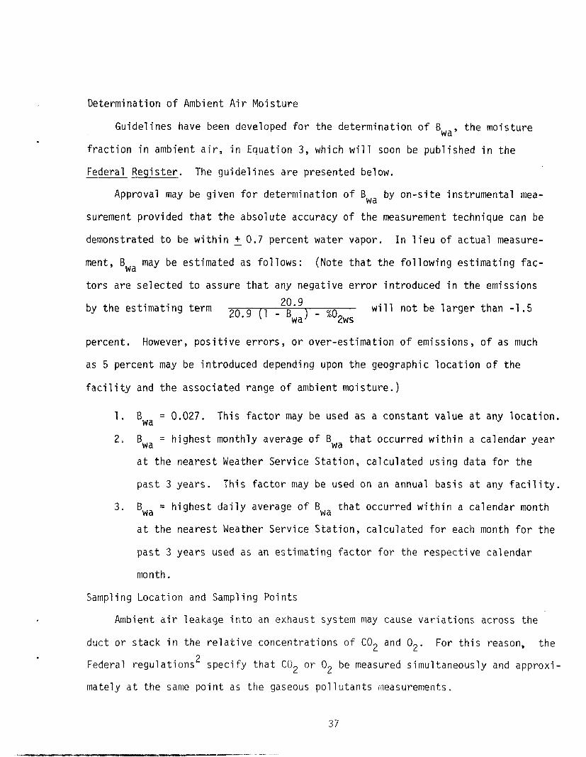
Determination of Ambient Air Moisture

Guidelines have been developed for the determination of Bwa, the moisture

fraction in ambient air, in Equation 3, which will soon be published in the

Federal Register. -- The guidelines are presented below.

Approval may be given for determination of Bwa by on-site instrumental mea-

surement provided that the absolute accuracy of the measurement technique can be

demonstrated ,to be within + 0.7 percent water vapor. In lieu of actual measure-

ment, Bwa may be estimated as follows: (Note that the following estimating fac-

tors are selected to assure that any negative error introduced in the emissions

by the estimating term

percent. However, posi

as 5 percent may be int

20.9 20.9 (1 - Bwa) - %Ozws will not be larger than -1.5

tive errors, or over-estimation of emissions, of as much

reduced depending upon the geographic location of the

facility and the associated range of ambient moisture.)

" Bwa = 0.027. This factor may be used as a constant value at any location.

2* Bwa = highest monthly average of Bwa that occurred within a calendar year

at the nearest Weather Service Station, calculated using data for the

past 3 years. This factor may be used on an annual basis at any facility.

3a Bwa = highest daily average of Bwa that occurred within a calendar month

Sampling

Amb

at the nearest Weather Service Station, calculated for each month for the

past 3 years used as an estimating factor for the respective ca7endar

month.

Location and Sampling Points

ent air leakage into an exhaust system may cause variations across the

duct or stack in the relative concentrations of CO2 and 02. For this reason, the

Federal regulations2 specify that CO2 or O2 be measured simultaneously and approxi-

mately at the same point as the gaseous pollutants measurements.

For particulate emission performance tests, which require traversing, it

is specified that the O2 samples be obtained simultaneously by traversing the

duct at the same sampling location used for each run of the Method 5. This re-

quirement may be satisfied by attaching a stainless steel tube to the particulate

sampling probe and, using a small diaphragm pump, obtaining an integrated gas sam-

ple over the duration of the run (of Reference 1). The sample should be analyzed

using an Orsat apparatus.

As an alternative to traversing the same sampling points of Method 5, a mini-

mum of 12 oxygen sampling points may be used for each run. This would require a

separate integrated gas sampling train traversing the duct work simultaneously

with the particulate run.

Other Applications

In addition to calculating emission rates, F Factors have several other uses.

If= Q,,, the dry effluent volumetric flow rate, or Q,,, the wet effluent volumetric

flow rate, and Q,, the heat input rate, are measured, a value of Fd, Fw, or Fc

may be calculated. These equations are given below:

Q sd

Fd(calc) = $-

20.9 - %02

20.9 (11)

Q sw Fw(calc) = Q,

20.9 (1 - Bwa) - %02w

20.9

F c(calc) --

(12)

(13)

The calculated values may then be compared to tabulated values of the F Factors

to facilitate a material balance check.

38

.

If desired, Q, can be calculated by using the Equations 11 through 13.

In the past, it has been observed that the measurement of Q, has been signifi-

cantly greater than the stoichiometric calculations rates. The discrepancy is

usually due to errors in determining Q,. Due to aerodynamic interferences and

improper alignment of the pitot tubes, higher than real readings have been ob-

tained. Therefore, errors in measuring Q, are positive, which.leads to higher

than true firing rates.

If an ultimate analysis and calorific determination of a particular fuel

are made and the F Factor value is calculated, the accuracy of the results may be

checked by comparison with the tabulated F Factors.

SUMMARY

The various F Factor Methods have been summarized and calculated F Factors

for fossil fuels, wood, wood bark, and refuse material have been presented. In

addition, some of the problems and errors that arise in applying the F Factor

Method for calculating power plant emission rates were discussed and other uses

of the F Factors were outlined.

39

TABLE I. F FACTORS FOR VARIOUS FUELSP-14'aybyc

Fuel Type

Coal

Anthracite

Bituminous

Lignite

Oil

Gas

Natural

Propane

Butane

Wood

Wood Bark

Fd

dscf/106 Btu

10140 (2.0)

9820 (3.1)

9900 (2.2)

9220 (3.0)

8740 (2.2)

8740 (2.2)

8740 (2.2)

9280 (1.9)*

9640 (4.1)

Fw wscf/106 Btu

10580 (1.5)*

10680 (2.7)

12000 (3.8)

10360 (3.5)

10650 (0.8)

10240 (0.4)

10430 (0.7)

-----------

-----------

Fc scf/106 Btu

1980 (4.1) 1.070 (2.9)

1810 (5.9) 1.140 (4.5)

1920 (4.6) 1.076 (2.8)

1430 (5.1) 1.346 (4.1)

1040 (3.9) 1.749 (2.9)

1200 (l.o)* 1.510 (1.2)*

1260 (1.0) 1.479 (0.9)

1840 (5.0)

1860 (3.6)

FO -

1.050 (3.4)

1.056 (3.9)

a Numbers in parenthesis are maximum deviations (%) from either the midpoint or average F Factors.

b To convert to metric system, multiply the above values by 1.123 x 10e4 to obtain

scm/106 cal.

' All numbers below the asterisk (*) in each column are midpoint values. All others are averages.

TABLE II. MIDPOINT F FACTORS FOR REFUSE2-14Yayb

Paper and Wood WastesC

Lawn and Garden Wastesd

Plastics

Polyethylene

Polystyrene

Polyurethane

Polyvinyl chloride

Garbagee

Miscellaneous

Citrus rinds and seeds

Meat scraps, cooked

Fried fats

Leather shoe

Heel and sole composition

Vacuum cleaner catch

Textiles

Waxed milk cartons

Fd

dscf/lO'Btu

9260 (3.6)

9590 (5.0)

9173 1380 1.394

9860 1700 1.213

10010 1810 1.157

9120 1480 1.286

9640 (4.0) 1790 (7.9) 1.110 (5.6)

9370

9210

8939

9530

9480

9490

9354

9413

FC

wscf/106Btu

1870 (3.3)

1840 (3.0)

1920

1540

1430

1720

550

700

840

620

FO

1.046(4.6)

1.088 (2.4)

1.020

1.252

1.310

1.156

1.279

1.170

1.060

1.040

a Numbers in parentheses are maximum deviations (%) from the midpoint F Factors.

b To conltert to metric system, multiply the above values by 1.123 x 10B4 to obtain ‘ scm/lO cal.

l ' Includes newspapers, green logs,

brown paper, corrugated boxes, magazines, junk mail, wood, rotten timber.

d Includes evergreen shrub cuttings, flowing garden plants, leaves, grass.

e Includes vegetable food wastes, garbage (not described).

41

REFERENCES

1. Standards of Performance for New Stationary Sources. Federal Register.

36:247, Part II. December 23, 1971. -

2. Requirements for Submittal of Implementation Plans and Standards for New

Stationary Sources. Federal Register. 40:194, Part V. October 6, 1975.

3. Shigehara, R. T. and R. M. Neulicht. Derivation of Equations for Calculating

Power Plant Emission Rates, O2 Based Method - Wet and Dry Measurements. Emis-

sion Measurement Branch, ESED, OAQPS, U. S. Environmental Protection

Agency, Research Triangle Park, N.C. July 1976.

4. Shigehara, R. T., R. M. Neulicht, and W. S. Smith. A Method for Calculating

Power Plant Emissions. Stack Sampling News. 1 (1):5-g. July 1973.

5. Neulicht, R. M. Emission Correction Factor for Fossil Fuel-Fired Steam Genera-

tors: CO2 Concentration Approach. Stack Sampling News. 2 (8);6-11. February 1975.

6. Fuels, Distribution, and Air Supply. In: C-E Bark Burning Boilers (Sales

Brochure). Windsor, Conn., Combustion Engineering Inc. p.5.

7. Kaiser, E. R. Chemical Analyses of Refuse Components. In: Proceedings of 1966

National Incinerator Conference. The American Society of Mechanical Engineers,

1966. p.84-88.

8. Kaiser, E. R., C. D. Zeit, and J. B. McCaffery. Municipal Refuse and Residue.

In: Proceedings of 1968 National Incinerator Conference. The American Society

of Mechanical Engineers, 1968. p.142-152.

9. Kaiser, E. R. and A. A. Carrotti. Municipal Refuse with 2% and 4% Addition of

Four Plastics: Polyethylene, Polyurethane, Polystyrene, and Polyvinyl Chloride.

In: Proceedings of 1972 National Incinerator Conference. The American Society

of Mechanical Engineers, 1972. p.230-244.

42

10. Kaiser, E. R. The Incineration of Bulky Refuse. In: Proceedings of 1966

National Incinerator Conference. The American Society of Mechanical Engineers,

1966. p.39-48.

11. Newman, L. L. and W. H. Ode. Peat, Wood, and Miscellaneous Solid Fuels. In:

Mark's Standard Handbook for Mechanical Engineers, Baumeister, T. (ed.).

7th ed. New York, McGraw-Hill Book Company, 1967. Chapter 7, p.19.

12. MacKnight, R. J. and J. E. Williamson. Incineration: General Refuse Incinera-

tors. In: Air Pollution Engineering Manual, Danielson, J. A. (ed.). 2nd ed.

OAWM, OAQPS, U. S. Environmental Protection Agency, Research Triangle Park,

N. C. AP-40. May 1973. p.446.

13. Steam, Its Generation and Use. 37th ed. New York, the Babcock and Wilcox

Company, 1963. Appendix 3-A4.

14. The Ralph M. Parsons Company. Solid Waste Disposal System, Chicago. Vol. II

Study Report Appendices. Prepared for Bureau of Engineering, Department of

Public Works, City of Chicago. May 1973.

15. Shigehara, R. T., R. M. Neulicht, and W. S. Smith. Validating Orsat Analysis

Data from Fossil Fuel-Fired Units. Emission Measurement Branch, ESED, OAQPS,

U. S. Environmental Protection Agency, Research Triangle Park, N. C. June 1975.

43

VALIDATING ORSAT ANALYSIS DATA FROM FOSSIL-FUEL-FIRED UNITS

R. T. Shigehara, R. M. Neulicht, and W. S. Smith

INTRODUCTION

In the September 11, 1974 Federal Register,' a new reference method

for calculating the pollutant emissions from fossil fuel-fired steam -

generating units of more than 250 million Btu/hr heat input was proposed.

This proposed method is based on the law of conservation of mass and energy

and utilizes oxygen (02) concentration to compensate for excess or dilution

air. 2 Recently, another method has been published3 that uses the same prin-

ciple, except that carbon dioxide (C02) concentration is used to adjust for

excess or dilution air.

The validity of both methods relies heavily on the accuracy of either

the O2 or CO2 measurement. Therefore, it is desirable to have some criteria

for validating the data as soon as they are obtained in the field. Since,

in many cases, both O2 and CO2 measurements are obtained from Orsat analyses,

guidelines are given for validating the data from these analyses.

C02-O2 RELATIONSHIP

Since air is used for the combustion process, the law of conservation

of mass demands that:

%02 + F. %C02 = 20.9 (1)

where: %02 = O2 content by volume (expressed as percent), dry basis

%C02 = CO2 content by volume (expressed as percent), dry basis

F. = fuel factor; depends on the type of fuel burned

20.9 = O2 content in air by volume (expressed as percent), dry basis.

Publirilcd in 5tacb .'arwlinc '1~5 /1(Z): ?1 -?f- , "un115t "'76 . 44

Solving for Fo, we obtain:

20.9 F. =

- %02

%CO* (2)

The factor F. is mainly a function of the hydrogen (H) to carbon (C) ratio

in the fuel.4 At zero percent excess air (i.e., when fuel is burned com-

pletely with stoichiometric amount of air), Equation 2 simplifies to:

F. = * (3)

where (%C02)ult is the ultimate CO2 or the maximum CO2 concentration that

the dry flue gas is able to attain. Given the ultimate analysis of the fuel

being burned, this value can be calculated by using the following equation:5

wo2)ul t = 0.321 %C (100) 1.53 %C + 3.64 XH + 0.57 %S + 0.14 %N - 0.46 %0 (4)

where %C, %H, %S, %N, and %0 are the percent by weight of carbon, hydrogen,

sulfur, nitrogen, and oxygen, respectively, obtained from the ultimate

analysis.

Equations 1 through 4 can be used to check Orsat data or other analyses

of CO2 and O2 that have been adjusted to a dry basis. The process simply in-

volves comparing F. values calculated from Orsat analyses (Equation 2) with

F. values calculated from the ultimate analyses of the fuels being burned

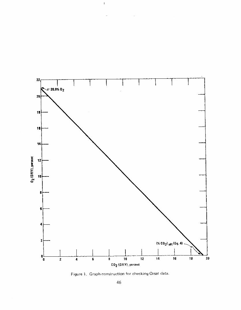
(Equations 3 and 4). Alternatively, a graphical approach may be used. With

CO2 as the abscissa and O2 as the ordinate on arithmetic paper (see Figure 1),

a straight line drawn between 20.9% O2 and the ultimate CO2 calculated from

the ultimate analysis (Equation 4) represents Equation 1. The Orsat analysis

4.5

16 -

14 -

B-

6-

CO2 (DRY), percent

Figure 1. Graph construction for checking Orsat data.

46

is checked by plotting the data points on this graph.

Equation 1 or 2 assumes complete combustion of the fuel. If carbon

monoxide (CO) is present in measurable quantities, the O2 and CO 2 must be

adjusted when using the equations as follows:

(%"2)adj = %C02 + %CO

(%02)adj = %02 - 0.5 %CO (6)

(5)

Since the method of validating Orsat analyses is based on combustion

of fossil fuel and dilution of the gas stream with air, this method will not

be applicable to sources that (1) remove CO2 (e.g., sources that use wet

scrubbers) or 02, or (2) add O2 and N2 in a proportion different from that

of air or (3) add CO2 (e.g., cement kilns).

SUMMARY OF AVERAGE F. FACTORS AND ULTIMATE C02'S

When ultimate analyses of the fuel being burned are not available,

averages may be used. Table I summarizes F. factors and ultimate C02's and

their averages for various type fuels based on ultimate analyses reported in

the literature. 6-15 Some of the average F, factors and (%COp)ult were cal-

culated by use of a small number of samples. It is recommended, therefore,

that the data be updated by users as more information becomes available. The

manner in which these averages can be used to validate Orsat data will be ex-

plained later.

F, and ULTIMATE CO2 TOLERANCES

As mentioned earlier, the purpose for the O2 or CO2 measurements is

primarily to adjust the pollutant concentrations for dilution air. In

47

Table I Fo Factors for Fossil Fuelsa

Literature Number of Average Maximum Deviation, % Fuel type source samples FO

(% co*)u,t +

Coal

Anthracite

Overall avg.

Bituminous

Overall avg.

Lignite

Overall avg.

Oil

Crude

Residium

Distillate

Overall avg.

Gas

Natural

Overall avg.

Propane

Overall avg.

Butane

Overall avg.

6 3

7 1

8 3

8 13

9 38

10 13

11 39

12 26

8 1

6 1

16 198

7 1

14 6

14 4

14 2

15

6

15

15

1.0786 19.38

1.0525 19.86

1.0671 19.59

1.0699 19.53

1.1202 18.66

1.1407 18.32

1.1336 18.44

1.1450 18.25

1.1435 18.28

1.1398 18.34

1.0779 19.39

1.0791 19.37

1.0761 19.42

1.0761 19.42

1.3628 15.34

1.3561 15.41

1.3280 15.74

1.3464 15.52

1.3465 15.52

1.7594

1.7349

1.7489

1.5095

1.5095

1.4791

1.4791

11.88

12.05

11.95

13.85

13.85

14.13

14.13

2.9 2.3

3.6 4.5

2.8 2.8

2.9

1.8

1.2

0.9

4.1

2.9

1.2

0.9

a Standard conditions are 7O"F, 29.92 in. Hg, and 0% excess air.

48

evaluating the effect of the inaccuracy of the measurement on the final

result, it is important to consider not only the 02 and CO2 relationship,

but also the level of their concentrations. An explanation follows.

The adjustment factors for dilution air are:

Fdo =

20.9 - K.

20.9 - %02

KC Fdc = - %C02

(7)

(8)

where: Fdo and Fdc = adjustment factors for dilution air based on O2 and

C02, respectively

K. and Kc = reference O2 and CO2 concentrations, respectively

%02 and %C02 = percent by volume of O2 and CO2, respectively, dry basis

20.9 = percent by volume of O2 in air, dry basis.

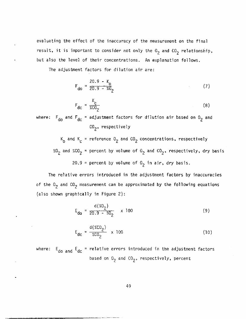
The relative errors introduced in the adjustment factors by inaccuracies

of the O2 and CO2 measurement can be approximated by the following equations

(also shown graphically in Figure 2):

Edo =

d(%02)

20.9 - %O* x 100 (9)

d(%C02)

Edc = %CO2 x 100 (10)

where: Edo and Edc = relative errors introduced in the adjustment factors

based on 02 and C02, respectively, percent

49

I I 2.4 -

1 I I I

-,1.6+- 170* 0‘

g 0.8 a t- a Ly

I

0.6 i--- / /

I 0 2 4 6 8 10 12 14 16 18

LEVEL OF CO2 OR 02, percent

Figure 2. Relative errors resulting from inaccurate CO2 or 02 measurements.

50

.

d(%02) and d(%C02) = deviation from the true value of O2 and COz, respec-

tively, percent by volume.

If d(%02)'s and d(%C02)'s can be determined or estimated, Figure 2

can be valuable in making decisions or evaluations. For example, if the

CO2 level is about 12 to 14%, Fyrites * that are capable of measuring CO2 to

within 0.5% would be adequate for making Fdc calculations. If the CO2 con-

centration is down at the 2% level, however, it can be seen that to achieve,

for example, a 5% accuracy, a measurement to within 0.1% CO2 is required.

Thus, Orsats tiith burettes capable of measuring to within 0.1% C02, not

Fyrites, should be used.

To estimate the tolerances of F. and the ultimate CO2 for a desired

accuracy of Ed0 or Edc, the following relationship is helpful:

dFO -= d(%C02)ul t _

i

d(%O&

FO (%co2)u, t

- - 20.9 - %O* -

Equation 11 shows that the tolerance of F. or (%C02)ult is the sum of

Edo and Edc. With the understanding that Ed0 and Edc can be a range of plus

or minus values, however, the tolerance of F. or (%C02)u,t must be-limited to

the same magnitude of Ed0 or Edc to ensure that Ed0 or Edc will be less than

that magnitude. For example, to limit Ed0 or Edc to + 5%, F. or (%C02)ult -

must also be limited to + 5%.

PROCEDURE

.

Based on the previous discussion, the following procedure can be

established for validating Orsat analysis data:

rTrade name; not to be considered an endorsement.

1. Decide tolerances for Ed0 or Edc.

2. If ultimate analysis of fuel being burned is available, calculate

F. using Equations 3 and 4 or (%C02)ult using Equation 4. Otherwise, use

average values from Table I. Then calculate the limits of tolerance for

F. or (%C02)ult. For example, if a 5 5% tolerance is desired, the tolerance

limits would be 0.95 and 1.05 times the calculated F, or (% C02) ult. Con-

struct graphs as in Figure 1, using these tolerance limits.

3. To compare field Orsat data, calculate Fo, using Equation 2, or

plot the data points on the graph. Values beyond the established tolerance

levels should be rejected and the analysis run over.

If average values, rather than the ultimate analysis of the fuel being

burned, serve as the basis of comparison, it should be understood that there

may be exceptions. If repeated Orsat analyses, including a double-check of

the Orsat apparatus and analyses run by another person, consistently yield

values that are rejected, the average values should be considered suspect

and the Orsat analyses accepted.

A graphical nomograph technique using a 5 5% tolerance level and average

values from Table I is shown in Figure 3.

SUMMARY

For any given fuel burned with air, a relationship between O2 and CO2

must exist. This relationship can be used to advantage to validate Orsat

analysis data. On the basis of ultimate analysis or average values of F. or

myu,t ca?culated from data in the literature, a procedure has been pre-

sented for validating Orsat analysis data.

52

ANTHRACITE, LIGNITE

NATURAL GAS

Figure 3. Nomograph for checking Orsat data t 5% in Ed0 or Edc.

53

REFERENCES

1. Federal Register, Proposed Emission Monitoring and Performance

Testing Requirements for New Stationary Sources, 39:177, Part 11

(September 11, 1974).

2. Shigehara, R. T., Neulicht, R. M., and Smith, W. S., "A Method

for Calculating Power Plant Emission Rates," Stack Sampling News, July,

1973, Volume 1, Number 1, p. 5-9.

3. Neulicht, R. M., "Emission Correction Factor for Fossil Fuel-

Fired Steam Generators: CO2 Concentration Approach," Stack Sampling News,

February, 1975, Volume 2, Number 8, p. 6-11.

4. DeVorken, H., Chass, R. L., and Fudurich, A. P., "Air Pollution

Source Testing Manual," APCD, County of Los Angeles (1972), p. 96.

5. North American Combustion Handbook, North American Manufacturing

Company, Cleveland (1965), p. 48.

6. Perry, John H., ed., Chemical Engineers' Handbook, 4th ed., McGraw

Hill Book Company, N. Y. (1963), p. 9-3.

7. North American Combustion Handbook, North American Manufacturing


8. Steam, The Babcox and Wilcox Company, New York (1963), p. Z-10.

9. Analysis of Tipple and Delivered Samples of Coal, U. S. Dept. of

Int., U. S. Bureau of Mines, Washington, D. C., Publication No. USBMRI

7588 (1972).

10. U. S. Dept. of Interior, U. S. Bureau of Mines, Washington, D. C.,

Publication No. USBMRI 7490 (1971).

54




Publication No. USBMRT 7219 (1969).



14. North American Combustion Handbook, North Anerica,Manufacturing




55

A GUIDELINE FOR EVALUATING COMPLIANCE TEST RESULTS

(Isokinetic Sampling Rate Criterion)

R. T. Shigehara Emission Measurement Branch, ESED, OAQPS, EPA

Introduction

The sampling rate used in extracting a particulate matter sample

is important because anisokinetic conditions can cause sample concentra-

tions to be positively or negatively biased due to the inertial effects

of the particulate matter. Hence, the calculation of percent isokinetic

(I) is a useful tool for validating particulate test results. Section 6.12

of the recently revised Method 5' states, “If 90 percent 5 I 2 110 percent,

the results are acceptable. If the results are low in comparison to the

standard and I is beyond the acceptable range, or, if I is less than

90 percent, the Administrator may opt to accept the results."

This guideline provides a more detailed procedure on how to use

percent isokinetic to accept or reject test results when the sampling rate

is beyond the acceptable range. The basic approach of the procedure is to

account for the inertial effects of particulate matter and to make a n

maximum adjustment on the measured particulate matter concentration.L Then,

after comparison with the emission standard, the measured particulate matter

concentration is categorized (1) as clearly meeting or exceeding the

emission standard or (2) as being in a "gray area" zone. In the former

category, the test report is accepted; in the latter, a retest should

be done because of anisokinetic sampling conditions.

Procedure

1. Check or calculate the percent isokinetic (I) and the particulate

Published in Source Evaluation Society Newsletter Z(3), August 1977

56

matter concentration (cs) according to the procedure outlined in Method 5.

Note that cs must be calculated using the volume of effluent gas actually

sampled (in units of dry standard cubic feet, corrected for leakage).

Calculate the emission rate (E), i.e. convert cs to the units of the

standard. For the purposes of this guideline, it is assumed that all

inputs for calculating E are correct and other specifications of Method 5

are met.

2. Compare E to the standard. Then accept or reject cs using the

criteria outlined below. (A summary is given in Table I):

a. Case 1 - I is between 90 and 110 percent. The concentration

cs must be considered acceptable. A variation of + 10 percent from 100

percent isokinetic is permitted by Method 5.

b. Case 2 - I is less than 90 percent.

(1) If E meets the standard, cs should be accepted, since

cs can either be correct (if all particulate matter are less than about 5

micrometers in diameter) or it can be biased high (if larger than 5

micrometer particulate matter is present) relative to the true concentration;

one has the assurance that cs is yielding an E which is definitely below

the standard.

(2) If E is above the standard, multiply cs by the factor

(I/100) and recalculate E. If, on the one hand, this adjusted E is still

higher than the standard, the adjusted cs should be accepted; a maximum

adjustment which accounts for the inertial effects of particulate matter

has been made and E still exceeds the standard. On the other hand, if the

57

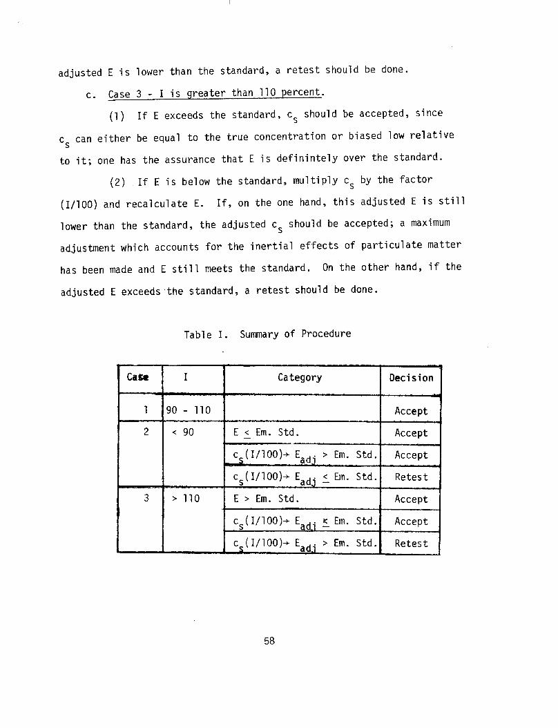
adjusted E is lower than the standard, a retest should be done.

C. Case 3 - I is greater than 110 percent.

(1) If E exceeds the standard, cs should be accepted, since

cs can either be equal to the true concentration or biased low relative

to it; one has the assurance that E is definintely over the standard.

(2) If E is below the standard, multiply cs by the factor

(I/100) and recalculate E. If, on the one hand, this adjusted E is still

lower than the standard, the adjusted cs should be accepted; a maximum

adjustment which accounts for the inertial effects of particulate matter

has been made and E still meets the standard. On the other hand, if the

adjusted E exceeds.the standard, a retest should be done.

Table I. Summary of Procedure

E > Em. Std.

58

Summary

.

A procedure for accepting or rejecting particulate matter test

results based on pcvzent isokinetic has been outlined. It provides a

mechanism for accepti:lg all data except where anisokinetic sampling

might affect the validity of the test results. This procedure is one

of several useful tools for evaluating testing results.

References

1. Method 5 - Determination of Particulate Emissions from Stationary

Sources. Federal Register. 42(160):41776-41782, August 18, 1977. -

2. Smith, W. S., R. T. Shigehara, and W. F. Todd. A Method for

Interpreting Stack Sampling Data. Stack Sampling News. 'l-(2):8-17,

August 1973.

Koger T. Shigehara (Editor) _-__--- ----- ~---~- ..-_ ~~ ~- --.-

~%RFORMING ORGANIZATION NAME AND ADDRESS ~_~.--- -- ~~p-~-~~~~MLLEM~~~‘N~~.-. ~-___~ -

U.S. Environmental Protection Agency Emission Standards and Engineering Division (._----F_-.----~

,ll. CONTRACT/GRANT NO

Emission Measurement Branch Research Triangle Park, NC 27711

-__-_.~---- ____ - 2. SPONSORING AGENCY NAME AND ADDRESS

--__--- - ----..__ ._ ___.

t

13. TYPE OF REPORT AND PERIOD COVEREO

Same as above.

5. SUPPLEMENTARY NOTES

-I 6. ABSTRACT

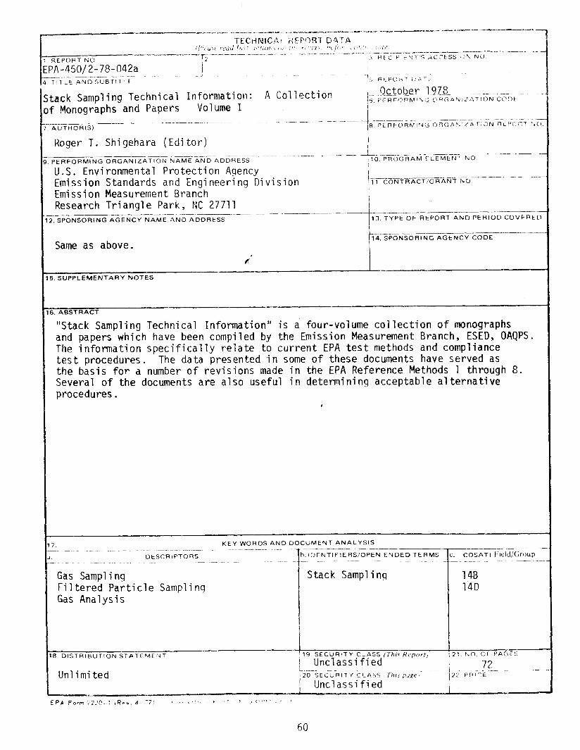
"Stack Sampling Technical Information" is a four-volume collection of monographs and papers which have been compiled by the Emission Measurement Branch, ESED, OAQPS. The information specifically relate to current EPA test methods and compliance test procedures. The data presented in some of these documents have served as the basis for a number of revisions made in the EPA Reference Methods 1 through 8. Several of the documents are also useful in determining acceptable alternative procedures.

_

Gas Sampling Filtered Part i Gas Analysis

KEY WORDS AND DOCUMENT ANALYSIS __ .._~~ ~-~~. --~~----~--- -

DESCRIPTORS b.iUENTIFlERSi’OPEN ENDED TERMS _ _ -. ~~ ~~~

cle Sampling Stack Sampling

--- 8 DISTRIBUTION STPlIL*ltrdT ! 19 SECURITY -CLnSS /77i1r- Kc’porf,

/ Unclassified Unlimited

i

14B 14D

! 1 Iv 0. CJ F PA c, E !:

72

EPA Form ,.22P..: ,RcY, 4.-,-i’ j ,ii \ :. F ‘1 I :, ,,-> !I r , 6 ‘

60

Documents

Stack Sampling Technical Information: A Collection of ... · between the fuel heat value and dry effluent that permits a constant (F Factor ... The method calculating emission rates