STABLE NON-GAUSSIAN ASSET ALLOCATION:A COMPARISON WITH THE CLASSICAL GAUSSIAN APPROACH

Yesim Tokat,Svetlozar Rachev, and Eduardo Schwartz

I. Introduction

Strategic investment planningStochastic programming with and

without decision rulesCharacteristics of financial and

macro data: heavy tails, time varying volatility and long-range dependence

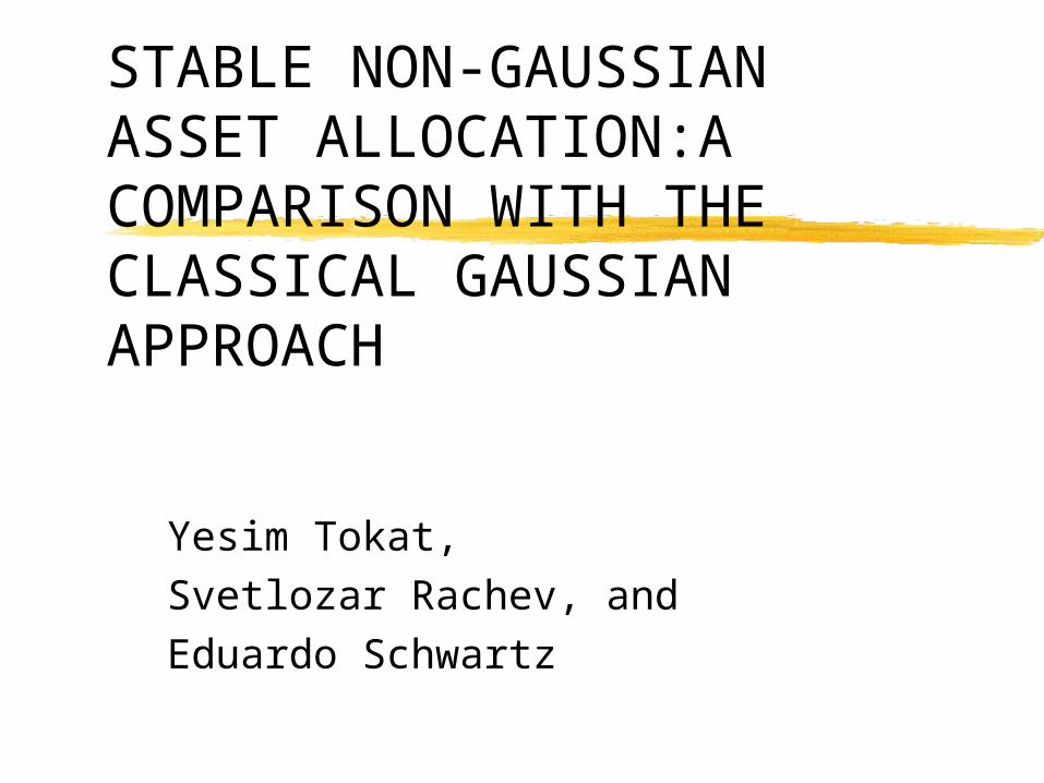
I. Introduction

Generate economic scenarios under Gaussian and stable Paretian non-Gaussian assumptions

Different allocations depending on the utility function and the risk aversion level of the agent very low or high risk aversion ‘typical’ risk aversion

II. Multistage Stochastic Programming with Decision Rules

Discretize time into n stages, and use a decision rule at each time period

Boender et al. (1998):ALM model for pension funds

randomly generate initial asset mixessimulate against generated scenariosevaluate downside risk and contribution

rate

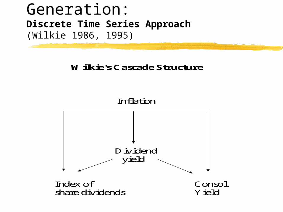
Wilkie's Cascade Structure

Inflation

Dividend yield

Index of Consolshare dividends Yield

III. Scenario Generation:Discrete Time Series Approach (Wilkie 1986, 1995)

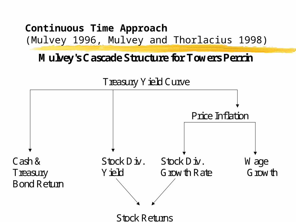
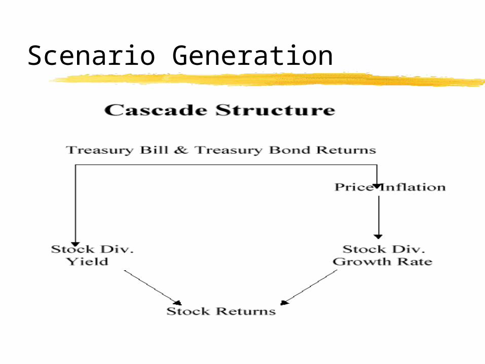
Mulvey's Cascade Structure for Towers Perrin

Treasury Yield Curve

Price Inflation

Cash & Stock Div. Stock Div. WageTreasury Yield Growth Rate GrowthBond Return

Stock Returns

Continuous Time Approach (Mulvey 1996, Mulvey and Thorlacius 1998)

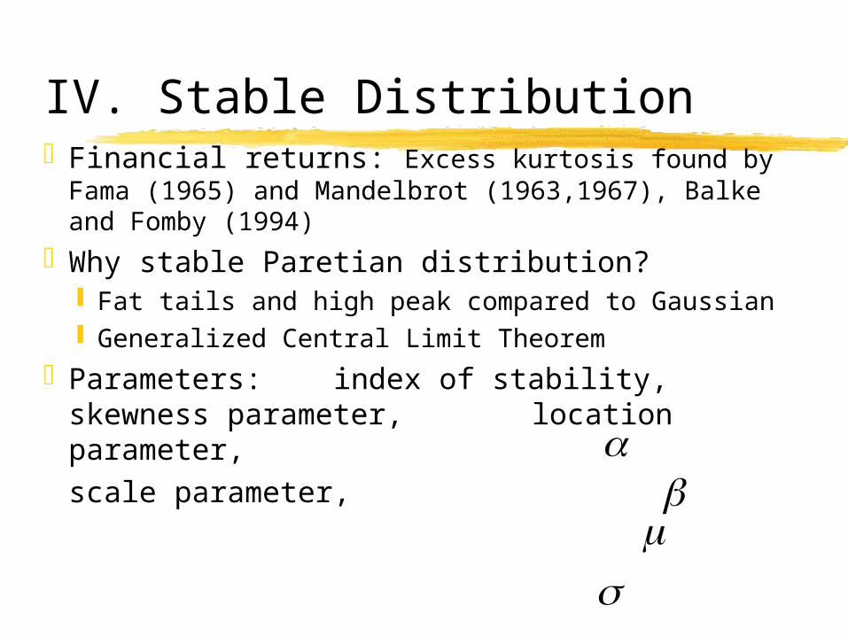
IV. Stable DistributionFinancial returns: Excess kurtosis found by Fama

(1965) and Mandelbrot (1963,1967), Balke and Fomby (1994)

Why stable Paretian distribution? Fat tails and high peak compared to Gaussian Generalized Central Limit Theorem

Parameters: index of stability, skewness parameter,

location parameter, scale parameter,

V. Model Setup

Asset allocation generate initial asset allocations (a fixed

mix) simulate future economic scenarios update asset allocation every month

using fixed mix rule calculate the risk and reward choose initial mix that gives the best risk-

reward combination

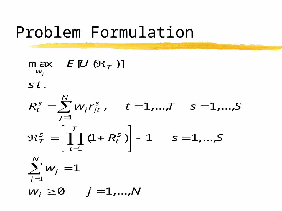
Problem Formulation

1

1

1

max [ ( )]

. .

, 1,..., 1,...,

(1 ) 1 1,...,

1

0 1,...,

jT

w

Ns st j jt

j

Ts sT t

t

N

jj

j

E U

s t

R w r t T s S

R s S

w

w j N

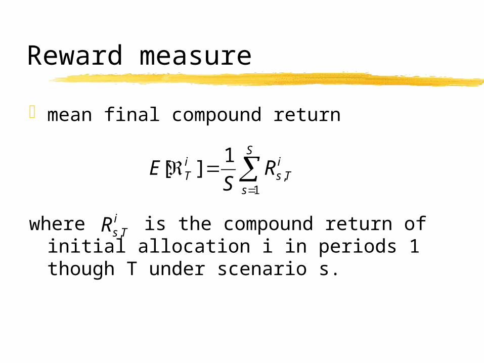
Reward measure

mean final compound return

where is the compound return of initial allocation i in periods 1 though T under scenario s.

S

s

iTs

iT R

SE

1,

1][

iTsR ,

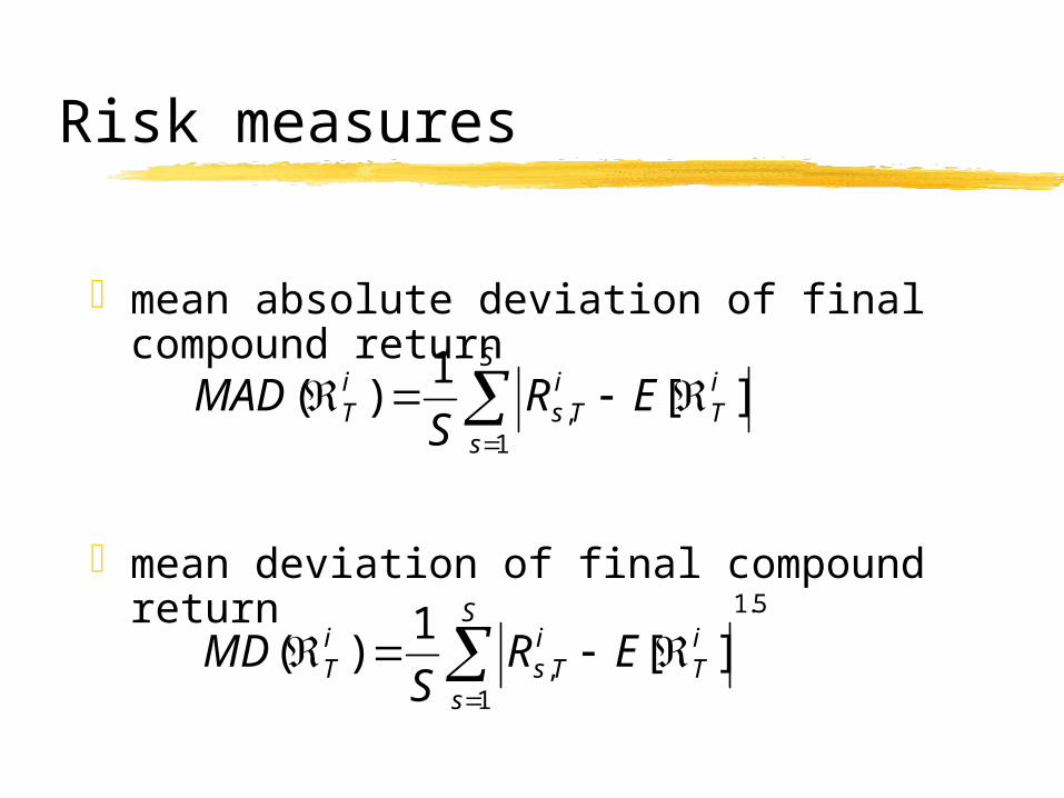
Risk measures

mean absolute deviation of final compound return

mean deviation of final compound return

S

s

iT

iTs

iT ER

SMAD

1, ][

1)(

5.1

1, ][

1)(

S

s

iT

iTs

iT ER

SMD

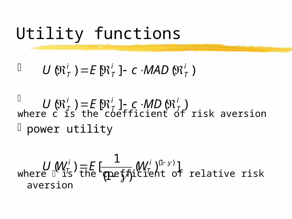
Utility functions

where c is the coefficient of risk aversionpower utility

where is the coefficient of relative risk aversion

)(][)( iT

iT

iT MADcEU

)(][)( iT

iT

iT MDcEU

])()1(

1[)( )1(

i

TiT WEWU

Scenario Generation

Scenario Generation

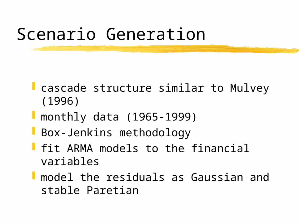
cascade structure similar to Mulvey (1996)

monthly data (1965-1999) Box-Jenkins methodology fit ARMA models to the financial variables model the residuals as Gaussian and

stable Paretian

Scenario Generation

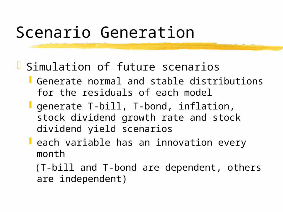
Simulation of future scenarios Generate normal and stable distributions for

the residuals of each model generate T-bill, T-bond, inflation, stock

dividend growth rate and stock dividend yield scenarios

each variable has an innovation every month (T-bill and T-bond are dependent, others are

independent)

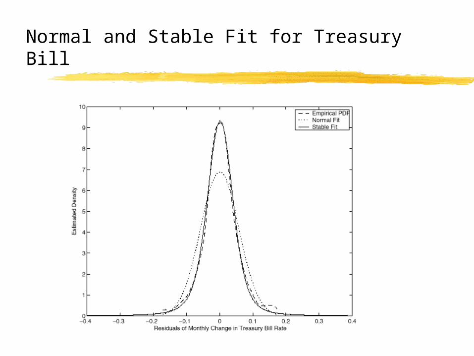
Normal and Stable Fit for Treasury Bill

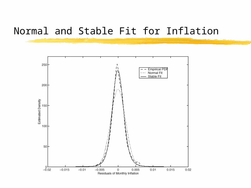
Normal and Stable Fit for Inflation

Normal and Stable Fit for Dividend Growth

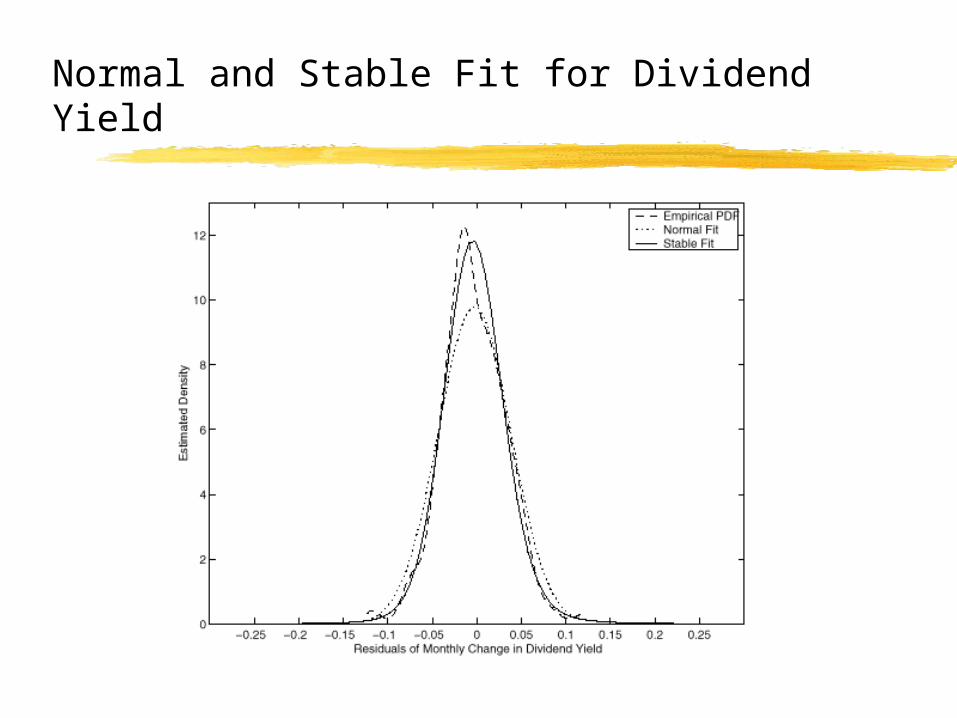
Normal and Stable Fit for Dividend Yield

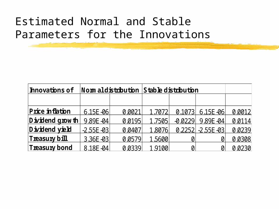
Estimated Normal and Stable Parameters for the Innovations

Innovations of Normal distribution Stable distribution

Price inflation 6.15E-06 0.0021 1.7072 0.1073 6.15E-06 0.0012Dividend growth 9.89E-04 0.0195 1.7505 -0.0229 9.89E-04 0.0114Dividend yield -2.55E-03 0.0407 1.8076 0.2252 -2.55E-03 0.0239Treasury bill 3.36E-03 0.0579 1.5600 0 0 0.0308Treasury bond 8.18E-04 0.0339 1.9100 0 0 0.0230

Simulation

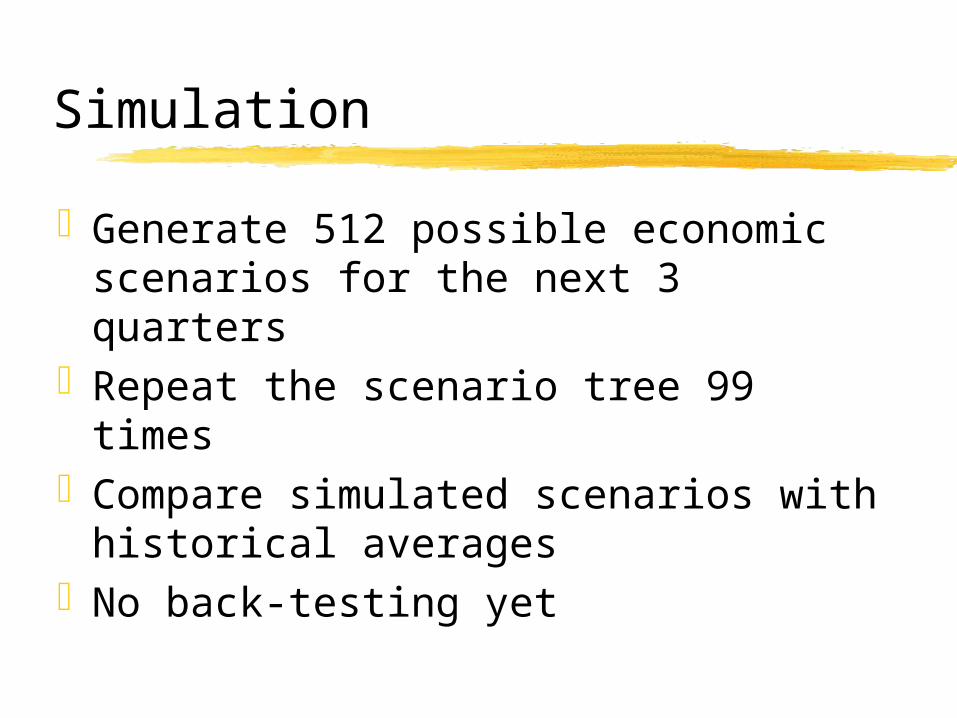
Generate 512 possible economic scenarios for the next 3 quarters

Repeat the scenario tree 99 timesCompare simulated scenarios with

historical averagesNo back-testing yet

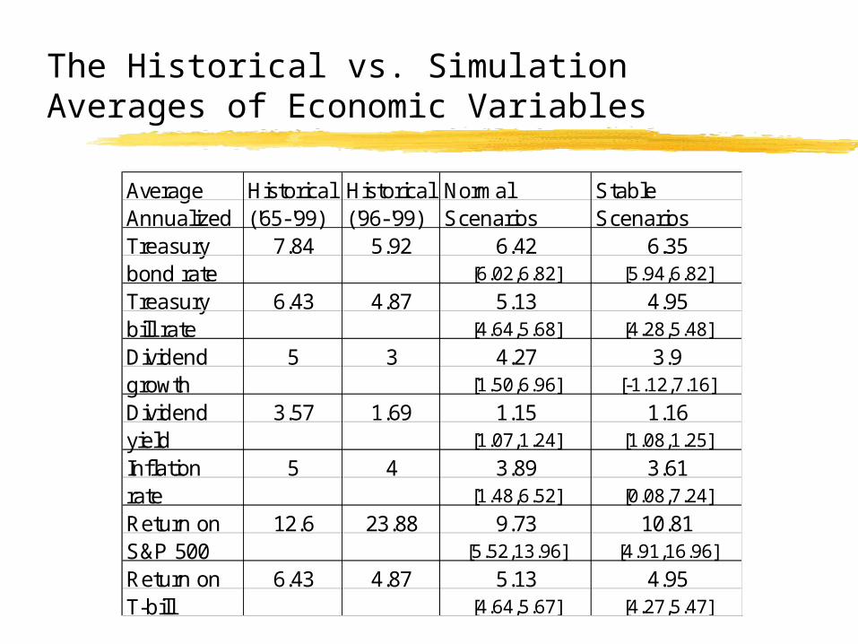
The Historical vs. Simulation Averages of Economic Variables

Average Historical Historical Normal StableAnnualized ('65-'99) ('96-'99) Scenarios ScenariosTreasury 7.84 5.92 6.42 6.35bond rate [6.02,6.82] [5.94,6.82]

Treasury 6.43 4.87 5.13 4.95bill rate [4.64,5.68] [4.28,5.48]

Dividend 5 3 4.27 3.9growth [1.50,6.96] [-1.12,7.16]

Dividend 3.57 1.69 1.15 1.16yield [1.07,1.24] [1.08,1.25]

Inflation 5 4 3.89 3.61rate [1.48,6.52] [0.08,7.24]

Return on 12.6 23.88 9.73 10.81S&P 500 [5.52,13.96] [4.91,16.96]

Return on 6.43 4.87 5.13 4.95T-bill [4.64,5.67] [4.27,5.47]

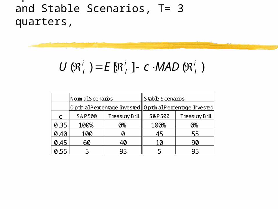
Optimal Allocations under Normal and Stable Scenarios, T= 3 quarters,

Normal Scenarios Stable Scenarios

Optimal Percentage Invested Optimal Percentage Invested

c S&P500 Treasury Bill S&P500 Treasury Bill

0.35 100% 0% 100% 0%0.40 100 0 45 550.45 60 40 10 900.55 5 95 5 95

)(][)( iT

iT

iT MADcEU

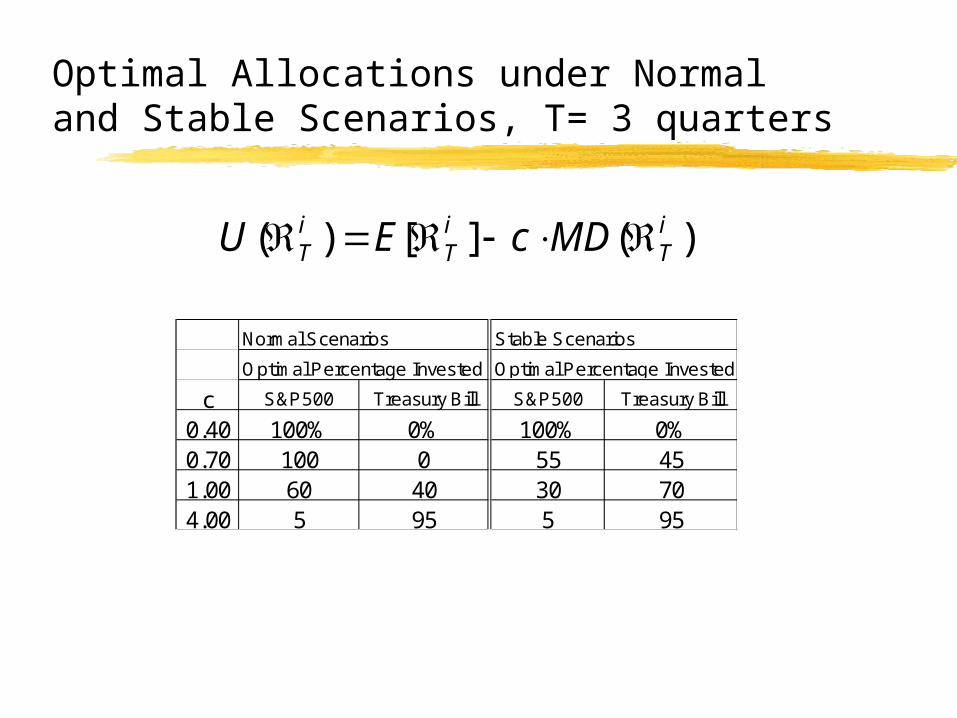
Optimal Allocations under Normal and Stable Scenarios, T= 3 quarters

Normal Scenarios Stable Scenarios

Optimal Percentage Invested Optimal Percentage Invested

c S&P500 Treasury Bill S&P500 Treasury Bill

0.40 100% 0% 100% 0%0.70 100 0 55 451.00 60 40 30 704.00 5 95 5 95

)(][)( iT

iT

iT MDcEU

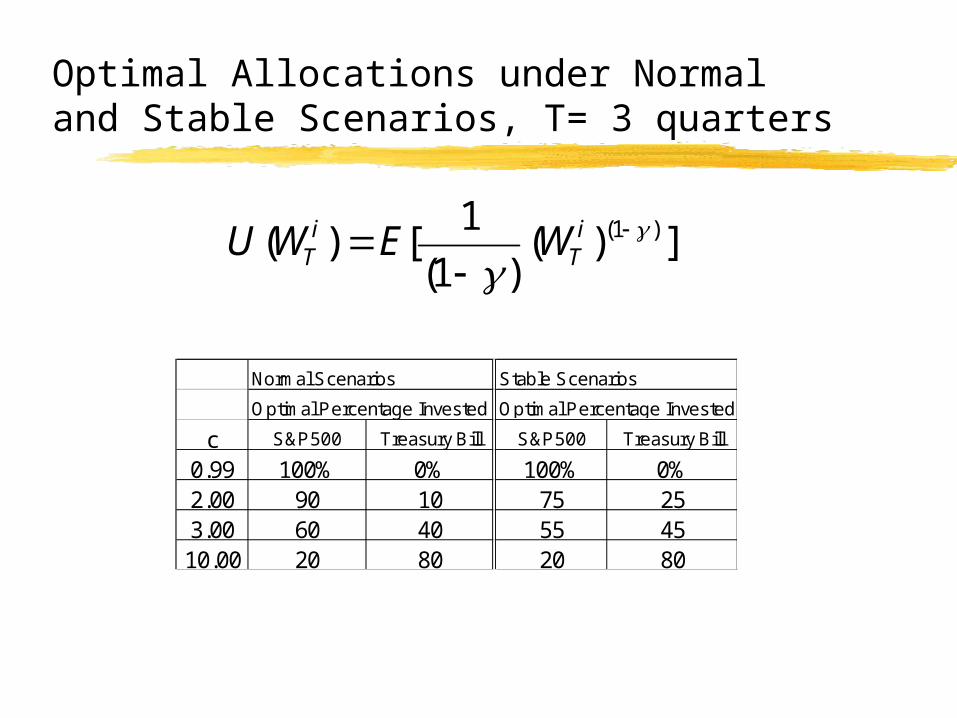
Optimal Allocations under Normal and Stable Scenarios, T= 3 quarters

Normal Scenarios Stable Scenarios

Optimal Percentage Invested Optimal Percentage Invested

c S&P500 Treasury Bill S&P500 Treasury Bill

0.99 100% 0% 100% 0%2.00 90 10 75 253.00 60 40 55 4510.00 20 80 20 80

])()1(

1[)( )1(

i

TiT WEWU

VII. Conclusion

Optimal asset allocation may be sensitive to the distributional assumption

We need to model heavy tails more realistically

Future work: stochastic programming without decision rules