Nonlinear Dyn

DOI 10.1007/s11071-007-9244-z

O R I G I N A L A R T I C L E

Stability properties of equilibrium sets of non-linearmechanical systems with dry friction and impactR. I. Leine · N. van de Wouw

Received: 24 May 2005 / Accepted: 4 January 2007C© Springer Science + Business Media B.V. 2007

Abstract In this paper, we will give conditions under

which the equilibrium set of multi-degree-of-freedom

non-linear mechanical systems with an arbitrary num-

ber of frictional unilateral constraints is attractive. The

theorems for attractivity are proved by using the frame-

work of measure differential inclusions together with

a Lyapunov-type stability analysis and a generalisation

of LaSalle’s invariance principle for non-smooth sys-

tems. The special structure of mechanical multi-body

systems allows for a natural Lyapunov function and an

elegant derivation of the proof. Moreover, an instabil-

ity theorem for assessing the instability of equilibrium

sets of non-linear mechanical systems with frictional

bilateral constraints is formulated. These results are il-

lustrated by means of examples with both unilateral

and bilateral frictional constraints.

Keywords Attractivity · Lyapunov stability ·Measure differential inclusion · Unilateral constraint

R. I. Leine (�)IMES – Center of Mechanics, ETH Zurich, CH-8092Zurich, Switzerlande-mail: remco.leine@imes.mavt.ethz.ch

N. van de WouwDepartment of Mechanical Engineering, EindhovenUniversity of Technology, P.O. Box 513, 5600 MBEindhoven, The Netherlandse-mail: N.v.d.Wouw@tue.nl

1 Introduction

Dry friction can seriously affect the performance of

a wide range of systems. More specifically, the stic-

tion phenomenon in friction can induce the presence

of equilibrium sets, see for example [46]. The stability

properties of such equilibrium sets is of major interest

when analysing the global dynamic behaviour of these

systems.

The aim of the paper is to present a number of the-

oretical results that can be used to rigourously prove

the conditional attractivity of the equilibrium set for

non-linear mechanical systems with frictional unilat-

eral constraints (including impact) using Lyapunov sta-

bility theory and LaSalle’s invariance principle.

The dynamics of mechanical systems with set-

valued friction laws are described by differential in-

clusions of Filippov-type (so-called Filippov systems),

see [27, 31] and references therein. Filippov systems,

describing systems with friction, can exhibit equilib-

rium sets, which correspond to the stiction behaviour

of those systems. Many publications deal with stabil-

ity and attractivity properties of (sets of) equilibria in

differential inclusions [1–3, 6, 21, 26, 43, 47]. For ex-

ample, in [2, 43] the attractivity of the equilibrium set of

a dissipative one-degree-of-freedom friction oscillator

with one switching boundary (i.e. one dry friction ele-

ment) is discussed. Moreover, in [3, 6, 43] the Lyapunov

stability of an equilibrium point in the equilibrium set

is shown. Most papers are limited to either one-degree-

of-freedom systems or to systems exhibiting only one

Springer

Nonlinear Dyn

switching boundary. Very often, the stability proper-

ties of an equilibrium point in the equilibrium set is

investigated and not the stability properties of the set

itself. In this context, it is worth mentioning that in the

more general scope of discontinuous systems (with-

out impulsive loads), a range of results regarding sta-

bility conditions for isolated equilibria are available,

see for example [23] in which conditions for stabil-

ity are formulated in terms of the existence of com-

mon quadratic or piece-wise quadratic Lyapunov func-

tions. Yakubovich et al. [47] discuss the stability and

dichotomy (a form of attractivity) of equilibrium sets in

differential inclusions within the framework of absolute

stability. In [9], extensions are given of the absolute sta-

bility problem and the Lagrange–Dirichlet theorem for

systems with monotone multi-valued mappings (such

as, for example Coulomb friction and unilateral contact

constraints). In the absolute stability framework, strict

passivity properties of a linear part of the system are

required for proving the asymptotic stability of an iso-

lated equilibrium point, which may be rather restrictive

for mechanical systems in general. Adly et al. [1, 21]

study stability properties of equilibrium sets of differ-

ential inclusions describing mechanical systems with

friction. It is assumed that the non-smoothness is stem-

ming from a maximal monotone operator (e.g. friction

with a constant normal force). Existence and unique-

ness of solutions is therefore always fulfilled. A basic

Lyapunov theorem for stability and attractivity is given

in [1, 21] for first-order differential inclusions with

maximal monotone operators. The results are applied to

linear mechanical systems with friction. It is assumed

in [1] that the relative sliding velocity of the frictional

contacts depends linearly on the generalised velocities.

Conditions for the attractivity of an equilibrium set are

given. The results are generalised in [1] to conserva-

tive systems with an arbitrary potential energy function.

In a previous publication [45], we provided conditions

under which the equilibrium set of multi-degree-of-

freedom linear mechanical systems with an arbitrary

number of Coulomb friction elements is attractive using

Lyapunov-type stability analysis and a generalisation

of LaSalle’s invariance principle for non-smooth sys-

tems. Moreover, dissipative as well as non-dissipative

linear systems have been considered. The analysis was

restricted to bilateral frictional constraints and linear

systems.

Unilateral contact between rigid bodies does not

only lead to the possible separation of contacting bod-

ies but can also lead to impact when bodies collide.

Systems with impact between rigid bodies undergo in-

stantaneous changes in the velocities of the bodies.

Impact systems, with or without friction, can be prop-

erly described by measure differential inclusions as in-

troduced by Moreau [32, 34] (see also [8, 18, 31]),

which allow for discontinuities in the state of the sys-

tem. Measure differential inclusions, being more gen-

eral than Filippov systems, can exhibit equilibrium sets

as well. The results in [9] on the absolute stability prob-

lem and the Lagrange–Dirichlet theorem apply also to

systems with unilateral contact and impact. However,

once more only the stability of isolated equilibria is ad-

dressed. In [12], stability conditions of isolated equi-

libria for a class of discontinuous systems (with state-

jumps), formulated as cone-complementarity systems,

are posed using a passivity-based approach.

The stability of hybrid systems with state-

discontinuities is addressed by a vast number of re-

searchers in the field of control theory. The book of

Bainov and Simeonov [7] focuses on systems with

impulsive effects and gives many useful Russian ref-

erences. Lyapunov stability theorems, instability theo-

rems and theorems for boundedness are given by Ye

et al. [48]. Pettersson and Lennartson [38] propose

stability theorems using multiple Lyapunov functions.

By using piecewise quadratic Lyapunov function can-

didates and replacing the regions where the different

stability conditions have to be valid by quadratic in-

equality functions (and exploiting the S-procedure), the

problem of verifying stability is turned into a Linear

Matrix Inequality (LMI) problem. See also the review

article of Davrazos and Koussoulas [15]. Many publi-

cations focus on the control of mechanical systems with

frictionless unilateral contacts by means of Lyapunov

functions. See, for instance Brogliato et al. [11] and

Tornambe [44] and the book [8] for further references.

The Lagrange–Dirichlet stability theorem is ex-

tended by Brogliato [9] to measure differential

inclusions describing mechanical systems with fric-

tionless impact. The idea to use Lyapunov functions

involving indicator functions associated with unilateral

constraints is most probably due to [9]. More gener-

ally, the work of Chareyron and Wieber [13, 14] is

concerned with a Lyapunov stability framework for

measure differential inclusions describing mechani-

cal systems with frictionless impact. It is clearly ex-

plained in [14] why the Lyapunov function has to be

globally positive definite, in order to prove stability in

Springer

Nonlinear Dyn

the presence of state-discontinuities (when no further

assumptions on the system or the form of the Lyapunov

function are made). The importance of this condition

has also been stated in [7, 48] for hybrid systems and

in [11, 44] for mechanical systems with frictionless

unilateral constraints. Moreover, LaSalle’s invariance

principle is generalised in [10] to differential inclusions

and in [13, 14] to measure differential inclusions de-

scribing mechanical systems with frictionless impact.

The proof of LaSalle’s invariance principle strongly re-

lies on the positive invariance of limit sets. It is assumed

in [13, 14] that the system enjoys continuity of the so-

lution with respect to the initial condition which is a

sufficient condition for positive invariance of limit sets.

In [14], an extension of LaSalle invariance principle to

systems with unilateral constraints is presented (more

specifically, it is applied to mechanical systems with

frictionless unilateral contacts). In [10], an extension

of LaSalle invariance principle for a class of unilateral

dynamical systems, the so-called evolution variational

inequalities, is presented.

Instability results for finite-dimensional variational

inequalities can be found in the work of Goeleven and

Brogliato [20, 21], whereas Quittner [40] gives insta-

bility results for a class of parabolic variational inequal-

ities in Hilbert spaces.

In this paper, we will give conditions under which the

equilibrium set of multi-degree-of-freedom non-linearmechanical systems with an arbitrary number of fric-

tional unilateral constraints (i.e. systems with friction

and impact) is attractive. The theorems for attractivity

are proved by using the framework of measure differen-

tial inclusions together with a Lyapunov-type stability

analysis and a generalisation of LaSalle’s invariance

principle for non-smooth systems, which is based on

the assumption that every limit set is positively invari-

ant (see also [28]). The special structure of mechanical

multi-body systems allows for a natural choice of the

Lyapunov function and a systematic derivation of the

proof for this large class of systems.

In Sections 2 and 3, the constitutive laws for fric-

tional unilateral contact and impact are formulated as

set-valued force laws. The modelling of mechanical

systems with dry friction and impact by measure dif-

ferential inclusions is discussed in Section 4. Subse-

quently, the attractivity properties of the equilibrium set

of a system with frictional unilateral contact are studied

in Section 5. Non-linear mechanical systems with bilat-

eral frictional constraints form an important sub-class

of systems and are studied in Section 6, where also in-

stability conditions for equilibrium sets are proposed.

Moreover, for both classes of systems the attractivity

analysis provides an estimate for the region of attrac-

tion of the equilibrium sets. In Section 7, a number of

examples are studied in order to illustrate the theoreti-

cal results of Sections 5 and 6. Moreover, an example is

given that shows the conservativeness of the estimated

region of attraction. Finally, a discussion of the results

and concluding remarks are given in Section 8.

2 Frictional contact laws in the form of set-valuedforce laws

In this section, we formulate the constitutive laws for

frictional unilateral contact formulated as set-valued

force laws (see [18] for an extensive treatise on the

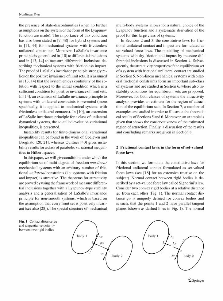
subject). Normal contact between rigid bodies is de-

scribed by a set-valued force law called Signorini’s law.

Consider two convex rigid bodies at a relative distance

gN from each other (Fig. 1). The normal contact dis-

tance gN is uniquely defined for convex bodies and

is such, that the points 1 and 2 have parallel tangent

planes (shown as dashed lines in Fig. 1). The normal

Fig. 1 Contact distance gN

and tangential velocity γT

between two rigid bodies

Springer

Nonlinear Dyn

contact distance gN is non-negative because the bod-

ies do not penetrate into each other. The bodies touch

when gN = 0. The normal contact force λN between

the bodies is non-negative because the bodies can exert

only repelling forces on each other, i.e. the constraint

is unilateral. The normal contact force vanishes when

there is no contact, i.e. gN > 0, and can only be positive

when contact is present, i.e. gN = 0. Under the assump-

tion of impenetrability, expressed by gN ≥ 0, only two

situations may occur:

gN = 0 ∧ λN ≥ 0 contact,

gN > 0 ∧ λN = 0 no contact.(1)

From Equation (1), we see that the normal contact law

shows a complementarity behaviour: the product of the

contact force and normal contact distance is always

zero, i.e. gNλN = 0. The relation between the normal

contact force and the normal contact distance is there-

fore described by

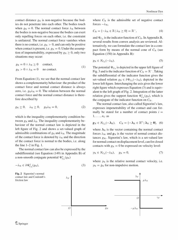
gN ≥ 0, λN ≥ 0, gNλN = 0, (2)

which is the inequality complementarity condition be-

tween gN and λN. The inequality complementarity be-

haviour of the normal contact law is depicted in the

left figure of Fig. 2 and shows a set-valued graph of

admissible combinations of gN and λN. The magnitude

of the contact force is denoted by λN and the direction

of the contact force is normal to the bodies, i.e. along

the line 1–2 in Fig. 1.

The normal contact law can also be expressed by the

subdifferential (see Equation (149) in Appendix B) of

a non-smooth conjugate potential �∗CN

(gN)

−λN ∈ ∂�∗CN

(gN), (3)

where CN is the admissible set of negative contact

forces −λN,

CN = {−λN ∈ R | λN ≥ 0} = R−, (4)

and �CNis the indicator function of CN. In Appendix B,

several results from convex analysis are reviewed. Al-

ternatively, we can formulate the contact law in a com-

pact form by means of the normal cone of CN (see

Equation (150) in Appendix B):

gN ∈ NCN(−λN). (5)

The potential �CNis depicted in the upper left figure of

Fig. 3 and is the indicator function of CN = R−. Taking

the subdifferential of the indicator function gives the

set-valued relation gN ∈ ∂�CN(−λN), depicted in the

lower left figure. Interchanging the axis gives the lower

right figure which expresses Equation (3) and is equiv-

alent to the left graph of Fig. 2. Integration of the latter

relation gives the support function �∗CN

(gN), which is

the conjugate of the indicator function on CN.

The normal contact law, also called Signorini’s law,

expresses impenetrability of the contact and can for-

mally be stated for a number of contact points i =1, . . . , nC as

gN ∈ NCN(−λN), CN = {−λN ∈ Rn |λN ≥ 0}, (6)

where λN is the vector containing the normal contact

forces λNi and gN is the vector of normal contact dis-

tances gNi . Signorini’s law, which is a set-valued law

for normal contact on displacement level, can for closed

contacts with gN = 0 be expressed on velocity level:

γN ∈ NCN(−λN), gN = 0, (7)

where γN is the relative normal contact velocity, i.e.

γN = gN for non-impulsive motion.

Fig. 2 Signorini’s normalcontact law and Coulomb’sfriction law

Springer

Nonlinear Dyn

Fig. 3 Potential, conjugatepotential and subdifferentialof the normal contactproblem C = CN = R−

Coulomb’s friction law is another classical example

of a force law that can be described by a non-smooth

potential. Consider two bodies as depicted in Fig. 1 with

Coulomb friction at the contact point. We denote the

relative velocity of point 1 with respect to point 2 along

their tangent plane by γT. If contact is present between

the bodies, i.e. gN = 0, then the friction between the

bodies imposes a force λT along the tangent plane of

the contact point. If the bodies are sliding over each

other, then the friction force λT has the magnitude μλN

and acts in the direction of −γT

−λT = μλN sign(γT), γT �= 0, (8)

where μ is the friction coefficient and λN is the nor-

mal contact force. If the relative tangential velocity

vanishes, i.e. γT = 0, then the bodies purely roll over

each other without slip. Pure rolling, or no slip for

locally flat objects, is denoted by stick. If the bodies

stick, then the friction force must lie in the interval

−μλN ≤ λT ≤ μλN. For unidirectional friction, i.e. for

planar contact problems, the following three cases are

possible:

γT = 0 ⇒ |λT| ≤ μλN sticking,

γT < 0 ⇒ λT = +μλN negative sliding,

γT > 0 ⇒ λT = −μλN positive sliding.

(9)

We can express the friction force by a potential πT(γT),

which we mechanically interpret as a dissipation func-

tion,

−λT ∈ ∂πT(γT), πT(γT) = μλN|γT|, (10)

from which follows the set-valued force law

−λT ∈

⎧⎪⎨⎪⎩μλN, γT > 0,

[−1, 1]μλN, γT = 0,

−μλN, γT < 0.

(11)

A non-smooth convex potential therefore leads to a

maximal monotone set-valued force law. The admis-

sible values of the negative tangential force λT form

a convex set CT that is bounded by the values of the

normal force [39]:

CT = {−λT | −μλN ≤ λT ≤ +μλN}. (12)

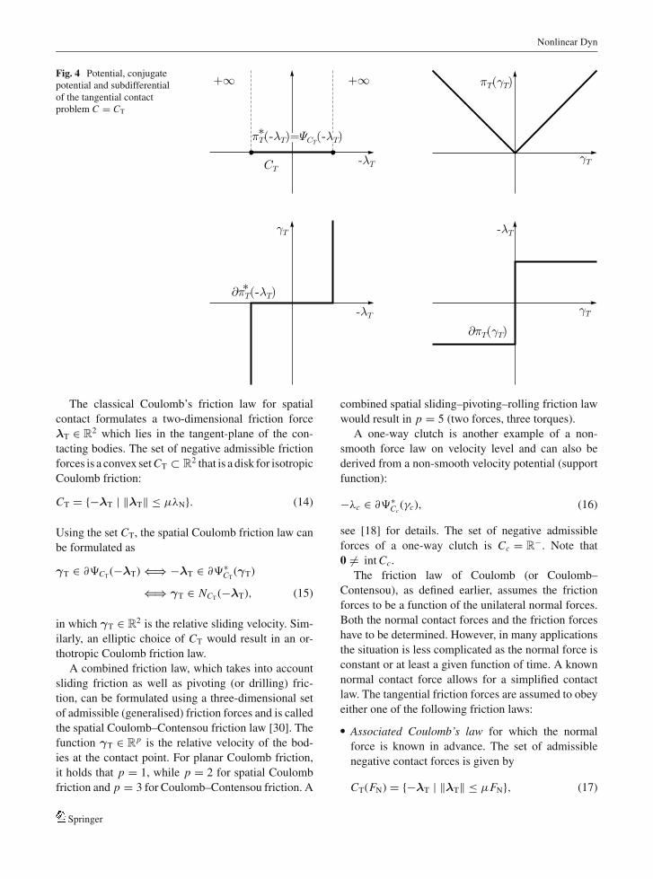
Coulomb’s law can be expressed with the aid of the

indicator function of CT as

γT ∈ ∂�CT(−λT) ⇔ γT ∈ NCT

(−λT), (13)

where the indicator function �CTis the conjugate po-

tential of the support function πT(γT) = �∗CT

(γT) [18],

see Fig. 4.

Springer

Nonlinear Dyn

Fig. 4 Potential, conjugatepotential and subdifferentialof the tangential contactproblem C = CT

The classical Coulomb’s friction law for spatial

contact formulates a two-dimensional friction force

λT ∈ R2 which lies in the tangent-plane of the con-

tacting bodies. The set of negative admissible friction

forces is a convex set CT ⊂ R2 that is a disk for isotropic

Coulomb friction:

CT = {−λT | ‖λT‖ ≤ μλN}. (14)

Using the set CT, the spatial Coulomb friction law can

be formulated as

γT ∈ ∂�CT(−λT) ⇐⇒ −λT ∈ ∂�∗

CT(γT)

⇐⇒ γT ∈ NCT(−λT), (15)

in which γT ∈ R2 is the relative sliding velocity. Sim-

ilarly, an elliptic choice of CT would result in an or-

thotropic Coulomb friction law.

A combined friction law, which takes into account

sliding friction as well as pivoting (or drilling) fric-

tion, can be formulated using a three-dimensional set

of admissible (generalised) friction forces and is called

the spatial Coulomb–Contensou friction law [30]. The

function γT ∈ Rp is the relative velocity of the bod-

ies at the contact point. For planar Coulomb friction,

it holds that p = 1, while p = 2 for spatial Coulomb

friction and p = 3 for Coulomb–Contensou friction. A

combined spatial sliding–pivoting–rolling friction law

would result in p = 5 (two forces, three torques).

A one-way clutch is another example of a non-

smooth force law on velocity level and can also be

derived from a non-smooth velocity potential (support

function):

−λc ∈ ∂�∗Cc

(γc), (16)

see [18] for details. The set of negative admissible

forces of a one-way clutch is Cc = R−. Note that

0 �= int Cc.

The friction law of Coulomb (or Coulomb–

Contensou), as defined earlier, assumes the friction

forces to be a function of the unilateral normal forces.

Both the normal contact forces and the friction forces

have to be determined. However, in many applications

the situation is less complicated as the normal force is

constant or at least a given function of time. A known

normal contact force allows for a simplified contact

law. The tangential friction forces are assumed to obey

either one of the following friction laws:� Associated Coulomb’s law for which the normal

force is known in advance. The set of admissible

negative contact forces is given by

CT(FN) = {−λT | ‖λT‖ ≤ μFN}, (17)

Springer

Nonlinear Dyn

which is dependent on the known normal forces FN

and friction coefficient μ. This friction law is de-

scribed by a maximal monotone set-valued operator

(the Sign-function in the planar case) on the relative

sliding velocity γT.� Non-associated Coulomb’s law for which the nor-

mal force is dependent on the generalised coordi-

nates q and/or generalised velocities u and therefore

not known in advance. The set of admissible negative

contact forces is given by

CT(λN) = {−λT | ‖λT‖ ≤ μλN}, (18)

which is dependent on the normal contact forces λN

and friction coefficient μ. Non-associated Coulomb

friction is not described by a maximal monotone op-

erator on γT, since the normal contact force λN varies

in time.

3 Impact laws

Signorini’s law and Coulomb’s friction law are set-

valued force laws for non-impulsive forces. In order

to describe impact, we need to introduce impact laws

for the contact impulses. We will consider a Newton-

type of restitution law,

γ +N = −eNγ −

N , gN = 0, (19)

which relates the post-impact velocity γ +N of a contact

point to the pre-impact velocity γ −N by Newton’s coef-

ficient of restitution eN. The case eN = 1 corresponds

to a completely elastic contact, whereas eN = 0 corre-

sponds to a completely inelastic contact. The impact,

which causes the sudden change in relative velocity,

is accompanied by a normal contact impulse �N > 0.

Following [17], suppose that, for any reason, the con-

tact does not participate in the impact, i.e. that the value

of the normal contact impulse �N is zero, although

the contact is closed. This happens normally for multi-

contact situations. For this case, we allow the post-

impact relative velocities to be higher than the value

prescribed by Newtons impact law, γ +N > −eNγ −

N , in

order to express that the contact is superfluous and

could be removed without changing the contact-impact

process. We can therefore express the impact law as an

inequality complementarity on velocity–impulse level:

�N ≥ 0, ξN ≥ 0, �NξN = 0, (20)

with ξN = γ +N + eNγ −

N (see [17]). Similarly to Sig-

norini’s law on velocity level, we can write the impact

law in normal direction as

ξN ∈ NCN(−�N), gN = 0, (21)

or by using the support function

−�N ∈ ∂�∗CN

(ξN), gN = 0. (22)

A normal contact impulse �N at a frictional con-

tact leads to a tangential contact impulse ΛT with

‖ΛT‖ ≤ μ�N. We therefore have to specify a tangen-

tial impact law as well. The tangential impact law can

be formulated in a similar way as has been done for the

normal impact law:

−ΛT ∈ ∂�∗CT(�N)(ξT), gN = 0, (23)

with ξT = γ+T + eTγ

−T . This impact law involves a tan-

gential restitution coefficient eT. This restitution coef-

ficient, which is normally considered to be zero, can

be used to model the tangential velocity reversal as ob-

served in the motion of the Super Ball, being a very

elastic ball used on play grounds. More information

on the physical meaning of the tangential restitution

coefficient can be found in [37].

4 Modelling of non-linear mechanical systemswith dry friction and impact

In this section, we will define the class of non-linear

time-autonomous mechanical systems with unilateral

frictional contact for which the stability results will be

derived in Section 5. We first derive a measure differ-

ential inclusion that describes the temporal dynamics

of mechanical systems with discontinuities in the ve-

locity. Subsequently, we study the equilibrium set of

the measure differential inclusion.

4.1 The measure differential inclusion

We assume that these mechanical systems exhibit only

bilateral holonomic frictionless constraints and unilat-

eral constraints in which dry friction can be present.

Furthermore, we assume that a set of independent gen-

eralised coordinates, q ∈ Rn , for which these bilateral

constraints are eliminated from the formulation of the

Springer

Nonlinear Dyn

dynamics of the system, is known. The generalised co-

ordinates q(t) are assumed to be absolutely continuous

functions of time t . Also, we assume the generalised

velocities, u(t) = q(t) for almost all t , to be functions

of locally bounded variation. At each time-instance it

is therefore possible to define a left limit u− and a right

limit u+ of the velocity. The generalised accelerations

u are therefore not for all t defined. The set of disconti-

nuity points {t j } for which u is not defined is assumed to

be Lebesgue negligible. We formulate the dynamics of

the system using a Lagrangian approach, resulting in1

(d

dt(T,u) − T,q + U,q

)T

= f nc(q, u) + WN(q)λN + WT(q)λT, (24)

or, alternatively,

M(q)u − h(q, u) = WN(q)λN + WT(q)λT, (25)

which is a differential equation for the non-impulsive

part of the motion. Herein, M(q) = MT(q) > 0 is

the mass-matrix. The scalar T represents kinetic

energy and it is assumed that it can be written as T =12uT M(q)u. Moreover, U denotes the potential energy.

The column-vector f nc in Equation (24) represents all

smooth generalised non-conservative forces. The state-

dependent column-vector h(q, u) in Equation (25)

contains all differentiable forces (both conservative and

non-conservative), such as spring forces, gravitation,

smooth damper forces and gyroscopic terms.

We introduce the following index sets:

IG = {1, . . . , nC} the set of all contacts,

IN = {i ∈ IG | gNi (q) = 0}the set of all closed contacts, (26)

and set up the force laws and impact laws of each con-

tact as has been elaborated in Sections 2 and 3. The

normal contact distances gNi (q) depend on the gener-

alised coordinates q and are gathered in a vector gN(q).

During a non-impulsive part of the motion, the

normal contact force −λNi ∈ CN and friction force

−λTi ∈ CTi ⊂ Rp of each closed contact i ∈ IN, are

1 Note that the sub-script ,x indicates a partial derivative opera-tion ∂/∂x .

assumed to be associated with a non-smooth potential,

being the support function of a convex set, i.e.

−λNi ∈ ∂�∗CN

(γNi ), −λTi ∈ ∂�∗CTi

(γTi ), (27)

where CN = R− and the set CTi can be dependent on

the normal contact force λNi ≥ 0. The normal and tan-

gential contact forces of all nC contacts are gathered

in columns λN = {λNi } and λT = {λTi } and the corre-

sponding normal and tangential relative velocities are

gathered in columns γN = {γNi } and γT = {γTi }, for

i ∈ IG . We assume that these contact velocities are re-

lated to the generalised velocities through:

γN(q, u) = WTN(q)u, γT(q, u) = WT

T(q)u. (28)

It should be noted that WTX (q) = ∂γX

∂u for X = N , T .

This assumption is very important as it excludes rheo-

nomic contacts.

Equation (25) together with the set-valued force

laws (27) form a differential inclusion

M(q)u − h(q, u) ∈ −∑i∈IN

WNi (q)∂�∗CN

(γNi )

− WTi (q)∂�∗CTi

(γTi ), for almost all t. (29)

Differential inclusions of this type are called Filippov

systems [16]. The differential inclusion (29) only holds

for impact free motion.

Subsequently, we define for each contact point the

constitutive impact laws

−�Ni ∈ ∂�∗CN

(ξNi ), −ΛTi ∈ ∂�∗CTi (�Ni )

(ξTi ),

i ∈ IN, (30)

with

ξNi = γ +Ni + eNiγ

−Ni , ξTi = γ+

Ti + eTiγ−Ti , (31)

in which eNi and eTi are the normal and tangential resti-

tution coefficients, respectively. The inclusions (30)

form very complex set-valued mappings representing

the contact laws at the impulse level. The force laws for

non-impulsive motion can be put in the same form be-

cause u+ = u− holds in the absence of impacts and

because of the positive homogeneity of the support

function (see Appendix B):

−λNi ∈ ∂�∗CN

(ξNi ), −λTi ∈ ∂�∗CTi (λNi )

(ξTi ). (32)

Springer

Nonlinear Dyn

We now replace the differential inclusion (29), which

holds for almost all t , by an equality of measures

M(q) du − h(q, u) dt

= WN(q) dΛN + WT(q) dΛT ∀t, (33)

which holds for all time-instances t . The differential

measure of the contact impulsions dΛN and dΛT con-

tains a Lebesgue measurable part λ dt and an atomic

part Λ dη

dΛN = λN dt + ΛN dη, dΛT = λT dt + ΛT dη,

(34)

which can be expressed as inclusions

−d�Ni ∈ ∂�∗CN

(ξNi )(dt + dη),

−dΛTi ∈ ∂�∗CTi (λNi )

(ξTi ) dt + ∂�∗CTi (�Ni )

(ξTi ) dη.

(35)

As an abbreviation we write

M(q) du − h(q, u) dt = W(q) dΛ ∀t, (36)

using short-hand notation

λ =[λN

λT

], Λ =

[ΛN

ΛT

],

W = [ WN WT ], γ =[γN

γT

]. (37)

Furthermore we introduce the quantities

ξ ≡ γ+ + Eγ−, δ ≡ γ+ − γ−, (38)

with E = diag({eNi , eTi }) from which we deduce

γ+ = (I + E)−1(ξ + Eδ),

γ− = (I + E)−1(ξ − δ).(39)

The equality of measures (36) together with the set-

valued force laws (35) form a measure differential

inclusion that describes the time-evolution of a me-

chanical system with discontinuities in the generalised

velocities. Such a measure differential inclusion does

not necessarily have existence and uniqueness of solu-

tions for all admissible initial conditions. Indeed, if the

friction coefficient is large, then the coupling between

motion normal to the constraint and tangential to the

constraint can cause existence and uniqueness prob-

lems (known as the Painleve problem [8, 29]). In the

following, we will assume existence and uniqueness of

solutions in forward time. The contact laws guarantee

that the generalised positions q(t) are such that penetra-

tion is avoided (gNi ≥ 0) and the generalised positions

therefore remain within the admissible set

K = {q ∈ Rn | gNi (q) ≥ 0 ∀i ∈ IG}, (40)

for all t . The condition q(t) ∈ K follows of course from

the assumption of existence of solutions. We remark,

however, that the following theorems can be relaxed to

systems with non-uniqueness of solutions.

4.2 Equilibrium set

The measure differential inclusion described by

Equations (36) and (35) exhibits an equilibrium set.

Note that the assumption of scleronomic contacts im-

plies that γT = 0 for u = 0, see Equation (28). This

means that every equilibrium implies sticking in all

closed contact points. Every equilibrium position has

to obey the equilibrium inclusion

h(q, 0)−∑i∈IN

(WNi (q)∂�∗

CN(0) + WTi (q)∂�∗

CTi(0)

)�0,

(41)

which, using C = ∂�∗C (0), simplifies to

h(q, 0) −∑i∈IN

(WNi (q)CNi + WTi (q)CTi ) � 0. (42)

An equilibrium set, being a simply connected set of

equilibrium points, is therefore given by (CNi = −R+)

E ⊂{

(q, u) ∈ Rn × Rn| (u = 0) ∧ h(q, 0)

+∑i∈IN

(WNi (q)R+ − WTi (q)CTi ) � 0

}(43)

and is positively invariant if we assume uniqueness of

the solutions in forward time. WithE we denote an equi-

librium set of the measure differential inclusion in the

state-space (q, u), while Eq is reserved for the union of

Springer

Nonlinear Dyn

equilibrium positions q∗, i.e. E = {(q, u) ∈ Rn × Rn |q ∈ Eq , u = 0}. Note that non-linear mechanical sys-

tems without dry friction can exhibit multiple equilib-

ria. Similarly, a system with dry friction may exhibit

multiple equilibrium sets.

Let us now state some consequences of the assump-

tions made, which will be used in the next section. Due

to the fact that the kinetic energy can be described by

T = 1

2uT M(q)u = 1

2

∑r

∑s

Mrsur us, (44)

with M(q) = MT(q), we can write in tensorial

language

∂T

∂qk= 1

2

∑r

∑s

(∂ Mrs

∂qk

)ur us,

∂T

∂uk=

∑r

Mkr ur ,

d

dt

(∂T

∂uk

)=

∑r

Mkr ur +∑

r

∑s

(∂ Mkr

∂qs

)ur us

=∑

r

Mkr ur + 2∂T

∂qk

+∑

r

∑s

(∂ Mkr

∂qs− ∂ Mrs

∂qk

)ur us

d

dt(T,u) = uT M(q) + 2T,q − ( f gyr)T

for almost all t (45)

with the gyroscopic forces [36]

f gyr = {f gyrk

},

f gyrk = −

∑r

∑s

(∂ Mkr

∂qs− ∂ Mrs

∂qk

)ur us . (46)

In the next section, we will exploit that the gyroscopic

forces f gyr have zero power [36]

uT f gyr =∑

k

uk f gyrk

= −∑

k

∑r

∑s

(∂ Mkr

∂qs− ∂ Mrs

∂qk

)ur usuk = 0.

(47)

In the same way as before, we can write the differential

measure of T,u as

d(T,u) = duT M(q) + 2T,q dt − ( f gyr)T dt ∀t. (48)

Comparison with Equations (25) and (24) yields

h = f nc + f gyr − (T,q + U,q )T, (49)

or in index notation

hk = f nck − ∂U

∂qk− ∂T

∂qk+ f gyr

k

= f nck − ∂U

∂qk− ∂T

∂qk−

∑r

∑s

(∂ Mkr

∂qs− ∂ Mrs

∂qk

)ur us

= f nck − ∂U

∂qk− 1

2

∑r

∑s

(2∂ Mkr

∂qs− ∂ Mrs

∂qk

)ur us

= f nck − ∂U

∂qk− 1

2

∑r

∑s

(∂ Mkr

∂qs+ ∂ Mks

∂qr− ∂ Mrs

∂qk

)ur us

= f nck − ∂U

∂qk−

∑r

∑s

k,rsur us (50)

in which we recognise the holonomic Christoffel sym-

bols of the first kind [36]

k,rs = k,sr := 1

2

(∂ Mkr

∂qs+ ∂ Mks

∂qr− ∂ Mrs

∂qk

). (51)

5 Attractivity of equilibrium sets for non-linearsystems

In this section, we will investigate the attractivity prop-

erties of the equilibrium sets defined in the previous

section.

We define the following non-linear functionals

Rn → R on u ∈ Rn:� Dncq (u) := −uT f nc(q, u) is the dissipation rate func-

tion of the smooth non-conservative forces.� DλTq (u) := ∑

i∈IN

11+eTi

�∗CTi (λNi )

(ξTi (q, u)) is the dis-

sipation rate function of the tangential contact forces.� D�Tq (u) := ∑

i∈IN

11+eTi

�∗CTi (�Ni )

(ξTi (q, u)) is the

dissipation rate function of the tangential contact

impulses.

Springer

Nonlinear Dyn

For non-impulsive motion it holds that γT = γ+T = γ−

T

and ξT = (1 + eT)γT. Due to the fact that the support

function is positively homogeneous, it follows that

DλTq (u) =

∑i∈IN

�∗CTi (λNi )

(γTi (q, u))

=∑i∈IN

−λTiγTi (q, u), (52)

from which we see that the dissipation rate function

of the tangential contact forces does not depend on the

restitution coefficient eT. The above dissipation rate

functions are of course functions of (q, u), but we write

them as non-linear functionals on u for every fixed qso that we can speak of the zero set of the functional

Dq (u):

D−1q (0) = {u ∈ Rn | Dq (u) = 0}. (53)

As stated before, the type of systems under investi-

gation may exhibit multiple equilibrium sets. Here, we

will study the attractivity properties of a specific given

equilibrium set. By qe we denote an equilibrium posi-

tion of the system with unilateral frictionless contacts

M(q)u − h(q, u) − W N (q)λN = 0, (54)

from which follows that the equilibrium position qe is

determined by the inclusion

h(qe, 0) −∑i∈IG

WNi (qe)∂�∗CN

(gNi (qe)) � 0 (55)

or

h(qe, 0) −∑i∈IN

WNi (qe)∂�∗CN

(γNi (qe, 0)︸ ︷︷ ︸=0

) � 0, (56)

which is equivalent to

h(qe, 0) + W N (qe)R+ � 0, W N = {WNi }, i ∈ IN.

(57)

Let the potential Q(q) be the total potential energy of

the system

Q(q) = U (q) +∑i∈IG

�∗CN

(gNi (q)), (58)

which is the sum of the potential energy of all smooth

potential forces and the support functions of the normal

contact forces. Moreover, we assume that the equilib-

rium position qe is a local minimum of the total poten-

tial energy Q(q), i.e.

Q(q) ={

0 q = qe

> 0 ∀q ∈ U\{qe}, 0 /∈ ∂ Q(q), ∀q ∈ U\{qe}.

(59)

The sub-set U is assumed to enclose the equilibrium

set Eq under investigation. Notice that the equilibrium

point qe of the system without friction is also an equi-

librium point of the system with friction, (qe, 0) ∈ E .

In case the system does exhibit multiple equilibrium

sets, the attractivity of E will be only local for obvi-

ous reasons. In the following, we will make use of the

Lyapunov candidate function

V = T (q, u) + Q(q)

= T (q, u) + U (q) +∑i∈IG

�∗CN

(gNi (q)), (60)

being the sum of kinetic and total potential energy.

The function V : Rn × Rn → R ∪ {∞} is an extended

lower semi-continuous function. Moreover, the func-

tion V (t) = V (q(t), u(t)) is of locally bounded varia-

tion in time (see Appendix D) because q(t) is absolutely

continuous and remains in the admissible set K defined

in (40), u ∈ lbv(I, Rn), and T is a Lipschitz continuous

function and Q is an extended lower semi-continuous

function but only dependent on q(t). In the following,

we will make use of the differential measure dV of

V (t). If it holds that dV ≤ 0, then it follows that

V +(t) − V −(t0) =∫

[t0,t]dV ≤ 0, (61)

which means that V (t) is non-increasing. Similarly,

dV < 0 implies a strict decrease of V (t). We now for-

mulate a technical result that states conditions under

which the equilibrium set can be shown to be (locally)

attractive.

Theorem 1 (Attractivity of the equilibrium set).Consider an equilibrium set E of the system (36), withconstitutive laws (27) and (35). If

1. T = 12uT M(q)u, with M(q) = MT(q) > 0,

Springer

Nonlinear Dyn

2. the equilibrium position qe is a local minimum ofthe total potential energy Q(q) and Q(q) has a non-vanishing generalised gradient for all q ∈ U\{qe},i.e. 0 /∈ ∂ Q(q) ∀q ∈ U\{qe}, and the equilibrium setEq is contained in U , i.e. Eq ⊂ U ,

3. Dncq (u) = −uT f nc ≥ 0, i.e. the smooth non-

conservative forces are dissipative, and f nc = 0for u = 0,

4. there exists a non-empty set IC ⊂ IG and an openneighbourhoodV ⊂ Rn × Rn of the equilibrium set,such that γNi (q, u) < 0 (a.e.) for ∀i ∈ IC\IN and(q, u) ∈ V ,

5. Dncq

−1(0) ∩ DλT Cq

−1(0) ∩ ker WT

NC (q) = {0}∀q ∈ Cwith

gNC = {gNi }, W NC = {wNi }for i ∈ IC as defined in 4.,

C = {q | gNC (q) = 0},DλT C

q =∑

i∈IC ∩IN

�∗CTi (λNi )

(γTi (q, u)),

6. 0 ≤ eNi < 1, |eTi | < 1 ∀i ∈ IG,7. one of the following conditions holds

a. the restitution coefficients are small in the sensethat 2emax

1+emax< 1

cond(G(q))∀q ∈ C where G(q) :=

W(q)T M(q)−1W(q) and emax is the largest resti-tution coefficient, i.e. emax ≥ max(eNi , eTi ) ∀i ∈IG,

b. all restitution coefficients are equal, i.e. e =eNi = eTi∀i ∈ IG,

c. friction is absent, i.e. μi = 0 ∀i ∈ IG,

8. E ⊂ Iρ∗ in which the set Iρ∗ , with Iρ = {(q, u) ∈Rn × Rn | V (q, u) < ρ}, is the largest level set ofV , given by (60), that is contained in V and Q ={(q, u) ∈ Rn × Rn | q ∈ U}, i.e.

ρ∗ = max{ρ:Iρ⊂(V∩Q)}

ρ, (62)

9. each limit set in Iρ∗ is positively invariant,

then the equilibrium set E is locally attractive and Iρ∗

is a conservative estimate for the region of attraction.

Proof: Note that V is positive definite around the equi-

librium point (q, u) = (qe, 0) due to conditions 1 and 2

in the theorem. Classically, we seek the time-derivative

of V in order to prove the decrease of V along solu-

tions of the system. However, u is not defined for all

t and u can undergo jumps. We therefore compute the

differential measure of V :

dV = dT + dQ. (63)

The total potential energy, being an extended lower

semi-continuous function, is only a function of the gen-

eralised displacements q, which are absolutely contin-

uous in time, and it therefore holds that

dQ = dQ(q)(dq)

= U,q dq + d�K(q)(dq), (64)

where d Q(q)(dq) is the subderivative (see Appendix C)

of Q at q in the direction dq = u dt . The subderivative

d�K(q)(dq) of the indicator function �K(q) equals the

indicator function on the associated contingent cone

KK(q) (see Equation (164))

d�K(q)(dq) = �KK(q)(dq). (65)

It holds that dq = u dt with u ∈ KK(q) due to the con-

sistency of the system and the indicator function on the

contingent cone therefore vanishes, i.e. �KK(q)(u dt) =0. Consequently, the differential measure of Q simpli-

fies to

dQ = U,q dq + �KK(q)(dq)

= U,qu dt + �KK(q)(u dt), u ∈ KK(q)

= U,qu dt.

(66)

The kinetic energy T (q, u) = 12uT M(q)u is a symme-

tric quadratic form in u. Using the results of

Appendix E, we deduce that the differential measure

of T is

dT = 1

2(u+ + u−)T M(q) du + T,q dq. (67)

The differential measure of the Lyapunov candidate Vbecomes

dV(66)+(67)= 1

2(u+ + u−)T M(q) du+(T,q + U,q ) dq

(36)= 1

2(u+ + u−)T (h(q, u) dt + W dΛ)

+ (T,q + U,q )u dt. (68)

Springer

Nonlinear Dyn

A term 12(u+ + u−)T dt in front of a Lebesgue measur-

able term equals uT dt . Together with Equation (49),

i.e. h = f nc + f gyr − (T,q + U,q )T, and Equation (34)

with Equation (37) we obtain

dV = uT f nc dt + uT f gyr dt + uTWλ dt

+ 1

2(u+ + u−)TWΛ dη. (69)

The gyroscopic forces have zero power uT f gyr = 0 (see

Equation (47)). Moreover, the constraints are assumed

to be scleronomic and according to Equation (28) it

therefore holds that γ = WTu, which gives

dV = uT f nc dt + γTλ dt + 1

2(γ+ + γ−)TΛ dη

(39)= uT f nc dt + γTλ dt + 12((I + E)−1(2ξ

− (I − E)δ))TΛ dη

= uT f nc dt + γTλ dt + ξT(I + E)−1Λ dη

− 1

2δT(I − E)(I + E)−1Λ dη

(34)+(38)= uT f nc dt + ξT(I + E)−1 dΛ

−1

2δT(I − E)(I + E)−1Λ dη

= uT f nc dt +∑i∈IN

(ξNi d�Ni

1 + eNi+ ξT

Ti dΛTi

1 + eTi

)−1

2δT(I − E)(I + E)−1Λ dη.

(70)

Using Equations (35) and (158), we obtain

ξNi d�Ni = −�∗CN

(ξNi )(dt + dη) = 0

ξTTi dΛTi = −�∗

CTi (λNi )(ξTi ) dt

−�∗CTi (�Ni )

(ξTi ) dη ≤ 0,

(71)

because of Equation (159) and�∗CN

(ξNi ) = �R+ (ξNi ) =0 for admissible ξNi ≥ 0. Moreover, applying

Equation (28) to Equation (38) gives

δ :=γ+ − γ− =WT(u+−u−)=WT M−1WΛ=GΛ,

(72)

in which we used the abbreviation

G := WT M−1W, (73)

which is known as the Delassus matrix [34]. The matrix

G is positive definite when W has full rank, because

M > 0. The matrix G is only positive semi-definite

if the matrix W does not have full rank, meaning

that the generalised force directions of the contact

forces are linearly dependent. However, we assume that

the matrix W only contains the generalised force di-

rections of unilateral constraints, and that these uni-

lateral constraints do not constitute a bilateral con-

straint. It therefore holds that there exists no ΛN �= 0such that WNΛN = 0. The impact law requires that

ΛN ≥ 0. Hence, it holds that ΛTNWT

N M−1WNΛN > 0

for all ΛN �= 0 with ΛN ≥ 0, even if the unilateral

constraints are linearly dependent. Moreover, ΛT �= 0implies ΛN �= 0. The inequality ΛTGΛ > 0 there-

fore holds for all Λ �= 0 which obey the impact

law (22), even if dependent unilateral constraints are

considered.

Using Equation (72), we can put the last term in

Equation (70) in the following quadratic form

1

2δT(I − E)(I + E)−1Λ dη

= 1

2ΛTG(I − E)(I + E)−1Λ dη. (74)

in which G(I − E)(I + E)−1 is a square matrix.

The matrix (I − E)(I + E)−1 is a diagonal matrix

which is positive definite if the contacts are not purely

elastic, i.e. 0 ≤ eNi < 1 and 0 ≤ eTi < 1 for all i . The

smallest diagonal element of (I − E)(I + E)−1 is1−emax

1+emax. Using Proposition 4 in Appendix A, we deduce

that if G is positive definite and if condition 7a holds,

then the positive definiteness of G(I − E)(I + E)−1

implies

1

2ΛTG(I − E)(I + E)−1Λ > 0, ∀Λ �= 0. (75)

If the generalised force directions are linearly de-

pendent, then the Delassus matrix G is singular and

cond(G) is infinity. Condition 7a can therefore not hold.

If G is positive semi-definite (or even positive defi-

nite) and all restitution coefficients are equal to e (con-

dition 7b), then the product 12ΛTG(I − E)(I + E)−1Λ

simplifies to 12

1−e1+eΛ

TGΛ which is in general non-

negative. Again, we can show that Equation (75) still

holds for dependent unilateral constraints if we con-

sider Λ �= 0 with Λ ≥ 0.

If G is positive semi-definite (or even positive def-

inite) and friction is absent (condition 7c: μi = 0∀i ∈

Springer

Nonlinear Dyn

IG ), then it holds that

1

2ΛTG(I − E)(I + E)−1Λ

= 1

2(γ+

N − γ−N)T(I − E)(I + E)−1ΛN

=∑

i

1

2(γ +

Ni − γ −Ni )

1 − eNi

1 + eNi�Ni . (76)

The impact law requires that γ +Ni + eNiγ

−Ni > 0 and

�Ni ≥ 0. Moreover, the unilateral contacts did not pen-

etrate before the impact and the pre-impact relative ve-

locities γ −Ni are therefore non-positive. The post-impact

relative velocities γ +Ni = −eNiγ

−Ni are therefore non-

negative for 0 ≤ eNi < 1. Furthermore, if �Ni > 0,

then it must hold that γ −Ni < 0. Hence, 1

2ΛTG(I −

E)(I + E)−1Λ > 0 for all Λ �= 0 with Λ ≥ 0.

Looking again at the differential measure of the total

energy (70), we realise that (under conditions 6 and 7)

all terms related to the contact forces and impulses are

dissipative or passive. Moreover, if we consider not

purely elastic contacts, then nonzero contact impulses

Λ strictly dissipate energy.

We can now decompose the differential measure dVin a Lebesgue part and an atomic part

dV = V dt + (V + − V −) dη, (77)

with (see Equation (52) and above)

V = uT f nc −∑i∈IN

1

1 + eTi�∗

CTi (λNi )(ξTi )

= −Dncq (u) − DλT

q (u)

≤ 0

(78)

and

V + − V − = −∑i∈IN

(1

1 + eTi�∗

CTi (�Ni )(ξTi )

)−1

2ΛTG(I + E)−1(I − E)Λ

= −D�Tq (u) − 1

2ΛTG(I + E)−1(I − E)Λ

≤ 0.

(79)

For positive differential measures dt and dη, we de-

duce that the differential measure of V (77) is non-

positive, dV ≤ 0. There are a number of cases for dVto distinguish:

� Case u = 0: It directly follows that dV = 0.� Case gNi = 0 and γ −Ni < 0 for some i ∈ IN: One or

more contacts are closing, i.e. there are impacts. It

follows from (75) that V + − V − < 0 and therefore

that dV < 0.� Case gNC = 0, u ∈ ker WTNC and u = u− = u+

with gNC = {gNi } for i ∈ IC : It then holds that all

contacts in IC are closed and remain closed, IC ⊂ IN.

We now consider V as a non-linear operator on u and

write

V = 0, u ∈ V −1q (0),

V < 0, u /∈ V −1q (0),

(80)

with

V −1q (0) = Dnc

q−1(0) ∩ DλT

q−1

(0)

⊂ Dncq

−1(0) ∩ DλT Cq

−1(0).

(81)

Condition 5 of the theorem states that, if the contacts

in IC are persistent (WTNC u = 0), then dissipation can

only vanish if u = 0, i.e. Dncq

−1(0) ∩ DλT Cq

−1(0) =

{0}. In other words, if all contacts in IC are closed and

remain closed and u �= 0 then dissipation is present.

Using condition 5 and u ∈ ker WTNC \ {0}, it follows

that V −1q (0) = {0} and hence

V = 0, u = 0,

V < 0, u �= 0.(82)

Impulsive motion for this case is excluded. For a

strictly positive differential measure dt , we obtain the

differential measure of V as given in Equation (77)

dV = 0, u = 0,

dV < 0, u �= 0.(83)� Case gNC = 0, u /∈ ker WT

NC \ {0} and WNi u > 0

for some i ∈ IC : It then holds that one or more con-

tacts will open. All we can say is that dV ≤ 0.� Case gNi > 0 for some i ∈ IC : One or more contacts

are open. All we can say is that dV ≤ 0.

We conclude that

dV = 0 for u = 0,

dV ≤ 0 for gNC �= 0,

dV < 0 for gNC = 0, u− �= 0.

(84)

We now apply a generalisation of LaSalle’s invari-

ance principle, which is valid when every limit set is a

Springer

Nonlinear Dyn

positively invariant set [14, 28]. A sufficient condition

for the latter is continuity of the solution with respect to

the initial condition. Non-smooth mechanical systems

with multiple impacts do generally not possess conti-

nuity with respect to the initial condition. It is therefore

explicitly stated in Condition 9 of Theorem 1 that every

limit set in Iρ∗ is positively invariant. Hence, under this

assumption, the generalisation of LaSalle’s invariance

principle can be applied.

Let us consider the set Iρ∗ where ρ∗ is chosen such

that Iρ∗ ⊂ (V ∩ Q), see Equation (62). Note that Iρ∗

is a positively invariant set due to the choice of V .

Moreover, the set S is defined as

S = {(q, u) | dV = 0}, (85)

which generally has a nonzero intersection with P ={(q, u) | gNC �= 0, gNC ≥ 0}.

Consider a solution curve with an arbitrary initial

condition in P for t = t0. Due to condition 4 of the the-

orem, which requires that γNi < 0 (a.e.) for∀i ∈ IC\IN,

at least one impact will occur for some t > t0. The im-

pact does not necessarily occur at a contact in IC . In any

case, the impact will cause dV < 0 at the impact time.

Therefore, there exists no solution curve with initial

condition in P that remains in the intersection P ∩ S.

Hence, it holds that the intersectionP ∩ S does not con-

tain any invariant sub-set. We therefore seek the largest

invariant set in T = {(q, u) | gNC (q) = 0, u = 0}. Us-

ing the fact that u should be zero, and that this implies

that no impulsive forces can occur in the measure differ-

ential inclusion describing the dynamics of the system,

yields:

M(q) du − h(q, 0) dt = WN(q) dΛN + WT(q) dΛT

⇒ h(q, 0) dt + WN(q)λN dt + WT(q)λT dt = 0

⇒ h(q, 0) + WN(q)λN + WT(q)λT = 0

⇒ h(q, 0) −∑

i

W Ni (q)∂�∗CNi

(0)

−∑

i

WTi (q)∂�∗CTi

(0) � 0

⇒ h(q, 0) +∑

i

W Ni (q)R+ −∑

i

WTi (q)CTi � 0.

(86)

Consequently, we can conclude that the largest invari-

ant set in S is the equilibrium set E . Hence, it can be

concluded from LaSalle’s invariance principle that E is

an attractive set. �

Remark . If no conditions on the restitution coeffi-

cients exist (other than 0 ≤ eNi < 1 and |eTi | < 1∀i)and if friction is present, then the impact laws (35)

can, under circumstances, lead to an energy increase.

Such an energetic inconsistency has been reported by

Kane and Levinson [24]. In the proof of Theorem 1,

we derived sufficient conditions for the energe-

tical consistency (dissipativity) of the adopted impact

laws.

In the following propositions we derive some suf-

ficient conditions for conditions 3–5 of Theorem 1.

These conditions are less general but easier to check.

Proposition 1 (Sufficientconditionsfor condition 4).Let γNo = {γNi }, i ∈ IG\IN, be the normal contactaccelerations of the open contacts and γNc = {γNi },i ∈ IN, be the normal contact accelerations of theclosed contacts. If the following conditions are fulfilled

1. WTNo M−1(I − W Nc(WT

Nc M−1W Nc)−1WTNc M−1)h

< 0 with W No = {WNi },W Nc = {W N j }, j ∈ IN,i ∈ IG\IN for arbitrary sub-sets IN ⊂ IG,

2. WTN M−1WT = O ,

then it holds that γNo < 0 for almost all t , which isequivalent to condition 4 of Theorem 1 with IC = IG.

Proof: Consider an arbitrary index set IN of temporar-

ily closed contacts. We consider the contacts to be

closed for a nonzero time-interval. The normal contact

accelerations of the closed contacts γNc are therefore

zero:

γNc = WTNcu

0 = WTNc M−1(h + Wcλc)

0 = WTNc M−1(h + W NcλNc)

(87)

The normal contact forces λNc of the closed contacts

can therefore for almost all t be expressed as:

λNc = −(WT

Nc M−1W Nc)−1

WTNc M−1h. (88)

It therefore holds for the normal contact accelerations

of the open contacts γNo that

γNo = WTNou

= WTNo M−1(h + Wcλc)

Springer

Nonlinear Dyn

= WTNo M−1(h + W NcλNc)

= WTNo M−1

(h −

W Nc(WTNc M−1W Nc)−1WT

Nc M−1h)

< 0 (89)

for almost all t . �

Proposition 2. If f nc = −Cu, then it holds thatDnc

q−1(0) = ker C , i.e. the zero set of Dnc

q (u) is thenullspace of C .

Proof: Substitution gives Dncq (u) = uTCu. The proof

is immediate. �

The forces λTi (and impulses ΛTi ), which are derived

from a support function on the set CTi , have in the above

almost always been associated with friction forces, but

can also be forces from a one-way clutch. Friction and

the one-way clutch are described by the same inclusion

on velocity level, but they are different in the sense

that 0 ∈ bdryCTi holds for the one-way clutch and 0 ∈int CTi holds for friction. The dissipation function of

friction is a PDF, meaning that friction is dissipative

when a relative sliding velocity is present, whereas no

dissipation occurs in the one-way clutch. This insight

leads to the following proposition:

Proposition 3. If 0 ∈ int CTi ∀i ∈ IG, then it holdsthat DλD

q−1

(0) = ker WTT(q), i.e. the zero set of DλT

q (u)

is the nullspace of WTD(q).

Proof: Because of 0 ∈ int CTi ∀i ∈ IG , it follows

from Equation (160) that �∗CTi

(γTi ) > 0 for γTi �= 0,

i.e. �∗CTi

(γTi (q, u)) = 0 ⇔ γTi (q, u) = 0. Moreover,

it follows from assumption (28) that γTi (q, u) = 0 ⇔u ∈ ker WT

Ti (q). The proof follows from the defini-

tion (52) of DλTq (u). �

If Propositions 2 and 3 are fulfilled then we can simplify

condition 3 and 5 of Theorem 1.

Corollary 1. If f nc = −Cu and 0 ∈ int CTi ∀i ∈ IG,then condition 3 is equivalent to C > 0 and condition 5is equivalent to ker C ∩ ker WT

T(q) ∩ ker WTN(q) = {0}.

Using Propositions 1–3 and Corollary 1, we can for-

mulate the following corollary which is a special case

of Theorem 1:

Corollary 2. Consider an equilibrium set E of the sys-tem (36) with constitutive laws (27) and (35). If

1. T = 12uT M(q)u, with M(q) = MT(q) > 0,

2. the equilibrium position qe is a local minimum ofthe total potential energy Q(q) and Q(q) has a non-vanishing generalised gradient for all q ∈ U\{qe},i.e. 0 /∈ ∂ Q(q) ∀q ∈ U\{qe}, and the equilibrium setEq is contained in U , i.e. Eq ⊂ U ,

3. Dncq = −uT f nc = uTC(q)u ≥ 0, i.e. the non-

conservative forces are linear in u and dissipative,4. WT

No M−1(I − W Nc(WTNc M−1W Nc)−1WT

Nc M−1)h< 0 with W No = {WNi },W Nc = {W N j }, j ∈ IN,i ∈ IG\IN for arbitrary sub-sets IN ⊂ IG, andWT

N M−1WT = O ,5. ker C(q) ∩ ker WT

T(q) ∩ ker WTN (q) = {0} ∀q, and

0 ∈ int CTi , i.e. there exist no one-way clutches,6. 0 ≤ eNi < 1, |eTi | < 1 ∀i ∈ IG,7. one of the following conditions holds

a. the restitution coefficients are small in the sensethat 2emax

1+emax< 1

cond(G(q))∀q ∈ C where G(q) :=

W(q)T M(q)−1W(q) and emax is the largest resti-tution coefficient, i.e. emax ≥ max(eNi , eTi ) ∀i ∈IG,

b. all restitution coefficients are equal, i.e. e =eNi = eTi∀i ∈ IG,

c. friction is absent, i.e. μi = 0 ∀i ∈ IG,

8. E ⊂ Iρ∗ in which the set Iρ∗ , with Iρ = {(q, u) ∈Rn × Rn | V (q, u) < ρ}, is the largest level set ofV (60) that is contained in V and Q = {(q, u) ∈Rn × Rn | q ∈ U}, i.e.

ρ∗ = max{ρ:Iρ⊂(V∩Q)}

ρ,

9. each limit set in Iρ∗ is positively invariant,

then the equilibrium set E is locally attractive and Iρ∗

is a conservative estimate for the region of attraction.

Condition 4 of Corollary 2 replaces condition 4 of

Theorem 1 due to Proposition 1. Condition 5 of

Corollary 2 and Propositions 2 and 3 replace condi-

tion 5 of Theorem 1. Moreover, note that Conditions 3,

5 and 6 of Corollary 2 together imply that for all (q, u),

for which u �= 0 and gN = 0, the sum of the (smooth)

non-conservative forces and the dry friction forces are

dissipating energy, which ensures V (with V as in (60)

being positive definite) to satisfy V < 0. Consequently,

Springer

Nonlinear Dyn

no oscillations can sustain in any sub-space of the gen-

eralised coordinate space. Note furthermore, that con-

dition 5 of Corollary 2 implies a friction law (not a

one-way clutch) with μi > 0, i ∈ IG , and that the nor-

mal forces λNi , i ∈ IG , do not equal zero. A careful

inspection of the proof of Theorem 1 learns that this

condition with respect to the normal forces can be re-

laxed even further. Namely, when the normal forces

only equal zero on the set {(q, u) | u = 0} attractivity

of the equilibrium set E can still be guaranteed.

Corollary 2 includes the case of a system for which

all smooth forces are conservative, i.e. f nc = 0. Dissi-

pation is then only due to impact and friction. Note that

in this case the conditions of the corollary imply that

V = − ∑i �∗

CTi(γTi ) (with V as in (60) being positive

definite). Then, condition 5 implies that the columns of

WT span the space ker WTN, i.e. that γT = 0 if and only

if u = 0 (for u ∈ ker WTN). In combination with condi-

tion 6, this ensures that dV obeys (84). When all smooth

forces are conservative, then condition 5 expresses the

fact that the dry friction forces should always be dissi-

pative and that the related generalised force directions

span the tangent space of the unilateral constraints at

every point in the (q, u)-space.

6 Systems with bilateral constraints and dryfriction

In this section, we focus on systems with bilateral con-

straints with dry friction (frictional sliders). The restric-

tion to bilateral constraints excludes unilateral contact

phenomena such as impact and detachment. These kind

of systems are very common in engineering practice;

think for example of industrial robots with play-free

joints. We assume that a set of independent generalised

coordinates is known (denoted by q ∈ Rn in this sec-

tion), for which these bilateral constraints are elimi-

nated from the formulation of the dynamics of the sys-

tem. We formulate the dynamics of the system using a

Lagrangian approach, resulting in

(d

dt(T,u) − T,q + U,q

)T

= f nc + WT(q)λT, (90)

or, alternatively,

M(q)q − h(q, u) = WT(q)λT. (91)

Herein, M(q) = MT(q) > 0 is the mass-matrix and

T = 12uT M(q)u represents kinetic energy. Moreover,

the friction forces are assumed to obey Coulomb’s

set-valued force law (11). Note that no unilateral con-

tact forces are present in this formulation. Since (nor-

mal and tangential) impact is excluded, there is no

need to formulate the dynamics on momentum level,

since no impulsive forces occur. Consequently, the

Equation (90) or (91) together with the set-valued force

law (11) represent a differential inclusion on force level.

An equilibrium set of Equation (91), being a simply

connected set of equilibria, obeys

E ⊂{

(q, u) ∈ Rn × Rn| (u = 0) ∧ h(q, 0)

−∑i∈IG

WTi (q)CTi � 0

}, (92)

where IG is the set of all frictional bilateral contact

points (frictional sliders). An equilibrium set is posi-

tively invariant if we assume uniqueness of solutions

in forward time.

In Section 6.1, sufficient conditions for the attrac-

tivity of equilibrium sets of systems defined by Equa-

tions (91) and (11) are stated, based on the results for

systems with unilateral contact and impact, proposed

in the previous section. In Section 6.2, the instability

of an equilibrium set is investigated. Hereto, first a the-

orem is proposed which states sufficient conditions for

the instability of an equilibrium set of a differential

inclusion. Subsequently, this result is used to derive

sufficient conditions under which an equilibrium set of

a linear mechanical system with dry friction is unstable.

The latter result in combination with the results on the

attractivity of equilibrium sets of a linear mechanical

system with dry friction, as proposed in [45], provides

a rather complete picture of the stability-related prop-

erties of equilibrium sets of such systems.

6.1 Attractivity of equilibrium sets of systems with

frictional bilateral constraints

The following result is a corollary of Theorem 1.

Corollary 3 (Attractivity of the equilibrium set).Consider an equilibrium set E of system (91) withfriction law (11). If

Springer

Nonlinear Dyn

1. T = 12uT M(q)u, with M(q) = MT(q) > 0,

2. the equilibrium position qe is a local minimum ofthe potential energy U (q) and U (q) has a non-vanishing generalised gradient for all q ∈ U\{qe},i.e. 0 /∈ ∂U (q) ∀q ∈ U\{qe}, and the equilibrium setEq is contained in U , i.e. Eq ⊂ U ,

3. Dncq (u) = −uT f nc ≥ 0, i.e. the smooth non-

conservative forces are dissipative, and f nc = 0for u = 0,

4. Dncq

−1(0)⋂

DλTq

−1(0) = {0} ∀q with DλT

givenby (52) for IN = IG,

then the equilibrium set E is attractive.

Since we now consider systems without unilateral

contact, the proof of Corollary 3 follows the proof

of Theorem 1 with the Lyapunov candidate function

V = T (q, u) + U (q). It should be noted that condi-

tion 4 on the dissipation rate functions of the smooth

non-conservative forces and the dry friction forces im-

plies that, firstly, the joint generalised force directions

of the smooth non-conservative forces f nc and the dry

friction forces λT should span the n-dimensional gen-

eralised coordinate space for all (q, u) with u �= 0, and,

secondly, the normal forces of those friction forces do

not equal zero or do not change sign. In this context, we

would like to refer to Proposition 3, which relates the

zero set of the dissipation rate function of the dry fric-

tion forces to the kernel of the matrix WTT related to the

generalised force direction of the dry friction forces. In

this proposition the condition 0 ∈ int CT implies that

the normal force can not be zero; in other words, if the

normal force is zero, then the friction force is zero and

thus not dissipative.

In [45], the attractivity of equilibrium sets of linear

mechanical systems with dry friction was investigated.

In that paper, it was also shown that the equilibrium

set of a linear mechanical system with dry friction can

be (locally) attractive even when the linear mechanical

system without dry friction is unstable due to nega-

tive damping (i.e. the smooth non-conservative forces

are non-dissipative in certain generalised force direc-

tions). The fact that the presence of dry friction can

have such a ‘stabilising’ effect can be explained by

pointing out that the dry friction forces are of zero-th

order (in terms of generalised velocities) whereas the

‘destabilising’ linear damping forces are only of first

order. Consequently, the ‘stabilising’ effect of the dry

friction forces can locally dominate the ‘destabilising’

smooth damping forces leading to the local attractivity

of the equilibrium set. In [45], these facts have been

proved rigorously. Here, we want to refrain from such

mathematically rigourous formulations, while still mo-

tivating that attractivity properties of equilibrium sets

in non-linear mechanical system may still persist in the

presence of non-dissipative smooth non-conservative

forces. The conditions under which such attractivity

can still be preserved is that, firstly, the generalised

force directions of the dry friction forces span, at all

times, the generalised force directions of f nc in which

it is non-dissipative (a simple, though rather strict con-

dition guaranteeing this demand is that WT(q) spans Rn

for all q). Secondly, the non-dissipative smooth forces

should be of first (or higher) order in terms of the gen-

eralised velocities. The latter condition is needed to

ensure that locally the dry friction forces (of zero-th

order nature) dominate these non-dissipative forces.

Resuming, we can conclude that, in this section,

we have formulated sufficient conditions for the (lo-

cal) attractivity of equilibrium sets of a rather wide

class of non-linear mechanical systems with bilateral

frictional sliders. The non-linearities may involve: non-

linearities in the mass-matrix, both non-linear con-

servative forces and non-conservative forces (possibly

even non-dissipative). Moreover, the generalised force

directions of the dry friction forces may depend on the

generalised coordinates and the normal forces in the

friction sliders may depend on both the generalised co-

ordinates and the generalised velocities.

6.2 Instability of equilibrium sets of systems with

frictional bilateral constraints

We aim at proving the instability of equilibrium sets

of mechanical systems with dry friction, under certain

conditions, by proving that these equilibrium sets are

not stable (in the sense of Lyapunov), i.e. by show-

ing that we can not find for every ε-environment of

the equilibrium set a δ-neighbourhood of the equi-

librium set such that for every initial condition in

the δ-neighbourhood the solution will stay in the ε-

environment. We aim to do so by generalising the in-

stability theorem for equilibrium points of smooth vec-

torfields (see [25]) to an instability theorem for equilib-

rium sets of differential inclusions2 (see also [20, 21]):

2 Note that Equations (91) and (11) together constitute a differ-ential inclusion of the form (93).

Springer

Nonlinear Dyn

Theorem 2. (Instability Theorem for EquilibriumSets). Let E be an equilibrium set of the differentialinclusion

x ∈ F(x), x ∈ Rn, F : Rn → Rn,

almost everywhere, (93)

where F(x) is bounded and upper semi-continuous witha closed and (minimal) convex image. Let V : Rn → Rbe a continuously differentiable function such thatV (x0) > VE > 0 for some x0, for which dist(x0, E) isarbitrarily small, and where VE = maxx∈E V (x). De-fine a set U by

U = {x ∈ Dr | V (x) ≥ 0} ,

whereDr = {x ∈ Rn | dist(x, E) ≤ r} and choose r >

0 such that E ⊂ Dr is the largest stationary set in Dr .Now, three statements can be made:

1. If V (x) > 0 in U\E , then E is unstable;2. If V (x) ≥ 0 in U\E and E ⊂ intU , then E is not

attractive;3. If V (x) ≥ 0 in U\E and in a bounded environment

of E solutions of (93) cannot stay in S\E with S ={x ∈ Rn | V = 0}, then E is unstable.

Proof: The point x0 is in the interior ofU and V (x0) =VE + δV with δV > 0.

Let us first prove statement 1 using that V (x) > 0

in U\E : The trajectory x(t) starting in x(t0) = x0 must

leave the set U . To prove this, notice that as long as x(t)is insideU , V (x(t)) > VE + δV ∀t > t0 since V > 0 in

U\E . Note that V = 0 in E since it is an equilibrium

set. Define

γ = minx∈U,V (x)≥VE+δV

V (x).

Note that the function V (x) = ∂V∂x x has a minimum

on the compact set {x ∈ Rn| (x ∈ U) ∧ (V (x) ≥ VE+ δV )} = {x ∈ Rn| (x ∈ Dr ) ∧ (V (x) ≥ VE + δV )}.Then, γ > 0 since V (x) > 0 in U\E and

V (x(t)) = V (x0) +∫ t

t0

V (x(s)) ds ≥ VE + δV

+∫ t

t0

γ ds ∀ t > t0,

⇒ V (x(t))≥VE + δV +γ (t−t0) ∀ t > t0,

(94)

because the set of time-instances for which V (t) is not

defined is of Lebesgue measure zero. This inequality

shows that x(t) cannot stay forever in U because V (x)

is bounded on U . Now, x(t) must leave U through the

surface {x ∈ Rn| dist(x, E) = r}. Note, hereto that x(t)cannot leave U through the surface V (x) = 0, since

V (x(t)) > VE + δV > 0, ∀ t > t0. Since this can hap-

pen for x0 such that dist(x0, E) is arbitrarily small, the

equilibrium set E is unstable.

Let us now prove statement 2 (exclusion of attrac-

tivity) using the fact that V (x) ≥ 0 in U\E : repeat the

above reasoning and realise that now γ ≥ 0 and thus

V (x(t)) ≥ VE + δV ∀t > t0. This excludes the possi-

bility of x(t) ultimately converging to E since, firstly,

V < VE ∀x ∈ E and, secondly, the fact that E is en-

closed in the interior of U . Since this is true for x0 ar-

bitrarily close to E , no neighbourhood of E exists such

that for any initial condition in this neighbourhood the

solution will ultimately converge to E as t → ∞, i.e.

E is not attractive.

Finally, let us prove statement 3. Since solutions can-

not stay on S\E , ∃t > t0 such that x(t) �∈ S. Moreover,

every solution x(t) of (93) is absolutely continuous in

time and x(t) /∈ S for some small open time domain

(t0, t1). Therefore, it holds that V > 0 for t ∈ (t0, t1).

Consequently,∫ t1

t0V (s) ds > 0. This implies that V (t)

is strictly increasing for (t0, t1). As t → ∞, the positive

contributions to V (t) will ensure that the solution will

be bounded away from the equilibrium set for an initial

condition arbitrarily close to the equilibrium set. As a

consequence, E is unstable. �

In Section 7, this result will be illustrated by studying

a non-linear mechanical system with dry friction. In the

remainder of this section, we will apply Theorem 2 to

a class of linear mechanical systems with dry friction.

The attractivity of equilibrium sets of linear mechan-

ical systems, which have an equilibrium point that is

(in the absence of dry friction) unstable due to neg-

ative linear damping has been studied in [45]. Here,

we will show that the equilibrium set of a linear me-

chanical system with dry friction, where the underlying

equilibrium point is unstable due to negative stiff-

ness, is unstable under some mild additional assump-

tions. Let us introduce the class of systems described

by:

Mu + Cu + K q = WTλT, (95)

Springer

Nonlinear Dyn

with mass-matrix M = MT > 0, stiffness matrix K =K T, damping matrix C ≥ 0 and λT given by (11). Note

that the equilibrium set E of Equation (95) is given (for

nonsingular K ) by

E ={

(q, u) ∈ Rn × Rn| (u = 0)

∧ q ∈ −K −1∑i∈IG

WTi CTi

}. (96)

The following theorem states the conditions under

which the equilibrium set (96) of Equation (95) is

unstable.

Theorem 3. (Instability of Equilibrium Sets of Lin-ear Mechanical Systems) Consider system (95), (11).Suppose M = MT > 0, K = K T �≥ 0, C ≥ 0. The ad-missible set of friction forces is assumed to fulfil 0 ∈int CTi for all i ∈ IG. If, moreover, the following con-dition is satisfied: U ci ∈ span{WT}, for i = 1, . . . , nq ,where U c = {U ci } is a matrix containing the nq eigen-columns corresponding to the purely imaginary eigen-values of C , then the equilibrium set (96) is unstable.

Proof: Consider a function V given by

V = −1

2uT Mu − 1

2qT K q. (97)

The time-derivative of V is given by

V = −uT (−Cu − K q + WTλT) − uT K q

= uTCu − uTWTλT

= uTCu − γTTλT

= uTCu +∑i∈IG

�∗CTi

(γTi ).

(98)

Consequently, it holds that V ≥ 0. We define a set SbyS = {(q, u) | V = 0}. Under the conditions stated in

the theorem this set is given by: S = {(q, u) | u = 0}.It therefore holds that

V = 0 if and only if u = 0,

V > 0 for u �= 0.(99)

Let us define a point (qE , uE ) = (c uki , 0), i ∈{1, . . . , nk}, with a positive constant c > 0 and uki

an eigencolumn corresponding to an eigenvalue λki

of K , which lies in the open left-half complex plane.

Since K is symmetric, λki is real and λki < 0. We

choose c such that qE ∈ bdry(E). Moreover, we de-

fine a point (q0, u0) = (qE , uE ) + (δ uki , 0) = ((c +δ)uki , 0) with δ > 0 an arbitrarily small positive con-

stant. We consider (q0, u0) to be an initial condition

which can be chosen arbitrarily close to the bound-

ary point (qE , uE ) of the equilibrium set by choosing

δ arbitrarily small. Moreover, note that V (q0, u0) >

V (qE , uE ) > 0, since V (q0, u0) = − 12(c + δ)2λki > 0

and V (qE , uE ) = − 12c2λki > 0.

Regarding the equations of motion (95), with the set-

valued friction law (11), on S, it can be concluded that

the accelerations u are always non-zero for (q, u) /∈ E .

Consequently, the solutions of the system cannot stay

in S\E .

Now, all conditions of Theorem 2, with statement 3,

are satisfied and we conclude that the equilibrium set

E is unstable. �

Theorem 3, together with the results in [45], pro-

vide a rather complete picture of the stability-related

properties of the equilibrium set of a linear mechanical

systems with Coulomb friction:� For linear mechanical systems (without Coulomb

friction) with an asymptotically stable equilibrium

point, the equilibrium set of the system with Coulomb

friction is globally attractive,� For linear mechanical systems (without Coulomb

friction) with an unstable equilibrium point due to

‘negative damping’ effects, the equilibrium set of the

system with Coulomb friction can still, under condi-

tions stated in [45], be shown to be locally attractive,� For linear mechanical systems (without Coulomb

friction) with an unstable equilibrium point due to

‘negative stiffness’ effects, the equilibrium set of the

system with Coulomb friction is unstable.

7 Examples

In this section, we show how the above theorems can

be used to prove the attractivity (or instability) of an

equilibrium set of a number of mechanical systems.

Sections 7.1–7.3 involve examples of mechanical sys-

tems with unilateral contact, impact and friction and

are of increasing complexity. Section 7.4 treats an ex-

ample of a mechanical system with bilateral frictional

constraints to illustrate the results of Section 6.

Springer

Nonlinear Dyn

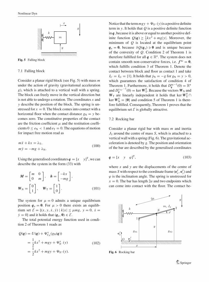
Fig. 5 Falling block

7.1 Falling block

Consider a planar rigid block (see Fig. 5) with mass munder the action of gravity (gravitational acceleration

g), which is attached to a vertical wall with a spring.

The block can freely move in the vertical direction but

is not able to undergo a rotation. The coordinates x and

y describe the position of the block. The spring is un-

stressed for x = 0. The block comes into contact with a

horizontal floor when the contact distance gN = y be-

comes zero. The constitutive properties of the contact

are the friction coefficient μ and the restitution coeffi-

cients 0 ≤ eN < 1 and eT = 0. The equations of motion

for impact free motion read as

mx + kx = λT,

my = −mg + λN.(100)

Using the generalised coordinates q = [x y]T, we can

describe the system in the form (33) with

M =[

m 0

0 m

], h =

[−kx−mg

],

WN =[

0

1

], WT =

[1

0

]. (101)

The system for μ = 0 admits a unique equilibrium

position qe = 0. For μ > 0 there exists an equilib-

rium set E = {(x, y, x, y) | k|x | ≤ μmg, y = 0, x =y = 0} and it holds that (qe, 0) ∈ E .

The total potential energy function used in condi-

tion 2 of Theorem 1 reads as

Q(q) = U (q) + �∗CN

(gN(q))

= 1

2kx2 + mgy + �∗

R− (y)

= 1

2kx2 + mgy + �R+ (y).

(102)

Notice that the term mgy + �R+ (y) is a positive definite

term in y. It holds that Q is a positive definite function

in q, because it is above or equal to another positive def-

inite function Q(q) ≥ 12kx2 + mg|y|. Moreover, the

minimum of Q is located at the equilibrium point

qe = 0, because ∂ Q(qe) � 0 and is unique because

of the convexity of Q. Condition 2 of Theorem 1 is

therefore fulfilled for all q ∈ Rn . The system does not

contain smooth non-conservative forces, i.e. f nc = 0,

which fulfills condition 3 of Theorem 1. Denote the

contact between block and floor as contact 1 and take

IC = IG = {1}. It holds that γN = −g for gN = y > 0,

which guarantees the satisfaction of condition 4 of

Theorem 1. Furthermore, it holds that Dncq

−1(0) = Rn

and DλT Cq

−1(0) = ker WT

T. Because the vectors WN and

WT are linearly independent it holds that ker WTT ∩

ker WTN = {0} and condition 5 of Theorem 1 is there-

fore fulfilled. Consequently, Theorem 1 proves that the

equilibrium set E is globally attractive.

7.2 Rocking bar

Consider a planar rigid bar with mass m and inertia

JS around the centre of mass S, which is attached to a

vertical wall with a spring (Fig. 6). The gravitational ac-

celeration is denoted by g. The position and orientation

of the bar are described by the generalised coordinates

q = [x y ϕ]T, (103)

where x and y are the displacements of the centre of

mass S with respect to the coordinate frame (eIx , eI

y) and

ϕ is the inclination angle. The spring is unstressed for

x = 0. The bar has length 2a and two endpoints which

can come into contact with the floor. The contact be-

Fig. 6 Rocking bar

Springer

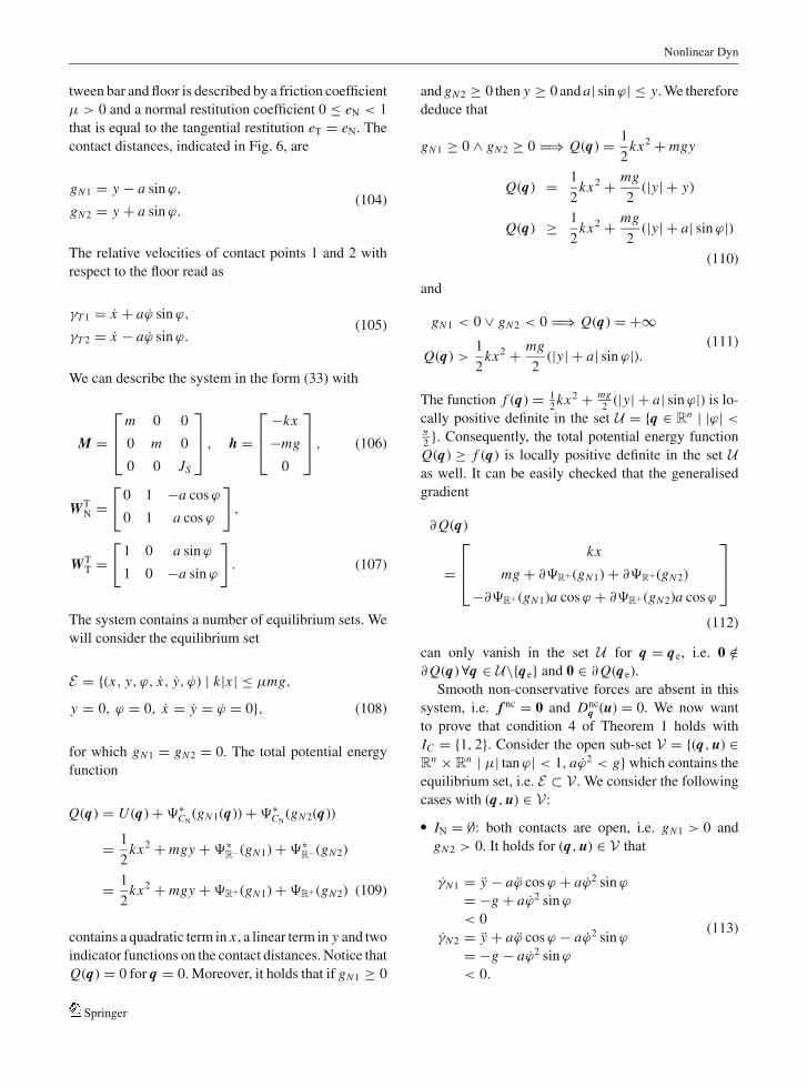
Nonlinear Dyn

tween bar and floor is described by a friction coefficient

μ > 0 and a normal restitution coefficient 0 ≤ eN < 1

that is equal to the tangential restitution eT = eN. The

contact distances, indicated in Fig. 6, are

gN1 = y − a sin ϕ,

gN2 = y + a sin ϕ.(104)

The relative velocities of contact points 1 and 2 with

respect to the floor read as

γT 1 = x + aϕ sin ϕ,

γT 2 = x − aϕ sin ϕ.(105)

We can describe the system in the form (33) with

M =

⎡⎢⎣ m 0 0

0 m 0

0 0 JS

⎤⎥⎦ , h =

⎡⎢⎣ −kx

−mg

0

⎤⎥⎦ , (106)

WTN =

[0 1 −a cos ϕ

0 1 a cos ϕ

],

WTT =

[1 0 a sin ϕ

1 0 −a sin ϕ

]. (107)

The system contains a number of equilibrium sets. We

will consider the equilibrium set

E = {(x, y, ϕ, x, y, ϕ) | k|x | ≤ μmg,

y = 0, ϕ = 0, x = y = ϕ = 0}, (108)

for which gN1 = gN2 = 0. The total potential energy

function

Q(q) = U (q) + �∗CN

(gN1(q)) + �∗CN

(gN2(q))

= 1

2kx2 + mgy + �∗

R− (gN1) + �∗R− (gN2)

= 1

2kx2 + mgy + �R+ (gN1) + �R+ (gN2) (109)

contains a quadratic term in x , a linear term in y and two

indicator functions on the contact distances. Notice that

Q(q) = 0 for q = 0. Moreover, it holds that if gN1 ≥ 0

and gN2 ≥ 0 then y ≥ 0 and a| sin ϕ| ≤ y. We therefore

deduce that

gN1 ≥ 0 ∧ gN2 ≥ 0 =⇒ Q(q) = 1

2kx2 + mgy

Q(q) = 1

2kx2 + mg

2(|y| + y)

Q(q) ≥ 1

2kx2 + mg

2(|y| + a| sin ϕ|)

(110)

and

gN1 < 0 ∨ gN2 < 0 =⇒ Q(q) = +∞

Q(q) >1

2kx2 + mg

2(|y| + a| sin ϕ|).

(111)

The function f (q) = 12kx2 + mg

2(|y| + a| sin ϕ|) is lo-

cally positive definite in the set U = {q ∈ Rn | |ϕ| <π2}. Consequently, the total potential energy function

Q(q) ≥ f (q) is locally positive definite in the set Uas well. It can be easily checked that the generalised

gradient

∂ Q(q)

=

⎡⎢⎣ kx

mg + ∂�R+ (gN1) + ∂�R+ (gN2)

−∂�R+ (gN1)a cos ϕ + ∂�R+ (gN2)a cos ϕ

⎤⎥⎦(112)

can only vanish in the set U for q = qe, i.e. 0 /∈∂ Q(q) ∀q ∈ U\{qe} and 0 ∈ ∂ Q(qe).

Smooth non-conservative forces are absent in this

system, i.e. f nc = 0 and Dncq (u) = 0. We now want

to prove that condition 4 of Theorem 1 holds with

IC = {1, 2}. Consider the open sub-set V = {(q, u) ∈Rn × Rn | μ| tan ϕ| < 1, aϕ2 < g} which contains the

equilibrium set, i.e. E ⊂ V . We consider the following

cases with (q, u) ∈ V:� IN = ∅: both contacts are open, i.e. gN1 > 0 and

gN2 > 0. It holds for (q, u) ∈ V that

γN1 = y − aϕ cos ϕ + aϕ2 sin ϕ

= −g + aϕ2 sin ϕ

< 0

γN2 = y + aϕ cos ϕ − aϕ2 sin ϕ

= −g − aϕ2 sin ϕ

< 0.

(113)

Springer

Nonlinear Dyn� IN = {1}: contact 1 is closed and contact 2 is open,

i.e. gN1 = 0 and gN2 > 0. We consider contact 1 to be

closed for a nonzero time-interval. The normal con-

tact acceleration of the closed contact 1 must vanish:

γN1 = y − aϕ cos ϕ + aϕ2 sin ϕ

0 = −g + 1

mλN1 + a2

JScos2 ϕ λN1

−a2

JScos ϕ sin ϕ λT 1 + aϕ2 sin ϕ

0 = −g +(

1

m+ a2

JScos ϕ(cos ϕ − μ sin ϕ)

)λN1

+ aϕ2 sin ϕ,

(114)

with λT 1 = μλN1, i.e. μ ∈ −μ Sign(γT 1). It follows

from (114) that the normal contact force λN1 is a

function of ϕ and ϕ. The contact acceleration of con-

tact 2 therefore becomes

γN2 = y + aϕ cos ϕ − aϕ2 sin ϕ

= −g + 1

mλN1 − a2

JScos2 ϕ λN1

+ a2

JScos ϕ sin ϕ λT 1 − aϕ2 sin ϕ

= −g +(

1

m− a2

JScos ϕ(cos ϕ − μ sin ϕ)

)λN1

− aϕ2 sin ϕ

=1m − a2

JScos ϕ(cos ϕ − μ sin ϕ)

1m + a2

JScos ϕ(cos ϕ − μ sin ϕ)

(g − aϕ2 sin ϕ)

− g − aϕ2 sin ϕ

= −2ga2 m

JScos ϕ(cos ϕ − μ sin ϕ)

1 + a2 mJS

cos ϕ(cos ϕ − μ sin ϕ)

− 2aϕ2 sin ϕ

1 + a2 mJS

cos ϕ(cos ϕ − μ sin ϕ). (115)

Using |μ| ≤ μ and (q, u) ∈ V it follows that γN2 <

0.� IN = {2}: contact 1 is open and contact 2 is closed,

i.e. gN1 > 0 and gN2 = 0. Similar to the previous

case we can prove that γN1 < 0.

Hence, there exists a non-empty set IC = {1, 2}, such

that γNi (q, u) < 0 (a.e.) for ∀i ∈ IC\IN and ∀(q, u) ∈V . Condition 4 of Theorem 1 is therefore fulfilled.

It holds that Dncq

−1(0) = Rn and using Proposition 3

it follows that DλTq

−1(0) = ker WT

T(q). Furthermore, for

q ∈ C = {q ∈ Rn | gN1 = gN2 = 0} follows the impli-

cation WTN(q)u = 0 =⇒ y = 0 ∧ ϕ = 0 and similarly

WTT(q)u = 0 =⇒ x = 0. We conclude that there is al-

ways dissipation when both contacts are closed and

u �= 0 because

ker WTT(q) ∩ ker WT

N (q) = {0} ∀q ∈ C, (116)

and condition 5 of Theorem 1 is therefore fulfilled.

The largest level set of V = T (q, u) + Q(q) which lies

entirely inQ = {(q, u) ∈ Rn × Rn | q ∈ U} is given by

V (q, u) < mga. The largest level set of V which lies

entirely in V is determined by V (q, u) < 12

JSga and

V (q, u) <mga√1+μ2

. We therefore choose the set Iρ∗ as

Iρ∗ = {(q, u) ∈ Rn × Rn | V (q, u) < ρ∗}, with

ρ∗ = min

(1

2JS

g

a,

mga√1 + μ2

). (117)

If additionally

1

2

(μmg)2

k< ρ∗, (118)

then it holds that E ⊂ Iρ∗ . We conclude that Theorem 1

proves conditionally the local attractivity of the equi-

librium set E and that Iρ∗ is a conservative estimate

of the region of attraction. Naturally, the attractivity is

only local, because the system has also other attractive

equilibrium sets for ϕ = nπ with n ∈ Z and unstable

equilibrium sets around ϕ = π2

+ nπ .

7.3 Rocking block

The theory presented in this paper has been applied

in the Section 7.2 to a simple rocking bar system. In

this Section we study a rocking block on a rigid floor,

which seems like a slight modification of the previ-

ous example, but which shows that the analysis can

already become very elaborate for a relatively simple

system.

Consider a planar rigid block with mass m and inertia

JS around the centre of mass S, which is attached to

a vertical wall with a spring (Fig. 7). The block has a

hight 2b, a width 2a and the gravitational acceleration

is denoted by g. The position and orientation of the

Springer

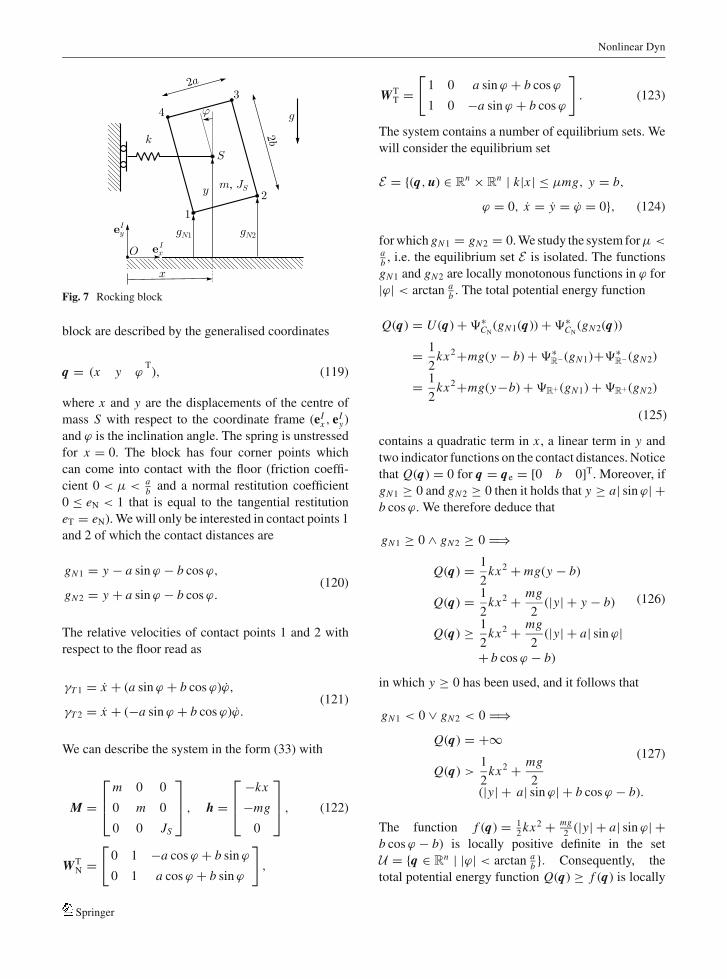
Nonlinear Dyn

Fig. 7 Rocking block

block are described by the generalised coordinates

q = (x y ϕT), (119)

where x and y are the displacements of the centre of

mass S with respect to the coordinate frame (eIx , eI

y)

and ϕ is the inclination angle. The spring is unstressed

for x = 0. The block has four corner points which

can come into contact with the floor (friction coeffi-

cient 0 < μ < ab and a normal restitution coefficient

0 ≤ eN < 1 that is equal to the tangential restitution

eT = eN). We will only be interested in contact points 1

and 2 of which the contact distances are

gN1 = y − a sin ϕ − b cos ϕ,

gN2 = y + a sin ϕ − b cos ϕ.(120)

The relative velocities of contact points 1 and 2 with

respect to the floor read as

γT 1 = x + (a sin ϕ + b cos ϕ)ϕ,

γT 2 = x + (−a sin ϕ + b cos ϕ)ϕ.(121)

We can describe the system in the form (33) with

M =

⎡⎢⎣ m 0 0

0 m 0

0 0 JS

⎤⎥⎦ , h =

⎡⎢⎣ −kx

−mg

0

⎤⎥⎦ , (122)

WTN =

[0 1 −a cos ϕ + b sin ϕ

0 1 a cos ϕ + b sin ϕ

],

WTT =

[1 0 a sin ϕ + b cos ϕ

1 0 −a sin ϕ + b cos ϕ

]. (123)

The system contains a number of equilibrium sets. We

will consider the equilibrium set

E = {(q, u) ∈ Rn × Rn | k|x | ≤ μmg, y = b,

ϕ = 0, x = y = ϕ = 0}, (124)

for which gN1 = gN2 = 0. We study the system for μ <ab , i.e. the equilibrium set E is isolated. The functions

gN1 and gN2 are locally monotonous functions in ϕ for

|ϕ| < arctan ab . The total potential energy function

Q(q) = U (q) + �∗CN

(gN1(q)) + �∗CN

(gN2(q))

= 1

2kx2+mg(y − b) + �∗

R− (gN1)+�∗R− (gN2)

= 1

2kx2+mg(y−b) + �R+ (gN1) + �R+ (gN2)

(125)

contains a quadratic term in x , a linear term in y and

two indicator functions on the contact distances. Notice

that Q(q) = 0 for q = qe = [0 b 0]T. Moreover, if

gN1 ≥ 0 and gN2 ≥ 0 then it holds that y ≥ a| sin ϕ| +b cos ϕ. We therefore deduce that

gN1 ≥ 0 ∧ gN2 ≥ 0 =⇒

Q(q) = 1

2kx2 + mg(y − b)

Q(q) = 1

2kx2 + mg

2(|y| + y − b)

Q(q) ≥ 1

2kx2 + mg

2(|y| + a| sin ϕ|

+ b cos ϕ − b)

(126)

in which y ≥ 0 has been used, and it follows that

gN1 < 0 ∨ gN2 < 0 =⇒Q(q) = +∞

Q(q) >1

2kx2 + mg

2(|y| + a| sin ϕ| + b cos ϕ − b).

(127)

The function f (q) = 12kx2 + mg

2(|y| + a| sin ϕ| +

b cos ϕ − b) is locally positive definite in the set

U = {q ∈ Rn | |ϕ| < arctan ab }. Consequently, the

total potential energy function Q(q) ≥ f (q) is locally

Springer

Nonlinear Dyn

positive definite in the set U as well. It can be easily

checked that the generalised gradient

∂ Q(q) =

⎡⎢⎢⎢⎣kx

mg + ∂�R+ (gN1) + ∂�R+ (gN2)

−∂�R+ (gN1)(a cos ϕ − b sin ϕ)

+ ∂�R+ (gN2)(a cos ϕ + b sin ϕ)

⎤⎥⎥⎥⎦(128)

can only vanish in the set U for q = qe, i.e. 0 /∈∂ Q(q) ∀q ∈ U\{qe} and 0 ∈ ∂ Q(qe).

Smooth non-conservative forces are absent in this

system, i.e. f nc = 0 and Dncq (u) = 0. We now want

to prove that condition 4 of Theorem 1 holds with

IC = {1, 2}. Consider the open sub-set V = {(q, u) ∈Rn × Rn | d(ϕ) > 0,

√a2 + b2ϕ2 < g} with d(ϕ) =

a cos ϕ − b sin ϕ − μ(a sin ϕ + b cos ϕ). The set V is

a neighbourhood of the equilibrium set, i.e. E ⊂ V . We

consider the following cases with (q, u) ∈ V:� IN = ∅: both contacts are open, i.e. gN1 > 0 and

gN2 > 0. It holds for (q, u) ∈ V that

γN1 = y + (−a cos ϕ + b sin ϕ)ϕ

+ (a sin ϕ + b cos ϕ)ϕ2

= −g + (a sin ϕ + b cos ϕ)ϕ2

< 0

γN2 = y + (a cos ϕ + b sin ϕ)ϕ

+ (−a sin ϕ + b cos ϕ)ϕ2

= −g + (−a sin ϕ + b cos ϕ)ϕ2

< 0.

(129)

� IN = {1}: contact 1 is closed and contact 2 is open,

i.e. gN1 = 0 and gN2 > 0. We consider contact 1 to be

closed for a nonzero time-interval. The normal con-

tact acceleration of the closed contact 1 must vanish:

γN1 = y + (−a cos ϕ + b sin ϕ)ϕ

+ (a sin ϕ + b cos ϕ)ϕ2

0 = −g + 1

mλN1 + 1

JS(−a cos ϕ + b sin ϕ)2λN1

+ 1

JS(−a cos ϕ + b sin ϕ)(a sin ϕ

+ b cos ϕ)λT 1 + (a sin ϕ + b cos ϕ)ϕ2

0 = −g +(

1

m+ 1

JS(−a cos ϕ + b sin ϕ)(−a cos ϕ

+ b sin ϕ + μ(a sin ϕ + b cos ϕ))

)λN1

+ (a sin ϕ + b cos ϕ)ϕ2

0 = −g +(

1

m+ 1

JS(a cos ϕ − b sin ϕ)d(ϕ)

)λN1

+ (a sin ϕ + b cos ϕ)ϕ2, (130)

with d(ϕ) = a cos ϕ − b sin ϕ − μ(a sin ϕ + b cos ϕ)

and λT 1 = μλN1, i.e. μ ∈ −μ Sign(γT 1), from which

follows the normal contact force λN1 as a function

of ϕ and ϕ. The contact acceleration of contact 2

therefore becomes

γN2 = y + (a cos ϕ + b sin ϕ)ϕ + (−a sin ϕ

+ b cos ϕ)ϕ2

= −g + 1

mλN1 + 1

JS(a cos ϕ + b sin ϕ)

× (−a cos ϕ + b sin ϕ)λN1

+ 1

JS(a cos ϕ + b sin ϕ)(a sin ϕ

+ b cos ϕ)λT 1 + (−a sin ϕ + b cos ϕ)ϕ2

= −g+(

1

m− 1

JS(a cos ϕ+b sin ϕ)d(ϕ)

)λN1

+ (−a sin ϕ + b cos ϕ)ϕ2

=1 − m

JS(a cos ϕ + b sin ϕ)d(ϕ)

1 + mJS

(a cos ϕ − b sin ϕ)d(ϕ)(g − (a sin ϕ

+ b cos ϕ)ϕ2) − g+(−a sin ϕ+b cos ϕ)ϕ2

= −2 m

JSad(ϕ)(g cos ϕ − bϕ2) + 2aϕ2 sin ϕ

1 + mJS

(a cos ϕ − b sin ϕ)d(ϕ).

(131)

Using gN1 = 0 and gN2 > 0 we deduce that sin ϕ >

0. Moreover, using (q, u) ∈ V it follows that

| tan ϕ| <a−bμ

b+aμand ϕ2 < g/

√a2 + b2. We study the

system for μ < ab , i.e. the equilibrium set E is iso-

lated. Hence, it must hold that cos ϕ > b√a2+b2

. From

d(ϕ) > 0 and |μ| ≤ μ it follows that d(ϕ) > 0. Sub-

stitution of ϕ2 < g/√

a2 + b2 and cos ϕ > b√a2+b2

gives g cos ϕ − bϕ2 > 0. Because d(ϕ) > 0, cos ϕ >b√

a2+b2, sin ϕ > 0 and a cos ϕ − b sin ϕ > 0 it fol-

lows that γN2 < 0.� IN = {2}: contact 1 is open and contact 2 is closed,

i.e. gN1 > 0 and gN2 = 0. Similar to the previous

case we can prove that γN1 < 0.

Springer

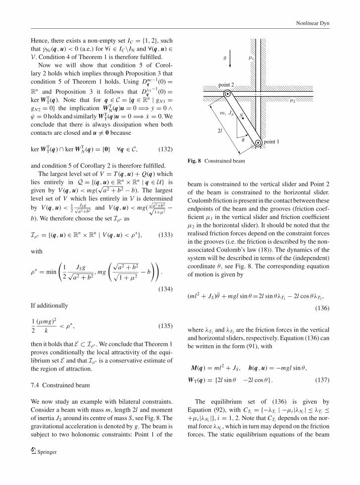
Nonlinear Dyn

Hence, there exists a non-empty set IC = {1, 2}, such

that γNi (q, u) < 0 (a.e.) for ∀i ∈ IC\IN and ∀(q, u) ∈V . Condition 4 of Theorem 1 is therefore fulfilled.

Now we will show that condition 5 of Corol-

lary 2 holds which implies through Proposition 3 that

condition 5 of Theorem 1 holds. Using Dncq

−1(0) =Rn and Proposition 3 it follows that DλT

q−1

(0) =ker WT

T(q). Note that for q ∈ C = {q ∈ Rn | gN1 =gN2 = 0} the implication WT

N(q)u = 0 =⇒ y = 0 ∧ϕ = 0 holds and similarly WT

T(q)u = 0 =⇒ x = 0. We

conclude that there is always dissipation when both

contacts are closed and u �= 0 because

ker WTT(q) ∩ ker WT

N (q) = {0} ∀q ∈ C, (132)

and condition 5 of Corollary 2 is therefore fulfilled.

The largest level set of V = T (q, u) + Q(q) which

lies entirely in Q = {(q, u) ∈ Rn × Rn | q ∈ U} is

given by V (q, u) < mg(√

a2 + b2 − b). The largest

level set of V which lies entirely in V is determined

by V (q, u) < 12

JS g√a2+b2

and V (q, u) < mg(√

a2+b2√1+μ2

−b). We therefore choose the set Iρ∗ as

Iρ∗ = {(q, u) ∈ Rn × Rn | V (q, u) < ρ∗}, (133)

with

ρ∗ = min

(1

2

JSg√a2 + b2

, mg

(√a2 + b2√1 + μ2

− b

)).

(134)

If additionally

1

2

(μmg)2

k< ρ∗, (135)

then it holds that E ⊂ Iρ∗ . We conclude that Theorem 1

proves conditionally the local attractivity of the equi-

librium set E and that Iρ∗ is a conservative estimate of

the region of attraction.

7.4 Constrained beam

We now study an example with bilateral constraints.

Consider a beam with mass m, length 2l and moment

of inertia JS around its centre of mass S, see Fig. 8. The

gravitational acceleration is denoted by g. The beam is

subject to two holonomic constraints: Point 1 of the

Fig. 8 Constrained beam

beam is constrained to the vertical slider and Point 2

of the beam is constrained to the horizontal slider.

Coulomb friction is present in the contact between these

endpoints of the beam and the grooves (friction coef-

ficient μ1 in the vertical slider and friction coefficient

μ2 in the horizontal slider). It should be noted that the

realised friction forces depend on the constraint forces

in the grooves (i.e. the friction is described by the non-

associated Coulomb’s law (18)). The dynamics of the

system will be described in terms of the (independent)

coordinate θ , see Fig. 8. The corresponding equation

of motion is given by

(ml2 + JS)θ + mgl sin θ =2l sin θλT1− 2l cos θλT2

,

(136)

where λT1and λT2

are the friction forces in the vertical

and horizontal sliders, respectively. Equation (136) can

be written in the form (91), with

M(q) = ml2 + JS, h(q, u) = −mgl sin θ,

WT(q) = [2l sin θ −2l cos θ ] . (137)

The equilibrium set of (136) is given by

Equation (92), with CTi = {−λTi | −μi |λNi | ≤ λTi ≤+μi |λNi |}, i = 1, 2. Note that CTi depends on the nor-

mal force λNi , which in turn may depend on the friction

forces. The static equilibrium equations of the beam

Springer

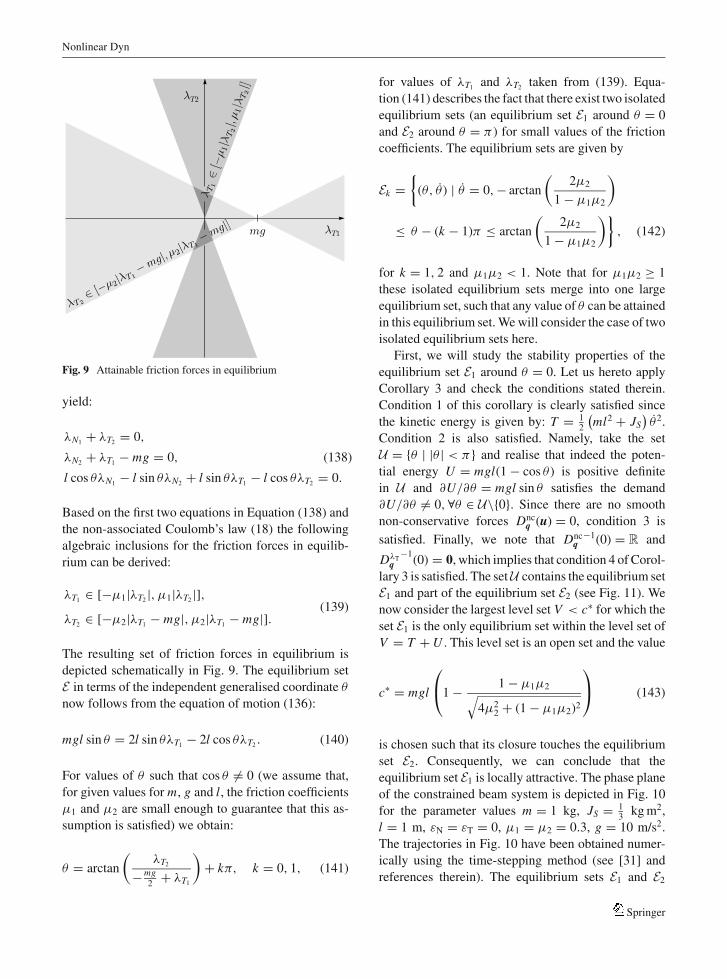
Nonlinear Dyn

Fig. 9 Attainable friction forces in equilibrium

yield:

λN1+ λT2

= 0,

λN2+ λT1

− mg = 0,

l cos θλN1− l sin θλN2

+ l sin θλT1− l cos θλT2

= 0.

(138)

Based on the first two equations in Equation (138) and

the non-associated Coulomb’s law (18) the following

algebraic inclusions for the friction forces in equilib-

rium can be derived:

λT1∈ [−μ1|λT2

|, μ1|λT2|],

λT2∈ [−μ2|λT1

− mg|, μ2|λT1− mg|].

(139)

The resulting set of friction forces in equilibrium is

depicted schematically in Fig. 9. The equilibrium set

E in terms of the independent generalised coordinate θ

now follows from the equation of motion (136):

mgl sin θ = 2l sin θλT1− 2l cos θλT2

. (140)

For values of θ such that cos θ �= 0 (we assume that,

for given values for m, g and l, the friction coefficients

μ1 and μ2 are small enough to guarantee that this as-

sumption is satisfied) we obtain:

θ = arctan

(λT2

−mg2

+ λT1

)+ kπ, k = 0, 1, (141)

for values of λT1and λT2

taken from (139). Equa-

tion (141) describes the fact that there exist two isolated

equilibrium sets (an equilibrium set E1 around θ = 0

and E2 around θ = π ) for small values of the friction

coefficients. The equilibrium sets are given by

Ek ={

(θ, θ ) | θ = 0, − arctan

(2μ2

1 − μ1μ2

)≤ θ − (k − 1)π ≤ arctan

(2μ2

1 − μ1μ2

)}, (142)

for k = 1, 2 and μ1μ2 < 1. Note that for μ1μ2 ≥ 1

these isolated equilibrium sets merge into one large

equilibrium set, such that any value of θ can be attained

in this equilibrium set. We will consider the case of two

isolated equilibrium sets here.

First, we will study the stability properties of the

equilibrium set E1 around θ = 0. Let us hereto apply

Corollary 3 and check the conditions stated therein.

Condition 1 of this corollary is clearly satisfied since

the kinetic energy is given by: T = 12

(ml2 + JS

)θ2.

Condition 2 is also satisfied. Namely, take the set

U = {θ | |θ | < π} and realise that indeed the poten-

tial energy U = mgl(1 − cos θ ) is positive definite

in U and ∂U/∂θ = mgl sin θ satisfies the demand

∂U/∂θ �= 0, ∀θ ∈ U\{0}. Since there are no smooth

non-conservative forces Dncq (u) = 0, condition 3 is

satisfied. Finally, we note that Dncq

−1(0) = R and

DλTq

−1(0) = 0, which implies that condition 4 of Corol-

lary 3 is satisfied. The setU contains the equilibrium set

E1 and part of the equilibrium set E2 (see Fig. 11). We

now consider the largest level set V < c∗ for which the

set E1 is the only equilibrium set within the level set of

V = T + U . This level set is an open set and the value

c∗ = mgl

⎛⎝1 − 1 − μ1μ2√4μ2

2 + (1 − μ1μ2)2

⎞⎠ (143)

is chosen such that its closure touches the equilibrium

set E2. Consequently, we can conclude that the

equilibrium set E1 is locally attractive. The phase plane

of the constrained beam system is depicted in Fig. 10

for the parameter values m = 1 kg, JS = 13

kg m2,

l = 1 m, εN = εT = 0, μ1 = μ2 = 0.3, g = 10 m/s2.

The trajectories in Fig. 10 have been obtained numer-

ically using the time-stepping method (see [31] and

references therein). The equilibrium sets E1 and E2

Springer

Nonlinear Dyn

Fig. 10 Phase plane andthe set in whichV = T + U < c∗

Fig. 11 Schematic representation of the set U in which V ≥ 0(V as in Equation (144))

are indicated by thick lines on the axis θ = 0. It can

be seen in Fig. 10 that the level set V < c∗ is a fairly

good (though conservative) estimate for the region of

attraction of the equilibrium set E1.

Secondly, we will study the stability properties of the

equilibrium set E2 around θ = π . We apply Theorem 2

and check the conditions stated therein. The function

V in this theorem is chosen as follows:

V = −1

2(JS + ml2)θ2 + mgl (1 + cos θ ) , (144)

where V ≥ 0 ∈ U with the set U depicted schemati-

cally in Fig. 11. The time-derivative of V obeys

V = −θWTλT = −γTTλT,

with WT = [2l sin θ − 2l cos θ ], λTT = [λT1

λT2]

and γT = WTTθ = [2l θ sin θ − 2l θ cos θ ]T are the

sliding velocities in the two frictional sliders. Note that

V ≥ 0 for all (θ, θ ) ∈ U and V = 0 if and only if θ = 0.

We can easily show that solutions cannot stay in S\E2,

with S = {(θ, θ ) | θ = 0}, using the equation of mo-

tion (136). The conditions of statement 3 of Theorem 2

are satisfied and it can be concluded that the equilib-

rium set E2 is unstable.

The equilibrium set E2 becomes a saddle point for

μ1,2 = 0. This saddle structure in the phase plane (see

Fig. 10) remains for μ1,2 > 0, but E2 is a set instead

of a point. Interestingly, the stable manifold of E2

is ‘thick’, i.e. there exists a bundle of solutions (de-

picted in dark grey) which are attracted to the unsta-

ble equilibrium set E2. Put differently: the equilibrium

set E2 has a region of attraction, where the region is

a set with a non-empty interior. The unstable half-

manifolds of E2 originate at the tips of the set E2 and

are heteroclinic orbits with the stable equilibrium set

E1.

8 Conclusions

In this paper, conditions are given under which the equi-

librium set of multi-degree-of-freedom non-linear me-

chanical systems with an arbitrary number of frictional

Springer

Nonlinear Dyn

unilateral constraints is attractive. The theorems for

attractivity are proved by using the framework of mea-

sure differential inclusions together with a Lyapunov-

type stability analysis and a generalisation of LaSalle’s

invariance principle for non-smooth systems. The total

mechanical energy of the system, including the sup-

port function of the normal contact forces, is chosen

as Lyapunov function. It has been proved that, under

some conditions, the differential measure of the Lya-

punov function is non-positive, which is basically a dis-

sipativity argument. Sufficient conditions for the dis-

sipativity of frictional unilateral constraints are given.

If we do not consider dependent constraints, then the

restitution coefficients must either be small enough, or,

be all equal to each other. The latter condition has also

been stated in [19, 35]. Attractivity of the equilibrium

set is proved in Theorem 1 under a number of condi-

tions. Condition 4 is a condition, which is difficult to

satisfy and check. It guarantees that there exists no in-

variant set when one or more contacts are open. Still,

we are able to use Theorem 1 to prove the attractivity

of equilibrium sets in a number of example systems

in Section 7. Moreover, we provide conservative es-

timates for the region of attraction of the equilibrium

set.

Non-linear mechanical systems with frictional bilat-

eral constraints form a sub-class of the class of systems

that can be studied with Theorem 1. For this sub-class

of systems the (local) attractivity of the equilibrium

set can be proven with Corollary 3. Moreover, a re-

sult on the instability of equilibrium sets of differen-

tial inclusions is proposed in Section 6.2. This result

allows us to investigate the instability of equilibrium

sets of non-linear mechanical systems with frictional

bilateral constraints. An example system with two fric-

tional bilateral constraints is studied in Section 7.4 and

the attractivity and instability of its equilibrium sets are

discussed. Figure 10 showed that the stable manifold

of a ‘saddle-type’ equilibrium set consists of a bundle

of solutions, which are attracted to the unstable equi-

librium set in finite time.

The theorems presented in this paper have been

proved for dissipative systems and form the stepping

stone to the analysis of non-dissipative systems for

which the equilibrium set might still be attractive due to

the dissipation of the frictional impacts (see also [45]).

The results of this paper will be used in further research

to develop control methods for systems with unilateral

constraints.

Appendix A: Positive definite matrices

Proposition 4. Let A ∈ Rn×n be a symmetric positivedefinite matrix and B ∈ Rn×n be a diagonal positivedefinite matrix with the diagonal elements bii whichfulfil 1 ≥ bii ≥ bmin > 0, i = 1, . . . , n. If

1 − bmin <1

cond(A)

then it holds that the matrix AB is positive definite.

Proof: The matrix A = AT > 0 has real positive

eigenvalues and it therefore holds that

xT Ax ≥ λmin‖x‖2 , (145)

where λmin is the smallest eigenvalue of A. Moreover,

it holds that

xT A(I − B)x ≤ |xT A(I − B)x|≤ |A| |I − B| ‖x‖2

≤ λmax(1 − bmin)‖x‖2 ,

(146)

where λmax is the largest eigenvalue of A and bmin is

the smallest diagonal element of B. Using the above

inequalities, we deduce that

xT ABx = xT(A − A(I − B))x≥ (λmin − λmax(1 − bmin)) ‖x‖2 .

(147)

Hence, if it holds that

1 − bmin <λmin

λmax

=:1

cond(A), (148)

then it follows that xT ABx > 0 holds for all x �= 0. �

Appendix B: Convex analysis

The generalised differential of a scalar convex function,

defined by Equation (149), is called the subdifferential

∂ f (x) = {y | f (x∗) ≥ f (x)

+ yT(x∗ − x); ∀x∗} ⊂ Rn. (149)

Springer

Nonlinear Dyn

Let C be a convex set and x ∈ C . The set of vectors ythat are normal to x ∈ C form the normal cone of C in x

NC (x) = {y | yT(x∗ − x) ≤ 0, x ∈ C, ∀x∗ ∈ C}.(150)

If x is in the interior of C then NC (x) = 0. If x /∈ C then

NC (x) = ∅. The indicator function of C is defined as

�C (x) ={

0, x ∈ C,

+∞, x /∈ C.(151)

The indicator function is a convex function. With the

definition of the subdifferential (149) and the indicator

function it follows that

∂�C (x) = {y | �C (x∗) ≥ �C (x) + yT(x∗ − x),

x ∈ C, ∀x∗ ∈ C}= {y | 0 ≥ yT(x∗ − x), x ∈ C, ∀x∗ ∈ C}.

(152)

This is exactly the definition of the normal cone at C .

The subdifferential of the indicator function at x ∈ Cis therefore the normal cone of C at x,

∂�C (x) = NC (x). (153)

Let f be a convex function. The function f ∗ is called

the conjugate function of f and is defined as

f ∗(x∗) = supx

{xTx∗ − f (x)}. (154)

From Fenchel’s inequality [42] follows the equality

xTx∗ = f (x) + f ∗(x∗) ⇐⇒ x∗

∈ ∂ f (x) ⇐⇒ x ∈ ∂ f ∗(x∗). (155)

The conjugate function of the indicator function �C

on a convex set C is called support function,

�∗C (x∗) = sup

x{xTx∗ − �C (x)}

= supx

{xTx∗ | x ∈ C}. (156)

The support function is positively homogeneous in the

sense that

�∗C (ax∗) = a�∗

C (x∗) ∀a > 0. (157)

If x ∈ ∂�∗C (x∗) then it holds that x ∈ C and

xTx∗ = �C (x)︸ ︷︷ ︸=0

+ �∗C (x∗)

= �∗C (x∗).

(158)

It follows that ∂�∗C (0) = C . The support function

�∗C (x∗) is a convex function with �∗

C (0) = 0. Hence,

if 0 ∈ C , then 0 ∈ ∂�∗C (0) from which follows that

�∗C (x∗) attains a minimum at x∗ = 0, i.e.

0 ∈ C =⇒ �∗C (x∗) ≥ 0. (159)

Moreover, if 0 ∈ int C then it follows that �∗C (x∗)

attains a global minimum at x∗ = 0, i.e.

0 ∈ int C =⇒ �∗C (x∗) > 0 ∀x∗ �= 0. (160)

Appendix C: Subderivative

The differentiablility of a function f : Rn → R at a

point x is connected with the existence of a tan-

gent hyperplane to the graph of f at the point

(x, f (x)) [41]. The concept of differentiablity can be

generalised by considering the contingent cone to the

epigraph of f instead. In this section, we consider

a lower semi-continuous extended function f : Rn →R ∪ {∞} whose domain dom( f ) = {x ∈ Rn | f (x) <

∞} is non-empty (i.e. the function is not trivial). The

epigraph of the function f is closed, because f is lower

semi-continuous. Various generalised notions of gra-

dients exist, but the subderivative is the most natural

object to focus on and is often called the contingent

epiderivative [5] or epicontingent derivative [4].

We define the function

d f (x)(v) = lim inft↓0, v ′→v

f (x + tv ′) − f (x)

t

as the subderivative of f at x in the direction v [42].

The epigraph of d f (x)(·) is the contingent cone at the

Springer

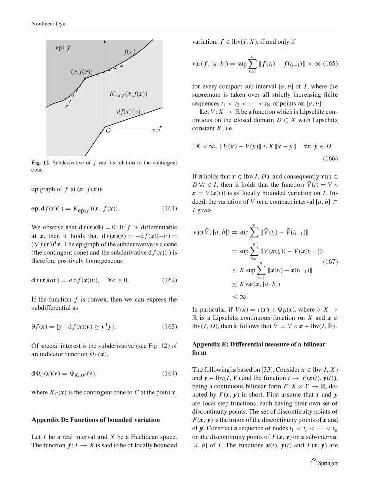
Nonlinear Dyn

Fig. 12 Subderivative of f and its relation to the contingentcone

epigraph of f at (x, f (x))

epi d f (x)(·) = Kepi f ((x, f (x)) . (161)

We observe that d f (x)(0) = 0. If f is differentiable

at x, then it holds that d f (x)(v) = −d f (x)(−v) =(∇ f (x))Tv . The epigraph of the subderivative is a cone

(the contingent cone) and the subderivative d f (x)(·) is

therefore positively homogeneous

d f (x)(av) = a d f (x)(v), ∀a ≥ 0. (162)

If the function f is convex, then we can express the

subdifferential as

∂ f (x) = {y | d f (x)(v) ≥ vT y}. (163)

Of special interest is the subderivative (see Fig. 12) of

an indicator function �C (x),

d�C (x)(v) = �KC (x)(v), (164)

where KC (x) is the contingent cone to C at the point x.

Appendix D: Functions of bounded variation

Let I be a real interval and X be a Euclidean space.

The function f : I → X is said to be of locally bounded

variation, f ∈ lbv(I, X ), if and only if

var( f , [a, b]) = supn∑

i=1

‖ f (ti ) − f (ti−1)‖ < ∞ (165)

for every compact sub-interval [a, b] of I , where the

supremum is taken over all strictly increasing finite

sequences t1 < t2 < · · · < tN of points on [a, b].

Let V : X → R be a function which is Lipschitz con-

tinuous on the closed domain D ⊂ X with Lipschitz

constant K , i.e.

∃K <∞, ‖V (x) − V (y)‖≤ K‖x − y‖ ∀x, y ∈ D.

(166)

If it holds that x ∈ lbv(I, D), and consequently x(t) ∈D ∀t ∈ I , then it holds that the function V (t) = V ◦x = V (x(t)) is of locally bounded variation on I . In-

deed, the variation of V on a compact interval [a, b] ⊂I gives

var(V , [a, b]) = supn∑

i=1

‖V (ti ) − V (ti−1)‖

= supn∑

i=1

‖V (x(ti )) − V (x(ti−1))‖

≤ K supn∑

i=1

‖x(ti ) − x(ti−1)‖≤ K var(x, [a, b])

< ∞.

(167)

In particular, if V (x) = v(x) + �D(x), where v: X →R is a Lipschitz continuous function on X and x ∈lbv(I, D), then it follows that V = V ◦ x ∈ lbv(I, R).

Appendix E: Differential measure of a bilinearform

The following is based on [33]. Consider x ∈ lbv(I, X )

and y ∈ lbv(I, Y ) and the function t → F(x(t), y(t)),being a continuous bilinear form F : X × Y → R, de-

noted by F(x, y) in short. First assume that x and yare local step functions, each having their own set of

discontinuity points. The set of discontinuity points of

F(x, y) is the union of the discontinuity points of x and

of y. Construct a sequence of nodes t1 < tt < · · · < tnon the discontinuity points of F(x, y) on a sub-interval

[a, b] of I . The functions x(t), y(t) and F(x, y) are

Springer

Nonlinear Dyn

therefore constant on each open sub-interval (ti , ti+1).

The differential measure dF(x, y) equals the sum of a

locally finite collection of point measures placed at the

discontinuity points of F

∫[a,b]

dF(x, y) =n∑

i=1

(F(x+(ti ), y+(ti ))

−F(x−(ti ), y−(ti ))). (168)

Similarly, dx equals the sum of point measures placed

at the nodes ti with values x+(ti ) − x−(ti ) (and the same

applies for dy). It therefore holds that

∫[a,b]

F(dx, y−) =n∑

i=1

F(x+(ti ) − x−(ti ), y−(ti )),∫[a,b]

F(x+, dy) =n∑

i=1

F(x+(ti ), y+(ti ) − y−(ti )).

(169)

Exploiting the bilinearity of F yields

∫[a,b]

dF(x, y) =∫

[a,b]

(F(dx, y−) + F(x+, dy)).

(170)

Every locally bounded function can be approximated

by a local step function and their difference can be

made arbitrarily small by refining the partition of the

local step function. Equation (170) does therefore not

only hold for local step functions, but holds for arbitrary

locally bounded functions x and y, as has been proved

rigourously in [33].

Consider now a symmetric quadratic form G(x) =F(x, x) = xT Ax, with A = AT. We deduce from

Equation (170) that

∫[a,b]

dG(x) =∫

[a,b]

(F(dx, x−) + F(x+, dx))

=∫

[a,b]

F(x+ + x−, dx)

=∫

[a,b]

(x+ + x−)T A dx (171)

or simply dG = (x+ + x−)T A dx.

References

1. Adly, S., Goeleven, D.: A stability theory for second-ordernonsmooth dynamical systems with application to frictionproblems. J. Mathematiques Pures et Appliquees 83, 17–51(2004)

2. Alvarez, J., Orlov, I., Acho, L.: An invariance principlefor discontinuous dynamic systems with application to aCoulomb friction oscillator. J. Dyn. Syst. Meas. Control 122,687–690 (2000)

3. Anosov, D.V.: Stability of the equilibrium positions in relaysystems. Autom. Remote Control 20, 130–143 (1959)

4. Aubin, J.-P., Ekeland, I.: Applied Nonlinear Analysis. Pureand Applied Mathematics. Wiley, Berlin (1984)

5. Aubin, J.-P., Frankowska, H.: Set-Valued Analysis, vol. 2,Systems and Control: Foundations and Applications.Birkhauser, Boston (1990)

6. Bacciotti, A., Ceragioli, F.: Stability and stabilization of dis-continuous systems and nonsmooth Lyapunov functions. ES-IAM: Control Optim. Calculus Variations 4, 361–376 (1999)

7. Bainov, D.D., Simeonov, P.S.: Systems with Impulse Effect:Stability, Theory and Applications. Wiley, New York (1989)

8. Brogliato, B.: Nonsmooth Mechanics, 2nd edn. Springer,London (1999)

9. Brogliato, B.: Absolute stability and the Lagrange–Dirichlettheorem with monotone multivalued mappings. Syst. ControlLett. 51, 343–353 (2004)

10. Brogliato, B., Goeleven, D.: The Krakovskii–LaSalle invari-ance principle for a class of unilateral dynamical systems.Math. Control Signals Syst. 17(1), 57–76 (2005)

11. Brogliato, B., Niculescu, S.-I., Orhant, P.: On the control offinite-dimensional mechanical systems with unilateral con-straints. IEEE Trans. Autom. Control 42(2), 200–215 (1997)

12. Camlibel, M., Heemels, W., van der Schaft, A., Schumacher,J.: Switched networks and complementarity. IEEE Trans.Circuits Syst. 50(8), 1036–1046 (2003)

13. Chareyron, S., Wieber, P.B.: A LaSalle’s invariance the-orem for nonsmooth Lagrangian dynamical systems. In:Proceedings of the ENOC-2005 Conference, 7–12 August,Eindhoven, The Netherlands (2005)

14. Chareyron, S., Wieber, P.B.: Stability and regulation of non-smooth dynamical systems. IEEE Trans. Autom. Control(2007) submitted

15. Davrazos, G.N., Koussoulas, N.T.: A review of stabilityresults for switched and hybrid systems. In: 9th Mediter-ranean Conference on Control and Automation, 27–29 June,Dubrovnik, Croatia (2001)

16. Filippov, A.F.: Differential Equations with Discontinu-ous Right-hand Sides. Kluwer Academic, Dordrecht, TheNetherlands (1988)

17. Glocker, Ch.: On frictionless impact models in rigid-bodysystems. Phil. Trans. R. Soc. Lond. A 359, 2385–2404(2001)

18. Glocker, Ch.: Set-Valued Force Laws, Dynamics of Non-Smooth Systems, vol. 1, Lecture Notes in Applied Mechan-ics. Springer-Verlag, Berlin (2001)

19. Glocker, Ch.: An introduction to impacts. In: Haslinger, J.,Stavroulakis, G.E. (eds.), Nonsmooth Mechanics of Solids,vol. 485, CISM Courses and Lectures. Springer, Wien, NewYork, pp. 45–101 (2006)

Springer

Nonlinear Dyn

20. Goeleven, D., Brogliato, B.: Stability and instability matri-ces for linear evolution variational inequalities. IEEE Trans.Autom. Control 49, 521–534 (2004)

21. Goeleven, D., Brogliato, B.: Necessary conditions of asymp-totic stability for unilateral dynamical systems. NonlinearAnal. 61(6), 961–1004 (2005)

22. Haslinger, J., Stavroulakis, G.E. (eds.): Nonsmooth Mechan-ics of Solids, vol. 485, CISM Courses and Lectures. Springer,Wien, New York (2006)

23. Johansson, M., Rantzer, A.: Computation of piecewisequadratic Lyapunov functions for hybrid systems. IEEETrans. Autom. Control 43(4), 555–559 (1998)

24. Kane, T.R., Levinson, D.A.: Dynamics, Theory and Appli-cations. McGraw-Hill, New York (1985)

25. Khalil, H.K.: Nonlinear Systems. Prentice-Hall, EnglewoodCliffs, NJ (1996)

26. Kunze, M.: Non-Smooth Dynamical Systems. Springer,Berlin (2000)

27. Leine, R.I.: Bifurcations in discontinuous mechanical sys-tems of Filippov-type. Ph.D. Thesis, Eindhoven Universityof Technology, The Netherlands (2000)

28. Leine, R.I.: On the stability of motion in non-smooth me-chanical systems. Habilitation Thesis, ETH Zurich, Switzer-land (2007)

29. Leine, R.I., Brogliato, B., Nijmeijer, H.: Periodic motion andbifurcations induced by the Painleve paradox. Eur. J. Mech.A Solids 21(5), 869–896 (2002)

30. Leine, R.I., Glocker, Ch.: A set-valued force law for spatialCoulomb–Contensou friction. Eur. J. Mech. A Solids 22,193–216 (2003)

31. Leine, R.I., Nijmeijer, H.: Dynamics and Bifurcations ofNon-Smooth Mechanical Systems, vol. 18, Lecture Notesin Applied and Computational Mechanics. Springer-Verlag,Berlin (2004)

32. Moreau, J.J.: Liaisons unilaterales sans frottement et chocsinelastiques. Comptes Rendu des Seances de l’Academie desSciences 296, 1473–1476 (1983)

33. Moreau, J.J.: Bounded variation in time. In: Moreau, J.J.,Panagiotopoulos, P.D., Strang, G. (eds.), Topics in Non-smooth Mechanics, pp. 1–74. Birkhauser Verlag, Basel,Boston, Berlin (1988)

34. Moreau, J.J.: Unilateral contact and dry friction in finite free-dom dynamics. In: Moreau, J.J., Panagiotopoulos, P.D. (eds.)Non-Smooth Mechanics and Applications, vol. 302, CISM

Courses and Lectures, pp. 1–82. Springer, Wien, New York(1988)

35. Moreau, J.J.: Some numerical methods in multibody dynam-ics: Application to granular materials. Eur. J. Mech. A Solids13(4, suppl.), 93–114 (1994)

36. Papastavridis, J. G.: Analytical Mechanics: A Comprehen-sive Treatise on the Dynamics of Constrained Systems: ForEngineers, Physicists and Mathematicians. Oxford Univer-sity Press, New York (2002)

37. Payr, M., Glocker, C.: Oblique frictional impact of a bar:Analysis and comparison of different impact laws. NonlinearDyn. 41, 361–383 (2005)

38. Pettersson, S., Lennartson, B.: Hybrid system stability androbustness verification using linear matrix inequalities. Int.J. Control 75(16–17), 1335–1355 (2002)

39. Pfeiffer, F., Glocker, Ch.: Multibody Dynamics with Unilat-eral Contacts. Wiley, New York (1996)

40. Quittner, P.: An instability criterion for variational inequali-ties. Nonlinear Anal. 15(12), 1167–1180 (1990)

41. Rockafellar, R.T.: The Theory of Subgradients and its Appli-cations to Problems of Optimization. Convex and NonconvexFunctions, vol. 1, Research and Education in Mathematics.Heldermann Verlag, Berlin (1970)

42. Rockafellar, R.T., Wets, R.-B.: Variational Analysis.Springer, Berlin (1998)

43. Shevitz, D., Paden, B.: Lyapunov stability of nonsmoothsystems. IEEE Trans. Autom. Control 39(9), 1910–1914(1994)

44. Tornambe, A.: Modeling and control of impact in mechan-ical systems: theory and experimental results. IEEE Trans.Autom. Control 44(2), 294–309 (1999)

45. Van de Wouw, N., Leine, R.I.: Attractivity of equilibrium setsof systems with dry friction. Int. J. Nonlinear Dyn. ChaosEng. Syst. 35(1), 19–39 (2004)

46. van de Wouw, N., van den Heuvel, M., van Rooij, J.,Nijmeijer, H.: Performance of an automatic ball balancerwith dry friction. Int. J. Bif. Chaos 15(1), 65–82 (2005)

47. Yakubovich, V.A., Leonov, G.A., Gelig, A.K.: Stability ofStationary Sets in Control Systems with Discontinuous Non-linearities, vol. 14, Series on Stability, Vibration and Controlof Systems, Series A. World Scientific, Singapore (2004)

48. Ye, H., Michel, A., Hou, L.: Stability theory for hybrid dy-namical systems. IEEE Trans. Autom. Control 43(4), 461–474 (1998)

Springer