STABILITY AND THE DISTRIBUTION OF POWER 1996.pdf · World Politics 48 (January 1996), 239–67 STABILITY AND THE DISTRIBUTION OF POWER By ROBERT POWELL* THE relation between the distribution

World Politics 48 ( January 1996), 239–67

STABILITY AND THEDISTRIBUTION OF POWER

By ROBERT POWELL*

THE relation between the distribution of power and the probabilityof war has been at the center of a long and important debate in in-

ternational relations theory. Is an even distribution of power more orless stable than a preponderance of power? The balance-of-powerschool generally argues that an even distribution of power is more sta-ble, whereas the preponderance-of-power school generally argues theopposite, that a preponderance of power is more stable.1

Empirical efforts to resolve this debate have yielded equivocal re-sults. Siverson and Tennefoss, for example, find an even distribution ofpower to be more stable, whereas Kim and Moul find a preponderanceof power to be more stable. Singer, Bremer, and Stuckey find an evendistribution to be more stable than a preponderance of power duringthe nineteenth century and the opposite during the twentieth century.Maoz and Bueno de Mesquita and Lalman, by contrast, find no signif-icant relation between the probability of war and the distribution ofpower. Finally, Mansfield finds evidence of a nonlinear, quadratic rela-tion in which the probability of war is smallest when there is an evendistribution and a preponderance of power.2

* I am grateful to Bruce Bueno de Mesquita, James Fearon, Joanne Gowa, Robert Keohane, JamesMorrow, Paul Papayoanou, Leo Simon, R. Harrison Wagner, and Barry Weingast for their commentsand criticisms. This work was assisted by a grant from the National Science Foundation (SES9121959) and a National Fellowship at the Hoover Institution at Stanford University.

1 Arguing that a balance is more stable are Innis Claude, Power and International Relations (NewYork: Random House, 1962); Hans Morgenthau, Politics among Nations, 4th ed. (New York: AlfredKnopf, 1967); John Mearsheimer, “Back to the Future,’’ International Security 15 (Summer 1990);Quincy Wright, A Study of War (Chicago: University of Chicago Press, 1965); and Arnold Wolfers,Discord and Collaboration (Baltimore: Johns Hopkins University Press, 1962). Arguing that a prepon-derance is more stable are Geoffrey Blainey, The Causes of War (New York: Free Press, 1973); A. F. K.Organski, World Politics (New York: Alfred A. Knopf, 1968); and A. F. K. Organski and Jacek KuglerThe War Ledger (Chicago: University of Chicago Press, 1980). For a review of this debate, see JackLevy, “The Causes of War: A Review of Theories and Evidence,’’ in Philip Tetlock et al., eds., Behav-ior, Society, and Nuclear War, vol. 1 (New York: Oxford University Press, 1989); for a discussion of someof the important conceptual issues, see R. Harrison Wagner, “Peace, War, and the Balance of Power,”American Political Science Review 88 (September 1994).

2 Randolph Siverson and Michael Tennefoss, “Power, Alliance, and the Escalation of InternationalConflict, 1815–1965,’’ American Political Science Review 78 (December 1984); Woosang Kim, “AllianceTransitions and Great Power War,’’ American Journal of Political Science 35 (November 1991); idem,

Aileen

Claims about the relation between the distribution of power and thelikelihood of war have generally lacked any formal foundations. Somerecent work has attempted to fill this gap, however. Bueno de Mesquitaand Lalman and Fearon analyze models of international bargaining.The former find, first, that the probability of war is smallest when thedistribution of power is uneven and, second, that “dissatisfaction withthe status quo is unrelated to the likelihood of war.”3 Fearon, by con-strast, finds that the probability of war is independent of the distribu-tion of power; that is, a change in the distribution of power has noeffect on the likelihood of war.4

This essay examines the relation between the probability of war andthe distribution of power in the context of a game-theoretic model inwhich two states are bargaining about revising the international statusquo. In the model the states make proposals for changing the statusquo. The bargaining continues until the states reach a mutually accept-able settlement or until one of them becomes sufficiently pessimisticabout the prospects of reaching an agreement that it uses force to try toimpose a new international order. The states’ equilibrium strategiesspecify the demands the states will make of each other and the circum-stances in which they will resort to force. The equilibrium strategiesthus make it possible to calculate the probability that bargaining willbreak down in war as a function of the distribution of power betweenthe two states. The shape of this function can then be compared to therelation claimed to exist by the balance-of-power and preponderance-of-power schools.

The probability of war in the model turns out to be a function of thedisparity between the status quo distribution of benefits and the distri-bution expected to result from the use of force. The outcome expectedfrom using force is, in turn, directly related to the distribution of power.

“Power Transitions and Great Power War from Westphalia to Waterloo,’’ World Politics 45 (October1992); William Moul, “Balances of Power and the Escalation to War of Serious International Disputesamong the European Great Powers, 1815–1939,’’ American Journal of Political Science 32 (February1988); J. David Singer, Stuart Bremer, and John Stuckey, “Capability Distribution, Uncertainty, andMajor Power War, 1820–1965,’’ in Bruce Russett, ed., Peace, War, and Numbers (Beverly Hills, Calif.:Sage, 1972); Zeev Maoz, “Resolve, Capabilities, and the Outcomes of Interstate Disputes,1815–1976,’’ Journal of Conflict Resolution 27 ( June 1983); Bruce Bueno de Mesquita and David Lal-man, “Empirical Support for Systemic and Dyadic Explanations of International Conflict,’’ World Pol-itics 41 (October 1988); idem, Reason and War (New Haven: Yale University Press, 1992); EdwardMansfield, “The Concentration of Capabilities and the Onset of War,’’ Journal of Conflict Resolution 36(March 1992); idem, Power, Trade, and War (Princeton: Princeton University Press, 1994).

3 Bueno de Mesquita and Lalman (fn. 2, 1992), 204–5, 190.4 James Fearon, “War, Relative Power, and Private Information’’ (Paper presented at the annual

meeting of the International Studies Association, Atlanta, March 31–April 4, 1992), 20.

240 WORLD POLITICS

Thus, the probability of war is a function of the disparity between thestatus quo and the distribution of power. When this disparity is small,the division of benefits expected from the use of force is approximatelythe same as the existing status quo distribution. The gains to usingforce are therefore too small to outweigh the costs of fighting. Neitherstate is willing to use force to change the status quo, and the probabil-ity of war is zero. When the disparity between the status quo division ofbenefits and the distribution of power is large, then at least one state iswilling to use force to overturn the status quo. Moreover, as the dispar-ity grows, the probability of war generally increases.

These results seem quite intuitive: as the disparity between the dis-tribution of power and the distribution of benefits grows, the probabil-ity of war generally increases. Indeed, this formal result echoes Gilpin’sexplanation of hegemonic wars.5 Such wars arise, he argues, because ofa disparity between the distribution of power and the international sta-tus quo distribution of benefits imposed by the hegemon following theprevious hegemonic war.6 Although intuitive, these results contradictthe expectations of both the balance-of-power and preponderance-of-power schools. The former expects the probability of war to be smallestwhen power is evenly distributed, but the probability of war is smallestin the present model when the distribution of power mirrors the statusquo distribution of territory. These claims will coincide only in the spe-cial case in which the status quo distribution is even. The preponder-ance-of-power school expects the probability of war to be smallestwhen the distribution of power is highly skewed and to increase as thedistribution of power becomes more even. But the probability of war islargest in the model developed below when the distribution of power ishighly skewed.

The formal results derived here also differ from those obtained byFearon and Bueno de Mesquita and Lalman. Unlike Fearon, the prob-ability of war in the present formulation does vary with changes in thedistribution of power.7 Unlike Bueno de Mesquita and Lalman, whofind that “dissatisfaction with the status quo is unrelated to the likeli-hood of war’’ and that the probability of war declines as the distribu-

5 Robert Gilpin, War and Change in World Politics (Cambridge: Cambridge University Press, 1981).6 Although the potential use of force is not the source of the coercive pressure, some suggest that in-

ternational regimes are more likely to break down when the underlying distribution of power differsfrom the distribution of benefits the regime confers. See Robert Keohane and Joseph Nye, Power andInterdependence (Boston: Little Brown, 1977), 139; and Stephen Krasner, “Regimes and the Limits ofRealism,” in Krasner, ed., International Regimes (Ithaca, N.Y.: Cornell University Press, 1983), 357–58,

7 Fearon (fn. 4).

STABILITY & THE DISTRIBUTION OF POWER 241

tion of power becomes more skewed, the probability of war is directlyrelated to the level of dissatisfaction with the status quo and generallyincreases as the distribution of power becomes more skewed.8

The remainder of this essay is organized as follows. The next sectionmotivates and defines the model and discusses some qualifications andlimitations. The subsequent section describes the game’s equilibrium.The final section uses this equilibrium to specify the probability of waras a function of the distribution of power and compares these resultswith the expectations of the balance-of-power and preponderance-of-power schools and with other formal work. That section also offers apossible explanation for the equivocal empirical results of efforts tomeasure the relation between stability and the distribution of power.

THE MODEL

To motivate the model, suppose two states are bargaining about revis-ing the international status quo. More concretely, imagine that twostates are negotiating about changing the territorial status quo. Eachstate proposes a division of the territory that the other state can acceptor reject. The bargaining continues with offer followed by counterofferuntil the states agree on a proposed division or until one of the statesbecomes sufficiently pessimistic about the prospects of reaching a mu-tually acceptable settlement that it resorts to force to try to impose anew territorial settlement.9

How do changes in the distribution of power between these twostates affect the bargaining and, more specifically, the probability thatthe bargaining will break down in war? Are the negotiations more likelyto break down if one state has a preponderance of power or if there isan even distribution of power? It might seem at first that the prepon-derance-of-power school is clearly correct and that the bargaining isless likely to break down if one of the states has a preponderance ofpower. That is, suppose a state, say S1, has just proposed a particular di-vision to the other state S2. S2 would be tempted to use force to imposea settlement rather than accept S1’s offer only if the expected payoff tousing force were at least as large as the payoff to agreeing to the pro-posal. But the weaker S2, the lower its expected payoff to fighting. In-

8 Bueno de Mesquita and Lalman (fn. 2, 1992), 190, 204–5.9 In a more general model the two states might be bargaining about altering the international sta-

tus quo where the set of feasible outcomes is an n-dimensional policy space. Each point in this spacerepresents a different international order and a different distribution of benefits for the two states. Theformal analysis developed below applies equally well to this more general formulation.

242 WORLD POLITICS

deed, if S2 is sufficiently weak, its payoff to using force will be less thanits payoff to agreeing to S1’s offer. In this case, S2 will acquiesce to S1’sdemand and will not be tempted to use force. Nor will S1 be tempted touse force, since S2 is willing to agree to S1’s demand. This reasoning,which suggests that a preponderance of power will be more stable, is es-sentially the reasoning Organski advances: “A preponderance of power. . . increases the chances of peace, for the greatly stronger side need notfight at all to get what it wants, while the weaker side would be plainlyfoolish to attempt battle for what it wants.’’10

There is, however, a countervailing factor at work. The preceding ar-gument was based on the assumption that S1’s proposal was fixed. Butas S1 becomes stronger and S2 becomes weaker, S1 knows that S2 is morelikely to accept any given proposal. Thus, S1 will demand more of S2 asS2 becomes weaker. S2, in turn, may be more likely to resist these largerdemands, and war may become more likely when there is a preponder-ance of power. If so, then a preponderance of power would be less stable.By contrast, an even distribution of power would restrain all states’demands and thereby enhance stability. This restraining effect of aneven distribution of power underlies the balance-of-power school’sanalysis of the relation between stability and the distribution of power.As Wolfers argues, “Thus, from the point of view of preserving thepeace . . . it may be a valid proposition that a balance of power placingrestraint on every nation is more advantageous in the long run than thehegemony even of those deemed peace-loving at the time.’’11

In sum, a shift in the balance of power against S2 has two competingeffects. First, S2 is more likely to accept any specific demand. But, sec-ond, more will be demanded of it than would have been had it beenmore powerful. The first effect tends to make war less likely, while thesecond tends to make war more likely. The net result of these two op-posing effects on the probability of war is unclear: whereas the prepon-derance-of-power school emphasizes the first effect, the balance-of-power school underscores the second effect. The game-theoretic modelof bargaining developed here makes it possible to weigh the interactionof these two competing effects more formally.

Rubinstein’s seminal analysis of an alternating-offer, infinite-horizonbargaining game provides a point of departure for the present analy-sis.12 In Rubinstein’s model two actors are trying to divide a pie. Oneactor begins the game by proposing a division of the pie to the other,

10 Organski (fn. 1), 294.11 Wolfers (fn. 1), 120. See also Claude (fn. 1), 62.12 Ariel Rubinstein, “Perfect Equilibrium in a Bargaining Model,’’ Econometrica 50 ( January 1982).


who can either accept or reject the offer. Acceptance ends the game andthe pie is divided as agreed. If the second actor rejects the initial pro-posal, it makes a counteroffer that the first actor can either accept or re-ject. Acceptance again ends the game. If the first actor rejects theproposal, it makes a new offer. The actors alternate making offers untilthey agree on a division.13

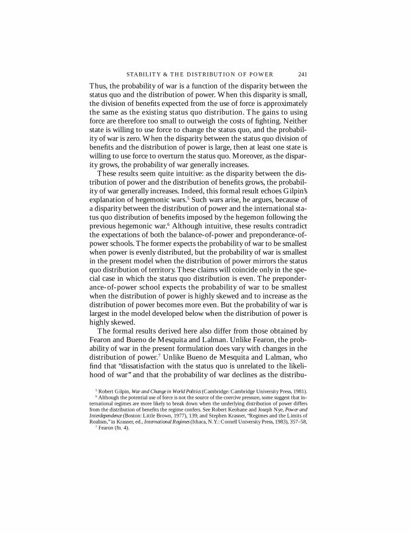
The present model adds the option of using force to Rubinstein’sbasic structure. As illustrated in Figure 1, S1 begins the game byproposing a division of the status quo. More formally, S1 demands somefraction x of the disputed territory where x lies between zero and one.If, for example, S1 sets x = 1, then S1 is demanding all of the territory foritself; if S1 sets x = 1/2, it is demanding half of the territory; and if S1sets x = 0, it is offering S2 all of the territory. (The arc between “0’’ and“1’’ in Figure 1 indicates that a state can demand any fraction between0 and 1.) S2 can accept this offer by saying yes, which is denoted by Y;reject it by saying no, N, and subsequently make a counteroffer; or forcea settlement by attacking S1 with A. The game ends if S2 accepts or at-tacks. If S2 rejects, it then proposes a new territorial division. S1 can nowaccept, reject, or attack. As before, accepting or attacking ends thegame. If S1 rejects, it again suggests another division. The bargainingcontinues, possibly forever, with offers alternating back and forth untilone of the states accepts a proposal or attacks.

To specify the states’ payoffs, let (q, 1 – q) denote the status quo di-vision where q and 1 – q are S1’s and S2’s respective shares. Now supposethat the states agree to divide the territory according to (x, 1 – x) whereS1 and S2 receive x and 1 – x, respectively. Assume further that thisagreement is reached at time t, that is, after t + 1 offers. (For notationalconvenience, the first offer is made at time t = 0.) If agreement isreached at time t, then S1 had q and S2 had 1 – q from the beginning ofthe game until time t – 1. The payoff that S1 derives from having a flowof q for the first t periods will be taken to be U1(q) + δU1(q) + δ 2U1(q) + ... + δ t – 1U1(q) = (1 – δ t )U1(q)/(1 – δ ) where δ is the states’common discount factor and U1 is S1’s utility function for benefits. S1will also be assumed to prefer larger allocations to smaller allocationsbut with a nonincreasing marginal value.14 Once agreement is reachedat time t, S1’s allocation from time t forward is x. The present value ofhaving x from time t forward is δ tU1(x) + δ t + 1U1(x) + δ t + 2U1(x) + ... =δ tU1(x)/(1 – δ ) . Thus, S1’s payoff to agreeing to (x, 1 – x) at time t is (1 – δ t)U1(q)/(1 – δ ) + δ tU1(x)/(1 – δ ) . Similarly, S2’s payoff to agree-

13 Rubinstein (fn. 12) showed that this game has a unique subgame-perfect equilibrium.14 More formally, U1 is assumed to be twice differentiable with U1' > 0 and U1" ≤ 0. S1 is risk neutral

if U1" = 0 and risk averse if U1" < 0.

244 WORLD POLITICS

FIG

UR

E1

AN

INFI

NIT

E-H

OR

IZO

N,A

LTE

RN

AT

ING

-OFF

ER

GA

ME

WIT

HT

HE

OP

TIO

NO

FU

SIN

GFO

RC

E

ing to (x, 1 – x) at time t is (1 – δ t)U2(1 – q)/(1 – δ ) + δ tU2(1 – x)/(1 –δ ) where U2 is S2’s utility.

To define the states’ payoffs if they fail to reach an agreement andone of them uses force, suppose that they fight at time t. As before, S1derives (1 – δ t)U1(q)/(1 – δ ) from having q during the first t periods.To simplify the specification of S1’s payoff following an attack, war willbe assumed to end in one of only two ways. Either S1 will be completelyvictorious, or S2 will be. (The limitations of this simplification are dis-cussed below.) If S1 prevails, it takes all of the territory at a cost of fight-ing c1. The payoff to having all of the territory less the cost of fightingfrom time t forward is δ t(U1(1) – c1) + δ t + 1(U1(1) – c1) + δ t + 2(U1(1) – c1)+ ... = δ t(U1(1) – c1)/(1 – δ) . If S1 loses, S2 captures all of the territorywhich leaves S1 with nothing but the cost of fighting. The payoff to thisoutcome is δ t(U1(0) – c1) + δ t + 1(U1(0) – c1) + δ t + 2(U1(0) – c1) + ... = δ t

(U1(0) – c1)/(1 – δ ) .Going to war is an uncertain venture. Let p reflect the balance of

power or the distribution of capabilities between S1 and S2. That is, p,which is assumed to be common knowledge, is the probability that S1will prevail if force is used.15 Then S1’s expected payoff to a bargainingprocess that ends in war at time t is the value of living with the statusquo until time t – 1 plus the payoff to prevailing at time t times theprobability of prevailing, p, plus the payoff to losing at time t times theprobability of losing, 1 – p:

This payoff can be simplified by normalizing the utility function by set-ting the payoff to having all of the territory equal to one and the payoffto having no territory equal to zero (that is, U1(1) = 1 and U1(0) = 0).Letting W1(t) and W2(t) denote S1’s and S2’s normalized payoffs to abargaining process that ends in war at time t leaves:

246 WORLD POLITICS

15 There are no offensive or defensive advantages in the present formulation, so it makes no differ-ence whether S1 or S2 attacks.

(1 – δ t)U1(q) + p

δ t(U1(1) – c1) + (1 – p)δ t(U1(0) – c1) .

1 – δ 1 – δ 1 – δ

W1(t) = 1 – δ t

U1(q) + δ t

( p – c1)1 – δ 1 – δ( )

W2(t) = 1 – δ t

U2(1 – q) + δ t

( 1 – p – c2 ) .1 – δ 1 – δ( )

The model developed so far has complete information. Each stateknows the other state’s payoffs. As discussed more fully below, as longas information is complete, bargaining never breaks down, regardless ofthe distribution of power. In this model incomplete information is aprerequisite to war. In the next section each state is assumed to be un-certain of the other’s willingness to use force.

Before turning to incomplete information and an analysis of thegame’s equilibrium, however, it will be useful to consider some of thelimitations and qualifications of the model. The most significant limi-tation is that there are only two states. One argument about the rela-tion between stability and the distribution of power emphasizes theimportance of the number of coalitions that could form to block anystate’s bid for hegemony. The larger the number of states and the moreeven the distribution of power, the larger the number of potentialblocking coalitions and the less likely is war.16 As a formal analysis ofthis argument clearly requires a model in which there are more thantwo actors, it is beyond the scope of the present analysis.17

It is important to emphasize, however, that although some argu-ments about the relation between the distribution of power and theprobability of war presuppose the existence of more than two states,other arguments do not. Wright, for example, explicitly considers thesituation in which there are only two states. In this case, balance-of-power theory expects that “there would be great instability unless [thetwo states] were very nearly equal in power or their frontiers werewidely separated or difficult to pass.”18 Similarly, Mearsheimer consid-ers the case of two great powers and claims that a balance of power ismore stable: “Power can be more or less equally distributed among themajor powers of both bipolar and multipolar systems. Both are morepeaceful when equality is greatest among the poles.’’19 In sum, the con-flicting claims of the balance-of-power and preponderance-of-powerschools apply to systems in which there are only two states, as well as tosystems with more than two states. The present analysis focuses on theformer case.

A second significant limitation of the model is that the distributionof power is fixed. But the key to several arguments about the relation

16 See Levy (fn. 1), 231–32; Mansfield (fn. 2, 1994), 17–18; and Wright (fn. 1), 755.17 For efforts to examine the relation between stability and the distribution of power in a setting in

which there are more than two states, see Emerson Niou and Peter Ordeshook, “Stability in AnarchicInternatonal Systems,’’ American Journal of Political Science 84 (December 1990); Wagner (fn. 1); andidem, “The Theory of Games and the Balance of Power,’’ World Politics 38 ( July 1986).

18 Wright (fn. 1), 755.19 Mearsheimer (fn. 1), 18; emphasis added.


between the likelihood of war and the distribution of power is that thisdistribution shifts over time, perhaps because of uneven economicgrowth.20 This raises an important problem, which is the effects ofchanges in the distribution of power over time on the probability ofwar. Unfortunately, it is beyond the scope of the present model andmust await future work.21

Another seeming limitation is that war can result in only two possi-ble outcomes: a state either wins all of the territory or loses all of it.This limitation is more apparent than real, however. The assumptionthat war can end in only two ways simplifies the notation and discus-sion, but it is not central to the analysis of the model. One might as-sume instead that war could result in any territorial division. Changesin the distribution of power would still be reflected in changes in theprobability distribution over the now larger set of possible outcomes.

Furthermore, both states are assumed to agree on the distribution ofpower (that is, both states know p). This assumption not only simplifiesthe analysis but has some substantive import for international relationstheory as well. Blainey and others argue that war results from uncer-tainty about the distribution of power.22 While this uncertainty may bean important cause of war, it is not a necessary condition as Blaineysuggests. The model serves as a counterexample to this claim: statesagree on the distribution of power and yet there is war.23

Finally, the terms of the agreement do not affect the distribution ofpower. So, for example, an agreement that transfers a large amount ofterritory to one state does not make that state more powerful. Wagnerargues that this may be an important cause of war, and extending themodel to allow for this possibility would be relatively straightforward.24

THE EQUILIBRIUM

This section characterizes the game’s equilibrium. To summarize theresults, a state will be called dissatisfied if it prefers fighting to the sta-tus quo and satisfied if it prefers the status quo to fighting. If both states

20 See, for example, Charles Doran and Wes Parsons, “War and the Cycle of Relative Power,’’ Amer-ican Political Science Review 74 (December 1980); Gilpin (fn. 5); Organski (fn. 1); and Organski andKugler (fn. 1).

21 For efforts in this direction, see Fearon (fn. 4); Woosang Kim and James Morrow, “When DoPower Transitions Lead to War?’’ American Journal of Political Science 36 (November 1992); and Pow-ell, “Appeasement as a Game of Timing” (Manuscript, Department of Political Science, University ofCalifornia, Berkeley, July 1995).

22 Blainey (fn. 1).23 Fearon (fn. 4) first makes and develops this point.24 Wagner (fn. 1).

248 WORLD POLITICS

are satisfied, then the status quo remains unchanged and the probabil-ity of war is zero, as neither state can credibly threaten to use force tooverturn the status quo. If one of the states is dissatisfied, then the sat-isfied state makes its optimal offer to the dissatisfied state given the sat-isfied state’s beliefs about the willingness of the dissatisfied state to useforce. Although the dissatisfied state can always reject this offer andmake a counteroffer, it never does so in equilibrium. Rather, the dissat-isfied state either accepts this offer or attacks.25 The next section usesthese equilibrium strategies to calculate the probability of war as a func-tion of the distribution of power. (Readers less interested in the deriva-tion of these results may omit the rest of this section.)

Three preliminaries are needed before the equilibrium strategies canbe specified. First, a dissatisfied state must be defined more precisely.Second, the equilibrium of the complete-information game must bedescribed. Finally, incomplete information needs to be introduced.

A state is dissatisfied if it prefers fighting to living with the statusquo. In symbols, S1’s payoff to fighting now (that is, at t = 0) is W1(0) =(p – c1)/(1 – δ ). S1’s payoff to living with the status quo is U1(q)/(1 – δ ). Thus, S1 is dissatisfied if p – c1 > U1(q). Similarly, S2 is dissatis-fied if 1 – p – c2 > U2(1 – q). At most only one state can be dissatisfied.26

The complete-information game has a very simple equilibrium.27 Ifboth states are satisfied, then neither state can credibly threaten to useforce to change the status quo. The status quo remains unaltered. If oneof the states is dissatisfied, then the satisfied state offers just enough inequilibrium to the dissatisfied state to ensure that it will never findfighting worthwhile. In effect, the satisfied state appeases the dissatis-fied state by offering it just enough to leave it indifferent between ac-cepting the offer and fighting. In symbols, suppose that S1 is thedissatisfied state. Then the satisfied state, S2, will offer just enough, sayx, so that the dissatisfied state’s payoff to accepting x, U1(x)/(1 – δ ) , isequal to the payoff to fighting, (p – c1)/(1 – δ ). Thus, x satisfies U1(x) =p – c1. To see that this is S2’s optimal offer, note that S2 would never

25 As will be seen, at most only one state can be dissatisfied.26 This follows from the assumptions that the states are risk neutral or risk averse, that they agree on

the distribution of power, and that fighting is costly. Because the states are risk neutral or risk averse,the utility functions are concave, which implies U1(q) ≥ q and U2(1 – q) ≥ 1 – q. If both states are dis-satisfied, then p – c1 > U1(q) ≥ q and 1 – p – c2 > U2 (1 – q) ≥ 1 – q. Adding these inequalities gives 1 –c1 – c2 > 1 or 0 > c1 + c2 . But fighting is costly, so c1 ≥ 0 and c2 ≥ 0 . Thus, c1 + c2 cannot be less than zero,and this contradiction implies that at least one state must be satisfied.

27 The complete-information game is a straightforward modification of Rubinstein’s (fn. 12) modelwith an outside option. For an analysis of the unique subgame-perfect equilibrium of this game, seeMartin Osborne and Ariel Rubinstein, Bargaining and Markets (New York: Academic Press, 1990),54–58.


offer more than the minimum needed to appease S1 and to ensure thatit will not attack. Nor would S2 offer less than this amount. S1 wouldreject a smaller offer and fight, which would leave S2 with a payoff of (1 – p – c2)/(1 – δ ). S2, however, prefers the payoff of offering x to S1,which is U2(1 – x)/(1 – δ ).28

With complete information, bargaining never results in war regard-less of the distribution of power. The satisfied state always offers thedissatisfied state just enough to appease it. By contrast, bargaining canend in war if there is incomplete information, because the satisfied stateis uncertain of what is needed to appease the dissatisfied state. Themore the satisfied state offers, the less likely the dissatisfied state will beto attack; but the more the satisfied state offers, the lower its payoff willbe should the offer be accepted. The satisfied state must therefore bal-ance these two effects when deciding how much to offer. Often the sat-isfied state will choose to accept some risk of war. With incompleteinformation, the relation between stability and the distribution ofpower is a live issue.

To introduce incomplete information formally, each state will be as-sumed to be uncertain of the other state’s cost of fighting. In particular,S1 is unsure of S2’s cost of fighting c2 but believes that this cost is at leastc2 and not more than C2. The value c2, which is assumed to be nonneg-ative, is the lowest cost of fighting that S1 believes S2 might have. Thatis, if S2’s cost is c2, S1 is facing the toughest type of S2. If S2’s cost is C2,S1 is facing the weakest possible type of S2, that is, the type of S2 forwhich fighting is most costly. Similarly, S2 is unsure of S1’s cost of fight-ing but believes that it is at least c1 and no more that C1. These beliefs arerepresented formally as probability distributions F1(c1) and F2(c2).

29

Although c1 and c2 have been described as the states’ costs of fighting,these variables also have a more general interpretation. The lower c1, thehigher S1’s payoff to fighting. Accordingly, c1 can be interpreted moregenerally as a measure of S1’s willingness to use force or of S1’s resolve.That is, the lower c1, the more willing S1 is to use force and the greaterits resolve. Thus, the game may be seen more broadly as a model of bar-gaining between two states that are unsure of each other’s willingness touse force.

The introduction of incomplete information necessitates a more re-fined definition of what it means to be dissatisfied. From S2’s perspec-

28 If S2 preferred fighting to offering x, then 1 – p – c2 > U2(1 – x) where p – c1 = U1(x) . Adding theserelations and recalling that U1 and U2 are concave leave the contradiction 0 > c1 + c2.

29 These cumulative distributions functions are assumed to have continuous densities that are posi-tive over the intervals (c1 , C1) and (c2 , C2). These distributions are also common knowledge.

250 WORLD POLITICS

tive, S1 can be any one of a continuum of types with costs ranging fromc1 to C1. That is, S2 is unsure of S1’s type where S1’s type is its cost offighting. Similarly, S1 is uncertain of S2’s type where S2’s type is its costof fighting. Accordingly, a player type is dissatisfied if it prefers fightingto the status quo. So, type c'1 of S1 is dissatisfied if p – c'1 > U1(q) , andtype c'2 of S2 is dissatisfied if 1 – p – c'2 > U2(1 – q) . A player is poten-tially dissatisfied if there is some chance that it prefers fighting to thestatus quo. That is, a player is potentially dissatisfied if its toughest typeis dissatisfied. Accordingly, S1 is potentially dissatisfied if p – c1 > U1(q),and S2 is potentially dissatisfied if 1 – p – c2 > U2(1 – q) . Paralleling thecomplete-information case, at most only one state can be potentiallydissatisfied.

The incomplete-information game has a unique perfect Bayesianequilibrium outcome.30 If both states are satisfied, then the outcome istrivial. Although each state is uncertain of the other’s exact cost offighting, each is sure the other’s cost is so high that the other state willnot fight to overturn the status quo. Thus, neither state can crediblythreaten to use force to change the status quo. In equilibrium, the sta-tus quo goes unchanged, and the probability of war is zero.

The derivation of the equilibrium in the case in which one of thestates is potentially dissatisfied is long and very detailed and is pre-sented in full detail elsewhere.31 The present discussion focuses on thecentral ideas underlying the proof. There are three major steps in thederivation. Assume without loss of generality that S1 is the potentiallydissatisfied state. Then the first step is to show that in equilibrium nodissatisfied type of S1 will ever reject an offer from S2 in order to makea counteroffer. A dissatisfied type will either accept the offer on thetable or fight, depending on which alternative gives the higher payoff.Second, the fact that no dissatisfied type will ever make a counterofferimplies that all satisfied types will accept any offer larger than the sta-tus quo. The first two steps thus characterize the dissatisfied state’s re-sponse to an offer from the satisfied state: If the satisfied state S2 offersan x that is larger than the dissatisfied state’s status quo share of q, then

30 Although the outcome is unique, there are multiple equilibria because different off-the-equilib-rium-path beliefs will support this equilibrium. The fact that there is a unique outcome is surprising.Typically in bargaining games in which an informed bargainer (i.e., a bargainer with private informa-tion) can make offers, there is a multiplicity of equilibrium outcomes. For an excellent introduction tobargaining models, see Drew Fudenberg and Jean Tirole, Game Theory (Cambridge: MIT Press, 1991).A good survey is also found in John Kennan and Robert Wilson, “Bargaining with Private Informa-tion,” Journal of Economic Literature 31 (March 1993).

31 Robert Powell, “Bargaining in the Shadow of Power,’’ Games and Economic Behavior (forthcom-ing).


all types of S1 that prefer x to fighting accept x and all other types at-tack. Given this response, the final step in the derivation of the equi-librium is to describe the satisfied states’s optimal offer given its cost offighting, its beliefs about S1’s cost of fighting, and S1’s response.

Step 1. A dissatisfied type will never reject an offer in order to make a coun-teroffer. It will either accept the offer on the table or fight.

A preliminary to establishing this claim is to put upper bounds on thesatisfied state’s offers and acceptances. Let S2 be the satisfied state andsuppose that S2 is deciding what to offer S1 at any point in the bargain-ing game. S2 will have updated its initial beliefs about S1’s cost in lightof the offers S1 has previously made. That is, S2 will have revised its ini-tial beliefs about S1’s cost, which are represented by the probability dis-tribution F1, in light of S1’s previous actions. These updated beliefs canalso be represented by a new probability distribution.

Let s1 denote the toughest type of S1 that S2 believes it might be fac-ing following a sequence of offers and counteroffers denoted by ht. Toput an upper bound on what the satisfied state might offer at any sub-sequent time, let c1 be s1’s cost of fighting. If s1 is a dissatisfied type, thenthe satisfied state S2 will never offer more than what it takes to appeasethe toughest type that it might be facing. This is the smallest offer thatensures that s1 will not attack. Any higher offer would also ensure thatS2 would not be attacked but would mean a lower payoff if the offerwere accepted. Formally, if s1 is dissatisfied, S2 will never offer morethan x where x satisfies U1(x) = p – c1 . If s1 is satisfied, then S2, althoughuncertain of the other state’s exact cost of fighting, is sure that the otherstate is unwilling to use force to alter the status quo. In these circum-stances, S2 would never offer to revise the status quo in the other state’sfavor. In sum, S2 would never offer more than the larger of x and q atany time after the initial sequence of offers and counteroffers ht.

To put an upper bound on the demands to which S2 might accedefollowing ht, two cases must also be considered. First, suppose that thetoughest type that S2 might be facing, s1, is satisfied and therefore un-willing to use force to overturn the status quo. In this case, S2 will findany threat to use force incredible. Hence, the largest demand that S2might accept in this case is a demand of q, which is really a “demand’’ toratify the status quo. (Because S2 is satisfied, it is also unwilling to revisethe status quo forcibly.)

In the second case, s1 is dissatisfied. In these circumstances, if S2 re-jects the dissatisfied state’s demand and counters with its maximal offer

252 WORLD POLITICS

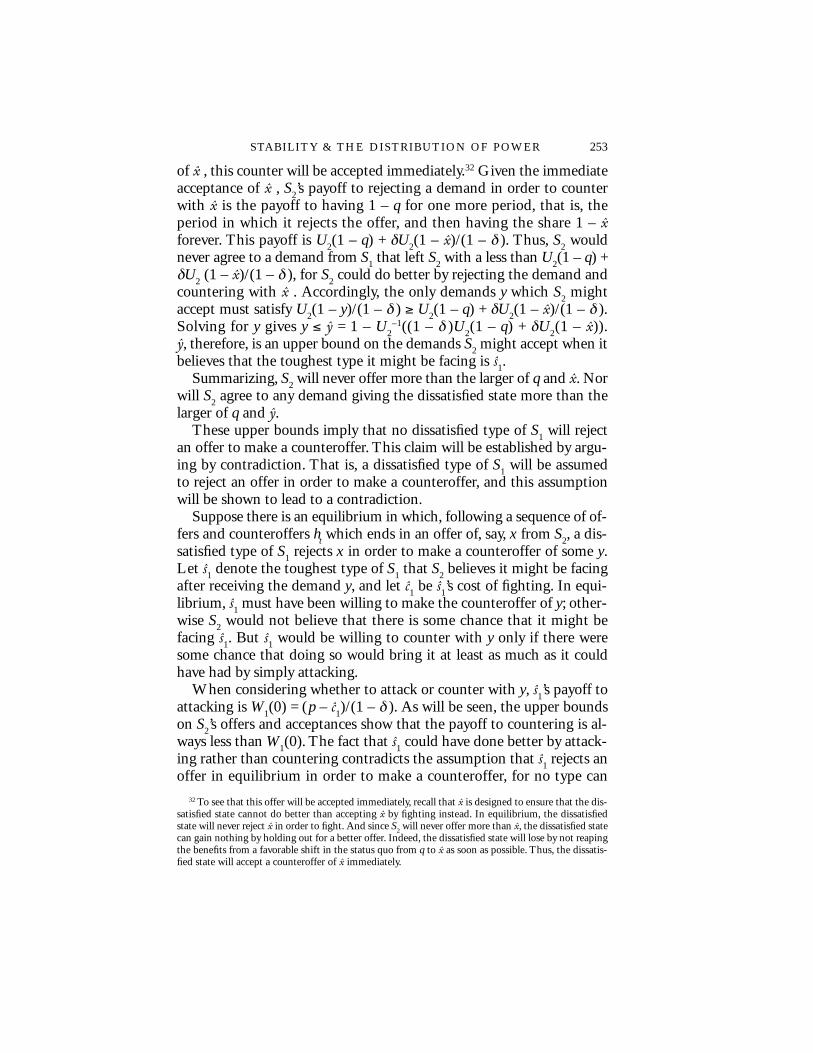
of x , this counter will be accepted immediately.32 Given the immediateacceptance of x , S2’s payoff to rejecting a demand in order to counterwith x is the payoff to having 1 – q for one more period, that is, theperiod in which it rejects the offer, and then having the share 1 – xforever. This payoff is U2(1 – q) + δU2(1 – x)/(1 – δ ). Thus, S2 wouldnever agree to a demand from S1 that left S2 with a less than U2(1 – q) +δU2 (1 – x)/(1 – δ ), for S2 could do better by rejecting the demand andcountering with x . Accordingly, the only demands y which S2 mightaccept must satisfy U2(1 – y)/(1 – δ ) ≥ U2(1 – q) + δU2(1 – x)/(1 – δ ).Solving for y gives y ≤ y = 1 – U2

–1((1 – δ )U2(1 – q) + δU2(1 – x)).y, therefore, is an upper bound on the demands S2 might accept when itbelieves that the toughest type it might be facing is s1.

Summarizing, S2 will never offer more than the larger of q and x. Norwill S2 agree to any demand giving the dissatisfied state more than thelarger of q and y.

These upper bounds imply that no dissatisfied type of S1 will rejectan offer to make a counteroffer. This claim will be established by argu-ing by contradiction. That is, a dissatisfied type of S1 will be assumedto reject an offer in order to make a counteroffer, and this assumptionwill be shown to lead to a contradiction.

Suppose there is an equilibrium in which, following a sequence of of-fers and counteroffers ht which ends in an offer of, say, x from S2, a dis-satisfied type of S1 rejects x in order to make a counteroffer of some y.Let s1 denote the toughest type of S1 that S2 believes it might be facingafter receiving the demand y, and let c1 be s1’s cost of fighting. In equi-librium, s1 must have been willing to make the counteroffer of y; other-wise S2 would not believe that there is some chance that it might befacing s1. But s1 would be willing to counter with y only if there weresome chance that doing so would bring it at least as much as it couldhave had by simply attacking.

When considering whether to attack or counter with y, s1’s payoff toattacking is W1(0) = (p – c1)/(1 – δ ). As will be seen, the upper boundson S2’s offers and acceptances show that the payoff to countering is al-ways less than W1(0). The fact that s1 could have done better by attack-ing rather than countering contradicts the assumption that s1 rejects anoffer in equilibrium in order to make a counteroffer, for no type can

32 To see that this offer will be accepted immediately, recall that x is designed to ensure that the dis-satisfied state cannot do better than accepting x by fighting instead. In equilibrium, the dissatisfiedstate will never reject x in order to fight. And since S2 will never offer more than x, the dissatisfied statecan gain nothing by holding out for a better offer. Indeed, the dissatisfied state will lose by not reapingthe benefits from a favorable shift in the status quo from q to x as soon as possible. Thus, the dissatis-fied state will accept a counteroffer of x immediately.


have a positive incentive to deviate from its equilibrium strategy. Thiscontradiction will establish the claim made in step 1.

If s1 rejects an offer to make a counteroffer, the game could end inonly one of three ways following the counter. First, the game could endin war in some future period. But the payoff to a dissatisfied type to liv-ing with the status quo for a while and then fighting is strictly less thanthe payoff to fighting now. In symbols, W1(t) < W1(0) for t ≥ 1. Thus, s1strictly prefers not to counter if the game is eventually going to end inwar.

The second way that the game could end is that s1 could ultimatelyaccept an offer from S2. But as shown above, S2 never offers more thanx . Consequently, s1’s maximum payoff to countering with y if the gamesubsequently ends with s1’s acceptance of an offer of x is s1’s payoff toliving with the status quo for two periods—namely, the period in whichs1 counters with y and then the period in which S2 rejects this offer inorder to counter with x—and then having x forever. In symbols, thispayoff is U1(q) + δU1(q) + δ 2U1(1 – x)/(1 – δ ). But this payoff is lessthan W1(0) = (p – c1)/(1 – δ ), because U1(x) = p – c1 and, since s1 is dis-satisfied, p – c1 > U1(q). Again, s1 does strictly better by fighting ratherthan countering if the game ends with s1’s ultimately accepting an offerfrom S2.

The final way that the game could end is with S2’s agreeing to a de-mand from s1. s1’s maximum payoff to this outcome occurs if s1 imme-diately counters with the maximal acceptable demand y and S2 accepts.This would leave s1 with the payoff to living with the status quo for theperiod in which it rejects x to counter with y and then having y forever.In symbols, s1’s payoff is U1(q) + δU1(y)/(1 – δ ). This payoff is strictlyless than s1’s payoff to fighting, ( p – c1)/(1 – δ ).33 As before, s1 doesstrictly better by fighting rather than countering if the game ends withS2 accepting s1’s demand.

In sum, s1 can increase its payoff by attacking rather than making acounteroffer regardless of how the game ends following s1’s counter.Accordingly, s1 would be able to increase its payoff by deviating from itsequilibrium strategy if its equilibrium strategy were to reject an offer inorder to make a counteroffer. This, however, is a contradiction becausethe definition of an equilibrium requires that no actor can improve its

33 To see that s1’s payoff is strictly less that W1(0) , note that the definition of y implies that S2 is in-different to accepting y now, which leaves S2 with 1 – y forever, and settling on x in the next period,which leaves S2 with 1 – x forever. Thus U2(1 – y)/(1 – δ ) = U2(1 – q) + δU2(1 – x)/(1 – δ) . But S2prefers the status quo share of 1 – q to what it will have after settling on either 1 – y or 1 – x. That is,1 – q > 1 – y . Given 1 – q > 1 – y, then the previous equality implies 1 – y > 1 – x or, equivalently, x > y.Finally, the fact that x > y > q leaves W1(0) = (p – c1)/(1 – δ) = U1(x)/(1 – δ) > U1(q) + δ U1(y)/(1 – δ).

254 WORLD POLITICS

payoff by deviating from its equilibrium strategy. This contradictionthus establishes the claim that no dissatisfied type can reject an offer inequilibrium in order to make a counteroffer. If, moreover, no dissatis-fied type will reject an offer to make a counter, then a dissatisfied typemust choose one of the two remaining alternatives. It will either acceptthe offer on the table or attack, depending on which alternative yieldsthe higher payoff.

Step 2. All satisfied types accept any offer larger than the status quo.

Assume as before that S1 is the potentially dissatisfied state and that thesatisfied state has offered to revise the status quo in favor of S1. Moreformally, S2 has offered S1 a share x where x > q . As shown in step 1, adissatisfied type of S1 rejects x if this type’s payoff to fighting is higherthan the payoff to accepting x and accepts x otherwise.

Now consider the decision facing a satisfied type of S1, which is de-noted by S1. S1 never attacks. To see that S1 does not attack, note that thepayoff to accepting x is greater than the payoff to living with the statusquo because x > q, and the payoff to living with the status quo is largerthan the payoff to fighting because S1 is satisfied. Thus, the payoff to ac-cepting x is greater than the payoff to fighting, and therefore S1 will notattack.

Given that S1 will not attack, its decision reduces to accepting x or re-jecting it in order to make a counteroffer. S1 will accept x because it of-fers the higher payoff. To calculate the payoff to rejecting x, recall thatno dissatisfied type of S1 will reject x in order to make a counteroffer. If,therefore, x is rejected, this rejection is in effect a signal to S2 that it isfacing only satisfied types of S1. But as soon as S2 becomes convincedthat it is facing only satisfied types of S1, it will find any threat from S1to use force to overturn the status quo inherently incredible. Thus, S2will never agree to revise the status quo in S1’s favor. The status quo,therefore, will not be revised following the rejection of x. Hence, S1’spayoff to rejecting x is the payoff to living with the status quo. But x >q, so the payoff to agreeing to x is higher than the payoff to living withthe status quo. Accordingly, satisfied types of the potentially dissatisfiedstate will accept any offer x > q.

To see what satisfied types do if S2 offers or, more aptly, demands arevision of the status quo in its favor, suppose x < q.34 As before, all dis-satisfied types of S1 will either accept x or fight, depending on which al-

34 The analysis of the case in which x = q is completely analogous.


ternative offers the higher payoff. Indeed, in the case in which S2 offersless than the status quo, all dissatisfied types fight. (By definition, alldissatisfied types prefer fighting to the status quo, and, with x < q, thepayoff to accepting x is even less than the payoff to the status quo.) Be-cause all dissatisfied types reject x and fight, S2 will infer once again thatit is facing only satisfied types of S1 if x is countered. And, as just seen,once S2 becomes convinced that it is facing only satisfied types, the sta-tus quo will not be changed. Thus, the choice confronting a satisfiedtype when x < q is to attack, accept the offer, or reject it and live withthe status quo. Of the three, a satisfied type prefers living with the sta-tus quo. The status quo payoff is higher than the payoff to accepting xbecause x < q and higher than the payoff to fighting because this type issatisfied. In sum, a satisfied type rejects x in equilibrium if x < q and itreceives the payoff to living with the status quo.

Step 3: Specifying the satisfied state’s optimal offers.

The first two steps in the derivation of the game’s equilibrium describehow the types of the potentially dissatisfied state respond to an offerfrom the satisfied state. The satisfied state, in turn, will make its bestoffer in light of these responses and its beliefs about the dissatisfiedstate’s costs. Let s2 denote the type of S2 with cost c2. Then given its be-liefs about the potentially dissatisfied state’s costs, s2 can determine theprobability that S1 will reject an offer of x and attack. (Assume for nowthat x > q.) To wit, the type of S1 with cost c1 will reject x and attack ifthis type is dissatisfied and prefers fighting to accepting x. In symbols,this type fights if p – c1 > U1(x) or, equivalently, p – U1(x) > c1 . But, S2’sbeliefs about S1’s costs can be used to calculate the probability that thiscost is less than p – U1(x) and therefore that an offer of x will lead towar. Let R(x) denote the probability that S1 will attack in response to x.

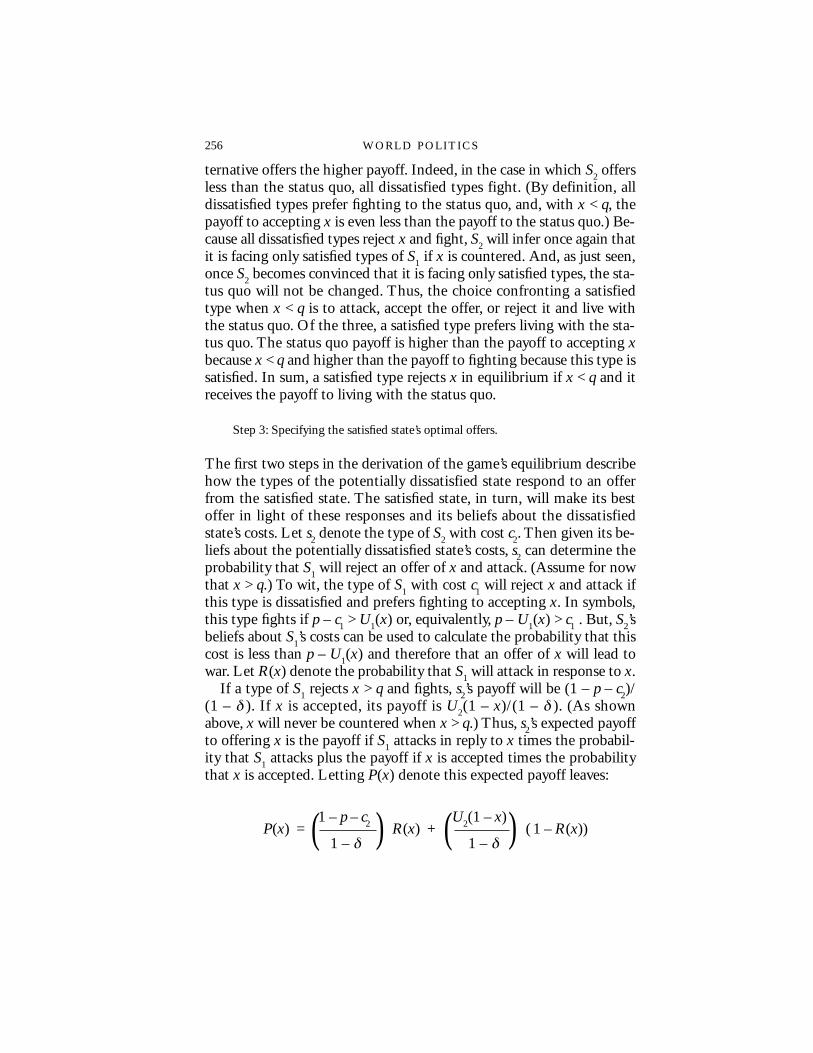
If a type of S1 rejects x > q and fights, s2’s payoff will be (1 – p – c2)/(1 – δ ). If x is accepted, its payoff is U2(1 – x)/(1 – δ ). (As shownabove, x will never be countered when x > q.) Thus, s2’s expected payoffto offering x is the payoff if S1 attacks in reply to x times the probabil-ity that S1 attacks plus the payoff if x is accepted times the probabilitythat x is accepted. Letting P(x) denote this expected payoff leaves:

256 WORLD POLITICS

P(x) = 1 – p – c2 R(x) +

U2(1 – x)( 1 – R(x))

1 – δ 1 – δ( ) ( )

s2, therefore, offers the value of x that maximizes P(x) subject to thecondition that x ≥ q.35

It is now straightforward to use the results of steps 1, 2, and 3 to de-scribe the unique perfect Bayesian equilibrium outcome of the bargain-ing game. Suppose that the game begins with the satisfied state’smaking the initial offer to the potentially dissatisfied state. The poten-tially dissatisfied state will respond to this initial offer as outlined above:dissatisfied types will accept it or fight, depending on which alternativeyields the higher payoff, and satisfied types will accept if the offer ismore than the status quo and will reject if it is less than the status quo.The satisfied state will then use its initial beliefs about the potentiallydissatisfied state’s costs to determine the probability that the potentiallydissatisfied state will respond to a particular offer by attacking. Andgiven these probabilities, the satisfied state will make its optimal offer,which is the value of x that maximizes P(x) for x ≥ q and where theprobability that an initial offer of x is rejected is R(x) = F1(p – U1(x)).36

The probability that the bargaining will end in war is, in equilibrium,simply the probability that the potentially dissatisfied state will reply tothis optimal initial offer by attacking.37

STABILITY AND THE DISTRIBUTION OF POWER

The equilibrium of the bargaining model makes it possible to calculatethe probability of war as a function of the distribution of power. Thissection calculates this relation in a specific case and then comparesthese results to the expectations of the balance-of-power and prepon-derance-of-power schools and to other formal work. The section alsooffers a possible explanation for the equivocal results of empirical ef-forts to determine the relation between stability and the distribution ofpower and briefly considers some of the difficulties of estimating thisrelation empirically. Finally, the section discusses the relation betweenthe probability of war and the distribution of power in more generalcases. As in the specific case analyzed in detail here, the expectations of

35 The expression for P(x) was derived on the basis of the assumption that x > q. If x ≤ q , s2’s ex-pected payoff to offering x is P(q). Accordingly, s2 is indifferent to offering any x ≤ q and it will sufficeto maximize P over the range x ≥ q .

36 s1 rejects x if p – c1 > U1(x) or p – U1(x) > c1 . Given that c1 is distributed according to the cumula-tive distribution function F1, the probability that c1 is less than p – U1(x) is F1(p – U1(x)).

37 Although cumbersome to show, the probability that the bargaining will end in war is essentiallythe same regardless of whether the satisfied state or the potentially dissatisfied state makes the initialoffer. See Powell (fn. 31) for the details.


both the balance-of-power and the preponderance-of-power schoolsfail to hold in these more general cases.

To simplify the analysis, assume that the states are risk neutral andthat each believes the other’s cost of fighting is uniformly distributedbetween zero and one. Risk neutrality and the previous normalizationsof the states’ utility functions imply that S1’s and S2’s utilities for the di-vision (x, 1 – x) are simply x and 1 – x, respectively.

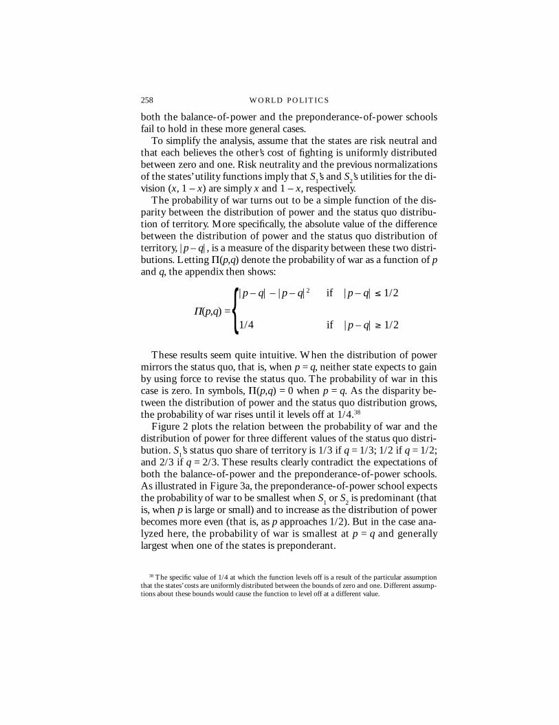
The probability of war turns out to be a simple function of the dis-parity between the distribution of power and the status quo distribu-tion of territory. More specifically, the absolute value of the differencebetween the distribution of power and the status quo distribution ofterritory, |p – q|, is a measure of the disparity between these two distri-butions. Letting Π(p,q) denote the probability of war as a function of pand q, the appendix then shows:

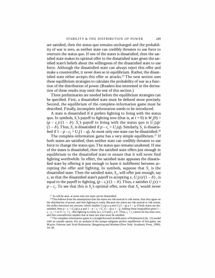
These results seem quite intuitive. When the distribution of powermirrors the status quo, that is, when p = q, neither state expects to gainby using force to revise the status quo. The probability of war in thiscase is zero. In symbols, Π(p,q) = 0 when p = q. As the disparity be-tween the distribution of power and the status quo distribution grows,the probability of war rises until it levels off at 1/4.38

Figure 2 plots the relation between the probability of war and thedistribution of power for three different values of the status quo distri-bution. S1’s status quo share of territory is 1/3 if q = 1/3; 1/2 if q = 1/2;and 2/3 if q = 2/3. These results clearly contradict the expectations ofboth the balance-of-power and the preponderance-of-power schools.As illustrated in Figure 3a, the preponderance-of-power school expectsthe probability of war to be smallest when S1 or S2 is predominant (thatis, when p is large or small) and to increase as the distribution of powerbecomes more even (that is, as p approaches 1/2). But in the case ana-lyzed here, the probability of war is smallest at p = q and generallylargest when one of the states is preponderant.

38 The specific value of 1/4 at which the function levels off is a result of the particular assumptionthat the states’ costs are uniformly distributed between the bounds of zero and one. Different assump-tions about these bounds would cause the function to level off at a different value.

258 WORLD POLITICS

|p – q| – |p – q|2 if |p – q| ≤ 1/2

Π(p,q) =1/4 if |p – q| ≥ 1/2{

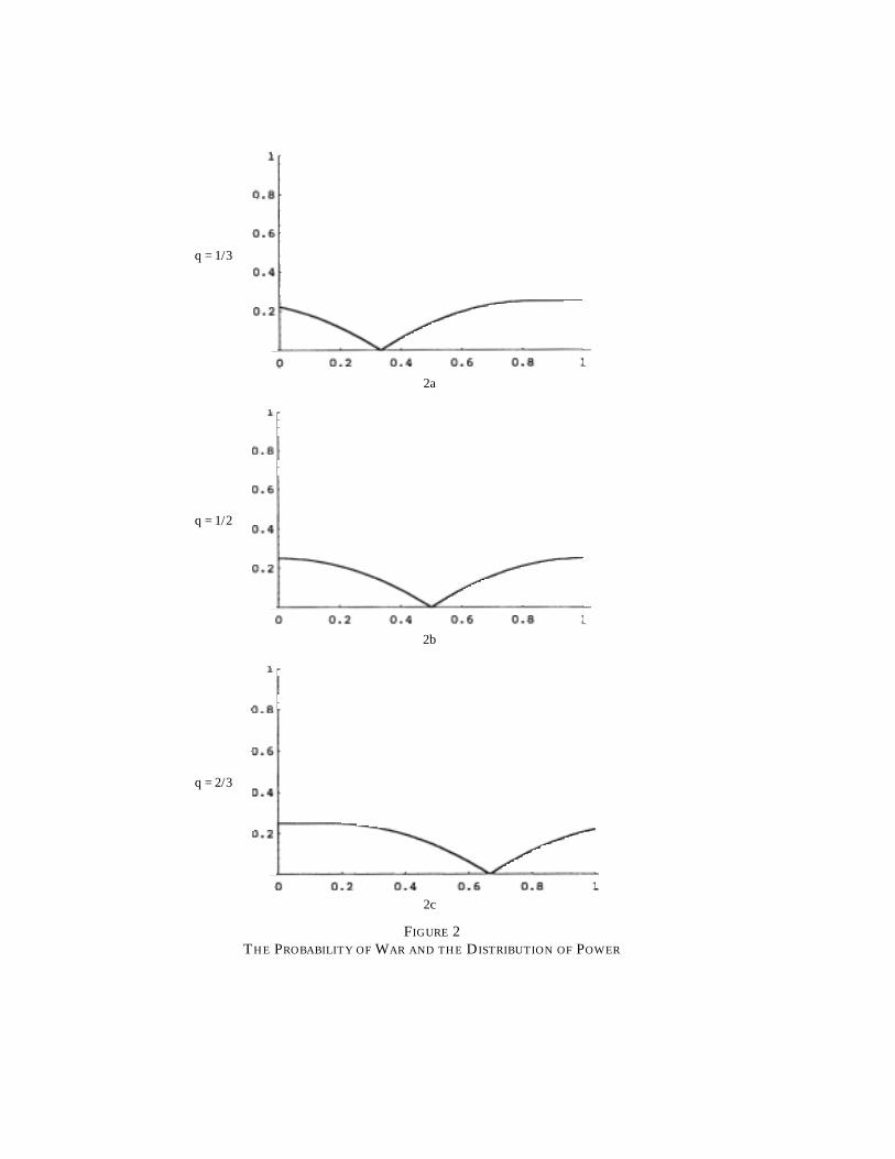
FIGURE 2THE PROBABILITY OF WAR AND THE DISTRIBUTION OF POWER

q = 1/3

q = 1/2

q = 2/3

2a

2c

2b

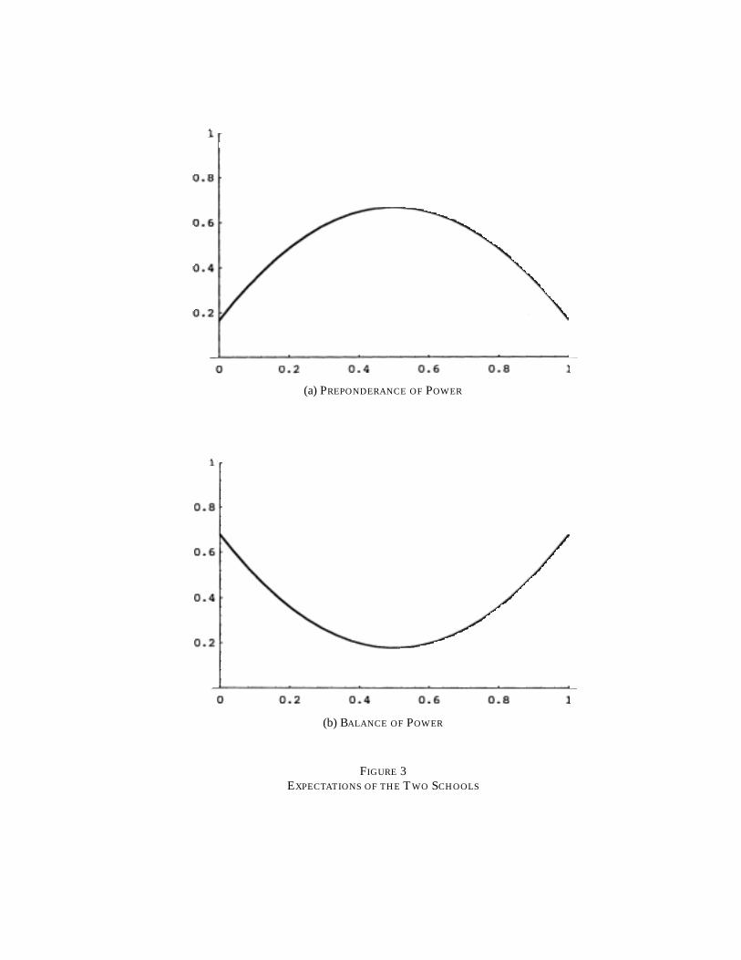
(a) PREPONDERANCE OF POWER

(b) BALANCE OF POWER

FIGURE 3EXPECTATIONS OF THE TWO SCHOOLS

Figure 3b illustrates the balance-of-power school’s expectations. Theprobability of war is smallest when there is a roughly even distributionof power (p is approximately 1/2) and increases as the distribution ofpower becomes skewed. These expectations correspond to the formalresults only in the special circumstance in which the status quo divisionis even (q = 1/2). When the status quo division is uneven, as in Figure2a and 2c, the probability of war in the model is smallest when the dis-tribution of power mirrors the uneven status quo division and not, asthe balance-of-power school asserts, when the distribution is even.

The present analysis also complements and qualifies the results ofother formal analyses of the relation between stability and the distribu-tion of power. Bueno de Mesquita and Lalman, for example, study amodel in which two states bargain about revising the status quo.39 Intheir game each state has the opportunity to make a single demand ofthe other state. After both states have made their demands, each statedecides whether or not to use force to secure its demand. In one ver-sion of this game Bueno de Mesquita and Lalman assume that the sizeof each state’s demand is determined outside the model. That is, theamount each state demands is simply one of the exogenously specifiedinitial conditions of the model. In this version of Bueno de Mesquitaand Lalman’s model, the size of a state’s demand is not determined aspart of a state’s equilibrium strategy. A state does not determine howmuch it demands by balancing the risk of war against the chance ofagreeing on a more favorable settlement. The justification for assumingthe states’ demands to be exogenous is that these demands are “deter-mined by internal political rules, procedures, norms, and considerationsand may or may not be attuned to foreign policy considerations.’’40

With the size of the states’ demands determined outside the model,Bueno de Mesquita and Lalman find that “dissatisfaction with the sta-tus quo is entirely unrelated to the likelihood of war.’’41

The present analysis focuses specifically on how a state balances thegreater risk that a larger demand will lead to war against the higherpayoff the state will obtain if this larger demand is accepted. This focusrequires a model in which the states determine the sizes of their de-

39 Bueno de Mesquita and Lalman (fn. 2, 1992).40 Ibid., 41.41 Ibid., 190. In a second version of their game, Bueno de Mesquita and Lalman let the state’s de-

mands be determined as part of their equilibrium strategies. But this game has complete information.The combination of endogenous demands and complete information means that the probability of waris zero in their model—as well as in the model analyzed above—regardless of the distribution ofpower. Bueno de Mesquita and Lalman do not examine the case in which there are both endogenousdemands and incomplete information.


mands as part of their equilibrium strategies. The game examined heresatisfies this requirement. The probability of war in the present game,unlike in Bueno de Mesquita and Lalman’s model, is closely related tothe level of dissatisfaction with the status quo.42 The larger the level ofdissatisfaction in the case above, that is, the larger the disparity |p – q|,the more likely war.43

Fearon also considers the relation between the probability of war andthe distribution of power. He studies a game in which one state makesa take-it-or-leave-it offer after which a second state must then eitheraccept this offer or attack. By assumption, this second state cannotmake a counteroffer. The size of the state’s demand in Fearon’s model isdetermined as part of the state’s equilibrium strategy, and he finds thatthe probability of war is “completely insensitive’’ to the distribution ofpower.44

The current model complements Fearon’s formulation. He is study-ing a stylized situation in which one state presents another state withan ultimatum in the form of a military fait accompli. This fait accompliestablishes a new distribution that will become the new internationalstatus quo unless the second state goes to war to reverse it.45 In the styl-ized situation modeled in this essay, two states are bargaining about re-vising the status quo and have the opportunity to make offers andcounteroffers. There are, however, no military faits accomplis: any useof force to revise the status quo is assumed to lead directly to war. Inthese circumstances the probability of war is sensitive to the distribu-tion of power and, in particular, to the disparity between the distribu-tion of power and the status quo distribution of territory.

The present analysis provides a possible explanation of the equivocalfindings of empirical efforts to determine the relation between stabilityand the distribution of power. Empirical research has yielded at leastthree different findings about an even distribution: that it is more stablethan a preponderance of power,46 that it is less stable than a preponder-ance of power,47 and, depending on whether one looked at the nine-teenth or the twentieth century, that it is either more or less stable.48

42 Bueno de Mesquita and Lalman (fn. 2, 1992), 190.43 Strictly speaking, the probability of war increases as |p – q| increases only as long as |p – q| < 1/2.

After this, the probability of war levels off.44 Fearon (fn. 4), 20.45 Ibid., 15.46 Siverson and Tennefoss (fn. 2).47 Kim (fn. 2, 1992); and Moul (fn. 2).48 Singer, Bremer, and Stuckey (fn. 2).

262 WORLD POLITICS

Other work has found no significant relation between stability and thedistribution of power.49

The equilibrium of the bargaining game shows that the probabilityof war depends on both the distribution of power and the status quodistribution. Thus, any attempt to assess the relation between the prob-ability of war and the distribution of power should control for the sta-tus quo. Failing to do so will generally lead to biased estimates if, asmight be expected, the distribution of power and the status quo distri-bution are correlated. But empirical efforts to estimate this relationhave generally not controlled for the status quo, and this omission maypartially account for the equivocal empirical results.50

Finally, it is important to ask about the generality of these results. Dothe findings hold only in the specific example considered here in whichthe states were assumed to be risk neutral and to believe that eachother’s cost or willingness to use force was uniformly distributed? Or dothe results also hold in more general conditions? The central findingthat the probability of war is at a minimum when the distribution ofpower mirrors the status quo distribution is quite robust. It holds aslong as the states are risk neutral or risk averse, regardless of the partic-ular shapes of their utility functions or of the particular shapes of theprobability distributions representing their beliefs.51 Thus, the modelcontradicts the expectations of the balance-of-power and prepon-derance-of-power schools as long as the states are risk neutral or riskaverse.52

One might also wonder if this result holds if the uncertainty sur-

49 Maoz (fn. 2); and Bueno de Mesquita and Lalman (fn. 2, 1992).50 Unfortunately, the theoretical results derived here, while indicating the importance of controlling

for the status quo, do not identify a means of doing so. The basic problem is to find a way of measur-ing a state’s utility for the status quo. Bueno de Mesquita and Lalman’s (fn. 2, 1992) measure of thisutility may offer a start in this direction, but their current formulation is inadequate. If the states arerisk neutral as in the example above, then Bueno de Mesquita and Lalman’s measure reduces to as-suming that the status quo distribution is constant in all cases. In terms of the example above, they arein effect assuming that q always equals 1/2. (To obtain q = 1/2, assume the state is risk neutral by tak-ing rA = 1 in equation A1.3 in Bueno de Mesquita and Lalman (fn. 2, 1992), 294, and normalize thestate’s utility to be one if it obtains everything it demands and zero if the other state obtains every-thing it demands by setting UA(∆A ) = 1 and UA(∆B ) = 0 .) Controlling for the status quo, however, re-quires the status quo to be treated as a variable across cases, and it is unclear how to do this with theirmeasure as it is currently formulated.

51 To see this, suppose that the distribution of power closely mirrors the status quo distribution ofterritory in that |p – q| is less than the minimium of the lowest possible costs of fighting, i.e., the min-imum of c1 and c2. Then, p – q ≤ c1 and q – p ≤ c2. These inequalities and the concavity of U1 and U2imply p – c1 ≤ q ≤ U1(q) and 1 – p – c2 ≤ 1 – q ≤ U2(1 – q). Thus, both S1 and S2 are satisfied, and theprobability of war is zero.

52 The case of risk-acceptant states introduces nonconvexities and technical difficulties, and theanalysis of this case remains a task for future work.


rounding the states’ willingness to use force varies with shifts in the dis-tribution of power. More specifically, the costs of fighting in the exam-ple examined here are always uniformly distributed between 0 and 1regardless of the distribution of power. But what would happen if theexpected cost and uncertainty about a state’s willingness to use force de-clined as that state became more powerful?53

This question requires a two-part response. First, the question itselftakes the analysis beyond the balance-of-power and predominance-of-power schools, as neither school bases its argument on the subtletiesimplicit in this question. Second, the model provides a partial answerto this question. The probability of war is still zero as long as the statusquo distribution of benefits mirrors the distribution of power.54 Onceagain, the expectations of the balance-of-power and preponderance-of-power schools fail to hold.55

CONCLUSION

The relation between the distribution of power and the probability of war is an important and long-debated problem in international relations theory. The balance-of-power school argues that an even dis-tribution of power brings greater stability, while the preponderance-of-power school argues that a preponderance brings greater stability.These opposing claims have been examined in the context of an infi-nite-horizon bargaining game in which two states alternate making of-fers about how to revise the international status quo. The bargainingcontinues until the states agree on a revision or until one of them be-comes sufficiently pessimistic about the prospects of reaching a mutu-ally agreeable settlement that it resorts to force in an attempt to imposea new settlement. Contradicting the expectations of both the balance-of-power and preponderance-of-power schools, the probability of warin the model is smallest when the distribution of power mirrors the sta-tus quo distribution.

53 More formally, suppose that the distributions of cost F1 and F2 were also a function of p and thatthe mean and variance of F1 decrease in p while the mean and variance of F2 decrease in 1 – p.

54 Even if F1 and F2 depend on p, the argument in footnote 26 goes through with only minor mod-ification.

55 The model’s answer is only partial because the shape of the function relating the probability ofwar to the distribution of power, while always zero when p = q, is likely to depend on the states’ utilityfunctions and on the functional forms of the probability distributions representing their beliefs.

264 WORLD POLITICS

APPENDIX

There are two cases to consider in calculating the probability of war asa function of the distribution of power. Suppose, first, that p > q. ThenS1 is the potentially dissatisfied state, because the expected payoff tofighting for the type of S1 with the lowest cost of fighting is strictlygreater than its status quo payoff: p – c1 = p – 0 > q. Then, as shownabove, the probability of war in the bargaining game is the probabilitythat the dissatisfied state attacks in response to the satisfied state’s op-timal initial offer.

To calculate this probability, S2’s optimal initial offer must first bedetermined. Suppose S2 offers x to S1. A dissatisfied type s1 of S1 withcost c1 will reject this offer and attack if its payoff to fighting is higherthan its payoff to accepting. That is, s1 attacks if p – c1 > x or, equiva-lently, if p – x > c1. Thus, the probability that S1 will attack in responseto an offer of x is the probability that S1’s cost is less than p – x. Giventhat S1’s costs of fighting are uniformly distributed between 0 and 1, theprobability that S1’s cost is less than p – x is just p – x. Consequently, S2’sexpected payoff to offering x, which will be denoted by P (x), is its pay-off to fighting times the probability that S1 will attack plus the payoff ifS1 accepts x times the probability that S1 will accept x. In symbols,

if S2’s offer is between q and p. If S2 offers more than p, then even thedissatisfied state with the lowest cost of fighting will prefer to acceptthe offer to fighting. Consequently, the probability that an offer of x > pwill be rejected is 0. S2’s payoff to offering x in this case reduces to (1 – x)/(1 – δ). If S2 offers x < q, then all dissatisfied types fight and all othertypes reject the demand which leave the status quo unchanged. S2’s pay-off is:

S2’s optimal offer is the value of x that maximizes its expected payoff.To describe the solution to this maximization problem, set the deriva-tive of P(x) equal to zero and let x*(c2) denote the solution to this equa-


P(x) = 1 – p – c2 (p – x) +

(1 – x)( 1 – (p – x))

1 – δ 1 – δ

1 – p – c2 (p – q) + (1 – q)

( 1 – (p – q)).1 – δ 1 – δ

tion. This leaves x*1(c2) = p – (1 – c2)/2. Then the optimal offer of thetype of S2 with cost c2 is x*(c2) as long as x*(c2) ≥ q . S2’s optimal offer isq if x*(c2) < q.

Now that the equilibrium offers have been specified, the probabilityof breakdown can be calculated. Let π(c2) be the probability that thetype of S2 with cost c2 will be attacked. If x*(c2) < q for this type, thenthis type will offer q. The probability that the dissatisfied state will at-tack in response to this offer is the probability that the cost of fightingc1 is less than p – q which, given the uniform distribution of costs, issimply p – q. Thus, π(c2) = p – q for all types of S2 for which x*(c2) < q or,equivalently, for all types of S2 for which c2 < 1 – 2(p – q) .

If x*(c2) ≥ q for a type of S2, then this type will offer x*(c2). The prob-ability that the dissatisfied state attacks in response to this offer is p – x*(c2) = p – (p – (1 – c2)/2) = (1 – c2)/2. Thus, π(c2) = (1 – c2)/2 wheneverx*(c2) ≥ q or c2 ≥ 1 – 2(p – q) .π(c2) specifies the probability that the particular type of S2 with cost c2

will fight. But from the perspective of an outside observer, as well asfrom that of S1, S2’s cost is uncertain. Thus the probability of war is theexpected value of π(c2) . Letting Π(p,q) denote this expected value, then:

Π(p, q) describes the relation between the probability of breakdownand the distribution of power if p > q and, consequently, S1 is the dis-satisfied state. If p < q, then S2 is the dissatisfied state and the relationbetween stability and the probability of war must be determined anew.Fortunately, the symmetry of the problem makes it easy to find this re-lation in this second case. Let p' = 1 – p and q' = 1 – q . Then p < q im-plies p' > q' . Moreover, p' now measures the probability that the dis-satisfied state will prevail and q' measures the dissatisfied state’s statusquo payoff just as p and q did in the first case where p > q . The symme-try of the example then ensures that the probability of breakdown if p <

266 WORLD POLITICS

(p – q) – (p – q)2 if 0 ≤ p – q ≤ 1/2

Π(p,q) =1/4 if 1/2 ≤ p – q{

1Π(p,q) = π(c2)dc2

0∫

q is given by Π(p', q' ). But Π(p', q' ) is just Π(1 – p, 1 – q) which in turnequals (q – p)(1 – (q – p)) if 1 – 2(q – p) ≥ 0 and 1 /4 if 1 – 2(p – q) < 0.

Combining these results leaves:


|p – q| – (p – q)2 if |p – q| ≤ 1/2

Π(p, q) =1/4 if |p – q| ≥ 1/2{

Documents

STABILITY AND THE DISTRIBUTION OF POWER 1996.pdf · World Politics 48 (January 1996), 239–67 STABILITY AND THE DISTRIBUTION OF POWER By ROBERT POWELL* THE relation between the distribution