Stability analysis and synthesis of hybridclosed-loops for modern power systems

Sums Of Squares for Lyapunov Stability

Matteo TacchiEnd-of-study Engineer Internship

15 of September 2016 - 28 of February 2017

CHAIRE INTERNATIONALE AUTOMATIQUE ET RESEAUXELECTRIQUES

Supervisors :Bogdan MarinescuHead of the RTE - ECN IndustrialChair

Marian AnghelResearcher at Los Alamos National

Laboratory

Contents

Contents i

List of figures ii

Introduction 1

1 Context 21.1 RTE and its industrial chair . . . . . . . . . . . . . . . . . . . . . . . . . . . . . . 21.2 LS2N (former IRCCyN) . . . . . . . . . . . . . . . . . . . . . . . . . . . . . . . . 3

2 Preliminaries : Sums of Squares and Lyapunov stability 42.1 Lyapunov stability . . . . . . . . . . . . . . . . . . . . . . . . . . . . . . . . . . . 4

2.1.1 Notions of stability and positive definiteness . . . . . . . . . . . . . . . . . 42.1.2 Stability theorems . . . . . . . . . . . . . . . . . . . . . . . . . . . . . . . 5

2.2 Sums of Squares . . . . . . . . . . . . . . . . . . . . . . . . . . . . . . . . . . . . 62.2.1 General results . . . . . . . . . . . . . . . . . . . . . . . . . . . . . . . . . 62.2.2 The Positivstellensatz . . . . . . . . . . . . . . . . . . . . . . . . . . . . . 92.2.3 Application to Lyapunov stability analysis . . . . . . . . . . . . . . . . . . 102.2.4 The Expanding Interior problem . . . . . . . . . . . . . . . . . . . . . . . 12

3 The Model 153.1 Nominal Operating Equations . . . . . . . . . . . . . . . . . . . . . . . . . . . . . 15

3.1.1 Writing the equations . . . . . . . . . . . . . . . . . . . . . . . . . . . . . 153.1.2 Validation of the nominal system . . . . . . . . . . . . . . . . . . . . . . . 17

3.2 The Short-Circuit Model . . . . . . . . . . . . . . . . . . . . . . . . . . . . . . . . 193.2.1 Writing the short-circuit equations . . . . . . . . . . . . . . . . . . . . . . 193.2.2 Simulation of the short-circuited system . . . . . . . . . . . . . . . . . . . 23

4 Lyapunov Stability Analysis 254.1 Writing the equations under the state space form . . . . . . . . . . . . . . . . . . 25

4.1.1 The “physical” state variables . . . . . . . . . . . . . . . . . . . . . . . . . 254.1.2 Shift to equilibrium point . . . . . . . . . . . . . . . . . . . . . . . . . . . 274.1.3 Recasting the equations into a polynomial system . . . . . . . . . . . . . 284.1.4 A Lie-Blacklund transformation . . . . . . . . . . . . . . . . . . . . . . . . 30

4.2 Estimating the R.O.A. using SOSTOOLS . . . . . . . . . . . . . . . . . . . . . . 334.2.1 Statement of the problem and structure of the codes . . . . . . . . . . . . 334.2.2 A first (im)practical implementation . . . . . . . . . . . . . . . . . . . . . 344.2.3 An intermediate step : tackling a simplified model . . . . . . . . . . . . . 364.2.4 Intrepretation of the results . . . . . . . . . . . . . . . . . . . . . . . . . . 39

5 Personal work and contributions 42

Conclusion 43

i

List of Figures

2.2.1 The expanding D algorithm . . . . . . . . . . . . . . . . . . . . . . . . . . . . . . 122.2.2 The expanding interior algorithm . . . . . . . . . . . . . . . . . . . . . . . . . . . 143.1.1 Synchronous machine connected to an infinite bus . . . . . . . . . . . . . . . . . 153.1.2 The equivalent simplified system . . . . . . . . . . . . . . . . . . . . . . . . . . . 153.1.3 Simulation of the state variables for the nominal system . . . . . . . . . . . . . . 173.1.4 Simulation of the nominal system with perturbations . . . . . . . . . . . . . . . . 183.2.1 The short-circuited system . . . . . . . . . . . . . . . . . . . . . . . . . . . . . . . 193.2.2 Our first short-circuit model . . . . . . . . . . . . . . . . . . . . . . . . . . . . . . 203.2.3 Representation of VG . . . . . . . . . . . . . . . . . . . . . . . . . . . . . . . . . . 203.2.4 Representation of Zeq . . . . . . . . . . . . . . . . . . . . . . . . . . . . . . . . . 213.2.5 Representation of Veq . . . . . . . . . . . . . . . . . . . . . . . . . . . . . . . . . 213.2.6 The current injection method . . . . . . . . . . . . . . . . . . . . . . . . . . . . . 223.2.7 Simulation of the state variables for tc = 350s and tcl = 350.144s . . . . . . . . . 243.2.8 Simulation of the state variables for tc = 350s and tcl = 350.145s . . . . . . . . . 254.2.1 Structure of initV (left) and asstabI (right) . . . . . . . . . . . . . . . . . . . . 354.2.2 Simulation of the state variables for the simplified system and tc = 350s and

tcl = 354.057s . . . . . . . . . . . . . . . . . . . . . . . . . . . . . . . . . . . . . . 374.2.3 Simulation of the state variables for the simplified system and tc = 350s and

tcl = 354.058s . . . . . . . . . . . . . . . . . . . . . . . . . . . . . . . . . . . . . . 384.2.4 Simulation of the Lyapunov function V for tc = 10s (top : ∆t = 4.057s ; bottom

: ∆t = 4.058s) . . . . . . . . . . . . . . . . . . . . . . . . . . . . . . . . . . . . . 394.2.5 Cuts of the R.O.A. estimate in the planes (δ, ω), (e′q, Efd) and (Pm, ω) . . . . . . 404.2.6 Top : ωinit = ωref + 0.211pu ; bottom : ωinit = ωref + 0.212pu . . . . . . . . . . 41

ii

Introduction : the problem of power grids stability

In the wake of the Energy Transition, and with the help of the European Union, the sector ofelectricity transportation is in a phase of huge changes to adapt to new technology challenges.Indeed, the increasing part of renewables in French and European energy production raises newstability issues, since stability of the power grids is currently under the responsibility of thenuclear sector. Apart from stability, the multiplication of offshore wind power sources asks for abetterment in the technologies of HVDC lines, for example.

There are many notions of stability in power systems. In this work we will focus on transientstability, as defined in [1]

Definition 0.1. Transient Stability denotes the ability of a power system to return to operatingequilibrium after a large disturbance, and within a short amount of time (under 10s), usuallygoing through a first-swing aperiodic drift.

For this internship, the problem we adress is the one of a synchronous machine linked toan infinite bus through lines in which a short-circuit occurs. The short circuit induces a largedisturbance which has to be eliminated in a matter of milliseconds : this is a transient stabilityanalysis.

The mathematical approach resorts to Lyapunov functions, which has been unusual for powersystems since until now it could not be applied to resistive systems (with non-zero resistances,i.e. basically all the real systems), and proved very sensitive to the number of variables and thecomplexity of the power grid (see e.g. [2]).

However, the use of the Sums Of Squares theory greatly facilitates the research of a suitableLyapunov function, providing large estimates of the equilibrium points’ regions of attraction, aswe are going to show in this report. This was first investigated in [3], and proved more efficientthan energy methods presented before in [2], in the simple case of a non-regulated multi-machinepower system.

The aim of this internship is to extend the work presented in [3] to power systems thatinclude regulations towards frequency, voltage and mechanical power. Such systems are morecomplicated than the former : they introduce new variables and dynamics that are sometimeshard to study.

1

1 Context

1.1 RTE and its industrial chair

RTE (Electricity Transport Networks) is an affiliate company of EDF1. It is in charge of thetransportation of electricity through the country, the maintenance of the network, the electricityimport-export, the supply of electricity for industrial companies such as SNCF2 and the integra-tion of new energy producers in the electricity marcket. RTE is the owner of the largest powergrid in all Europe, with over 100 000 km of high voltage lines and 2 600 electrical facilities. Itreaches over 100 GW of consumption during the peaks. The company makes e4 702 millionsand invests e1 447 millions each year. (see e.g. [4])

Its missions are :

• Mainteining and developing the power grid so as to connect electricity producers, distrib-utors and consumers, facilitate energy exchanges through Europe and secure the facilities

• Exploiting the network safely, with special attention to the technical constraints on it,assuring the balance between production and consumption and a fair access to the powergrid

• optimizing the economical and ecological costs of the electricity transport

RTE has four (4) major ambitions : integrating renewable power sources to the network, en-couraging a more flexible consumption, developping the network facilities and invest in computerscience and smart grids.

RTE has an R&D - Innovation branch which is in charge of three general objectives :

• Anticipating the evolution of the electrical system so as to design efficient and sustainablesolutions, to adapt the technologies to the evolutions of the context (environment, marcket,politics) and benefit from scientific breakthroughs

• Preparing the evolution of the jobs and the company for the future by creating softwares,methods and tools, orienting and integrating technological innovations

• Promoting and organising innovation within RTE

The RTE chair is an international industrial chair based on automatics and power networks,which aims to facilitate the energy transition through the use of smart grids and the integrationof renewable power sources into the European power network.

The chair combines resources from RTE and the Ecole Centrale Nantes, a French engineerschool which has been a leader in the sector of automatics for over 30 years. This way, RTE isable to prepare skilled engineers so as to work efficiently on the challenges of the future, especiallyfor energy transition and technologic innovation.

The RTE chair works in collaboration with the IRCCyN3 and the GeM4, two laboratoriesintegrated in the Ecole Centrale Nantes and recognized by the CNRS5. By combining Researchand Higher Education, the RTE chair intends to be a leader in the sector of energy technology

1. French Electricity Distribution, the French electricity distribution firm which owns the production of elec-tricity and sells it to civilians, and is the main responsible of French power sources.

2. French National Railway Society, a state company which manages the French railway.3. Nantes’ Research Institute in Communication and Cybernetics.4. Research Institute in Civil and Mechanical engineering5. French National Scientific Research Centre, the main state research organisation in France, which leads the

public research and laboratories.

2

and smart grids, by designing new tools for simulation, analysis and control, and by creatinga dynamic skill pool within the Ecole Centrale Nantes so as to encourage the development ofsmart grids.

Especially, in the domain of Control / Analysis / Decision : the progression of energy tran-sition leads to a more and more complex power network, with the integration of decentralisedand time-dependent power sources, HVDC6 and power electronics converters, which have a farreaching impact on the dynamics of the power grid.

Thus, it is necessary to design new control tools so as to manage the network in a reactiveand coordinated manner. This implies a more systemised use of nonlinear tools to analysethe impact of HVDC lines on the dynamics (and stability) of the power system (inter-zoneoscillations, transient stability in neighbour zones) and to design new robust control solutions(see e.g. [5]).

1.2 LS2N (former IRCCyN)

IRCCyN was the former name of the Research Institute in Communications and Cybernetics ofNantes (see e.g. [6]). It is a laboratory which has facilities in the Ecole Centrale Nantes, theEcole des Mines of Nantes, PolytechNantes and the IUT (University Institute of Technology) ofNantes. The main building is located in the Ecole Centrale Nantes.

IRCCyN is a Mixed Research Unit (UMR) of the CNRS. It is connected to INS2I, INSIS andINSB7, and works under the tutelage of Ecole Centrale Nantes, Nantes University and Ecole desMines of Nantes.

IRCCyN is a member of two research federations : AtlanSTIC (research federation in Sci-ence and Technologies for Information and Communication) and IRSTV (Research Institute ofSciences and Technics for the City), which are both recognized by the CNRS.

In January 2013, the IRCCyN was composed of 98 professors and researchers, 18 engineers,technicians and administratives, 105 PhD. students, 6 post-docs and 18 other employees. Therewere also 5 associate members and 10 special collaborators.

IRCCyN is involved in the production of new academic knowledge, as well as innovativemethods and tools designed as solutions to real problems posed by industrial firms and servicescompanies. The research spectrum covered by the IRCCyN is very large and includes automat-ics, image and signal processing, robotics, conception, modeling and optimisation of productionprocesses, virtual engineering, on-board systems, bio-informatics, cognitive psychology and er-gonomy.

IRCCyN is involved in corporate partnerships as well as national projects and internationalcooperation (especially with Mexico, Czech Republic, China, Korea, Poland, Italy, South Africa,Malaysia, USA, Russia and Spain). It is associated with three PhD Schools :

• Nantes University’s STIM (Science and Technology of Information and Mathematics)

• Ecole Centrale Nantes’ SPIGA (Science For Engineer, Geoscience and Architecture)

• Rennes University’s SHS (Humanities and Social Science)

In January 2017, the IRCCyN was fused with the LINA8 into the LS2N9, which gathers both

6. high voltage direct current lines, which are used to connect countries with one another7. Institute of Information Sciences and their Interactions, Institute of Engineering and System Sciences and

Institute in Biological Sciences8. Atlantic Nantes’ Laboratory of Computer Science, another UMR9. Laboratory of Digital Science of Nantes

3

laboratories. Consequently I was first hosted by the IRCCyN from September to December of2016 and then by the LS2N in January and February 2017.

The RTE chair links RTE and Ecole Centrale Nantes. However, the chair is located in theLS2N offices, in Ecole Centrale Nantes. As a consequence, i spent most of my time in thislaboratory, and worked and exchanged with some of its members.

2 Preliminaries : Sums of Squares and Lyapunov stability

2.1 Lyapunov stability

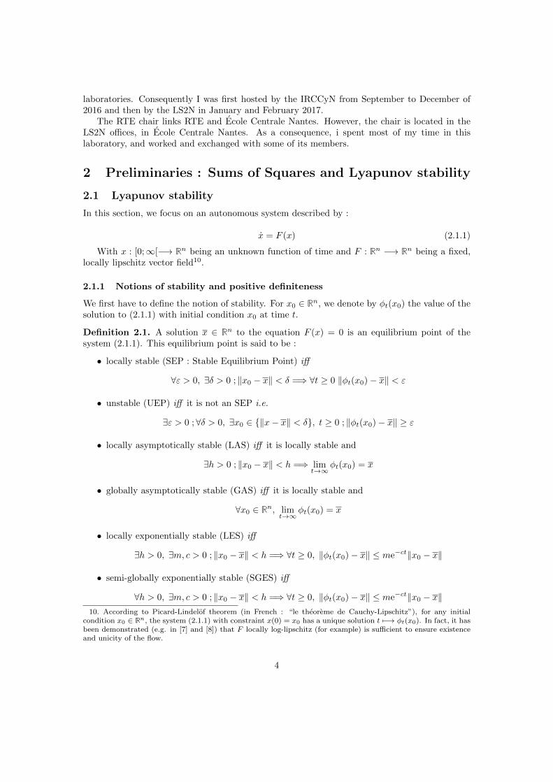
In this section, we focus on an autonomous system described by :

x = F (x) (2.1.1)

With x : [0;∞[−→ Rn being an unknown function of time and F : Rn −→ Rn being a fixed,locally lipschitz vector field10.

2.1.1 Notions of stability and positive definiteness

We first have to define the notion of stability. For x0 ∈ Rn, we denote by φt(x0) the value of thesolution to (2.1.1) with initial condition x0 at time t.

Definition 2.1. A solution x ∈ Rn to the equation F (x) = 0 is an equilibrium point of thesystem (2.1.1). This equilibrium point is said to be :

• locally stable (SEP : Stable Equilibrium Point) iff

∀ε > 0, ∃δ > 0 ; ‖x0 − x‖ < δ =⇒ ∀t ≥ 0 ‖φt(x0)− x‖ < ε

• unstable (UEP) iff it is not an SEP i.e.

∃ε > 0 ;∀δ > 0, ∃x0 ∈ ‖x− x‖ < δ, t ≥ 0 ; ‖φt(x0)− x‖ ≥ ε

• locally asymptotically stable (LAS) iff it is locally stable and

∃h > 0 ; ‖x0 − x‖ < h =⇒ limt→∞

φt(x0) = x

• globally asymptotically stable (GAS) iff it is locally stable and

∀x0 ∈ Rn, limt→∞

φt(x0) = x

• locally exponentially stable (LES) iff

∃h > 0, ∃m, c > 0 ; ‖x0 − x‖ < h =⇒ ∀t ≥ 0, ‖φt(x0)− x‖ ≤ me−ct‖x0 − x‖

• semi-globally exponentially stable (SGES) iff

∀h > 0, ∃m, c > 0 ; ‖x0 − x‖ < h =⇒ ∀t ≥ 0, ‖φt(x0)− x‖ ≤ me−ct‖x0 − x‖10. According to Picard-Lindelof theorem (in French : “le theoreme de Cauchy-Lipschitz”), for any initial

condition x0 ∈ Rn, the system (2.1.1) with constraint x(0) = x0 has a unique solution t 7−→ φt(x0). In fact, it hasbeen demonstrated (e.g. in [7] and [8]) that F locally log-lipschitz (for example) is sufficient to ensure existenceand unicity of the flow.

4

• globally exponentially stable (GES) iff

∃m, c > 0 ;∀x0 ∈ Rn, ∀t ≥ 0, ‖φt(x0)− x‖ ≤ me−ct‖x0 − x‖

In case of exponential stability, c is called the convergence rate.

The main result about stability is due to Lyapunov. It uses the notion of positive definitefunctions :

Definition 2.2. Let Ω ⊆ Rn be an open set containing 0 and ρ : Ω −→ R be a continuous scalarfunction. We will say that ρ is :

• positive semi-definite iff ρ(0) = 0 and ∀x ∈ Ω ρ(x) ≥ 0

• positive definite iff ρ(0) = 0 and ∀x ∈ Ω \ 0 ρ(x) > 0

• strongly positive definite iff Ω = Rn, ρ(0) = 0 and ∃σ ∈ K∞ ;∀x ∈ Rn, ρ(x) ≥ σ(‖x‖)

where K∞ =

σ ∈ C(R)|σ(0) = 0, lim

±∞σ = ±∞ and σ is strictly increasing

2.1.2 Stability theorems

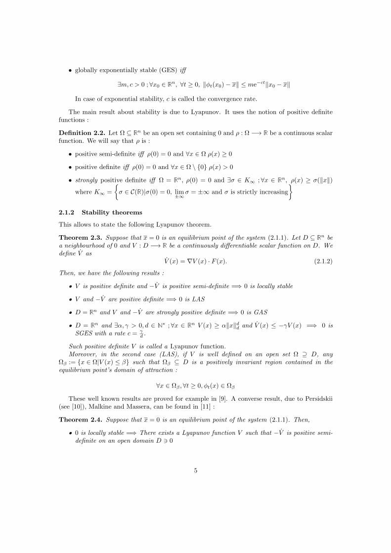
This allows to state the following Lyapunov theorem.

Theorem 2.3. Suppose that x = 0 is an equilibrium point of the system (2.1.1). Let D ⊆ Rn bea neighbourhood of 0 and V : D −→ R be a continuously differentiable scalar function on D. Wedefine V as

V (x) = ∇V (x) · F (x). (2.1.2)

Then, we have the following results :

• V is positive definite and −V is positive semi-definite =⇒ 0 is locally stable

• V and −V are positive definite =⇒ 0 is LAS

• D = Rn and V and −V are strongly positive definite =⇒ 0 is GAS

• D = Rn and ∃α, γ > 0, d ∈ N∗ ;∀x ∈ Rn V (x) ≥ α‖x‖dd and V (x) ≤ −γV (x) =⇒ 0 isSGES with a rate c = γ

d .

Such positive definite V is called a Lyapunov function.Moreover, in the second case (LAS), if V is well defined on an open set Ω ⊇ D, any

Ωβ := x ∈ Ω|V (x) ≤ β such that Ωβ ⊆ D is a positively invariant region contained in theequilibrium point’s domain of attraction :

∀x ∈ Ωβ ,∀t ≥ 0, φt(x) ∈ Ωβ

These well known results are proved for example in [9]. A converse result, due to Persidskii(see [10]), Malkine and Massera, can be found in [11] :

Theorem 2.4. Suppose that x = 0 is an equilibrium point of the system (2.1.1). Then,

• 0 is locally stable =⇒ There exists a Lyapunov function V such that −V is positive semi-definite on an open domain D 3 0

5

• 0 is LAS =⇒ There exists a Lyapunov function V such that −V is positive definite on anopen domain D 3 0

The more general problem of converse theorems in Lyapunov’s theory is adressed in [12].During my internship, I focused on a system which is known to have a LAS equilibrium point.

The aim was to find an appropriate Lyapunov function with the biggest positively invariant Ωβpossible to approximate its Region Of Attraction (ROA). To achieve this goal, I resorted to theSum-of-Squares theory developed in [9] and adapted to power systems by [3].

2.2 Sums of Squares

This subsection sums up the main results from Z. Wloszek’s PhD. thesis [9], which lead toadressing the Lyapunov problems from the Sums Of Squares (SOS) point of view.

2.2.1 General results

We will first introduce the basic concepts of real algebraic geometry.

Definition 2.5. Let n ∈ N∗.

• A monomial in n variables is a mα :

Rn −→ R

x 7−→ xα = xα11 . . . xαn

n

where α ∈ Nn. The degree of a monomial is degmα := |α| =n∑i=1

αi. We will denote byMn

the set of monomials in n variables and, for d ∈ N∗, Mn,d := mα ∈Mn|degmα ≤ d. Awell-known formula states that

|Mn,d| =(n+ dd

).

• A polynomial in n variables is a linear combination of a finite set mαj1≤j≤k of monomials

in n variables.

The degree of a polynomial p is deg p := maxj

degmαj. We will denote by Rn = SpanMn

the set of polynomials in n variables and, for d ∈ N∗, Rn,d := p ∈ Rn|deg p ≤ d.p ∈ Rn is said to be homogeneous iff ∀j ≤ k, degmαj

= deg p = d. Then, ∀λ ∈ R,∀x ∈ Rn,p(λx) = λdp(x).

We will denote by Pn := p ∈ Rn|∀x ∈ Rn, p(x) ≥ 0, and Pn,d := Pn ∩Rn,d.

• p ∈ Rn is a Sum Of Squares (SOS) iff ∃π1, . . . , πk ∈ Rn ; p =k∑j=1

π2j .

We will denote by Σn the set of SOS polynomials, and Σn,d := Σn ∩Rn,d.

Nota : It is obvious that Σn ⊆ Pn (and that a SOS must have an even degree 2d). However,the converse result is false in general. In fact, Hilbert stated in [13] that when we only considerhomogeneous polynomials, Σn,d = Pn,d only in the following cases :

• n = 1 (polynomials in one variable)

• d = 2 (quadratic polynomials)

• n = 2, d = 4 (plane quartics)

6

[14] extends this result to general polynomials. In the general case, we only have Σn,d Pn,d.However, the 17th Hilbert problem, solved by Emil Artin in 1927, states that every p ∈ Pn,d isa sum of squares of rational functions.

It is proved in [15] that SOS polynomials can be parameterized using positive semi-definitesymmetric matrices ; if we denote by Zn,d the vector of all monomials in n variables of degreeless than or equal to d in which mα precedes mβ iff : “degmα < degmβ or if degmα = degmβ

and the first entry of α − β that is strictly negative is preceded by a strictly positive entry”(quoted from [9]), for example

Z2,2(x) =

1x1

x2

x21

x1x2

x22

,

then we have the following theorem :

Theorem 2.6. Let p ∈ Rn,2d. p ∈ Σn,2d iff there exists a matrix Q 0 (symmetric, positivesemi-definite) such that

p(x) = Zn,d(x)TQZn,d(x) (2.2.1)

Such Q 0 is called a Gram matrix for p.

Corollary 2.7. The number of squares in a SOS polynomial in n variables of degree 2d can be

chosen less than or equal to N =

(n+ dd

), which is the size of the vector Zn,d.

All these results are useful when someone wants to determine whether a polynomial p ∈ Rn,2dis SOS or not. For that purpose, we denote by SN (R) the vector space of symmetric squarematrices of size N , and we define the subspace Q0 := Q ∈ SN (R)|ZTn,dQZn,d = 0 and denoteby (Q1, . . . , QK) a base of Q0. Then, we have the following theorem, stated by P.A. Parrilo in[14], for checking if p is SOS :

Theorem 2.8. Let p ∈ Rn,2d, and Q0 be a symmetric matrix (non necessarily positive semi-definite !) such that p(x) = Zn,d(x)TQ0Zn,d(x). Then, the following statements are equivalent:

• p ∈ Σn,2d

• Qp ∩ S+N (R) 6= ∅

• the following LMI11 is feasible :

Q0 +

K∑i=1

λiQi 0 (2.2.2)

Where Qp := (Q0 +Q0) and S+N (R) := Q ∈ SN (R)|Q 0.

11. An LMI is a Linear Matrix Inequality, which general form is A0 +k∑

i=1yiAi 0 where the unknown are the

yi ∈ R and A0, . . . , Ak are fixed symmetric matrices. An LMI is feasible iff there exists y ∈ Rk solution to theproblem. The main methods for solving LMIs are given in [16].

7

Finally, Parrilo [14] gives a theorem which will prove very useful for the search of polynomiallyapunov functions.

Theorem 2.9. Let p0, . . . , pm ∈ Rn. The existence of a1, . . . , am ∈ R such that

p0 +

m∑i=1

aipi ∈ Σn

is an LMI feasibility problem.

Corollary 2.10. Let p0, . . . , pm ∈ Rn. The existence of q1, . . . , qm ∈ Rn such that

p0 +

m∑i=1

qipi ∈ Σn

is an LMI feasibility problem.

Proof. Writing qi =∑j

ai,jmαjallows us to rewrite the problem as

p0 +

m∑i=1

∑j

ai,jmαjpi ∈ Σn

which is exactly the problem considered in Theorem 2.9 with fixed polynomials mαjpi ∈ Rn and

unknown coefficients ai,j ∈ R.

Definition 2.11. The problem of finding the appropriate qi in Corollary 2.10 is called a SumOf Squares Program (SOSP).

The most general SOSP can be formulated as follows (see e.g. [17]) :given (ai,j)0≤i≤K,1≤j≤J ∈ RK×Jn , K ∈ 0, . . . ,K, J ∈ 1 . . . , J, find

p1, . . . , pK ∈ RnpK+1, . . . , pK ∈ Σn

such that

a0,j +

K∑i=1

pi · ai,j = 0 for 1 ≤ j ≤ J , (2.2.3a)

a0,j +

K∑i=1

pi · ai,j ∈ Σn for J + 1 ≤ j ≤ J, (2.2.3b)

Which is equivalent to

a0,j +

K∑i=1

pi · ai,j ∈ Σn for 1 ≤ j ≤ J ,

−a0,j −K∑i=1

pi · ai,j ∈ Σn for 1 ≤ j ≤ J ,

a0,j +

K∑i=1

pi · ai,j ∈ Σn for J + 1 ≤ j ≤ J.

8

In other words, one can always remove equality constraint (2.2.3a).

Thanks to Theorem 2.6, we know that if we fix a maximal degree d for the ai,j and the pi,such a problem is equivalent to finding

Q1, . . . , QK ∈ SN (R)

QK+1, . . . , QK 0

such that

A0,j +

K∑i=1

Qi ·Ai,j = 0 for 1 ≤ j ≤ J , (2.2.4a)

A0,j +

K∑i=1

Qi ·Ai,j 0 for J + 1 ≤ j ≤ J, (2.2.4b)

where the Ai,j ∈ SN (R) are such that ai,j(x) = Zn,d(x)TAi,jZn,d(x), which is an LMI.

Currently, such polynomial optimization problems are solved using the SOSTOOLS packagefor Matlab (see e.g. [18] and [17]). This framework deduces the LMIs from the polynomialproblem and calls SeDuMi’s (or another one) semidefinite programming solver (see e.g. [19])to solve them. Then, it deduces from the LMI solution the solution of the initial polynomialproblem.

2.2.2 The Positivstellensatz

The Positivstellensatz (or P-satz) is a fundamental real algebraic geometry result which allowsto reformulate some complicated problems into simpler ones. It resorts to some algebraic notionswhich we will introduce here.

Definition 2.12. Let g1, . . . , gβ , f1, . . . , fα, h1, . . . , hγ ∈ Rn.

• The Multiplicative Monoid generated by g1, . . . , gβ is defined as

M(g1, . . . , gβ) :=

β∏j=1

gkjj |k1, . . . , kβ ∈ N

(2.2.5)

with the convention M(∅) = 1.

• The Cone generated by f1, . . . , fα is defined as

P(f1, . . . , fα) :=

s0 +

P∑i=1

sibi|P ∈ N, s0, . . . , sP ∈ Σn, b1, . . . , bP ∈M(f1, . . . , fα)

(2.2.6)

with the convention P(∅) = Σn.

• The Ideal generated by h1, . . . , hγ is defined as

I(h1, . . . , hγ) :=

γ∑i=1

hkpk|p1, . . . , pγ ∈ Rn

(2.2.7)

with the convention I(∅) = 0.

9

These notion allow us to introduce the Positivstellensatz, which was demonstrated by M.-FRoy, J. Bochnak and M. Coste in [20] :

Theorem 2.13. Let g1, . . . , gβ , f1, . . . , fα, h1, . . . , hγ ∈ Rn. Then, the following statements areequivalent :

• The set f1(x) ≥ 0, . . . , fα(x) ≥ 0x ∈ Rn g1(x) 6= 0, . . . , gβ(x) 6= 0

h1(x) = 0, . . . , hγ(x) = 0

is empty.

• ∃f ∈ P(f1, . . . , fα), g ∈M(g1, . . . , gβ), h ∈ I(h1, . . . , hγ) ;

f + g2 + h = 0. (2.2.8)

Such f, g, h are called P-satz certificates, or P-satz refutations.

One can find some interesting results around the P-satz and polynomial optimization in [9],but it is not the interest here. Now, we will focus on the research of a polynomial Lyapunovfunction for a polynomial differential system, using the Positivstellensatz.

2.2.3 Application to Lyapunov stability analysis

Let us consider the system (2.1.1), where F is now a polynomial in n variables : F ∈ Rn,and F (0) = 0. We are looking for a domain D ⊂ Rn containing 0 and a Lyapunov functionV : D −→ R.

The first step is to describe D as follows :

D = x ∈ Rn|p(x) ≤ β (2.2.9)

with β > 0 and p ∈ Σn strongly positive definite. This way we obtain a D which is connectedand contains 0. We will focus on the research of a Lyapunov function V ∈ Rn such that −V ispositive definite, in the case of the study of a LAS equilibrium point. The other cases can beadressed in a similar manner.

Such a V must satisfy :

x ∈ Rn|p(x) ≤ β \ 0 ⊂ x ∈ Rn|V (x) > 0 (2.2.10a)

x ∈ Rn|p(x) ≤ β \ 0 ⊂ x ∈ Rn|V (x) < 0 (2.2.10b)

And D must be the largest possible : we first fix p and maximize β. This problem can beformulated in a way which is compatible with the P-satz formalism :

maxV ∈Rn,V (0)=0

β s.t.

x ∈ Rn|p(x) ≤ β, `1(x) 6= 0, V (x) ≤ 0 = ∅

x ∈ Rn|p(x) ≤ β, `2(x) 6= 0, V (x) ≥ 0 = ∅

with `1, `2 ∈ Σn positive definite so as to avoid x = 0. According to the P-satz, this isequivalent to

10

maxV ∈ Rn, V (0) = 0,

s1, . . . , s8 ∈ Σn,

k1, k2 ∈ N∗

β s.t.

s1 + (β − p)s2 − V s3 − V (β − p)s4 + `2k11 = 0

s5 + (β − p)s6 + V s7 + V (β − p)s8 + `2k22 = 0

Then, Σn being a multiplicative group, it is obvious that s ∈ Σn =⇒ `2ki−1i s ∈ Σn, so the

problem can be reduced to

maxV ∈ Rn, V (0) = 0,

s2, s3, s4,∈ Σn,

s6, s7, s8 ∈ Σn

β s.t.

−(β − p)s2 + V s3 + V (β − p)s4 − `1 = s1 ∈ Σn (2.2.13a)

−(β − p)s6 − V s7 − V (β − p)s8 − `2 = s5 ∈ Σn (2.2.13b)

which is, according to Corollary 2.10, an LMI feasibility problem.

The next step is to approximate the ROA of the equilibrium point using a positively invariantΩc = x ∈ Rn|V (x) ≤ c ⊂ D. This can also be formulated as an LMI feasibility problem : weare now studying the problem

max c s.t.

x ∈ Rn|V (x) ≤ c ⊂ x ∈ Rn|p(x) ≤ β. (2.2.14)

i.e.

max c s.t.

x ∈ Rn|V (x) ≤ c, p(x) > β = ∅

i.e.

max c s.t.

x ∈ Rn|c− V (x) ≥ 0, p(x)− β ≥ 0, p(x)− β 6= 0 = ∅

which can be rewritten according to Theorem 2.13 as :

maxs10,s11,s12∈Σn

c s.t.

11

− (c− V )s10 − (p− β)s11 − (c− V )(p− β)s12 − (p− β)2 = s9 ∈ Σn (2.2.15)

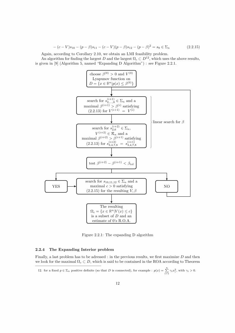
Again, according to Corollary 2.10, we obtain an LMI feasibility problem.An algorithm for finding the largest D and the largest Ωc ⊂ D12, which uses the above results,

is given in [9] (Algorithm 5, named “Expanding D Algorithm”) : see Figure 2.2.1.

choose β(0) > 0 and V (0)

Lyapunov function onD = x ∈ Rn|p(x) ≤ β(0)

search for s(i+1)2,...,8 ∈ Σn and a

maximal β(i+1) > β(i) satisfying(2.2.13) for V (i+1) = V (i)

search for s(i+2)2,6 ∈ Σn,

V (i+2) ∈ Rn and amaximal β(i+2) > β(i+1) satisfying

(2.2.13) for s(i+2)3,4,7,8 = s

(i+1)3,4,7,8

test β(i+2) − β(i+1) < βtol

search for s10,11,12 ∈ Σn and amaximal c > 0 satisfying

(2.2.15) for the resulting V, βYES NO

The resultingΩc = x ∈ Rn|V (x) ≤ cis a subset of D and anestimate of 0’s R.O.A.

linear search for β

Figure 2.2.1: The expanding D algorithm

2.2.4 The Expanding Interior problem

Finally, a last problem has to be adressed : in the previous results, we first maximize D and thenwe look for the maximal Ωc ⊂ D, which is said to be contained in the ROA according to Theorem

12. for a fixed p ∈ Σn positive definite (so that D is connected), for example : p(x) =n∑

i=1γix

2i , with γi > 0.

12

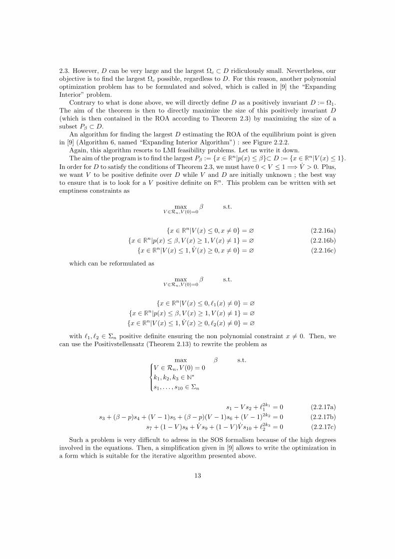
2.3. However, D can be very large and the largest Ωc ⊂ D ridiculously small. Nevertheless, ourobjective is to find the largest Ωc possible, regardless to D. For this reason, another polynomialoptimization problem has to be formulated and solved, which is called in [9] the “ExpandingInterior” problem.

Contrary to what is done above, we will directly define D as a positively invariant D := Ω1.The aim of the theorem is then to directly maximize the size of this positively invariant D(which is then contained in the ROA according to Theorem 2.3) by maximizing the size of asubset Pβ ⊂ D.

An algorithm for finding the largest D estimating the ROA of the equilibrium point is givenin [9] (Algorithm 6, named “Expanding Interior Algorithm”) : see Figure 2.2.2.

Again, this algorithm resorts to LMI feasibility problems. Let us write it down.The aim of the program is to find the largest Pβ := x ∈ Rn|p(x) ≤ β⊂ D := x ∈ Rn|V (x) ≤ 1.

In order for D to satisfy the conditions of Theorem 2.3, we must have 0 < V ≤ 1 =⇒ V > 0. Plus,we want V to be positive definite over D while V and D are initially unknown ; the best wayto ensure that is to look for a V positive definite on Rn. This problem can be written with setemptiness constraints as

maxV ∈Rn,V (0)=0

β s.t.

x ∈ Rn|V (x) ≤ 0, x 6= 0 = ∅ (2.2.16a)

x ∈ Rn|p(x) ≤ β, V (x) ≥ 1, V (x) 6= 1 = ∅ (2.2.16b)

x ∈ Rn|V (x) ≤ 1, V (x) ≥ 0, x 6= 0 = ∅ (2.2.16c)

which can be reformulated as

maxV ∈Rn,V (0)=0

β s.t.

x ∈ Rn|V (x) ≤ 0, `1(x) 6= 0 = ∅x ∈ Rn|p(x) ≤ β, V (x) ≥ 1, V (x) 6= 1 = ∅x ∈ Rn|V (x) ≤ 1, V (x) ≥ 0, `2(x) 6= 0 = ∅

with `1, `2 ∈ Σn positive definite ensuring the non polynomial constraint x 6= 0. Then, wecan use the Positivstellensatz (Theorem 2.13) to rewrite the problem as

maxV ∈ Rn, V (0) = 0

k1, k2, k3 ∈ N∗

s1, . . . , s10 ∈ Σn

β s.t.

s1 − V s2 + `2k11 = 0 (2.2.17a)

s3 + (β − p)s4 + (V − 1)s5 + (β − p)(V − 1)s6 + (V − 1)2k2 = 0 (2.2.17b)

s7 + (1− V )s8 + V s9 + (1− V )V s10 + `2k32 = 0 (2.2.17c)

Such a problem is very difficult to adress in the SOS formalism because of the high degreesinvolved in the equations. Then, a simplification given in [9] allows to write the optimization ina form which is suitable for the iterative algorithm presented above.

13

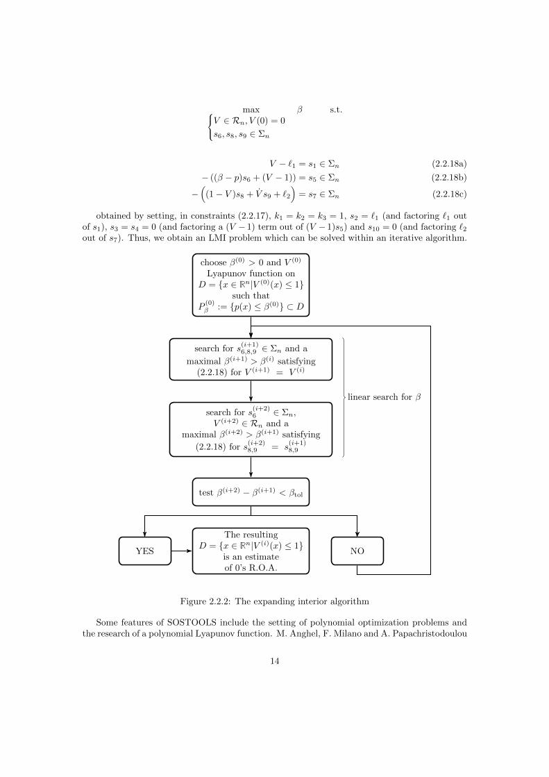
maxV ∈ Rn, V (0) = 0

s6, s8, s9 ∈ Σn

β s.t.

V − `1 = s1 ∈ Σn (2.2.18a)

− ((β − p)s6 + (V − 1)) = s5 ∈ Σn (2.2.18b)

−(

(1− V )s8 + V s9 + `2

)= s7 ∈ Σn (2.2.18c)

obtained by setting, in constraints (2.2.17), k1 = k2 = k3 = 1, s2 = `1 (and factoring `1 outof s1), s3 = s4 = 0 (and factoring a (V − 1) term out of (V − 1)s5) and s10 = 0 (and factoring `2out of s7). Thus, we obtain an LMI problem which can be solved within an iterative algorithm.

choose β(0) > 0 and V (0)

Lyapunov function onD = x ∈ Rn|V (0)(x) ≤ 1

such thatP

(0)β := p(x) ≤ β(0) ⊂ D

search for s(i+1)6,8,9 ∈ Σn and a

maximal β(i+1) > β(i) satisfying(2.2.18) for V (i+1) = V (i)

search for s(i+2)6 ∈ Σn,

V (i+2) ∈ Rn and amaximal β(i+2) > β(i+1) satisfying

(2.2.18) for s(i+2)8,9 = s

(i+1)8,9

test β(i+2) − β(i+1) < βtol

The resultingD = x ∈ Rn|V (i)(x) ≤ 1

is an estimateof 0’s R.O.A.

YES NO

linear search for β

Figure 2.2.2: The expanding interior algorithm

Some features of SOSTOOLS include the setting of polynomial optimization problems andthe research of a polynomial Lyapunov function. M. Anghel, F. Milano and A. Papachristodoulou

14

used this package to implement the expanding interior algorithm in Matlab, which is describedin [3].

3 The Model

3.1 Nominal Operating Equations

3.1.1 Writing the equations

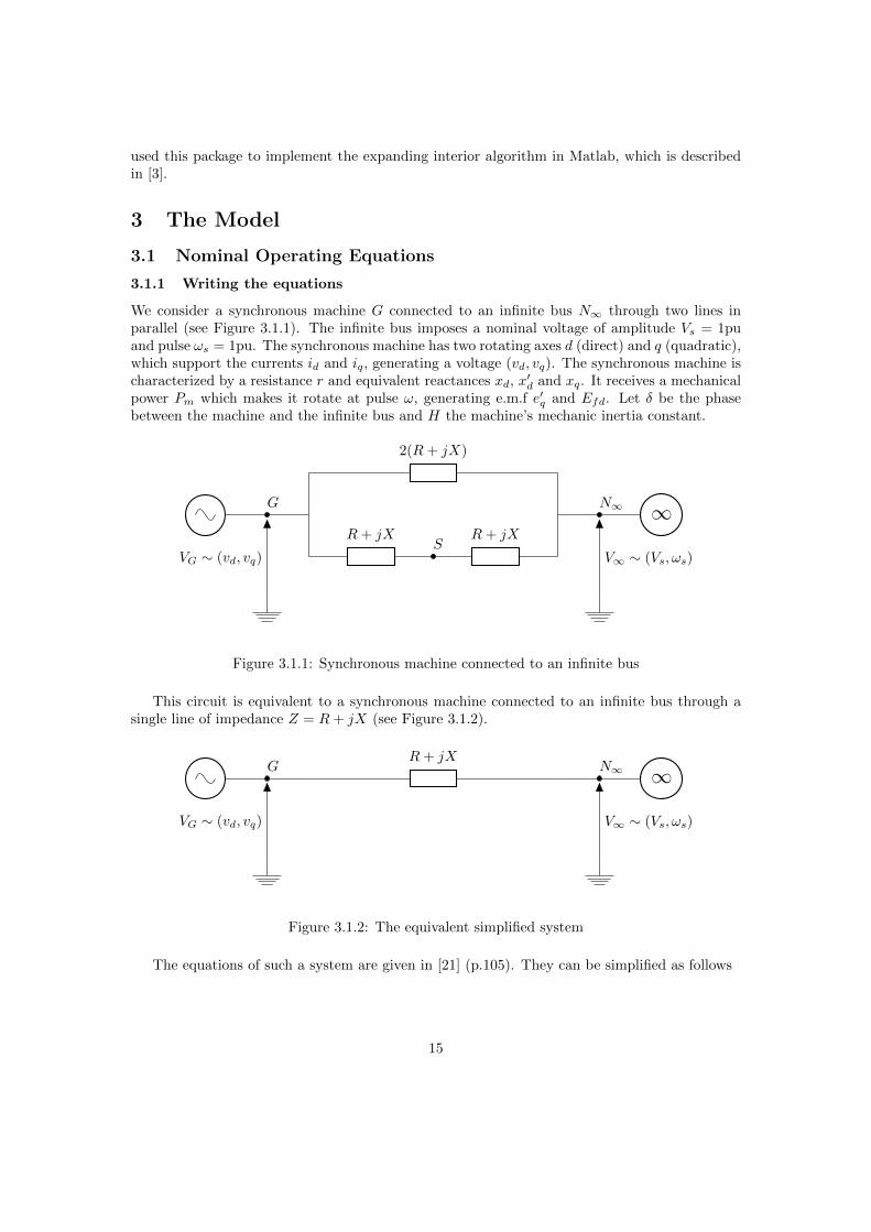
We consider a synchronous machine G connected to an infinite bus N∞ through two lines inparallel (see Figure 3.1.1). The infinite bus imposes a nominal voltage of amplitude Vs = 1puand pulse ωs = 1pu. The synchronous machine has two rotating axes d (direct) and q (quadratic),which support the currents id and iq, generating a voltage (vd, vq). The synchronous machine ischaracterized by a resistance r and equivalent reactances xd, x

′d and xq. It receives a mechanical

power Pm which makes it rotate at pulse ω, generating e.m.f e′q and Efd. Let δ be the phasebetween the machine and the infinite bus and H the machine’s mechanic inertia constant.

G

SR+ jX R+ jX

2(R+ jX)

N∞

VG ∼ (vd, vq) V∞ ∼ (Vs, ωs)

∞

Figure 3.1.1: Synchronous machine connected to an infinite bus

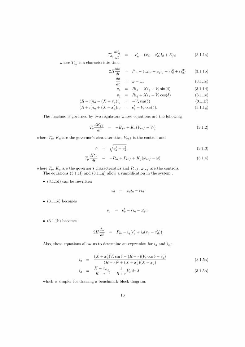
This circuit is equivalent to a synchronous machine connected to an infinite bus through asingle line of impedance Z = R+ jX (see Figure 3.1.2).

GR+ jX

N∞

VG ∼ (vd, vq) V∞ ∼ (Vs, ωs)

∞

Figure 3.1.2: The equivalent simplified system

The equations of such a system are given in [21] (p.105). They can be simplified as follows

15

T ′d0de′qdt

= −e′q − (xd − x′d)id + Efd (3.1.1a)

where T ′d0 is a characteristic time.

2Hdω

dt= Pm − (vdid + vqiq + ri2d + ri2q) (3.1.1b)

dδ

dt= ω − ωs (3.1.1c)

vd = Rid −Xiq + Vs sin(δ) (3.1.1d)

vq = Riq +Xid + Vs cos(δ) (3.1.1e)

(R+ r)id − (X + xq)iq = −Vs sin(δ) (3.1.1f)

(R+ r)iq + (X + x′d)id = e′q − Vs cos(δ). (3.1.1g)

The machine is governed by two regulators whose equations are the following

TadEfddt

= −Efd +Ka(Vref − Vt) (3.1.2)

where Ta, Ka are the governor’s characteristics, Vref is the control, and

Vt =√v2d + v2

q . (3.1.3)

TgdPmdt

= −Pm + Pref +Kg(ωref − ω) (3.1.4)

where Tg, Kg are the governor’s characteristics and Pref , ωref are the controls.The equations (3.1.1f) and (3.1.1g) allow a simplification in the system :

• (3.1.1d) can be rewritten

vd = xqiq − rid

• (3.1.1e) becomes

vq = e′q − riq − x′did

• (3.1.1b) becomes

2Hdω

dt= Pm − iq(e′q + id(xq − x′d))

Also, these equations allow us to determine an expression for id and iq :

iq =(X + x′d)Vs sin δ − (R+ r)(Vs cos δ − e′q)

(R+ r)2 + (X + x′d)(X + xq)(3.1.5a)

id =X + xqR+ r

iq −1

R+ rVs sin δ (3.1.5b)

which is simpler for drawing a benchmark block diagram.

16

3.1.2 Validation of the nominal system

For the simulations (on Matlab, using Simulink and Simscape) we used the following values forthe parameters :

T ′d0 = 9.67 xd = 2.38 x′d = 0.336 xq = 1.21 H = 3 r = 0.002 ωs = ωref = 1 R = 0.01X = 1.185 Vs = 1 Ta = 0.01 Ka = 70 Vref = 1 Tg = 0.4 Kg = 0.5 Pref = 0.7

We also fixed the initial values of the state variables as follows, so as to reach an equilibriumpoint during nominal operating :

e′q(0) = 1.086

ω(0) = 1.05

δ(0) = 1.879

Efd(0) = 32.477

Pm(0) = 1.45

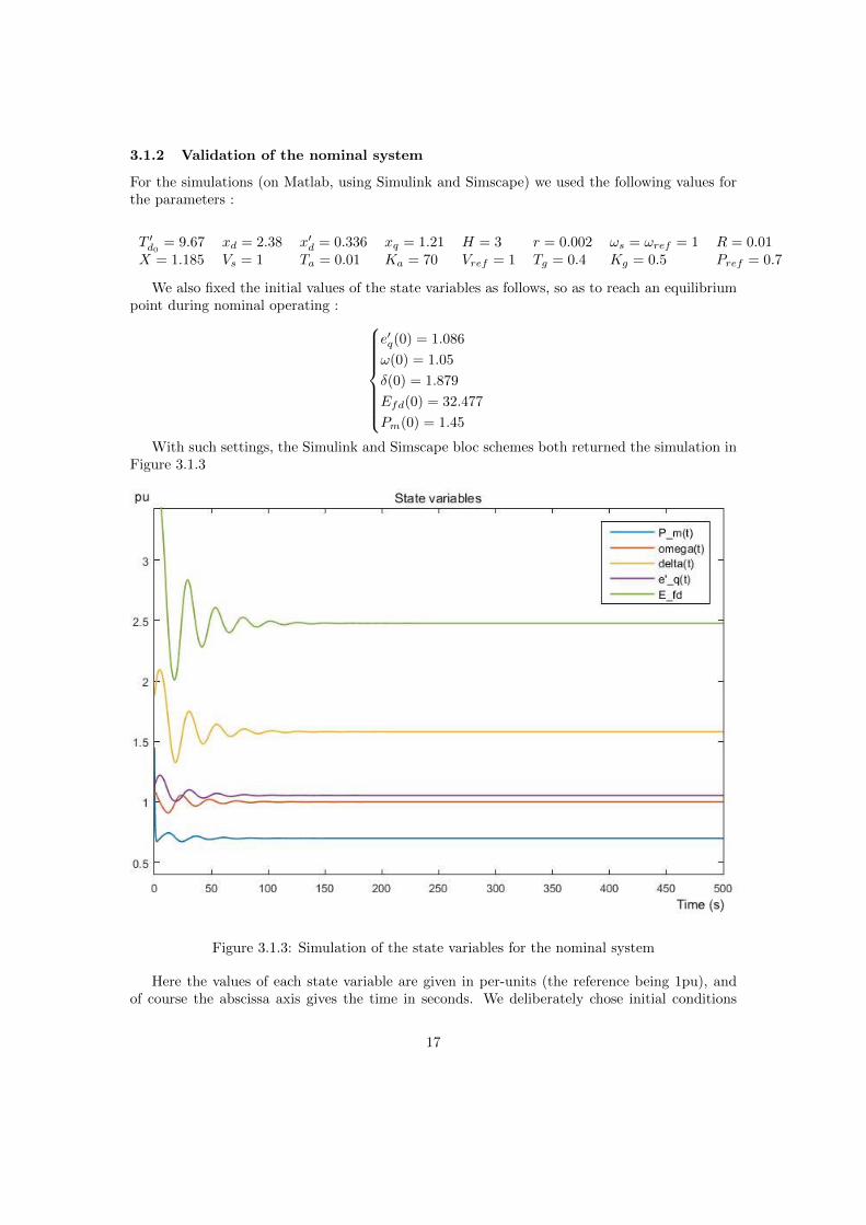
With such settings, the Simulink and Simscape bloc schemes both returned the simulation inFigure 3.1.3

Figure 3.1.3: Simulation of the state variables for the nominal system

Here the values of each state variable are given in per-units (the reference being 1pu), andof course the abscissa axis gives the time in seconds. We deliberately chose initial conditions

17

which were a little far from the equilibrium point so as to clearly observe the damped oscillationsaround it and eventually the stabilization at the main equilibrium point.

At this stage of the study, we can already state that the system has an equilibrium pointaround

δ ' 1.6 ω = ωref = 1 e′q ' 1.1 Efd ' 2.5 Pm = Pref = 0.7.

Then, in order to validate the system, we introduced variations into the controls Vref (1% ofthe nominal value at t = 100s) and Pref (3% of the nominal value at t = 300s), to see how thesystem reacts to small perturbations.

Starting from the previously found equilibrium point, we got the simulation in Figure 3.1.4

Figure 3.1.4: Simulation of the nominal system with perturbations

Here one can see that Efd quickly reacts to an electrical perturbation in Vref , and that amechanical perturbation in Pref leads to slower oscillations of the state variables (especially Efd).

Nota : Despite Efd’s very fast dynamics, one can observe quite slow oscillations in thisvariable. This can be explained by the existence of what is called an interzone mode. Indeed,as it occurs for a mass fixed to a wall through a large spring, here the machine linked to aninfinite bus through a very long line undergoes oscillations which are independent from it’s owndynamics but are due to the global system’s working modes.

18

3.2 The Short-Circuit Model

3.2.1 Writing the short-circuit equations

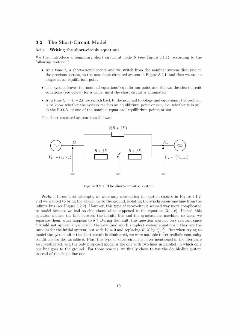
We then introduce a temporary short circuit at node S (see Figure 3.1.1), according to thefollowing protocol :

• At a time tc a short-circuit occurs and we switch from the nominal system discussed inthe previous section, to the new short-circuited system in Figure 3.2.1, and thus we are nolonger at an equilibrium point

• The system leaves the nominal equations’ equilibrium point and follows the short-circuitequations (see below) for a while, until the short circuit is eliminated

• At a time tcl = tc+∆t, we switch back to the nominal topology and equations ; the problemis to know whether the system reaches an equilibrium point or not, i.e. whether it is stillin the R.O.A. of one of the nominal equations’ equilibrium points or not

The short-circuited system is as follows :

G

SR+ jX R+ jX

2(R+ jX)

N∞

VG ∼ (vd, vq) V∞ ∼ (Vs, ωs)

∞

Figure 3.2.1: The short-circuited system

Nota : In our first attempts, we were only considering the system showed in Figure 3.1.2,and we wanted to bring the whole line to the ground, isolating the synchronous machine from theinfinite bus (see Figure 3.2.2). However, this type of short-circuit seemed way more complicatedto model because we had no clue about what happened to the equation (3.1.1c). Indeed, thisequation models the link between the infinite bus and the synchronous machine, so when weseparate them, what happens to δ ? During the fault, this question was not very relevant sinceδ would not appear anywhere in the new (and much simpler) system equations : they are thesame as for the initial system, but with Vs = 0 and replacing R,X by R

2 ,X2 . But when trying to

model the system after the short-circuit is eliminated, we were not able to set realistic continuityconditions for the variable δ. Plus, this type of short-circuit is never mentioned in the literaturewe investigated, and the only proposed model is the one with two lines in parallel, in which onlyone line goes to the ground. For those reasons, we finally chose to use the double-line systeminstead of the single-line one.

19

G SR2 + jX2

R2 + jX2 N∞

VG ∼ (vd, vq) V∞ ∼ (Vs, ωs)

∞ G SR2 + jX2

VG ∼ (vd, vq)

Figure 3.2.2: Our first short-circuit model

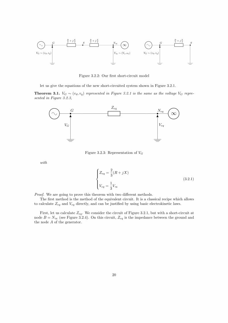
let us give the equations of the new short-circuited system shown in Figure 3.2.1.

Theorem 3.1. VG ∼ (vd, vq) represented in Figure 3.2.1 is the same as the voltage VG repre-sented in Figure 3.2.3,

GZeq

Neq

VG Veq

∞

Figure 3.2.3: Representation of VG

with Zeq =

2

3(R+ jX)

Veq =1

3V∞

(3.2.1)

Proof. We are going to prove this theorem with two different methods.The first method is the method of the equivalent circuit. It is a classical recipe which allows

to calculate Zeq and Veq directly, and can be justified by using basic electrokinetic laws.

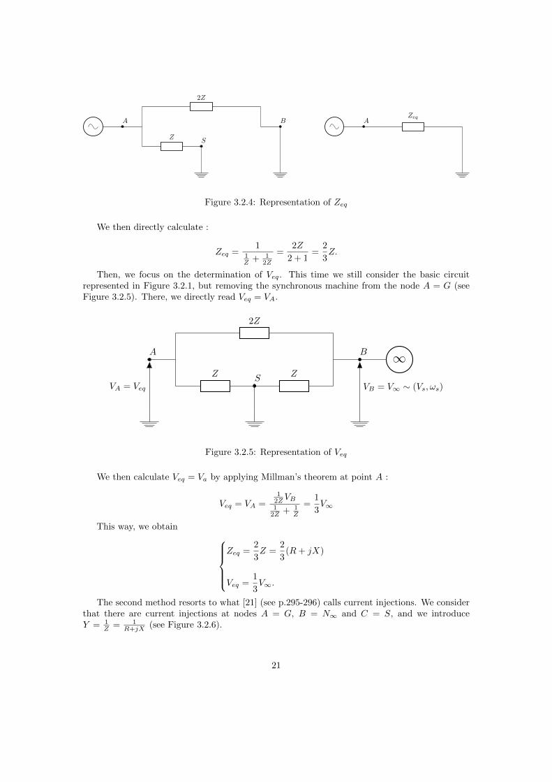
First, let us calculate Zeq. We consider the circuit of Figure 3.2.1, but with a short-circuit atnode B = N∞ (see Figure 3.2.4). On this circuit, Zeq is the impedance between the ground andthe node A of the generator.

20

A

SZ

2Z

B AZeq

Figure 3.2.4: Representation of Zeq

We then directly calculate :

Zeq =1

1Z + 1

2Z

=2Z

2 + 1=

2

3Z.

Then, we focus on the determination of Veq. This time we still consider the basic circuitrepresented in Figure 3.2.1, but removing the synchronous machine from the node A = G (seeFigure 3.2.5). There, we directly read Veq = VA.

A

SZ Z

2Z

B

VA = Veq VB = V∞ ∼ (Vs, ωs)

∞

Figure 3.2.5: Representation of Veq

We then calculate Veq = Va by applying Millman’s theorem at point A :

Veq = VA =1

2ZVB1

2Z + 1Z

=1

3V∞

This way, we obtain Zeq =

2

3Z =

2

3(R+ jX)

Veq =1

3V∞.

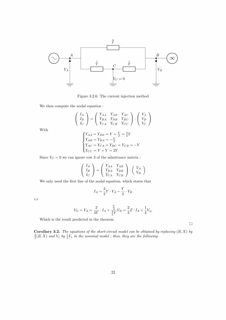
The second method resorts to what [21] (see p.295-296) calls current injections. We considerthat there are current injections at nodes A = G, B = N∞ and C = S, and we introduceY = 1

Z = 1R+jX (see Figure 3.2.6).

21

A

C1Y

1Y

2Y

B

VC = 0

VA VB

∞

Figure 3.2.6: The current injection method

We then compute the nodal equation : IAIBIC

=

YAA YAB YACYBA YBB YBCYCA YCB YCC

· VA

VBVC

With

YAA = YBB = Y + Y2 = 3

2Y

YAB = YBA = −Y2YAC = YCA = YBC = YCB = −YYCC = Y + Y = 2Y.

Since VC = 0 we can ignore row 3 of the admittance matrix : IAIBIC

=

YAA YABYBA YBBYCA YCB

· ( VAVB

)We only need the first line of the nodal equation, which states that

IA =3

2Y · VA −

Y

2· VB

i.e

VG = VA =2

3Y· IA +

Y2

32Y

VB =2

3Z · IA +

1

3V∞

Which is the result predicted in the theorem.

Corollary 3.2. The equations of the short-circuit model can be obtained by replacing (R,X) by23 (R,X) and Vs by 1

3Vs in the nominal model ; thus, they are the following

22

T ′d0de′qdt

= −e′q − (xd − x′d)id + Efd (3.2.2)

2Hdω

dt= Pm − (vdid + vqiq + ri2d + ri2q) (3.2.3)

dδ

dt= ω − ωs (3.2.4)

3vd = 2Rid − 2Xiq + Vs sin(δ) (3.2.5)

3vq = 2Riq + 2Xid + Vs cos(δ) (3.2.6)

(2R+ 3r)id − (2X + 3xq)iq = −Vs sin(δ) (3.2.7)

(2R+ 3r)iq + (2X + 3x′d)id = 3e′q − Vs cos(δ) (3.2.8)

TadEfddt

= −Efd +Ka(Vref − Vt) (3.2.9)

Vt =√v2d + v2

q (3.2.10)

TgdPmdt

= −Pm + Pref +Kg(ωref − ω). (3.2.11)

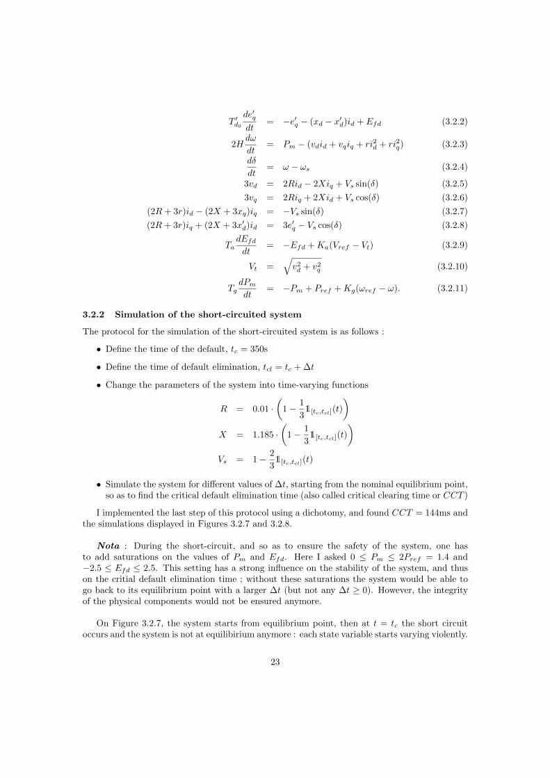
3.2.2 Simulation of the short-circuited system

The protocol for the simulation of the short-circuited system is as follows :

• Define the time of the default, tc = 350s

• Define the time of default elimination, tcl = tc + ∆t

• Change the parameters of the system into time-varying functions

R = 0.01 ·(

1− 1

31[tc,tcl](t)

)X = 1.185 ·

(1− 1

31[tc,tcl](t)

)Vs = 1− 2

31[tc,tcl](t)

• Simulate the system for different values of ∆t, starting from the nominal equilibrium point,so as to find the critical default elimination time (also called critical clearing time or CCT )

I implemented the last step of this protocol using a dichotomy, and found CCT = 144ms andthe simulations displayed in Figures 3.2.7 and 3.2.8.

Nota : During the short-circuit, and so as to ensure the safety of the system, one hasto add saturations on the values of Pm and Efd. Here I asked 0 ≤ Pm ≤ 2Pref = 1.4 and−2.5 ≤ Efd ≤ 2.5. This setting has a strong influence on the stability of the system, and thuson the critial default elimination time ; without these saturations the system would be able togo back to its equilibrium point with a larger ∆t (but not any ∆t ≥ 0). However, the integrityof the physical components would not be ensured anymore.

On Figure 3.2.7, the system starts from equilibrium point, then at t = tc the short circuitoccurs and the system is not at equilibirium anymore : each state variable starts varying violently.

23

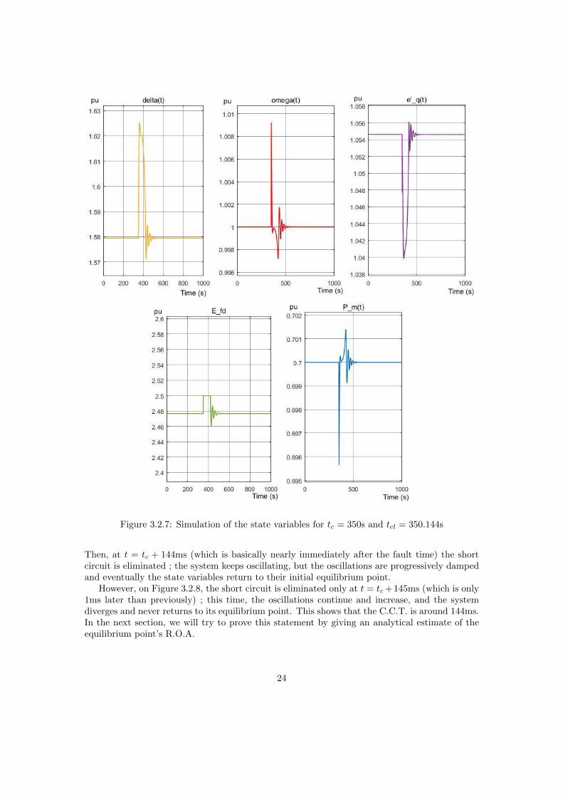
Figure 3.2.7: Simulation of the state variables for tc = 350s and tcl = 350.144s

Then, at t = tc + 144ms (which is basically nearly immediately after the fault time) the shortcircuit is eliminated ; the system keeps oscillating, but the oscillations are progressively dampedand eventually the state variables return to their initial equilibrium point.

However, on Figure 3.2.8, the short circuit is eliminated only at t = tc+145ms (which is only1ms later than previously) ; this time, the oscillations continue and increase, and the systemdiverges and never returns to its equilibrium point. This shows that the C.C.T. is around 144ms.In the next section, we will try to prove this statement by giving an analytical estimate of theequilibrium point’s R.O.A.

24

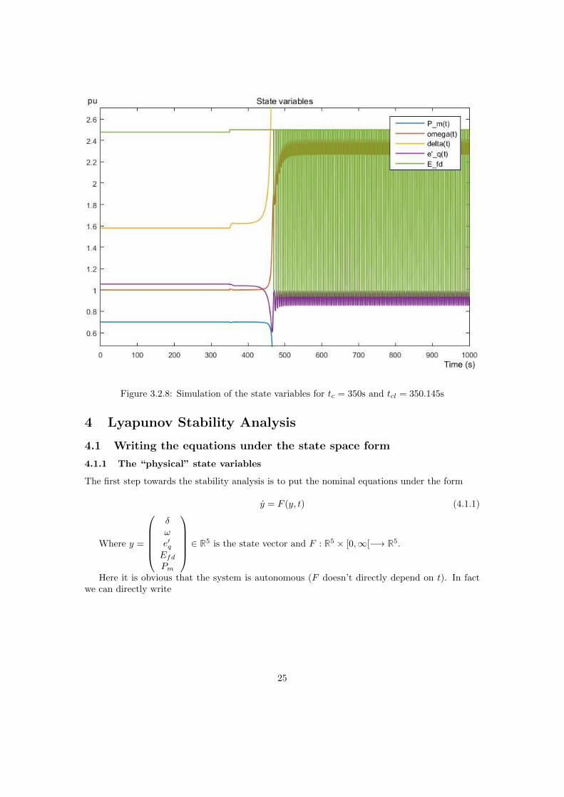
Figure 3.2.8: Simulation of the state variables for tc = 350s and tcl = 350.145s

4 Lyapunov Stability Analysis

4.1 Writing the equations under the state space form

4.1.1 The “physical” state variables

The first step towards the stability analysis is to put the nominal equations under the form

y = F (y, t) (4.1.1)

Where y =

δωe′qEfdPm

∈ R5 is the state vector and F : R5 × [0,∞[−→ R5.

Here it is obvious that the system is autonomous (F doesn’t directly depend on t). In factwe can directly write

25

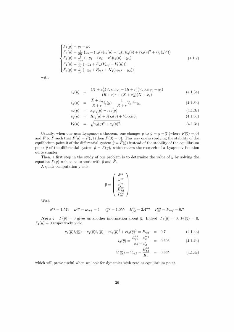
F1(y) = y2 − ωsF2(y) = 1

2H

(y5 − (vd(y)id(y) + vq(y)iq(y) + rid(y)2 + riq(y)2)

)F3(y) = 1

T ′d0

(−y3 − (xd − x′d)id(y) + y4)

F4(y) = 1Ta

(−y4 +Ka(Vref − Vt(y)))

F5(y) = 1Tg

(−y5 + Pref +Kg(ωref − y2))

(4.1.2)

with

iq(y) =(X + x′d)Vs sin y1 − (R+ r)(Vs cos y1 − y3)

(R+ r)2 + (X + x′d)(X + xq)(4.1.3a)

id(y) =X + xqR+ r

iq(y)− 1

R+ rVs sin y1 (4.1.3b)

vd(y) = xqiq(y)− rid(y) (4.1.3c)

vq(y) = Riq(y) +Xid(y) + Vs cos y1 (4.1.3d)

Vt(y) =√vd(y)2 + vq(y)2. (4.1.3e)

Usually, when one uses Lyapunov’s theorem, one changes y to y = y − y (where F (y) = 0)and F to F such that F (y) = F (y) (then F (0) = 0). This way one is studying the stability of theequilibrium point 0 of the differential system ˙y = F (y) instead of the stability of the equilibriumpoinr y of the differential system y = F (y), which makes the research of a Lyapunov functionquite simpler.

Then, a first step in the study of our problem is to determine the value of y by solving theequation F (y) = 0, so as to work with y and F .

A quick computation yields

y =

δeq

ωeq

e′eqqEeqfdP eqm

With

δeq = 1.579 ωeq = ωref = 1 e′eqq = 1.055 Eeqfd = 2.477 P eqm = Pref = 0.7

Nota : F (y) = 0 gives us another information about y. Indeed, F2(y) = 0, F3(y) = 0,F4(y) = 0 respectively yield

vd(y)id(y) + vq(y)iq(y) + rid(y)2 + riq(y)2 = Pref = 0.7 (4.1.4a)

id(y) =Eeqfd − e′eqqxd − x′d

= 0.696 (4.1.4b)

Vt(y) = Vref −EeqfdKa

= 0.965 (4.1.4c)

which will prove useful when we look for dynamics with zero as equilibrium point.

26

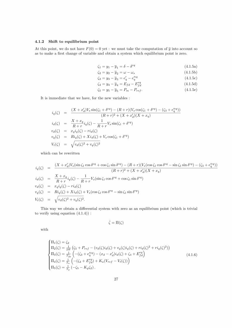
4.1.2 Shift to equilibrium point

At this point, we do not have F (0) = 0 yet : we must take the computation of y into account soas to make a first change of variable and obtain a system which equilibrium point is zero.

ζ1 = y1 − y1 = δ − δeq (4.1.5a)

ζ2 = y2 − y2 = ω − ωs (4.1.5b)

ζ3 = y3 − y3 = e′q − e′eqq (4.1.5c)

ζ4 = y4 − y4 = Efd − Eeqfd (4.1.5d)

ζ5 = y5 − y5 = Pm − Pref . (4.1.5e)

It is immediate that we have, for the new variables :

iq(ζ) =(X + x′d)Vs sin(ζ1 + δeq)− (R+ r)(Vs cos(ζ1 + δeq)− (ζ3 + e′eqq ))

(R+ r)2 + (X + x′d)(X + xq)

id(ζ) =X + xqR+ r

iq(ζ)− 1

R+ rVs sin(ζ1 + δeq)

vd(ζ) = xqiq(ζ)− rid(ζ)

vq(ζ) = Riq(ζ) +Xid(ζ) + Vs cos(ζ1 + δeq)

Vt(ζ) =√vd(ζ)2 + vq(ζ)2

which can be rewritten

iq(ζ) =(X + x′d)Vs(sin ζ1 cos δeq + cos ζ1 sin δeq)− (R+ r)(Vs(cos ζ1 cos δeq − sin ζ1 sin δeq)− (ζ3 + e′eqq ))

(R+ r)2 + (X + x′d)(X + xq)

id(ζ) =X + xqR+ r

iq(ζ)− 1

R+ rVs(sin ζ1 cos δeq + cos ζ1 sin δeq)

vd(ζ) = xqiq(ζ)− rid(ζ)

vq(ζ) = Riq(ζ) +Xid(ζ) + Vs(cos ζ1 cos δeq − sin ζ1 sin δeq)

Vt(ζ) =√vd(ζ)2 + vq(ζ)2.

This way we obtain a differential system with zero as an equilibrium point (which is trivialto verify using equation (4.1.4)) :

ζ = Π(ζ)

with

Π1(ζ) = ζ2

Π2(ζ) = 12H

(ζ5 + Pref − (vd(ζ)id(ζ) + vq(ζ)iq(ζ) + rid(ζ)2 + riq(ζ)2)

)Π3(ζ) = 1

T ′d0

(−(ζ3 + e′eqq )− (xd − x′d)id(ζ) + ζ4 + Eeqfd

)Π4(ζ) = 1

Ta

(−(ζ4 + Eeqfd) +Ka(Vref − Vt(ζ))

)Π5(ζ) = 1

Tg(−ζ5 −Kgζ2) .

(4.1.6)

27

Then, we can proceed to the second step of recasting the system into a polynomial one. Forthis purpose, we will now define V eq := Vt(ζ = 0) = 0.965 (the numerical value was given inequation (4.1.4c)).

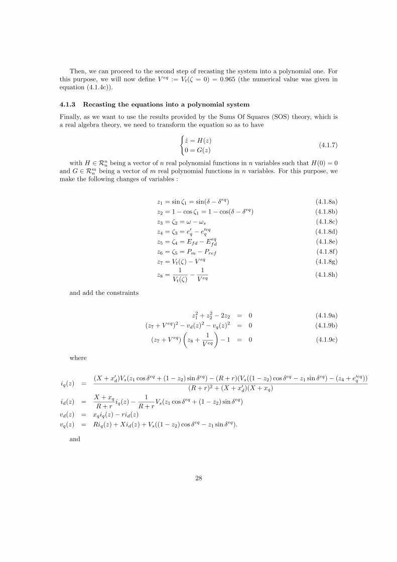
4.1.3 Recasting the equations into a polynomial system

Finally, as we want to use the results provided by the Sums Of Squares (SOS) theory, which isa real algebra theory, we need to transform the equation so as to have

z = H(z)

0 = G(z)(4.1.7)

with H ∈ Rnn being a vector of n real polynomial functions in n variables such that H(0) = 0and G ∈ Rmn being a vector of m real polynomial functions in n variables. For this purpose, wemake the following changes of variables :

z1 = sin ζ1 = sin(δ − δeq) (4.1.8a)

z2 = 1− cos ζ1 = 1− cos(δ − δeq) (4.1.8b)

z3 = ζ2 = ω − ωs (4.1.8c)

z4 = ζ3 = e′q − e′eqq (4.1.8d)

z5 = ζ4 = Efd − Eeqfd (4.1.8e)

z6 = ζ5 = Pm − Pref (4.1.8f)

z7 = Vt(ζ)− V eq (4.1.8g)

z8 =1

Vt(ζ)− 1

V eq(4.1.8h)

and add the constraints

z21 + z2

2 − 2z2 = 0 (4.1.9a)

(z7 + V eq)2 − vd(z)2 − vq(z)2 = 0 (4.1.9b)

(z7 + V eq)

(z8 +

1

V eq

)− 1 = 0 (4.1.9c)

where

iq(z) =(X + x′d)Vs(z1 cos δeq + (1− z2) sin δeq)− (R+ r)(Vs((1− z2) cos δeq − z1 sin δeq)− (z4 + e′eqq ))

(R+ r)2 + (X + x′d)(X + xq)

id(z) =X + xqR+ r

iq(z)−1

R+ rVs(z1 cos δeq + (1− z2) sin δeq)

vd(z) = xqiq(z)− rid(z)vq(z) = Riq(z) +Xid(z) + Vs((1− z2) cos δeq − z1 sin δeq).

and

28

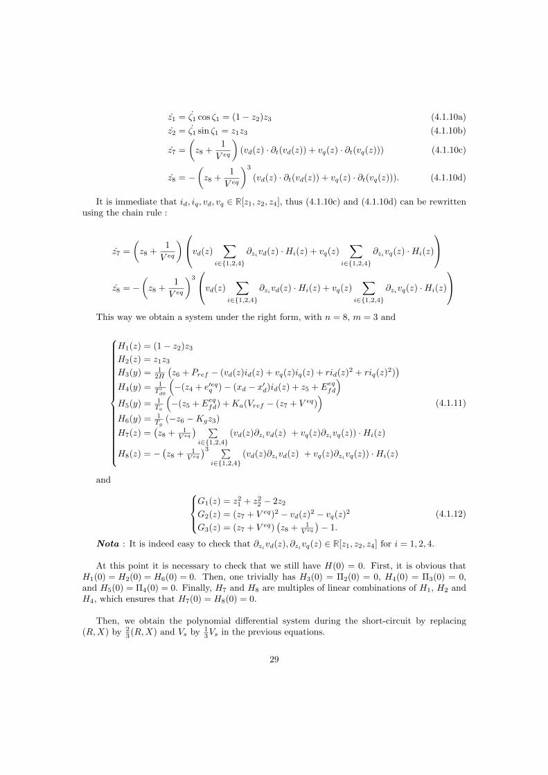
z1 = ζ1 cos ζ1 = (1− z2)z3 (4.1.10a)

z2 = ζ1 sin ζ1 = z1z3 (4.1.10b)

z7 =

(z8 +

1

V eq

)(vd(z) · ∂t(vd(z)) + vq(z) · ∂t(vq(z))) (4.1.10c)

z8 = −(z8 +

1

V eq

)3

(vd(z) · ∂t(vd(z)) + vq(z) · ∂t(vq(z))). (4.1.10d)

It is immediate that id, iq, vd, vq ∈ R[z1, z2, z4], thus (4.1.10c) and (4.1.10d) can be rewrittenusing the chain rule :

z7 =

(z8 +

1

V eq

)vd(z) ∑i∈1,2,4

∂zivd(z) ·Hi(z) + vq(z)∑

i∈1,2,4

∂zivq(z) ·Hi(z)

z8 = −

(z8 +

1

V eq

)3vd(z) ∑

i∈1,2,4

∂zivd(z) ·Hi(z) + vq(z)∑

i∈1,2,4

∂zivq(z) ·Hi(z)

This way we obtain a system under the right form, with n = 8, m = 3 and

H1(z) = (1− z2)z3

H2(z) = z1z3

H3(y) = 12H

(z6 + Pref − (vd(z)id(z) + vq(z)iq(z) + rid(z)

2 + riq(z)2))

H4(y) = 1T ′d0

(−(z4 + e′eqq )− (xd − x′d)id(z) + z5 + Eeqfd

)H5(y) = 1

Ta

(−(z5 + Eeqfd) +Ka(Vref − (z7 + V eq)

)H6(y) = 1

Tg(−z6 −Kgz3)

H7(z) =(z8 + 1

V eq

) ∑i∈1,2,4

(vd(z)∂zivd(z) + vq(z)∂zivq(z)) ·Hi(z)

H8(z) = −(z8 + 1

V eq

)3 ∑i∈1,2,4

(vd(z)∂zivd(z) + vq(z)∂zivq(z)) ·Hi(z)

(4.1.11)

and G1(z) = z2

1 + z22 − 2z2

G2(z) = (z7 + V eq)2 − vd(z)2 − vq(z)2

G3(z) = (z7 + V eq)(z8 + 1

V eq

)− 1.

(4.1.12)

Nota : It is indeed easy to check that ∂zivd(z), ∂zivq(z) ∈ R[z1, z2, z4] for i = 1, 2, 4.

At this point it is necessary to check that we still have H(0) = 0. First, it is obvious thatH1(0) = H2(0) = H6(0) = 0. Then, one trivially has H3(0) = Π2(0) = 0, H4(0) = Π3(0) = 0,and H5(0) = Π4(0) = 0. Finally, H7 and H8 are multiples of linear combinations of H1, H2 andH4, which ensures that H7(0) = H8(0) = 0.

Then, we obtain the polynomial differential system during the short-circuit by replacing(R,X) by 2

3 (R,X) and Vs by 13Vs in the previous equations.

29

4.1.4 A Lie-Blacklund transformation

It is not obvious that the change of variable operated in section 4.1.3 doesn’t affect the dynamicsystem we are looking at. Indeed, we switch from a nonlinear, non-polynomial ordinary differen-tial system, to a system of polynomial differential algebraic equations, with a different numberof state variables.

Usually, one does not change the number of state variables without changing the studiedsystem, because the dimension of the state space is considered an invariant of a dynamic system.However, M. Fliess’ team demonstrated in [22] that, with a good definition of a dynamic system(which in particular preserves trajectories), one can make certain changes of variables withoutmodifying the system, even if the number of states variables changes. For that purpose, oneneeds to introduce some theoretical notions.

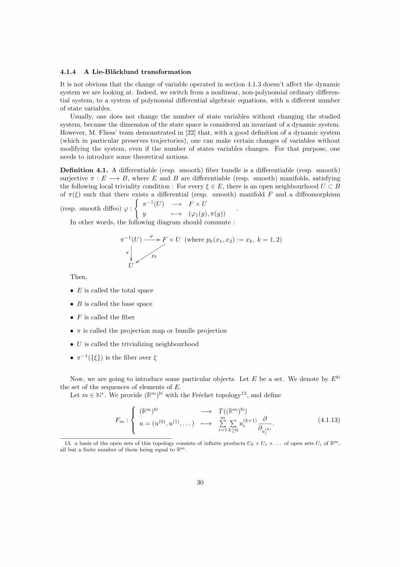
Definition 4.1. A differentiable (resp. smooth) fiber bundle is a differentiable (resp. smooth)surjective π : E −→ B, where E and B are differentiable (resp. smooth) manifolds, satisfyingthe following local triviality condition : For every ξ ∈ E, there is an open neighbourhood U ⊂ Bof π(ξ) such that there exists a differential (resp. smooth) manifold F and a diffeomorphism

(resp. smooth diffeo) ϕ :

π−1(U) −→ F × Uy 7−→ (ϕ1(y), π(y))

.

In other words, the following diagram should commute :

π−1(U)

π

ϕ // F × U

p2yy

U

(where pk(x1, x2) := xk, k = 1, 2)

Then,

• E is called the total space

• B is called the base space

• F is called the fiber

• π is called the projection map or bundle projection

• U is called the trivializing neighbourhood

• π−1(ξ) is the fiber over ξ

Now, we are going to introduce some particular objects. Let E be a set. We denote by EN

the set of the sequences of elements of E.Let m ∈ N∗. We provide (Rm)N with the Frechet topology13, and define

Fm :

(Rm)N −→ T ((Rm)N)

u = (u(0), u(1), . . . ) 7−→m∑i=1

∑k≥0

u(k+1)i

∂

∂u(k)i

.(4.1.13)

13. a basis of the open sets of this topology consists of infinite products U0 × U1 × . . . of open sets Ui of Rm,all but a finite number of them being equal to Rm.

30

A vector field defined on an infinite dimension manifold is said to be differentiable (resp. smooth)iff it is differentiably (resp. smoothly) depending on a finite (but arbitrary) number of coordi-nates.

With such notions, one can define a system as follows.

Definition 4.2. LetM be a smooth manifold, possibly of infinite dimension, and F :M−→ TMa smooth vector field on M.

The pair (M, F ) is a system iff there exists a smooth fiber bundle π :M −→ (Rm)N, for acertain m ∈ N∗, such that every fiber is finite-dimensional with locally constant dimension, andfor all ξ ∈M

∇π(ξ) · F (ξ) = Fm(π(ξ)) (4.1.14)

This allows us to define :

• local coordinates ξ = (x, u) , where u = π(ξ) and x ∈ Rn, in which

F (ξ) = f(x, u)∂

∂x+

m∑i=1

∑k≥0

u(k+1)i

∂

∂u(k)i

(4.1.15)

with f depending on a finite number of coordinates.

• trajectories t 7−→ ξ(t) := (x(t), u(t)) such that ξ(t) = F (ξ(t)) i.e. x(t) = f(x(t), u(t))

This way, one obtains a controlled differential system with finite dimension. However, thedefinition of the state variables and the control variables entirely depends on the choice of π,which makes this definition fit also the non-controlled systems. In fact, the presence of a controldoes not depend on the system, but on the projection π one uses.

Now let us introduce the notion of Lie-Blacklund transformation.

Definition 4.3. Let (M, F ), (N , H) be two systems, Φ :M C∞

−→ N , p ∈M and q := Φ(p) ∈ N .Then,

• if ξ is a trajectory of (M, F ) in a neighbourhood of p, then ζ := Φ ξ stays in a neighbour-hood of q and we have

ζ(t) = ∇Φ(ξ(t)) · F (ξ(t)) (4.1.16)

which holds even in infinite dimension : everything depends only on a finite number ofcoordinates.

• Φ is an endogenous transformation iff, for any ξ in a neighbourhood of p

∇Φ(ξ) · F (ξ) = H(Φ(ξ)) (4.1.17)

(we say that F and H are Φ-related at (p, q) ; then ζ = H(ζ)) and Φ has a smooth inverseΨ (then, H and F are automatically Ψ-related).

• Φ is a Lie-Blacklund isomorphism iff we locally have

TΦ(span(F )) = span(H)

31

and Φ has a smooth inverse Ψ such that TΨ(span(H)) = span(F )14. In other words, for ξin a neighbourhood of p and ζ in a neighbourhood of q, we should have

(∇Φ(ξ))(R · F (ξ)) = R ·H(Φ(ξ)) (4.1.18a)

(∇Ψ(ζ))(R ·H(ζ)) = R · F (Ψ(ζ)) (4.1.18b)

From this definition, it is obvious that an endogenous transformation (which is a particularcase of Lia-Blacklund isomorphism) preserves the trajectories (and so the stability properties) ofa system, which is exactly what we need for our transformations not to modify the ROA of ourLAS equilibrium point.

In fact, in our case, a very particular case of such a transformation is being used, since wework in finite dimension, and we resort to an endogenous transformation. Let us prove this fact.

First, it is obvious that a translation on the state variables is an endogenous transforma-tion, and that the composition of two endogenous transformations is still an endogenous trans-formation. Thus, the shifting (R5, F ) −→ (R5,Π) operated in section 4.1.2 is an endogenoustransformation and what we have to prove is that the transformation

Φ :

R5 −→ M := z ∈ R8|G(z) = 0

(ζ1, . . . , ζ5) 7−→(

sin(ζ1), 1− cos(ζ1), ζ2, ζ3, ζ4, ζ5, Vt(ζ)− V eq, 1

Vt(ζ)− 1

V eq

)is an endogenous transformation between the systems (R5,Π) and (M, H), with the Π, G,

H and Vt functions introduced in the previous sections, i.e. that Φ has a smooth inverse Ψ, andthat H(Φ(ζ)) = ∇Φ(ζ) ·Π(ζ).

First, let us prove that Φ is well defined, i.e. that G Φ = 0. We have

G1(Φ(ζ)) = sin2 ζ1 + (1− cos ζ1)2 − 2(1− cos ζ1)

= sin2 ζ1 + 1− 2 cos ζ1 + cos2 ζ1 − 2 + 2 cos ζ1

= 1 + 1− 2− 2 cos ζ1 + 2 cos ζ1 = 0

G2(Φ(ζ)) = ((Vt(ζ)− V eq) + V eq)2 − vd(ζ)2 − vq(ζ)2

= Vt(ζ)2 − vd(ζ)2 − vq(ζ)2 = 0

G3(Φ(ζ)) = ((Vt(ζ)− V eq) + V eq)

((1

Vt(ζ)− 1

V eq

)+

1

V eq

)− 1

= Vt(ζ)1

Vt(ζ)− 1 = 0

Nota : To prove that Φ is well defined, we also need Vt(ζ) 6= 0. In fact, the physics en-sure that Vt 6= 0 ∀t because short-circuits cannot occur inside the synchronous machine. So wealready know that starting from any physically relevant point, the system won’t reach the sety ∈ R5|Vt(y) = 0, which is sufficient here.

14. A distribution D :=span(V1, . . . , Vk) being intuitively defined on a manifold M byD(x) =span(V1(x), . . . , Vk(x)) ⊂ TM, where V1, . . . , Vk are vector fields on M. TΦ is a notation todenote the application ξ 7−→ ∇Φ(ξ) · •.

32

Then, we want to find a smooth inverse Ψ to Φ. We define :

Ψ(z) = (arg((1− z2) + iz1), z3, z4, z5, z6) (4.1.19)

Now, let us show that Ψ is well defined and a smooth inverse of Φ.First, arg((1 − z2) + iz1) is well defined and smooth iff (1 − z2) + iz1 6= 0. This is always

true since the constraint (4.1.9a) ensures z21 + z2

2 − 2z2 = 0 : if 1− z2 = 0 then it forces z1 = ±1; conversely, z1 = 0 =⇒ 1− z2 = ±1. So Ψ is well defined.

Plus, it is obvious that Ψ is smooth and that Ψ(Φ(ζ)) = (arg(cos ζ1 + i sin ζ1), ζ2, ζ3, ζ4, ζ5) = (ζ1, ζ2, ζ3, ζ4, ζ5).

Finally, H(Φ(ζ)) = ∇Φ(ζ) ·Π(ζ) is obvious because H was precisely defined so as to obtainthis equality (using the chain rule).

Nota : Here the constraints (4.1.9b) and (4.1.9c) do not seem to be relevant since onlyconstraint (4.1.9a) is used to show that Ψ is a well defined smooth inverse of Φ. However, thesetwo constraints are fundamental to define properly the dynamics of the recasted system (see H5,H7 and H8).

Also, we see that z7 + V eq and z8 + 1V eq are allowed to be negative in the recasted sys-

tem, but that Vt is forced to be positive in the original one. This actually is not a problemsince we start from a physically relevant point z7 + V eq > 0 and the dynamics of the system donot allow it to reach the hyperplan z7 +V eq = 0, so we are always working in the good conditions.

Finally, we have proved that the initial physical system and the recasted system we are goingto study are equivalent via an endogenous transformation, which means they have the sametrajectories and stability properties.

4.2 Estimating the R.O.A. using SOSTOOLS

4.2.1 Statement of the problem and structure of the codes

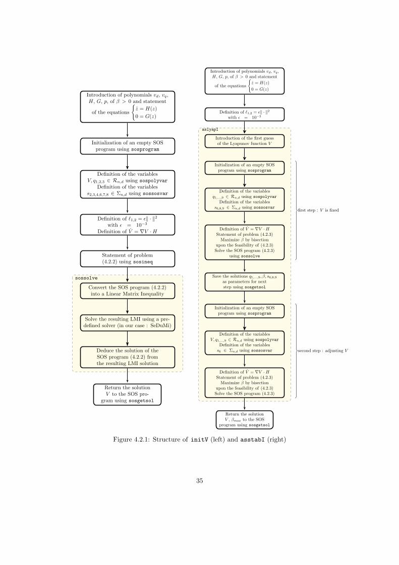
As it was explained in section 2.2.4, the expanding D algorithm has some flaws which make itless efficient than the expanding interior algorithm. For this reason, it was not implemented in[3], and I did not implement it during my internship. Instead, we directly used the expandinginterior algorithm, through three distinct scripts.

The first script, named initV, finds a candidate Lyapunov function to initialize the algorithm.The second one, named asstabI, is the structure of the expanding interior algorithm : it statesthe optimization problem we are aiming to solve, coordinates the optimization of the variablesand returns the result. The third code, which is called by asstabI, is named aslyapI and carriesout the two main optimization steps of the expanding interior algorithm, corresponding to theoptimization loop.

Here, the addition of the equality constraints G(z) = 0 only influences the definition of thedomain D on which we are looking for a Lyapunov function : now we have

D = z ∈ R8|p(z) ≤ β ;G(z) = 0. (4.2.1)

This leads, according to theorem 2.13 (P-satz), to enriched problems :Looking for a Lyapunov function on D is equivalent to

33

−(β − p)s2 + V s3 + V (β − p)s4 − `1 −∑

i=1,2,3

qiGi = s1 ∈ Σn (4.2.2a)

−(β − p)s6 − V s7 − V (β − p)s8 − `2 −∑

i=1,2,3

qiGi = s5 ∈ Σn (4.2.2b)

and the expanding interior problem can be rewritten as

V − `1 −∑

i=1,2,3

qiGi = s1 ∈ Σn (4.2.3a)

− ((β − p)s6 + (V − 1))−∑

i=1,2,3

qi+3Gi = s5 ∈ Σn (4.2.3b)

−(

(1− V )s8 + V s9 + `2

)−∑

i=1,2,3

qi+6Gi = s7 ∈ Σn (4.2.3c)

Where q1,...,9 are free polynomial variables (∑qiGi is therefore the definition of an element

of the ideal I(G1, G2, G3)).

The scripts involved are described in Figure 4.2.1. They were initially written by M.Angheland S.Kundu, and then rearranged by myself so as to fit with my problem, after I entirely readand understood them.

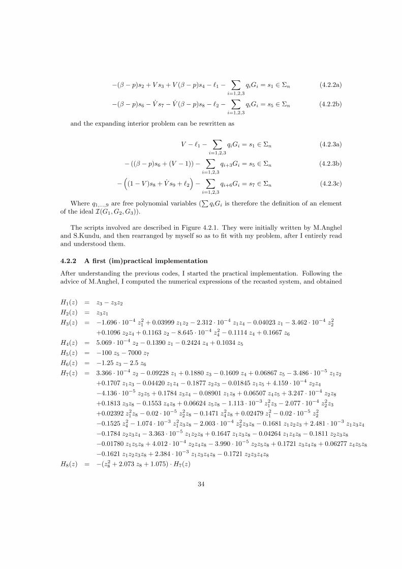
4.2.2 A first (im)practical implementation

After understanding the previous codes, I started the practical implementation. Following theadvice of M.Anghel, I computed the numerical expressions of the recasted system, and obtained

H1(z) = z3 − z3z2

H2(z) = z3z1

H3(z) = −1.696 · 10−4 z21 + 0.03999 z1z2 − 2.312 · 10−4 z1z4 − 0.04023 z1 − 3.462 · 10−4 z2

2

+0.1096 z2z4 + 0.1163 z2 − 8.645 · 10−4 z24 − 0.1114 z4 + 0.1667 z6

H4(z) = 5.069 · 10−4 z2 − 0.1390 z1 − 0.2424 z4 + 0.1034 z5

H5(z) = −100 z5 − 7000 z7

H6(z) = −1.25 z3 − 2.5 z6

H7(z) = 3.366 · 10−4 z2 − 0.09228 z1 + 0.1880 z3 − 0.1609 z4 + 0.06867 z5 − 3.486 · 10−5 z1z2

+0.1707 z1z3 − 0.04420 z1z4 − 0.1877 z2z3 − 0.01845 z1z5 + 4.159 · 10−4 z2z4

−4.136 · 10−5 z2z5 + 0.1784 z3z4 − 0.08901 z1z8 + 0.06507 z4z5 + 3.247 · 10−4 z2z8

+0.1813 z3z8 − 0.1553 z4z8 + 0.06624 z5z8 − 1.113 · 10−3 z21z3 − 2.077 · 10−4 z2

2z3

+0.02392 z21z8 − 0.02 · 10−5 z2

2z8 − 0.1471 z24z8 + 0.02479 z2

1 − 0.02 · 10−5 z22

−0.1525 z24 − 1.074 · 10−3 z2

1z3z8 − 2.003 · 10−4 z22z3z8 − 0.1681 z1z2z3 + 2.481 · 10−3 z1z3z4

−0.1784 z2z3z4 − 3.363 · 10−5 z1z2z8 + 0.1647 z1z3z8 − 0.04264 z1z4z8 − 0.1811 z2z3z8

−0.01780 z1z5z8 + 4.012 · 10−4 z2z4z8 − 3.990 · 10−5 z2z5z8 + 0.1721 z3z4z8 + 0.06277 z4z5z8

−0.1621 z1z2z3z8 + 2.384 · 10−3 z1z3z4z8 − 0.1721 z2z3z4z8

H8(z) = −(z28 + 2.073 z8 + 1.075) ·H7(z)

34

sossolve

Introduction of polynomials vd, vq,H, G, p, of β > 0 and statement

of the equations

z = H(z)

0 = G(z)

Initialization of an empty SOSprogram using sosprogram

Definition of the variablesV, q1,2,3 ∈ Rn,d using sospolyvar

Definition of the variabless2,3,4,6,7,8 ∈ Σn,d using sossosvar

Definition of `1,2 = ε‖ · ‖2with ε = 10−3

Definition of V = ∇V ·H

Statement of problem(4.2.2) using sosineq

Convert the SOS program (4.2.2)into a Linear Matrix Inequality

Solve the resulting LMI using a pre-defined solver (in our case : SeDuMi)

Deduce the solution of theSOS program (4.2.2) fromthe resulting LMI solution

Return the solutionV to the SOS pro-

gram using sosgetsol

aslyapI

Introduction of polynomials vd, vq,H, G, p, of β > 0 and statement

of the equations

z = H(z)

0 = G(z)

Definition of `1,2 = ε‖ · ‖2with ε = 10−3

Introduction of the first guessof the Lyapunov function V

Initialization of an empty SOSprogram using sosprogram

Definition of the variablesq1,...,9 ∈ Rn,d using sospolyvar

Definition of the variabless6,8,9 ∈ Σn,d using sossosvar

Definition of V = ∇V ·HStatement of problem (4.2.3)

Maximize β by bisectionupon the feasibility of (4.2.3)

Solve the SOS program (4.2.3)using sossolve

Save the solutions q1,...,9, β, s6,8,9

as parameters for nextstep using sosgetsol

Initialization of an empty SOSprogram using sosprogram

Definition of the variablesV, q1,...,9 ∈ Rn,d using sospolyvar

Definition of the variabless6 ∈ Σn,d using sossosvar

Definition of V = ∇V ·HStatement of problem (4.2.3)

Maximize β by bisectionupon the feasibility of (4.2.3)

Solve the SOS program (4.2.3)

Return the solutionV , βmax to the SOS

program using sosgetsol

first step : V is fixed

second step : adjusting V

Figure 4.2.1: Structure of initV (left) and asstabI (right)

35

and

G1(z) = z21 + z2

2 − 2 z2

G2(z) = −0.04880 z21 − 9.961 · 10−4 z1z2 + 0.3442 z1z4 + 0.3640 z1 − 0.2552 z2

2 + 1.420 · 10−4 z2z4

+0.5106 z2 − 0.6070 z24 − 1.280 z4 + z2

7 + 1.929 z7

G3(z) = 1.037 z7 + 0.9646 z8 + z7z8

This formulation allows to check that 0 is an admissible working point (G(0) = 0) and anequilibrium point for the recasted system (H(0) = 0).

It is also worth noting that the recasting is even more costly than initially expected : wealready knew that this operation would increase the dimension of the state space by 3 (we switchfrom R5 to R8) and that it would add three equality constraints (G(z) = 0). What was notobvious in the non-numerical formulation, was that the new dynamics vector field H is of degree6, while F , the initial one, is only quadratic.

This leads to a huge computation time : the first algorithm (initV), which is also the simplest,took over two hours to run, and the next one (asstabI) did not terminate (or at least, it wouldhave taken more than several days).

Plus, we were already considering a simplified system in which the saturations are not takeninto account. Adding them to the model would be simple (we just have to add some moreinequality constraints to the definition of D, and consequently some more SOS variables to theproblem) but it would increase the computation time which was already skyrocketting.

As a result, we decided to adress an intermediate problem before solving this one.

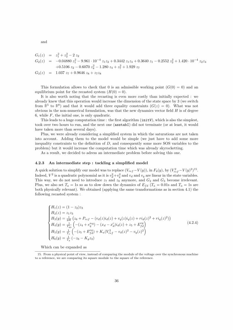
4.2.3 An intermediate step : tackling a simplified model

A quick solution to simplify our model was to replace (Vref−V (y)), in F4(y), by (V 2ref−V (y)2)15.

Indeed, V 2 is a quadratic polynomial as it is v2d+v2

q and vd and vq are linear in the state variables.This way, we do not need to introduce z7 and z8 anymore, and G2 and G3 become irrelevant.Plus, we also set Ta = 1s so as to slow down the dynamics of Efd (Ta = 0.01s and Ta = 1s areboth physically relevant). We obtained (applying the same transformations as in section 4.1) thefollowing recasted system :

H1(z) = (1− z2)z3

H2(z) = z1z3

H3(y) = 12H

(z6 + Pref − (vd(z)id(z) + vq(z)iq(z) + rid(z)

2 + riq(z)2))

H4(y) = 1T ′d0

(−(z4 + e′eqq )− (xd − x′d)id(z) + z5 + Eeqfd

)H5(y) = 1

Ta

(−(z5 + Eeqfd) +Ka(V 2

ref − vd(z)2 − vq(z)2)

H6(y) = 1Tg

(−z6 −Kgz3)

(4.2.4)

Which can be expanded as

15. From a physical point of view, instead of comparing the module of the voltage over the synchronous machineto a reference, we are comparing its square module to the square of the reference.

36

H1(z) = z3 − z3z2

H2(z) = z3z1

H3(z) = −0.001579 z21 + 0.03987 z1z2 − 0.004644 z1z4 − 0.04484 z1 + 0.001464 z2

2 + 0.1095 z2z4

+0.1142 z2 − 0.0008645 z24 − 0.1113 z4 + 0.1667 z6

H4(z) = 0.1034 z5 − 0.005091 z2 − 0.2424 z4 − 0.1389 z1

H5(z) = −3.437 z21 + 1.094 z1z2 + 24.07 z1z4 + 24.67 z1 − 17.85 z2

2 + 0.9804 z2z4 + 36.74 z2 − 42.49 z24

−91.91 z4 − 1.000 z5

H6(z) = −1.25 z3 − 2.5 z6

and

G(z) = z21 + z2

2 − 2z2 (4.2.5)

Nota : Of course, in this case the values of δeq, e′eqq and Eeqfd are different from before sincethe initial F is a little different. Indeed, here a simple computation leads to

δeq = 1.539 ωeq = ωref = 1 e′eqq = 1.070 Eeqfd = 2.459 P eqm = Pref = 0.7

Starting from this point, and without introducing any saturations (so as to keep a simplemodel), we could simulate the short circuit and estimate the C.C.T. : CCT = 4.057 s.

Figure 4.2.2: Simulation of the state variables for the simplified system and tc = 350s andtcl = 354.057s

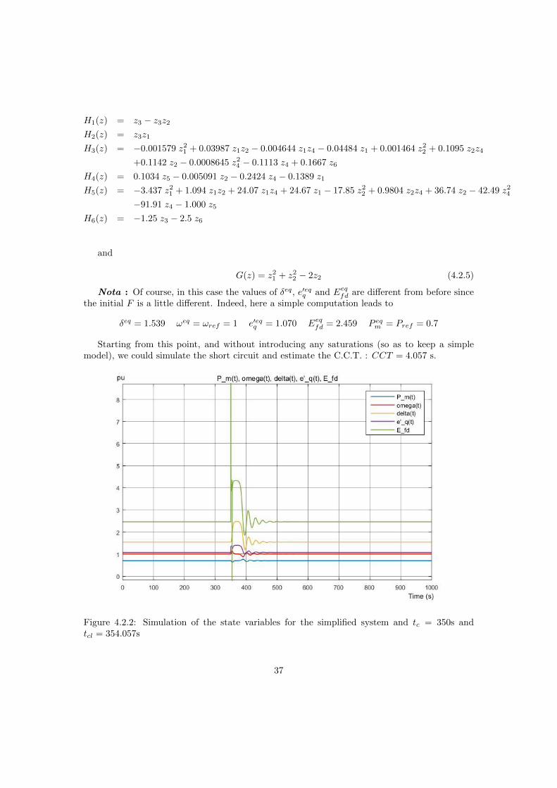
37

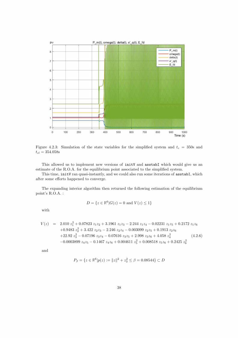
Figure 4.2.3: Simulation of the state variables for the simplified system and tc = 350s andtcl = 354.058s

This allowed us to implement new versions of initV and asstabI which would give us anestimate of the R.O.A. for the equilibrium point associated to the simplified system.

This time, initV ran quasi-instantly, and we could also run some iterations of asstabI, whichafter some efforts happened to converge.

The expanding interior algorithm then returned the following estimation of the equilibriumpoint’s R.O.A. :

D = z ∈ R6|G(z) = 0 and V (z) ≤ 1

with

V (z) = 2.010 z21 + 0.07823 z1z2 + 3.1961 z1z3 − 2.244 z1z4 − 0.02231 z1z5 + 0.2172 z1z6

+0.9483 z22 + 3.422 z2z3 − 2.246 z2z4 − 0.003099 z2z5 + 0.1913 z2z6

+22.92 z23 − 0.07196 z3z4 − 0.07616 z3z5 + 2.998 z3z6 + 4.058 z2

4 (4.2.6)

−0.0003899 z4z5 − 0.1467 z4z6 + 0.004611 z25 + 0.008518 z5z6 + 0.2425 z2

6

and

Pβ = z ∈ R6|p(z) := ‖z‖2 + z23 ≤ β = 0.08544 ⊂ D

38

4.2.4 Intrepretation of the results

In order to conclude the transient stability analysis, the results of the expanding interior algo-rithm had to be interpreted in terms of performance (comparison between what the algorithmyields and the actual R.O.A.) and of C.C.T.

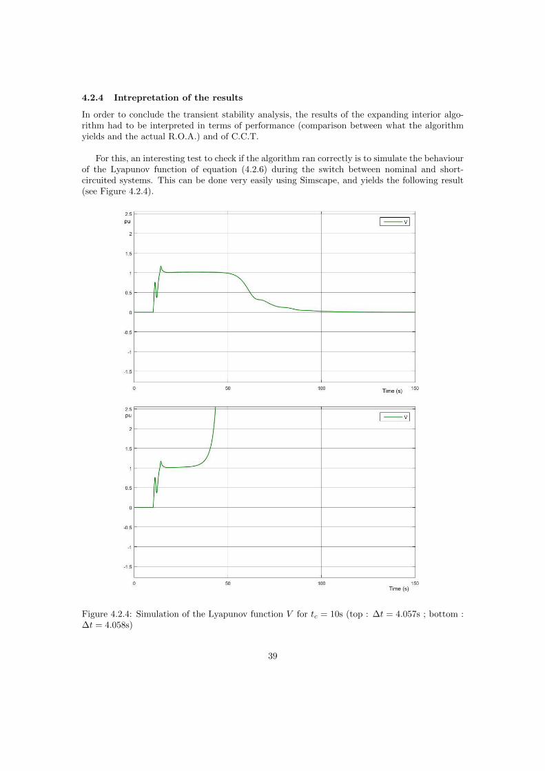
For this, an interesting test to check if the algorithm ran correctly is to simulate the behaviourof the Lyapunov function of equation (4.2.6) during the switch between nominal and short-circuited systems. This can be done very easily using Simscape, and yields the following result(see Figure 4.2.4).

Figure 4.2.4: Simulation of the Lyapunov function V for tc = 10s (top : ∆t = 4.057s ; bottom :∆t = 4.058s)

39

On this figure, one can check that in the stable case (∆t = 4.057s), V converges to 0 meanwhilein the unstable case (∆t = 4.058s), V quickly diverges, which is normal when one is observing aLyapunov function.

However, if the R.O.A. estimation were perfect, in the stable case V should not surpass 1. Infact, V behaves the same way in both cases, until it returns to 1.

This could first seem strange because it means that V has the same behaviour during theshort circuit in both cases. Nevertheless, this is only relevant if the state variables remain in adomain where V is a Lyapunov function. Here V is assured to be Lyapunov only on z|V (z) ≤ 1,so as soon as V surpasses 1, its behaviour is not so relevant (however, it is still relevant to see Vconverge to 0 : here we have V (z) ≤ 1 so its behaviour makes sense).

In fact, the simulation of V only allowed us to check that V behaves like a Lyapunov functionwhen it is below 1 (i.e. that V converges to 0 in the stable case).

Nevertheless, this simulation also allows us to give an estimate of the C.C.T. using ourestimate of the R.O.A. : indeed, tcl is the time at which V surpasses 1. As a result, we get an

estimate CCT of CCT :

CCT = 3.591 s (4.2.7)

Which is not so far from the actual CCT = 4.057 s...

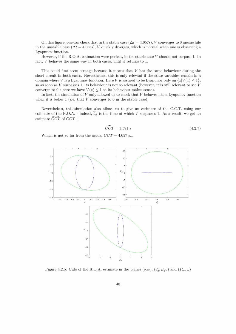
Figure 4.2.5: Cuts of the R.O.A. estimate in the planes (δ, ω), (e′q, Efd) and (Pm, ω)

40

In order to go further in the study of the R.O.A., I represented some cuts of D and Pβ in2D spaces : among the 5 shifted (so that the equilibrium point is zero) state variables I selectedthe two I wanted to see, called them x and y and forced the three others to zero. Then I traced2D plots of the level sets z|V (z) = 1 = ∂D (in green) and z|p(z) = β = ∂Pβ (in blue). Irepeated this process for (x, y) = (δ, ω), (e′q, Efd) and (Pm, ω) and obtained Figure 4.2.5

A way to roughly (but easily) compare this estimate to the actual R.O.A. consists in simu-lating the nominal system with initial conditions at equilibrium except for one state variable y,and to progressively increase its initial value yinit until the system does not reach its equilibriumpoint anymore.

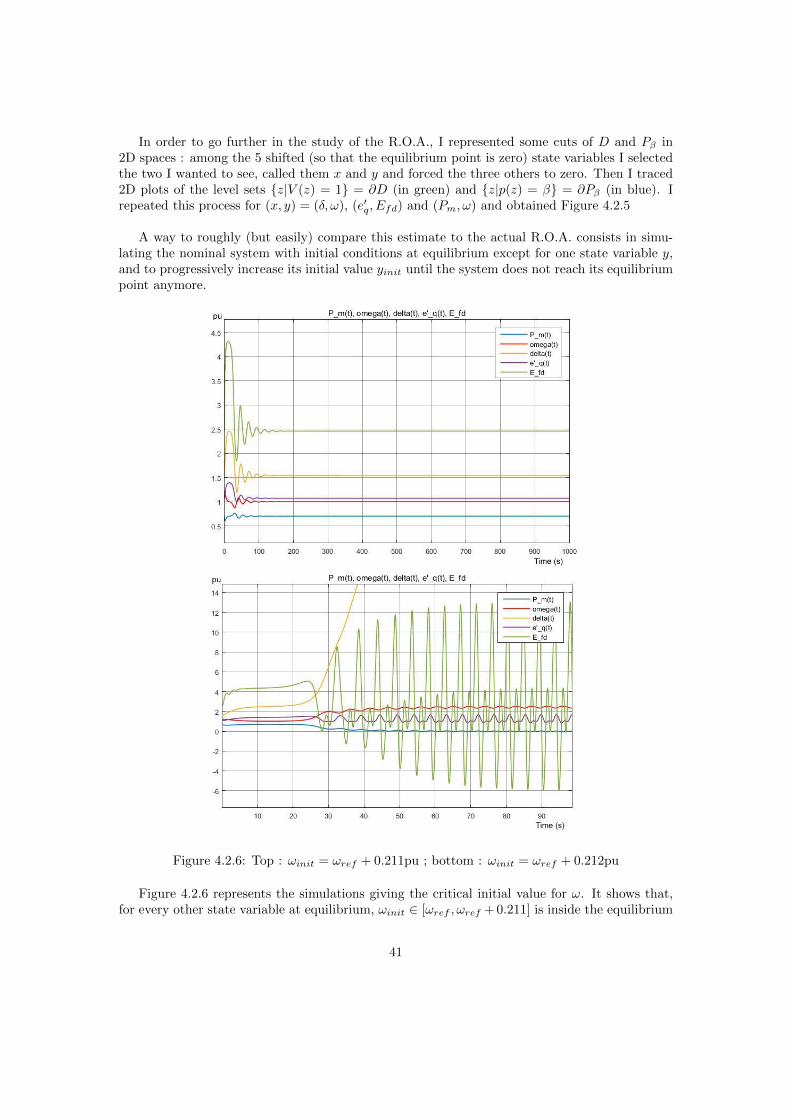
Figure 4.2.6: Top : ωinit = ωref + 0.211pu ; bottom : ωinit = ωref + 0.212pu

Figure 4.2.6 represents the simulations giving the critical initial value for ω. It shows that,for every other state variable at equilibrium, ωinit ∈ [ωref , ωref + 0.211] is inside the equilibrium

41

point’s R.O.A.In other words,

(δ, ω, e′q, Efd, Pm) ∈ R5|δ = δeq, e′q = e′eqq , Efd = Eeqfd, Pm = Pref , ωref ≤ ω ≤ ωref+0.211 ⊂ ROA.

In the case of the variable ω, Figure 4.2.5 shows that the intersection between the estimate ofthe R.O.A. and the hyper plan δ = δeq, e′q = e′eqq , Efd = Eeqfd, Pm = Pref is about [−0.2, 0.209].So considering its upper bound we only missed it by 0.02pu !

I did the same work for the other four state variables and obtained the following results :

Variable δ ω e′q Efd Pm

Actual R.O.A.’s upper bound δeq + 0.926 ωref + 0.211 e′eqq + 1.896 Eeqfd + 92.96 Pref + 3.188

R.O.A. estimate’s upper bound δeq + 0.743 ωref + 0.209 e′eqq + 0.496 Eeqfd + 14.72 Pref + 2.029

These results are quite good, especially for ω. However, the estimation of the R.O.A. forEfd is not precise at all. This explains why V surpassed 1 in the first test : the estimate of theR.O.A. is still a little too rough. Such flaw could be explained by the differences between thescales of the dynamics and the scales of p’s coefficients.

Indeed, during my internship I always kept the same polynomial p(z) = ‖z‖2 + z23 (because

it is the initial polynomial [3] used), which is equivalent to running one “outer iteration” of theinterior algorithm. The next step consists in “rescaling” p by replacing it with the functionV found in equation (4.2.6), and run again the expanding interior algorithm. This way, onecan obtain significantly better results for the estimate of the R.O.A., regardless to the system’sdynamics.

5 Personal work and contributions

My first work consisted in reading and deeply understanding the Sums of Squares theory pro-vided in [9], as well as its application to power systems dynamics as presented in [3].

Then I had to become familiar with the nominal equations of the synchronous machine in-troduced in [21], and work on a satisfying model for the short-circuit. This was quite a challengesince my only knowledge in power systems dates back to highschool and preparatory classes, butI was finally able to write the short circuit equations.

After that, my first personal contribution to the transient stability analysis problem wasto write the equations of the system under the state space form and to introduce the rightLie-Blacklund transformation so as to get a workable polynomial system.

The transformation of the angular variable had already been implemented in [3] so I justhad to tackle the change in the voltage variable, and prove that the whole was a Lie-Blacklundendogenous transformation (which had never been done).

Then, starting from Marian Anghel’s codes for the transient stability analysis of the non-regulated power system, I made some adaptations so as to derive the codes which would adressthe regulated power system.

This work proved very difficult due to the complexity of the involved Matlab codes, which Ihad to understand so as to be able to manipulate them. I received the precious help of MarianAnghel and Soumya Kundu, the authors of the codes, for this challenging and long-lasting task.

42

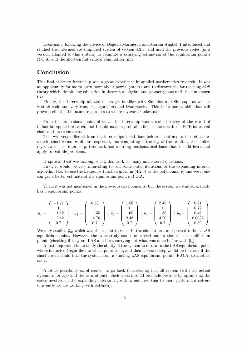
Eventually, following the advice of Bogdan Marinescu and Marian Anghel, I introduced andstudied the intermediate simplified system of section 4.2.3, and used the previous codes (in aversion adapted to this system) to compute a satisfying estimation of the equilibrium point’sR.O.A. and the short-circuit critical elimination time.

Conclusion

This End-of-Study Internship was a great experience in applied mathematics research. It wasan opportunity for me to learn more about power systems, and to discover the far-reaching SOStheory which, despite my education in theoretical algebra and geometry, was until then unknownto me.

Finally, this internship allowed me to get familiar with Simulink and Simscape as well asMatlab code and very complex algorithms and frameworks. This is for sure a skill that willprove useful for the future, regardless to where my career takes me.

From the professional point of view, this internship was a real discovery of the world ofindustrial applied research, and I could make a profitable first contact with the RTE industrialchair and its researchers.

This was very different from the internships I had done before : contrary to theoretical re-search, short-terms results are expected, and computing is the key of the results ; also, unlikemy data science internship, this work had a strong mathematical basis that I could learn andapply to real-life problems.

Despite all that was accomplished, this work let many unanswered questions.First, it would be very interesting to run some outer iterations of the expanding interior

algorithm (i.e. to use the Lyapunov function given in (4.2.6) as the polynomial p) and see if onecan get a better estimate of the equilibrium point’s R.O.A.

Then, it was not mentioned in the previous developments, but the system we studied actuallyhas 5 equilibrium points :

y1 =

−1.71

1−1.12−2.42

0.7

; y2 =

0.58

1−1.55−4.76

0.7

; y3 =

1.58

11.052.480.7

; y4 =

2.45

11.354.200.7

; y5 =

0.210.720.46

0.00320.89

We only studied y3, which was the easiest to reach in the simulations, and proved to be a LASequilibrium point. However, the same study could be carried out for the other 4 equilibriumpoints (checking if they are LAS and if so, carrying out what was done before with y3).

A first step would be to study the ability of the system to return to the LAS equilibrium pointwhere it started (regardless to which point it is), and then a second step would be to check if theshort-circuit could take the system from a starting LAS equilibrium point’s R.O.A. to anotherone’s.

Another possibility is, of course, to go back to adressing the full system (with the actualdynamics for Efd and the saturations). Such a work could be made possible by optimizing thecodes involved in the expanding interior algorithm, and resorting to more performant solvers(currently we are working with SeDuMi).

43

Furthermore, some dynamics could also be complexified : we could replace the current dy-namics for Efd and Pm by (in the Laplace domain)

Efd = Ka

(Ta +

1

s

)(Vref − V )

Pm =

(Kg +

1

Tgs

)(ωref − ω)

Indeed, the final aim of this work is to tackle far more complex transient stability problemssuch as the transient stability of an HVDC line, for example. So it is very important to find away to tackle the complexity of the systems so as to make the SOS approach useful in practice.

Actually this is currently an open question : could the SOS approach really allow engineersto carry out efficient transient stability analysis for real systems ?

Eventually, another approach to such a system would be to use the notion of flatness :

Definition A system is flat iff there exists an output set y = h(x, u, u, . . . , u(r)) such that

x = ϕ(y, y, . . . , y(q))

u = α(y, y, . . . , y(q))

Indeed, it can be prooved that the system (4.1.2) is flat. This allows to reduce it into a linearswitched system, which could be analysed using tools that differ from the SOS approach.

References

[1] Prabha Kundur. Power Systems Stability and Control. McGraw-Hill Education, 1994.

[2] Hsiao-Dong Chiang. Direct Methods for Stability Analysis of Electric Power Systems. Wiley,2011.

[3] Marian Anghel, Federico Milano, and Antonis Papachristodoulou. Algorithmic constructionof lyapunov functions for power system stability analysis. 2013.

[4] Florent Xavier. Rte : Le gestionnaire de reseau de transport et les etudes systeme (rac-cordement, reglementation,...).

[5] The rte chair website, consulted in december 2016. http://chairerte.ec-nantes.fr.

[6] The irccyn website, consulted in december 2016. http://irccyn.ec-nantes.fr.

[7] Thierry Gallay and Matteo Tacchi. Dynamique des tourbillons dans les fluides bidimension-nels.

[8] Gianluca Crippa. The flow associated to weakly differentiable vector fields. PhD thesis,Scuola Normale Superiore di Pisa, 2007.

[9] Zachary William Wloszek. Lyapunov Based Analysis and Controller Synthesis for Poly-nomial Systems using Sum-of-Squares Optimization. PhD thesis, University of California,Berkeley, 2003.

44

[10] K.P. Persidskii. On the theory of stability of solutions of differential equations. UspekhiMat. Nauk, 1:250–255, 1946.

[11] Nam Parshad. Bhatia and Giorgio P. Szego. Stability Theory of Dynamical Systems.Springer, 2002.

[12] Christopher M. Kellet. Classical converse theorems in lyapunov’s second method. Discreteand Continuous Dynamical Systems series B, 20(8), October 2015.

[13] David Hilbert. Ueber die darstellung definiter formen als summe von formenquadraten.Mathematische Annalen, 32(3):342 – 350, September 1888.

[14] Pablo A. Parrilo. Semidefinite programming relaxations for semialgebraic problems. Math-ematical Programming, Ser. B, 96(2):293–320, 2003.

[15] M. Choi, T. Lam, and B. Reznick. Sums of squares of real polynomials. In Proceedings ofSymposia in Pure Mathematics, volume 58, pages 103 – 126. 1995.

[16] Yurii Nesterov and Arkadii Nemirovskii. Interior-Point Polynomial Algorithms in ConvexProgramming. Studies in Applied and Numerical Mathematics. SIAM, 1994.

[17] Stephen Prajna, Antonis Papachristodoulou, and Pablo A. Parrilo. SOSTOOLS : Sum ofsquares optimization toolbox for Matlab. http://www.cds.caltech.edu/sostools, 2002.

[18] Stephen Prajna, Antonis Papachristodoulou, and Pablo A. Parrilo. Introducing sostools: Ageneral purpose sum of squares programming solver. In Proceedings of the Conference onDecision and Control, pages 741–746, 2002.

[19] Jos F. Sturm. Using sedumi 1.02, a matlab toolbox for optimizaton over symmetric cones.Optimization Methods and Software, 11–12:625 – 653, 1999.

[20] Jacek Bochnak, Michel Coste, and Marie-Francoise Roy. Geometrie Algebrique Reelle.Springer, 1986.

[21] Peter W. Sauer and M.A. Pai. Power System Dynamics and Stability. Prentice Hall, 1998.

[22] Michel Fliess, Jean Levine, Philippe Martin, and Pierre Rouchon. A lie-blacklund approachto equivalence and flatness of nonlinear systems. IEEE Transactions on Automatic Control,44(5):922–937, may 1999.

45