Embed Size (px)
Citation preview

Stability analysis and a priori error estimates to the third
order explicit Runge-Kutta discontinuous Galerkin Method for
scalar conservation laws
Qiang Zhang ∗ Chi-Wang Shu †
September 16, 2009
ABSTRACT. In this paper we present the analysis for the Runge-Kutta discon-tinuous Galerkin (RKDG) method to solve scalar conservation laws, where the timediscretization is the third order explicit total variation diminishing Runge–Kutta(TVDRK3) method. We use an energy technique to present the L2-norm stabilityfor scalar linear conservation laws, and obtain a priori error estimates for smoothsolutions of scalar nonlinear conservation laws. Quasi-optimal order is obtained forgeneral numerical fluxes, and optimal order is given for upwind fluxes. The theoret-ical results are obtained for piecewise polynomials with any degree k ≥ 1 under thestandard temporal-spatial CFL condition τ ≤ γh, where h and τ , respectively, arethe element length and time step, and the positive constant γ is independent of hand τ .Key words. Discontinuous Galerkin method, finite element, explicit Runge-Kuttamethod, stability analysis, error estimateAMS subject classification. 65M60, 65M12, 65M15
1 Introduction
In this paper we continue our work in [18] to consider the stability analysis and error esti-mates for the Runge-Kutta discontinuous Galerkin (RKDG) method for scalar conservationlaws
ut + ∇ · f(u) = 0, (x, t) ∈ Ω × (0, T ], (1.1a)
u(x, 0) = u0(x), x ∈ Ω, (1.1b)
where f(u) = (f1(u), . . . , fd(u)) is the given convection flux function; here x = (x1, . . . , xd) ∈Rd and u(x, t) is the unknown solution. We do not pay attention to boundary conditions inthis paper; hence the solution is considered to be either periodic or compactly supported.
∗Department of Mathematics, Nanjing University, Nanjing 210093, Jiangsu, P.R. China. E-mail:
[email protected]. The research of this author is supported by NSFC grant 10871093.†Division of Applied Mathematics, Brown University, Providence, RI 02912, USA. E-mail:
[email protected]. The research of this author is supported by NSF grant DMS-0809086 and DOE
grant DE-FG02-08ER25863.
1

For simplicity of presentation, in most cases we will only give detailed analysis for the one-dimensional case; i.e., Ω = I = (0, 1) is the unit interval. We will, however, point out anydifferences, both in the analysis and in the results, for the multidimensional cases.
The first version of the DG method was introduced in 1973 by Reed and Hill [16], inthe framework of neutron linear transport. It was later developed into RKDG methodsby Cockburn et al. [5–9] for nonlinear hyperbolic conservation laws, which use a DG dis-cretization in space and combine it with an explicit total variation diminishing Runge-Kutta(TVDRK) time-marching algorithm [17]. Later, this method was developed to solve equa-tions with higher order derivatives, see [10] and [11] for more details. It is well known thatthe DG method has strong stability and optimal accuracy to capture discontinuous jumpsand/or sharp transient layers, and it combines the advantages of finite element and finitedifference methods.
However, up until now there has been relatively few work on stability analysis and er-ror estimates for the fully discrete RKDG methods with explicit TVDRK time marching.The method of line version (continuous in time) of the DG scheme for linear equations hasbeen considered in [10, 13, 14], and has been proved to maintain good L2-norm stabilityand optimal error estimates. For nonlinear equations, there exists the well-known localentropy inequality [12] for the semi-discrete DG scheme, as well as for the fully discreteDG scheme with some special time-discretizations such as the backward Euler and Crank-Nilson algorithms. Recently, RKDG method with explicit time-discretization for nonlinearconservation laws has been analyzed in [18, 19], where the (quasi)-optimal a priori errorestimates are obtained for the second order explicit TVDRK (TVDRK2) time discretiza-tion. However, there are two limitations of the results in [18, 19]. The first is that the apriori error estimates for smooth solutions were obtained without a proof of stability forgeneral (possibly nonsmooth) solutions. In fact, up to now there has been no stabilityresult for general solutions, possibly non-smooth, for fully discrete RKDG methods withexplicit Runge-Kutta time stepping without using limiters, except for an indirect proof oflinear stability via Fourier analysis which applies only to linear partial differential equa-tions (PDEs) with uniform meshes and periodic boundary conditions. The second is thatthe error estimates in [18, 19] were obtained only for P1 elements under the standard CFLcondition τ ≤ γh, where h and τ , respectively, are the element length and time step, witha positive constant γ independent of h and τ . For Pk elements with k > 1, the resultsin [18, 19] were obtained under the much stronger time step restriction τ = o(h), which isreasonable for second order Runge-Kutta since it is linearly unconditional unstable whencoupled with DG discretization of Pk elements with k > 1 [11].
The main purpose of this paper is to overcome the two limitations above by consideringRKDG methods with a third order explicit TVDRK (TVDRK3) time discretization. Thethird order explicit RKDG algorithm is popular in practice, because it provides betterlinear stability and higher order accuracy in time. However, it is highly non-trivial toprove stability for general solutions and to obtain error estimates for smooth solutions forthe RKDG method with TVDRK3 time-marching, the techniques used in [18, 19] for theTVDRK2 time-marching must be significantly changed. We start our study with a L2-normstability analysis for linear conservation laws without restriction to the smoothness of thesolution. This result is not only important for the following error estimates for smoothsolutions, but also significant in its own right, as it provides stability assurance for the
2

fully discrete RKDG scheme for possibly discontinuous solutions. We then proceed to provequasi-optimal error estimates for general monotone fluxes and optimal error estimate forupwind numerical fluxes. All these results are obtained under the standard temporal-spatialrestriction τ ≤ γh for the piecewise polynomials with arbitrary degree k ≥ 1, where γ > 0is again a constant independent of h and τ . These results are then consistent with thewell-known practical numerical evidence and linear stability results obtained by Fourieranalysis, albeit with much more generality for non-uniform and unstructured meshes, forlinear conservation laws with variable coefficient fluxes f(u) = β(x, t)u, and for possibleh-p adaptivity. The main technical tool used in this paper is an energy analysis. The errorestimates that we obtain in this paper are for smooth solutions of nonlinear conservationlaws. A few technical details in dealing with the nonlinearity of the flux f(u) are not fullyprovided and are referred to [18].
It is well known for the semi-discrete DG scheme that the L2-norm stability resultcontains also a stability term involving the jumps of the numerical solution uh across elementinterfaces. This reflects the subtle built-in numerical dissipation mechanism of the DGmethods involving these jumps at element interfaces which allows the DG methods to bemore accurate than the standard Galerkin methods [3]. This extra stability is fully exploredin our proof of L2-norm stability of the fully discrete RKDG schemes. We will also point outthe very different stability mechanisms for the RKDG method with TVDRK2 and TVDRK3time-marchings, respectively. For both of them, the numerical viscosity provided by the DGspatial discretization is the foundation for the fully-discrete stability. However, the RKDGmethod with TVDRK3 has an additional numerical viscosity in the time direction, statedin terms of the L2-norm of a certain combination of the numerical solution in differentRunge-Kutta stages (see Section 4). This extra numerical viscosity is the key ingredientin our analysis for obtaining stability under the standard CFL condition for the RKDGmethod with arbitrary polynomial degree and TVDRK3 time-marching, while the lack of itexplains why stability under the standard CFL condition for the RKDG method can onlybe obtained for piecewise linear polynomials with TVDRK2 time-marching.
An outline of this paper is as follows. In Section 2 we present, for the equation (1.1), thefully discrete RKDG method with the explicit TVDRK3 time discretization. In Section 3 wepresent some preliminaries about the discontinuous finite element space. In Section 4 we givesome elementary properties of the DG spatial discretization, and prove the correspondingL2-norm stability, for the linear flux f(u) = βu with a constant β. Section 5 is devoted tothe error estimates for smooth solutions of nonlinear conservation laws. The main analysisis given to obtain quasi-optimal error estimates for high order piecewise polynomials witha general numerical flux, and a brief description is given to explain how to obtain optimalerror estimates for upwind numerical fluxes. Concluding remarks are given in Section 6,and Section 7 is an appendix in which we give a short analysis on the L2-norm stabilityof RKDG method with the TVDRK2 time marching, mainly to explain the very differentstability mechanisms of TVDRK2 and TVDRK3.
2 Fully discrete RKDG scheme with TVDRK3 time-marching
We follow [7] and define the RKDG method with TVDRK3 time-marching, for the problem(1.1) in one space dimension. The multidimensional case is similar. For each partition of
3

the interval I = (0, 1), xj+1/2Nj=0, we set Ij = (xj−1/2, xj+1/2), and hj = xj+1/2 − xj−1/2
for j = 1, . . . , N ; and we denote the quantities
h = max1≤j≤N
hj , and ρ = min1≤j≤N
hj . (2.1)
For simplicity of presentation we would like to assume the ratio of h over ρ is upper boundedby a fixed positive constant ν−1 when h goes to zero, namely, the computational triangula-tion is quasi-uniform with νh ≤ ρ ≤ h.
For a given time step τ (which could actually change from step to step but is taken asa constant with respect to the time level n for simplicity), the solution of the scheme isdenoted by un
h(x) = uh(x, nτ), which belongs to the finite element space
Vh = V kh = v ∈ L2(0, 1) : v|Ij
∈ Pk(Ij), j = 1, . . . , N , (2.2)
where Pk(Ij) denotes the space of polynomials in Ij of degree at most k ≥ 1. Note that thefunctions in Vh are allowed to have discontinuities across element interfaces. In this paperwe do not consider the piecewise constant, namely the k = 0 case, since in this case theconsidered DG method is just the monotone finite volume method.
In what follows, we will consider the standard L2-projection of a function p ∈ L2(0, 1)into the finite element space Vh, denoted by Php, which is defined as the unique function inVh such that
∫ 1
0(Php(x) − p(x))vh(x) dx = 0 ∀vh ∈ Vh. (2.3)
Due to the discontinuity of the finite element space, this projection is locally defined oneach element Ij .
For simplicity of presentation, we will use the following notations. Parallel to the dis-continuous finite element space Vh, we denote the broken Sobolev space as follows
H1,h(Th) = φ ∈ L2(I) : φ|Ij∈ H1(Ij), j = 1, 2, . . . , N , (2.4)
where Th is the union of all cells Ij in the partition. For any function p ∈ H1,h(Th), at eachelement boundary point there are two limits from different directions, namely, the left-valuep− and the right-value p+. Furthermore, the jump and the mean at the element boundarypoint, respectively, are denoted by [[p]] = p+ − p−, and p = 1
2(p+ + p−).Following [18], we would like to give an abbreviate notation for the DG spatial operator.
For any functions p and q in H1,h(Th), on each element Ij we define
Hj(p, q) =
∫
Ij
f(p)qx(x) dx− f(p)j+ 1
2
q(x−j+ 1
2
) + f(p)j− 1
2
q(x+j− 1
2
), (2.5)
where f(p) ≡ f(p−, p+) is a given monotone numerical flux that depends on the two values ofthe function p at the element interface point. The numerical flux f(a, b) is locally Lipschitzcontinuous with regard to both arguments, and is consistent with the flux f(p), namely,f(p, p) = f(p). Furthermore, it is a nondecreasing function of its first argument and anonincreasing function of its second argument. The best-known examples of monotonenumerical fluxes are the Godunov flux, the Engquist-Osher flux, the Lax-Friedrichs flux,
4

etc. Some of these monotone fluxes (e.g. the Godunov flux and the Engquist-Osher flux)are upwind fluxes, namely f(a, b) = f(a) if f ′(u) ≥ 0 when u is between a and b, andf(a, b) = f(b) if f ′(u) ≤ 0 when u is between a and b. For more details, see, for example, [15].
There are three steps in the construction of a RKDG scheme. First, we multiply a testfunction vh on both sides of the equation (1.1a), and integrate them by parts in each elementIj. Next, we define the suitable numerical flux at the element interface point, and get thesemi-discrete DG method. Finally we adopt the Runge-Kutta type time discretization. Formore details, see, for example, [7, 11].
In this paper the considered scheme is the fully discrete RKDG method coupled withthe explicit TVDRK3 time marching. First, we set the initial value u0
h = Phu0(x). Thenfor each n ≥ 0, the approximate solution from the time nτ to the next time (n + 1)τ isdefined as follows: find un,1
h , un,2h and un+1
h in the finite element space Vh, such that for anyvh ≡ vh(x) ∈ Vh and 1 ≤ j ≤ N , on each element Ij there hold
∫
Ij
un,1h vh dx =
∫
Ij
unhvh dx+ τHj(u
nh, vh), (2.6a)
∫
Ij
un,2h vh dx =
3
4
∫
Ij
unhvh dx+
1
4
∫
Ij
un,1h vh dx+
τ
4Hj(u
n,1h , vh), (2.6b)
∫
Ij
un+1h vh dx =
1
3
∫
Ij
unhvh dx+
2
3
∫
Ij
un,2h vh dx+
2τ
3Hj(u
n,2h , vh). (2.6c)
This is an explicit time-marching method when a local orthogonal basis is chosen for poly-nomials on Ij or when a small local mass matrix on Ij is inverted.
3 Preliminaries
In this section we would like to present some properties of the discontinuous finite elementspace Vh, which will be used in the stability analysis and error estimates. In this paperwe use C (possibly with subscripts) to denote a positive constant depending solely on theexact solution, which may have a different value in each occurrence.
The usual notation of norms in Sobolev spaces will be used. For any integer s ≥ 0, letHs(Ω) represent the well-known Sobolev space equipped with the norm ‖·‖s, which consistsof functions with (distributional) derivatives of order not greater than s in L2(Ω). Next, letthe scalar inner product on L2(Ω) be denoted by (·, ·)Ω, and the associated norm by ‖ · ‖Ω.Furthermore, let ‖ · ‖∞,Ω represent the norm on L∞(Ω). If Ω = I we omit this subscript.See Adams [1] for more details.
3.1 Projections to the finite element space
As a standard trick in DG analysis, two types of projections, denoted by Qhp(·, t), are usedin this paper. One is the standard L2-projection Ph, and the other is the Gauss-Radauprojection R±
h . They will be used to get error estimates of the quasi-optimal and optimalorder, respectively.
The standard L2-projection Ph has been defined in Section 2; see (2.3). In what followswe define two kinds of the Gauss-Radau projection R±
h , corresponding to the positive direc-tion and the negative direction of the x-axis, respectively. For any function p ∈ H 1(0, 1),
5

R±h p is defined element by element as the unique function in Vh, such that for any 1 ≤ j ≤ N ,
∫
Ij
R±h p(x)vh(x) dx =
∫
Ij
p(x)vh(x) dx, ∀ vh(x) ∈ Pk−1(Ij), (3.1)
and the exact collocation at one endpoint, namely (R+h p)
−j+1/2
= p−j+1/2
for the positive
projection R+h , and (R−
h p)+j−1/2 = p+
j−1/2 for the negative projection R−h , respectively.
3.2 Projection properties
Denote by η = p(x) − Qhp(x) the projection error. By a standard scaling argument [2, 14],it is easy to obtain, for both projections, that,
‖η‖ + h‖ηx‖ + h1/2‖η‖Γh≤ Chk+1 (3.2)
if p(x) is smooth enough, where C is a positive constant independent of h. This constantdepends on ‖p‖k+1 for the standard L2-projection, and on ‖p‖k+2 for the Gauss-Radauprojection. Here Γh is the union of all element interface points, and the L2-norm on Γh isdefined by
‖η‖Γh=
[
∑
1≤j≤N
((η+j+ 1
2
)2 + (η−j+ 1
2
)2)]1/2
. (3.3)
It is worthy to point out that on each element interface point the Gauss-Radau projectionR±
h has the estimate (3.2), and furthermore, it is the exact collocation along one of the twodirections. Namely η−j+1/2 = 0 for R+
h , and η+j+1/2 = 0 for R−
h , respectively. This propertyis very helpful to obtain the optimal error estimates.
3.3 Inverse properties
Finally, we list some inverse properties of the finite element space Vh. For any vh ∈ Vh,there exist positive constants µi, (i = 1, 2, 3), independent of vh and h, such that
(i) ‖vh,x‖ ≤ µ1h−1‖vh‖; (ii) ‖vh‖Γh
≤ µ2h−1/2‖vh‖; (iii) ‖vh‖∞ ≤ µ3h
−1/2‖vh‖.
For more details of these inverse properties, we refer the reader to [2]. The inverse inequality(iii) will not be used in the analysis for linear conservation laws. In the following we willdenote µ = maxµ1, (µ2)
2, which increases with the degree of polynomials.
4 Stability analysis for the linear conservation law
In this section we are going to obtain the L2-norm stability for the fully discrete RKDGmethod with TVDRK3 time-marching, where f(u) = βu with the given constant β. Theanalysis in this section forms the foundation of all results in this paper.
6

4.1 DG spatial discretization for the linear flux
For the linear flux f(u) = βu, the DG spatial discrete operator is given as
Hj(φ, ψ) =
∫
Ij
βφψxdx− f(φ)j+1/2ψ−j+1/2 + f(φ)j−1/2ψ
+j−1/2, (4.1)
for any φ and ψ in H1,h(Th). Note that in this case, all the monotone numerical fluxesmentioned in Section 2 and used in practice coincide and are equal to an upwind numericalflux
f(φ) = f(φ−, φ+) =
βφ−, if β > 0βφ+, if β < 0.
(4.2)
It is convenient to consider the summation of (4.1) over all j, which is denoted byH(φ, ψ). The periodic boundary condition yields that
H(φ, ψ) =∑
1≤j≤N
Hj(φ, ψ) =∑
1≤j≤N
[
f(φ)j+1/2[[ψ]]j+1/2 +
∫
Ij
βφψxdx]
. (4.3)
Below we present some elementary properties of this bilinear operator.The next lemma describes the continuity in the L2-norm of this operator, with the
bounding constant depending on the spatial mesh size h.
Lemma 4.1 For any ψ and φ in Vh, we have |H(φ, ψ)| ≤ (√
2 + 1)|β|µh−1‖φ‖‖ψ‖.
Proof. This proof is straightforward. First we point out that∑
1≤j≤N
[[ψ]]2j+ 1
2
≤ 2∑
1≤j≤N
[
(ψ+j+ 1
2
)2 + (ψ+j+ 1
2
)2]
= 2‖ψ‖2Γh, (4.4)
and∑
1≤j≤N |f(φ)j+ 1
2
|2 ≤ |β|2‖φ‖2Γh
owing to the definition (4.2). By using Schwartz
inequality, together with the inverse properties (i) and (ii), we have
|H(φ, ψ)| ≤∣
∣
∣
∫
Iβφψx dx
∣
∣
∣+
∑
1≤j≤N
|f(φ)j+ 1
2
| · |[[ψ]]j+ 1
2
|
≤ |β|‖φ‖‖ψx‖ +√
2|β|‖φ‖Γh‖ψ‖Γh
≤µ1h−1|β|‖φ‖‖ψ‖ +
√2(µ2)
2h−1|β|‖φ‖‖ψ‖≤ (
√2 + 1)|β|µh−1‖φ‖‖ψ‖,
since µ = maxµ1, (µ2)2. This completes the proof.
The next lemma describes the approximate anti-symmetry property of the operatorH(ψ, φ), which helps us to obtain the L2-norm stability under the standard temporal-spatialCFL condition. It also implies the negative semi-definiteness of this operator.
Lemma 4.2 For any φ and ψ in H1,h(Th), we have
H(ψ, φ) + H(φ, ψ) = −∑
1≤j≤N
|β|[[φ]]j+ 1
2
· [[ψ]]j+ 1
2
, (4.5a)
H(φ, φ) = − 1
2
∑
1≤j≤N
|β|[[φ]]2j+1/2. (4.5b)
7

Proof. Obviously, (4.5b) is a corollary of the identity (4.5a), if ψ = φ. So we only prove(4.5a) below. In fact, from (4.3) we can easily work out the details as follows
H(ψ, φ) + H(φ, ψ)
=∑
1≤j≤N
[
f(φ)j+1/2[[ψ]]j+1/2 + f(ψ)j+1/2[[φ]]j+1/2
]
+∑
1≤j≤N
∫
Ij
β(φψ)x dx
=∑
1≤j≤N
[
f(φ)j+1/2[[ψ]]j+1/2 + f(ψ)j+1/2[[φ]]j+1/2 − β[[φψ]]j+1/2
]
=∑
1≤j≤N
[
(f(φ)j+1/2 − βφ+j+ 1
2
)[[ψ]]j+1/2 + (f(ψ)j+1/2 − βψ−
j+ 1
2
)[[φ]]j+1/2
]
, (4.6)
where we have used the periodic boundary condition for the second equality, and used[[φψ]] = φ+[[ψ]] + ψ−[[φ]] for the last equality.
Noticing the definition of the numerical flux, (4.2), we get that
f(φ) − βφ+ =
−β[[φ]], if β > 00, if β < 0.
, f(ψ) − βψ− =
0, if β > 0β[[ψ]], if β < 0.
Hence we clearly get (4.5a) from (4.6).
4.2 Time-marching in TVDRK3
In the RKDG method with TVDRK3 time-marching, for linear conservation laws, theapproximate time derivatives up to the third order at time t = tn are proportional tocertain linear combinations of the numerical solution in different Runge-Kutta stages. Tobe more specific, we denote
Dn1 = un,1
h − unh, Dn
2 = 2un,2h − un,1
h − unh, Dn
3 = un+1h − 2un,2
h + unh, (4.7)
and set up the following lemma, where the spatial DG operator H(·, ·) can be considered asthe discrete approximation of the time derivative because of the PDE.
Lemma 4.3 For the fully discrete DG method (2.6) with the explicit TVDRK3 timemarching, we have the following identities
(Dn1 , vh) = τH(un
h, vh), ∀ vh ∈ Vh; (4.8a)
(Dn2 , vh) =
τ
2H(Dn
1 , vh), ∀ vh ∈ Vh; (4.8b)
(Dn3 , vh) =
τ
3H(Dn
2 , vh), ∀ vh ∈ Vh. (4.8c)
Proof. It is straightforward to get (4.8a) by summing (2.6a) over all elements. It isalso straightforward to get (4.8b) by subtracting half of (2.6a) from twice of (2.6b), andsumming over all elements.
To prove (4.8c), we first substitute (2.6a) into (2.6b). Summing it over all elements gives(un,2
h − unh, vh) = τ
4H(un,1h + un
h, vh), for any vh ∈ Vh. Subtracting 43 of this equality from
8
(2.6c) yields,
(Dn3 , vh) =
(
un+1h − 1
3un
h − 2
3un,2
h , vh
)
− 4
3
(
un,2h − un
h, vh
)
=2τ
3H(un,2
h , vh) − τ
3H(un,1
h + unh, vh)
=τ
3H(2un,2
h − un,1h − un
h, vh) =τ
3H(Dn
2 , vh), ∀ vh ∈ Vh,
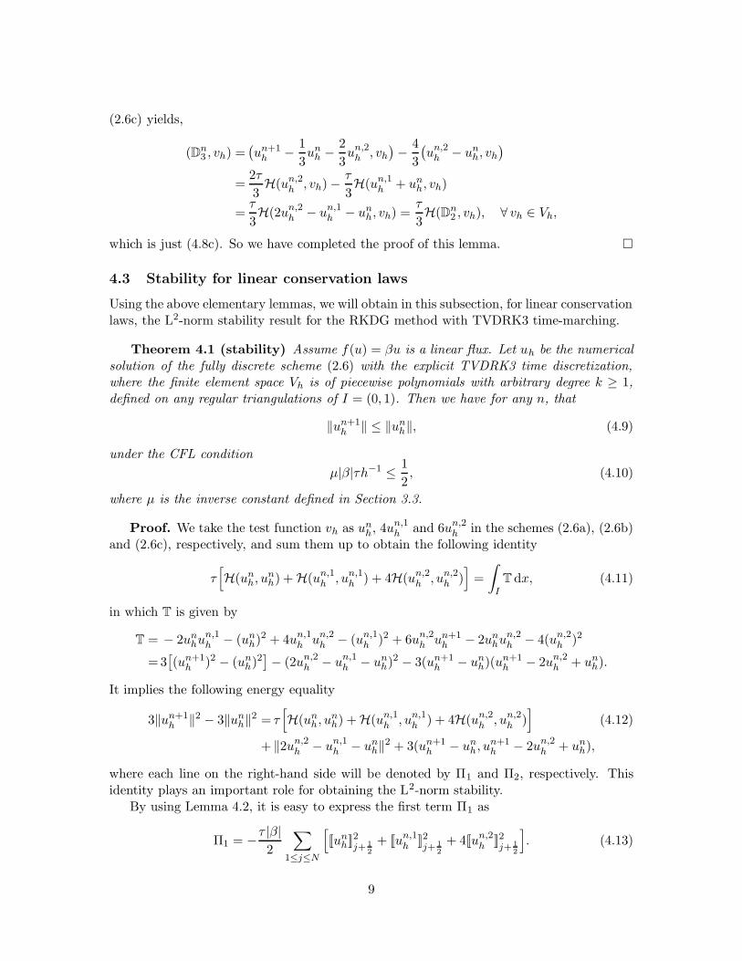
which is just (4.8c). So we have completed the proof of this lemma.
4.3 Stability for linear conservation laws
Using the above elementary lemmas, we will obtain in this subsection, for linear conservationlaws, the L2-norm stability result for the RKDG method with TVDRK3 time-marching.
Theorem 4.1 (stability) Assume f(u) = βu is a linear flux. Let uh be the numericalsolution of the fully discrete scheme (2.6) with the explicit TVDRK3 time discretization,where the finite element space Vh is of piecewise polynomials with arbitrary degree k ≥ 1,defined on any regular triangulations of I = (0, 1). Then we have for any n, that
‖un+1h ‖ ≤ ‖un
h‖, (4.9)
under the CFL condition
µ|β|τh−1 ≤ 1
2, (4.10)
where µ is the inverse constant defined in Section 3.3.
Proof. We take the test function vh as unh, 4un,1
h and 6un,2h in the schemes (2.6a), (2.6b)
and (2.6c), respectively, and sum them up to obtain the following identity
τ[
H(unh, u
nh) + H(un,1
h , un,1h ) + 4H(un,2
h , un,2h )
]
=
∫
IT dx, (4.11)
in which T is given by
T = − 2unhu
n,1h − (un
h)2 + 4un,1h un,2
h − (un,1h )2 + 6un,2
h un+1h − 2un
hun,2h − 4(un,2
h )2
=3[
(un+1h )2 − (un
h)2]
− (2un,2h − un,1
h − unh)2 − 3(un+1
h − unh)(un+1
h − 2un,2h + un
h).
It implies the following energy equality
3‖un+1h ‖2 − 3‖un
h‖2 = τ[
H(unh, u
nh) + H(un,1
h , un,1h ) + 4H(un,2
h , un,2h )
]
(4.12)
+ ‖2un,2h − un,1
h − unh‖2 + 3(un+1
h − unh, u
n+1h − 2un,2
h + unh),
where each line on the right-hand side will be denoted by Π1 and Π2, respectively. Thisidentity plays an important role for obtaining the L2-norm stability.
By using Lemma 4.2, it is easy to express the first term Π1 as
Π1 = −τ |β|2
∑
1≤j≤N
[
[[unh]]2
j+ 1
2
+ [[un,1h ]]2
j+ 1
2
+ 4[[un,2h ]]2
j+ 1
2
]
. (4.13)
9

However, we have to cope with the second term Π2 carefully, in order to show that Π2 doesnot exceed the absolute value of Π1 under a suitable CFL condition.
To do that, we express Π2 by Dni , i = 1, 2, 3. Since un+1
h − unh = Dn
1 + Dn2 + Dn
3 , thereholds the following equivalent representation
Π2 = (Dn2 ,D
n2 ) + 3(Dn
3 ,Dn1 ) + 3(Dn
3 ,Dn2 ) + 3(Dn
3 ,Dn3 ) = Λ1 + Λ2 + Λ3 + Λ4. (4.14)
Below we will estimate each term in (4.14) separately.First we estimate the sum of Λ1 and Λ2, which will help us to get rid of the negative
contribution from the integration in each element. The estimate reads
Λ1 + Λ2 = − (Dn2 ,D
n2 ) + 2(Dn
2 ,Dn2 ) + 3(Dn
3 ,Dn1 )
= − ‖Dn2‖2 + τH(Dn
1 ,Dn2 ) + τH(Dn
2 ,Dn1 )
= − ‖Dn2‖2 − τ
∑
1≤j≤N
|β|[[Dn1 ]]j+ 1
2
[[Dn2 ]]j+ 1
2
≤ − ‖Dn2‖2 +
τ
4
∑
1≤j≤N
|β|[[Dn1 ]]2
j+ 1
2
+ τ∑
1≤j≤N
|β|[[Dn2 ]]2
j+ 1
2
(4.15)
where for the second equality we have used the identities (4.8b) and (4.8c) in Lemma 4.3,with different test functions vh = Dn
2 and vh = Dn1 , respectively; the third equality is a
direct application of (4.5a) in Lemma 4.2; and the last inequality is a simple application ofYoung’s inequality.
Identities (4.8c) and (4.5b), in Lemma 4.3 and Lemma 4.2, respectively, yield the esti-mate to the third term Λ3. It reads
Λ3 = 3(Dn3 ,D
n2 ) = τH(Dn
2 ,Dn2 ) = −τ
2
∑
1≤j≤N
|β|[[Dn2 ]]2
j+ 1
2
. (4.16)
To estimate the last term Λ4, we use again identity (4.8c) in Lemma 4.3. It follows fromLemma 4.1 that
‖Dn3‖2 = (Dn
3 ,Dn3 ) =
τ
3H(Dn
2 ,Dn3 ) ≤
√2 + 1
3|β|µτh−1‖Dn
2‖‖Dn3‖.
Denote = (2√
2 + 3)/3 and λmax = µ|β|τh−1. Consequently, the above inequality implies
Λ4 = 3‖Dn3‖2 ≤ 2
√2 + 3
3[µ|β|τh−1]2‖Dn
2‖2 ≡ λ2max‖Dn
2‖2. (4.17)
Now we collect the estimates above from (4.15) to (4.17), and get that
Π2 ≤ τ
4
∑
1≤j≤N
|β|[[Dn1 ]]2
j+ 1
2
+τ
2
∑
1≤j≤N
|β|[[Dn2 ]]2
j+ 1
2
− (1 − λ2max)‖Dn
2‖2
≤ τ
2
∑
1≤j≤N
|β|[
[[unh]]2
j+ 1
2
+ [[un,1h ]]2
j+ 1
2
]
+ τ |β|‖Dn2‖2
Γh− (1 − λ2
max)‖Dn2‖2
≤ τ
2
∑
1≤j≤N
|β|[
[[unh]]2
j+ 1
2
+ [[un,1h ]]2
j+ 1
2
]
+ |β|(µ2)2τh−1‖Dn
2‖2 − (1 − λ2max)‖Dn
2‖2
≤ τ
2
∑
1≤j≤N
|β|[
[[unh]]2
j+ 1
2
+ [[un,1h ]]2
j+ 1
2
]
− (1 − λ2max − λmax)‖Dn
2‖2,
10

where we have used the inequality (4.4) for the second inequality, and the inverse inequality(ii) for the third inequality. The last inequality is obvious since (µ2)
2 ≤ µ, see Section 3.3.We now substitute the estimates about Π1 and Π2 into the energy identity (4.12). Note
that the temporal-spatial restriction (4.10) implies 1 − λ2max − λmax > 0. Finally, under
this CFL condition, we obtain the following inequality
3‖un+1h ‖2 − 3‖un
h‖2 + 2τ∑
1≤j≤N
|β|[[un,2h ]]2
j+ 1
2
≤ 0. (4.18)
This finishes the proof.
Remark 4.1. We have proved that the fully discrete RKDG scheme with TVDRK3time marching does not destroy the L2-norm stability of the semi-discrete DG method. Theproof depends strongly on the combination of numerical solutions in different stages, andthe approximate anti-symmetry property (4.5a) in Lemma 4.2.
For the RKDG scheme, the TVDRK3 time marching has a different mechanism to ensurethe L2-norm stability, in comparison with TVDRK2. For both types of time-marching,the square of jumps over all element boundary points plays an important role. However,TVDRK3 has an additional numerical stability in terms of the L2-norm of Dn
2 , which islacking for TVDRK2. This is the reason that stability for RKDG with TVDRK2 canbe proved only for piecewise linear polynomials, while with TVDRK3 stability holds forpiecewise polynomials with arbitrary degree. In order to highlight this point, we providethe L2-norm stability analysis for the RKDG method with TVDRK2 in the appendix.
Remark 4.2. Even though we proved Theorem 4.1 only for the specific third orderTVD Runge-Kutta time discretization (2.6), the stability result actually holds for all threestage, third order Runge-Kutta time discretization. This is because for linear, constantcoefficient ordinary differential equations, all three stage, third order Runge-Kutta methodsare equivalent.
Remark 4.3. The analysis above and the stability results can be easily generalized tomulti-dimensional linear conservation laws, including those with varying coefficients β =β(x), on arbitrary regular triangulations with either periodic or other well-posed boundaryconditions. However, it does not seem easy to extend the analysis to nonlinear flux functionsf(u). One technical difficulty is that the anti-symmetry property in Lemma 4.2 does nothold for the nonlinear case.
5 A priori error estimate
In this section we carry out an a priori error estimate for the fully-discrete RKDG schemewith the explicit TVDRK3 time marching for smooth solutions.
We assume the exact solution of the conservation law (1.1) is smooth enough, for ex-ample, ‖u‖k+1 and ‖ut‖k+1 are bounded uniformly for any time t ∈ [0, T ]. Moreover, uitself and its spatial derivatives up to the second order are all continuous in I = (0, 1).For some results, additional smoothness properties may be needed. For example, to obtainoptimal error estimates, we assume ‖u‖k+2 and ‖ut‖k+2 are bounded uniformly for any timet ∈ [0, T ].
11

Furthermore, the nonlinear flux function f(u) is assumed to be smooth enough, alsof(u) and its derivatives up to the third order are all bounded on R. For a given initialcondition, this assumption is reasonable with the original or a suitably modified flux f(u),see [18] for more details. To emphasize the nonlinearity of f(u), we use C? to denote anonnegative constant depending solely on the maximum of |f ′′(u)|. Remark that C? = 0for a linear flux f(u) = βu.
We would like to present the error estimate result here, and prove it by the energytechnique in the next subsections. The main work is to cope with the accumulation of theerror from the time discretization. To deal with the nonlinearity of f(u), Taylor expansionand an a priori assumption are used.
Theorem 5.1 (error estimate) Let uh be the numerical solution of the fully discretescheme (2.6) with the explicit TVDRK3 time marching, where the finite element space Vh isof piecewise polynomials with arbitrary degree k ≥ 1, defined on any regular triangulationsof I = (0, 1). Let u be the exact solution of problem (1.1), where the flux f(u) is smoothenough. If u is sufficiently smooth with bounded derivatives, then there holds the followingerror estimate
maxnτ≤T
‖u(tn) − unh‖ ≤ C(hk+σ + τ3), (5.1)
under a CFL condition τ ≤ γh with a fixed CFL constant γ > 0, where σ = 12 for a general
monotone numerical flux, and σ = 1 for a upwind numerical flux. Here C is a positiveconstant independent of h, τ , and the approximate solution uh.
5.1 Error representation
Following [18], reference functions are defined in parallel to the Runge-Kutta time discretiza-tion stages for the exact solution of the conservation law (1.1). Let u(0)(x, t) = u(x, t), and
u(1)(x, t) = u(0)(x, t) − τ [f(u(0)(x, t))]x, (5.2a)
u(2)(x, t) =3
4u(0)(x, t) +
1
4u(1)(x, t) − 1
4τ [f(u(1)(x, t))]x. (5.2b)
Denote un,] = u(])(x, tn), for any time level n and ] = 0, 1, 2.
The error at each stage is denoted by en,] = un,] − un,]h , for any n and inner stage
] = 0, 1, 2, where un,0h = un
h. As the usual treatment in a finite element analysis, we dividethe error into two parts, en,] = ξn,] − ηn,], with
ξn,] = Qhun,] − un,]
h , ηn,] = Qhun,] − un,], (5.3)
where Qh is a given projection operator. Here ξn,] ∈ Vh would require a careful estimatein the next subsections, while ηn,] is the approximation error depending on the specificprojection. For simplicity we denote en = en,0 and ξn = ξn,0 below.
The projection operator Qh is taken for different purposes. To obtain quasi-optimal errorestimates for general monotone fluxes, it is enough to take Qh as the standard L2-projectionPh. However, to obtain an optimal error estimate we would like to follow a standard trickin DG analysis and take Qh as the generalized Gauss-Radau projection Rh. For any given
12

function p(·, tn) at the time level t = tn, the projection operator Rh ≡ Rnh actually depends
on the exact solution u(x, tn), which is defined in each element as
Rh =
R+h , if f ′(un) > 0 in the element Ij ,
R−h , if f ′(un) < 0 in the element Ij ,
Ph, if f ′(un) changes its sign on the element Ij .(5.4)
For a linear flux f(u) = βu, this generalized Gauss-Radau projection Rh solely depends onthe sign of β, namely, Rh = R+
h if β > 0, otherwise Rh = R−h if β < 0.
At the end of this subsection we present some estimates for the projection error ηn,].Since u is assumed to be smooth enough, from (3.2) there holds
‖ηn,]‖ + h‖ηn,]x ‖ + h1/2‖ηn,]‖Γh
≤ C1hk+1, ∀n : nτ ≤ T ; (5.5a)
Then it follows from the Sobolev’s inequality that
‖ηn,]‖∞ ≤ C2hk+ 1
2 , ∀n : nτ ≤ T. (5.5b)
By n = d3η
n+1+d2ηn,2+d1η
n,1+d0ηn, we denote a linear combination of errors in different
stages, where di, (i = 0, 1, 2, 3), are any four constants restricted by d0 + d1 + d2 + d3 = 0.Note Qh is linear in time for both the standard L2-projection and the generalized Gauss-Radau projection (5.4), since the considered exact solution is smooth and the characteristicswill not intersect with each other; see [18] for more details. Thus we also have
‖ n‖ + h1/2‖ n‖Γh≤ C3h
k+1τ, ∀n : nτ ≤ T ; (5.5c)
when ut is smooth enough. Here C1, C2 and C3 are positive constants independent of n, h,and τ .
5.2 The error equation and the energy equation
To obtain the error equation for different stages of the Runge-Kutta time-marching, we firstpresent the local truncation error in time for the reference functions.
Lemma 5.1 If u(·, t) ∈ C4[0, T ], then we have
u(x, t+ τ) =1
3u(0)(x, t) +
2
3u(2)(x, t) − 2
3τ [f(u(2)(x, t))]x + E(x, t), (5.6)
where E(x, t) is the local truncation error in time, and ‖E(x, t)‖ = O(τ 4) uniformly for anytime t ∈ [0, T ].
Proof. Obviously this lemma is a direct application of the explicit TVDRK3 time-marching for the generalized “ordinary differential equation” ut = −[f(u)]x.
We multiply the test function vh ∈ Vh on both sides of (5.2a), (5.2b) and (5.6), respec-tively. Let t = tn and integrate the above equations by parts. Since u is assumed to besmooth enough, the reference functions un,] are all continuous in I = (0, 1). Thus the exactflux is equal to the numerical flux at each element boundary point. The process above then
13

yields a set of equalities similar to the scheme (2.6). Subtracting these equalities from thescheme (2.6) gives the error equations for ξn,] as follows: for any test function vh ∈ Vh and1 ≤ j ≤ N , there holds
∫
Ij
ξn,1vh dx =
∫
Ij
ξnvh dx+ τJj(vh), (5.7a)
∫
Ij
ξn,2vh dx =3
4
∫
Ij
ξnvh dx+1
4
∫
Ij
ξn,1vh dx+τ
4Kj(vh), (5.7b)
∫
Ij
ξn+1vh dx =1
3
∫
Ij
ξnvh dx+2
3
∫
Ij
ξn,2vh dx+2τ
3Lj(vh). (5.7c)
These equalities have the same form as the scheme (2.6), with the spatial discrete DG
operator Hj(un,]h , vh), ] = 0, 1, 2, respectively, replaced by three error operators
Jj(vh) =
∫
Ij
1
τ(ηn,1 − ηn)vh dx+ Dj(u
n, unh, vh), (5.8a)
Kj(vh) =
∫
Ij
1
τ(4ηn,2 − 3ηn − ηn,1)vh dx+ Dj(u
n,1, un,1h , vh), (5.8b)
Lj(vh) =
∫
Ij
1
2τ
[
3ηn+1 − ηn − 2ηn,2 + 3E(x, tn)]
vh dx+ Dj(un,2, un,2
h , vh). (5.8c)
The integrals in (5.8) are denoted by J tmj (vh),Ktm
j (vh) and Ltmj (vh), respectively, and
Dj(a, b, vh) = Hj(a, vh) − Hj(b, vh). Furthermore, we would remove the subscript j todenote the sum of the operator over all elements.
By taking the test function vh = ξn, 4ξn,1 and 6ξn,2 in the error equations (5.7a), (5.7b)and (5.7c), respectively, we get the energy equation for ξn in the form
3‖ξn+1‖2 − 3‖ξn‖2 = τ[
J (ξn) + K(ξn,1) + 4L(ξn,2)]
(5.9)
+ ‖2ξn,2 − ξn,1 − ξn‖2 + 3(ξn+1 − ξn, ξn+1 − 2ξn,2 + ξn),
where each line on the right-hand side will be denoted by Π′1 and Π′
2, respectively.In the next subsection we will estimate Π′
1 and Π′2 separately. The analysis follows the
same line as that in the stability analysis. When the modification from the stability analysisis trivial, we will only present the result without the detailed proof.
5.3 Estimate for the right-hand side of (5.9)
In this subsection we estimate Π′1 and Π′
2 for a general monotone numerical flux, to obtain aquasi-optimal error estimate. It is then enough to use the standard L2-projection, Qh = Ph.However, this analysis can be suitably modified to treat a upwind numerical flux for anoptimal error estimate; see Section 5.5.
5.3.1 An important quantity of viscosity
For a general monotone numerical flux f(u−, u+) consistent with f(u), we follow [18] andintroduce an important quantity α(f ; p) to measure the viscosity provided by the numerical
14

flux. For any piecewise smooth function p ∈ H1,h(Th), on each element boundary point wedefine it as
α(f ; p) ≡ α(f ; p−, p+) ≡
[[p]]−1(f(p) − f(p−, p+)) if [[p]] 6= 0,
|f ′(p)| if [[p]] = 0.(5.10)
For this quantity we have the following lemma.
Lemma 5.2 α(f ; p) is nonnegative, and is bounded for any (p−, p+) ∈ R2. Moreover,this quantity is equivalent to 1
2 |f ′(p)|, in the sense that there exists a constant C? ≥ 0depending solely on the maximum of |f ′′(u)|, such that
α(f ; p) − C?|[[p]]| ≤1
2
∣
∣f ′(p)∣
∣ ≤ α(f ; p) + C?|[[p]]|. (5.11)
Proof. The conclusions are cited from [18], except the left inequality in (5.11). Thisinequality comes from the monotone property, with respect to each argument, of the nu-merical flux f(p−, p+). For simplicity, we assume p+ ≥ p− as an example. If f ′(p) ≥ 0,then we use the consistency property of f and a Taylor expansion to conclude
α(f ; p) ≤ [[p]]−1(f(p) − f(p+, p+)) =1
2f ′(p) + O(|[[p]]|); (5.12)
If f ′(p) < 0, we also have
α(f ; p) ≤ [[p]]−1(f(p) − f(p−, p−)) = −1
2f ′(p) + O(|[[p]]|), (5.13)
where −f ′(p) = |f ′(p)|. Remark that O(|[[p]]|) ≤ C?|[[p]]|, so we get the left inequalityin (5.11). This completes the proof of this lemma.
Below we will use some compact notations with regard to the quantity α(f ; p), as wehave done in [18]. For any functions q1 and q2, we denote
α(f ; p)[[q1]][[q2]] =∑
1≤j≤N
α(f ; p)j+ 1
2
[[q1]]j+ 1
2
[[q2]]j+ 1
2
. (5.14)
If q1 = q2, we use the simplified notation α(f ; p)[[q1]]2. Similarly we also use |f ′(p)|[[q]]2 to
denote the sum of itself over all element interface points.
5.3.2 Some basic estimates
The main term for the error operators (5.8) is D(un,], un,]h , vh). Here and below we drop the
superscripts and denote this term by D(u, uh, vh) with u = un,] and uh = un,]h , if there is
no confusion.We present some basic estimates to D(u, uh, vh) for any test function vh, and furthermore
for the specific test function ξ = ξn,]. For writing convenience, we denote
Tint(e) = f(u) − f(uh) − f ′(u)e, (5.15a)
Tbry(e) = f(u) − f(uh) − f ′(u)e, (5.15b)
15

to represent the nonlinear part of f(u) together with the central numerical flux, where uhis referred as the reference value at each element interface. For a linear flux f(u) = βu,these terms in (5.15) are zero.
We separate the operator D(u, uh, vh) into three parts
D(u, uh, vh) = Hlin(f ′(u); e, vh) + Hnls(e; vh) + V(uh; vh), (5.16)
in which the three parts are termed as the linear part, the nonlinear part and the viscositypart, respectively. They are given for any w and v as follows:
Hlin(f ′(u);w, v) =∑
1≤j≤N
[
(f ′(u)w[[v]])j+ 1
2
+
∫
Ij
f ′(u)wvx dx]
, (5.17a)
Hnls(e; v) =∑
1≤j≤N
[
(Tbry(e)[[v]])j+ 1
2
+
∫
Ij
Tint(e)vx dx]
, (5.17b)
V(uh; v) =∑
1≤j≤N
(f(uh) − f(uh))j+ 1
2
[[v]]j+ 1
2
. (5.17c)
Note that only Hlin(f ′(u);w, v) is a bilinear operator with respect to w and v. Hnls(e; v)and V(uh; v) are linear operators with respect to v.
The next three lemmas are given for different parts. One can see that numerical stabilityis not provided by the linear part (with the central reference value), but by the viscositypart. The nonlinear part does not affect the order of the error, and it disappears for thelinear flux f(u) = βu.
Lemma 5.3 Denote Smax = maxs∈R |f ′(s)|. Then we have
|Hlin(f ′(u); ξ, vh)| ≤ 2Smaxµh−1‖ξ‖‖vh‖, ∀ vh ∈ Vh; (5.18a)
|Hlin(f ′(u); ξ, ξ)| ≤C?‖ξ‖2, (5.18b)
where C? ≥ 0 is a constant independent of n, h, τ and uh.Let ε be any given positive constant. Then there exists a positive constant C independent
of n, h, τ and uh (but it may depend on ε), such that
|Hlin(f ′(u); η, vh)| ≤ ε|f ′(u)|[[vh]]2 + Ch2k+1, ∀ vh ∈ Vh. (5.18c)
Proof. For any test function vh ∈ Vh, we use the inverse properties (i) and (ii) to getthe first conclusion (5.18a). More specifically, from (5.17a) we have
|Hlin(f ′(u); ξ, vh)| ≤Smax
∑
1≤j≤N
ξj+ 1
2
[[vh]]j+ 1
2
+ Smax‖ξ‖‖vh,x‖
≤Smax‖ξ‖Γh‖vh‖Γh
+ Smax‖ξ‖‖vh,x‖≤Smax(µ2)
2h−1‖ξ‖‖vh‖ + Smaxµ1h−1‖ξ‖‖vh‖
≤ 2Smaxµh−1‖ξ‖‖vh‖, (5.19)
where µ = maxµ1, (µ2)2; see subsection 3.3. In the above estimate, we have used the
inequality (4.4) and the similar inequality∑
1≤j≤Nξ2j+ 1
2
≤ 12‖ξ‖2
Γh.
16

For a specific test function vh = ξ, we are able to work out the integration in (5.17a).A simple manipulation indicates that
Hlin(f ′(u); ξ, ξ) =∑
1≤j≤N
[
f ′(u)ξ[[ξ]] − 1
2f ′(u)[[ξ2]]
]
j+ 1
2
−∫
I[f ′(u)]xξ
2 dx
= −∫
I[f ′(u)]xξ
2 dx, (5.20)
which implies the second conclusion (5.18b).By the definition of the standard L2-projection Ph (or the generalized Gauss-Radau
projection Rh), we have∫
Ijηvh,x dx = 0 for any vh ∈ Vh and j = 1, 2, . . . , N . Hence
Hlin(f ′(u); η, vh) =∑
1≤j≤N
[
f ′(u)η[[vh]] +
∫
Ij
[f ′(u) − f ′(uj)]ηvh,x dx]
, (5.21)
where uj = u(xj); consequently |f ′(u)−f ′(uj)| = O(h) in each element Ij. For each term in(5.21), we use the inverse property (i) and Schwartz inequality to estimate the integrationterm, and use Young’s inequality to estimate the jump term. It gives
|Hlin(f ′(u); η, ξ)| ≤ ε|f ′(u)|[[ξ]]2 +1
4ε|f ′(u)|η2 + C‖ξ‖2 + C‖η‖2, (5.22)
where ε is an arbitrary positive constant. Finally, we use interpolation property (5.5a) againand get the last conclusion (5.18c) of this lemma.
Lemma 5.4 There exists a constant C? ≥ 0 independent of n, h, τ and uh, such that
|Hnls(e; vh)| ≤ C?‖vh‖2 +C?h−2‖e‖2
∞
[
‖ξ‖2 + h2k+2]
, ∀ vh ∈ Vh. (5.23)
Proof. Using Taylor expansions up to the second order derivative terms, it is easy tosee that Tint(e) = −1
2f′′e2 and Tbry(e) = −1
2 f′′e2, where f ′′ and f ′′ are the mean values
of the second order derivatives of f which are both bounded. Thus we have
|Hnls(e; vh)| =∣
∣
∣− 1
2
∑
1≤j≤N
[
f ′′ue2j+1/2[[vh]]j+1/2 +
∫
Ij
f ′′ue2vh,x dx
]∣
∣
∣
≤C?‖e‖∞[
‖vh‖Γh‖ξ − η‖Γh
+ ‖vh,x‖‖ξ − η‖]
≤C?‖e‖∞[
µ2h− 1
2 ‖vh‖(µ2h− 1
2 ‖ξ‖ + ‖η‖Γh) + µ1h
−1‖vh‖(‖ξ‖ + ‖η‖)]
≤C?h−1‖e‖∞‖vh‖
[
‖ξ‖ + hk+1]
,
where for the second step we have used inequality (4.4), for the third step we have usedthe inverse properties (i) and (ii), and for the last step we have used the approximationproperty (5.5a). Finally, we complete the proof of this lemma by a simple application ofYoung’s inequality.
17

Lemma 5.5 Denote max = max(s−,s+)∈R2 α(f ; s−, s+), and let ε be any given positiveconstant. Then we have
|V(uh; vh)| ≤ 2Smaxµh−1
[
‖ξ‖ + Chk+1]
‖vh‖, vh ∈ Vh; (5.24a)
V(uh; ξ) ≤Ch2k+1 − (1 − ε)α(f ;uh)[[ξ]]2, (5.24b)
where the positive constant C is independent of n, h, τ and uh but may depends on ε.
Proof. Obviously max is a finite number, by using Lemma 5.2. Since u = un,] is acontinuous function, there holds [[uh]] = −[[u − uh]] = [[η]] − [[ξ]] at each element interfacepoint. Hence, it follows from the definition (5.10) that
V(uh; vh) = α(f ;uh)[[uh]][[vh]] = α(f ;uh)[[η]][[vh]] − α(f ;uh)[[ξ]][[vh]]. (5.25)
For any test function vh ∈ Vh, we can get the first conclusion (5.24a) as follows
|V(uh; vh)| ≤Smax
√2‖vh‖Γh
[√2‖ξ‖Γh
+√
2‖η‖Γh
]
≤ 2Smaxµ2h− 1
2 ‖vh‖[
µ2h− 1
2 ‖ξ‖ + Chk+ 1
2
]
≤ 2Smaxµh−1
[
‖ξ‖ + Chk+1]
‖vh‖,
since (µ2)2 ≤ µ. In the first step we have used the inequality (4.4), and in the second step
we used the inverse property (ii) and the approximation property (5.5a).As for the last conclusion (5.24b), it is trivial to get by using Young’s inequality for the
first term in (5.25). More specifically, from (5.25) we have
V(uh; ξ) ≤ (ε− 1)α(f ;uh)[[ξ]]2 +1
4εα(f ;uh)[[η]]2 ≤ Ch2k+1 − (1 − ε)α(f ;uh)[[ξ]]2,
since α(f ;uh) is bounded by Smax. Here the approximation property (5.5a) is used again.Now we complete the proof of this lemma.
At the end of this subsection, we would like to give a crude estimate for the L2-normof the error ξn,] in each stage of the explicit TVDRK3 time-marching. It is used to controlthe error at intermediate stages by the error at the time level t = tn.
Lemma 5.6 If the time step satisfies τ = O(h), then there exists a positive constant Cindependent of n, h, τ and uh, such that
‖ξn,1‖2 ≤C‖ξn‖2 + Ch2k+2, (5.26a)
‖ξn,2‖2 ≤C‖ξn‖2 + C‖ξn,1‖2 + Ch2k+2. (5.26b)
Proof. To prove the first conclusion (5.26a), we take the test function vh = ξn,1 in theerror equation (5.7a), and get
‖ξn,1‖2 ≤ ‖ξn‖‖ξn,1‖ + |τD(un, unh, ξ
n,1)| + |τJ tm(ξn,1)|. (5.27)
18

For the linear part and the nonlinear part in D(un, unh, ξ
n,1), we can use Lemma 5.3 andLemma 5.4 to directly bound them, by taking vh = ξn,1 in (5.18a) and (5.23). However, inthis proof we consider the sum of the linear part and the nonlinear part
W =∑
1≤j≤N
[
f(un) − f(unh)
]
j+ 1
2
[[ξn,1]]j+ 1
2
+∑
1≤j≤N
∫
Ij
[
f(un) − f(unh)
]
ξn,1x dx.
The inverse properties (i) and (ii), together with the approximation property (5.5a), yield
|W| ≤ C‖en‖Γh‖ξn,1‖Γh
+ C‖en‖‖ξn,1x ‖ ≤ Ch−1[‖ξn‖ + hk+1]‖ξn,1‖, (5.28)
since f(u) is globally Lipschitz continuous. Furthermore, the viscosity part is estimated byusing (5.24a) in Lemma 5.5, and the last term is estimated by the approximation property(5.5c). The estimate reads
|V(unh, ξ
n,1)| + |J tm(ξn,1)| ≤ Ch−1[
‖ξn‖ + hk+1]
‖ξn,1‖ + Chk+1‖ξn,1‖. (5.29)
Finally we collect estimates (5.28) and (5.29) into (5.27), to obtain
‖ξn,1‖ ≤ ‖ξn‖ + Cτh−1[‖ξn‖ + hk+1] + Chk+1τ ≤ C‖ξn‖ + hk+1,
since τ = O(h) < 1. The square of this inequality implies the first conclusion (5.26a).The next conclusion (5.26b) can be obtained similarly, by taking vh = ξn,2 in (5.7b) and
repeating the above process. The detail is therefore omitted.
5.3.3 The estimate to Π′1
Below we will use some compact notations with regard to f(u). For any function p, wedenote the bounded constant in the error estimates by a short form C(p) = C+C?h
−2‖p‖2∞,
where C and C? are positive constants independent of h, τ and p.The estimate to Π′
1 is given by the next lemma.
Lemma 5.7 For any function vh ∈ Vh, we have that
τJ (ξn) ≤C(en)[
‖ξn‖2τ + h2k+1τ]
− 3τ
4α(f ;un
h)[[ξn]]2, (5.30a)
τK(ξn,1) ≤C(en,1)[
‖ξn,1‖2τ + h2k+1τ]
− 3τ
4α(f ;un,1
h )[[ξn,1]]2, (5.30b)
τL(ξn,2) ≤C(en,2)[
‖ξn,2‖2τ + h2k+1τ]
+ Cτ7 − 3τ
4α(f ;un,2
h )[[ξn,2]]2, (5.30c)
where the constants C and C? are independent of n, h, τ , and uh.
Proof. The proof is straightforward, since the test function is taken at the same timelevel as the error operator is defined at. Below we take the first conclusion as an example,since the proofs for all three conclusions are similar.
We can obtain (5.30a) by using (5.18b) and (5.18c) in Lemmas 5.3, (5.23) in Lemma5.4, and (5.24b) in Lemma 5.5, together with
|J tm(ξn)| ≤ Ch2k+2 + C‖ξn‖2
implied by the approximation property (5.5c). Here the positive constant ε which emergesin both (5.18c) and (5.24b), respectively, is taken small enough, for example, ε = 1/8.
19

5.3.4 The estimate to Π′2
The term Π′2 results from the time discretization, so the temporal-spatial condition is
needed. We would like to obtain an error estimate under τ ≤ γh with a suitable con-stant γ > 0, which is referred as the CFL condition. Below we assume there is a fixedconstant δ such that the time step τ satisfies
maxSmax,Smaxµτh−1 ≤ δ. (5.31)
For example, δ = 1/60 is enough for our error estimate. Here Smax and Smax have beendefined in Lemma 5.3 and Lemma 5.5, respectively. Lemma 5.2 implies that these quantitiesare almost the same.
Parallel to Dni in the stability analysis, we introduce the following notations
Gn1 = ξn,1 − ξn, Gn
2 = 2ξn,2 − ξn,1 − ξn, Gn3 = ξn+1 − 2ξn,2 + ξn. (5.32)
Similarly to Lemma 4.3, we first build up the relationships among these combinations oferrors. The proof follows the same lines as that for Lemma 4.3 and is therefore omitted.
Lemma 5.8 For the fully discrete RKDG method (2.6) with the explicit TVDRK3 timemarching, we have the following identities
(Gn1 , vh) = τJ (en, vh) ≡ τJRK(vh), (5.33a)
(Gn2 , vh) =
τ
2
[
K(en,1, vh) − J (en, vh)]
≡ τ
2KRK(vh), (5.33b)
(Gn3 , vh) =
τ
3
[
2L(en,2, vh) −K(en,1, vh) −J (en, vh)]
≡ τ
3LRK(vh). (5.33c)
for any test function vh ∈ Vh.
The estimate to Π′2 is given in the next lemma, where − 1
2‖Gn2‖2 plays an important role
to obtain error estimates under the standard CFL condition.
Lemma 5.9 Assume the temporal-spatial condition (5.31) holds. Then we have
Π′2 ≤ − 1
2‖Gn
2‖2 +1
2
∑
]=0,1,2
τα(f , un,])[[ξn,]]]2 +∑
]=0,1,2
C(en,])[
‖ξn,]‖2 + h2k+1]
τ
+∑
]=0,1
C?h−1‖ n,]‖2
∞
[
‖ξn,]‖2 + h2k+1]
τ + Cτ7, (5.34)
where C > 0 and C? ≥ 0 are constants independent of n, h, τ and uh.
Note that ξn+1 − ξn = Gn1 + Gn
2 + Gn3 , and there holds the equivalent form
Π′2 = (Gn
2 ,Gn2 ) + 3(Gn
1 ,Gn3 ) + 3(Gn
2 ,Gn3 ) + 3(Gn
3 ,Gn3 ) = Θ1 + Θ2 + Θ3 + Θ4. (5.35)
Below we will prove Lemma 5.9 by estimating each term in (5.35) separately. The bridge isthe formulas (5.33b) and (5.33c) in Lemma 5.8, and the analysis depends on the propertiesof KRK and LRK . This process includes three steps.
20

Step 1: To discuss clearly, we divide KRK and LRK , respectively, into four parts,namely, the linear part, the nonlinear part, the viscosity part and the time-marching part.It reads
KRK(vh) =KlinRK(vh) + Knls
RK(vh) + KvisRK(vh) + Ktm
RK(vh), (5.36a)
LRK(vh) =LlinRK(vh) + Lnls
RK(vh) + LvisRK(vh) + Ltm
RK(vh). (5.36b)
Each part is made up by a combination of same parts in K and L. For example, the linearpart is given as
KlinRK(vh) =Hlin(f ′(un,1); en,1, vh) −Hlin(f ′(un); en, vh), (5.36c)
LlinRK(vh) = 2Hlin(f ′(un,2); en,2, vh) −Hlin(f ′(un,1); en,1, vh) −Hlin(f ′(un); en, vh). (5.36d)
The definitions for the other parts are obvious and similar. We omit the details here to savespace.
The estimates for the nonlinear part, the viscosity part and time-marching part are easilyobtained from Lemma 5.4, Lemma 5.5 and the approximation property (5.5c). However, theestimate for the linear part needs a careful analysis, especially for the following combination.
Lemma 5.10 If the time step satisfies τ = O(h), then we have
|KlinRK(Gn
2 ) + LlinRK(Gn
1 )| ≤ C‖ξn‖2 + C‖ξn,1‖2 + C‖ξn,2‖2 + Ch2k+2, (5.37)
where the positive constant C is independent of n, h, τ and uh.
Proof. The proof is based on the simple separation KlinRK(Gn
2 )+LlinRK(Gn
1 ) = R(ξ)−R(η),where R(p) is defined for any function p, in the form
R(p) =Hlin(f ′(un); pn,1 − pn,Gn2 ) + Hlin(f ′(un); 2pn,2 − pn,1 − pn,Gn
1 )
+ Hlin(zn,1; pn,1,Gn2 ) + 2Hlin(zn,2; pn,2,Gn
1 ) −Hlin(zn,1; pn,1,Gn1 ).
Here zn,] = f ′(un,])− f ′(un), ] = 0, 1, denotes the difference of the flow speed in each stageof the TVDRK3 time-marching. Each term above is denoted by Ri(p) in the natural order,for i = 1, 2, 3, 4, 5.
We first estimate each term in R(ξ). Along the same line as in Lemma 4.2, we can workout the equivalent expression for R1(ξ)+R2(ξ). Noticing the periodic boundary condition,a series of manipulations yields
R1(ξ) + R2(ξ) +
∫
I[f ′(un)]xGn
1Gn2 dx
=∑
1≤j≤N
[
∫
Ij
[f ′(un)Gn1Gn
2 ]x dx+ f ′(un)Gn1[[Gn
2 ]] + f ′(un)Gn2[[Gn
1 ]]]
j+ 1
2
=∑
1≤j≤N
[
− f ′(un)[[Gn1Gn
2 ]] + f ′(un)Gn1[[Gn
2 ]] + f ′(un)Gn2[[Gn
1 ]]]
j+ 1
2
=0,
21

where we have used the basic fact, for any a and b, that
−(a+b+ − a−b−) +a+ + a−
2(b+ − b−) +
b+ + b−
2(a+ − a−) = 0.
Consequently, |R1(ξ) +R2(ξ)| ≤ C?‖Gn1‖‖Gn
2‖. Since |zn,1| = O(τ) = O(h), it follows fromthe inverse properties (i) and (ii) that |R3(ξ)| ≤ C?‖ξn,1‖‖Gn
2‖. Similarly, we also have|R4(ξ)|+ |R5(ξ)| ≤ C?[‖ξn‖+‖ξn,1‖]‖Gn
1‖. Thus, summing up the above inequalities yields
|R(ξ)| ≤ C?
[
‖Gn1‖2 + ‖Gn
2‖2 + ‖ξn‖2 + ‖ξn,1‖2]
. (5.38)
It is easy to estimate each term in R(η) by using the inverse properties (i) and (ii),together with the approximation properties (5.5a) and (5.5c). For example, the first termR1(η) = Hlin(f ′(un); ηn,1 − ηn,Gn
2 ) is almost the same as (5.21), except that η is changedto ηn,1 − ηn. Hence we can use the inverse inequalities (i) and (ii), to get
|R1(η)| =[
Smaxµ2h− 1
2 ‖ηn,1 − ηn‖Γh+ C?‖ηn,1 − ηn‖
]
‖Gn2‖ ≤ C‖Gn
2‖2 + Ch2kτ2;
Similarly we can estimate the second term as |R2(η)| ≤ C‖Gn1‖2 + Ch2kτ2. By noticing
again zn,] = O(τ) = O(h), it is easy to estimate the remaining three terms in form |R3(η)|+|R4(η)| + |R5(η)| ≤ C‖Gn
1‖2 + C‖Gn2‖2 + Ch2k+2. Since τ = O(h), finally we get
R(η) ≤ C‖Gn1‖2 + C‖Gn
2‖2 + Ch2k+2. (5.39)
Now we collect estimates (5.38) and (5.39) and complete the proof of this lemma, since‖Gn
1‖2 + ‖Gn2‖2 ≤ C(‖ξn‖2 + ‖ξn,1‖2 + ‖ξn,2‖2).
Remark 5.1. The conclusion and proof of this step demonstrate the well-known factthat a Runge-Kutta algorithm obtains high order accuracy through a combination of Eulerforward time-marchings. If we estimate each of the stages separately, the integration ineach cell will prevent us from obtaining quasi-optimal and/or optimal error estimates.
Step 2: Next we turn to estimate the sum of the first two terms Θ1 and Θ2. By takingdifferent test functions in the identities (5.33b) and (5.33c) of Lemma 5.8, we have that
Θ1 + Θ2 = − (Gn2 ,G
n2 ) + 2(Gn
2 ,Gn2 ) + 3(Gn
3 ,Gn1 )
= − ‖Gn2‖2 + τKRK(Gn
2 ) + τLRK(Gn1 )
= − ‖Gn2‖2 + τKlin
RK(Gn2 ) + τLlin
RK(Gn1 ) + τKnls
RK(Gn2 ) + τLnls
RK(Gn1 )
+ τKvisRK(Gn
2 ) + τLvisRK(Gn
1 ) + τKtmRK(Gn
2 ) + τLtmRK(Gn
1 )
= − ‖Gn2‖2 + Q1 + Q2 + Q3 + Q4, (5.40)
where Qi, i = 1, 2, 3, 4, consecutively represent the sums of two adjacent terms. We willestimate each of them separately below.
The term Q1 is controlled by Lemma 5.10. By Lemma 5.4, the estimate to Q2 is obtainedas
|Q2| ≤ C‖Gn1‖2τ + C‖Gn
2‖2τ +∑
]=0,1,2
C?h−2‖en,]‖2
∞
[
‖ξn,]‖2 + h2k+2]
τ. (5.41)
22

By the approximation property (5.5c), it is easy to estimate Q4 in form
|Q4| ≤ C(‖Gn1‖2τ + ‖Gn
2‖2τ + h2k+2τ + τ7). (5.42)
We now come to the estimate of Q3. This estimate would be easy if the quantitiesα(f , un,]) in every terms which form the sum Q3 are the same. If they are not, we denotethe gap of the viscosity in different stages by
n,0 = α(f ;un,2h ) − α(f ;un
h), n,1 = α(f ;un,2h ) − α(f ;un,1
h ), (5.43)
which are parallel to zn,] defined in the proof of Lemma 5.10. The bound for these quantitieswill be given in Section 5.5.
Then we split Q3 into three terms Q3 = Q(1)3 + Q(2)
3 + Q(3)3 , where
Q(1)3 = τα(f , un
h)[[ξn]][[Gn2 ]] − τα(f , un,1
h )[[ξn,1]][[Gn2 ]] − τα(f ;un,2
h )[[Gn2 ]][[Gn
1 ]],
Q(2)3 = τα(f ;un,1
h )[[ηn,1]][[Gn2 ]] − τα(f ;un
h)[[ηn]][[Gn2 ]] + τα(f ;un,2
h )[[Gn2 ]][[Gn
1 ]],
Q(3)3 = − n,0[[ξn − ηn]][[Gn
1 ]]τ − n,1[[ξn,1 − ηn,1]][[Gn1 ]]τ,
here Gn2 = 2ηn,2 − ηn,1 − ηn. Notice that all these terms should be understood as the sum
over all element boundary points.Keeping in mind that α(f ;uh) is bounded by Smax, we estimate the above terms one by
one. The inverse property (ii) and Young’s inequality yield
|Q(1)3 | ≤ ε1τα(f ;un
h)[[ξn]]2 +1
4ε1τα(f ;un
h)[[Gn2 ]]2 + ε1τα(f ;un,1
h )[[ξn,1]]2
+1
4ε1τα(f ;un,1
h )[[Gn2 ]]2 + ε1τα(f ;un,1
h )[[Gn1 ]]2 +
1
4ε1τα(f ;un,1
h )[[Gn2 ]]2
≤ ε1∑
]=0,1
τα(f ;un,]h )[[ξn,]]]2 + ε1τα(f ;un,2
h )[[Gn1 ]]2 +
3
2ε1Smaxµτh
−1‖Gn2‖, (5.44a)
where we have used the inequality (4.4). Similarly, by the approximation property (5.5a)and Young’s inequality, we have that
|Q(2)3 | ≤ ε1τα(f ;un,2
h )[[Gn1 ]]2 +
1
4ε1τα(f ;un,2
h )[[Gn2 ]]2 +
1
4τα(f ;un
h)[[Gn2 ]]2
+ τα(f ;unh)[[ηn]]2 +
1
4τα(f ;un,1
h )[[Gn2 ]]2 + τα(f ;un,1
h )[[ηn,1]]2
≤ ε1τα(f ;un,2h )[[Gn
1 ]]2 + Smaxµτh−1‖Gn
2‖2 + Ch2k+1τ, (5.44b)
Here ε1 in (5.44a) and (5.44b) is a suitably small positive constant, which now is taken asε1 = 1/16. As for the last term, it is easy to get that
|Q(3)3 | ≤C‖Gn
1‖2τ +∑
]=0,1
Ch−2‖ n,]‖2∞
[
‖ξn,]‖2 + h2k+1]
τ. (5.44c)
by the approximation property (5.5a) and Young’s inequality again.
23

By the definition of n,] and the inequality 2ab ≤ a2 + b2, we have
α(f , un,2h )[[Gn
1 ]]2 ≤ 2∑
]=0,1
α(f , un,]h )[[ξn,]]]2 + 2
∑
]=0,1
‖ n,]‖∞[[ξn,]]]2.
Noticing the CFL condition (5.31), we collect the estimates above about Qi, i = 1, 2, 3, 4,to obtain the following estimate
|Θ1 + Θ2| ≤ − 7
12‖Gn
2‖2 +5
16
∑
]=0,1
τα(f ;un,]h )[[ξn,]]]2 +
∑
]=0,1,2
C(en,])[
‖ξn,]‖2 + h2k+1]
τ
+∑
]=0,1
C?h−2‖ n,]‖2
∞
[
‖ξn‖2 + h2k+1]
τ + Cτ7. (5.45)
Step 3: Next we turn to estimate the last two terms Θ3 and Θ4, separately. It followsfrom the identity (5.33c) in Lemma 5.8, that
Θ3 = 3(Gn3 ,G
n2 ) = τLRK(Gn
2 ), Θ4 = 3‖Gn3‖2 = τLRK(Gn
3 ). (5.46)
Thus we have to estimate LRK(vh) for different test functions. From (5.36b), each part canbe estimated easily, except the linear part which needs a careful treatment to dig out Gn
2 .Along the same line as in Lemma 5.10, we take the flow speed to be the same and rewrite
the linear part LlinRK(vh) in the equivalent form
Hlin(f ′(un); Gn2 , vh) −Hlin(f ′(un); Gn
2 , vh) + 2Hlin(zn,2; en,2, vh) −Hlin(zn,1; en,1, vh),
where Gn2 = 2ηn,2−ηn,1−ηn. Here, the first term is estimated by (5.18a) and the inequality
2ab ≤ a2 + b2, and the second term is estimated by (5.18c) with ε = 1/2, together with theinverse property (ii) and the inequality (4.4); see Lemma 5.3. More specifically, the sum offirst two terms, denoted by Z, is bounded by
|Z| ≤ 2Smaxµh−1‖Gn
2‖‖vh‖ +1
2|f ′(un)|[[vh]]2 + Ch2k+1
≤Smaxµh−1‖Gn
2‖2 + 2Smaxµh−1‖vh‖2 + Ch2k+1.
The other terms are easily bounded by the fact zn,] = O(τ) = O(h), and the inverseproperties (i) and (ii), together with approximation property (5.5a). Finally, the resultreads
τLlinRK(vh) ≤Smaxµτh
−1‖Gn2‖2 + 2Smaxµτh
−1‖vh‖2
+ C?‖vh‖2τ + C?‖ξn,1‖2τ + C?‖ξn,2‖2τ + Ch2k+1τ. (5.47a)
We use Lemma 5.4 for the nonlinear part, and the approximation property (5.5c) forthe time-marching part. The estimates read
τLnlsRK(vh) ≤C?‖vh‖2τ +
∑
]=0,1,2
C?h−2‖en,]‖2
∞
[
‖ξn,]‖2 + h2k+1]
τ, (5.47b)
τLtmRK(vh) ≤C‖vh‖2τ + C
[
h2k+2 + τ6]
τ. (5.47c)
24

Furthermore, we use the inverse property (ii), the approximation property (5.5c), andYoung’s inequality to estimate the viscosity part Lvis
RK(vh) = 2V(un,2h ; vh) − V(un,1
h ; vh) −V(un
h; vh). ¿From (5.25) and (4.4), it is easy to get
|V(un,]h ; vh)| ≤ εn,]
2 α(f ;un,]h )[[ξn,]]]2 +
[ 1
4εn,]2
+ εn,]3
]
α(f ;un,]h )[[vh]]2 +
1
4εn,]3
α(f ;un,]h )[[ηn,]]]2
≤ εn,]2 α(f ;un,]
h )[[ξn,]]]2 + 2[ 1
4εn,]2
+ εn,]3
]
Smaxµh−1‖vh‖2 + Ch2k+1,
where εn,]2 and εn,]
3 are suitable small positive constants. Taking εn,02 = εn,1
2 = 2εn,22 = 1/8
and εn,]3 = 1/6 for ] = 0, 1, 2, then we have
τLvisRK(vh) ≤ 25Smaxµτh
−1‖vh‖2 +1
8
∑
]=0,1,2
τα(f , un,]h )[[ξn,]]]2 + Ch2k+1τ. (5.47d)
The above estimates (5.47), together with the identity (5.46), give a bound for Θ3 andΘ4, respectively, under the CFL condition (5.31). Finally, the result reads
|Θ3| + |Θ4| ≤[
28δ +3δ
3 − 27δ
]
‖Gn2‖2 +
1
8
[
1 +3
3 − 27δ
]
∑
]=0,1,2
τα(f , un,])[[ξn,]]]2
+∑
]=0,1,2
C(en,])[
‖ξn,]‖2 + h2k+1]
τ + Cτ7. (5.48)
Since we have taken δ = 1/60 in (5.31), a simple manipulation shows the factors, containedin the square brackets of the first two terms in (5.48), are not greater than 1/2, and 3/8,respectively, since 3 − 27δ > 3/2.
Finally we collect the estimates (5.45) and (5.48), and complete the proof for Lemma5.9.
5.4 Proof of Theorem 5.1
In this subsection we will present the proof of Theorem 5.1 for a general monotone flux. Todeal with the nonlinearity of the flux f(u), we would like to adopt the following a prioriassumption for m, if mτ ≤ T , that
‖en,]‖∞ ≤ Ch, for n ≤ m, ] = 0, 1, 2, (5.49)
which holds for h small enough, where C is a fixed positive constant independent of m,h, τand uh. For a linear flux f(u) = βu, this assumption is not necessary. Later we will verifythe reasonableness of (5.49) for high order piecewise polynomials of degree k ≥ 2. For thepiecewise linear polynomials, see Remark 5.1.
This assumption (5.49) implies that C(en,]) ≤ C for any n ≤ m and ] = 0, 1, 2, whereC is a positive constant independent of m,n, h and τ .
By (5.11), the property of α(f , ·) yields the estimate on each element boundary point
| n,0| ≤ |f ′(un,2h ) − f ′(un
h)| + C?
[
|[[un,2h ]]| + |[[un,0
h ]]|]
≤C?
[
|un,2 − un,0| + |en,2| + |en| + |[[en,2]]| + |[[en,0]]|]
≤C?
[
Cτ + ‖en‖∞ + ‖en,2‖∞]
.
25

Since τ = O(h), the a priori assumption (5.49) also implies ‖ n,0‖∞ ≤ Ch for any n ≤ mand ] = 0, 1, 2, where C is a positive constant independent of m,n, h and τ . The same istrue for ‖ n,1‖∞.
We now collect the estimates in Lemma 5.7 and Lemma 5.9, into the energy identity(5.9). Noticing Lemma 5.6, under the a priori assumption (5.49) we finally obtain, for anyn ≤ m, the following inequality
3‖ξn+1‖2 − 3‖ξn‖2 +1
12‖Gn
2‖2 +1
16τ
∑
]=0,1,2
α(f ;un,]h )[[ξn,]]]2
≤C‖ξn‖2τ + C‖ξn,1‖2τ + C‖ξn,2‖2τ + Ch2k+1τ + Cτ7
≤C‖ξn‖2τ + Ch2k+1τ + Cτ7,
where C is a positive constant independent of m,n, h and τ . Then an application of thediscrete Gronwall lemma yields the error estimate for the fully-discrete DG scheme withTVDRK3 time-marching, in the form
‖ξn+1‖2 ≤ Ch2k+1 + Cτ6, n ≤ m, (5.50)
where C is also a positive constant independent of m,n, h and τ . It together with theapproximation property (5.5a) yields that ‖en+1‖2 ≤ Ch2k+1 + Cτ6.
Before we complete the proof of Theorem 5.1, we need to verify the reasonableness ofthe a priori assumption (5.49). Since ξ0 = 0, the approximation property (5.5b) implies‖e0‖∞ ≤ Ch, and the positive constant C is solely determined by the initial solution u0(x).Furthermore, Lemma 5.6 shows ‖ξ0,]‖ ≤ Chk+1 for any ] = 1, 2, and consequently
‖e0,]‖∞ ≤ µ3h− 1
2 ‖ξ0,]‖ + ‖η0,]‖∞ ≤ µ3Chk+ 1
2 + Chk+ 1
2 ≤ Ch, (5.51)
for small enough h, since k ≥ 2. Here the inverse property (iii) and the approximationproperty (5.5b) have been used. Suppose (5.49) holds for m, we can show this assumptionis also true for m + 1. Inequality (5.50) as well as Lemma 5.6 imply that ‖ξm+1,]‖ ≤C(hk+1/2 + τ3), for any ] = 0, 1, 2. Since k ≥ 2, we can get
‖em+1,]‖∞ ≤ µh−1
2 [Chk+1/2 + τ3] + Chk+1/2 ≤ C0h2, (5.52)
where the positive constant C0 depends on T in general, which is independent of m,n, hand τ . Certainly there exists a constant h0 > 0 such that C0h ≤ C, and consequently‖em+1,]‖∞ ≤ Ch if h ≤ h0.
Thus the assumption (5.49) is reasonable and hence the above error estimate holds forany m : mτ ≤ T . Now we complete the proof of the theorem for a general numerical flux,when piecewise polynomials of degree k > 1 is used.
Remark 5.1. The proof above does not work for piecewise linear polynomials, whichis usually not used in the RKDG method with TVDRK3 time-marching anyway. Thereason is a loss of the a priori assumption (5.49) for piecewise linear polynomials. A moreinvolved analysis shows that the quasi-optimal error estimate also holds for piecewise linearpolynomials. Since the proof is much more technical and the RKDG method with TVDRK3
26

time-marching is rarely used, we will not present the proof here and refer to a similar proofin [18], where the TVDRK2 time-marching is discussed.
Remark 5.2. It is easy to generalize the above error estimates from one-dimension tomulti-dimensions. The quasi-optimal error estimates hold for any triangulation. For linearconservation laws, the error estimates hold for any piecewise polynomials, if the exactsolution is smooth enough. However, for nonlinear conservation laws, the error estimatesonly hold for piecewise polynomials with degree k > d/2+1, where d is the spatial dimension.This restriction is solely used to ensure the a priori assumption (5.49).
5.5 Extension to upwind numerical fluxes
In this subsection we consider the optimal error estimate when a upwind numerical flux isused. In this case, the a priori assumption (5.49) is also enough for piecewise polynomialswith any degree k ≥ 1 . Error estimates start from the energy equation (5.9), and theanalysis follows the same line as before.
To obtain an optimal error estimate, the main change is twofold. One is the generalizedGauss-Radau projection (5.4), which is defined in Section 5.1. The other is that, on eachelement boundary point, the reference value uh in (5.17) is replaced with the limit in thegeneralized upwind direction, denoted by uex
h .
The reference value uexh = un,],ex
h for any ] = 0, 1, 2, is determined by the flow directionof the exact solution un, in the adjacent elements. More specifically, it is defined as
un,],ex
h,j+ 1
2
=
(un,]h )−
j+ 1
2
, if f ′(un) > 0 on Ij ∪ xj+ 1
2
∪ Ij+1,
(un,]h )+
j+ 1
2
, if f ′(un) < 0 on Ij ∪ xj+ 1
2
∪ Ij+1,
un,]h j+ 1
2
, otherwise.
(5.53)
This leads into some modifications to the analysis for the linear part and the viscosity part.The estimate to the nonlinear part is still the same, see Lemma 5.4.
The modification for the linear part consists of the next lemma.
Lemma 5.11 If the time step satisfies τ = O(h), then for any n and ] = 0, 1, 2, thereexist two constants C > 0 and C? ≥ 0 independent of n, h, τ and uh, such that
|Hlin(f ′(un,]); en,], ξn,])| ≤ −1
2|f ′(un)|[[ξn,]]]2 + C?‖ξn,]‖2 + Ch2k+2. (5.54)
Proof. We first estimate Hlin(f ′(un); en,], ξn,]) along the same line as in Lemma 5.3,corresponding to difference cases in (5.53).
For the first two cases, on each element interface point the upwind reference value pro-vides the viscosity 1
2 |f ′(un)|[[ξn,]]]2 (ref. (4.5b) in Lemma 4.2), and only the approximationerror ηn,] appears in the upwind direction, which is zero since the Gauss-Radau projectionis used. For the last case, there is no longer viscosity; however, owing to f ′(uj+ 1
2
) = O(h),
the inverse property (ii) yields 12 |f ′(un)|[[ξn,]]]2 ≤ C?‖ξn,]‖2, and the lost half order on each
element boundary point is therefore recovered. Thus Hlin(f ′(un); en,], ξn,]) is bounded bythe right-hand side of (5.54).
27

Finally, we can complete the proof of this lemma by noticing, for any ] = 0, 1, 2, that|Hlin(f ′(un,]) − f ′(un); en,], ξn,])| ≤ C?(‖ξn,]‖2 +Ch2k+2), since f ′(un,]) − f ′(un) = O(τ) =O(h).
The modification for the viscosity part consists of the redefinition of the quantity α(f , p)for the upwind numerical flux, which will be denoted by the same notation. It is defined oneach element boundary point, by replacing the reference value p in (5.10) by pnum, thelimit in the generalized upwind direction. More specifically, it reads
pnumj+ 1
2
=
p−j+ 1
2
, if f ′(q) > 0 for any q between p−j+ 1
2
and p+j+ 1
2
,
p+j+ 1
2
, if f ′(q) < 0 for any q between p−j+ 1
2
and p+j+ 1
2
,
pj+ 1
2
, otherwise.
(5.55)
Now the viscosity part is given as
V(uh; vh) =∑
1≤j≤N
(f(uexh ) − f(unum
h ))j+ 1
2
[[vh]]j+ 1
2
+ α(f ;uh)[[uh]][[vh]], (5.56)
and can be estimated by the next lemma. Here and below, we drop the superscript n and] for simplicity.
Lemma 5.12 There exists a constant C? ≥ 0 solely depending on the maximum of|f ′′(u)|, such that
|V(uh; vh)| ≤ C?
[
1 + h−1‖e‖∞][
‖ξ‖ + hk+1]
‖vh‖, ∀ vh ∈ Vh. (5.57)
Proof. We can get the bound for α(f ;uh) for the three different cases in (5.53). For thelast case, there must exist a zero point of f ′(p) between u−h and u+
h , so |f ′(uh)| ≤ C?|[[uh]]|.Now α(f ;uh) is defined in the same way as (5.10) and it satisfies Lemma 5.2. Hence, theinequality (5.11) yields on each element boundary point
0 ≤ α(f ;uh) ≤ C?|[[uh]]| ≤ C?‖e‖∞, (5.58)
since u is continuous. Obviously, for the other cases, if f ′(s) does not changing its sign,α(f ;uh) = 0 and hence also satisfies (5.58).
Similarly, we can get the bound for f(uexh ) − f(unum
h ) by combining the three cases in(5.53) and the three cases in (5.55). If the derivatives are in the same sign, then f(uex
h ) −f(unum
h ) = 0. Otherwise, there is a zero point of f ′(p) in the interval covered by the twolimits of the numerical solution u±h,j+1/2, and the exact solution u in the adjacent elementsIj ∪ Ij+1. Taking uj+1/2 as the starting point, one can see the length of this interval is notgreater than Ch+ ‖e‖∞. Hence |f ′(uex
h )| ≤ C?[Ch+ ‖e‖∞]. Since |uexh − unum
h | ≤ |[[uh]]| =|[[e]]|, we have
‖f(uexh ) − f(unum
h )‖Γh≤ |f ′(uex
h )|‖uexh − unum
h ‖Γh+ C?‖uex
h − unumh ‖2
Γh
≤C?
[
h+ ‖e‖∞]
‖ξ − η‖Γh. (5.59)
28

It is now straightforward to prove this lemma by using the inverse property (ii), theapproximation property (5.5a), and the above bound for α(f ;uh) and f(uex
h )− f(unumh ).
Remark 5.3. For multi-dimensions, the optimal error estimates for the upwind fluxeshold for the tensor product polynomials and meshes, and for special triangulations [4] onwhich similar Gauss-Radau projections can be defined. The proof is similar to that for theone-dimensional case.
6 Concluding remarks
In this paper we analyze RKDG schemes with TVDRK3 time discretization and presentL2-norm stability for linear conservation laws, and obtain quasi-optimal L2 error estimatesfor general monotone fluxes and optimal L2 error estimates for upwind monotone fluxes forsmooth solutions of nonlinear conservation laws. The main technique used in this paperis the energy analysis, which does not require a uniform mesh and can be easily general-ized to arbitrary triangulation in multi-dimensions and for linear equations with variablecoefficients, as well as to non-periodic boundary conditions.
The error estimates for nonlinear conservation laws in this paper are obtained usingstability for the linear case and the smoothness of the exact solution. It is not clear ifstability holds for the nonlinear conservation laws with general, non-smooth solutions. Sucha stability proof for the fully discrete RKDG schemes is challenging and constitute ourongoing work.
7 Appendix
In this appendix we would like to present a proof for the L2-norm stability, for linearconservation laws, of the RKDG method with explicit TVDRK2 time-marching. From thisanalysis, we would like to demonstrate the very different stability mechanisms between theTVDRK2 and TVDRK3 time-marchings, and explain why the stability for TVDRK2 holdsonly for piecewise linear polynomials.
Let f(u) = βu with a constant β. The corresponding fully-discrete RKDG scheme isgiven as follows: find successively the numerical solution un,1
h and un+1h in the finite element
space Vh (see Section 2), such that there holds the formulae
∫
Ij
un,1h vh dx =
∫
Ij
unhvh dx+ τHj(u
nh, vh), (7.1a)
∫
Ij
un+1h vh dx =
1
2
∫
Ij
unhvh dx+
1
2
∫
Ij
un,1h vh dx+
τ
2Hj(u
n,1h , vh), (7.1b)
for any test function vh ∈ Vh and j = 1, 2, . . . , N , with the initial solution u0h = Phu0(x).
The operator Hj as well as its sum H over j has been defined in Section 2.
Take the test function vh = unh and vh = un,1
h in (7.1a) and (7.1b), respectively. A simplemanipulation yields the energy equation
‖un+1h ‖2 − ‖un
h‖2 = τH(unh, u
nh) + τH(un,1
h , un,1h ) + ‖un+1
h − un,1h ‖2. (7.2)
29

This is the starting point of the L2-norm stability analysis. Below we assume the finiteelement space Vh consists of piecewise linear polynomials, since the RKDG method withTVDRK2 time-marching is stable in the L2-norm only for this case.
The first two terms on the right hand side of (7.2) provide the necessary numericalviscosity for stability, same as that for the semi-discrete DG spatial discretization. By(4.5b) in Lemma 4.5a, it reads
τH(unh, u
nh) + τH(un,1
h , un,1h ) = −τ
2
∑
1≤j≤N
[
|β|[[unh]]2
j+ 1
2
+ |β|[[un,1h ]]2
j+ 1
2
]
. (7.3)
To obtain the L2-norm stability, we must control the time discretization contribution‖un+1
h − un,1h ‖2 by the numerical viscosity in (7.3). This can be achieved for piecewise
linear polynomials under a standard CFL condition.As is done in Section 4, we denote the combinations of the numerical solution in different
stages by Bn1 = un,1
h − unh and Bn
2 = un+1h − un,1
h , respectively. By subtracting (7.1b) from(7.1a), we get
(Bn2 , vh) =
τ
2H(Bn
1 , vh), ∀vh ∈ Vh. (7.4)
We would like to take the test function vh = Bn2 in (7.4) to estimate ‖Bn
2‖. For piecewiselinear polynomials, we do not directly use Lemma 4.1 but make the following treatment toderive a sharper estimate for ‖Bn
2‖.First we take φ = Bn
1 and ψ = Bn2 in (4.5a) of Lemma 4.2. Noticing (4.3), we have
(Bn2 ,B
n2 ) =
τ
2H(Bn
1 ,Bn2 ) = −τ
2
[
H(Bn2 ,B
n1 ) +
∑
1≤j≤N
|β|[[Bn1 ]]j+ 1
2
[[Bn2 ]]j+ 1
2
]
= − τ
2
∑
1≤j≤N
[
(
|β|[[Bn2 ]] + f(Bn
2 ))
j+1/2[[Bn
1 ]]j+1/2 +
∫
Ij
βBn2Bn
1,x dx]
.
From (4.2), the definition of f(vh), it implies |β|[[Bn2 ]] + f(Bn
2 ) is either equal to βBn,−2 if
β > 0, or equal to βBn,+2 if β < 0. Together with the inverse property (ii), we have
‖Bn2‖2 ≤
[τ
2|β|µ2h
− 1
2
∑
1≤j≤N
[[Bn1 ]]j+ 1
2
+τ
2‖Bn
1,x‖]2
≤ 1
2|β|2µ2
2τ2h−1
∑
1≤j≤N
[[Bn1 ]]2
j+ 1
2
+1
2|β|2τ2‖Bn
1,x‖2. (7.5)
Next we estimate ‖Bn1,x‖. Denote by Bn
1 a piecewise constant which in each element Ij
is defined as the cell average of Bn1 . Let
1 = Bn
1 − Bn1 , which also belongs to the finite
element space Vh. Taking vh =
1 in (7.1a) and using Lemma 4.2, after some manipulationwe will get
‖ 1‖2 =(Bn
1 ,
1) = τH(unh,
1) = −τ
[
H(
1, unh) +
∑
1≤j≤N
|β|[[unh]]j+ 1
2
[[
1]]j+ 1
2
]
= − τ∑
1≤j≤N
[
(
|β|[[ 1]] + f(
1)
)
j+1/2[[un
h]]j+1/2 +
∫
Ij
β
1unh,x dx
]
, (7.6)
= − τ∑
1≤j≤N
(
|β|[[ 1]] + f(
1)
)
j+1/2[[uh]]j+ 1
2
.
30
Note that in the last step we have used the fact that (unh)x is a piecewise constant, since un
h
is a piecewise linear polynomial. Similarly, the inverse inequality (ii) gives the importantestimate for piecewise linear polynomials
‖ 1‖2 ≤ |β|2µ2
2τ2h−1
∑
1≤j≤N
[[unh]]2
j+ 1
2
. (7.7)
This is a stronger continuity property for the DG spatial discretization with piecewise linearpolynomials, in comparison with Lemma 4.1.
Denote λmax = |β|µτh−1 as before, where µ = maxµ1, µ22. Since the inverse inequality
(i) implies that ‖Bn1,x‖ = ‖gh,x‖ ≤ µ1h
−1‖ 1‖, it follows from inequalities (7.5) and (7.7)
that there holds for piecewise linear polynomials
‖Bn2‖2 ≤ 1
2|β|2µ2
2τ2h−1
∑
1≤j≤N
[[un,1h − un
h]]2j+ 1
2
+ |β|4µ21µ
22τ
4h−3∑
1≤j≤N
[[unh]]2
j+ 1
2
≤[
λmax + λ3max
]
τ∑
1≤j≤N
|β|[[unh]]2
j+ 1
2
+ λmaxτ∑
1≤j≤N
|β|[[un,1h ]]2
j+ 1
2
≤ τ
4
∑
1≤j≤N
|β|[
[[un,1h ]]2
j+ 1
2
+ [[unh]]2
j+ 1
2
]
, (7.8)
if λmax is less than the maximum positive root of λ+ λ3 = 1/4.Finally, we collect estimates (7.3) and (7.8) into the energy equation (7.2), to obtain
‖un,2h ‖2 − ‖un
h‖2 +τ
4
∑
1≤j≤N
[
|β|[[unh]]2
j+ 1
2
+ |β|[[un,1h ]]2
j+ 1
2
]
≤ 0, (7.9)
under a suitable CFL condition for piecewise linear polynomials. It implies that the L2-normof approximation solution does not increase, so the scheme is stable in the L2-norm.
We point out that, for higher order piecewise polynomials, we can not obtain the sharpestimate (7.8), because the integration in (7.6) needs a stronger temporal-spatial restriction,for example τ = O(h4/3). We will not give the detailed analysis here.
References
[1] R. A. Adams, Sobolev Spaces, New York, Academic Press, 1975.
[2] P. G. Ciarlet, Finite Element Method for Elliptic Problems, North–Holland, Ams-terdam, 1978.
[3] B. Cockburn, An introduction to the discontinuous Galerkin method for convection-dominated problems, in Advanced Numerical Approximation of Nonlinear HyperbolicEquations, B. Cockburn, C. Johnson, C.-W. Shu and E. Tadmor (Editor: A. Quar-teroni), Lecture Notes in Math. 1697, Springer, Berlin, 1998, pp. 151–268.
[4] B. Cockburn, B. Dong and J. Guzman, Optimal convergence of the original DGmethod for the transport-reaction equation on special meshes, SIAM. J. Numer. Anal.,46 (2008), pp. 1250–1265.
31

[5] B. Cockburn, S. Hou, and C.-W. Shu, TVB Runge-Kutta local projection discon-tinuous Galerkin finite element method for conservation laws IV: The multidimensionalcase, Math. Comp., 54 (1990), pp. 545–581.
[6] B. Cockburn, S.-Y. Lin, and C.-W. Shu, TVB Runge-Kutta local projection dis-continuous Galerkin finite element method for conservation laws III: One dimensionalsystems, J. Comput. Phys., 84 (1989), pp. 90–113.
[7] B. Cockburn and C.-W. Shu, TVB Runge-Kutta local projection discontinuousGalerkin finite element method for scalar conservation laws II: General framework,Math. Comp., 52 (1989), pp. 411–435.
[8] B. Cockburn and C.-W. Shu, The Runge-Kutta local projection P1-discontinuousGalerkin method for scalar conservation laws, RAIRO Model. Math. Anal. Numer., 25(1991), pp. 337–361.
[9] B. Cockburn and C.-W. Shu, The Runge-Kutta discontinuous Galerkin finite el-ement method for conservation laws V: Multidimensional systems, J. Comput. Phys.,141 (1998), pp. 199–224.
[10] B. Cockburn and C.-W. Shu, The local discontinuous Galerkin method for time-dependent convection-diffusion systems, SIAM. J. Numer. Anal., 35 (1998), pp. 2440–2463.
[11] B. Cockburn and C.-W. Shu, Runge-Kutta discontinuous Galerkin methods forconvection-dominated problems, J. Sci. Comput., 16 (2001), pp. 173–261.
[12] G.-S. Jiang and C.-W. Shu, On cell entropy inequality for discontinuous Galerkinmethods, Math. Comp., 62 (1994), pp. 531–538.
[13] C. Johnson and J. Pitkaranta, An analysis of the discontinuous Galerkin methodfor a scalar hyperbolic equation, Math. Comp., 46 (1986), pp. 1–26.
[14] P. Lesaint and P. A. Raviart, On a finite element method for solving the neutrontransport equation, in Mathematical Aspects of Finite Elements in Partial DifferentialEquations, C. de Boor, ed., Academic Press, New York, 1974, pp. 89–145.
[15] S. Osher, Riemann solvers, the entropy condition, and difference approximations,SIAM. J. Numer. Anal., 21 (1984), pp. 217–235.
[16] W. H. Reed and T. R. Hill, Triangular mesh methods for the neutron transportequation, Los Alamos Scientific Laboratory report LA-UR-73-479, Los Alamos, NM,1973
[17] C.-W. Shu and S. Osher, Efficient implementation of essentially non-oscillatoryshock capturing schemes, J. Comput. Phys., 77 (1988), pp. 439–471.
[18] Q. Zhang and C.-W Shu, Error estimates to smooth solution of Runge-Kutta dis-continuous Galerkin methods for scalar conservation laws, SIAM. J. Numer. Anal., 42(2004), pp. 641-666.
32

[19] Q. Zhang and C.-W Shu, Error estimates to smooth solution of Runge-Kutta dis-continuous Galerkin methods for symmetrizable system of conservation laws, SIAM. J.Numer. Anal., 44 (2006), pp. 1702-1720.
33