Embed Size (px)
Citation preview
STA 291 - Lecture 16 1
STA 291Lecture 16
• Normal distributions: ( mean and SD ) use table or web page.
• The sampling distribution of and are both (approximately) normal
p̂ X
• Sampling Distributions– Sampling Distribution of – Sampling Distribution of
• Central limit theorem: no matter what the population look like, as long as we use SRS, and when sample size n is large, the above two sampling distribution are (very close to) normal.
STA 291 - Lecture 16 2
Xp̂
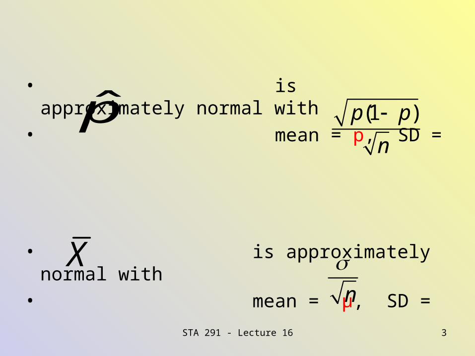
• is approximately normal with
• mean = p, SD =
• is approximately normal with
• mean = μ, SD =
STA 291 - Lecture 16 3
p̂
Xn
(1 )p p
n
STA 291 - Lecture 16 4
Central Limit Theorem
• For random sampling, as the sample size n grows, the sampling distribution of the sample mean approaches a normal distribution. So does the sample proportion
• Amazing: This is the case even if the population distribution is discrete or highly skewed
• The Central Limit Theorem can be proved mathematically
• We will verify it experimentally in the lab sessions
Xp̂
STA 291 - Lecture 16 5
Central Limit Theorem
• Online applet 1
http://www.stat.sc.edu/~west/javahtml/CLT.html
• Online applet 2
http://bcs.whfreeman.com/scc/content/cat_040/spt/CLT-SampleMean.html
STA 291 - Lecture 16 6
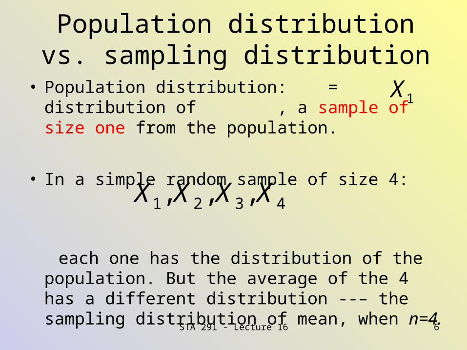
Population distribution vs. sampling distribution
• Population distribution: = distribution of , a sample of size one from the population.
• In a simple random sample of size 4:
each one has the distribution of the population. But the average of the 4 has a different distribution --– the sampling distribution of mean, when n=4.
1X
1 2 3 4, , ,X X X X
STA 291 - Lecture 16 7
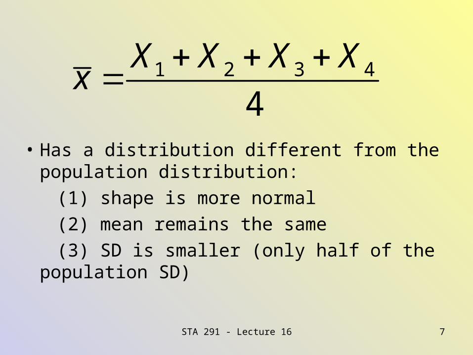
• Has a distribution different from the population distribution:
(1) shape is more normal
(2) mean remains the same
(3) SD is smaller (only half of the population SD)
1 2 3 4
4
X X X Xx
STA 291 - Lecture 16 8
Population Distribution
• Distribution from which we select the sample
• Unknown, we want to make inference about its parameters
• Mean = ?
• Standard Deviation = ?
STA 291 - Lecture 16 9
Sample Statistic
• From the sample X1, …, Xn we compute descriptive statistics
• Sample Mean =
• Sample Standard Deviation =
• Sample Proportion =
They all can be computed given a sample.
STA 291 - Lecture 16 10
Sampling Distribution of a sample statistic
• Probability distribution of a statistic (for example, the sample mean)
• Describes the pattern that would occur if we could repeatedly take random samples and calculate the statistic as often as we wanted
• Used to determine the probability that a statistic falls within a certain distance of the population parameter
• The mean of the sampling distribution of is =• The SD of is also called Standard Error =
XX
STA 291 - Lecture 16 11
• The 3 features for the sampling distribution of sample mean also apply to sample proportion. (1. approach normal, 2. centered at p; 3. less and less SD)
• This sampling distribution tells us how far or how close between “p” and
• One quantity we can compute, the other we want to know
p̂
STA 291 - Lecture 16 12
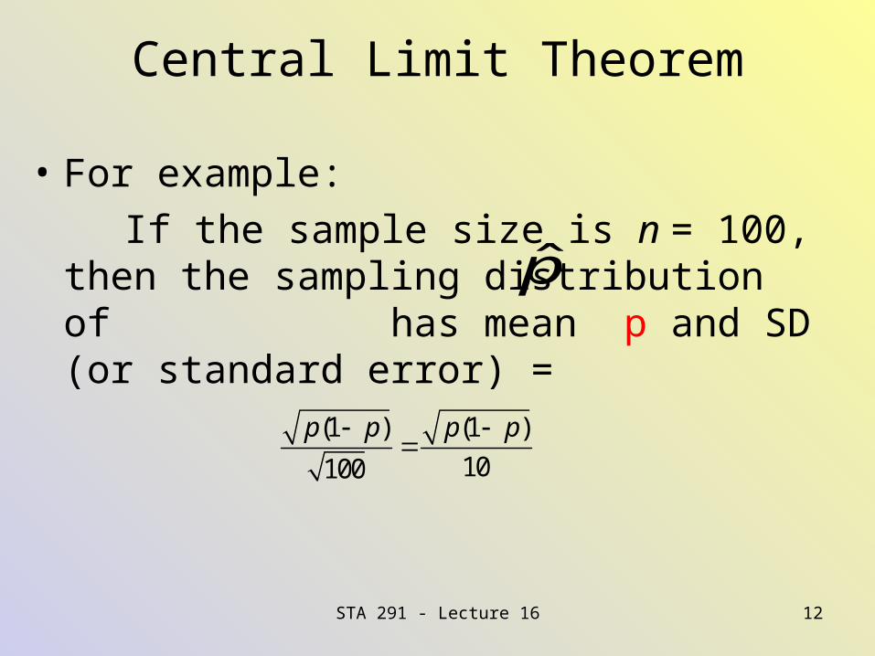
Central Limit Theorem
• For example:
If the sample size is n = 100, then the sampling distribution of has mean p and SD (or standard error) =
(1 ) (1 )
10100
p p p p
p̂
STA 291 - Lecture 16 13
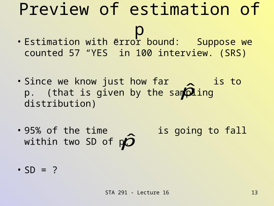
Preview of estimation of p• Estimation with error bound: Suppose we
counted 57 “YES” in 100 interview. (SRS)
• Since we know just how far is to p. (that is given by the sampling distribution)
• 95% of the time is going to fall within two SD of p.
• SD = ?
p̂
p̂
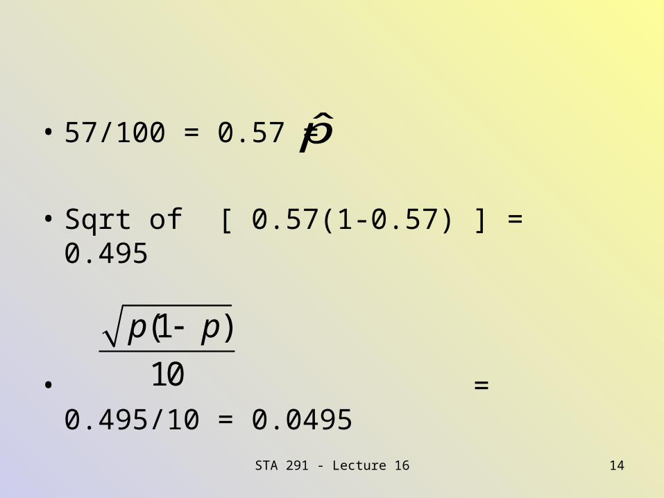
• 57/100 = 0.57 =
• Sqrt of [ 0.57(1-0.57) ] = 0.495
• = 0.495/10 = 0.0495
STA 291 - Lecture 16 14
p̂
(1 )
10
p p
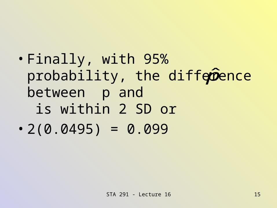
• Finally, with 95% probability, the difference between p and is within 2 SD or
• 2(0.0495) = 0.099
STA 291 - Lecture 16 15
p̂
STA 291 - Lecture 16 16
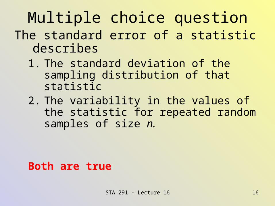
Multiple choice questionThe standard error of a statistic describes
1. The standard deviation of the sampling distribution of that statistic
2. The variability in the values of the statistic for repeated random samples of size n.
Both are true
STA 291 - Lecture 16 17
Multiple Choice QuestionThe Central Limit Theorem implies that
1. All variables have approximately bell-shaped sample distributions if a random sample contains at least 30 observations
2. Population distributions are normal whenever the population size is large
3. For large random samples, the sampling distribution of the sample mean (X-bar) is approximately normal, regardless of the shape of the population distribution
4. The sampling distribution looks more like the population distribution as the sample size increases
• In previous page, 3 is correct.
STA 291 - Lecture 16 18
STA 291 - Lecture 16 19
Chapter 10• Statistical Inference: Estimation of p
– Inferential statistical methods provide predictions about characteristics of a population, based on information in a sample from that population
– For quantitative variables, we usually estimate the population mean (for example, mean household income)
– For qualitative variables, we usually estimate population proportions (for example, proportion of people voting for candidate A)
STA 291 - Lecture 16 20
Two Types of Estimators• Point Estimate
– A single number that is the best guess for the parameter
– For example, the sample mean is usually a good guess for the population mean
• Interval Estimate (harder)
=point estimator with error bound– A range of numbers around the point estimate– To give an idea about the precision of the estimator – For example, “the proportion of people voting for A is
between 67% and 73%”
STA 291 - Lecture 16 21
Point Estimator• A point estimator of a parameter is a sample
statistic that predicts the value of that parameter
• A good estimator is – Unbiased: Centered around the true parameter – Consistent: Gets closer to the true parameter as
the sample size gets larger– Efficient: Has a standard error that is as small as
possible (made use of all available information)
STA 291 - Lecture 16 22
Efficiency• An estimator is efficient if its standard error
is small compared to other estimators• Such an estimator has high precision• A good estimator has small standard
error and small bias (or no bias at all)
• The following pictures represent different estimators with different bias and efficiency
• Assume that the true population parameter is the point (0,0) in the middle of the picture
STA 291 - Lecture 16 23
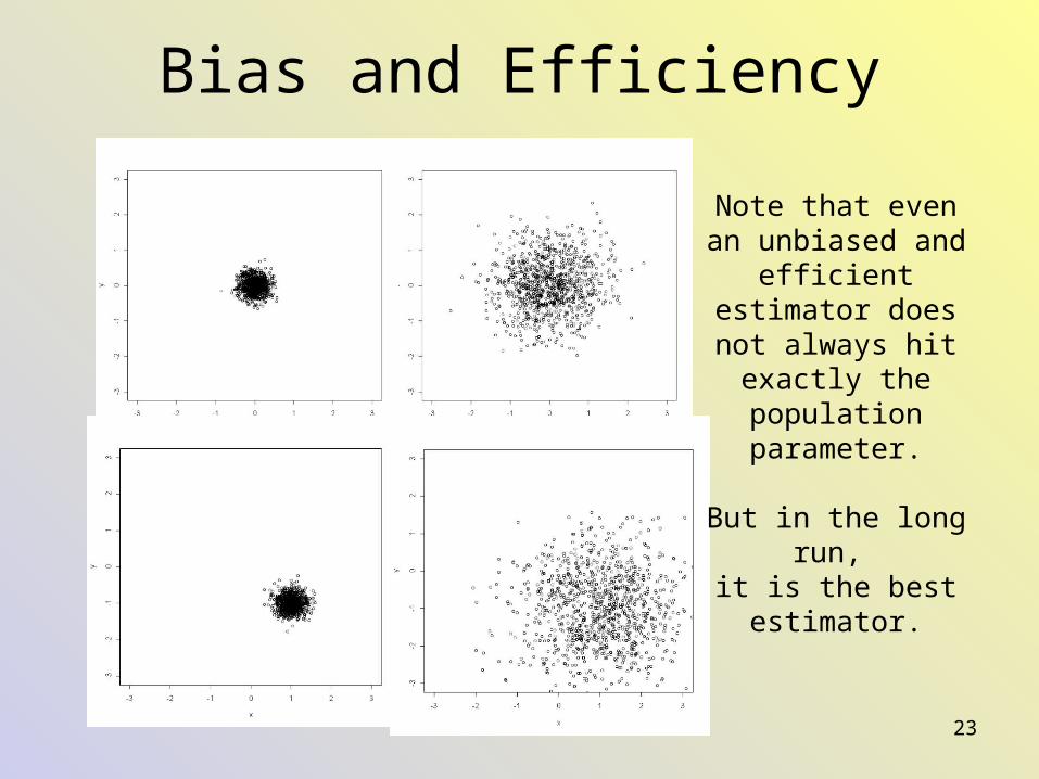
Bias and Efficiency
Note that even an unbiased and
efficient estimator does not always hit
exactly the population parameter.
But in the long run, it is the best estimator.
• Sample proportion is an unbiased estimator of the population proportion.
• It is consistent and efficient.
STA 291 - Lecture 16 24
STA 291 - Lecture 16 25
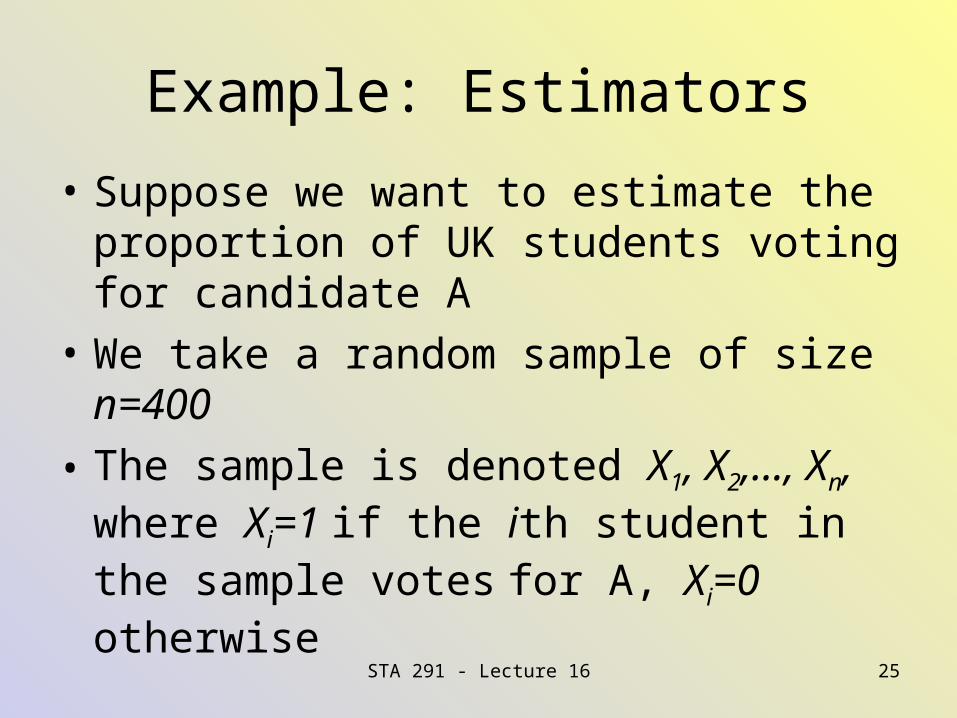
Example: Estimators
• Suppose we want to estimate the proportion of UK students voting for candidate A
• We take a random sample of size n=400
• The sample is denoted X1, X2,…, Xn, where Xi=1 if the ith student in the sample votes for A, Xi=0 otherwise
STA 291 - Lecture 16 26
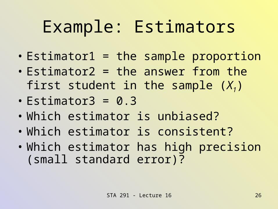
Example: Estimators
• Estimator1 = the sample proportion• Estimator2 = the answer from the first
student in the sample (X1)• Estimator3 = 0.3• Which estimator is unbiased?• Which estimator is consistent? • Which estimator has high precision (small
standard error)?
STA 291 - Lecture 16 27
Attendance Survey Question
• On a 4”x6” index card– Please write down your name and
section number
– Today’s Question:
– Table or web page for Normal distribution? Which one you like better?
STA 291 - Lecture 16 28
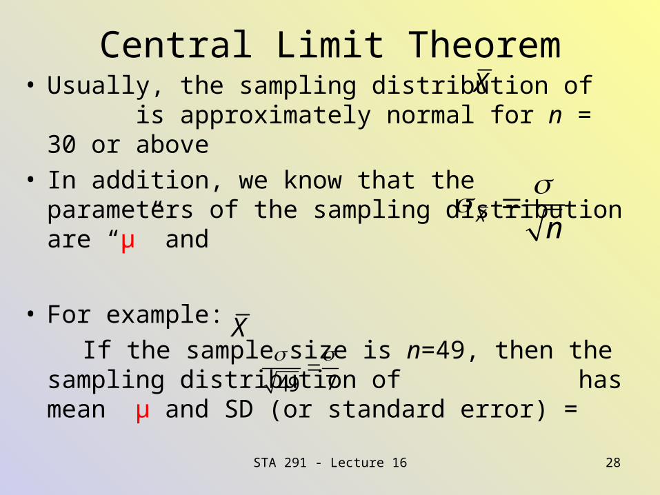
Central Limit Theorem• Usually, the sampling distribution of is
approximately normal for n = 30 or above• In addition, we know that the parameters of the
sampling distribution are “μ” and
• For example:
If the sample size is n=49, then the sampling distribution of has mean μ and SD (or standard error) =
X
X n
749
X
STA 291 - Lecture 16 29
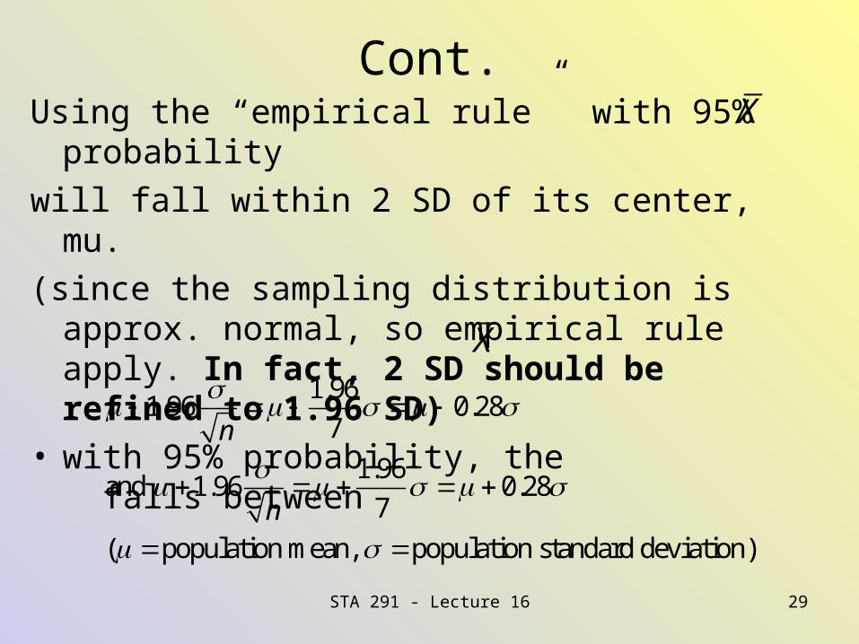
Cont.Using the “empirical rule” with 95% probability
will fall within 2 SD of its center, mu.
(since the sampling distribution is approx. normal, so empirical rule apply. In fact, 2 SD should be refined to 1.96 SD)
• with 95% probability, the falls between
X
1.961.96 0.28
7
1.96and 1.96 0.28
7
( population mean, population standard deviation)
n
n
X
STA 291 - Lecture 16 30
Unbiased
• An estimator is unbiased if its sampling distribution is centered around the true parameter
• For example, we know that the mean of the sampling distribution of “X-bar” equals “mu”, which is the true population mean
• So, “X-bar” is an unbiased estimator of “mu”
STA 291 - Lecture 16 31
Unbiased• However, for any particular sample, the sample
mean “X-bar” may be smaller or greater than the population mean
• “Unbiased” means that there is no systematic under- or overestimation
STA 291 - Lecture 16 32
Biased
• A biased estimator systematically under- or overestimates the population parameter
• In the definition of sample variance and sample standard deviation uses n-1 instead of n, because this makes the estimator unbiased
• With n in the denominator, it would systematically underestimate the variance
STA 291 - Lecture 16 33
Point Estimators of the Mean and Standard Deviation
• The sample mean is unbiased, consistent, and (often) relatively efficient for estimating “mu”
• The sample standard deviation is almost unbiased for estimating population SD (no easy unbiased estimator exist)
• Both are consistent