Electronic copy available at: http://ssrn.com/abstract=1134660

1

The optimal covenant threshold in loan contracts

Flavio Bazzana Department of Economics and Management

Via Inama, 5 University of Trento

I–38122 Trento ITALY flavio.bazzana@unitn.it

ph. +39 0461 283107 fax +39 0461 282124

Abstract Despite the growing importance of covenants and the increasing frequency with which covenants are included in debt contracts, the role of covenant strength in bank loans has not received much attention in the theoretical literature to date. The goal of our paper is to provide a theoretical model within a standard credit risk framework that can be used to compute the optimal covenant strength for bank loans. In our model, a risk-neutral bank finances a firm that invests in a two-period, two-state project. We find that the expected loss rate (and, accordingly, the interest rate) decreases if a covenant is used in the contract. In the most general formulation of our model, which is composed of a loan with a covenant on the total assets of the firm and asymmetric information, we find that the expected loss rate depends on two sources of risk: (i) investment project risk and (ii) the risk from the entrepreneur’s behaviour. In this case, the expected loss rate for the financed quote values is minimal for a given covenant strength. JEL classification codes: G21, G28 Keywords: covenants, crediti risk, loans pricing

1. Introduction

Despite the growing importance of covenants and the increasing rate with which cove-nants are included in debt contracts (Billett, Dolly King, and Mauer 2007; Nini, Smith, and Sufi 2009; Kwan and Carleton 2010), the role of covenant strength in bank loans has not received substantial attention in the theoretical literature to date. Many empir-ical papers have investigated the relationship between covenant strength and the addi-tional variables used to calculate expected loss rates (Asquith, Beatty, and Weber 2005; Paglia and Mullineaux 2006; Ackert, Huang, and Ramirez 2007; Sufi 2009; Demiroglu and James 2010; Godlewski and Weill 2011), but only a recent paper by Gârleanu and Zwiebel (2009) and a working paper by Bazzana and Broccardo (2012) provide a theo-

Electronic copy available at: http://ssrn.com/abstract=1134660

2

retical model that explains covenant strength. Gârleanu and Zwiebel (2009) propose a general model that analyses covenant strength in debt contracts using a property rights approach. Bazzana and Broccardo (2012) analyse the differences in optimal covenant strength between public and private debt. The goal of our paper is to provide a theo-retical model with which to calculate the optimal covenant strength that minimises ex-pected loss rates (elr) for bank loans.

The following variables are standard for calculating elr in the credit risk literature (Duffie and Singleton, 2003; Lando, 2004) and the Basel II framework (Basel Commit-tee on Banking Supervision, 2005): (i) the probability of default (PD), (ii) the loss giv-en default (LGD), and (iii) the exposure at default (EAD).

In estimating the PD, banks (which primarily conduct the monitoring) analyse data from their daily transactions with the firm in question. Variation in the PD could shift the firm to a different rating class, which would render the initial spread inadequate. The bank would then have to bear a greater expected loss than initially estimated. Short-term operations provide the bank with considerable flexibility because the bank may ask for a withdrawal or easily adapt the spread. In contrast, for long-term opera-tions, the bank cannot contractually request an anticipated refund; therefore, when the rating class changes, the bank cannot effectively change the spread or ask for such a refund. Thus, in long-term operations, the bank may include covenants in the contract that are calculated in accordance with the financial ratios used to estimate the PD. Under such covenants, the bank can request repayment of outstanding debt if the cov-enant has been violated (i.e., if the rating class of the firm changes). As noted by Rajan and Winton (1995), the inclusion of covenants in long-term operations increases the flexibility of bank decisions and enables banks to use information more efficiently, which facilitates more effective monitoring (Nini, Smith, and Sufi 2009).

For LGD monitoring, two factors are significant: the company’s level of liquidity and the seniority of the loan. In a crisis situation, assets could lower the degree of li-quidity and affect the LGD. In such a case, the inclusion of covenants in the contract that bind the company to render certain corporate assets available and reduce the LGD enables the bank to demand the repayment of outstanding debt. Covenants are also extremely important for safeguarding loan seniority because they reduce LGD estimat-ed values (J Niskanen and M Niskanen 2004; Paglia and Mullineaux 2006; Moir and Sudarsanam 2007). As with the PD, covenants also facilitate monitoring the position; thus, an operation can be avoided in which the elr is unrelated to the initial spread.

Finally, the EAD may be affected by covenants that provide the bank with prior knowledge of the firm’s risk. For example, by including covenants that address risky events, such as loan rate non-payment or shareholder structure modification, the bank can reduce exposure to firms that are more likely to default. This protection can reduce the initial EAD estimation.

Despite the theoretical importance of covenants for elr estimation, the Basel II

3

framework does not dwell on this issue and acknowledges its importance only through EAD evaluations. Only the banks that adopt the advanced internal rating-based ap-proach (IRBA) can calculate the capital requirements for an operation and consider the effectiveness of covenants in their EAD evaluations. Under the other two approaches, the standard and IRBA foundation approaches, the supervisory institution assigns EAD values to different types of operations. Even standard credit risk models do not directly account for the role of covenants (for a review, see Duffie and Singleton, 2003; Lando, 2004). In addition, the principal rating agencies do not formally consider the importance of covenants in the rating criteria (see May and Verde, 2006, for Fitch Rat-ings; Standard and Poor’s, 2006; Padgett, 2006, for Moody’s).

Herein, we propose a loan covenant model within a standard credit risk framework in which the covenant strength is calculated by minimising the expected loss rate. This model is based on Black and Cox (1976), but it replaces the continuous time methodol-ogy used in the study with a discrete time and state of nature approach. Loan covenant pricing follows the Credit Metrics model (Gupton, Finger and Bhatia, 1997) by assum-ing that the bank is risk-neutral. We focus on covenant strength, as in Gârleanu and Zwiebel (2009) and Bazzana and Broccardo (2012). Unlike Gârleanu and Zwiebel (2009), we assume that the firm can avoid a covenant violation by increasing its capi-tal. We also assume that the firm’s behaviour depends on covenant strength. Different from Bazzana and Broccardo (2012), we use a two-stage method and a more standard approach to compute the loan’s expected loss rate. We find that the elr has a minimum value for a given financial covenant strength, and this optimal point can be calculated using a minimisation procedure. The model introduces an innovative process and unique results to the existing literature: (i) the model analyses how firms behave to avoid violating the covenant, and (ii) it facilitates the identification of optimal cove-nant strength for the bank. To our knowledge, this is the only paper that has presented such results.

The paper proceeds as follows. First, we present loan pricing for symmetric infor-mation and highlight the difference between a standard loan and a loan with a cove-nant. We then modify the model by introducing asymmetric information between the bank and firm and present the results from the optimisation procedure. The conclusions follow.

2. The model with symmetric information

We consider an entrepreneur investing in a two-year project with an initial cost nor-malised to 1. The value of the project follows a binomial stochastic process with drift µ and standard deviation σ. A graphical representation of the investment project is shown in Fig. 1, wherein u indicates up, d indicates down and p is the probability of a decrease in each node. The variables are functions of the drift and standard deviation

4

(i.e., u = u σ( ) ,

d = d σ( ) , and

p = p µ,σ( ) , as is typical)1.

u

d

u 2

ud

d 2

1 − p

p

p

1 − p

1

p

1 − p

t = 0 t = 1 t = 2

Figure 1. Graphical representation of the investment project value for the two

periods with the corresponding probabilities.

The project is financed through a bank loan, α < 1 at a gross rate r > 1 , with in-

terest paid, a capital refund αr 2 at maturity, and equity for the remaining portion. The bank receives the investment project as collateral, and the entrepreneur will sell the investment at the end of the second year to repay the loan. Both the bank and en-trepreneur understand the stochastic process followed by the investment project, and the only risk is from the probability p; thus, we have symmetric information. To simpli-fy the approach, we assume a single default position in period two, i.e.,

d2 < αr 2 < ud , (1)

and the binomial process has the property ud ≡ 1 .

2.1. The standard loan

Under the above hypothesis, the bank will have a default scenario only in period two

for a standard loan when the value of the investment project is d2 . Fig. 2 provides a graphical representation of the cash flow for the bank given the possible values for the investment project.

1 In the binomial model, p is typically defined as the probability of an increase. We are interested in the

probability of a decrease, which is the risk associated with lending; thus, we reverse the meaning of the notation.

5

αr 2

d 2

1 − p 2

p 2

t = 0 t = 2

−α

Figure 2. A graphical representation of the cash flow for the bank with the cor-

responding probability and a standard loan. Given these assumptions, the expected loss rate for the bank is

elr = PD×LGD = PD×

EAD −READ

⎛

⎝⎜⎜⎜

⎞

⎠⎟⎟⎟⎟ , (2)

where PD is the probability that the firm will default and LGD is the loss given default (i.e., the ratio between the loss upon default and exposure at default (EAD)). R is the

value of recovery upon default. In the model, PD = p2 and LGD = αr 2 −d2( ) αr 2 ;

thus, the elr becomes

elr = p2 1−

d2

αr 2

⎛

⎝⎜⎜⎜⎜

⎞

⎠⎟⎟⎟⎟⎟. (3)

Assuming risk neutrality, the bank will choose an interest rate equal to the expected refund of the loan with the loan amount determined by the gross risk-free rate i:

p2d2 + 1− p2( )αr 2 = αi2 . (4)

Resolving equation (4) with respect to the interest rate, we obtain the following:

r 2 =αi2 − p2d2

α 1− p2( )=αi2 −PD×Rα 1−PD( )

. (5)

Furthermore, from equation (3), the elr value can be written as

elr = p2 αi

2 −d2

αi2 − p2d2. (6)

Defining the model variables of set S as

S ≡ d,p,i,α( ) 0 < d < 1; 0 < p < 1; i > 1; 0 < α < 1{ } , (7)

6

the overall feasible set for the standard loan (i.e., the intersection between the default condition (1) and set S) can be rewritten as follows:

Sr ≡ d,p,i,α( ) d2

i2< α <

1− p2 1−d2( )i2

; d,p,i,α( ) ∈ S⎧⎨⎪⎪⎪

⎩⎪⎪⎪

⎫⎬⎪⎪⎪

⎭⎪⎪⎪

. (8)

Under these assumptions, the bank experiences the following two types of complica-tions: (i) limited decision-making flexibility and (ii) a high level of risk. The bank has limited flexibility because the elr can only be modified by changing the financed quote. For example, if the entrepreneur will not accept a reduction in the portion financed and the bank has an operational limit on the elr for new operations, the operation cannot be completed. More important is the level of risk during the life of the loan. In the first period, if the value of the investment project is d, the elr will increase because the PD increases to the p value, and the R remains the same. The bank cannot increase the interest rate to accommodate the new level of risk because it was fixed at the beginning of the contract, but the bank cannot sell the collateral because the firm is not in de-fault (the only payment to the bank is in period two). A covenant can provide a possi-ble solution to both problems.

2.2. The loan with a restrictive covenant on the investment project

Suppose that the bank introduces the following restrictive covenant into the loan con-tract: “If the value of the investment project in period one is less than d, the bank can sell the collateral to refund the loan early”. The value of the loan for early repayment

is αrcp , where the subscript cp indicates the covenant on the investment project. To

eliminate trivial cases, we assume that the bank has no incentive to request the antici-pated refund of the loan (i.e., the capitalised value of the collateral must be lower than the value of the loan at maturity)2:

di < αrcp

2 . (9)

If the value of the investment project is d (i.e., the firm will be in technical default), the bank can sell the collateral to refund the loan early, or it can waive the covenant violation. A risk-neutral bank will sell the collateral if the anticipated refund capitalised at risk-free rate i is greater than the expected value of the loan refund in period two, as follows3:

2 This condition contains the non-trivial condition (1) for the standard loan. 3 Otherwise, if the bank waives the covenant violation, the elr and corresponding interest rate r are equal

to those values in the standard case.

7

di > pd2 + 1− p( )αrcp2 . (10)

A graphical representation of the cash flow for the bank given the possible values of the investment project is depicted in Fig. 3.

di

1 − p

p

- α

t = 0 t = 2

αrcp2

Figure 3. A graphical representation of the cash flow for the bank with the cor-

responding probability for a loan with a restrictive covenant and anticipated refund of the loan invested at risk-free rate i.

The only default position is in period one, when the bank sells the collateral for a

loss; thus, PD = p . The recovery is the capitalised anticipated refund at the risk-free

rate i (i.e., R = di ). Given these assumptions, the elr is as follows:

elrcp = p 1−di

αrcp2

⎛

⎝

⎜⎜⎜⎜⎜

⎞

⎠

⎟⎟⎟⎟⎟⎟. (11)

As in the standard model, the bank chooses an interest rate equal to the expected refund of the loan when the amount of the loan is determined at the gross risk-free rate i:

pdi + 1− p( )αrcp2 = αi2 . (12)

Resolving equation (12) for the interest rate, we obtain

rcp

2 =αi2 − pdiα 1− p( )

; (13)

using equation (13) in equation (11), we obtain

elrcp = p

αi −dαi − pd

. (14)

As above, we can define the overall feasible set of the loan with a covenant on the investment project (i.e., the intersection between inequality (9) and inequality (10) us-

8

ing expression (13)) and set S as follows:

Scp ≡ d,p,i,α( ) d

i< α <

d

i2i −dp + pi( ); d,p,i,α( ) ∈ S

⎧⎨⎪⎪⎩⎪⎪

⎫⎬⎪⎪⎭⎪⎪. (15)

Rearranging the difference between the interest rate on the standard loan (5) and the loan with a covenant (13), we can compare the two interest rates as follows:

r 2 − rcp2 =

pd

i2i −dp + pi( )− α

⎛

⎝⎜⎜⎜

⎞

⎠⎟⎟⎟⎟

1− p2( )α. (16)

For a correct comparison, we must define expression (16) at the intersection be-

tween the two feasible sets (i.e., Sr ∩ Scp ≡ Sr∩cp ):

Sr∩cp = Scp . (17)

Thus, expression (16) becomes the following:

r 2 − rcp

2( )d,p,i,α( )∈Sr∩cp

> 0 , (18)

which is consistent with empirical observations on the impact of covenants on loan con-tract interest rates. Using the same method,

elr −elrcp( )

d,p,i,α( )∈Sr∩cp

> 0 . (19)

The bank can increase its flexibility using this loan contract design and offering a lower interest rate to the firm, but the entrepreneur cannot avoid the possibility of vio-lating the covenant (i.e., technical default) in period one. If the latter occurs, the en-trepreneur will lose all of its initial equity because the bank will sell the collateral. However, with the opportunity to avoid technical default, the entrepreneur can achieve a positive outcome after refunding the loan if the value of the investment project in period two is 1. For the entrepreneur to meet the covenant, the bank can define the covenant based on the total assets of the firm instead of the value of the investment project.

2.3. The loan with a restrictive covenant on total assets

Suppose now that the bank composes the restrictive covenant in the loan contract as follows: “If the value of the total assets of the firm is lower than a fixed threshold q, the bank can sell the collateral to refund the loan early”. Because the total assets of the firm in period zero are equal to the investment project with its value normalised to 1, the possible range for q is between d and 1 (or d ≤ q ≤ 1). The strength s of the cove-

9

nant ( 0 ≤ s ≤ 1) is the relative distance between q and d, as follows:

s =

q −d1−d

. (20)

Thus, the covenant is stronger for higher values. In period one, if the value of the in-vestment project is d, the firm has a negative net income. If the value of the asset de-creases from 1 to d, the value of the debt remains constant at α because the loan will be refunded only upon its maturity. Consequently, the value of the equity will decrease

from 1− α to d − α (i.e., 1− α− 1−d( ) ). According to this hypothesis, if the value

of the investment project at period one is d, the covenant is violated, and the firm is in technical default. However, the entrepreneur can meet the covenant with an equity in-

crease, q −d = s 1−d( ) , and by investing the money at gross risk-free rate i.

The entrepreneur must consider the two different alternatives: (i) do not increase the capital with a loss of initial capital, 1− α , or (ii) meet the covenant with possible revenue in period two if the value of the investment project is 1. As an example, a risk-neutral entrepreneur will prefer the second alternative only if the discounted expected revenue in period two is greater than the capital increase, i.e.,

1− p( ) 1− αrca2( )

i> s 1−d( ) , (21)

where the subscript ca indicates a covenant on the total assets. From the bank’s per-spective and assuming that the entrepreneur respects the covenant upon its violation, if

the value of the investment project in period two is d2 , the bank receives

d2 + s 1−d( )i . To eliminate trivial cases, we assume that even with the equity in-

crease, the bank loses the following:

d2 + s 1−d( )i < αrca,r

2 , (22)

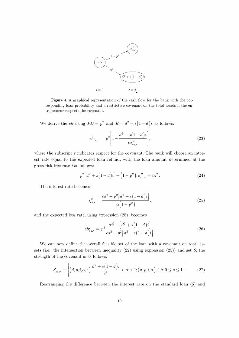
where the subscript r indicates respect for the covenant. Fig. 4 shows a graphical repre-sentation of the cash flow for the bank if the entrepreneur increases the capital given the possible value of the investment project.

10

1 − p 2

p 2

t = 0 t = 2

αrca,r2

d2 + s 1−d( )i

−α

Figure 4. A graphical representation of the cash flow for the bank with the cor-

responding loan probability and a restrictive covenant on the total assets if the en-trepreneur respects the covenant.

We derive the elr using PD = p2 and R = d2 + s 1−d( )i as follows:

elrca,r = p2 1−d2 + s 1−d( )i

αrca,r2

⎡

⎣

⎢⎢⎢

⎤

⎦

⎥⎥⎥, (23)

where the subscript r indicates respect for the covenant. The bank will choose an inter-est rate equal to the expected loan refund, with the loan amount determined at the gross risk-free rate i as follows:

p2 d2 + s 1−d( )i⎡⎣⎢

⎤⎦⎥ + 1− p2( )αrca,r

2 = αi2 . (24)

The interest rate becomes

rca,r2 =

αi2 − p2 d2 + s 1−d( )i⎡⎣⎢

⎤⎦⎥

α 1− p2( ), (25)

and the expected loss rate, using expression (25), becomes

elrca,r = p2αi2 − d2 + s 1−d( )i⎡

⎣⎢⎤⎦⎥

αi2 − p2 d2 + s 1−d( )i⎡⎣⎢

⎤⎦⎥. (26)

We can now define the overall feasible set of the loan with a covenant on total as-sets (i.e., the intersection between inequality (22) using expression (25)) and set S; the strength of the covenant is as follows:

Sca,r ≡ d,p,i,α,s( )d2 + s 1−d( )i

i2< α < 1; d,p,i,α( ) ∈ S;0 ≤ s ≤ 1

⎧⎨⎪⎪⎪

⎩⎪⎪⎪

⎫⎬⎪⎪⎪

⎭⎪⎪⎪. (27)

Rearranging the difference between the interest rate on the standard loan (5) and

11

the loan with a covenant on the total assets (25), we obtain the following:

r 2 − rca,r2 =

p2 1−d( )is1− p2( )α

, (28)

which is always greater than zero for each model variable value in set S. This is also true at the intersection between the two feasible sets, as follows:

Sr∩ca,r = d,p,i,α,s( ) d2

i2< α <

1− p2 1−d2( )i2

; d,p,i,α( ) ∈ S;0 ≤ s ≤ 1⎧⎨⎪⎪⎪

⎩⎪⎪⎪

⎫⎬⎪⎪⎪

⎭⎪⎪⎪; (29)

thus, expression (28) becomes

r 2 − rca,r

2( )d,p,i,α,s( )∈Sr∩ca ,r

> 0 , (30)

which is also consistent with empirical observations on the impact of covenants on the interest rates of loan contracts.

However, if an entrepreneur will not increase the capital upon violating the cove-nant, a bank will sell the collateral in period one. This the same outcome as for a loan with a covenant on an investment project ( PD = p and R = di ). The expected loss

rate becomes

elrca,v = p 1−di

αrca,v2

⎛

⎝

⎜⎜⎜⎜⎜

⎞

⎠

⎟⎟⎟⎟⎟⎟, (31)

where the subscript v indicates a covenant violation. The interest rate becomes

rca,v

2 =αi2 − pdiα 1− p( )

= rcp2 , (32)

and the direct elr is as follows:

elrca,v = p

αi −dαi − pd

= elrcp . (33)

The feasible set is the same for a covenant on an investment project (i.e.,

Sca,v = Scp ) and the intersection of the two feasible sets (i.e.,

Sr∩ca,v = Scp ). Thus, from

inequality (18), we obtain

r 2 − rca,v

2( )d,p,i,α( )∈Sr∩ca ,v

≥ 0 . (34)

This result is consistent with empirical observations.

12

3. The model with asymmetric information

We now introduce asymmetric information into the latter case (i.e., the loan with a restrictive covenant on the total assets of the firm). We assume that at period zero, the bank does not know the behaviour of the entrepreneur at period one if the value of the investment project is d (i.e., if the firm is in technical default). We implicitly assume that the entrepreneur will increase the capital upon a covenant violation not only for risk-neutral expected equity cash flow, as in the previous case, but also for additional variables not directly observable by the bank. These variables can include, for example, bankruptcy costs, reputational costs and limited funds at the entrepreneur’s disposal. However, it is realistic to assume that the bank knows the past behaviour of entrepre-neurs with regard to covenant strength. If the covenant is relaxed (i.e., a lower s), a large number of entrepreneurs will decide on a capital increase because it has low value. With a tighter covenant (i.e., a higher s), a large number of entrepreneurs will likely place the firm in technical default and violate the covenant. Thus, we assume that the

bank knows the cumulative density function F s( ) , which is the probability that the

entrepreneur will not increase the capital if the covenant strength is s. In this case, the firm is in technical default because the covenant has been violated

and the entrepreneur did not increase the capital. The bank has two possibilities: (i) sell the collateral or (ii) waive the covenant violation. The bank, as in equation (10), will sell the collateral only if the money generated, capitalised at risk-free rate i, is greater than the expected value of the loan refund in period two, i.e.,

di > pd2 + 1− p( )αrca,s

2 , (35)

in which s indicates selling the collateral. Fig. 5 shows a graphical representation of the loan values for the bank in this case.

13

p

t = 0 t = 1 t = 2

1 − p

di

1 − p

1 − F(s)

F(s)

d2 + s 1−d( )ip

−α

αrca,s2

Figure 5. A graphical representation of the loan values for the bank and the cor-

responding probability with asymmetric information with a covenant on total as-sets. The bank will sell the collateral if the entrepreneur does not increase the capi-tal to avoid a covenant violation.

To eliminate trivial cases, we assume that even with an equity increase, the bank in-

curs a loss, i.e.,

d2 + s 1−d( )i < αrca,s

2 . (36)

In accordance with these hypotheses, the expected loss rate for the bank is calculat-ed as a weighted average elr of the loan upon violation and respect, as follows:

elrca,s = F s( )×elrca,v + 1−F s( )⎡

⎣⎤⎦elrca,r , (37)

where F 0,1{ }( ) = 0,1{ } . Using expressions (23) and (31) and defining a unique inter-

est rate, we generate the following:

elrca,s = F s( )p 1−di

αrca,s2

⎛

⎝

⎜⎜⎜⎜⎜

⎞

⎠

⎟⎟⎟⎟⎟⎟+ 1−F s( )⎡⎣

⎤⎦ p

2 1−d2 + s 1−d( )i

αrca,s2

⎡

⎣

⎢⎢⎢

⎤

⎦

⎥⎥⎥. (38)

The bank will choose an interest rate equal to the expected refund of the loan with the amount of the loan determined at the gross risk-free rate i. To determine the loan interest rate, we must solve the following equation:

p F s( )di + 1−F s( )( ) p d2 + s 1−d( )i( ) + 1− p( )αrca,s

2⎡⎣⎢

⎤⎦⎥{ } + 1− p( )αrca,s

2 = αi2 , (39)

which becomes

14

rca,s

2 =αi2 − p F s( )di + 1−F s( )( )p d2 + s 1−d( )i( )⎡

⎣⎢⎤⎦⎥

α 1− p F s( ) + 1−F s( )( )p( )⎡⎣

⎤⎦

. (40)

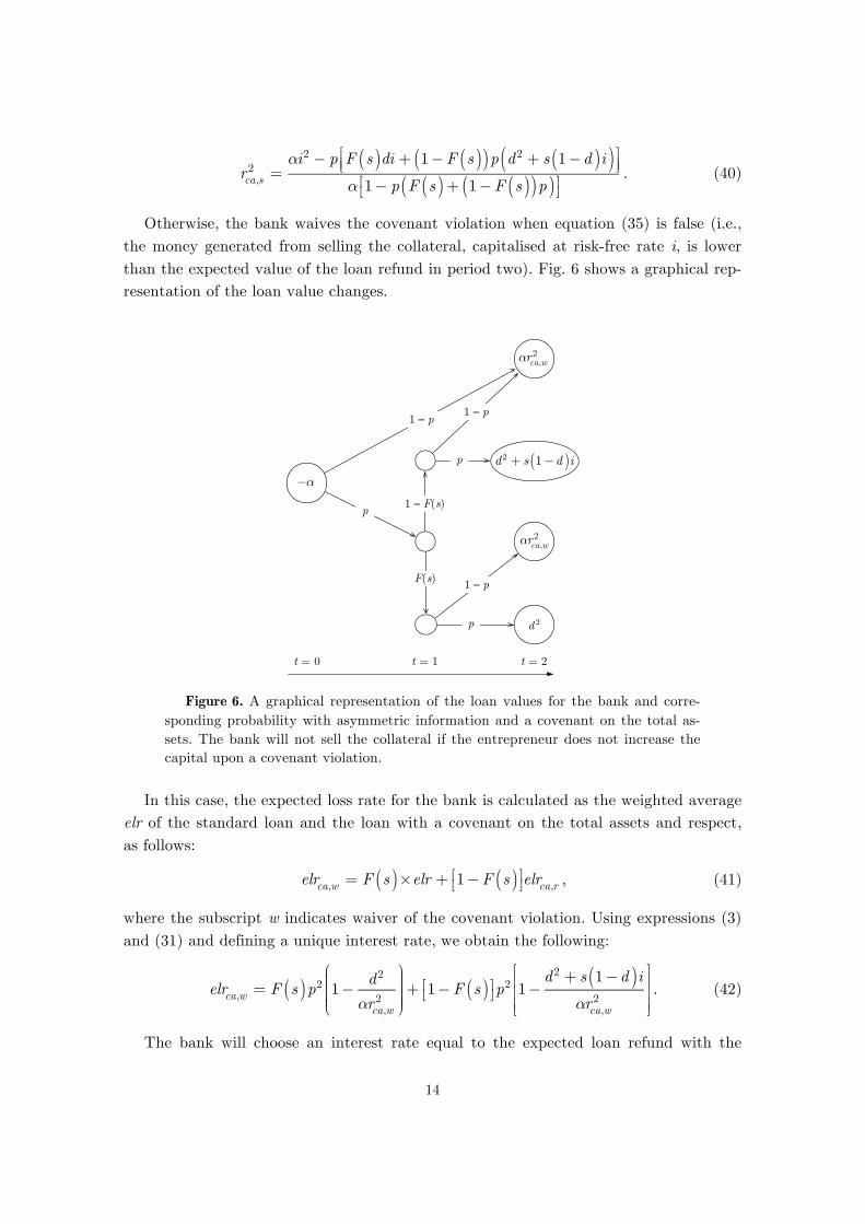
Otherwise, the bank waives the covenant violation when equation (35) is false (i.e., the money generated from selling the collateral, capitalised at risk-free rate i, is lower than the expected value of the loan refund in period two). Fig. 6 shows a graphical rep-resentation of the loan value changes.

p

t = 0 t = 1 t = 2

1 − p1 − p

1 − F(s)

F(s)

d2 + s 1−d( )ip

−α

p d 2

1 − p

αrca,w2

αrca,w2

Figure 6. A graphical representation of the loan values for the bank and corre-

sponding probability with asymmetric information and a covenant on the total as-sets. The bank will not sell the collateral if the entrepreneur does not increase the capital upon a covenant violation.

In this case, the expected loss rate for the bank is calculated as the weighted average

elr of the standard loan and the loan with a covenant on the total assets and respect, as follows:

elrca,w = F s( )×elr + 1−F s( )⎡

⎣⎤⎦elrca,r , (41)

where the subscript w indicates waiver of the covenant violation. Using expressions (3) and (31) and defining a unique interest rate, we obtain the following:

elrca,w = F s( )p2 1−d2

αrca,w2

⎛

⎝

⎜⎜⎜⎜⎜

⎞

⎠

⎟⎟⎟⎟⎟⎟+ 1−F s( )⎡⎣

⎤⎦ p

2 1−d2 + s 1−d( )iαrca,w

2

⎡

⎣

⎢⎢⎢

⎤

⎦

⎥⎥⎥. (42)

The bank will choose an interest rate equal to the expected loan refund with the

15

loan amount determined at the gross risk-free rate i. To determine the loan interest rate, we must solve the following equation:

p F s( ) pd2 + 1− p( )αrca,w2⎡

⎣⎢⎤⎦⎥ +{

+ 1−F s( )( ) p d2 + s 1−d( )i( ) + 1− p( )αrca,w2⎡

⎣⎢⎤⎦⎥} + 1− p( )αrca,w

2 = αi2, (43)

which becomes

rca,w2 =

αi2 − p F s( )pd2 + 1−F s( )( )p d2 + s 1−d( )i( )⎡⎣⎢

⎤⎦⎥

α 1− p F s( )p + 1−F(s)( )p⎡⎣

⎤⎦{ }

=

=αi2 − p F s( )pd2 + 1−F s( )( )p d2 + s 1−d( )i( )⎡

⎣⎢⎤⎦⎥

α 1− p2( )

. (44)

3.1. Comparison and optimisation

We can now draw a comparison between the two expected loss rates4 from the model with asymmetric information, and the elr for the standard loan and the loan with a covenant on the investment project. First, under the hypothesis for the cumulative density function, the following holds:

elr = elrca,w s=0= elrca,s s=0

= elrca,w s=1

elrcp = elrca,s s=1

. (45)

Second, we must assign a value to the remaining variables in the model (i.e., from the investment project (p and d), gross risk-free rate i, and financed quote α ). Third,

we must analytically define the cumulative density function F s( ) . The simplest func-

tion for our limited interval 0,1⎡⎣⎤⎦ is triangular5, which is defined as follows:

F s,c( ) =

s2

c with 0 ≤ s ≤ c

1−1− s( )2

1−c with c ≤ s ≤ 1

⎧

⎨

⎪⎪⎪⎪⎪

⎩

⎪⎪⎪⎪⎪

, (46)

where c is the parameter shape ( 0 ≤ c ≤ 1). When c is lower, the probability is greater

4 Similar results, both qualitative and quantitative, can be obtained analysing the interest rates of the

model. There is a direct connection between elr and the corresponding interest rate; thus, to simplify the analysis, we only use the elr. 5 Another possible cumulative density function defined over a limited interval is the Beta function. We

obtain results similar to those from the triangular cumulative density.

16

that an entrepreneur will not increase the capital at a given s. However, when c is higher, it is more likely that an entrepreneur will not violate the covenant through a capital increase. Thus, formally, the following inequality is true:

∂F s,c( )∂c

≤ 0 . (47)

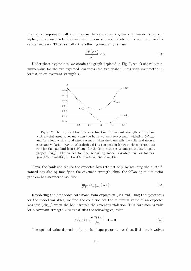
Under these hypotheses, we obtain the graph depicted in Fig. 7, which shows a min-imum value for the two expected loss rates (the two dashed lines) with asymmetric in-formation on covenant strength s.

0.2 0.4 0.6 0.8 1.0s

0.010

0.015

0.020

0.025

0.030

0.035

0.040

elr

elrca,w

elrca,s

elrcp

elr

Figure 7. The expected loss rate as a function of covenant strength s for a loan

with a total asset covenant when the bank waives the covenant violation (elrca,w) and for a loan with a total asset covenant when the bank sells the collateral upon a covenant violation (elrca,s). Also depicted is a comparison between the expected loss rate for the standard loan (elr) and for the loan with a covenant on the investment project (elrcp). The values for the remaining model variables are as follows:

p = 30% , d = 60% , i−1 = 4% , c = 0.85 , and α = 60% .

Thus, the bank can reduce the expected loss rate not only by reducing the quote fi-nanced but also by modifying the covenant strength; thus, the following minimisation problem has an internal solution:

mins∈ 0,1⎡⎣⎢

⎤⎦⎥elrca, s,w⎡⎣⎢

⎤⎦⎥

s,α( ) . (48)

Reordering the first-order conditions from expression (48) and using the hypothesis for the model variables, we find the condition for the minimum value of an expected loss rate (elrca,w) when the bank waives the covenant violation. This condition is valid for a covenant strength s that satisfies the following equation:

F s,c( ) + s

∂F s,c( )∂s

−1 = 0 . (49)

The optimal value depends only on the shape parameter c; thus, if the bank waives

17

the covenant violation, the optimal strength only depends on the expected behaviour of the entrepreneur. The other source of risk in the model, the investment project, does not play a role in determining s . If the bank sells the collateral upon a covenant viola-tion, the optimal covenant strength must satisfy the following equation:

1−d( )ip 1−F s,c( )⎡⎣

⎤⎦ 1 + p 1−F s,c( )( )⎡⎣

⎤⎦ +

+ di 1 + p + ps( )− i ps + iα( )−d2p⎡⎣⎢

⎤⎦⎥∂F s,c( )∂s

= 0. (50)

In this case, the optimal value of the covenant strength depends on the two sources of risk for the model: the expected behaviour of the entrepreneur and the investment project.

elrca,w

elrca,s

0.0207

0.0276

0.0345

0.0345

0.0414

0.0414

0.02910.03880.0485

0.05820.0679

0.0776

0.0873

0.097

0.1067

0.4 0.5 0.6 0.7 0.8 0.90.0

0.2

0.4

0.6

0.8

1.0

a

s

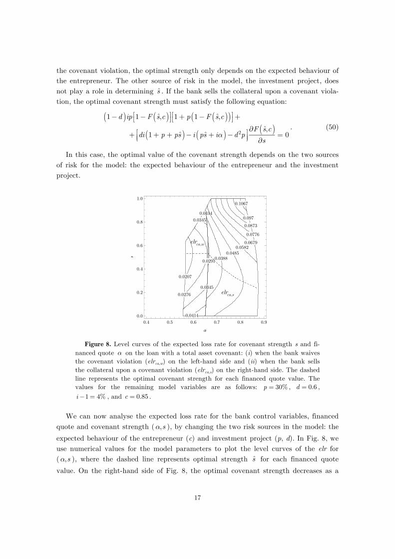
Figure 8. Level curves of the expected loss rate for covenant strength s and fi-

nanced quote α on the loan with a total asset covenant: (i) when the bank waives the covenant violation (elrca,w) on the left-hand side and (ii) when the bank sells the collateral upon a covenant violation (elrca,s) on the right-hand side. The dashed line represents the optimal covenant strength for each financed quote value. The values for the remaining model variables are as follows: p = 30% , d = 0.6 ,

i−1 = 4% , and c = 0.85 . We can now analyse the expected loss rate for the bank control variables, financed

quote and covenant strength ( α,s ), by changing the two risk sources in the model: the

expected behaviour of the entrepreneur (c) and investment project (p, d). In Fig. 8, we use numerical values for the model parameters to plot the level curves of the elr for ( α,s ), where the dashed line represents optimal strength s for each financed quote

value. On the right-hand side of Fig. 8, the optimal covenant strength decreases as a

18

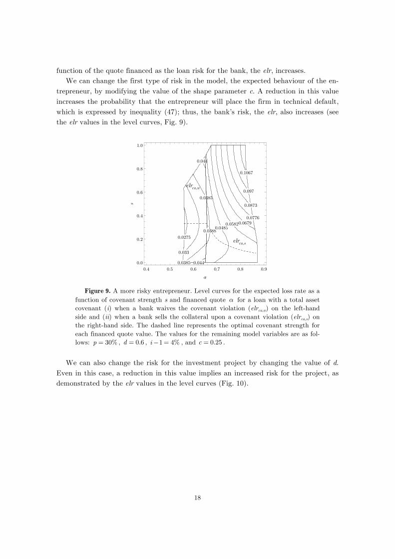
function of the quote financed as the loan risk for the bank, the elr, increases. We can change the first type of risk in the model, the expected behaviour of the en-

trepreneur, by modifying the value of the shape parameter c. A reduction in this value increases the probability that the entrepreneur will place the firm in technical default, which is expressed by inequality (47); thus, the bank’s risk, the elr, also increases (see the elr values in the level curves, Fig. 9).

0.0275

0.033

0.0385

0.0385

0.044

0.044

0.03880.0485

0.05820.06790.0776

0.0873

0.097

0.1067

0.4 0.5 0.6 0.7 0.8 0.90.0

0.2

0.4

0.6

0.8

1.0

a

s

elrca,s

elrca,w

Figure 9. A more risky entrepreneur. Level curves for the expected loss rate as a

function of covenant strength s and financed quote α for a loan with a total asset covenant (i) when a bank waives the covenant violation (elrca,w) on the left-hand side and (ii) when a bank sells the collateral upon a covenant violation (elrca,s) on the right-hand side. The dashed line represents the optimal covenant strength for each financed quote value. The values for the remaining model variables are as fol-lows: p = 30% , d = 0.6 , i−1 = 4% , and c = 0.25 .

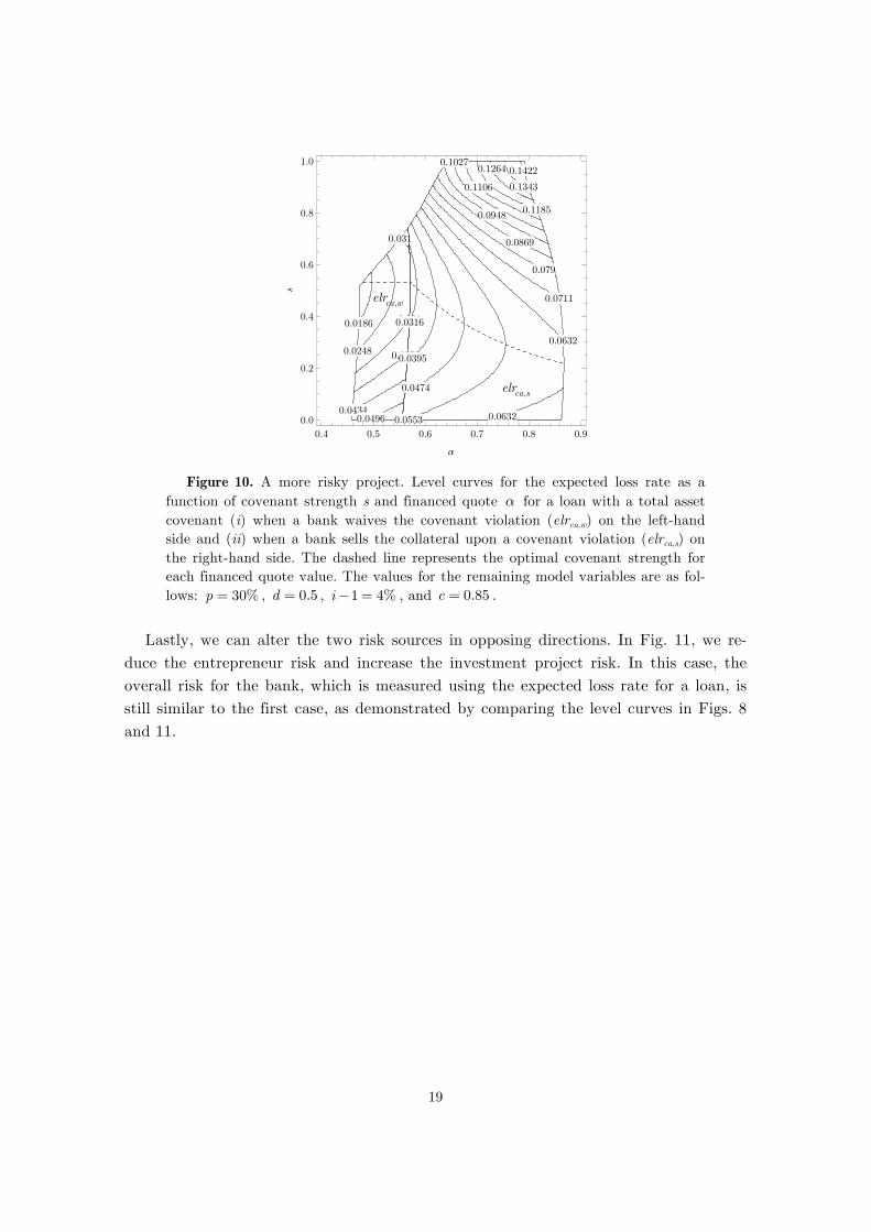
We can also change the risk for the investment project by changing the value of d.

Even in this case, a reduction in this value implies an increased risk for the project, as demonstrated by the elr values in the level curves (Fig. 10).

19

0.0186

0.0248

0.031

0.031

0.0372

0.04340.0496

0.0316

0.0395

0.0474

0.0553 0.0632

0.0632

0.0711

0.079

0.0869

0.0948

0.1027

0.1106

0.1185

0.1264

0.1343

0.1422

0.4 0.5 0.6 0.7 0.8 0.90.0

0.2

0.4

0.6

0.8

1.0

a

s

elrca,s

elrca,w

Figure 10. A more risky project. Level curves for the expected loss rate as a

function of covenant strength s and financed quote α for a loan with a total asset covenant (i) when a bank waives the covenant violation (elrca,w) on the left-hand side and (ii) when a bank sells the collateral upon a covenant violation (elrca,s) on the right-hand side. The dashed line represents the optimal covenant strength for each financed quote value. The values for the remaining model variables are as fol-lows: p = 30% , d = 0.5 , i−1 = 4% , and c = 0.85 .

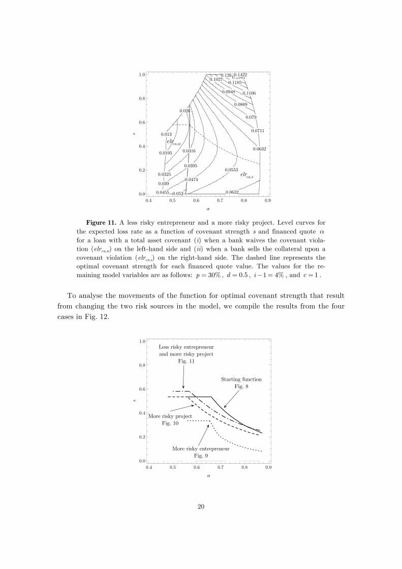
Lastly, we can alter the two risk sources in opposing directions. In Fig. 11, we re-

duce the entrepreneur risk and increase the investment project risk. In this case, the overall risk for the bank, which is measured using the expected loss rate for a loan, is still similar to the first case, as demonstrated by comparing the level curves in Figs. 8 and 11.

20

0.013

0.0195

0.026

0.0325

0.039

0.0455 0.052

0.0316

0.0395

0.0474

0.0553

0.0632

0.0632

0.0711

0.079

0.0869

0.0948

0.1027

0.1106

0.1185

0.12640.13430.1422

0.4 0.5 0.6 0.7 0.8 0.90.0

0.2

0.4

0.6

0.8

1.0

a

s

elrca,w

elrca,s

Figure 11. A less risky entrepreneur and a more risky project. Level curves for

the expected loss rate as a function of covenant strength s and financed quote α for a loan with a total asset covenant (i) when a bank waives the covenant viola-tion (elrca,w) on the left-hand side and (ii) when a bank sells the collateral upon a covenant violation (elrca,s) on the right-hand side. The dashed line represents the optimal covenant strength for each financed quote value. The values for the re-maining model variables are as follows: p = 30% , d = 0.5 , i−1 = 4% , and c = 1 .

To analyse the movements of the function for optimal covenant strength that result

from changing the two risk sources in the model, we compile the results from the four cases in Fig. 12.

0.0186

0.0248

0.031

0.031

0.0372

0.04340.0496

0.0316

0.0395

0.0474

0.0553 0.0632

0.0632

0.0711

0.079

0.0869

0.0948

0.1027

0.1106

0.1185

0.1264

0.1343

0.1422

0.4 0.5 0.6 0.7 0.8 0.90.0

0.2

0.4

0.6

0.8

1.0

a

s

Starting functionFig. 8

More risky projectFig. 10

More risky entrepreneurFig. 9

Less risky entrepreneurand more risky project

Fig. 11

21

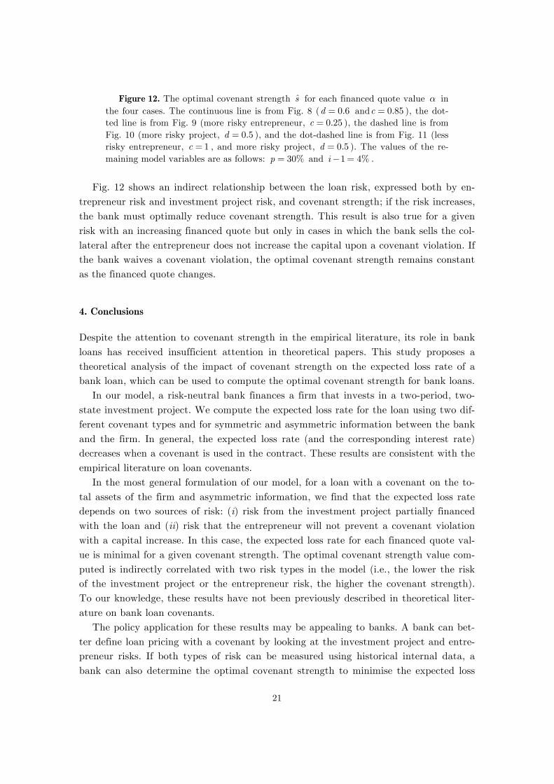
Figure 12. The optimal covenant strength s for each financed quote value α in the four cases. The continuous line is from Fig. 8 ( d = 0.6 and c = 0.85 ), the dot-ted line is from Fig. 9 (more risky entrepreneur, c = 0.25 ), the dashed line is from Fig. 10 (more risky project, d = 0.5 ), and the dot-dashed line is from Fig. 11 (less risky entrepreneur, c = 1 , and more risky project, d = 0.5 ). The values of the re-maining model variables are as follows: p = 30% and i−1 = 4% .

Fig. 12 shows an indirect relationship between the loan risk, expressed both by en-

trepreneur risk and investment project risk, and covenant strength; if the risk increases, the bank must optimally reduce covenant strength. This result is also true for a given risk with an increasing financed quote but only in cases in which the bank sells the col-lateral after the entrepreneur does not increase the capital upon a covenant violation. If the bank waives a covenant violation, the optimal covenant strength remains constant as the financed quote changes.

4. Conclusions

Despite the attention to covenant strength in the empirical literature, its role in bank loans has received insufficient attention in theoretical papers. This study proposes a theoretical analysis of the impact of covenant strength on the expected loss rate of a bank loan, which can be used to compute the optimal covenant strength for bank loans.

In our model, a risk-neutral bank finances a firm that invests in a two-period, two-state investment project. We compute the expected loss rate for the loan using two dif-ferent covenant types and for symmetric and asymmetric information between the bank and the firm. In general, the expected loss rate (and the corresponding interest rate) decreases when a covenant is used in the contract. These results are consistent with the empirical literature on loan covenants.

In the most general formulation of our model, for a loan with a covenant on the to-tal assets of the firm and asymmetric information, we find that the expected loss rate depends on two sources of risk: (i) risk from the investment project partially financed with the loan and (ii) risk that the entrepreneur will not prevent a covenant violation with a capital increase. In this case, the expected loss rate for each financed quote val-ue is minimal for a given covenant strength. The optimal covenant strength value com-puted is indirectly correlated with two risk types in the model (i.e., the lower the risk of the investment project or the entrepreneur risk, the higher the covenant strength). To our knowledge, these results have not been previously described in theoretical liter-ature on bank loan covenants.

The policy application for these results may be appealing to banks. A bank can bet-ter define loan pricing with a covenant by looking at the investment project and entre-preneur risks. If both types of risk can be measured using historical internal data, a bank can also determine the optimal covenant strength to minimise the expected loss

22

rate.

5. Acknowledgements

We would like to thank four anonymous referees, Franck Moraux, and the seminar par-ticipants at the AFFI 2008 Conference in Montpellier for providing comments that were helpful in developing this study. The usual disclaimer applies.

6. References

Basel Committee on Banking Supervision (2005), International Convergence of Capital Measurement and Capital Standards. A Revised Framework, BIS, Basel.

Duffie D., Singleton K.J. (2003), Credit Risk. Pricing, Measurement, and Management, Princeton University Press, Princeton.

Gupton G.M., Finger C.C., Bhatia M. (1997), CreditMetrics Technical Document, Risk Metrics Group, New York.

Lando D. (2004), Credit Risk Modeling. Theory and Applications, Princeton University Press, Princeton.

May W., Verde M. (2006), Loan Volumes Surge, Covenants Shrink in 2005, FitchRat-ings, New York.

Padgett C. (2006), Request for Comment on Moody’s Indenture Covenant Research & Assessment Framework, Moody’s Investors Service, New York.

Smith C., Warner J. (1979), On Financial Contracting: An Analysis of Bond Cove-nants, Journal of Financial Economics, 7 (June), pp. 117-61.

Standard & Poor’s (2006), Corporate Ratings Criteria, Standard & Poor’s, New York. Ackert, L.F., Huang, R., Ramirez, G.G., 2007. Information Opacity, Credit Risk, and

the Design of Loan Contracts for Private Firms. Financial Markets, Institutions & Instruments 16, 221–242.

Asquith, P., Beatty, A., Weber, J., 2005. Performance pricing in bank debt contracts. Journal of Accounting and Economics 40, 101–128.

Bazzana, F., Broccardo, E., 2012. The Role of Covenants in Public and Private Debt. mimeo.

Billett, M.T., Dolly King, T., Mauer, D., 2007. Growth Opportunities and the Choice of Leverage, Debt Maturity, and Covenants. The Journal of Finance 62, 697–730.

Black, F., Cox, J., 1976. Valuing Corporate Securities: Some Effects of Bond Indenture Provisions. The Journal of Finance 31, 351–367.

Demiroglu, C., James, C., 2010. The information content of bank loan covenants. The Review of Financial Studies 23, 3700–3737.

23

Garleanu, N., Zwiebel, J., 2009. Design and Renegotiation of Debt Covenants. The Re-view of Financial Studies 22, 749–781.

Godlewski, C.J., Weill, L., 2011. Does Collateral Help Mitigate Adverse Selection? A Cross-Country Analysis. Journal of Financial Services Research 40, 49–78.

Kwan, S.H., Carleton, W.T., 2010. Financial Contracting and the Choice between Pri-vate Placement and Publicly Offered Bonds. Journal of Money, Credit and Ban-king 42, 907–929.

Moir, L., Sudarsanam, S., 2007. Determinants of Financial Covenants and Pricing of Debt in Private Debt Contracts: The UK evidence. Accounting and Business Re-search 37, 151–166.

Nini, G., Smith, D.C., Sufi, A., 2009. Creditor control rights and firm investment poli-cy☆. Journal of Financial Economics 92, 400–420.

Niskanen, J., Niskanen, M., 2004. Covenants and Small Business Lending: The Finnish Case. Small Business Economics 23, 137–149.

Paglia, J., Mullineaux, D.J., 2006. An empirical exploration of financial covenants in large bank loans. Banks and Bank Systems 1, 103–122.

Rajan, R.G., Winton, A., 1995. Covenants and Collateral as Incentives to Monitor. The Journal of Finance 50, 1113–1146.

Sufi, A., 2009. Bank Lines of Credit in Corporate Finance: An Empirical Analysis. The Review of Financial Studies 22, 1057–1088.