SQUID microscopy

Milan Tomazin Adviser: prof. dr. Zvonko Trontelj

7th September 2003

Contents

1 Introduction 1

2 SQUID 2

3 Microscope 43.1 Apparatus . . . . . . . . . . . . . . . . . . . . . . . . . . . . . . . . . . . . . . 43.2 Properties . . . . . . . . . . . . . . . . . . . . . . . . . . . . . . . . . . . . . . 53.3 Measurements . . . . . . . . . . . . . . . . . . . . . . . . . . . . . . . . . . . . 73.4 Sensitivity . . . . . . . . . . . . . . . . . . . . . . . . . . . . . . . . . . . . . . 73.5 Applications . . . . . . . . . . . . . . . . . . . . . . . . . . . . . . . . . . . . . 9

4 Conclusion 11

1 Introduction

In this brief text, first the SQUID (Superconducting Quantum Interference Device), which isthe main part of the scanning SQUID microscope (SSM) is described. SSM is an extremelysensitive instrument for imaging local magnetic fields. The design and operation of the SSMare described, and several illustrations of the capabilities of this technique are presented. Theabsolute calibration of this instrument with an ideal point source, a single vortex trapped ina superconducting film, is shown.

1

2 SQUID

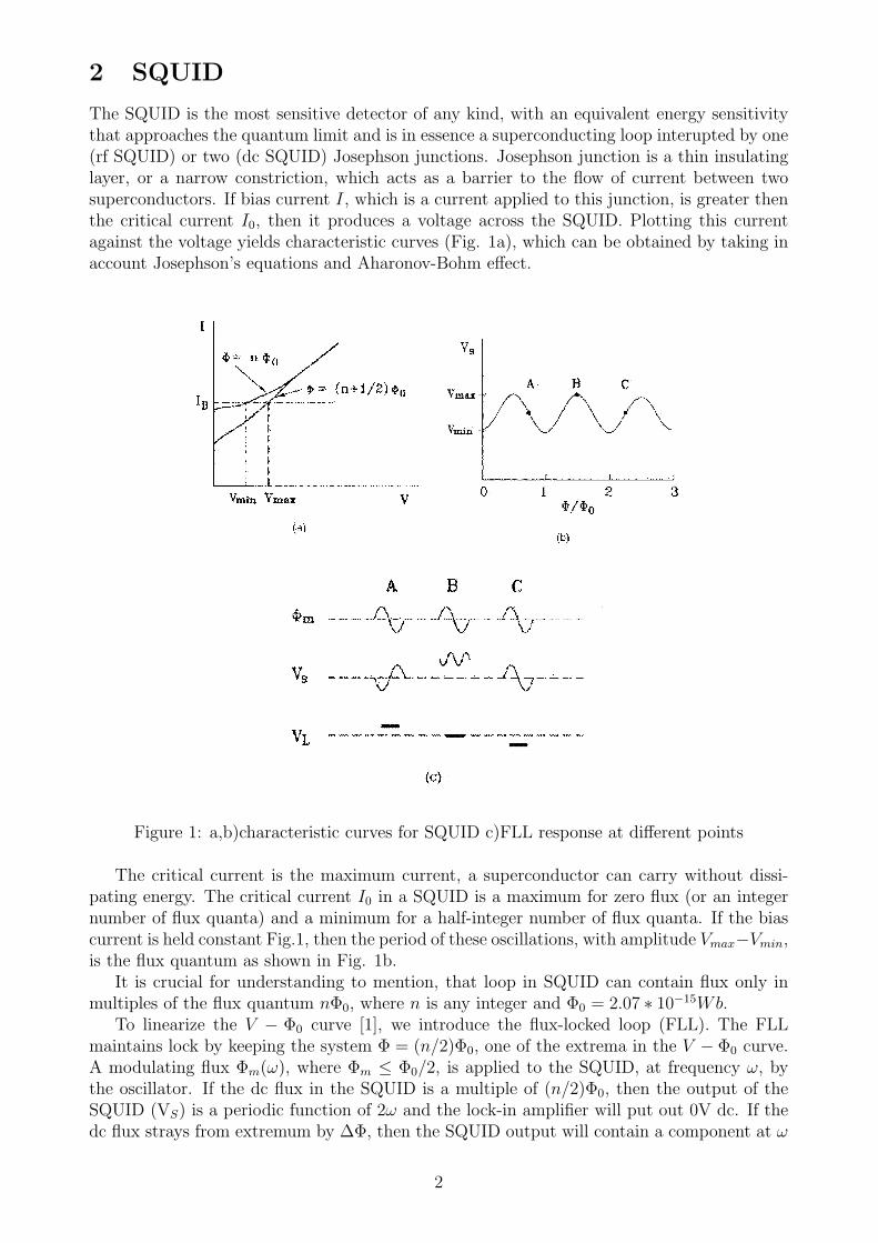
The SQUID is the most sensitive detector of any kind, with an equivalent energy sensitivitythat approaches the quantum limit and is in essence a superconducting loop interupted by one(rf SQUID) or two (dc SQUID) Josephson junctions. Josephson junction is a thin insulatinglayer, or a narrow constriction, which acts as a barrier to the flow of current between twosuperconductors. If bias current I, which is a current applied to this junction, is greater thenthe critical current I0, then it produces a voltage across the SQUID. Plotting this currentagainst the voltage yields characteristic curves (Fig. 1a), which can be obtained by taking inaccount Josephson’s equations and Aharonov-Bohm effect.

Figure 1: a,b)characteristic curves for SQUID c)FLL response at different points

The critical current is the maximum current, a superconductor can carry without dissi-pating energy. The critical current I0 in a SQUID is a maximum for zero flux (or an integernumber of flux quanta) and a minimum for a half-integer number of flux quanta. If the biascurrent is held constant Fig.1, then the period of these oscillations, with amplitude Vmax−Vmin,is the flux quantum as shown in Fig. 1b.

It is crucial for understanding to mention, that loop in SQUID can contain flux only inmultiples of the flux quantum nΦ0, where n is any integer and Φ0 = 2.07 ∗ 10−15Wb.

To linearize the V − Φ0 curve [1], we introduce the flux-locked loop (FLL). The FLLmaintains lock by keeping the system Φ = (n/2)Φ0, one of the extrema in the V − Φ0 curve.A modulating flux Φm(ω), where Φm ≤ Φ0/2, is applied to the SQUID, at frequency ω, bythe oscillator. If the dc flux in the SQUID is a multiple of (n/2)Φ0, then the output of theSQUID (VS) is a periodic function of 2ω and the lock-in amplifier will put out 0V dc. If thedc flux strays from extremum by ∆Φ, then the SQUID output will contain a component at ω

2

and the lock-in will put out a dc voltage (VL), proportional to the amplitude of the signal atω, as shown in Fig. 1c.

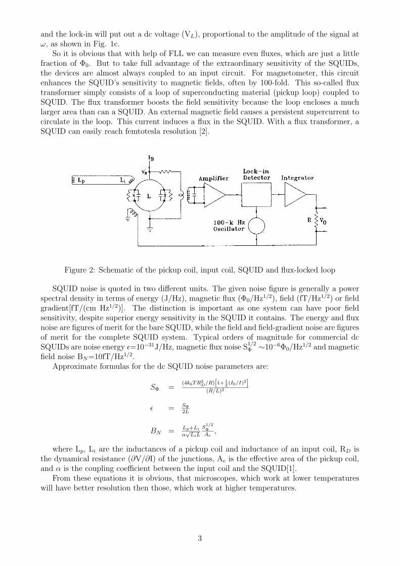
So it is obvious that with help of FLL we can measure even fluxes, which are just a littlefraction of Φ0. But to take full advantage of the extraordinary sensitivity of the SQUIDs,the devices are almost always coupled to an input circuit. For magnetometer, this circuitenhances the SQUID’s sensitivity to magnetic fields, often by 100-fold. This so-called fluxtransformer simply consists of a loop of superconducting material (pickup loop) coupled toSQUID. The flux transformer boosts the field sensitivity because the loop encloses a muchlarger area than can a SQUID. An external magnetic field causes a persistent supercurrent tocirculate in the loop. This current induces a flux in the SQUID. With a flux transformer, aSQUID can easily reach femtotesla resolution [2].

Figure 2: Schematic of the pickup coil, input coil, SQUID and flux-locked loop

SQUID noise is quoted in two different units. The given noise figure is generally a powerspectral density in terms of energy (J/Hz), magnetic flux (Φ0/Hz1/2), field (fT/Hz1/2) or fieldgradient[fT/(cm Hz1/2)]. The distinction is important as one system can have poor fieldsensitivity, despite superior energy sensitivity in the SQUID it contains. The energy and fluxnoise are figures of merit for the bare SQUID, while the field and field-gradient noise are figuresof merit for the complete SQUID system. Typical orders of magnitude for commercial dcSQUIDs are noise energy ε=10−31J/Hz, magnetic flux noise S

1/2Φ ∼10−6Φ0/Hz1/2 and magnetic

field noise BN=10fT/Hz1/2.Approximate formulas for the dc SQUID noise parameters are:

SΦ =(4kbTR2

D/R)[1+ 12(I0/I)2]

(R/L)2

ε = SΦ

2L

BN = Lp+Li

α√

LiL

S1/2Φ

Ae,

where Lp, Li are the inductances of a pickup coil and inductance of an input coil, RD isthe dynamical resistance (∂V/∂I) of the junctions, Ae is the effective area of the pickup coil,and α is the coupling coefficient between the input coil and the SQUID[1].

From these equations it is obvious, that microscopes, which work at lower temperatureswill have better resolution then those, which work at higher temperatures.

3

3 Microscope

Simply put, a SQUID microscope scans a sample relative to a SQUID to image the samplemagnetic fields. Immediately after the invention of the SUID magnetometer, the first device todo a two dimensional scan of a sample relative to a SQUID pickup loop was built. It happened1983 at IBM’s Watson Research center. With this device, it was able to detect individualvortices trapped in holes photolithographically patterned in thin films of niobium. The spatialresolution was determined by the size of the pickup loop, about 500 µm in diameter.

Figure 3: Both sample and sensor can be cooled (a-c) or only the SQUID (d-f). The fieldat the SQUID can be detected(a,d) or a superconducting loop can be inductively coupled tothe SQUID(b,e) or the pickup loop can be integrated into the SQUID design(c). In (f), aferromagnetic tip is used to couple flux from a room temperature sample to cooled SQUID.

Broadly speaking, these devices can be split into two classes [3], one with the sample at thetemperature of the SQUID (cold sample) and the other with the sample at room temperature(warm sample) as shown in Fig. 3. The main distinction is of course working temperature (atliquid helium or nitrogen) plus the warm sample microscope has a window, which is necessaryfor examination at room pressure.

3.1 Apparatus

Fig. 4 [4] shows a configuration of a high Tc microscope. As already mentioned is thisconfiguration very similar to the configuration of a low Tc microscope. The SQUID chip(b) is mounted in vacuum on top of a sapphire cold finger (e) that is clamped to a liquidnitrogen can (C). A thin vacuum window (a) is positioned above the SQUID chip by anadjusting mechanism (A) that allows the vacuum gap between the window and the SQUID tobe changed. A flux modulation coil (f) used to operate the SQUID in a FLL is wound on theend of the cold finger. The entire microscope is placed inside a triple-layered µ-metal can toattenuate the earth’s magnetic field and 60 Hz power line noise. For diminishing mechanicalnoise the whole device is suspended from the ceiling of a screened room with elastic cords.

The design of the vacuum window plays the key role in determing the minimum SQUID-sample separation at high Tc microscopes. This separation is given by the sum of the windowthickness, the window bow under atmospheric pressure, and the vacuum gap between thewindow and the SQUID. The sum decreases with increasing elastic modulus and decreasingwindow diameter. For this purpose is convenient to use material such as sapphire (E ∼345GPa) and silicon nitride SixNy (E ∼ 245GPa). The sum can be as low as few tens of µm.

4

Fig.4

3.2 Properties

A crucial parameter relevant to all SQUID microscopes is the separation z between the SQUIDand the sample. Under optimum circumstances the best spatial resolution that can be achievedfor the image of a magnetic object is approximately equal to z (Fig. 5), although the relativesizes of the object and the SQUID and the noise of the SQUID also play roles. Thus the greatadvantage of low Tc microscopes is that the SQUID can be brought into physical contactwith the sample, allowing one to achieve values of z as low as a few microns. Obviousdisadvantages of cold sample microscopes are that the sample size is constrained and that thetime required for thermally cycling is necessarily long. Furthermore, living samples that haveto be maintained at room temperature and pressure cannot be examined by Tc microscopesmade for operating at low temperatures.

The resolution of the instrument can be defined using a Rayleigh-like criterion, as illus-trated in Figure 4. This figure shows the cross sections predicted for the loop geometry andorientation of Figure 10 for two point vortices. The dashed lines are the individual contribu-tions, and the solid line is the total predicted signal. The spacing between the two vorticeshas been adjusted until the predicted minimum is 81% of the maxima. This happens fora spacing of 11.2 µm. The resolution of this tip-loop geometry and orientation is thereforedefine as 11.2 µm.

Figure 5 shows the predicted resolution and total flux coupling into the loop for magnetic”monopole” sources, such as superconducting vortices, using the Rayleigh-like criterion, as-suming a hexagonal pickup loop oriented parallel to the sample surface. This figure showsthat the ultimate resolution is set by the diameter of the loop, and that the signal falls offrapidly as the loop is moved away from the surface. These curves would look different, forexample, for a dipole source, but superconducting vortices provide a convenient calibrationpoint source for the scanning SQUID microscope.

5

Figure 4: Predicted SQUID output signal for two superconducting vortices separated by 11µm

Figure 5: Predicted resolution (upper curve) and maximum flux coupled (lower curve) for ahexagonal loop of diameter d, as a function of the height z above the sample plane, using aRayleigh-like criterion

6

3.3 Measurements

The SQUID sensor requires a cryogenic environment, since it must be superconducting tooperate. The desired scan area, at least a few hundred microns on a side, is extremely diffi-cult to attain at low temperatures using piezoelectric scanning elements. To obtain optimalresolution, it is necessary to make the pickup loop of the SQUID very small, well shielded,and positioned as close as possible to the sample surface.

3.4 Sensitivity

Figure 6 illustrates the sensitivity of the scanning SQUID microscope to permanent magneticmoments. This image is of the magnetic field about 15 µm above the surface of a floppy disk.This particular image was taken with the pickup loop plane oriented normal to the sampleand nearly parallel to the track axis (nearly horizontal in this image). The region of the floppydisk that is being imaged contains alignment marks with magnetic domains with moments inthe plane of the surface, oriented in alternate directions normal to the track direction. Thefalse-colour coding of this image, uses a spectral distribution from dark blue to bright red. Inthis image dark blue represents flux passing through the loop in one direction, while red isflux in the opposite direction. The total scale represented by the false-colour imaging schemeis about 30Φ0 change in flux through the SQUID pickup loop, corresponding to a total fieldvariation of about 5 gauss. Since the effective noise of the SQUID and electronics, expressedas an effective noise at the SQUID loop, is typically about 2·10−6Φ0, and images are takenat a pixel rate of about 5 Hz, this means that such an image has a potential signal-to-noiseratio of order 10−7. Other factors, such as the dynamic range of amplifiers and analog-digitalconverters, limit the actual signal-to-noise ratio, and there are easier methods for imaging bitpatterns, but this is clearly a very sensitive technique.

Figure 6: Magnetic image of the alignment track on floppy disk. The false-colour lookup tablescans a range of 30 flux quanta treading the 10 µm diameter pickup loop, oriented normal tothe disk surface, with its plane parallel to the bottom of the image.

Figure 7 illustrates the sensitivity of the scanning SQUID microscope to externally appliedfields. This is an image of the magnetic field about 2.5 µm above a thin-film superconductingniobium meander with 10 µm linewidth and spacing. This image was taken with the 10 µmdiameter pickup loop oriented about 20o from parallel to the sample. An external magneticfield of about 5.4 mG was applied to the sample to make the superconducting meander visible.Meissner exclusion of magnetic field from the sample screens the sensor from the applied fieldabove the meander, and concentrates the field in the interline regions. Meissner screening bysuperconducting thin films is very useful for making index marks for the scanning SQUID

7

microscope using superconducting thin films. The index marks can be made visible by apply-ing a small external field, and made nearly invisible by turning the field off. The ”ghosting”visible in the bottom of this image is caused by additional pickup from the unshielded pickupleads.

Figure 7: Magnetic image of the normal component of the field above a superconductingniobium thin-film meander, in the presence of an externally applied 5.3 mG field.

Figure 8 illustrates the sensitivity of the scanning SQUID microscope to electrical currents.This image is of the upper third of the same niobium thin-film meander as in Figure 7. In thiscase the 10 µm diameter SQUID pickup loop is oriented perpendicular to the sample plane,and nearly parallel to the long lines in the meander pattern. A 134 Hz, 100 nA ac currentis applied to the meander. The signal from the SQUID is phase sensitively detected usinga lock-in amplifier. The image shows alternating magnetic field directions associated withthe alternating current directions as the current follows the meander pattern. The effectivenoise at the SQUID loop is 2.5·10−6Φ0, corresponding to an effective current noise of about 1nA/

√Hz.

Figure 8: Magnetic image of the field component parallel to the bottom of the image, due to100nA ac current through the superconducting niobium meander imaged in Figure 7. Thisimage includes just the top third of the meander.

8

3.5 Applications

Imaging of superconducting circuitry

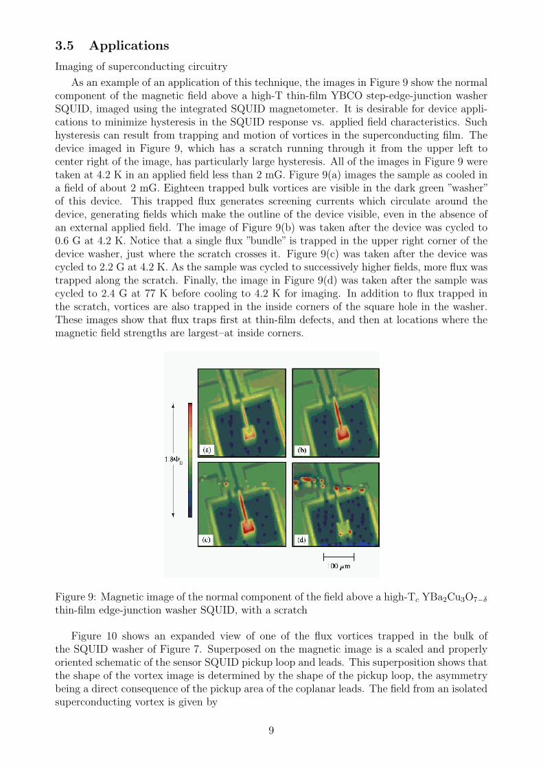
As an example of an application of this technique, the images in Figure 9 show the normalcomponent of the magnetic field above a high-T thin-film YBCO step-edge-junction washerSQUID, imaged using the integrated SQUID magnetometer. It is desirable for device appli-cations to minimize hysteresis in the SQUID response vs. applied field characteristics. Suchhysteresis can result from trapping and motion of vortices in the superconducting film. Thedevice imaged in Figure 9, which has a scratch running through it from the upper left tocenter right of the image, has particularly large hysteresis. All of the images in Figure 9 weretaken at 4.2 K in an applied field less than 2 mG. Figure 9(a) images the sample as cooled ina field of about 2 mG. Eighteen trapped bulk vortices are visible in the dark green ”washer”of this device. This trapped flux generates screening currents which circulate around thedevice, generating fields which make the outline of the device visible, even in the absence ofan external applied field. The image of Figure 9(b) was taken after the device was cycled to0.6 G at 4.2 K. Notice that a single flux ”bundle” is trapped in the upper right corner of thedevice washer, just where the scratch crosses it. Figure 9(c) was taken after the device wascycled to 2.2 G at 4.2 K. As the sample was cycled to successively higher fields, more flux wastrapped along the scratch. Finally, the image in Figure 9(d) was taken after the sample wascycled to 2.4 G at 77 K before cooling to 4.2 K for imaging. In addition to flux trapped inthe scratch, vortices are also trapped in the inside corners of the square hole in the washer.These images show that flux traps first at thin-film defects, and then at locations where themagnetic field strengths are largest–at inside corners.

Figure 9: Magnetic image of the normal component of the field above a high-Tc YBa2Cu3O7−δ

thin-film edge-junction washer SQUID, with a scratch

Figure 10 shows an expanded view of one of the flux vortices trapped in the bulk ofthe SQUID washer of Figure 7. Superposed on the magnetic image is a scaled and properlyoriented schematic of the sensor SQUID pickup loop and leads. This superposition shows thatthe shape of the vortex image is determined by the shape of the pickup loop, the asymmetrybeing a direct consequence of the pickup area of the coplanar leads. The field from an isolatedsuperconducting vortex is given by

9

~B(~r) =Φ0

2πr3~r

for distances r much greater than the penetration depth. The sensitivity of this instrumentcan be estimated by considering a circular loop of radius r parallel to a superconducting surfaceand centered a height h above a flux vortex trapped in the superconductor. The total fluxthrough this loop is

Φloop = Φ0[1−h/r√

(h/r)2 + 1]

At the easily attained height h = r, the amount of flux coupling into the pickup loopis about 0.3. This image is taken at about 5 pixels/s, which means that with a SQUIDnoise of 2·10−6

√Hz an individual vortex can be imaged with an electronic signal-to-noise

ratio of about 7·104. Actual signal-to-noise ratios, although limited by scanning irregularitiesapparently arising from tip-sample interactions, are nevertheless remarkably good, as can beseen from the cross sections in Figure 10. The solid lines in Figure 10 are fits to the datanumerically integrating equation (3.5), using the known pickup loop and lead geometry, theknown angle of the SQUID plane relative to the sample plane, with the distance betweenthe tip and the pickup loop center as the only fitting parameter. The best fit was obtainedfor a distance of 8 µm, in reasonable agreement with microscopic inspection of the tip afterpolishing. The fits show that we there is a good understanding of the absolute magnitudeand general shape of the observed vortex images.

Figure 10: Expanded view of Fig. 9 scanned in two different paths. The right graph presentsnumericaly fitting data.

10

4 Conclusion

In conclusion, the scanning SQUID microscope represents a very sensitive instrument forimaging local magnetic fields. It can be achieved something better resolution then 10µm.Ultimately an order of magnitude better resolution should be possible. The sensitivity ofthis instrument is such that spins of about a hundred µB , or currents of a few nA, can beimaged. This sensitivity allows measurements that would be extremely difficult using anyother technique.

Figure 11: Sensitivity of different types of magnetic probes

References

[1] William G. Jenks, SQUIDS: Encyclopedia of Applied Physics, Vol.19 (1997), 457-468

[2] John Clarke, SQUIDs: Scientific American, August 1994

[3] J.R.Kirtley, SQUID microscopy for fundamental studies, Physica C 368(2002) 55-65

[4] Thomas S. Lee, Yann R. Chemla, Eugene Dantsker, John Clarke, High-Tc SQUID Micro-scope for Room Temperature Samples, IEEE Transactions on applied superconductivity,vol. 7, no. 2, june 1997

11